andrea goldsmith and ivana maric´ - stanford...
TRANSCRIPT

Chapter 2
Capacity of Cognitive Radio Networks
Andrea Goldsmith and Ivana Maric

2.1. INTRODUCTION 1
2.1 Introduction
This chapter develops the fundamental capacity limits and associated transmission
techniques for different cognitive radio network paradigms. These limits are based on
the premise that the cognitive radios of secondary users are intelligent wireless com-
munication devices that exploit side information about their environment to improve
spectrum utilization. This side information typically comprises knowledge about the
activity, channels, encoding strategies and/or transmitted data sequences of the primary
users with which the secondary users share the spectrum. Based on the nature of the
available side information as well as a priori rules about spectrum usage, cognitive ra-
dio systems seek to underlay, overlay or interweave the secondary users’ signals with
the transmissions of primary users. This chapter develops the fundamental capacity
limits for all three cognitive radio paradigms. These capacity limits provide guidelines
for the spectral efficiency possible in cognitive radio networks, as well as practical
design ideas to optimize performance of such networks.
While the general definition of cognitive radio was provided in Chapter 1, we now
interpret that definition in a mathematically precise manner that can be used in the
development of cognitive radio capacity limits. Specifically, in the mathematical ter-
minology of information theory, it is the availability and utilization of network side
information that defines a cognitive radio, which we formalize as follows:
A cognitive radio is a wireless communication device that intelligently utilizes any
available side information about the (a) activity, (b) channel conditions, (c) encoding
strategies or (d) transmitted data sequences of primary users with which it shares the
spectrum.
Based on the type of available network side information along with the regulatory
constraints, secondary users seek to underlay, overlay, or interweave their signals with
those of primary users without significantly impacting these users [51]. In the next
section we describe these different cognitive radio paradigms in more detail. The fun-
damental capacity limits for each of these paradigms are discussed in later sections.
2.2 Cognitive Radio Network Paradigms
There are three main cognitive radio network paradigms: underlay, overlay, and inter-
weave. The underlay paradigm allows secondary users to operate if the interference
they cause to primary users is below a given threshold or meets a given bound on pri-
mary user performance degradation. In overlay systems the secondary users overhear
the transmissions of the primary users, then use this information along with sophisti-
cated signal processing and coding techniques to maintain or improve the performance
of primary users, while also obtaining some additional bandwidth for their own com-
munication. Under ideal conditions, sophisticated encoding and decoding strategies
allow both the secondary and primary users to remove all or part of the interference
caused by other users. In interweave systems the secondary users detect the absence of
primary user signals in space, time, or frequency, and opportunistically communicate
during these absences. For all three paradigms, if there are multiple secondary users
then these users must share bandwidth amongst themselves as well as with the primary

2
users, subject to their given cognitive paradigm. This gives rise to the medium access
control (MAC) problem among secondary users similar to that which arises among
users in conventional wireless networks. Given this similarity, MAC protocols that
have been proposed for secondary users within a particular paradigm are often derived
from conventional MAC protocols. In addition, multiple secondary users may transmit
to a single secondary receiver, as in the uplink of a cellular or satellite system, and
one secondary user may transmit to multiple secondary receivers, as in the correspond-
ing downlink. We now describe each of the three cognitive radio paradigms in more
detail, including the associated regulatory policy as well as underlying assumptions
about what network side information is available, how it is used, and the practicality of
obtaining this information.
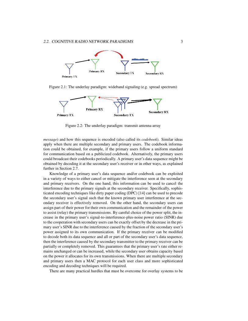
2.2.1 Underlay Paradigm
The underlay paradigm, shown in Figures 2.1 and 2.2, mandates that concurrent pri-
mary and secondary transmissions may occur only if the interference generated by the
secondary transmitters at the primary receivers is below some acceptable threshold.
Rather than determining the exact interference it causes, a secondary user can spread
its signal over a very wide bandwidth such that the interference power spectral density
is below the noise floor at any primary user location. These spread signals are then
despread at each of their intended secondary receivers. This spreading technique is the
basis of both spread spectrum and ultrawideband (UWB) communications [88]. Al-
ternatively, the secondary transmitter can be very conservative in its output power to
ensure that its signal remains below the prescribed interference threshold. In this case,
since the interference constraints in underlay systems are typically quite restrictive, this
limits the secondary users to short range communications. Both spreading and severe
restriction of transmit power avoid exact calculation of secondary user interference at
primary receivers, instead using a conservative design whereby the collective interfer-
ence of all secondary transmissions is small everywhere. This collective interference,
sometimes called the interference temperature [12], is discussed in more detail in Sec-
tion 4.2. Determining the exact interference a secondary transmitter causes to a primary
receiver is one of the biggest challenges in underlay systems. The secondary user can
determine this interference at a given primary receiver by overhearing a transmission
from that primary user if the link between them is reciprocal. For MIMO systems,
a secondary user only interferes with a primary user in their overlapping spatial di-
mensions. If the secondary user occupies only the null space of the MIMO primary
receiver, no interference is caused, and hence this falls within the interweave paradigm
discussed below, whereby the primary and secondary users occupy orthogonal spatial
dimensions. The underlay paradigm is most common in the licensed spectrum, where
the primary users are the licensees, but it can also be used in unlicensed bands to pro-
vide different classes of service to different users.
2.2.2 Overlay Paradigm
The premise for overlay systems, illustrated in Fig. 2.3, is that the secondary trans-
mitter has knowledge of the primary user’s transmitted data sequence (also called its
2.2. COGNITIVE RADIO NETWORK PARADIGMS 3
Figure 2.1: The underlay paradigm: wideband signaling (e.g. spread spectrum)
Figure 2.2: The underlay paradigm: transmit antenna array
message) and how this sequence is encoded (also called its codebook). Similar ideas
apply when there are multiple secondary and primary users. The codebook informa-
tion could be obtained, for example, if the primary users follow a uniform standard
for communication based on a publicized codebook. Alternatively, the primary users
could broadcast their codebooks periodically. A primary user’s data sequence might be
obtained by decoding it at the secondary user’s receiver or in other ways, as explained
further in Section 2.7.
Knowledge of a primary user’s data sequence and/or codebook can be exploited
in a variety of ways to either cancel or mitigate the interference seen at the secondary
and primary receivers. On the one hand, this information can be used to cancel the
interference due to the primary signals at the secondary receiver. Specifically, sophis-
ticated encoding techniques like dirty paper coding (DPC) [14] can be used to precode
the secondary user’s signal such that the known primary user interference at the sec-
ondary receiver is effectively removed. On the other hand, the secondary users can
assign part of their power for their own communication and the remainder of the power
to assist (relay) the primary transmissions. By careful choice of the power split, the in-
crease in the primary user’s signal-to-interference-plus-noise power ratio (SINR) due
to the cooperation with secondary users can be exactly offset by the decrease in the pri-
mary user’s SINR due to the interference caused by the fraction of the secondary user’s
power assigned to its own communication. If the primary receiver can be modified
to decode both its data sequence and all or part of the secondary user’s data sequence,
then the interference caused by the secondary transmitter to the primary receiver can be
partially or completely removed. This guarantees that the primary user’s rate either re-
mains unchanged or can be increased, while the secondary user obtains capacity based
on the power it allocates for its own transmissions. When there are multiple secondary
and primary users then a MAC protocol for each user class and more sophisticated
encoding and decoding techniques will be required.
There are many practical hurdles that must be overcome for overlay systems to be

4
successful. These include the technical challenges of overhearing primary user trans-
missions and decoding them, as well as the encoding and decoding complexity associ-
ated with secondary users in these systems. Moreover, sharing of primary user private
data sequences with secondary users, even when encrypted, will raise significant se-
curity and privacy concerns for the primary system. These significant challenges may
preclude overlay implementations in some types of systems. However, many of these
challenges can be overcome in certain settings, especially when the primary user data
is not private, e.g. in a cellular overlay within the TV broadcast spectrum [72]. Note
that the overlay paradigm can be applied to either licensed or unlicensed band com-
munications. In licensed bands, secondary users would be allowed to share the band
with the licensed users since they would not interfere with, and might even improve,
their communication. In unlicensed bands secondary users would provide more effi-
cient spectral user by exploiting knowledge of the primary users’ data sequences and
encoding strategies to reduce interference.
Figure 2.3: The overlay paradigm
2.2.3 Interweave Paradigm
The interweave paradigm is based on the idea of opportunistic communication, and
was the original motivation for cognitive radio [62]. The idea came about after studies
conducted by the FCC [24], universities [6], and industry [80] showed that a major
part of the spectrum is not fully utilized most of the time. In other words, there exist
temporary space-time-frequency voids, referred to as spectrum holes or white spaces,
that are not in constant use in both the licensed and unlicensed bands, as shown in
Fig. 2.4. The spatial spectrum holes may be in a single spatial dimension or, for MIMO
devices, in the subset of spatial dimensions not occupied by the primary users (i.e. in
the null space of the primary users’ receivers) [101]. Spectral holes can be exploited
by secondary users to operate in orthogonal dimensions of space, time or frequency
relative to the primary user signals. Thus, the utilization of spectrum is improved
by opportunistic reuse over the spectrum holes. The interweave technique requires
detection of primary (licensed or unlicensed) users in one or more of the space-time-
frequency dimensions. This detection is quite challenging since primary user activity
changes over time and also depends on geographical location. Chapters 4 and 5 discuss
spectrum hole detection by a single receiver and by multiple receivers, respectively, in

2.2. COGNITIVE RADIO NETWORK PARADIGMS 5
more detail. Interweave systems can also be applied to networks where all users in
a given band have equal priority, but existing users are treated as primary users, and
new users become secondary users that cannot interfere with communications already
taking place between existing users.
For interweave networks with multiple secondary users, a MAC protocol is needed
to share the available spectrum holes amongst them. Given the similarity of this prob-
lem with medium access control in conventional networks, the protocols that have been
proposed for this setting are often derived from conventional MAC protocols such as
ALOHA and CSMA [13]. Simple time-sharing mechanisms may also be used, and this
can greatly simplify capacity analysis. Advanced MAC protocols for multiuser inter-
weave networks utilize additional spatial degrees of freedom from multiple antennas,
optimization based on more advanced mathematical models such as partially-observed
Markov chains, or game theory and pricing mechnanisms [101, 102, 89, 43]. The chal-
lenge to medium access in the interweave setting above and beyond what has been
addressed in conventional MAC protocols is that the channel to be shared is unknown,
since it depends on the activity of the primary users. This primary user activity will
depend on the MAC protocol of the primary system, which is designed completely
independently of the secondary system. Given the many variants of MAC protocols
for conventional systems, developing an effective MAC protocol for secondary users
remains one of the biggest challenges in interweave system design.
To summarize, an interweave cognitive radio is an intelligent wireless commu-
nication system that periodically monitors the radio spectrum, detects primary user
occupancy over time, space, and frequency, and opportunistically communicates over
spectrum holes with minimal interference to the primary users. Additional motivation
and discussion of the signal processing challenges faced in interweave cognitive radio
is discussed in [41], as well as in Chapters 4 and 5.
Figure 2.4: Spectral occupancy measurements up to 6 GHz in an urban area at mid-day
(Berkeley Wireless Research Center (BWRC) [6]).

6
2.2.4 Comparison of Cognitive Radio Paradigms
Underlay Overlay Interweave
Network Side Information:
Secondary transmitters know
interference caused to primary
receivers.
Network Side Information:
Secondary nodes know chan-
nel gains, encoding techniques
and possibly the transmitted
data sequences of the primary
users.
Network Side Information:
Secondary users identify
spectrum holes in space, time,
and/or frequency from which
the primary users are absent.
Simultaneous Transmission:
Secondary users can trans-
mit simultaneously with the
primary users as long as
interference caused is below
an acceptable limit.
Simultaneous Transmission:
Secondary users can transmit
simultaneously with the pri-
mary users; the interference
to the primary users can be
offset by using part of the
secondary users’ power to
relay the primary users’ data
sequences.
Simultaneous Transmission:
Secondary users transmit
simultaneously with a primary
user only when there is missed
detection of the primary user
activity.
Transmit Power Limits: Sec-
ondary user’s transmit power
is limited by a constraint on
the interference caused to the
primary users.
Transmit Power Limits: Sec-
ondary users can transmit at
any power, the interference to
primary users can be offset
by relaying the primary users’
data sequences.
Transmit Power Limits: Sec-
ondary user’s transmit power
is limited by the range of
primary user activity it can de-
tect (alone or via cooperative
sensing).
Hardware: Secondary users
must measure the interference
they cause to primary users’
receivers by either sounding
and exploiting channel reci-
procity or via cooperative
sensing.
Hardware: Secondary users
must also listen to primary user
transmissions. Encoding and
decoding complexity is also
significantly higher than other
paradigms.
Hardware: Receiver must be
frequency agile or have a wide-
band front end for spectrum
hole detection.
Table 2.1: Comparison of underlay, overlay and interweave cognitive radio techniques.
Table 2.1 summarizes the differences among the underlay, overlay and interweave
cognitive radio approaches. While underlay and overlay techniques permit concurrent
primary and secondary user transmissions, avoiding simultaneous transmissions with
primary users in overlapping dimensions of time, space, or frequency is the main goal
in the interweave technique. We also point out that the cognitive radio approaches re-
quire different amounts of side information: underlay systems require knowledge of the
interference caused by the secondary transmitters to the primary receivers, interweave
systems require considerable side information about the primary user activity (which

2.3. FUNDAMENTAL PERFORMANCE LIMITS OF WIRELESS NETWORKS 7
can be obtained from sensing at one or more cognitive nodes in the system) and overlay
systems require a large amount of side information (knowledge of the primary user’s
encoding technique and possibly its transmitted data sequence, along with the channel
conditions in the network). Apart from device level power limits, the secondary user’s
transmit power in the underlay and interweave approaches is decided by the interfer-
ence constraint and range of sensing, respectively. Finally, hardware requirements vary
across the different paradigms, as discussed in more detail in Chapter 1.7. While un-
derlay, overlay and interweave are three distinct approaches to cognitive radio, hybrid
schemes can also be constructed that combine the advantages of different approaches.
For example, the overlay and interweave approaches are combined in [96].
2.3 Fundamental Performance Limits of Wireless Net-
works
A wireless network consists of a collection of wireless devices communicating over
a common wireless channel. The simplest wireless network consists of a single-user
(point-to-point) channel. In general, a wireless network contains multiple source nodes,
each communicating its information to a set of destination nodes. A wireless network
can have a supporting infrastructure (e.g. as in cellular networks), or an ad hoc struc-
ture, where nodes self-configure into a network and control is decentralized among the
nodes. The typical topologies of multiuser channels (in isolation or within one cell of a
cellular system) are multiple access (many transmitters to one receiver) and broadcast
(one transmitter to many receivers) channels. These channels correspond, respectively,
to the uplink and downlink of a satellite system or one base station in a cellular system.
In these networks, communication occurs between a group of nodes transmitting to or
receiving from a single node. In an ad hoc wireless network, each node can serve as a
source, destination and/or relay forwarding data for other users.
In cognitive radio applications, primary and secondary users accessing the same
spectrum form a wireless network. Primary and secondary users have different trans-
mit/receive constraints due to interference limitations at the primary receivers, as well
as possibly different transmit/receive capabilities. In cognitive radio networks the pri-
mary users can be cellular or ad hoc, whereas the secondary users are generally ad
hoc and fall into the paradigms of underlay, interweave or overlay. Hence, these two
types of cognitive radio network users form a two-tier wireless network. Performance
limits of wireless networks are thus of direct relevance to the performance limits of
cognitive radio networks. In particular, the fundamental capacity limits of ad hoc net-
works not only dictate how much information can be transmitted by secondary users
under a given set of network and interference conditions, but also limitations on the
information exchange possible between sensing nodes to collaboratively assess spec-
tral occupancy. In the following section we describe the broad range of performance
metrics relevant to wireless networks, including their capacity. We then formally de-
fine mutual information and capacity for single-user channels as well as for general
wireless networks.

8
2.3.1 Performance Metrics
The fundamental performance limits of a wireless network define their best possible
performance relative to one or more specific metrics. Many different metrics can be
used to measure performance, such as capacity, throughput, outage, energy consump-
tion, as well as combinations of these and other metrics. Since wireless networks ex-
hibit significant dynamics (user movement, data traffic, channel variations, etc.), these
dynamics must be taken into account in the definition of the network performance met-
rics.
The most common fundamental performance limit for time-invariant communica-
tion systems is Shannon capacity [78] - the maximum rate that can be achieved over
a channel with asymptotically small probability of error. Shannon’s simple yet ele-
gant mathematics coupled with his revolutionary ideas for coding over noisy channels
and bounding their fundamental data rate limits via mutual information has inspired
generations of theorists and practitioners, and provided significant insights into com-
munication system design. For single-user channels the Shannon capacity is a number,
the maximum data rate of the channel, as will be defined mathematically in terms of the
channel’s maximum mutual information in the next section. For a multiuser (broadcast
or multiple access) channel Shannon capacity is a K-dimensional region defining the
maximum rates possible for all K users simultaneously. Shannon capacity of wire-
less single-user and multiuser channels is known in many cases, including static and
time-varying single-user, broadcast and multiple access channels with noise, fading,
multipath, and/or multiple antennas [18, 4, 33].
Time-varying channels are typically modeled based on the notion of a channel
state. The channel state s lies within the set Sc of all possible channel states, which
may be discrete or continuous. For stationary and ergodic time-varying channels, at
any given time the channel is assumed to be in state s with probability p(s). This
model is also refered to as a composite channel [21]. The Shannon capacity or capacity
region of a time-varying stationary and ergodic channel is therefore called the ergodic
capacity, since it corresponds to the data rate or rate region in a particular channel
state (e.g. a particular fading value) averaged over the probability distribution of the
channel states (e.g. the fading distribution). An alternate performance metric for such
channels is outage capacity, whereby transmission to one or more users is suspended
in some channel states, deemed outage states, and a fixed transmission rate is used in
the nonoutage states. The outage capacity is then the maximum fixed rate that can be
achieved in nonoutage states with asymptotically small probability of error multiplied
by the probability of nonoutage. The outage capacity metric is based on the underly-
ing assumption that the transmitter knows the channel state and suspends transmission
during outage.
Another performance metric for time-varying channels when the channel state is
not known at the transmitter is capacity versus outage probability. In this case the
transmitter cannot adapt to channel conditions; it therefore selects a given rate C or set
of rates C to transmit to the user(s). If the channel supports these rates, i.e. the rates
are within the capacity of the channel under its realized channel state, then the data is
received without error; if not errors occur which are deemed a data outage. For single-
user channels the capacity versus outage probability metric takes the form of a plot

2.3. FUNDAMENTAL PERFORMANCE LIMITS OF WIRELESS NETWORKS 9
characterizing the capacity C associated with each outage probility Pout. This plot,
illustrated in Fig. 2.5a for a continuous-state single-user channel, thus corresponds to
the transmitter’s data rate versus the probability that this rate cannot be supported by
a given channel. The plot of C versus Pout is nondecreasing with Pout, since at high
outage probability more of the bad channel states need not support rate C , and hence
a higher capacity can be achieved in the nonoutage states. Consider now a finite-state
channel, where the set of channel states Sc is finite, and assume the states are ordered
so that the capacity Ci in state i satisfies Ci ≤ Cj for i ≤ j. Then C versus Pout has
a staircase shape with discrete increases for each n such that Pout =∑n
i=1 pi where
pi is the probability of the ith channel state. For example, in a two state channel with
capacity Ci for state i and state probability pi, i = 1, 2, if C1 < C2 then capacity
versus outage is C2 for Pout ≥ p1 and C1 for Pout < p1, as shown in Fig. 2.5b. More
details on ergodic capacity, outage capacity, and capacity versus outage can be found
in [32, 4, 33, 87]. Note that when the channel is nonergodic, such that the channel state
is chosen at random from the set Sc and remains constant for all time, the channel is
referred to as a compound channel. In this case the capacity generally corresponds to
achievable rates associated with the worst-case channel state [91].
Figure 2.5: Capacity versus outage probability for a single-user channel.
Capacity results are much more limited for general wireless networks with multiple
sources and multiple destinations, even for simple static models. For a K-node network
where each node is both a source and a destination, the capacity is a K × (K − 1)-dimensional region defining the maximum rates achievable between all node pairs.
Such regions are typically characterized by two-dimensional slices, which define the
maximum rates between two source-destination pairs in the network. More general
capacity regions whereby one source sends data to multiple destinations, also called
multicasting, can also be analyzed but we do not consider multicast in our network
models. In practice wireless networks often include multihop routing via relaying,
whereby intermediate nodes relay data toward its final destination. Such relaying can
increase the achievable data rates for the network as well as other performance met-
rics, often significantly [85]. Other advanced capabilities in the system design, such
as power control, multiple frequency bands to enable frequency reuse (the reuse of the
same frequency at spatially-separate locations), and interference cancellation can fur-
ther increase network performance. This is illustrated in Fig. 2.6 (from [85]), where a
two-dimensional capacity region slice for a five node network is illustrated for differ-

10
ent design assumptions about the network. We see from this figure that spatial reuse of
frequencies, multihop routing, and interference cancellation all significantly increase
the achievable rates within this slice.
Figure 2.6: Capacity region slice for node pairs (1,2) and (3,4) of a five-node wireless
network (a) Single-hop routing, no spatial reuse. (b) Multihop routing, no spatial reuse.
(c) Multihop routing with spatial reuse. (d) power control added to (c). (e) Successive
Interference Cancellation (SIC) added to (c).
The Shannon capacities for many of the most basic wireless networks, including the
three-node relay channel and the four-node interference channel, illustrated in Fig. 2.7,
have remained open problems for decades. This makes it unlikely that the capacity re-
gion can be obtained exactly for these and other similar networks, especially when the
number of users is larger than in these canonical examples. Instead, capacity regions
are often characterized by their upper and lower bounds rather than the exact region
(where these bounds meet). Lower bounds are easier to obtain than upper bounds,
as any communication scheme yields an achievable rate region that lower bounds the
capacity region. Upper bounds are more difficult to obtain as they must contain all
achievable rate regions. Fano’s inequality is the most common tool used to obtain
capacity upper bounds [34]. There has also been significant progress on deriving ca-
pacity scaling laws, which characterize how the maximum sum of user rates scales in
an asymptotically large network [99]. However, these laws provide just one point, the
sum-rate point, on the K×(K−1)-dimensional network capacity region. In particular,
a network’s scaling law defines how the ratio of the sum-rate divided by the number of
users behaves in an asymptotically larger network. The sum-rate point, i.e. the point
on the capacity region corresponding to the maximum sum of user rates simultane-
ously achievable, can also be of interest for finite-size networks, especially symmetric
networks where this point defines the maximum symmetric rate per user. Similarly, in-
terference alignment can achieve the sum-rate point in interference networks, but does

2.3. FUNDAMENTAL PERFORMANCE LIMITS OF WIRELESS NETWORKS 11
Figure 2.7: Simple Ad Hoc Networks for which Capacity is Unknown
not achieve the full capacity region [7].
Cognitive radio networks are wireless networks where secondary users overhear
the transmissions of primary users in the network and use that information in their en-
coding and decoding. From a Shannon capacity perspective, the two-user cognitive
radio channel is a generalization of the two-user interference channel of Fig. 2.7 in that
information about the primary user (source-destination pair 2) is assumed known by
the secondary user (source-destination pair 1). In particular, for the underlay paradigm
source 1 knows the amount of interference it causes to destination 2; for the interweave
paradigm source 1 knows the activity of source 2 across time, space, and frequency
dimensions (possibly through coordination with destination 1) and refrains from trans-
mitting in those dimensions when the primary user is active; for the overlay paradigm
source 1 is assumed to know the data sequence and encoding scheme of source 2 along
with network channel gains, and uses that information in its encoding. Capacity results
for the K-user interference channel are given in Section 2.4, and the capacity of the
different cognitive radio paradigms are given in Sections 2.5-2.7.
Fig. 2.8 illustrates a slice of the wireless network performance region (the slice is
for one source-destination pair in a K-node network) where capacity is not the only
performance metric of interest. Indeed, delay (average, maximum, tail probability, or
the entire delay distribution) is an important metric for many applications. In addition,
dynamic wireless channels may exhibit improved rates if some outage or error is al-
lowed (Shannon capacity regions assume zero outage). To illustrate tradeoffs for a set
of network performance metrics, the region in Fig. 2.8 shows a hypothetical tradeoff
between data rate (capacity), delay, and outage for a given source-destination pair in
a K-node network. Since this region includes three performance metrics, the perfor-
mance region for the entire network will be of dimension K × (K − 1) × 3; Fig. 2.8
shows the three-dimensional tradeoff between data rate, delay, and outage for the se-
lected source-destination pair in this network. Note that transmit power is not explicit in
this performance region but rather is a parameter of the underlying model. Other model
parameters might include available bandwidth, number of antennas at each node, and
complexity limitations. The capacity metric generally increases as delay and/or outage
increase, as indicated in the figure, since this entails a relaxation of system constraints.

12
Shannon capacity generally assumes infinite delay and zero outage, hence these di-
mensions in Fig. 2.8 collapse. Outage capacity and capacity versus outage have been
well-studied for point-to-point and multiuser channels, but there are few fundamental
outage results for general wireless networks, where outage can be declared for any
subset of node pairs within the network.
Figure 2.8: Performance region where capacity is not the only metric.
For systems with multiple degrees of freedom, i.e. multiple dimensions over which
to transmit data, the tradeoff between different performance metrics can be character-
ized more formally. In such systems some degrees of freedom are used for diversity
whereby the same information is sent over multiple dimensions for robustness to errors
and outage. Other degrees of freedom are used for multiplexing, whereby indepen-
dent data is multiplexed over independent channels enabled by the multiple degrees of
freedom. The multiple dimensions associated with degrees of freedom are typically
obtained via space, time, and frequency. Time and frequency degrees of freedom are
obtained by dividing the total signaling dimension into orthogonal time and frequency
slots. The spatial dimension is obtained via multiple antennas at the transmitter and
receiver (MIMO) systems. For single-user MIMO systems, Zheng and Tse [103] de-
veloped a fundamental diversity versus multiplexing tradeoff (DMT) in the limit of
asymptotically large signal-to-noise power ratio (SNR). The multiplexing gain r in this
setting is defined as the number of degrees of freedom utilized for data transmission:
more formally, the constant that preceeds the log function in the bandwidth-normalized
capacity expression (called the capacity pre-log). Diversity gain d is defined as the
negative of the slope of the probability of error curve as a function of SNR at a fixed
transmission rate. The diversity–multiplexing tradeoff at asymptotically high SNR was
shown to obey the simple expression d(r) = (Mr − r)(Mt − r), where Mt and Mr
are the number of transmit and receive antennas, respectively. The DMT region has
also been investigated for broadcast, multiple access and relay channels. The single-
user region was also extended to include delay, creating a performance region called
the diversity–multiplexing–delay tradeoff (DMDT) region [28]. In this work the delay
tradeoff is introduced by automatic-repeat-request (ARQ), which provides robustness
by identifying data received in error and requesting a retransmission of such data. This
introduces diversity in the time domain at the expense of delay in the request for a
retransmission. The DMDT has also been extended to multihop networks with ARQ
in [98, 97], where delay is caused by both queueing as well as ARQ retransmissions.
The number of ARQ retransmissions invokes a diversity–delay tradeoff, and these re-

2.3. FUNDAMENTAL PERFORMANCE LIMITS OF WIRELESS NETWORKS 13
transmissions must be optimally allocated between all hops in the network as well as
in the end-to-end link to achieve the optimal DMDT tradeoff. The DMDT of multihop
networks under hierarchical cooperation, whereby the network is stratified into tiers
and cooperation takes place within a tier, has also been characterized in [67].
While capacity, delay, and outage are key performance metrics for most wireless
networks, they are not the most critical metrics for every system. For example, nodes
powered by non-rechargeable batteries, as is typical in sensor networks, have energy
consumption as a critical metric. Shannon-theoretic analysis was used in [90] to ob-
tain fundamental results for capacity per unit energy (cost) of point-to-point, multiple
access, and interference channels. Since this landmark paper there have been many
follow-on works examining capacity per unit cost under different channel conditions,
different input alphabet constraints, and different single and multiuser channel mod-
els. The most relevant for wireless networks are [71, 3] (and the references therein).
The first of these works develops the bits-per-joule capacity of wireless networks, a
scaling law that defines the maximum total number of bits that the network can deliver
per joule of transmit energy deployed into the network. This scaling law is found to
be (K/ logK).5(γ−1) for γ the common path loss exponent of all channels and K the
number of nodes in the network. The assumptions used to obtain this energy scaling
law are similar to those used to develop capacity scaling laws. The second paper takes
a unique approach relative to most work on minimum energy per bit; it considers to-
tal energy consumption — transmit energy plus circuit energy — as opposed to just
transmit energy. In particular, [3] derives the tradeoff between total energy consump-
tion and end-to-end data rate in wireless multihop networks, assuming interference
treated as noise and orthogonal scheduling of user transmissions. The inclusion of
circuit energy, which can include the energy associated with analog front-end electron-
ics as well as signal processing hardware, can change the nature of the energy–rate
tradeoff dramatically when transmit power does not dominate total energy consump-
tion (e.g. at relatively short transmission distances). For example, sophisticated codes
and multiple antenna techniques can save transmit power but increase circuit power.
Similarly, in multihop routing, using intermediate nodes to forward data saves total
transmit power but increases circuit power due to intermediate node processing. Thus,
optimizing energy consumption in networks depends heavily on transmission distances
(since transmit power dominates circuit power at large distances but not at small ones),
as well as the precise models for circuit energy consumption associated with the dif-
ferent hardware blocks of a transceiver. Characterizing the tradeoffs between energy
consumption and other network performance metrics has generally been hampered by
a lack of fundamental energy consumption models for hardware. Hence, a fundamental
characterization of such tradeoffs remains largely an open problem. Robustness is also
important for many systems, yet it is not clear how to translate robustness to a mathe-
matical metric. Information-theoretic tools are not always well-suited to characterizing
fundamental performance limits in networks that have bounded delay, complexity, and
power. In [34] a new theoretical framework is proposed to determine fundamental
performance limits of wireless networks based on an interdisciplinary approach that
incorporates Shannon Theory along with network theory, combinatorics, optimization,
stochastic control, and game theory.
We now proceed to formally define mutual information and capacity for single-user

14
and multiuser channels and networks. These definitions will also be used in the more
complex capacity analysis for cognitive networks.
2.3.2 Mathematical Definition of Capacity
Shannon’s Mathematical Theory of Communication [78, 76, 77] defined the capacity
of a single-user channel, denoted by C , in terms of the mutual information between
the input and output of the channel. Moreover, Shannon showed that this capacity
equals the maximum rate at which reliable communication can be performed, without
any constraints on encoding or decoder complexity and delay. Specifically, for any
data transmission rate R < C there exist channel codes of rate R with arbitrarily small
error probability. Thus, for any desired rate R < C and any desired probability of error
Pe > 0, there exists a code of rate R that achieves error probability Pe. In addition,
Shannon showed that codes operating at rates R > C cannot achieve an arbitrarily
small error probability and, in fact, the error probability for any code operating at a rate
R > C is bounded away from zero.
The most basic discrete-time channel model for which mutual information is de-
fined consists of a random input X ∈ X (also called a symbol), a random output Y ∈ Y ,
and a probabilistic relationship between X and Y which is generally characterized by
the conditional distribution of Y given X, or p(y|x). For continuous random variables
p(y|x) is a probability distribution function (pdf) and for discrete random variables it
is a probability mass function (pmf). In this notation, random variables are denoted
by capital letters (e.g. X) while their realizations and probability distributions are de-
noted by small letters (e.g. x and p(x), respectively). If the channel has memory,
such that the output yn at a given time n depends on the current as well as past inputs
xn = (x1, . . . , xn), then the input, output, and probability distribution are defined in
terms of vectors Xn , Y n, and p(yn |xn). The channel is said to be memoryless if the
channel output at any time n is independent of past inputs, i.e. if p(yn|xn) = p(yn|xn).The mutual information of a discrete-time memoryless single-user channel, assuming
continuous input and output random variables, is defined as
I(X; Y )4=
∫
X ,Y
p(x, y) log
(
p(x, y)
p(x)p(y)
)
dxdy, (2.1)
where the integral is taken over the set of possible values X ,Y for the random variables
X and Y , respectively, which are also called the input and output alphabets, and p(x),p(y), and p(x, y) denote the pdfs of the random variables. When the input and output
alphabets X and Y are finite, the integral becomes a summation over their joint pmf:
I(X; Y ) =∑
X ,Y
p(x, y) log
(
p(x, y)
p(x)p(y)
)
. (2.2)
The log function is typically with respect to base 2, in which case the units of mutual
information are bits per channel use, since input X and output Y correspond to a single
use of the channel.
Shannon proved that capacity of a large class of single-user time-invariant channels
is equal to the mutual information of the channel maximized over all possible input
2.3. FUNDAMENTAL PERFORMANCE LIMITS OF WIRELESS NETWORKS 15
distributions:
C = maxp(x)
I(X; Y ) = maxp(x)
∫
X ,Y
p(x, y) log
(
p(x, y)
p(x)p(y)
)
dxdy. (2.3)
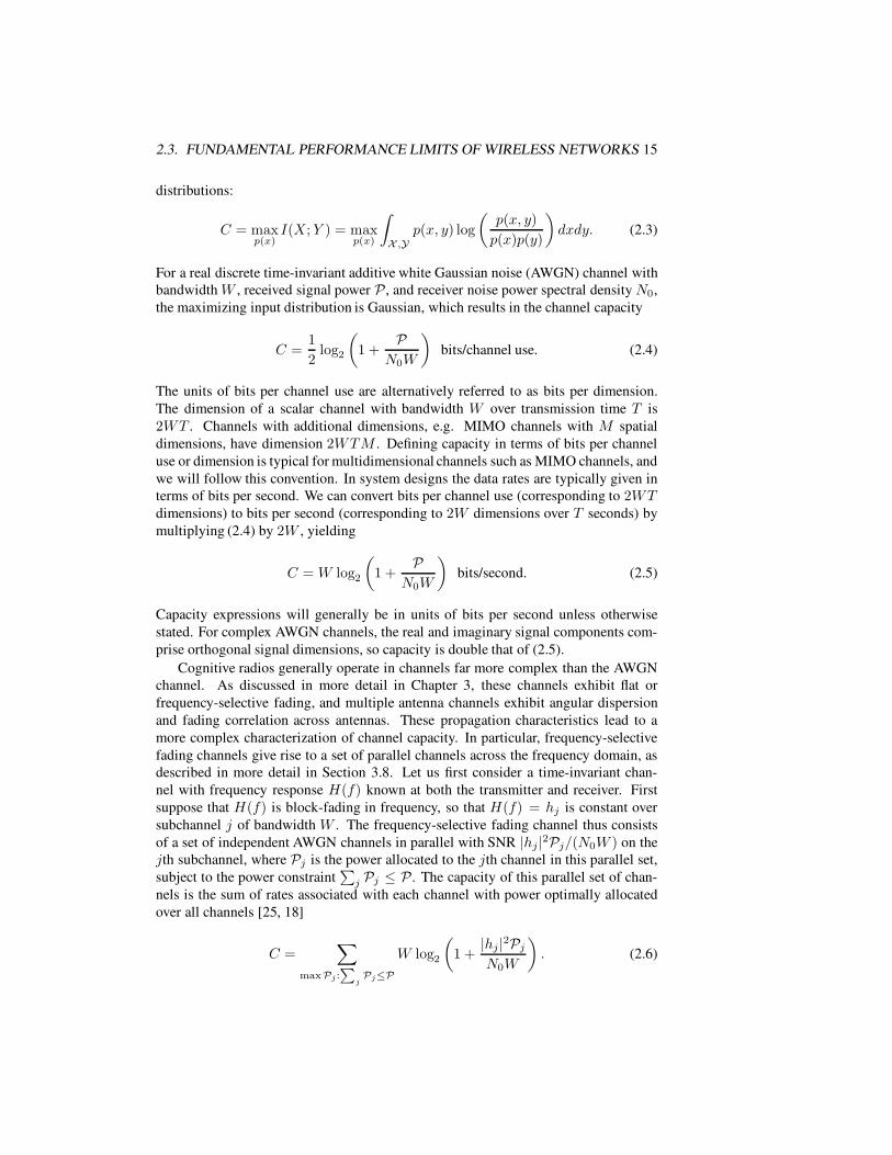
For a real discrete time-invariant additive white Gaussian noise (AWGN) channel with
bandwidth W , received signal power P, and receiver noise power spectral density N0,
the maximizing input distribution is Gaussian, which results in the channel capacity
C =1
2log2
(
1 +P
N0W
)
bits/channel use. (2.4)
The units of bits per channel use are alternatively referred to as bits per dimension.
The dimension of a scalar channel with bandwidth W over transmission time T is
2WT . Channels with additional dimensions, e.g. MIMO channels with M spatial
dimensions, have dimension 2WTM . Defining capacity in terms of bits per channel
use or dimension is typical for multidimensional channels such as MIMO channels, and
we will follow this convention. In system designs the data rates are typically given in
terms of bits per second. We can convert bits per channel use (corresponding to 2WTdimensions) to bits per second (corresponding to 2W dimensions over T seconds) by
multiplying (2.4) by 2W , yielding
C = W log2
(
1 +P
N0W
)
bits/second. (2.5)
Capacity expressions will generally be in units of bits per second unless otherwise
stated. For complex AWGN channels, the real and imaginary signal components com-
prise orthogonal signal dimensions, so capacity is double that of (2.5).
Cognitive radios generally operate in channels far more complex than the AWGN
channel. As discussed in more detail in Chapter 3, these channels exhibit flat or
frequency-selective fading, and multiple antenna channels exhibit angular dispersion
and fading correlation across antennas. These propagation characteristics lead to a
more complex characterization of channel capacity. In particular, frequency-selective
fading channels give rise to a set of parallel channels across the frequency domain, as
described in more detail in Section 3.8. Let us first consider a time-invariant chan-
nel with frequency response H(f) known at both the transmitter and receiver. First
suppose that H(f) is block-fading in frequency, so that H(f) = hj is constant over
subchannel j of bandwidth W . The frequency-selective fading channel thus consists
of a set of independent AWGN channels in parallel with SNR |hj|2Pj/(N0W ) on the
jth subchannel, where Pj is the power allocated to the jth channel in this parallel set,
subject to the power constraint∑
j Pj ≤ P. The capacity of this parallel set of chan-
nels is the sum of rates associated with each channel with power optimally allocated
over all channels [25, 18]
C =∑
maxPj:∑
jPj≤P
W log2
(
1 +|hj|2Pj
N0W
)
. (2.6)

16
The optimal power allocation is found by solving the Lagrangian, which leads to the
optimal power allocation
Pj
P =
{ 1γ0
− 1γj
γj ≥ γ0
0 γj < γ0(2.7)
for some cutoff value γ0, where γj = |hj|2P/(N0W ) is the SNR associated with
the jth subchannel assuming it is allocated the entire power budget. This optimal
power allocation is referred to as water-filling over frequency, whereby water (power)
is poured into a bowl of variable depth 1/γj up to the water line 1/γ0. Hence, more
power is allocated to subchannels with higher gains above the cutoff value γ0, which is
dictated by the power constraint. The capacity with this optimal power allocation then
becomes
C =∑
j:γj≥γ0
W log2(γj/γ0). (2.8)
This capacity is achieved by sending at different rates and powers over each subchan-
nel, similar to adaptive techniques used in OFDM. When H(f) is continuous the ca-
pacity under power constraint P is similar to the case of the block-fading channel with
the sum over subchannel capacities replaced by an integral of incremental capacity per
frequency over the frequency domain; details can be found in [25, Chapter 8.5][42].
Let us now consider multiple-input multiple-output (MIMO) channels, for which
the channel input is a random vector X = (X1, . . . , XMt) sent from the Mt transmit
antennas, the channel output is the vector Y = (Y1, . . . , YMr) obtained at the Mr re-
ceive antennas, and the channel is characterized by an Mt × Mr matrix H of gains
between each transmit and receive antenna. The multiple dimensions associated with
MIMO channel inputs and outputs give rise to the multiple spatial degrees of free-
dom over which independent data streams can be transmitted. Assuming the channel
is known at both the transmitter and receiver, capacity is achieved by optimizing the
transmit power and rate allocation across these spatial degrees of freedom. Specifically,
when the channel H is constant and known perfectly at the transmitter and receiver, the
capacity (maximum mutual information) in units of bits per channel use is
C = maxQ : tr(Q)=P
log2 det(
IN + HQHH)
(2.9)
where the optimization is over the input covariance matrix Q, which is Mt × Mt and
must be positive semi-definite by definition. Using the singular value decomposition
(SVD) of H, the MIMO channel can be converted into RH = rank(H) spatially paral-
lel, non-interfering single-input/single-output channels [84][32]. The jth spatial chan-
nel corresponding to singular value σj has SNR γj = |σj|2Pj/(N0W ), where power
Pj is optimally allocated across these spatial channels similar to the case of frequency
selective fading, which results in a water-filling power allocation over the spatial do-
main. The capacity formula is the same as in the frequency-selective fading case, given
by (2.8): the sum of capacities across the parallel spatial channels with this optimal
power allocation based on SNR per spatial dimension γj .
For time-varying channels, ergodic capacity is defined based on the channel state
distribution p(s) for both scalar and matrix channels. Specifically, the ergodic capacity

2.3. FUNDAMENTAL PERFORMANCE LIMITS OF WIRELESS NETWORKS 17
of a time-varying channel with instantaneous channel knowledge at both the transmitter
and receiver is given by
Cerg =
∫
s∈Sc
maxxs
C(s, xs)p(s)ds, (2.10)
where Sc is the set of all possible channel states, C(s, xs) is the capacity of a channel
in state s with input x, p(s) is the probability of state s, and xs is the channel input
for state s. These channel inputs are based on optimal allocation of transmit power
over time, subject to an average power constraint. For example, consider a flat-fading
channel, where the instantaneous SNR γ varies with time according to a distribution
p(γ). A discussion of fading distributions p(γ) under different conditions can be found
in Section 3.6. If the transmit power P(γ) is adapted relative to γ, subject to an average
power constraint P , then the flat-fading channel capacity is given by
C = maxP(γ):
∫
P(γ)p(γ)dγ=P
∫ ∞
0
W log2
(
1 +P(γ)γ
P
)
p(γ)dγ. (2.11)
The optimal power allocation P(γ) is found by solving the Lagrangian, similar to the
case of frequency selective fading. This yields optimal power allocation as a water-
filling over time:
P(γ)
P =
{
1γ0
− 1γ
γ ≥ γ0
0 γ < γ0(2.12)
for some “cutoff” value γ0 which is found via the average power constraint. If γ(t) is
below this cutoff at time t then no data is transmitted at that time. With this optimal
power allocation, the capacity of the time-varying flat-fading channel becomes
C =
∫ ∞
γ0
W log2
(
γ
γ0
)
p(γ)dγ, (2.13)
where the rate corresponding to instantaneous SNR γ is W log2(γ/γ0). Since γ0 is
constant, this means that as the instantaneous SNR increases, the data rate sent over the
channel for that instantaneous SNR also increases.
There is a strong similarity between time-varying flat-fading channels, MIMO chan-
nels, and time-invariant frequency-selective fading channels in that these channels can
be represented as a set of independent parallel channels in time, space, or frequency,
respectively. This property can be exploited in cognitive radio paradigms, in particu-
lar the interweave paradigm. Specifically, if the cognitive radio can sense that a given
dimension in time, space, or frequency is not being utilized by the primary user, it
can occupy that dimension with no harm to the primary system. The capacity analy-
sis for interweave systems is based on this concept, whereby the interweave cognitive
radio channel is modeled as a channel varying over time, frequency, or space. When a
given dimension is occupied by the primary user, under perfect sensing the interweave
channel in that dimension is unavailable to the cognitive radio, i.e. it is assumed to
have an SNR of zero. The capacity analysis above for parallel channels in time, space,
or frequency can then be applied directly to determine the capacity of the interweave
cognitive radio, as described in more detail in Chapter 2.6.

18
Figure 2.9: Wireless network model.
Capacity of multiuser channels and wireless networks are also built upon notions
of mutual information. However, the encoding and decoding strategies and their as-
sociated mutual information become more complicated with multiple users, and hence
the capacity regions are typically defined by a set of mutual information bounds that
implicitly define the capacity region boundary. Before launching into capacity results
for the different cognitive radio paradigms, we will first review capacity results for the
interference channel. Since, as discussed in Sec. 2.3.1, cognitive radio networks are all
special cases of the interference channel in Fig. 2.7, the capacity region and optimal
encoding and decoding strategies of the interference channel will provide fundamental
building blocks for obtaining capacity and design insights for cognitive networks.
2.3.3 Capacity Region of Wireless Networks
We consider a wireless network consisting of K source-destination pairs communicat-
ing over a common wireless channel, as shown in Fig. 2.9. We assume a discrete-time
network model with discrete channel inputs and outputs. At each time instant, a source
sk chooses a channel input Xk from a finite set Xk of possible inputs. Each destination
node dj observes a channel output Yj from output set Yj . The channel is described by
the conditional distribution p(y1, . . . , yK |x1 . . . xK), which characterizes the proba-
bility of the given set of outputs (y1, . . . , yK) at the destinations, for the given set of
channel inputs (x1, . . . , xK). A source sk wishes to communicate a data sequence or
message Wk ∈ Wk = {1, . . . , 2nRk} to destination dk , at rate Rk. To do so, the source
encoder maps the data sequence into a codeword Xn consisting of n symbols from the
input alphabet, and sends it in n time instants over the channel. All data sequences are
mutually independent. Upon receiving the sequence Y nj of length n, decoder j maps
it to its estimate of the transmitted data sequence, denoted by Wj . The data sequence
sets W1,W2, . . . ,WK along with the encoder and decoder mappings of all users define
an (R1, R2, . . . , RK, n) code for this channel. The encoding function at source sk for
data sequence Wk at time i is given as:
Xki = fk,i(Wk, Y i−1k ), k = 1, . . . , K. (2.14)
Note that the encoding function fk,i(·) allows the source to use its receiver’s previ-
ous observations of the channel (typically obtained via feedback) to encode Wk. This

2.3. FUNDAMENTAL PERFORMANCE LIMITS OF WIRELESS NETWORKS 19
allows sources to obtain information about data sequences sent by other users and po-
tentially forward them through the network. The decoding function at destination j at
time i is given as:
Wj = gj(Ynj ), j = 1, . . . , K. (2.15)
A decoding error at destination k occurs when Wk 6= Wk . We consider that an error
occurs unless all destinations decode their data sequences correctly. Thus, the error
probability is given by the probability of the union of error events associated with
incorrect detection on each of the different data sequences:
Pe = p
[
K⋃
k=1
[
Wk 6= Wk
]
]
. (2.16)
If the error probability can be made arbitrarily small for a code of sufficiently large n,
the rates (R1, . . . , RK) will be simultaneously achievable in the considered network.
More precisely, rates (R1, R2, . . . , RK) are achievable if, for any ε > 0, there exists,
for sufficiently large n, an (R1, R2, . . . , RK, n) code such that Pe ≤ ε. The capacity
region is the closure of the set of all achievable rates (R1, R2, . . . , RK), due to time-
sharing between strategies associated with any set of points on the rate region.
The above formulation assumes a single destination for each data sequence. This
definition can be extended to include multicasting to a set of destinations, broadcasting
from one source to a set of destinations or multiple access from multiple sources to
a single destination. The capacity region of a general wireless network is unknown.
A general outer bound to the network performance is provided by the cut-set bound
[18, 2, 26, 79], stated next.
Let S denote a subset of all network nodes and Sc be a complement of S. The pair
(S,Sc) is a cut separating source sk and destination dk if source sk ∈ S and dk ∈ Sc.
Cut-set outer bound; Any achievable (R1, . . . , RK) satisfies
∑
sk∈S,dk∈Sc
Rk ≤ I(X(S); Y (S) | X(Sc)), (2.17)
where mutual information is evaluated for some distribution p(x1, . . . , xK) for any S.
Rk is the rate across the cut from source sk to destination dk. We observe that (2.17)
bounds the sum rate going across a cut by the conditional mutual information between
all sources in S and all destinations in Sc, given all sources in Sc.
As an example of the cut-set outer bound, consider K source–destination pairs with
AWGN links of bandwidth W . The channel inputs and outputs are then vectors defined
by
Y = HX + Z (2.18)
where X is the vector of channel inputs from all the sources with average power con-
straint P, Y is the vector of all channel outputs, H ∈ RK×K is the channel gain matrix
and Z is the vector of independent, unit-variance Gaussian noises at the destinations.
The cut-set bound in (2.17) evaluates to [27]∑
sk∈S,dk∈Sc
Rk ≤ W log2 det(
I + H(S)K(S)H(S)T)
(2.19)

20
where I is the identity matrix, K(S) is the covariance matrix of X(S) given X(Sc),and H is determined such that
Y(Sc) = H(S)X(S) + HT (S)X(Sc) + Z(Sc). (2.20)
As another example of the cut-set outer bound, consider the three-node relay chan-
nel shown in Fig. 2.7. Assume that links are AWGN links of bandwidth W . Let Xs
denote the symbol sent from the source, and Xr denote the symbol sent from the relay.
Source and relay powers are denoted by Ps and Pr . The received symbols at the desti-
nation and the relay, respectively, are Yd and Yr. There are two cuts in the network: in
the first cut, only the source forms the set S, whereas in the second cut the source and
the relay form the set S. The cut-set bound (2.17) evaluates to
R ≤ maxp(xs,xr)
min{I(Xs; Yr, Yd|Xr)I(Xs, Xd; Yr)} . (2.21)
In the AWGN relay channel this yields
R ≤ max0≤ρ≤1
min
{
W log2
(
1 + Ps + Pr + 2ρ√
PsPr
)
,1
2
(
1 + (Ps + Pr)(1 − ρ2))
}
,
(2.22)
where we normalize the noise power to one. The parameter ρ determines the correlation
between inputs Xs and Xr. A larger ρ corresponds to a larger coherent combining gain.
The cut-set bound is a tight outer bound only for certain special scenarios. In
general, the cut-set bound is loose relative to the network capacity region. Alternative
outer bounds to the cut-set outer bound can be derived by using genie-based techniques
in which the network is modified by assuming that additional information is known
(a.k.a., given by a genie) to a subset of terminals. The goal of providing this information
is to obtain a modified network for which capacity or an outer bound can be obtained.
Due to the additional information, the modified network outperforms the original one.
Consequently, its capacity (or any outer bound on it) yields a capacity outer bound
for the original network. Outer bounds can also be obtained by the theory of network
equivalence [50]. This approach provides conditions under which the capacity of a
wireless network can be upper bounded by the performance of an equivalent noiseless
network of bit pipes, for which the capacity can then be determined. Another technique
to tighten the cut-set bound is by modification of the network connectivity graph [53,
54].
Obtaining the Shannon capacity region of a wireless network is generally intractable;
in fact the capacity of several simple canonical topologies such as the relay channel and
the interference channel have remained open problems for decades. As an alternative
capacity metric, a landmark result by Gupta and Kumar [38] introduced the notion of
scaling laws for noncognitive wireless network throughput as the number of nodes in
the network K grows asymptotically large. They found that the throughput in terms
of bits per second for each node in the network decreases with K at a rate between
1/√
K logK and 1/√
K . In other words the per-node rate of the network goes to zero,
although the total network throughput, equal to the sum of rates, grows at a rate be-
tween√
K/ logK and√
K. This surprising result indicates that when interference
is treated as noise (as is typical in practical designs), even with optimal routing and

2.4. INTERFERENCE CHANNELS WITHOUT COGNITION 21
scheduling, the per-node rate in a large ad hoc wireless network goes to zero. The
reason is that in this relatively simple relaying scheme, intermediate nodes spend much
of their resources forwarding packets for other nodes, so few resources are left to send
their own data. There has been much follow-on work to this result, including the im-
pact on wireless network scaling laws of mobility, multiple antennas, and cooperation
[36, 5, 68]. In particular, [68] showed that more sophisticated cooperation schemes
allow per-node rates in large networks to remain constant with network size rather than
decrease. The tradeoff between throughput (in terms of scaling laws) and delay in
asymptotically large networks was characterized in [39, 86, 22].
2.4 Interference Channels Without Cognition
2.4.1 K-user Interference Channels
In cognitive radio networks, we would like to characterize capacity associated with
communications between primary user pairs and between secondary user pairs. Al-
though one could envision deployment of relays to improve the performance, these
networks typically do not involve multihop routing of information, i.e., there is no
forwarding of information through intermediate nodes. Without cognition, networks
with K source-destination pairs can be modeled as a K-user interference channel, as
shown in Fig. 2.10. Although the capacity region of this channel is in general unknown,
there has been a lot of progress in understanding how to cope with interference in this
model and, consequently, in developing spectrally-efficient transmission schemes for
this channel. In some scenarios, these techniques lead to capacity. A cognitive radio
network forms a two-tier K-user interference channel, due to the different capabilities
and restrictions of primary and secondary users. Schemes that efficiently cope with
interference can improve performance of both primary and secondary users in these
networks. For that reason, some of the techniques developed for interference chan-
nels have been adopted for overlay cognitive networks as well. We next review these
techniques, their performance and their known capacity results. In addition, cognition
enables additional encoding/decoding techniques to improve the performance. Hence,
performance of interference channels can serve as a lower bound to the capacity of
cognitive networks.
In the K-user interference channel model, each of the K sources wishes to commu-
nicate with its corresponding destination over a shared wireless channel, as illustrated
in Fig. 2.10. Source sk encodes and sends a data sequence Wk at rate Rk to destination
dk. The K-user interference channel is a special case of a K-user wireless network,
and hence we use the same definitions as in Chapter 2.3.1 for encoding, decoding, er-
ror probability, and capacity. However, the encoding function of the kth user in the
interference channel is given by
Xnk = fk(Wk). (2.23)
Thus, in this case a channel input at each source depends only on its own data sequence,
which, in turn, is independent of data sequences from other sources. Hence, there is

22
Figure 2.10: K-user interference channel. Sender k wishes to communicate to desti-
nation k.
no cooperation (e.g. relaying) between sources in transmitting information about each
other’s data sequences. The cut-set bound (2.17) can then be tightened to become
∑
sk∈S,dk∈Sc
Rk ≤ I(X(S); Y (S)|X(Sc), V ) (2.24)
for any p(v)∏
k p(xk|v) where V , referred to as a time-sharing random variable, has
the property that the inputs {xk} are independent when conditioned on v,
Lower bounds to the capacity region are obtained by deploying specific communi-
cation techniques in the given network. We next present encoding schemes that achieve
capacity for special cases of the two-user interference channel.
2.4.2 Two-user Interference Channel Capacity
Figure 2.11: Two-user interference channel.

2.4. INTERFERENCE CHANNELS WITHOUT COGNITION 23
A two-user discrete-time memoryless interference channel is shown in Fig. 2.11.
The interference channel contains only two communicating pairs (K = 2). Therefore,
there are two channel inputs X1 and X2, and two channel outputs, Y1 and Y2. The
discrete-time channel is characterized by the conditional distribution p(y1, y2|x1, x2).Each source sk , k = 1, 2, wishes to send a data sequence Wk ∈ W = {1, . . . , 2nRk} to
destination dk. Definitions for the channel code, the error probability and the capacity
region follow the definitions for the K-user interference channel. In particular, an
(R1, R2, n) code consists of two data sequence sets W1,W2, two encoding functions
Xn1 = f1(W1) (2.25)
Xn2 = f2(W2) (2.26)
and two decoding functions
Wk = gk(Y nk ), k = 1, 2. (2.27)
The error probability of the code is
Pe,k = P[[
W1 6= W1
]
⋃
[
W2 6= W2
]]
. (2.28)
A rate pair (R1, R2) is achievable if, for any ε > 0, there exists for sufficiently large nan (R1, R2, n) code such that Pe ≤ ε. The capacity region of the interference channel
is the closure of the set of all achievable rate pairs (R1, R2).We will also consider the AWGN interference channel, defined by the input–output
relation:
Y1 = X1 + aX2 + Z1
Y2 = bX1 + X2 + Z2 (2.29)
where a and b are real numbers representing cross-channel gains, E[X2k ] ≤ Pk are
power constraints, and Zk ∼ N(0, 1) for k = 1, 2 where N(0, σ2) denotes the Gaussian
distribution with variance σ2.The capacity of the interference channel is known in strong interference [15]. In
this regime, the interfering signal at each receiver is strong enough so that the other
user’s data sequence carried by that signal can be decoded and hence removed. It is then
optimal for each receiver to decode both data sequences. In the AWGN interference
channel (2.29), the strong interference conditions are given by [74, 40]
|a| ≥ 1
|b| ≥ 1 (2.30)
implying that in this regime the cross-channel gains are larger than the direct link gains.
In general discrete memoryless channel, the strong interference conditions can be
expressed in terms of the conditional mutual information inequalities. These conditions
require that
I(X1 ; Y1|X2) ≤ I(X1; Y2|X2) (2.31)
I(X2 ; Y2|X1) ≤ I(X2; Y1|X1) (2.32)
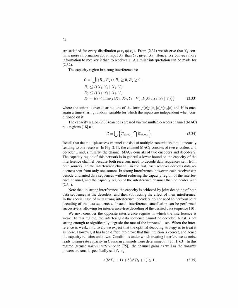
24
are satisfied for every distribution p(x1)p(x2). From (2.31) we observe that Y2 con-
tains more information about input X1 than Y1, given X2. Hence, X1 conveys more
information to receiver 2 than to receiver 1. A similar interpretation can be made for
(2.32).
The capacity region in strong interference is:
C =⋃
{(R1, R2) : R1 ≥ 0, R2 ≥ 0,
R1 ≤ I(X1 ; Y1 | X2, V )
R2 ≤ I(X2 ; Y2 | X1, V )
R1 + R2 ≤ min{I(X1 , X2; Y1 | V ), I(X1, X2; Y2 | V )}} (2.33)
where the union is over distributions of the form p(v)p(x1 |v)p(x2|v) and V is once
again a time-sharing random variable for which the inputs are independent when con-
ditioned on it.
The capacity region (2.33) can be expressed via two multiple-access channel (MAC)
rate regions [18] as:
C =⋃
{
RMAC1
⋂
RMAC2
}
. (2.34)
Recall that the multiple access channel consists of multiple transmitters simultaneously
sending to one receiver. In Fig. 2.11, the channel MAC1 consists of two encoders and
decoder 1 and, similarly, the channel MAC2 consists of two encoders and decoder 2.
The capacity region of this network is in general a lower bound on the capacity of the
interference channel because both receivers need to decode data sequences sent from
both sources. In the interference channel, in contrast, each receiver decodes data se-
quences sent from only one source. In strong interference, however, each receiver can
decode unwanted data sequences without reducing the capacity region of the interfer-
ence channel, and the capacity region of the interference channel then coincides with
(2.34).
Note that, in strong interference, the capacity is achieved by joint decoding of both
data sequences at the decoders, and then subtracting the effect of their interference.
In the special case of very strong interference, decoders do not need to perform joint
decoding of the data sequences. Instead, interference cancellation can be performed
successively, allowing for interference-free decoding of the desired data sequence [10].
We next consider the opposite interference regime in which the interference is
weak. In this regime, the interfering data sequence cannot be decoded, but it is not
strong enough to significantly degrade the rate of the impacted user. When the inter-
ference is weak, intuitively we expect that the optimal decoding strategy is to treat it
as noise. However, it has been difficult to prove that this intuition is correct, and hence
the capacity remains unknown. Conditions under which treating interference as noise
leads to sum-rate capacity in Gaussian channels were determined in [75, 1, 63]. In this
regime (termed noisy interference in [75]), the channel gains as well as the transmit
powers are small, specifically satisfying:
a(b2P1 + 1) + b(a2P2 + 1) ≤ 1. (2.35)

2.4. INTERFERENCE CHANNELS WITHOUT COGNITION 25
The sum-rate capacity is then given by [75, Theorem 2]
C = W log2
(
1 +P1
1 + a2P2
)
+ W log2
(
1 +P2
1 + b2P1
)
. (2.36)
The proof of this result required a genie-based outer bound for the Gaussian interfer-
ence channel.
The above described regimes are two extremes with respect to the amount of in-
terference that is being experienced and removed by receivers. Not surprisingly, in
strong interference the highest-rate scheme is to decode the unwanted data sequences
and subtract their corresponding signals, thus removing their interference from the re-
ceived signal. In the other extreme of weak interference, the highest-rate strategy is to
ignore the interference, that is, treat it as noise.
In regimes that are in between the two extremes, the interference is not strong
enough so that decoding of the unwanted data sequence is optimal, nor it is weak
enough to be treated as noise without loss of optimality. In this scenario, decoding
part of an interfering data sequence to partially remove interference from the received
signal is beneficial. This idea is realized in the scheme developed by Carleial and sub-
sequently improved by Han and Kobayashi, also referred to as rate-splitting [11, 40].
The rate-splitting concept is illustrated in Fig. 2.12. To perform rate-splitting, each
encoder divides its data sequence into two data sequences, each of lower rate than the
original sequence, and encodes them via superposition coding. In this superposition
coding, the source encodes each of the two data sequences using a separate codebook,
divides its transmit power between the two (in the case of the AWGN interference chan-
nel), and adds them together to obtain the channel input. Separate encoding enables a
receiver to decode one data sequence intended for the other user jointly with its own
data sequence, while treating the signal carrying the other part of the undesired data
sequence as noise. The communication rate for this user increases due to reduced in-
terference, but the rate for the other communicating pair decreases due to an additional
decoding constraint. Hence, there is a tradeoff between the amount of information sent
only to the desired receiver and the amount of interference decoded at the other one.
In AWGN interference channels, this encoding tradeoff translates into optimizing
the power allocated to each of the two parts of the encoder’s data sequence. By choos-
ing Gaussian codebooks, , i.e. random codebooks generated according to a Gaus-
sian distribution, and a specific power split, the Han-Kobayashi scheme achieves rates
within one bit per dimension from the two-user interference channel capacity [23].
The power split is chosen so that the created interference at each receiver has the same
power as the Gaussian noise at that receiver. Thus, the created interference is suf-
ficiently weak so as not to significantly impair performance. At the same time, the
undesired data sequence that is decoded at each destination allows for significant inter-
ference reduction. In Section 2.7 we will give more details on how rate splitting can be
used in overlay cognitive radio networks.
In a K-user interference channel, each receiver is exposed to interference arriving
from multiple sources. A generalization of the Han-Kobayashi scheme would allow
for partial decoding of each interfering signal. A receiver could then jointly decode its
own data sequence along with some portion of the interfering data sequences dictated

26
Figure 2.12: Rate splitting. Each encoder splits its message into two messages of lower
rate encoded via superposition coding. A decoder jointly decodes one message of the
other user together with its desired message.
by the rate-splitting code design. While such a generalization is possible mathemati-
cally, it would result in very complex encoding and decoding schemes at each node.
Specifically, this approach requires a receiver to separately decode parts of interfering
data sequences sent from many interferers in order to reduce interference. Instead, the
interference at each receiver can be treated collectively in a more efficient manner via
interference alignment [7, 58] or via structured codes [65]. These approaches exploit
the fact that a receiver is not interested in information associated with interfering data
sequences and hence does not need to decode them (or parts of them). Interference
alignment achieves the optimal capacity scaling law in the interference channel [69].
Lattice codes outperform the Han-Kobayashi scheme in the K-user interference chan-
nel [83].
The AWGN channel considered so far in this section assumes constant channel
coefficients and hence does not capture flat or frequency-selective fading. Incorpo-
rating these channel characteristics leads in general to channel models that are more
difficult to analyze. However, these characteristics open up possibilities for encoding
and transmission strategies that exploit fading. In particular, frequency-selective and
time-varying channels can be modeled as parallel interference channels [8]. Results
in [8] demonstrate that parallel interference channels are optimized by joint encoding
across subchannels. This is in contrast to point-to-point, multiple access and broadcast
parallel channels in which separate encoding over the subchannels is optimal. Further
exploration of K-user interference channels has revealed that time-variations can be
exploited to combat interference in the form of interference alignment. Interference
alignment relies on channel time-variations to achieve half of the interference-free ca-
pacity for each user in the system [7, 66].
2.4.3 Interference Channel Techniques for Cognitive Radios
In interference networks with no cognition, a plausible transmission scheme to avoid
interference is to split the bandwidth and assign orthogonal channels to each com-

2.5. UNDERLAY COGNITIVE RADIO NETWORKS 27
municating pair, e.g., via a MAC protocol that divides channels orthogonally in time,
frequency or space. In cognitive radio networks, this corresponds to the interweave ap-
proach to avoid interference between cognitive and primary users. However, in general,
dividing the bandwidth orthogonally reduces spectral efficiency in comparison with as-
signing the full bandwidth to all users and then coping with the introduced interference.
One exception is in the low-SNR regime where the network is power-limited rather than
interference-limited. In this regime, bandwidth is plentiful compared to power, and thus
assigning orthogonal channels to users incurs no performance loss. In the interference-
limited regime this is no longer true. Furthermore, as the number of network users
increases, the rate per user of an orthogonal MAC scheme goes to zero. This reason-
ing emphasizes why the overlay approach may be a more spectrally-efficient technique
for cognitive radios than the interweave approach. We analyze capacity regions of the
interweave and the overlay cognitive radio in Sections 2.6 and 2.7, respectively.
Rate-splitting and superposition coding can also be applied to treat interference in
overlay cognitive radio networks. An overlay cognitive radio shares its bandwidth with
one or more primary users, thereby creating interference at the primary receivers. At
the same time, the secondary receivers experience interference from the primary user
transmissions. Efficiently coping with interference can thus improve the performance
of both secondary and primary users in the system. We will see that in overlay cognitive
radio systems there exists a regime of strong interference in which decoding of the
unwanted data sequences is optimal. Similarly, there is a weak interference regime in
which interference can be treated as noise without loss of optimality.
Furthermore, cognitive capabilities enable radios to deploy transmission strategies
that cannot be deployed in interference channels without cognition. By listening to the
channel, a secondary user can obtain information about primary user data sequences,
assuming the security and privacy concerns of the primary system can be addressed.
Given this information, the secondary user can cooperate with the primary user. By
relaying the information (or a part of it) to the primary receiver, the secondary user can
improve the quality of reception and thus the rate for the primary user. Alternatively,
the secondary user can allocate a part of its power to relay the primary data sequence
and the rest of its power to transmit its own information. The power split should be
chosen such that the resulting SINR ratio at the primary receiver yields the same rate
performance as if the secondary user was not present.
In summary, when compared to wireless networks with no cognition, a cognitive
radio can cope with interference using techniques developed for interference channels.
In addition, cognition enables the secondary encoder to protect its own information
from the interference caused by the primary system by precoding against interference.
These techniques will be described in more detail in Section 2.7.
2.5 Underlay Cognitive Radio Networks
The underlay approach to cognitive radio allows for spectrum sharing between pri-
mary and secondary users, under the constraint that the interference caused by sec-
ondary users does not noticeably degrade the performance of the primary users. When
the performance of a primary user is measured by its SINR in each signal dimension,

28
the total interference that secondary users cause to any primary user is typically con-
strained to be within a given spectral mask, i.e. a limit on the power spectral density
of the interference over frequency and, for MIMO channels, over space. The interfer-
ence constraint, in turn, imposes a constraint on the total power spectral density per
dimension received from all secondary transmitters at any primary receiver. In order to
satisfy the interference constraint, several different conditions can be imposed on the
secondary transmission. Interference caused by secondary transmissions can be lim-
ited by imposing an average received power per dimension constraint or a peak received
power per dimension constraint at the primary user. When primary and secondary users
experience time-varying channels, the primary users’ performance requirements may
be based on meeting a given interference constraint at each time instant or an average
interference power constraint over time. An alternative underlay paradigm does not im-
pose constraints on interference but rather on the minimum value of the primary user’s
capacity. However, this is not a common paradigm since it is simpler for a secondary
user to determine the interference it causes to a primary receiver than to determine the
capacity degradation it causes. Thus, we will focus on capacity of underlay systems
under interference constraints imposed on the secondary users.
When multiple secondary and primary users coexist, their interference constraint
needs to be satisfied at the primary user that is the most impaired by the interference
from secondary users. As explained earlier, satisfying the interference condition re-
quires that a secondary transmitter knows the channel to the primary receiver. Other-
wise, in order to guarantee that the interference constraint is satisfied under unknown
channel conditions, the secondary user’s transmit power needs to be severely restricted.
In the presence of multiple secondary users, determining the interference at the primary
receiver becomes more demanding, as the interference depends on transmit powers and
channel conditions from all secondary transmitters, as described in more detail later in
this section.
2.5.1 Underlay Capacity Region
The capacity region of the underlay cognitive radio network can be defined following
the capacity definition for wireless ad hoc networks, while taking into account the
interference constraints at the primary users as well as the channel characteristics. To
define the received power constraint, we consider first a narrowband system with one
secondary and one primary user, as shown in Fig. 2.13. We extend this to networks with
multiple primary and secondary users below. In this two-user network, an interference
constraint translates to a received power constraint on the secondary user’s signal at
the primary user’s receiver. Let Xi denote the channel input at time i by the secondary
user and Yi denote the corresponding channel output at the primary receiver. The
channel between the secondary transmitter and the primary receiver is assumed to be
memoryless and hence can be described by a conditional probability distributionp(y|x)at each time i, as illustrated in Fig. 2.13 for the link between the secondary transmitter
and primary receiver. With each input-output pair (x, y), we associate a cost function
c(x, y). The average cost function over n transmissions is then defined as the average

2.5. UNDERLAY COGNITIVE RADIO NETWORKS 29
of the per-symbol cost:
E[cn(Xn , Y n)] =1
n
n∑
i=1
E[c(Xi, Yi)], (2.37)
where the expectation is with respect to Xi and Yi. The interference constraint is based
on imposing a maximum value for this average cost:
E[cn(Xn , Y n)] ≤ η (2.38)
The average received power constraint is a special case of (2.38), where a constraint
is imposed only on the received signal and the cost function is chosen to be c(y) = |y|2:
1
n
n∑
i=1
E
[
|Yi|2 | Xi
]
≤ η. (2.39)
Note that the constraint (2.39) is based on requiring that the average power of the re-
ceived interference plus noise falls below η; to obtain the corresponding interference
constraint, the noise power must be subtracted from η. The received peak power con-
straint,indexconstraint!received peak power based on a per symbol constraint, is given
by
E
[
|Yi|2 | Xi
]
≤ ηpeak i = 1, . . . , n. (2.40)
When the channel is static, the channel and corresponding input distribution on Xi is
the same for all i, so the average and peak power constraints are the same, given by
(2.40) with η = ηpeak. When the channel is wideband such that the received power
constraint is defined by a spectral mask over frequency, the average and peak power
constraint definitions can be extended to constraints on average or peak power spectral
density over frequency. The capacity region can then be defined equivalently to the
capacity region of the wireless network while taking into account the average or peak
received power constraint, as we now describe in more detail. In this development we
will assume a narrowband channel with average or peak power constraints given by
(2.39) or (2.40), but the results can be easily extended to wideband channels with a
spectral mask constraint by considering the received power spectral density over all
frequencies.
Let us now consider a network with K source-destination pairs communicating
over a common memoryless channel. The conditional distribution of the channel inputs
and outputs is given by p(y1, . . . , yK |x1, . . . , xK). We assume further that the network
contains Kp primary and Ks secondary pairs such that Kp + Ks = K. Each source
sk wishes to communicate to a corresponding destination dk at rate Rk, over n uses
of the channel. The code for the network, (R1, . . . , RK, n), is defined as before by
(2.14)-(2.15). The error probability of the code is given by (2.16). We denote the set of
primary receivers as SPR, and the set of secondary transmitters as SST.
Let Yi,j denote the interference at the jth primary receiver caused by all secondary
transmitted symbols Xi,m at time i, for m ∈ SST. Under an average power constraint,
we thus require that
1
n
n∑
i=1
E
[
|Yi,j|2 | {Xi,m, m ∈ SST}]
≤ η, ∀j ∈ SPR. (2.41)

30
Figure 2.13: Underlay system with single primary and secondary pair.
Condition (2.41) thus extends condition (2.39) to a K-user setting by requiring that the
average received interference power from all interfering secondary users is smaller than
threshold η at all primary receivers. Alternatively, a received peak power constraint at
each time i can be imposed as
E
[
|Yi,j|2 | {Xi,m, m ∈ SST}]
≤ ηpeak, i = 1, . . . , n, ∀j ∈ SPR. (2.42)
Rates (R1, . . . , RK) are achievable if, for any ε there exists an (R1, . . . , RK, n) code
such that Pe < ε and the constraint (2.41) is satisfied for the set SPR. The capacity
under the cost constraint is the closure of the set of the achievable rates since time-
sharing between different strategies can be used.
The capacity region will characterize the set of achievable rates for both primary
and secondary users. In underlay cognitive radio networks, the premise is that the
primary users’ performance is minimally affected by the presence of secondary users.
This impact on capacity can be approximated by modeling the secondary users as an
additional source of Gaussian noise with power given by the imposed received power
constraint. The capacity for secondary users can then be considered separately, under
the average or peak received power constraints, and treating the interference from the
primary system to the secondary system as noise. We now determine the capacity of
the secondary user system under these assumptions for several different channel and
network assumptions.
2.5.2 Capacity Results for Specific Scenarios
Single Secondary User: Static Scalar Channel
Suppose the secondary user transmits over a point-to-point static channel. Its input-
output relationship to the primary user’s receiver is then given by
Y = hX + Z (2.43)

2.5. UNDERLAY COGNITIVE RADIO NETWORKS 31
where h is the complex channel gain assumed known by the secondary user and Z ∼N [0, σ2] is additive white Gaussian noise with variance σ2. In our model this noise
consists of both receiver noise and the noise associated with the primary system. Since
the channel is static, the expected power of each transmitted symbol is the same. Hence,
the average received power constraint (2.39) for this channel is given by
E|Y |2 = |h|2E|X|2 + σ2 ≤ η. (2.44)
This can be translated to a transmit power constraint as
E|X|2 ≤ η − σ2
|h|2 . (2.45)
The capacity is then given by the capacity of the AWGN channel (2.5) with transmit
power constraint (2.45).
Single Secondary User: Static MIMO Channel
The static Gaussian MIMO channel is given by
Y = HX + Z (2.46)
where X ∈ CM , Y ∈ CN , H ∈ CN×M is the channel gain matrix and Z ∈ CN is the
vector of AWGN noise components at each receive antenna, where each component
has variance σ2. The capacity of this channel assuming the channel is known at the
transmitter and receiver and under a transmit power constraint was given by (2.8),
and equals the sum of capacities over each spatial channel with optimal spatial power
allocation via water-filling. Since this is also a static channel, the underlay average
received power constraint (2.39) corresponds to a received power constraint on the
vector Y = (Y1, . . . , YN) received at the primary user, which is given by
E[
||Y||2 | X, HSP
]
= ν + Nσ2 ≤ η, (2.47)
where Y = HSP X + Z for HSP the matrix of channel gains from the secondary
transmitter to the primary receiver. We have separated the received power constraint
into two components, ν and Nσ2, where the former is based on interference and the
latter based on noise. Thus, ν = ||HSPX||2. The received power constraint (2.47)
changes the capacity significantly as it precludes the optimal spatial water filling over
the matrix H of channel gains for the secondary user’s channel based on a transmit
power constraint. In particular, it was shown in [29, Sec. III] that the capacity of the
secondary user MIMO channel H under constraint (2.47) is
C = rank(H) log2
(
1 +ν
rank(H)σ2
)
, (2.48)
This capacity formula depends only on the rank of the secondary user’s channel H
matrix, rather than on its singular values as in (2.8), although the code that achieves the
capacity in (2.48) depends on the full matrix H and not just its rank.
Single Secondary User: Flat-Fading Channel

32
We next assume that the channel (2.43) is a flat-fading channel with random channel
gain h that varies over time. In this case, power should be optimally allocated over
time, and both the ergodic and outage capacity are performance metrics of interest. It
is shown in [31] that the ergodic capacity under the average received power constraint
imposed by the primary system yields
C =
∫ ∫
W log2
( |hs|2|h|2WN0λ
)
p(hs)p(h)dhsdh, (2.49)
where hs is the channel gain from the secondary transmitter to the secondary receiver.
The optimal power allocation in this case is given by
P ∗ =
(
1
λ|h|2 − N0W
|hs|2)+
, (2.50)
where λ is determined to satisfy the received power constraint as
∫ ∫(
1
λ− N0W
|h|2|hs|2
)+
p(hs)p(h)dhsdh = η. (2.51)
This optimal power allocation is similar to the time water-filling given by (2.12) un-
der a transmit power constraint. However, imposing a power constraint at the primary
receiver results in a time-varying water level inversely proportional to |h|2, the magni-
tude squared of the instantaneous time-varying channel gain. Moreover, the cutoff fade
depth below which no data is transmitted by the secondary user depends both on his
channel gain hs as well as the gain h between the secondary transmitter and primary
receiver. In particular, the secondary user increases his transmit power when either hs
increases (as his channel is better, i.e. conventional water-filling) or when h decreases,
since less interference is caused to the primary. Note that, from (2.49), the capacity
depends on channel statistics from the secondary transmitter to both primary and sec-
ondary receivers. Interestingly, it is shown in [31] that the capacity (2.49) when both
hs and h experience Rayleigh fading is larger than the capacity of the corresponding
AWGN channel with the same average SNR. However, with this Rayleigh fading on
both channels, the average SNR is low, and it is known that at low SNRs the ergodic
capacity of a Rayleigh fading channel exceeds that of an AWGN channel with the same
SNR [32, Figure 4.7]. Note, however, that this is in some sense an artifact of the in-
finitely long tail probability of the Rayleigh distribution, which results in a set of very
high SNR channels with very low probability. These rare high–SNR channels can be
exploited by allocating significant power and rate during these low probability events,
which results in a slightly higher capacity than a static channel maintaining a fixed
rate commensurate with the same average SNR. Note, also, that the propagation char-
acteristics which induce fading also cause some reduction in average received power.
Hence, comparing fading and nonfading channels with the same average SNR does not
fully capture the impact of fading on performance.
Under the peak constraint (2.40), the optimum power strategy for the secondary
user is simply to transmit at the highest power allowed by (2.40). The capacity is then
given by
C =
∫ ∫
W log
( |hs|2|h|WN0λ
)
p(hs)p(h)dhsdh. (2.52)
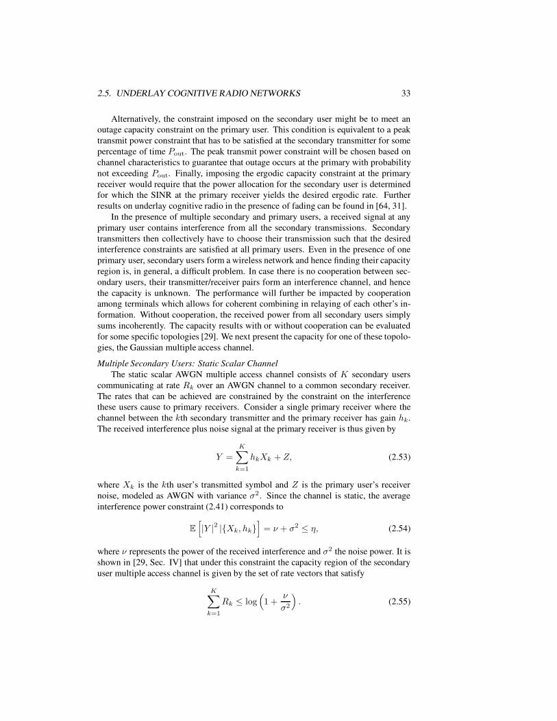
2.5. UNDERLAY COGNITIVE RADIO NETWORKS 33
Alternatively, the constraint imposed on the secondary user might be to meet an
outage capacity constraint on the primary user. This condition is equivalent to a peak
transmit power constraint that has to be satisfied at the secondary transmitter for some
percentage of time Pout. The peak transmit power constraint will be chosen based on
channel characteristics to guarantee that outage occurs at the primary with probability
not exceeding Pout. Finally, imposing the ergodic capacity constraint at the primary
receiver would require that the power allocation for the secondary user is determined
for which the SINR at the primary receiver yields the desired ergodic rate. Further
results on underlay cognitive radio in the presence of fading can be found in [64, 31].
In the presence of multiple secondary and primary users, a received signal at any
primary user contains interference from all the secondary transmissions. Secondary
transmitters then collectively have to choose their transmission such that the desired
interference constraints are satisfied at all primary users. Even in the presence of one
primary user, secondary users form a wireless network and hence finding their capacity
region is, in general, a difficult problem. In case there is no cooperation between sec-
ondary users, their transmitter/receiver pairs form an interference channel, and hence
the capacity is unknown. The performance will further be impacted by cooperation
among terminals which allows for coherent combining in relaying of each other’s in-
formation. Without cooperation, the received power from all secondary users simply
sums incoherently. The capacity results with or without cooperation can be evaluated
for some specific topologies [29]. We next present the capacity for one of these topolo-
gies, the Gaussian multiple access channel.
Multiple Secondary Users: Static Scalar Channel
The static scalar AWGN multiple access channel consists of K secondary users
communicating at rate Rk over an AWGN channel to a common secondary receiver.
The rates that can be achieved are constrained by the constraint on the interference
these users cause to primary receivers. Consider a single primary receiver where the
channel between the kth secondary transmitter and the primary receiver has gain hk.
The received interference plus noise signal at the primary receiver is thus given by
Y =
K∑
k=1
hkXk + Z, (2.53)
where Xk is the kth user’s transmitted symbol and Z is the primary user’s receiver
noise, modeled as AWGN with variance σ2. Since the channel is static, the average
interference power constraint (2.41) corresponds to
E
[
|Y |2 |{Xk, hk}]
= ν + σ2 ≤ η, (2.54)
where ν represents the power of the received interference and σ2 the noise power. It is
shown in [29, Sec. IV] that under this constraint the capacity region of the secondary
user multiple access channel is given by the set of rate vectors that satisfy
K∑
k=1
Rk ≤ log(
1 +ν
σ2
)
. (2.55)

34
Broadcast Channel
The broadcast channel consists of one secondary user communicating simultane-
ously with K receivers. Since there is only one secondary transmitter creating inter-
ference to a primary user, this case is equivalent to the case of the broadcast AWGN
channel (between the secondary transmitter and the primary receiver) with average
received power constraint. Thus, the total rate at which the secondary encoder can
transmit to all K receivers is given by the capacity of the corresponding point-to-point
AWGN channel with a transmit power constraint.
In fading channels, the constraint on average or peak received power, ergodic or
outage capacity can be considered as before. And while the capacity of networks of the
multiple secondary users capacity is in general unknown, the performance for specific
topologies can be evaluated under each of these constraints. For example, for a net-
work with multiple primary users and a single secondary user, the received peak power
constraint translates to multiple transmit peak power constraints at the secondary trans-
mitter. The optimal power allocation is then to choose the lowest peak power allowed
by these constraints.
2.6 Interweave Cognitive Radio Networks
The fundamental performance limits of interweave cognitive radios depend on assump-
tions about the overall system model as well as assumptions about the ability of the
cognitive radio system to sense the interference it causes to primary users. In some
cases these assumptions allow known capacity results or bounds to be applied. When
detection is imperfect, the impact of missed detection and false alarms of primary user
activity reduces capacity of both the secondary and primary users, and this loss of ca-
pacity must be formally characterized. In addition to capacity regions, scaling laws for
interweave cognitive networks will be presented for different models that indicate how
capacity scales as the number of secondary users grows.
This section focuses on the rate limits based on information-theoretic capacity of
interweave channels. Specifically, we discuss Shannon capacity, outage and ergodic
capacity, as well as scaling laws. In addition to these information-theoretic limits, per-
formance of interweave cognitive systems can also be limited by detection and hard-
ware constraints. In particular, interweave systems with poor sensing capability will
have high probabilities of missed detection and false alarm, which will significantly
degrade the performance of both the primary and secondary users. Similarly, the fre-
quency agility of the secondary transmitter and receiver front ends drive performance
limits, since systems without sufficient agility cannot exploit spectrum holes whose
locations are changing rapidly. Thus, in addition to capacity, the performance limits
of interweave systems are affected by limits of the system and hardware sensing capa-
bility as well as the front end capabilities of the radios, as discussed earlier in Section
1.7.

2.6. INTERWEAVE COGNITIVE RADIO NETWORKS 35
2.6.1 Shannon Capacity
The Shannon capacity region of an interweave network dictates the maximum rates
achievable for all secondary source-destination pairs, subject to the modeling assump-
tions and constraints imposed by the primary users. The modeling assumptions include
the number of both primary and secondary users, the number of frequency bands avail-
able in the system, the statistics of the primary user traffic, and the topology of the
network. When there are multiple primary or multiple secondary users, then a MAC
protocol for how each type of user shares the available bandwidth with users of the
same type must also be optimized. Alternatively, we can define a MAC protocol a
priori and derive capacity based on the constraints associated with this MAC. In the in-
terweave paradigm, the sharing of available bandwidth between primary and secondary
users is subject to the constraint that the secondary user does not occupy any spectrum
that it detects as currently occupied by primary users. It can still cause interference to
primary users due to missed detection, when a spectrum hole is detected despite the
presence of a primary user. The interweave system typically has a constraint on this
missed detection probability imposed on it by the primary system.
We begin the discussion of capacity for interweave networks with the most basic
model: one primary transmit-receive pair and one secondary transmit-receive pair. This
system can be modeled by the 4-node interference channel shown in Fig. 2.7, where
source-destination pair 1 corresponds to the secondary user pair and source-destination
pair 2 corresponds to the primary user pair. Suppose there is only one frequency band
available to all users. We assume perfect detection of the primary user activity by the
secondary user, and that the two users share the interference channel via a time-sharing
medium access strategy whereby only one of the sources transmits at any given time
(this will be the primary user if it has data to send, otherwise the secondary user).
The primary user transmits at the Shannon capacity C1 of its channel (assuming the
secondary user is silent) whenever it has data to send. Thus, the fraction of time αthat the primary user occupies the channel will equal its average throughput divided
by its channel capacity, i.e. α = T1/C1, where T1 is the primary user’s throughput
averaged over its traffic arrival statistics. Then the rate region (R1, R2) associated
with the time-sharing strategy between the primary and secondary users is the trian-
gle of Fig. 2.14 defined by (αC1, (1 − α)C2), with x and y intercepts C1 and C2,
respectively, where C2 defines the Shannon capacity of the secondary user’s channel
assuming the primary user is silent. These ideas are easily extended to multiple pri-
mary and secondary users if there is perfect coordination among the primary users and
among the secondary users, and perfect detection of primary user channel occupancy
by the secondary users, as illustrated in Fig. 2.15. This figure shows the two primary
users coordinating via time-sharing and the two secondary users coordinating via time-
sharing to utilize the timeslots where primary users are absent. More generally, for
a network with Kp primary users and Ks secondary users, Kp + Ks = K, assume
a time-sharing strategy where the fraction of time allocated to primary user i on its
channel of interference-free capacity Ci is αpi , with
∑Kp
i=1 αpi = α. Assume the jth
secondary user with interference-free capacity Cj is allocated time fraction αsj of the
remaining time fraction 1 − α, such that∑Ks
j=1 αsj = 1 − α. Then the capacity region
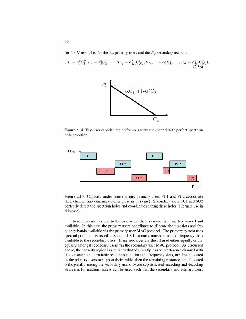
36
for the K users, i.e. for the Kp primary users and the Ks secondary users, is
(R1 = αp1C
p1 , R2 = α2
2Cp2 , . . . , RKp
= αpKp
CpKp
, RKp+1 = αs1C
s1 , . . . , RK = αs
KsCs
Ks).
(2.56)
Figure 2.14: Two-user capacity region for an interweave channel with perfect spectrum
hole detection.
Figure 2.15: Capacity under time-sharing: primary users PU1 and PU2 coordinate
their channel time-sharing (alternate use in this case). Secondary users SU1 and SU2
perfectly detect the spectrum holes and coordinate sharing these holes (alternate use in
this case).
These ideas also extend to the case when there is more than one frequency band
available. In this case the primary users coordinate to allocate the timeslots and fre-
quency bands available via the primary user MAC protocol. The primary system uses
spectral pooling, discussed in Section 1.8.1, to make unused time and frequency slots
available to the secondary users. These resources are then shared either equally or un-
equally amongst secondary users via the secondary user MAC protocol. As discussed
above, the capacity region is similar to that of a multiple user interference channel with
the constraint that available resources (i.e. time and frequency slots) are first allocated
to the primary users to support their traffic, then the remaining resources are allocated
orthogonally among the secondary users. More sophisticated encoding and decoding
strategies for medium access can be used such that the secondary and primary users

2.6. INTERWEAVE COGNITIVE RADIO NETWORKS 37
simultaneously transmit over the same channel, with rate splitting, superposition en-
coding, error-correction coding, and joint detection techniques used to ensure reliable
data detection from all users. The capacity in this case is treated based on the more
general capacity analysis of the unconstrained interference channel discussed previ-
ously in Chapter 2.4. These ideas can also be extended to the case where the secondary
transmitters are part of a broadcast or multiple access channel within the cognitive
network. Then, as before, available resources are first allocated to the primary users
to support their traffic, e.g. over a time fraction α, then the remaining resources are
allocated among the secondary users. If a secondary user is transmitting to multiple
receivers over a time fraction 1 − α, then its capacity over that time fraction will be
the corresponding broadcast capacity region instead of a single rate. Similarly, if there
are multiple secondary users transmitting to one receiver over a time fraction 1 − α,
then capacity over that time fraction will be the corresponding multiple access channel
capacity region.
The capacity results discussed above all assume perfect detection of spectrum holes
by the secondary users. There are two types of imperfect detection: missed detection
and false alarm, which are defined formally in Section 4.3. A false alarm occurs when
a primary user is detected but in fact none is present, i.e. a spectrum hole is undetected
by the secondary user or users. For a single secondary user, assuming a stationary and
ergodic system, a false alarm has no effect on the primary users (since no interference
is generated). However, it reduces the secondary user’s data rate by a fraction (1 −PFA) for PFA the probability of false alarm since, under perfect detection, the missed
spectrum holes would have been used for the secondary user’s transmission. When
there are multiple secondary users, the reduction in each of their data rates due to
false alarm depends on how the spectrum holes are allocated. If the spectrum holes
have the same length and are equally allocated among Ks secondary users, then each
of the secondary user’s data rates due to false alarm would be reduced by a fraction
(1 − PFA)/Kc.
In the case of missed detection, the secondary users fail to detect primary user ac-
tivity when in fact these users are active, i.e. a spectrum hole is detected incorrectly.
During missed detection, the channel becomes the interference channel of Fig. 2.7,
since both primary and secondary users are transmitting simultaneously. However,
in the interweave scenario, the encoding and decoding for both the primary and the
secondary users do not take this interference into account since it occurs due to an un-
expected detection error. Hence, interference from the secondary user to the primary
user will degrade its capacity. The capacity reduction is typically derived by treating
the interference as noise and computing capacity based on the SINR associated with
the interference generated by the secondary users at the primary users’ receivers. Sim-
ilarly, a secondary user transmitting during a spectrum hole obtained through missed
detection experiences interference from the primary users also occupying that hole, and
its capacity degradation can be determined in a similar manner by treating the interfer-
ence from all primary users operating during that spectrum hole as noise. Alternatively,
data transmitted when secondary and primary transmissions overlap can be declared as
erasures at the secondary receiver, assuming the receiver detects the interference and
hence doesn’t attempt to decode the data. Erasures correspond to data that cannot be
decoded except through channel codes that are designed to correct for erasures. An

38
overview of erasure-codes for cognitive radio systems can be found in [55, 81]. Pri-
mary users can also treat data received while experiencing interference from secondary
users as an erasure, but since the secondary user is typically at a much lower power
than the primary user, this is rarely done in practice; instead the interference caused by
secondary user transmissions is typically treated as noise. Since detection of spectrum
holes is a dynamic and imperfect process, the impact of false alarm or missed detec-
tion on the capacity of both primary and secondary users is characterized by ergodic or
outage capacity, as discussed in the next subsection.
A model for the impact of false alarm and missed detection on the capacity of an
interweave channel using cooperative detection between the secondary transmitter and
receiver is developed in [45]. The distributed nature of this spectrum sensing is cap-
tured mathematically via a two-switch model, one switch at the secondary transmitter
and one at the secondary receiver. When the secondary transmitter detects a spectrum
hole then it moves its switch to the ON position, and similarly at the receiver. When
both switches are ON, a hole is deemed to be present for utilization by the secondary
user, and this information is disseminated to the secondary transmitter and receiver
(perhaps via a separate cooperation channel). This model captures the fact that the far-
ther apart the secondary transmitter and receiver, the less correlated the primary user
activity will be that they each detect. Since the location of the primary receiver is un-
known, detection of primary signals at more than one location via cooperative sensing
will lead to more accurate estimation of spectrum holes, as discussed in more detail
in Chapter 5.2.1. More general models for false alarm and missed detection can be
mapped to this two-switch model via the switch probabilities of being ON or OFF. In-
ner and outer bounds on capacity of this two-switch model are developed in [45] based
on information-theoretic results for the capacity of memoryless channels with causal
and noncausal partial channel knowledge.
2.6.2 Ergodic and Outage Capacity
Ergodic and outage capacity of interweave channels capture the impact of primary
user activity and its detection on capacity. In particular, primary users may choose
to transmit or not. When they transmit, their activity can be detected correctly as
the lack of a spectrum hole, or not; when they don’t transmit, their lack of activity
can be detected correctly as a spectrum hole, or not. For a single secondary user and
assuming perfect detection of spectrum holes, we can model the interweave channel
for the secondary user as a channel with a random switch, as shown in Fig. 2.16. When
primary user activity is detected, the switch is OFF and the channel is unavailable.
When no primary activity is detected, the switch is ON, indicating that the channel
is available for the secondary user. The channel is randomly varying since within
any time interval [0, T ] the amount of time that the switch is ON or OFF, Toff and
Ton, respectively, is random. Assume that when the switch is ON, the capacity of
the channel is C , e.g. for an AWGN channel C = W log2(1 + snr) bps where Wis the channel bandwidth associated with the spectrum hole and snr is the ratio of
received signal-to-noise power at the secondary receiver (there is no interference from
primary users since detection is assumed to be perfect). The capacity of the randomly-
varying switch channel then depends on what is known about the switch position at the
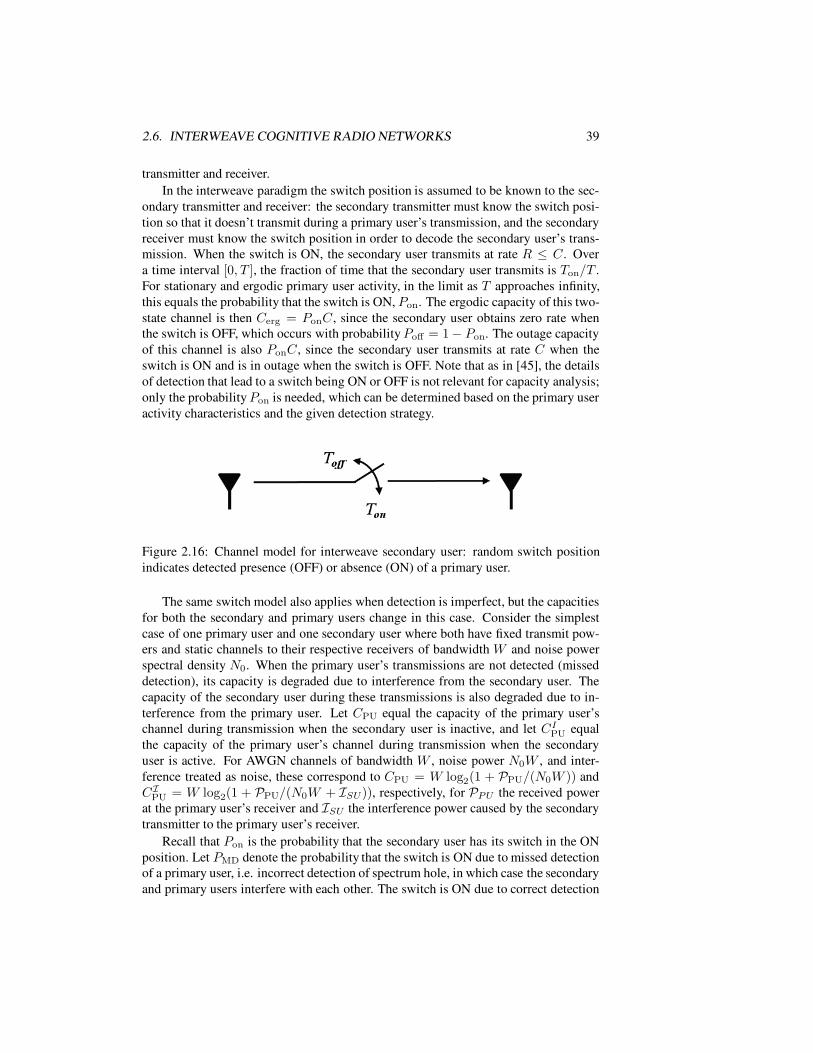
2.6. INTERWEAVE COGNITIVE RADIO NETWORKS 39
transmitter and receiver.
In the interweave paradigm the switch position is assumed to be known to the sec-
ondary transmitter and receiver: the secondary transmitter must know the switch posi-
tion so that it doesn’t transmit during a primary user’s transmission, and the secondary
receiver must know the switch position in order to decode the secondary user’s trans-
mission. When the switch is ON, the secondary user transmits at rate R ≤ C . Over
a time interval [0, T ], the fraction of time that the secondary user transmits is Ton/T .
For stationary and ergodic primary user activity, in the limit as T approaches infinity,
this equals the probability that the switch is ON, Pon. The ergodic capacity of this two-
state channel is then Cerg = PonC , since the secondary user obtains zero rate when
the switch is OFF, which occurs with probability Poff = 1− Pon. The outage capacity
of this channel is also PonC , since the secondary user transmits at rate C when the
switch is ON and is in outage when the switch is OFF. Note that as in [45], the details
of detection that lead to a switch being ON or OFF is not relevant for capacity analysis;
only the probability Pon is needed, which can be determined based on the primary user
activity characteristics and the given detection strategy.
Figure 2.16: Channel model for interweave secondary user: random switch position
indicates detected presence (OFF) or absence (ON) of a primary user.
The same switch model also applies when detection is imperfect, but the capacities
for both the secondary and primary users change in this case. Consider the simplest
case of one primary user and one secondary user where both have fixed transmit pow-
ers and static channels to their respective receivers of bandwidth W and noise power
spectral density N0. When the primary user’s transmissions are not detected (missed
detection), its capacity is degraded due to interference from the secondary user. The
capacity of the secondary user during these transmissions is also degraded due to in-
terference from the primary user. Let CPU equal the capacity of the primary user’s
channel during transmission when the secondary user is inactive, and let CIPU equal
the capacity of the primary user’s channel during transmission when the secondary
user is active. For AWGN channels of bandwidth W , noise power N0W , and inter-
ference treated as noise, these correspond to CPU = W log2(1 + PPU/(N0W )) and
CIPU = W log2(1 + PPU/(N0W + ISU)), respectively, for PPU the received power
at the primary user’s receiver and ISU the interference power caused by the secondary
transmitter to the primary user’s receiver.
Recall that Pon is the probability that the secondary user has its switch in the ON
position. Let PMD denote the probability that the switch is ON due to missed detection
of a primary user, i.e. incorrect detection of spectrum hole, in which case the secondary
and primary users interfere with each other. The switch is ON due to correct detection

40
of a spectrum hole with probability (1 − PMD) and in this case the primary user is
silent. We will first examine the impact of incorrect detection on the primary user’s
capacity. Assuming the primary user is not aware of the secondary user transmitting
due to missed detection, the correct metric for its performance while it is transmitting
is capacity versus outage. This capacity versus outage is CPU for outage probability
Pout ≥ PMDPon and CIPU for Pout < pMDPon, since the primary user can correctly
decode at transmission rate CPU unless the secondary user transmits due to missed
detection of the primary user, which occurs with probability PrmMDPon. Note that the
primary user in general does not know the secondary user’s interference, and thus it
does not know CIPU . Hence, it must choose some transmission rate R ≤ CPU without
this knowledge. If the outage probability PMDPon is acceptable, then the primary user
can transmit at rate R = CPU and accept that a fraction PMDPon of the data will be
decoded in error. If that is an unacceptable outage probability then, assuming it can
bound the maximum interference of the secondary user as ISUmax, it can transmit at a
rate R = W log2(1 +PPU/(N0W +ISUmax)). As long as the bound is accurate, data
sent at this rate will always be correctly decoded. Similarly, if it does know CIPU then
it can send at that rate with no outage.
A primary user adapting to the behavior of a secondary user is atypical for an
interweave channel, where primary users are meant to be oblivious to the presence of
secondary transmissions. However, some systems have been proposed where primary
users either aid or react to secondary users. Suppose the primary user can measure the
interference caused by the secondary user due to missed detection. Then it can adapt
its transmission rate during the time that it transmits to R = CPU in the absence of
secondary interference (i.e. when the switch is OFF) and to R = CIPU in the presence
of secondary interference (i.e. when the switch is ON due to missed detection). This
yields an ergodic rate for the primary user averaged over all time of
CergPU = PoffCPU + PMDPonC
IPU. (2.57)
since the primary user elects to be silent with probability (1 − PMD)Pon. Thus, its
ergodic rate during the time it is transmitting can be computed by dividing (2.57) by
this probability. Note that for typical wireless channels this rate can be achieved even
when the primary user’s transmitter is not adapting its rate to the presence or absence
of interference, as long as the primary user’s receiver is aware of the interference from
the secondary user [32, Chapter 4.2].
The secondary user is unaware of primary user transmissions during missed de-
tection, which happens with probability PMD. Hence the two-state switch channel of
the secondary user becomes a three-state channel: when the switch is OFF capacity
is zero since the secondary user does not transmit; when the switch is ON the ca-
pacity of the channel equals the interference-free capacity when the spectrum hole is
correctly detected, and it equals capacity with the interference from the primary user
when the hole is falsely detected. Let us consider the capacity of the channel when
the switch is in the ON position - this is a two-state channel that depends on whether
the spectrum hole is correctly detected or not. Let CSU equal the capacity of the sec-
ondary user’s channel during transmission when the primary user is inactive (correct
detection), and let CISU equal the capacity of the secondary user’s channel during trans-

2.6. INTERWEAVE COGNITIVE RADIO NETWORKS 41
mission when the primary user is active (false detection). For AWGN channels with
bandwidth W , noise power N0W and interference treated as noise, these correspond
to CSU = W log2(1 +PSU/(N0W )) and CISU = W log2(1 +PSU/(N0W + IPU )),
respectively, for PSU the received signal power at the secondary user’s receiver, and
IPMR the interference caused by the primary transmitter to the secondary user’s re-
ceiver. The correct metric for capacity of the secondary user when its channel switch
is ON is capacity versus outage. Its capacity versus outage is CSU for outage proba-
bilities Pout ≥ PMD and CISU for Pout < PMD. Similar to the case of the primary
user under missed detection above, if the outage probability PMD is acceptable, then
the secondary user can transmit at rate R = CSU and accept that a fraction PMD of
the data will be decoded in error. If that is an unacceptable outage probability then, as-
suming it can bound the maximum interference power of the primary user as IPUmax,
it can transmit at a rate R = W log2(1 + PSU/(N0W + IPUmax)) such that, as long
as the bound is accurate, data sent at this rate will be correctly decoded. Similarly, if it
does know CISU then it can send at that rate with no outage.
In addition to incorrectly detecting a spectrum hole, the secondary user may detect
the presence of a primary user when none is present, and hence turn its switch OFF
when in fact it should be ON. Given this false alarm occurs with probability PFA, the
capacity of the secondary user is reduced by PFACSU relative to the case of no false
alarm (i.e. PFA = 0), as the secondary user could transmit at rate CSU during the
missed detection periods since there is no interference from the primary user during
those periods. As with the case of perfect detection, the exact detection strategy is
not needed for capacity calculations. Only the probability of missed detection and
false alarm is used in capacity calculations, and this can be determined for any given
detection strategy, as discussed in Chapters 4 and 5.
2.6.3 Scaling Laws for Interweave Networks
In Chapter 2.3.3 we discussed scaling laws for K-user wireless networks. We now
discuss scaling laws in interweave networks with one or more primary and secondary
users. Not much is known about scaling laws for this type of network, although scaling
laws have been derived for a single-hop interweave network where multiple secondary
users transmit in the presence of a single primary user in [93]. This work defined the
notion of a primary exclusive region, or PER, around the primary transmitter. Sec-
ondary transmitters cannot operate within this PER, and the distance between a sec-
ondary user’s transmitter and receiver must be less than some specified distance. These
two constraints restrict the amount of interference a secondary transmitter can cause
to the primary receiver, and hence its outage probability, thereby enabling a closed-
form derivation of scaling laws. The capacity was found to scale linearly with the
number of secondary users, in contrast to the classical sublinear scaling in Gupta and
Kumer’s result, where multihop routing was assumed. These interweave scaling law
results were extended in [46] to a network with multiple primary as well as multiple
secondary users, along with multihop routing. This work assumes that the locations of
the primary user transmitters and receivers are known by the secondary network, and
also that the primary network is less dense than the secondary network. The multihop
routing protocols assume a preservation region around each primary node such that

42
the secondary users route their traffic around these regions. This routing protocol is
shown to achieve almost the same scaling law as if the primary network was absent,
while the primary network throughput is subject to only a fractional loss that decreases
asymptotically. Specifically, a Kp-user primary network achieves a throughput scaling
of√
Kp = K.5p while a Ks-user cognitive network achieves a throughput scaling of
K.5−δs for any δ > 0 with an arbitrarily small probability of outage. Similar scaling
laws under the same model, constraints, and assumptions were obtained in [100], how-
ever in this work the location of the primary receivers was unknown. Hence preserva-
tion regions were only formed around the primary transmitters. This paper also showed
that the same throughput-delay tradeoff as was obtained in [22] for a single asymptot-
ically large network can be achieved by both the primary and secondary networks as
the number of each type of user grows asymptotically. These results assume that the
relative density of the primary users relative to the secondary users remains the same
as the number of users grows.
2.7 Overlay Cognitive Radio Networks
The motivation for overlay cognitive radio networks is to exploit intelligent radio capa-
bilities to their fullest: 1) from the information-theoretic point of view, the interweave
constraint of orthogonal transmissions used by secondary and primary communicating
pairs is unnecessarily restrictive and, as such, reduces capacity; 2) cognitive capabili-
ties can be exploited more broadly than just for spectrum hole detection.
For these reasons, and in contrast to interweave networks, overlay cognitive ra-
dio networks allow for concurrent secondary and primary transmissions over the same
dimensions. Furthermore, in contrast to both interweave and underlay networks, in
overlay networks a secondary transmitter may improve the communication of a pri-
mary user. In this setting, relaying and techniques for coping with interference become
key tools to maximize the performance of both primary and secondary users.
Modeling Cognition
In the analysis of overlay cognitive radio models, the cognitive capability is typ-
ically captured by assuming that the secondary user’s encoder, called the cognitive
encoder, knows the data sequence to be sent by the primary encoder in the next trans-
mission block. This assumption is often too idealistic for practical systems. However,
it is reasonable when the secondary and primary transmitters are close to each other,
or the primary data sequence is being retransmitted after an initial failure and the sec-
ondary decoder was able to successfully decode it in the first transmission. This as-
sumption is also applicable when the primary transmitter sends its data sequence in
advance to a secondary transmitter, which might be done in a separate frequency band.
Although idealistic, once the encoding and decoding strategies for this channel model
under this assumption are fully understood, this assumption can be relaxed to assume:
1) that primary data sequences are conveyed to the secondary user over links of finite
capacity; 2) partial data sequence knowledge or, 3) causality in learning the primary
data sequence. These relaxations were respectively investigated in [60, 59, 9].

2.7. OVERLAY COGNITIVE RADIO NETWORKS 43
Figure 2.17: Two-user overlay channel
2.7.1 Cognitive Encoder for the Two-user Overlay Channel
The simplest overlay cognitive network consists of one secondary and one primary
pair, as shown in Fig. 2.17. The cognitive encoder corresponding to the secondary
user is assumed to have full knowledge of data sequence WP communicated by pri-
mary encoder to the primary decoder. The encoding strategies and channel gains are
assumed known to all users in the channel. Overlay encoding techniques have mostly
been investigated for this two-user channel. Without cognition, this network reduces
to the two-user interference channel of Fig. 2.11 the secondary user corresponding to
User 1 and the primary user corresponding to User 2. Due to the similarities between
these two models, in the information theory literature, this network is referred to as the
interference channel with one cognitive encoder. It is also referred to as the cognitive
radio channel, the interference channel with asymmetric message knowledge, the in-
terference channel with degraded message sets or the cognitive interference channel.
Another special case of this channel model is obtained when the primary user does not
transmit. Since the secondary transmitter knows the messages intended for both re-
ceivers, the channel reduces to the broadcast channel [16]. The two-user overlay chan-
nel thus contains elements of both interference and broadcast channels. The encoding
strategies that have been developed for these canonical channels, or their combinations,
are capacity-achieving for the overlay channel in certain conditions. We next review
the encoding strategies that have been proposed for the two-user overlay channel, and
discuss scenarios in which these schemes or their combinations achieve capacity.
Formally, the two-user overlay channel, with one secondary (cognitive) user and
one primary user consists of two input alphabets XS ,XP , two output alphabets YS ,YP ,
and a conditional probability distribution p(ys, yp|xs, xp), where (xs, xp) ∈ Xs × Xp
are channel inputs and (ys, yp) ∈ Y1×Y2 are channel outputs. The secondary source ss
wishes to send a message Ws ∈ W = {1, . . . , 2nRs} to its destination, and the primary
source sp wishes to send a message Wp ∈ W = {1, . . . , 2nRp} to its destination. Data
sequence Wp is also known at the secondary (cognitive) encoder. An (Rs, Rp, n) code
consists of two data sequence sets Ws,Wp, encoding functions
Xns = fs(Ws, Wp) (2.58)
Xnp = fp(Wp) (2.59)

44
and two decoding functions
Ws = gs(Yns ), Wp = gp(Y
np ). (2.60)
The error probability of the code is
Pe = P[[
Ws 6= Ws
]
⋃
[
Wp 6= Wp
]]
. (2.61)
A rate pair (Rs, Rp) is achievable if, for any ε > 0, there exists, for sufficiently large
n, an (Rs, Rp, n) code such that Pe ≤ ε. The capacity region of the two-user overlay
channel is the closure of the set of all achievable rate pairs (Rs, Rp).
We observe that the only difference between this definition and the corresponding
definitions for the interference channel is in the encoding function of the secondary
cognitive encoder (2.58). Unlike in the interference channel, in this case the encoder
knows both data sequences Ws and Wp and can thus form encoded sequences that
depend on both of them. We will also consider the AWGN interference channel given
by (2.29), augmented with cognitive encoding by the secondary user.
The additional information allows the cognitive encoder to deploy cooperation to
increase the rate of the primary pair and precoding against interference to increase its
own rate. Before summarizing encoding strategies used by the cognitive encoder, we
give a brief overview of the Gelfand-Pinsker encoding technique. This technique, also
referred to as binning, is used for the precoding against interference.
Gelfand-Pinsker Coding
For overlay networks, transmission by any primary transmitter causes interference
at the secondary receiver. Since the cognitive encoder knows this interference, it de-
ploys an encoding scheme that mitigates the effect of the interference at its receiver,
thereby increasing its rate. In the overlay channel, since the cognitive encoder has per-
fect knowledge of the data sequence and the encoding strategy of the primary user, the
secondary transmit-receiver pair can view this situation as communication in a channel
with a random state noncausally known at the encoder, also known as the Gelfand-
Pinsker problem [30], shown in Fig. 2.18. In this figure, a single source communicates
data sequence W ∈ {1, . . . , 2nR} to the destination over a channel given by p(y|x, s).The channel state sequence Sn is assumed to be a random i.i.d. sequence generated
from the distribution p(s) over the random state. Sn is noncausally known at the en-
coder.
We next consider an AWGN channel where the random state is an additional in-
terference term S. Specifically, an AWGN channel with a random interference state is
given by
Y = X + S + Z (2.62)
where Z is zero-mean Gaussian noise at the receiver with power N and S is zero-
mean Gaussian noise at the receiver with power Ns. The transmit power constraint
is E[X2] ≤ P. The Gelfand-Pinsker encoding in this channel model reduces to DPC,
described above for the interference channel, whereby precoding is used to cancel the
effect of the inteference term S. In this setting DPC achieves the capacity of the AWGN

2.7. OVERLAY COGNITIVE RADIO NETWORKS 45
Figure 2.18: A channel with a random state. The state Sn is known noncausally at the
encoder.
channel as if there were no interference, i.e. it completely cancels the effect of inter-
ference S, yielding capacity
C = W log2
(
1 +PN
)
. (2.63)
The capacity of the general discrete-time memoryless channel with random state is
given by
C = maxp(u|s),f(·)
I(U ; Y ) − I(U ; S) (2.64)
where U − (X, S) − Y form a Markov chain, and is achieved by Gelfand-Pinsker
encoding [30]. The role of the random variable U is to generate a codebook at the
encoder that will allow, in each transmission, a codeword that depends both on the data
sequence and on the random state Sn . The Gelfand-Pinsker encoding can play a crucial
role in overlay cognitive radio, as will be described next.
Communication schemes deployed in the overlay channel contain the following
three encoding strategies:
1. Rate-splitting; Rate-splitting, as briefly described in Section 2.4, can improve
rates for both communicating pairs by enabling (partial) interference cancellation
at the decoders in the same fashion as in interference channels without cognition.
This technique can potentially be deployed by both encoders, as it requires no
cognition about other user’s data sequences as the encoder is only splitting its
own rate. For the rate-splitting to be exploited by the primary user, this ap-
proach requires that the decoding at the primary receiver be modified to decode
and cancel part of secondary user’s transmission. This approach differs from the
approach used in interweave and underlay cognitive radio where the communi-
cation technique of the primary users is not adapted in the presence of secondary
users. If this constraint were to be imposed in overlay cognitive networks as
well, the rate-splitting is no longer applicable since it requires that the primary
receiver decodes a part of the message of the secondary user.
2. Cooperation; Full, partial or delayed knowledge of the primary user’s data se-
quence allows the cognitive encoder to relay this information to the primary user,

46
thereby increasing the rate of the primary pair. The cognitive encoder uses a frac-
tion of its power to transmit message Wp to the primary user and thus increase the
primary rate Rp. When the primary user’s data sequence (or a part of it) is known
to the cognitive encoder without the delay, i.e., at the beginning of the transmis-
sion block, relaying is performed via superposition coding, where secondary and
primary messages are superimposed and sent by the cognitive encoder. Due to
the noncausal knowledge, there is no need for Markov block encoding otherwise
used for relaying [17].
3. Gelfand-Pinsker Encoding (Binning); Any signal carrying all or part of Wp is
interference at the secondary receiver. Hence, both the primary encoder as well
as the cognitive encoder cause interference at the secondary receiver. However,
if the cognitive encoder knows Wp at the beginning of the transmission block
(as well as the codebooks and channel state information), it can infer the inter-
ference created at the secondary receiver. Knowing the interference, it can apply
Gelfand-Pinsker encoding and, specifically in AWGN channels, DPC in order to
pre-cancel this interference. Another motivation for deploying Gelfand-Pinsker
encoding is found in the relationship between the overlay channel and the broad-
cast channel whereby when the primary transmitter is silent, the overlay chan-
nel reduces to a two-user broadcast channel. For the discrete-time memoryless
broadcast channel, the encoding scheme that yields the largest known achiev-
able rate region is based on Gelfand-Pinsker encoding [61]. In the Gaussian case
the two-user overlay channel is related also to the MIMO Gaussian broadcast
channel. Specifically, a MIMO broadcast channel with two transmit antennas is
equivalent to a two-user overlay channel when both encoders are cognitive, i.e.
both encoders know the message intended for each receiver, since in fact these
encoders are part of the same broadcasting transmission strategy. For MIMO
Gaussian broadcast channels, DPC is the optimal encoding strategy [94, 92].
Motivated by these observations, binning and DPC have been applied to the two-
user overlay channel, resulting in the highest known achievable rates, including
capacity, in some cases, as will be presented later in this section.
2.7.2 Capacity Results
Determining the capacity region for the general overlay channel remains an open prob-
lem. However, as for the interference channel without cognition, the capacity has been
determined for some regimes. The capacity in strong interference has been determined
in [60, Thm. 5]. The capacity for the Gaussian channel in weak interference has been
derived in [95], [49]. For a more general case that unifies the results under these two
regimes, the capacity was determined in [70]. For a class of discrete memoryless cog-
nitive Z-channels (i.e., channels where there is no interference at the primary receiver)
in which only the receiver of the secondary pair suffers interference the capacity has
been determined in [57]. Capacity of a class of Gaussian cognitive Z-channels for the
opposite case, when the interference is at the primary receiver, has been found in [47].
In each case, some combination of rate-splitting, cooperation and/or binning achieves
capacity. These regimes and their capacity-achieving encoding techniques are as fol-

2.7. OVERLAY COGNITIVE RADIO NETWORKS 47
lows:
1. Strong interference [60]. As in the interference channel, this is the regime in
which both decoders can decode each other’s messages without rate penalty. In
AWGN interference channels with one cognitive encoder (2.29), the following
interference conditions are sufficient for strong interference to be satisfied:
|b| ≥ 1
|a| ≥ b
α+
|α− 1|α
if ab > 0
|a| ≥ b
α+
α + 1
αif ab < 0 (2.65)
where α =√
Ps/Pp,
with Ps is the power associated with the secondary user and Pp is the power
associated with the primary user. For PS = PP and a, b ≥ 0 these conditions
simplify to
b ≥ 1, a ≥ b. (2.66)
In a general discrete-time memoryless channel, these conditions can be expressed
in terms of the conditional mutual information as
I(Xs; Ys|Xp) ≤ I(Xs; Yp|Xp)
I(Xs, Xp; Ys) ≤ I(Xs, Xp; Yp), (2.67)
and need to be satisfied for all input distributions p(xs, xp). We observe that
the first inequality is the same as in the interference channel. In this regime,
cooperation via superposition coding achieves capacity. The capacity region in
AWGN channel is given by:
C =⋃
|ρ|≤1
{
(Rs, Rp) : Rs ≥ 0, Rp ≥ 0,
Rs ≤1
2log(
1 + (1 − ρ2)Ps
)
(2.68)
Rs + Rp ≤ 1
2log(
1 + Ps + Pp + b2Ps + 2ρb√
PsPp
)}
, (2.69)
where ρ is the correlation between inputs Xs and Xp. Note that a larger ρ results
in a larger coherent combining gain. The general capacity region is given by:
C =⋃
{
(Rs, Rp) : Rs ≥ 0, Rp ≥ 0,
Rs ≤ I(Xs; Ys|Xp) (2.70)
Rs + Rp ≤ I(Xs, Xp; Yp)}
, (2.71)
where the union is over all input distributions p(xs, xp).

48
2. Weak interference at the primary receiver [95], [49].
In the AWGN overlay channel (2.29), weak interference at the primary receiver
corresponds to |b| ≤ 1, i.e., the cross-channel gain from the secondary to the pri-
mary user is smaller than the direct link gain. Because the interference is weak,
the primary receiver does not attempt to decode the unwanted data sequence and
instead treats it as noise. Interference at the secondary receiver can be eliminated
by DPC at the cognitive encoder, allowing for the interference-free, single-user
rate to be achieved. The optimum coding strategy at the cognitive encoder con-
sists of encoding message W1 via DPC while treating the primary user’s input
sequence Xn2 as interference, and superposition coding to help convey W2 to the
primary receiver. Thus, there is no need for rate-splitting; DPC and cooperation
via superposition coding achieve capacity. The capacity region is given by:
Rs ≤ 1
2log(1 + (1 − α)Ps) (2.72)
Rp ≤ 1
2log
(
1 +(b√
αPs +√
Pp)2
1 + b2(1 − α)Ps
)
, (2.73)
where α is the fraction of power that the cognitive encoder uses for cooperation.
The rest of the power, (1−α)Ps, the encoder uses to transmit signal carrying its
own data. That signal is the interference at the primary receiver.
In the case of the discrete-time memoryless channel, the weak interference con-
ditions are given by:
I(U ; Yp|Xp) ≤ I(U ; Ys|Xp)
I(Xp; Yp) ≤ I(Xp ; Ys) (2.74)
for all distributions p(u, xs, xp). The random variable U has the same role as
in the Gelfand-Pinsker encoding, i.e., it is used for precanceling the interference
via binning. The capacity region is given by
C =⋃
{
(Rs, Rp) : Rs ≥ 0, Rp ≥ 0,
Rs ≤ I(Xs; Ys|U, Xp) (2.75)
Rp ≤ I(U, Xp; Yp)}
(2.76)
where the union is over all distributions p(u, xs, xp).
Regimes of strong and weak interference for Gaussian channels with Ps = Pp
for a, b ≥ 0 are shown in Fig. 2.19.
3. Better cognitive decoding regime [70].
This is the regime for which the condition
I(U, Xp; Yp) ≤ I(U, Xp; Ys) (2.77)
holds for any p(u, xs, xp).
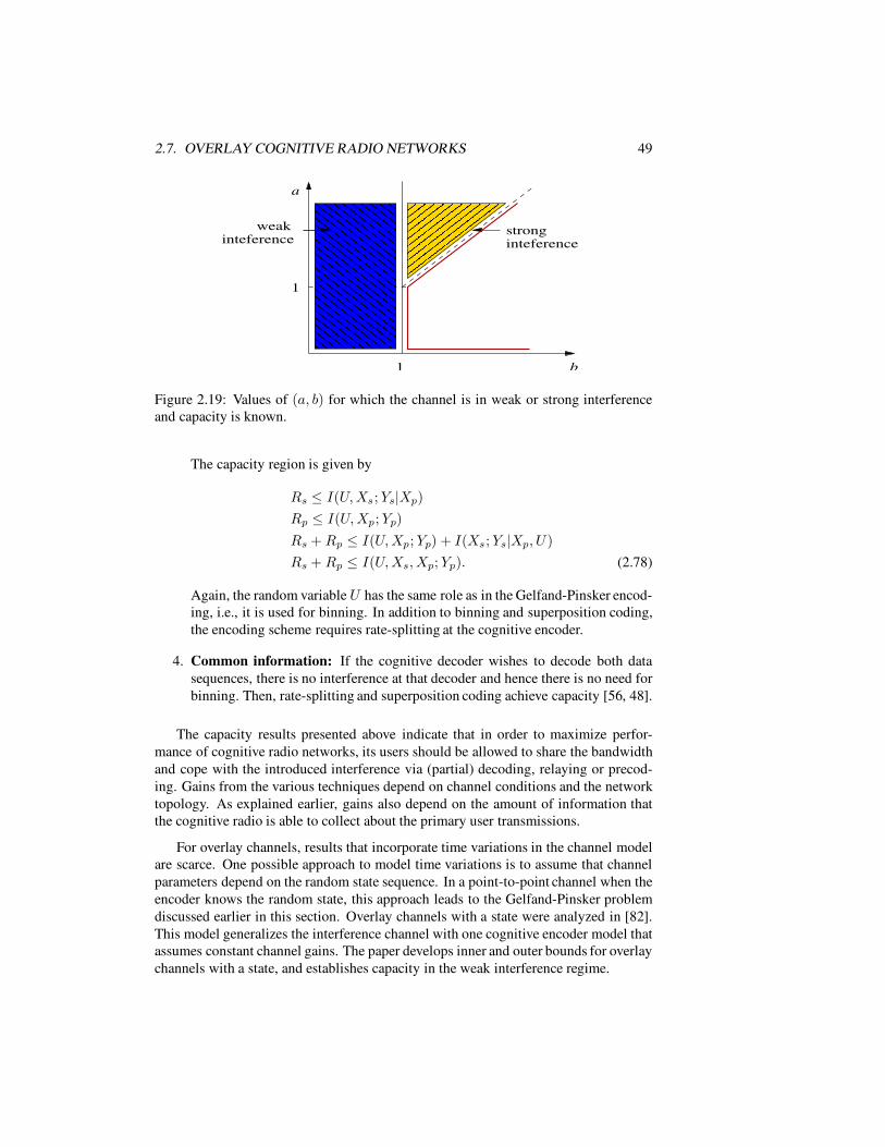
2.7. OVERLAY COGNITIVE RADIO NETWORKS 49
inteference
� � � � � �� � � � � �� � � � � �� � � � � �� � � � � �� � � � � �
� � � � � �� � � � � �� � � � � �� � � � � �� � � � � �� � � � � �
� � � � �� � � � �� � � � �� � � � �� � � � �� � � � �� � � � �� � � � �� � � � �� � � � �� � � � �
� � � � �� � � � �� � � � �� � � � �� � � � �� � � � �� � � � �� � � � �� � � � �� � � � �� � � � �
1
b
a
1
stronginteference
weak
Figure 2.19: Values of (a, b) for which the channel is in weak or strong interference
and capacity is known.
The capacity region is given by
Rs ≤ I(U, Xs; Ys|Xp)
Rp ≤ I(U, Xp; Yp)
Rs + Rp ≤ I(U, Xp; Yp) + I(Xs; Ys|Xp, U)
Rs + Rp ≤ I(U, Xs, Xp; Yp). (2.78)
Again, the random variable U has the same role as in the Gelfand-Pinsker encod-
ing, i.e., it is used for binning. In addition to binning and superposition coding,
the encoding scheme requires rate-splitting at the cognitive encoder.
4. Common information: If the cognitive decoder wishes to decode both data
sequences, there is no interference at that decoder and hence there is no need for
binning. Then, rate-splitting and superposition coding achieve capacity [56, 48].
The capacity results presented above indicate that in order to maximize perfor-
mance of cognitive radio networks, its users should be allowed to share the bandwidth
and cope with the introduced interference via (partial) decoding, relaying or precod-
ing. Gains from the various techniques depend on channel conditions and the network
topology. As explained earlier, gains also depend on the amount of information that
the cognitive radio is able to collect about the primary user transmissions.
For overlay channels, results that incorporate time variations in the channel model
are scarce. One possible approach to model time variations is to assume that channel
parameters depend on the random state sequence. In a point-to-point channel when the
encoder knows the random state, this approach leads to the Gelfand-Pinsker problem
discussed earlier in this section. Overlay channels with a state were analyzed in [82].
This model generalizes the interference channel with one cognitive encoder model that
assumes constant channel gains. The paper develops inner and outer bounds for overlay
channels with a state, and establishes capacity in the weak interference regime.

50
Another important aspect of this problem is the impact of imperfect channel state
information (CSI) at the cognitive encoder. The lack of channel knowledge will affect
all cognitive encoding schemes. With phase uncertainty at the cognitive encoder, DPC
cannot be applied directly. Hence this uncertainty precludes canceling interference and
results in significant performance loss [37]. In this case, feedback about channel state
information to the cognitive encoders could be very beneficial. Relaying strategies can
be realized without CSI at the transmitter, but would require CSI at the receiver [52].
However, CSI at the transmitter could allow for additional relaying approaches (e.g.,
beamforming) and thus further improve the network performance.
2.7.3 K-user Overlay Networks
Analysis of the two-user overlay channel focuses on a single secondary pair and a sin-
gle primary pair. Yet, as in the interweave networks, multiple secondary and multiple
primary users in the overlay network can simultaneously share the same spectrum. As
with the two-user overlay case, in this more general setting we also seek efficient ways
to minimize interference among users.
We have seen in Section 2.4 that for the K-user interference channel, generalizing
the rate-splitting approach as a way to cope with interference from multiple senders is
too complex. Moreover, this approach can be outperformed by collective treatment of
interference via interference alignment or structured codes. Not surprisingly, interfer-
ence alignment as well as structured codes are promising approaches for the K-user
overlay cognitive radio network as well. These techniques could be deployed by cog-
nitive nodes to reduce the interference at both the primary and the cognitive receivers.
But in contrast to the encoders in interference channels, secondary users can also per-
form relaying of primary messages, and precoding against interference. The interplay
between these techniques is not yet well understood and presents an important and
interesting research topic.
Another interesting problem is the impact of cognition when present at different
points in the network. In particular, not only encoders but also (or only) decoders
can be cognitive. This will significantly impact the available encoding and decoding
techniques. No cognition at the encoder will preclude both cooperation and precoding
techniques. On the other hand, it will enable decoders to directly cancel interference.
The impact of different points of cognition in the case of single primary and secondary
pair has been investigated in [44].
Once the capacity results and achievable rates, along with their encoding and de-
coding strategies, are obtained indicating the most promising encoding approaches,
protocols for coexistence among many secondary users will need to be developed. As
a final remark we note that in principle the presence of cognitive radios in overlay sys-
tems can improve not only spectrum utilization and rates of both primary and secondary
users, but also the robustness, the delay and the energy consumption of the primary sys-
tem. The presence of cognitive transmitters that have the ability to learn primary users’
information enables this information to be send over multiple paths in the network,
thereby adding diversity to the primary system, and deploying more energy and delay
efficient paths for information flow in the network. However, the implementation chal-
lenges associated with overlay systems may preclude many of these potential benefits

2.8. SUMMARY 51
being realized in practice.
2.8 Summary
Determining the fundamental performance limits of general cognitive radio networks is
a daunting challenge. Few fundamental performance bounds are available for conven-
tional wireless networks, let alone when a second tier of cognitive users is introduced
into such a network. The most common metric for performance of wireless systems
is Shannon capacity. Although there are few capacity results for general wireless net-
works, this chapter has described how existing Shannon-theoretic tools can be used
directly or extended to obtain some results or bounds on the fundamental capacity lim-
its of cognitive networks.
The building block for all known cognitive network capacity results is the two-
user interference channel, where one primary transmit-receiver pair and one secondary
transmit-receive pair share a common channel. This simple four-node network mod-
els all three cognitive radio paradigms — underlay, interweave, and overlay — with
one secondary user and one primary user. Specifically, in the underlay paradigm the
cognitive transmitter is restricted such that its interference to the primary receiver is
below some threshold, in the interweave paradigm the cognitive transmitter may only
transmit when it detects a spectrum hole, and in the overlay paradigm both users trans-
mit simultaneously, with the secondary user improving the performance of the primary
user while obtaining some bandwidth for its own communication. Based on this four-
node model, we have shown that the capacity region of an underlay network can be
determined based on Shannon capacity analysis with the interference from the primary
users to the secondary users, and the interference from the secondarye users to the
primary users, treated as AWGN. Hence, capacity of an underlay single-user channel,
with fading and multiple antennas, as well as that of a multiple access and broadcast
underlay channel, is the same as in the absence of primary users, except that the trans-
mit power of the secondary user(s) is constrained relative to the interference caused to
the primary users. In this case of multiple secondary users, a MAC protocol may also
be used when the sum of secondary interference exceeds the primary users’ threshold,
so that some of the secondary users stop transmitting to reduce the total interference
below the required level.
Treating interference as noise is also used in the capacity analysis of interweave
networks. However, unlike in underlay networks, interweave capacity analysis requires
that the dynamics associated with detection of primary user activity, as well as the prob-
ability of missed detection and false alarm, be incorporated into the capacity analysis.
To capture these dynamics, the secondary user’s interweave channel in the four-node
case is modeled as a switch. When the switch is ON, the secondary user has detected
a spectrum hole (lack of primary user activity) and transmits. When the switch is
OFF, the secondary transmitter is silent, and the primary user experiences no interfer-
ence. If a spectrum hole is correctly detected, then the secondary user experiences no
interference; when the spectrum hole is incorrectly detected, both the secondary and
primary users transmit simultaneously and interfere with each other’s transmissions.
Given the time variations of the switch, under perfect detection the secondary user’s
52
channel can be modeled as a two-state channel corresponding to the switch being ON
or OFF. Using this model, the ergodic and outage capacities are derived. Under im-
perfect detection both the primary and secondary user channels have three states. For
the secondary user’s channel, the switch can be OFF or ON; when the switch is OFF
there is no transmission, when the switch is ON, the spectrum hole can be correctly
(resulting in no interference) or incorrectly (primary user interference) detected. Since
the secondary user is not aware of false detections, the correct capacity metric is capac-
ity versus outage, which can be computed based on the probability of missed detection
and the SINR that results due to primary user interference. Similarly, the primary user
experiences interference from the secondary user due to missed detection, and its ca-
pacity versus outage can be computed based on this missed detection probability and
the SINR resulting from secondary user interference. These capacity calculations can
be generalized to multiple primary and secondary users by generalizing the models for
missed detection and false alarm along with the resulting interference.
Overlay networks do not treat interference as noise. Instead novel encoding and
decoding strategies are used by the secondary users to enhance the performance of the
primary users while obtaining some interference-free bandwidth for their own trans-
missions. These encoding techniques include rate splitting, whereby one user splits
its data sequence and encodes it via superposition coding such that a part of this se-
quence can be decoded and removed by the receiver of the other user. In the overlay
network, this would allow the secondary transmitter’s interference to be removed by
the primary receiver. However, this interference removal requires a modified decoder
for the primary user, so it is not applicable when the primary system is oblivious to
the secondary system in terms of its design or operation. In addition to rate splitting,
the secondary encoder uses its knowledge of the primary user’s encoded data sequence
to enhance the transmission of the sequence to the primary receiver via a cooperative
protocol. Finally, knowledge of the primary user’s data sequence allows the secondary
transmitter to employ Gelfand-Pinsker encoding, or binning, to pre-cancel the interfer-
ence that the primary user causes to the cognitive receiver. Similarly, if the primary
user knows the secondary user’s sequence, it can use binning in a similar fashion.
These information-theoretic strategies have not yet made their way into commercial
systems, where underlay and interweave currently dominate. Moreover, extensions of
these ideas to networks of more than a few secondary and primary users remain open
problems. However, as this chapter has shown, the overlay paradigm holds significant
promise for increasing the capacity of both secondary and primary users above that
of the other cognitive radio paradigms. If these information-theoretic results can be
translated to practice, then perhaps at some point in the future overlay systems will
dominate the cognitive radio landscape.
There are many open problems in determining fundamental performance limits of
cognitive networks. In the context of underlay networks, capacity when nodes have
multiple antennas that can direct secondary transmissions away from primary users has
not yet been investigated. Capacity versus outage based on incorrect information about
the interference caused between primary and secondary users has also not yet been ex-
plored. For interweave networks, there is much active research to determine optimal
medium access protocols that achieve capacity. In addition, the scaling laws to date as-
sume single-hop routing and an exclusion region around the primary users — perhaps

2.9. FURTHER READING 53
these scaling laws can be improved upon by considering relaying as well as hierarchi-
cal cooperation, which have proved fruitful in developing improved scaling laws for
noncognitive networks. Capacity results for overlay networks to date mainly assume
one secondary and one primary user. Since the capacity regions for conventional ad hoc
networks with more than a few users have proved elusive, we expect the same will be
true with overlay networks, unless somehow the intelligence associated with cognition
proves to simplify the problem and facilitate a solution. There are few fundamental
performance results for metrics other than capacity such as energy, delay, and com-
plexity, nor have asymptotic scaling laws been developed for any of these networks. In
particular, while capacity strategies for overlay networks with more than a few nodes
may be difficult to obtain, perhaps scaling laws that exploit previous work on scal-
ing in the absence of primary users can be extended to take the primary network into
account. Performance bounds with respect to energy require models for energy con-
sumption that includes both transmit and circuit (analog and processor) energy, which
have proved difficult to obtain. This complicates determining tradeoffs between per-
formance (which improves via sophisticated signal processing and encoding/decoding)
and energy consumption. Indeed, the development of fundamental performance met-
rics for cognitive networks is a rich and active area of research. Results in this area will
prove essential to obtain insights and performance bounds for these emerging systems.
The next chapter develops the models associated with signal propagation in cog-
nitive networks. These models are critical to determine the nature of interference at
primary receivers and of the desired received signals at all receivers. In particular, dif-
ferent radio bands will have very different interference characteristics since propaga-
tion is highly dependent on frequency. Moreover, the time-variations of these channels
dictate how well the information required under the different cognitive user paradigms
can be obtained, and how fast such systems need to adapt. The next chapter describes
the models for these different aspects of cognitive radio channels.
2.9 Further Reading
The four-node cognitive radio channel is a special case of the four-node interference
channel, whose capacity was first investigated in the late 1970s by Sato and by Carleial
[73, 11]. The model where one encoder in the interference channel is a cognitive
encoder was first proposed and its capacity region analyzed in [19]. Since then there
has been tremendous activity determining achievable rate regions and capacity outer
bounds for this channel, as well as special cases such as strong, very strong, and weak
interference regimes where these bounds meet. Tutorial papers [20, 35] describe the
large body of work on the capacity of interference channels with cognitive encoders
and the resulting capacity regions and encoding/decoding strategies for these special
regimes. Scaling laws for interweave networks were first investigated in [93] using the
idea of a primary exclusion region. The first work to analyze capacity of the interweave
channel based on a switch model for primary user detection was [45].

54

Bibliography
[1] V. S. Annapureddy and V. Veeravalli. Gaussian interference networks: Sum
capacity in the low interference regime and new outer bounds on the capacity
region. Submitted to the IEEE Transactions on Information Theory. Preprint at
http://arxiv.org/abs/0802.3495.
[2] M. R. Aref. Information Flow in Relay Networks. Ph.D thesis, Stanford Univ.,
Stanford, CA, 1980.
[3] Changhun Bae and W.E. Stark. End-to-end energy/bandwidth tradeoff in multi-
hop wireless networks. IEEE Transactions on Information Theory, vol. 55, no.
9, pp. 4051 –4066, September 2009.
[4] E. Biglieri, J. Proakis, and S. Shamai (Shitz). Fading channels: Information the-
oretic and communication aspects. IEEE Transactions on Information Theory,
vol. 44, no. 6, pp. 2619–2692, October 1998.
[5] H. Bolcskei, R.U. Nabar, O. Oyman, and A.J. Paulraj. Capacity scaling laws in
MIMO relay networks. IEEE Transactions on Wireless Communications, vol 5,
no. 6, pp. 1433–1444, June 2006.
[6] R. Brodersen, A. Wolisz, D. Cabric, S. M. Mishra, and D. Willkomm.
CORVUS: A cognitive radio approach for usage of virtual unlicensed spec-
trum. White Paper: Berkeley Wireless Research Center. Download available
at http://bwrc.eecs.berkeley.edu/research/mcma/CR White paper final1.pdf.
[7] V. R. Cadambe and S. A. Jafar. Interference alignment and degrees of freedom
of the K-User interference channel. IEEE Transactions on Information Theory,
vol. 54, no. 8, pp. 3425–3441, August 2008.
[8] V. R. Cadambe and S. A. Jafar. Parallel Gaussian interference channels are not
always separable. IEEE Transactions on Information Theory, vol. 55, no. 9, pp.
3983–3990, September 2009.
[9] Y. Cao and B. Chen. Interference channel with one cognitive transmitter. In
Proc. of the Asilomar Conference on Signals, Systems, and Computers, Pacific
Grove, CA, USA, October 26–29, 2008.
55

56 BIBLIOGRAPHY
[10] A. B. Carleial. A case where interference does not reduce capacity. IEEE Trans-
actions on Information Theory, vol. 21, no. 5, pp. 569–570, September 1975.
[11] A. B. Carleial. Interference channels. IEEE Transactions on Information The-
ory, vol. 24, no. 1, pp. 60–70, January 1978.
[12] T.C. Clancy. Achievable capacity under the interference temperature model.
In Proc. of the IEEE International Conference on Computer Communications
(INFOCOM) , Anchorage, AK, USA, May 6–12, 2007, pp. 794 –802.
[13] C.B. Cormio and K.R.A. Chodhury. A survey on MAC protocols for cognitive
radio networks. Elsevier Journal on Ad Hoc Networks, vol. 7, no. 7, pp. 1315–
1329, July 2009.
[14] M. Costa. Writing on dirty paper. IEEE Transactions on Information Theory,
vol. 29, no. 3, pp. 439–441, May 1983.
[15] M. H. M. Costa and A. El Gamal. The capacity region of the discrete mem-
oryless interference channel with strong interference. IEEE Transactions on
Information Theory, vol. 33, no. 5, pp. 710–711, September 1987.
[16] T. Cover. Broadcast channels. IEEE Transactions on Information Theory, vol.
18, no. 1, pp. 2–14, January 1972.
[17] T. Cover and A. El Gamal. Capacity theorems for the relay channel. IEEE
Transactions on Information Theory, vol. 25, no. 5, pp. 572–584, September
1979.
[18] T. Cover and J. Thomas. Elements of Information Theory, 2nd Ed., Wiley, 2005.
[19] N. Devroye, P. Mitran, and V. Tarokh. Achievable rates in cognitive radio chan-
nels. IEEE Transactions on Information Theory, vol. 52, no. 5, pp. 1813 – 1827,
May 2006.
[20] N. Devroye, M. Vu, and V. Tarokh. Cognitive radio networks. IEEE Signal
Processing Magazine, vol. 25, no. 6, pp. 12 –23, November 2008.
[21] M. Effros, A. Goldsmith, and Y. Liang. Generalizing capacity: New definitions
and capacity theorems for composite channels. IEEE Transactions on Informa-
tion Theory, vol. 56, no. 7, July 2010.
[22] A. El Gamal, J. Mammen, B. Prabhakar, and D. Shah. Optimal throughput-
delay scaling in wireless networks - part I: the fluid model. IEEE Transactions
on Information Theory, vol. 52, no. 6, pp. 2568 –2592, June 2006.
[23] R. Etkin, D. Tse, and H. Wang. Gaussian interference channel capacity to within
one bit. IEEE Transactions on Information Theory., vol. 54, no. 12, pp. 5534–
5562, May 2008.

BIBLIOGRAPHY 57
[24] Federal Communications Commission Spectrum Policy Task Force.
Report of the Spectrum Efficiency Working Group. Techni-
cal Report 02-135, (November), 2002. Download available at
http://www.fcc.gov/sptf/files/SEWGFinalReport 1.pdf.
[25] R.G. Gallager. Information Theory and Reliable Communication. Wiley, 1968.
[26] A. El Gamal. On information flow in relay networks. In Proc. of the IEEE
National Telecommunications Conference, vol. 2, November 1981, pp. D4.1.1-
D4.1.4.
[27] A. El Gamal and Y-H. Kim. Network Information Theory. Cambridge University
Press, 2012.
[28] H. El Gamal, G. Caire, and M. O. Damen. The MIMO ARQ channel: Diversity-
multiplexing-delay tradeoff. IEEE Transactions on Information Theory, vol. 52,
no. 8, pp. 3601-3621, August 2006.
[29] M. Gastpar. On capacity under receive and spatial spectrum-sharing constraints.
IEEE Transactions on Information Theory, vol. 53, no. 2, pp. 471–487, February
2007.
[30] S. I. Gel’fand and M. S. Pinsker. Coding for channel with random parameters.
Probl. Peredachi Informatsii, vol. 9, no. 1, pp. 19–31, January 1980.
[31] A. Ghasemi and E. Sousa. Fundamental limits of spectrum-sharing in fading
environments. IEEE Transactions on Wireless Communications, vol. 6, no. 2,
pp. 649–658, February 2007.
[32] A. J. Goldsmith. Wireless Communications. Cambridge University Press, 2005.
[33] A. J. Goldsmith, S. A. Jafar, N. Jindal and S. Vishwanath. Capacity limits of
MIMO channels. IEEE J. on Selected Areas in Commununications, vol. 21, no.
5, pp. 684 – 702, June 2003.
[34] A. Goldsmith, M. Effros, R. Koetter, M. Medard, A. Ozdaglar, and L. Zheng.
Beyond Shannon: the quest for fundamental performance limits of wireless ad
hoc networks. IEEE Communications Magazine, vol. 49, no. 5, pp. 195 –205,
May 2011.
[35] A. Goldsmith, S. Jafar, I. Maric, and S. Srinivasa. Breaking spectrum gridlock
with cognitive radios: an information theoretic perspective. Proceedings of the
IEEE, vol. 97, no. 5, pp. 894 – 914, May 2009.
[36] M. Grossglauser and D.N.C. Tse. Mobility increases the capacity of ad hoc
wireless networks. IEEE/ACM Transactions on Networking, vol. 10, no. 4, pp.
477 – 486, August 2002.

58 BIBLIOGRAPHY
[37] P. Grover and A. Sahai. What is needed to exploit knowledge of primary trans-
missions? In Proc. of the IEEE International Symposium on New Frontiers in
Dynamic Spectrum Access Networks (DySPAN), Dublin, Ireland April 17–20,
2007, pp. 462–471.
[38] P. Gupta and P.R. Kumar. The capacity of wireless networks. IEEE Transactions
on Information Theory, vol. 42, no. 2, pp. 388–404, March 2000.
[39] P. Gupta and P.R. Kumar. Towards an information theory of large networks: an
achievable rate region. IEEE Transactions on Information Theory, vol. 49, no.
8, pp. 1877 – 1894, August 2003.
[40] T. Han and K. Kobayashi. A new achievable rate region for the interference
channel. IEEE Transactions on Information Theory, vol. 27, no. 1, pp. 49–60,
January 1981.
[41] S. Haykin. Cognitive Radio: Brain-Empowered Wireless Communications.
IEEE J. Select. Areas Commun., vol. 23, no. 2, pp. 201 – 220, February 2005.
[42] W. Hirt and J.L. Massey. Capacity of the discrete-time Gaussian channel with
intersymbol interference. IEEE Transactions on Information Theory, vol. 34,
no. 3, pp. 380–388, May 1998.
[43] J. Huang, R. A. Berry and M. L. Honig. Spectrum sharing with distributed
interference compensation. In Proc. of the IEEE International Symposium on
New Frontiers in Dynamic Spectrum Access Networks (DySPAN), Baltimore,
MD, USA, November 8–11, 2005, pp. 88 – 93.
[44] S. A. Jafar and S. Shamai(Shitz). Degrees of freedom region for the MIMO X
channel. IEEE Transactions on Information Theory, vol. 54, no. 1, pp. 151–170,
January 2008.
[45] S. A. Jafar and S. Srinivasa. Capacity Limits of Cognitive Radio with Distributed
and Dynamic Spectral Activity. IEEE J. Select. Areas Commun., vol. 25, no. 3,
pp. 529–537, April 2007.
[46] S.-W. Jeon, N. Devroye, M. Vu, S.-Y. Chung, and V. Tarokh. Cognitive networks
achieve throughput scaling of a homogeneous network. IEEE Transactions on
Information Theory, vol. 57, no. 8, pp. 5103 - 5115, August 2011.
[47] J. Jiang, I. Maric, A. Goldsmith, S. Shamai(Shitz), and S. Cui. On the capacity of
a class of cognitive Z-interference channels. In Proc. of the IEEE International
Conference on Communications (ICC), Kyoto, Japan, June 5–9, 2011.
[48] J. Jiang, Y. Xin, and H. Garg. Interference channels with common information.
IEEE Transactions on Information Theory, vol. 54, no. 1, pp. 171–187, January
2008.
[49] A. Jovicic and P. Viswanath. Cognitive radio: An information-theoretic perspec-
tive. IEEE Transactions on Information Theory, vol. 55, no. 9, pp. 3945–3958,
September 2009.
BIBLIOGRAPHY 59
[50] R. Koetter, M. Effros, and M. Medard. On a theory of network equivalence.
In Proc. of the IEEE Information Theory Workshop (ITW), Volos, Greece, June
10–12 2009. See also http://arxiv.org/abs/1007.1033
[51] P. J. Kolodzy. Cognitive Radio Fundamentals. SDR Forum, Singapore, April
2005.
[52] G. Kramer, I. Maric, and R. D. Yates. Cooperative Communications. NOW
Journal on Foundations and Trends in Networking, vol. 1 , no. 3-4, pp. 271-425,
2006.
[53] G. Kramer and S. Savari. Capacity bounds for relay networks. In Proc. of the
UCSD Workshop on Information Theory and Applications, La Jolla, CA, USA,
February 6–10, 2006.
[54] G. Kramer and S. Savari. Edge-cut bounds on network coding rates. J. of Net-
work and Systems Management, vol. 14, no. 1, pp. 49–67, March 2006.
[55] H. Kushwaha, R. Chandramouli, and K. P. Subbalakshmi. Cognitive Networks:
Towards Self-Aware Networks, Chapter on Erasure Tolerant Coding for Cogni-
tive Radios. Ed. Q H. Mahmoud. Wiley, 2007.
[56] Y. Liang, A. Somekh-Baruch, V. Poor, S. Shamai (Shitz), and S. Verdu. Cog-
nitive interference channels with confidential messages. In Proc. of the Aller-
ton Conference on Communication, Control and Computing, Monticello, IL,
September 26–28, 2007.
[57] N. Liu, I. Maric, A. Goldsmith, and S. Shamai(Shitz). Bounds and capacity re-
sults for the cognitive Z-interference channel. In Proc. of the IEEE International
Symposium on Information Theory, Seoul, Korea, June 28-July 3, 2009.
[58] M. A. Maddah Ali, S. A. Motahari, and A. K. Khandani. Communication over
MIMO X channels: Interference alignment, decomposition, and performance
analysis. IEEE Transactions on Information Theory, vol. 54, no. 8, pp. 3457–
3470, August 2008.
[59] I. Maric, A. Goldsmith, G. Kramer, and S. Shamai(Shitz). On the capacity
of interference channels with a partially-cognitive transmitter. In Proc. of the
IEEE International Symposium on Information Theory, Nice, France, June 24–
29, 2007.
[60] I. Maric, R. D. Yates, and G. Kramer. Capacity of interference channels with
partial transmitter cooperation. IEEE Transactions on Information Theory, vol.
53, no. 10, pp. 3536–3548, October 2007.
[61] K. Marton. A coding theorem for the discrete memoryless broadcast channel.
IEEE Transactions on Information Theory, vol. 25, no. 3, pp. 306–311, May
1979.
60 BIBLIOGRAPHY
[62] J. Mitola. Cognitive Radio: An Integrated Agent Architecture for Software
Defined Radio. PhD Dissertation, KTH, Stockholm, Sweden, December 2000.
[63] A.S. Motahari and A.K. Khandani. Capacity bounds for the Gaussian interfer-
ence channel. In Proc. of the IEEE International Symposium on Information
Theory, Toronto, Canada, July 6–11, 2008.
[64] L. Musavian and S. Aissa. Capacity and power allocation for spectrum-sharing
communications in fading channels. IEEE Transactions on Wireless Communi-
cations, vol. 8, no. 1, pp. 148–156, January 2009.
[65] B. Nazer and M. Gastpar. Computation over multiple-access channels. IEEE
Transactions on Information Theory, vol. 53, no. 10, October 2007.
[66] B. Nazer, M. Gastpar, S. Jafar, and S. Vishwanath. Ergodic interference align-
ment. submitted to IEEE Transactions on Information Theory, August 2011.
Preprint at http://arxiv.org/PS cache/arxiv/pdf/0901/0901.4379v2.pdf.
[67] A. Ozgur and O. Leveque. Throughput–delay tradeoff for hierarchical cooper-
ation in ad hoc wireless networks. IEEE Transactions on Information Theory,
vol. 56, no. 3, pp. 1369 –1377, March 2010.
[68] A. Ozgur, O. Leveque, and D.N.C. Tse. Hierarchical cooperation achieves op-
timal capacity scaling in ad hoc networks. IEEE Transactions on Information
Theory, vol. 53, no. 10, pp. 3549 –3572, October 2007.
[69] A. Ozgur and D.N.C. Tse. Achieving linear scaling with interference alignment.
In Proc. of the IEEE International Symposium on Information Theory, Seoul,
Korea, June 28–July 3, 2009, pp. 1754-1758.
[70] S. Rini, D. Tuninetti, and N. Devroye. New inner and outer bounds for the
memoryless cognitive interference channel and some capacity results. vol. 57,
no. 7, pp. 4087–4109, July 2011.
[71] V. Rodoplu and T.H. Meng. Bits-per-joule capacity of energy-limited wireless
networks. IEEE Transactions on Wireless Communications, vol. 6, no. 3, pp.
857–865, March 2007.
[72] J. Sachs, I. Maric, and A. J. Goldsmith. Cognitive cellular systems within the
TV spectrum. In Proc. of the IEEE International Symposium on New Frontiers
in Dynamic Spectrum Access Networks (DySPAN), Singapore, April 6–9, 2010,
pp. 1–12.
[73] H. Sato. Two user communication channels. IEEE Transactions on Information
Theory, vol. 23, no. 3, pp. 295–304, May 1977.
[74] H. Sato. The capacity of the Gaussian interference channel under strong inter-
ference. IEEE Transactions on Information Theory, vol. 27, no. 6, pp. 786–788,
November 1981.

BIBLIOGRAPHY 61
[75] X. Shang, G. Kramer, and B. Chen. A new outer bound and the noisy-
interference sumrate capacity for Gaussian interference channels. IEEE Trans-
actions on Information Theory, vol. 55, no. 2, pp. 689–699, February 2009.
[76] C. Shannon. Communications in the presence of noise. In Proc. IRE, vol. 37,
pp. 10–21, 1949.
[77] C. Shannon and W. Weaver. The Mathematical Theory of Communication. Univ.
Illinois Press, 1949.
[78] C. E. Shannon. A mathematical theory of communication. Bell Sys. Tech. Jour-
nal, pages 379–423, 623–656, 1948.
[79] C. E. Shannon. Two-way communication channels. In Proc. Berkeley Sympo-
sium on Math, Statistics, and Probability, vol. 1, pages 611–644, 1961.
[80] Shared Spectrum Company. Comprehensive Spectrum occupancy measure-
ments over six different locations. August 2005. Download available at
http://www.sharedspectrum.com/?section=nsf summary.
[81] F. Shayegh and M.R. Soleymani. Rateless codes for cognitive radio in a virtual
unlicensed spectrum. In Proc. IEEE Sarnoff Symposium,, Princeton, NJ, USA,
May 2–4, 2011.
[82] A. Somekh-Baruch, S. Shamai(Shitz), and S. Verdu. Cognitive interference
channels with state information. In Proc. IEEE International Symposium on
Information Theory, Toronto, Canada, July 6–11, 2008.
[83] S. Sridharan, A. Jafarian, S. Vishwanath, S. A. Jafar, and S. Shamai(Shitz). A
layered lattice coding scheme for a class of three user Gaussan interference chan-
nels. In Proc. Allerton Conference on Communication, Control and Computing,
Monticello, IL, September 24–26, 2008, pp. 531–538.
[84] E. Telatar. Capacity of multi-antenna Gaussian channels. European Trans.
Telecomm., vol. 10, no. 6, pp. 585–596, November 1999.
[85] S. Toumpis and A. J. Goldsmith. Capacity regions for wireless ad hoc networks.
IEEE Trans. Wireless Commun., vol. 2, no. 4, pp. 736 – 748, July 2003.
[86] S. Toumpis and A.J. Goldsmith. Capacity regions for wireless ad hoc networks.
IEEE Transactions on Wireless Communications, vol. 2, no. 4, pp. 736 – 748,
July 2003.
[87] D. Tse and P. Viswanath. Fundamentals of Wireless Communication. Cambridge
University Press, 2005.
[88] Ultra-wideband wireless communications – theory and applications. In IEEE J.
Select. Areas Commun., vol. 24, no. 4, April 2006.

62 BIBLIOGRAPHY
[89] J. Unnikrishnan and V.V. Veeravalli. Algorithms for dynamic spectrum access
with learning for cognitive radio. IEEE Trans. Sign. Proc., vol. 58, no. 2, pp.
750 –760, Feb. 2010.
[90] S. Verdu. On channel capacity per unit cost. IEEE Transactions on Information
Theory, vol. 36, no. 5, pp. 1019 –1030, September 1990.
[91] S. Verdu and T. S. Han. A general formula for channel capacity. IEEE Transac-
tions on Information Theory, vol. 40, no. 4, pp. 1147–1157, July 1994.
[92] S. Vishwanath, N. Jindal, and A. Goldsmith. Duality, achievable rates, and sum-
rate capacity of Gaussian MIMO broadcast channels. IEEE Transactions on
Information Theory, vol. 49, no. 10, pp. 2658–2668, October 2003.
[93] M. Vu, N. Devroye, M. Sharif, and V. Tarokh. Scaling laws of cognitive net-
works. In Proc. of the IEEE International Conference on Cognitive Radio Ori-
ented Wireless Networks and Communications (CrownCom), Orlando, FL, USA,
July 31 - Aug 3, 2007, pp. 2–8.
[94] H. Weingarten, Y. Steinberg, and S. Shamai. The capacity region of the Gaus-
sian multiple-input multiple-output broadcast channel. IEEE Transactions on
Information Theory, vol. 52, no. 9, pp. 3936–3964, September 2006.
[95] W. Wu, S. Vishwanath, and A. Arapostathis. Capacity of a class of cognitive
radio channels: Interference channels with degraded message sets. IEEE Trans-
actions on Information Theory, vol. 53, no. 11, pp. 4391–4399, November 2007.
[96] Z. Wu and B. Natarajan. Interference Tolerant Agile Cognitive Radio: Maxi-
mize Channel Capacity of Cognitive Radio. In Proc. IEEE Consumer Commu-
nications and Networking Conference (CCNC), Las Vegas, NV, USA, January
11–13, 2007, pp. 1027 – 1031
[97] Y. Xie and A. Goldsmith. Diversity-multiplexing-delay tradeoffs in MIMO mul-
tihop networks with ARQ. In Proc. IEEE International Symposium on Informa-
tion Theory, Austin, TX, USA, June 13-18, 2010, pp. 2208 –2212.
[98] Y. Xie, D. Gunuz, and A. Goldsmith. Multihop MIMO relay networks with
ARQ. In Proc. IEEE Global Telecommunications Conference (GLOBECOM),
Honolulu, HI, Nov. 30 - Dec. 4, 2009. pp. 1–6.
[99] F. Xue and P.R. Kumar. Scaling laws for ad-hoc wireless networks: An informa-
tion theoretic approach. NOW Journal on Foundations and Trends in Network-
ing, vol. 1, no. 2, pp. 145–270, 2006.
[100] C. Yin, L. Gao, and S. Cui. Scaling laws for overlaid wireless networks: A
cognitive radio network versus a primary network. IEEE/ACM Transactions on
Network., vol. 18, no. 4, pp. 1317–1329, August 2010.
[101] R. Zhang and Y.-C. Liang. Exploiting multi-antennas for opportunistic spectrum
sharing in cognitive radio networks. IEEE Journal on Selected Topics in Signal
Processing, vol. 2, no. 1, pp. 88–102, February 2008.

BIBLIOGRAPHY 63
[102] Q. Zhao, L. Tong and A. Swami. Decentralized Cognitive MAC for Opportunis-
tic Spectrum Access in Ad Hoc Networks: A POMDP Framework. In IEEE
Journal on Selected Areas in Communications, vol. 25, no. 3, pp. 224–232, April
2007.
[103] L. Zheng and D. Tse. Diversity and multiplexing: A fundamental trade-off in
multiple antenna channels. IEEE Transactions on Information Theory, vol. 49,
no. 5, pp. 1073 - 1096, May 2003.

Index
alphabets
input,output, 13
automatic-repeat-request, 12
binning, 43, 45
bits
per channel use or dimension, 14
capacity, 13
AWGN channel, 14
ergodic, 7, 16
multiuser channels, 17
outage, 7
overlay channel, 45
parallel set of channels, 15
per unit energy, 12
pre-log, 11
region, 7
sum-rate, 18
scaling laws, 9, 20
Shannon, 7
switch channel, 38
versus outage probability, 7
capacity region, 18, 20
cut-set bound, 18, 19, 21
sum-rate, 24
channel
broadcast, 6
cognitive radio, 10
downlink, 6
interference, 9
memoryless, 13
MIMO, 15
multiple access, 6
multiuser, 6
point-to-point, 6
random-switch, 37
relay, 9
state, 7
time-varying, 7
uplink, 6
with random interference state, 43
with random state, 43
codebook, 3
Gaussian, 24
codes
structured, 25
codeword, 17
common information, 48
constraint
average received power, 28
interference, 28
spectral mask, 28
cooperation, 45
cost
per-symbol, 28
cost function, 28
data sequence, 17
decoding error, 18
decoding function, 17
degrees of freedom, 11
dirty paper coding, 3
diversity, 11
gain, 11
diversity versus multiplexing tradeoff, 11
DPC, 44, 45, 47, 49
encoder
cognitive, 41–43, 45
encoding
Markov block, 45
encoding function, 17
energy
64

INDEX 65
energy–rate tradeoff, 12
minimum per-bit, 12
energy scaling law, 12
erasures, 37
false alarm, 36
frequency reuse, 9
Gelfand-Pinsker
encoding, 43–45, 48
problem, 43
interference
power spectral density, 2
strong, 22, 45
temperature, 2
threshold, 2
very strong, 23
weak, 23, 45, 47
interference alignment, 25, 49
interference cancellation, 44
interference channel
K-user, 20
AWGN, 22
two-user, 10
interference channels, 26
interference constraint
average power, 32
interweave, 4, 26
paradigm, 4
interweave channel
capacity versus outage, 40
interweave network
capacity region, 34
scaling laws, 40
MAC
protocol, 5
MAC protocol, 26, 34, 35
medium access
time-sharing, 34
medium access control, 2
message, 3, 17
missed detection, 36
multicasting, 8
multihop routing, 8, 20
multiplexing, 11
gain, 11
mutual information, 13
null space, 4
opportunistic communication, 4
overlay, 2
paradigm, 2
overlay channel
two-user, 42
parallel channels, 16
interference, 25
performance
metrics, 7
region, 10
phase uncertainty, 49
precoding against interference, 43, 44, 49
primary exclusive region, 40
probability of error, 18
rate
achievable, 18
rate-splitting, 24, 44, 48
sensing
cooperative, 37
side information, 1, 6
network, 1, 6
SNR
low-SNR regime, 26
spectral mask, 27
spectral pooling, 35
spectrum holes, 4
spread spectrum, 2
structured codes, 49
superposition coding, 24, 45, 46, 48
two-switch model, 37
ultrawideband, 2
underlay, 2
paradigm, 2, 27
underlay channel capacity
AWGN, 30
ergodic, 31

66 INDEX
MIMO, 30
water-filling, 15
white spaces, 4
wireless network, 6
ad hoc, 6
two-tier, 6