and capital flows and exchange rates nikolas …etheses.lse.ac.uk/2681/1/u615630.pdf · and capital...
TRANSCRIPT

E s s a y s o n t h e d y n a m i c i n t e r a c t i o n o f t r a d e
AND CAPITAL FLOWS AND EXCHANGE RATES
Nikolas Muller-Plantenberg
P h D D is s e r t a t io n in E c o n o m ic s
London School of Economics and Political Science
University of London
December 2004

UMI Number: U615630
All rights reserved
INFORMATION TO ALL USERS The quality of this reproduction is dependent upon the quality of the copy submitted.
In the unlikely event that the author did not send a complete manuscript and there are missing pages, these will be noted. Also, if material had to be removed,
a note will indicate the deletion.
Dissertation Publishing
UMI U615630Published by ProQuest LLC 2014. Copyright in the Dissertation held by the Author.
Microform Edition © ProQuest LLC.All rights reserved. This work is protected against
unauthorized copying under Title 17, United States Code.
ProQuest LLC 789 East Eisenhower Parkway
P.O. Box 1346 Ann Arbor, Ml 48106-1346

t h e S£5 F
Britts. uotK) j. .-iucu and Econorntc Science

To my family

Outline
Acknowledgements 14
Abstract 16
1 Introduction 18
2 The ignored exchange rate fundamental 24
3 Balance of payments accounting and exchange rate dynamics 79
4 Long swings in Japan’s current account and in the yen 138
5 Japan’s imbalance of payments 165
6 Current account reversals triggered by exchange rate movements 179
Bibliography 202
4

Contents
Acknowledgements 14
Abstract 16
1 Introduction 18
1.1 Motivation.......................................................................................... 18
1.2 Objectives......................................................................................... 20
1.3 Innovative approach.......................................................................... 21
Chapter references .................................................................................... 22
2 The ignored exchange rate fundamental 24
2.1 What should a PhD economist know about exchange ra tes? .................24
2.1.1 Exchange rates in the financial press..................................... 25
2.1.2 Exchange rates in the academic lite ra tu re ............................ 29
2.1.3 Global financial imbalances and the adjustment delay . . . . 31
2.2 Do currency flows drive exchange ra tes? ......................................... 34
2.2.1 J a p a n ..................................................................................... 35
2.2.2 .G erm any.............................................................................. 44
2.2.3 United S ta te s ......................................................................... 45
5

Contents
2.2.4 K orea .................................................................................... 47
2.3 What is missing in mainstream exchange rate models? ...................... 49
2.3.1 Monetary approach to exchange rate determination................49
2.3.2 Mundell-Fleming m o d e l...................................................... 55
2.3.3 The real exchange rate in general equilibrium..................... 61
2.4 What is missing in models of currency crises? ................................. 62
2.4.1 Short-term versus long-term c a u s e s .................................... 62
2.4.2 The balance of payments...................................................... 63
2.5 The revival of the flow perspective.................................................... 66
2.5.1 The microstructure approach to exchange r a t e s .................. 66
2.5.2 Macroeconomic studies ...................................................... 67
2.A Solving the Mundell-Fleming m odel................................................ 68
2.A. 1 Two-country Mundell-Fleming m odel................................. 68
2.A.2 Mundell-Fleming model with foreign exchange market . . . 69
Chapter references .................................................................................... 69
3 Balance of payments accounting and exchange rate dynamics 79
3.1 Introduction....................................................................................... 79
3.2 Exchange rate determination............................................................ 82
3.2.1 The balance of payments and international cash flow . . . . 82
3.2.2 The foreign exchange market................................................ 84
3.3 Balance of payments dynamics......................................................... 88
3.3.1 Current account.................................................................... 88
3.3.2 Capital account.................................................................... 92
3.3.3 C ashflow ............................................................................. 94
6

Contents
3.4 Explaining patterns of exchange rate behaviour............................... 95
3.4.1 International cash f lo w .......................................................... 95
3.4.2 Debt flows ............................................................................ 99
3.4.3 Autonomous capital f lo w s ...................................................... 102
3.4.4 Currency crises.........................................................................104
3.4.5 Crawling p e g ............................................................................I l l
3.5 A new perspective on exchange ra te s................................................... 115
3.5.1 Basic correlations in international econom ics........................ 116
3.5.2 Empirical puzzles in international econom ics........................ 119
3.6 Conclusions.......................................................................................... 124
Chapter references ...................................................................................... 125
4 Long swings in Japan’s current account and in the yen 138
4.1 Introduction.......................................................................................... 138
4.2 Empirical modelling ........................................................................... 140
4.2.1 Cointegration of exchange rate and economic fundamental . 140
4.2.2 A Markov-switching vector error-correction m o d e l............... 142
4.3 Bayesian inference with Gibbs sampling............................................. 144
4.3.1 Bayesian estimation ............................................................... 145
4.3.2 Conditional structure of the m odel.......................................... 145
4.3.3 Simulation of parameters and regim es.................................... 146
4.4 Empirical results .................................................................................154
4.4.1 Parameter estimates ............................................................... 154
4.4.2 Exchange rate simulations with and without current accounts h i f t s .......................................................................................158
7

Contents
4.5 Conclusions.........................................................................................159
4.A Software...............................................................................................162
Chapter references ...................................................................................... 162
5 Japan’s imbalance of payments 165
5.1 Introduction.........................................................................................165
5.2 Simulating currency flows ................................................................. 166
5.2.1 A cash flow m o d e l...................................................................166
5.2.2 Simulation results ...................................................................170
5.3 Japan’s economic stagnation..............................................................171
5.3.1 The downside of success..........................................................171
5.3.2 Devalue the y e n ? ......................................................................172
5.4 Conclusions.........................................................................................175
5.A D a ta .....................................................................................................176
5.B Software...............................................................................................176
Chapter references ...................................................................................... 176
6 Current account reversals triggered by exchange rate movements 179
6.1 Introduction.........................................................................................179
6.2 External performance of Japan and Germany ...................................181
6.2.1 J a p a n ........................................................................................181
6.2.2 G erm any..................................................................................182
6.2.3 Current account adjustment under uncertainty.........................183
6.3 Empirical framework..........................................................................185
6.3.1 M odel........................................................................................185
6.3.2 Variable selection......................................................................186

Contents
6.3.3 Inference.................................................................................187
6.4 Data and specification of priors...........................................................187
6.4.1 D ata.......................................................................................... 187
6.4.2 Defining exchange rate pressure.............................................188
6.4.3 Choice of priors........................................................................188
6.5 Estimation........................................................................................... 189
6.5.1 Estimation results.....................................................................189
6.5.2 Significance of the exchange rate .......................................... 190
6.6 Conclusions.........................................................................................191
6.A Bayesian estimation.............................................................................194
6.A.1 Gibbs sampling........................................................................194
6.A.2 Conditional structure of the m odel.......................................... 195
6.A.3 Simulation of parameters and regim es.................................... 196
6.B Variable selection in latent regime eq u atio n ......................................198
Chapter references ...................................................................................... 199
Bibliography 202
9

List of Tables
2.1 Exchange rate determinants in economics textbooks......................... 70
2.2 Exchange rate models in economics textbooks.................................. 71
2.3 Large exchange rate movements in Japan ........................................ 72
2.4 Mundell-Fleming m o d e l ................................................................... 72
2.5 Mundell-Fleming model with foreign exchange m arke t........................ 72
3.1 Guide to no tation ................................................................................. 126
3.2 Classification of balance of payments f lo w s ....................................... 127
3.3 Exports, imports and currency f lo w s ................................................... 128
3.4 Foreign debt and currency f lo w s ......................................................... 128
4.1 Unit root te s ts ....................................................................................... 141
4.2 Testing for cointegration..................................................................... 141
4.3 Parameter estimates.............................................................................. 156
5.1 Testing for cointegration..................................................................... 169
6.1 Parameter estimates for Japan ............................................................ 189
6.2 Parameter estimates for Germany......................................................... 190
6.3 Posterior probabilities that d\ = 1 (Japan and Germany)..................... 191
10

List of Figures
2.1 Flow market model of the exchange r a t e ........................................... 32
2.2 Cash flow and exchange rate determination ..................................... 33
2.3 Japanese current account and exchange rate (1980s and 1990s) . . . 37
2.4 Japanese current account and exchange rate (1970s).................. 38
2.5 Japanese current account and exchange r a t e .............................. 39
2.6 Japan’s lending a b ro a d ...................................................................... 40
2.7 Japan’s net foreign assets and exchange rate performance....................42
2.8 Large current account surpluses ....................................................... 43
2.9 German current account and nominal exchange rate in the 1980s . . 44
2.10 US current account and exchange r a t e ............................................ 45
2.11 US current account and exchange r a t e ............................................ 46
2.12 Korea’s current account and exchange r a te ...................................... 48
3.1 A basic model of cash flow: balance of payments dynamics...... 97
3.2 A basic model of cash flow: current account and exchange rate . . . 98
3.3 Japan’s foreign exchange intervention.............................................. 99
3.4 The role of debt: balance of payments dynamics.........................100
3.5 The role of debt: current account and exchange r a te ................... 101
3.6 Capital inflows: balance of payments dynam ics................................. 103
11

List of Figures
3.7 Capital inflows: current account and exchange r a t e .......................... 104
3.8 US current account and exchange rate during the 1980s................... 105
3.9 Currency crisis: balance of payments dynam ics................................ 107
3.10 Currency crisis: reserve losses under fixed exchange r a t e ................. 108
3.11 Currency crisis: current account and exchange r a t e .......................... 109
3.12 Korea’s currency c r i s i s ........................................................................110
3.13 Large current account deficits...............................................................I l l
3.14 Crawling peg: balance of payments dynam ics....................................113
3.15 Crawling peg: current account and exchange r a t e ..............................114
3.16 Crawling peg: reserve lo s se s ...............................................................115
3.17 Commodity prices and Canada’s exchange r a t e .................................118
3.18 Feldstein-Horioka puzzle: balance of payments dynamics..................120
3.19 Feldstein-Horioka puzzle: current account and exchange rate . . . . 121
3.20 Investing Japan’s export surp luses......................................................129
3.21 Japan’s portfolio and other investment flow s.......................................130
3.22 Volatile capital flows: balance of payments dynam ics........................131
3.23 Volatile capital flows: current account and exchange r a t e ..................132
3.24 Exchange rate disconnect: balance of payments dynamics..................133
3.25 Exchange rate disconnect: current account and exchange rate . . . . 134
4.1 Regime probabilities (non-informative prior).........................................155
4.2 Gibbs simulations (informative prior) ................................................157
4.3 Regime probabilities (informative p rio r) ..............................................158
4.4 Simulating exchange rate dynamics ....................................................159
5.1 Japan’s imbalance of payments.............................................................170
12

List of Figures
5.2 Japan’s share of world reserves.........................................................173
6.1 Japanese current account and exchange rates (1980s and 1990s) . . 182
6.2 German current account and nominal and real exchange rates (1980s) 183
6.3 Regime probabilities (Japan)............................................................191
6.4 Regime probabilities (G erm any)......................................................192
6.5 Time-varying transition probabilities (Japan)....................................193
6.6 Time-varying transition probabilities (Germany)..............................194
13

Acknowledgements
During my PhD at the London School of Economics, I have benefited from the knowledge and experience of a many people. First of all, I would like to thank my supervisor, Danny Quah, for his continuous support and encouragement. His broad-minded approach to economics is admirable and has been a constant source of inspiration. Further, I am grateful for the feedback that I received from members of the economics faculty, among them Gianluca Benigno, Charles Goodhart, Nobuhiro Kiyotaki, Alex Michaelides, Evi Pappa, Christopher Pissarides, Rick van der Ploeg and Andrei Sarychev. I also thank economists visiting the LSE for their comments, in particular Peter Kenen, Lars Svensson and Kenneth West.
I owe special thanks to Ellen Meade and Hyun Shin, who provided me with excellent opportunities to present my work at the International Financial Stability Seminar (run jointly by the Centre for Economic Performance and the Financial Markets Group) and who gave me many constructive comments.
I have carried out part of my doctoral research at the European Central Bank in Frankfort, the European University Institute in Florence and the Economics Department at the University Pompeu Fabra in Barcelona. I thank all the people I met at those places for their helpfulness and hospitality.
Given the large number of administrative matters that they have dealt with for me, I would like to thank Helen Gadsden, Jenny Law, Kathy Watts, Mark Wilbor and Alice Williams, as well as other support staff at LSE’s Department of Economics, for their efforts. Special thanks go to Carol Hewlett for her excellent IT support.
14

Acknowledgements
Throughout my time at LSE, I had many valuable exchanges of ideas with fellow students on a wide variety of issues. I would like to extend my thanks to all of them for their amicable treatment.
15

Abstract
The notion that trade and capital flows drive exchange rates is widespread in the financial press but receives scant attention in economic research. The flow market model of the exchange rate has fallen out of fashion in the 1970s, at a time when stock-oriented approaches, such as monetary and portfolio balance models, gained prominence. However, given the limited empirical success of mainstream exchange rate models over the past decades, it may be time for a reassessment of the flow market approach.
The aim of this work is to demonstrate how balance of payments imbalances influence the demands for different currencies in the foreign exchange markets over time. A dynamical system approach is used to assess how international payments evolve for different sets of assumptions regarding the joint dynamic behaviour of various balance of payments components. An important finding is that while the different components of the balance of payments affect international payment flows directly in a given country, they also determine the accumulation of foreign assets and liabilities in that country, or its international investment position. However, the international investment position itself gives rise to international payments, for instance when foreign debt becomes due and is repaid or when interest payments on the existing debt stock are made. The dynamical system approach is further applied to topics such as currency crises and the exchange rate performance of commodity exporters.
Two empirical essays on the important case of Japan confirm the above hypotheses. The first essay builds a vector error correction model for the nominal exchange rate and the current account in Japan. The model allows for a Markov-switching stochastic trend in the current account. The model is capable of producing the strong cycles of the current account and the gradual adjustment of the exchange rate, which
16

Abstract
can both be observed in the Japanese data. Bayesian estimation proceeds using an innovative Gibbs sampling procedure.
The second essay estimates the maturity structure of Japan’s foreign lending. It constructs an explicit measure of cross-border payment flows across Japanese borders, based on the estimated maturity structure of Japan’s foreign lending. The simulated cross-border payment flows are shown to closely follow the movements of the Japanese exchange rate.
An additional empirical essay considers the reverse question of how the current account is influenced by exchange rate fluctuations. Based on German and Japanese data, it is shown that strong exchange rate movements have tended to influence the trend of the current account, rather than its level as is typically assumed in the literature.
17

Chapter 1
Introduction
1.1 Motivation
The flow approach to exchange rate determination
Many economists regard the balance of payments as an important driving force behind the fluctuating movements of international exchange rates. According to economists and market practitioners alike, the main reason why balance of payments imbalances matter for exchange rates is that they give rise to international payment flows that affect the demand for different currencies. In earlier days when many countries had tight capital controls in place, it was widely observed that current account imbalances, in particular trade surpluses and deficits, had a considerable impact on countries’ exchange rates. When a country’s net exports rose, its currency tended to become stronger; when exports fell, the currency weakened.
The view that international payment flows determine exchange rate movements used to be popular in academic circles in the 1960s and 1970s and was referred to as the flow market model of the exchange rate, or the balance of payments approach to exchange rate determination. However, while versions of the flow market model appeared in many textbooks of international economics well into the 1970s, the model started to fall out of fashion at about that time. The foreign exchange analyst Rosenberg (1996) puts it like this in his book on "Currency Forecasting": "Today, the BOP flow approach [to exchange rate determination] is treated with very little
18

Introduction
respect among academic economists. Most academic survey articles on exchange rate economics either ignore it altogether or use it as a straw man to make case for alternative models of exchange rate determination. In contrast, most market participants today probably still rely on some variant of the BOP flow approach in their analysis of exchange rate movements and in their formulation of international investment strategy.”
The flow market model lost attractiveness for theoretical as well as empirical reasons. At the theoretical level, economists turned away from flow-oriented models of exchange rate determination as they became more interested in models emphasizing stock variables, such as the flexible-price and sticky-price monetary models or the portfolio balance model. At the empirical level, it seemed difficult, for instance, to reconcile the high volatility of exchange rates with the predictions of the flow market model when major exchange rates started to float in the early 1970s.
Ironically, even though the flow market model could not explain certain patterns of exchange rate behaviour, its new competitors did not do any better, on the contrary: As Meese and Rogoff (1983a) demonstrated in one of the most widely cited papers in the international economics literature, the mainstream exchange rate models of the time failed the simplest empirical tests as they were not even able to outperform a simple random walk model in an out-of-sample forecasting exercise. Their finding has never really been overturned or explained and continues up to now to exert a pessimistic effect on the field of empirical exchange rate modelling (Frankel and Rose, 1995).
An important new development in exchange rate economics is the recent emergence of the so-called microstructure approach to exchange rates, which was facilitated by the increasing availability of micro data from the foreign exchange markets (Evans and Lyons, 2002). A major finding of this new area of research is that foreign exchange order flows have a significant impact on exchange movements at short horizons; it has also been discovered that this effect is often quite persistent. The typical explanation is that in highly decentralized foreign exchange markets, order flows contain information about the relative scarcity of currencies. What is interesting about the microstructure approach is that it once again emphasizes a flow variable, namely order flow, to explain exchange rate behaviour.
19

Introduction
1.2 Objectives
The dynamics of international payments
Rather than looking at high-frequency data, the objective of this thesis is to investigate the empirical factors underlying medium- and long-term exchange rate movements. An important hypothesis is that flow variables—such as trade and capital flows—play a significantly larger role for exchange rates in the real world than is generally acknowledged in the theoretical macroeconomic literature.
More than thirty years have past since exchange rates started to float in major industrialized countries. This implies that it is now much easier than before to establish patterns in the empirical behaviour of exchange rates. There is now ample evidence that the current account has a considerable effect on countries’ currencies. During the past three decades, Japan’s current account, for instance, experienced five large swings. The yen appreciated considerably in periods when the current account boomed, and it depreciated whenever Japan’s external performance weakened. However, as countries have opened up their capital accounts, international capital flows have significantly increased in volume and have begun to influence exchange rates to a considerable extent as well.
The balance of payments is a national accounting identity and thus always adds up to zero. Therefore, one might ask how the balance of payments, or any component of it, should affect the exchange rate of any country. What the following chapters seek to demonstrate is that while the balance of payments always has to balance, international payment flows between a country and its trading partners do not. International payment flows in this context are assumed to comprise changes in bank balances and all other cash flow that might be expected to affect the demand and supply conditions in the foreign exchange markets (throughout the text, I will use the terms "international payment flows" and "international cash flow" synonymously). This is not to say that the balance of payments does not matter. On the contrary, international payment flows are closely linked to, and influenced by, the balance of payments.
20

Introduction
Global financial imbalances
This dissertation investigates how international payment flows are determined and how they affect the behaviour of exchange rates. The focus is on the dynamic evolution of international cash flow over the medium and long term, rather than just on its day-to-day, or month-to-month, fluctuations. The idea is that while the different components of the balance of payments affect international payment flows directly in a particular country, they also determine the accumulation of foreign assets and liabilities in that country, or its international investment position. However, the international investment position itself gives rise to international payments, for instance when foreign debt becomes due and is repaid or when interest payments on the existing debt stock are made.
Over the past few decades, many countries have opened up their capital markets to the outside world. This development has led to increasing external imbalances; a good example is the United States whose current account deficit has now—once again after the 1980s—reached record levels. Moreover, capital flows have become much more volatile, and the composition of capital flows has also changed. An important objective of this study is thus to analyze how these developments have influenced international payment patterns over time and to find out in what ways exchange rates are determined in different ways than before.
1.3 Innovative approach
In recent years, researchers have once again started to study the empirical link between balance of payments fluctuations and exchange rate movements. For instance, Brooks, Edison, Kumar and Sl0k (2001) provide evidence that shows that the yen exchange rate has remained closely tied to the current account over recent years whereas portfolio flows, which have not been so relevant for the yen-dollar exchange rate in their view, have mattered more for the euro-dollar exchange rate. Hau and Rey (2003) report that international equity flows and repatriations of dividends appear to be highly correlated with exchange rates in many countries. A crucial innovation of the research presented here is the explicit empirical modelling
21

Introduction
of international payment flows in a dynamic context, based on the interrelatedness of the various balance of payments components.
22

Chapter references
Brooks, R., Edison, H. J., Kumar, M. and Sl0k, T. (2001), ‘Exchange rates and capital flows’, International Monetary Fund Working Papers (190).
Evans, C. L. and Lyons, R. K. (2002), ‘Order flow and exchange rate dynamics’, Journal of Political Economy 110(1), 170-180.
Frankel, J. A. and Rose, A. K. (1995), An empirical characterization of nominal exchange rates, in G. M. Grossman and K. Rogoff, eds, ‘Handbook of International Economics’, Vol. 3, North Holland, Amsterdam, pp. 1689-1729.
Hau, H. and Rey, H. (2003), ‘Exchange rates, equity prices and capital flows’, Centre for Economic Policy Research Discussion Papers (3735).
Meese, R. and Rogoff, K. (1983), ‘Empirical exchange rate models of the seventies: Do they fit out of sample?’, Journal o f International Economics 14, 3-24.
Rosenberg, M. R. (1996), Currency Forecasting. A Guide to Fundamental and Technical Models of Exchange Rate Determination, Irwin, London, Chicago, Singapore.
23

Chapter 2
The ignored exchange rate fundamental
2.1 What should a PhD economist know about exchange rates?
Understanding exchange rates is essential for economists no matter where they work. Suppose you are about to finish your PhD and are cited for a job interview with the IMF to enter its Economist Program. You know from the invitation letter that the economists conducting the interview are going to ask you questions about the state of the world economy. Quite likely, they will also quiz you on the hot topic of exchange rates. Helping countries with currency problems is the daily business of your interview partners. After all, what the IMF has been doing since being founded in 1944 is to oversee exchange arrangements of its member countries and to lend foreign currency reserves to members with balance of payment problems.
How should you prepare for the interview? In the invitation letter, you are given the following advice:
Insofar as one can prepare for the interview, some possible methods are to:
• review a good undergraduate text in open economy macroeconomics,
24

The ignored exchange rate fundamental
• read the latest issues of the World Economic Outlook, published twice a year by the IMF,
• read the last few issues of the Economist magazine.
The last two recommendations make sense, yet the first one is surprising. To enter the Economist Program, you should normally have a PhD in macroeconomics and be familiar with the frontier of macroeconomic research. Now you are told to switch back to introductory macro for your job interview. Maybe, it is just that the IMF wants you to get the basics straight, rather than to get caught up in technical models when you have limited time for your interview preparation. But the advice to review your old undergraduate textbooks could also have a deeper reason. It may simply be that graduate textbooks on macroeconomics are of too little practical use as they are silent on some of the key topics of international economics.
2.1.1 Exchange rates in the financial press
You do not agree? Well, let us consider an example. Busy with your interview preparation, you follow the IMF recruiters’ advice and start reading the back issues of the Economist. You quickly find relevant articles, such as the following one, which appeared in an issue of September 2003:
The average homeowner in Peoria has probably never heard of Toshi- hiko Fukui, Zhou Xiachuan, Joseph Yam, Pemg Fai-nan or Park Seung.But he has a lot to thank them for. These men, respectively bosses of the central banks of Japan, China, Hong Kong, Taiwan and South Korea, have become the world’s most enthusiastic purchasers of American government debt, including that of the mortgage giants, Freddie Mac and Fannie Mae. Their appetite for Freddie’s and Fannie’s bonds keeps the dollar relatively strong, and mortgage rates in Peoria down.
Between them, these five Asian central banks hold around $1.3 trillion in official reserves (or over half of the global total), most of them in dollar assets. Since December 2001, Japan’s reserves have shot up by 36%, China’s by 65% and Taiwan’s by 49%.
25

The ignored exchange rate fundamental
The Asians’ passion for American bonds is explained by their desire to stop their currencies appreciating against the dollar. China and Hong Kong fix their currencies against the dollar, in Hong Kong’s case through a currency board. That means a current-account surplus or big capital inflows automatically translate into higher reserves. The other countries ostensibly let their currencies float, but heavy intervention by central banks has ensured that Japan’s yen and South Korea’s won have risen by over 13% against the dollar since the beginning of 2002, compared with a 25% increase for the euro, another floating currency.
For the man from Peoria (and for America’s economy), this has brought a short-term benefit. The dollar’s fall over the past 18 months has been smaller and more gradual than it would have been without the Asians’ intervention. The trouble is that the Asian dollar binge is putting off the inevitable adjustment to America’s current-account deficit. America continues to accumulate foreign debt at an ever faster rate, so the eventual adjustment will be correspondingly bigger. At the same time a disproportionate share of whatever decline in the dollar does materialize falls on those countries that let their currencies float, especially the euro. [...]
Were Mr Fukui and his friends to give up on American bonds overnight, the dollar would plummet and bond prices would soar. To help the world economy, the adjustment needs to be gradual—a point that is often lost on the shrillest foreign critics. [...]
Rising foreign-exchange reserves are not necessarily a bad thing. Countries need reserves to guard against sudden shocks; say, a big drop in exports or an unexpected drying-up of foreign lending. As economies grow, so the level of reserves tends to rise. In general, more open economies need more reserves than those where foreign trade is less important; and those with a fixed currency, such as China, need more reserves than those with a floating one.
Reserves are particularly important for emerging economies. As these countries open up to foreign capital, they need relatively more reserves. That was one painful lesson of the 1997-98 Asian financial crises, when
26

The ignored exchange rate fundamental
several emerging Asian economies turned out to have insufficient reserves given their level of short-term foreign debt. [...]
The suspicion, therefore, is that Messrs Fukui, Zhou, Fai-nan and company have been buying dollars for nefarious reasons: to keep their exports artificially cheap and hold on to their traditional export-led growth. [...]
Japan is by far the region’s biggest economy. Unlike the others, it is a rich industrial country which has been running a current-account surplus since 1981. It already has the largest dollar reserves in the world, and is accumulating more at a rapid clip. All this suggests that Japan should take the biggest share of any dollar adjustment in Asia. Yet, as the previous section explained, the country suffers from chronic deflation. A sharp appreciation in its currency right now could undermine any hope of boosting growth in the short term. [...]
Collectively, the other dollar-buyers in Asia pack an even bigger economic punch than Japan. China, South Korea, Taiwan and the region’s other emerging economies together account for 20% of world trade, compared with Japan’s 5%. Their combined current-account surplus in 2002 was $133 billion, larger than Japan’s ($113 billion) or the euro zone’s ($72 billion). That is why they must play a big part in any global economic adjustment, [...]*
The article was published in the Economist as part of a survey of the world economy. It has been quoted here at some length since it provides a lucid account of an important development of recent years—the emergence of large current account imbalances between America and Asia—and its implications for global financial stability. It also provides a good example of the economic model of international adjustment underlying much of the daily writing in the financial press. We shall now look at the key components of this model and examine what role it plays, if any, in modem economic textbooks. We shall then look at some of the countries mentioned in the article and ask whether the proposed adjustment mechanism is bome out by the data.
1 "Oriental mercantilists: Asia’s addiction to cheap currencies must end. But not overnight", The Economist, 18 September 2003.
27

The ignored exchange rate fundamental
The main assumptions guiding the author of the above article could be described as follows (where quotes are taken from the same article):
• International payment flows are a major driving force behind countries’ nominal exchange rates: "Like trade surpluses, large capital inflows should push up the currency".
• Central banks can take pressure off their currencies by accumulating foreign reserves: In China for instance, "the huge and accelerating build-up of reserves suggests that, left to its own devices, the yuan would appreciate".
• More generally, by buying bonds from deficit countries, surplus countries can stop their currencies from appreciating. However, foreign lending can only be a temporaiy solution. Sooner or later, a deficit country has to service its debt. The longer it postpones its payments, the more debt it will accumulate and the larger will be the eventual exchange rate adjustment.
• Finally, cheap currencies help promote exports. Current account deficits carry the seed of their own elimination, as they create payment outflows, putting downward pressure on the exchange rate. The mechanism works best in the absence of official intervention or compensating debt flows.
It is also interesting to note what kind of economic factors did not play a role in the author’s analysis.
• The exchange rate is mentioned as the only economic force to bring the US current account back to balance. The author does not spend time discussing other current account fundamentals, such as for instance intertemporal savings decisions, on which the academic literature puts much emphasis (Obstfeld and Rogoff, 1995).
• There is no mention of money growth differentials or interest differentials as determinants of exchange rates. The likely reason is that these factors are dwarfed by exchange rate pressures from global balance of payments imbalances.
28

The ignored exchange rate fundamental
• The author does not distinguish nominal and real exchange rates. This means he finds inflation differentials nowadays are modest and not worth further consideration.
• Finally, while exchange rate movements are in fact predictable according to the article, speculators do not take advantage of it. Either they do not forecast exchange rates well, or their weight in foreign exchange markets is small compared to transaction-driven currency flows.
There are two key lessons then. The first will be familiar to you from Economics 101: Just as the market price of a given commodity depends on the forces of supply and demand, the rate at which currencies are exchanged in the foreign exchange market is determined by the supply and demand conditions in that market. Economists call this the flow market model of exchange rate determination, or flow approach for short. Since the demand for currencies is linked to goods and capital flows, there have been many efforts to specify the elasticities of those flows with respect to their determinants, such as the real exchange rate and international return differentials, and to figure out the resulting equilibrium in the foreign exchange market. This kind of analysis, at times also referred to as the balance of payments flow approach, goes back to the studies of Machlup (1939), Machlup (1940) and Robinson (1937&). Up to the 1970s, the flow market model was presented in virtually every textbook on international economics (Mussa, 1979, footnote 17).
The other important lesson emerging from the article is that a deficit country can delay exchange rate adjustment by borrowing from abroad. By adding to its foreign liabilities, however, keeping the currency strong for too long carries the risk of an even larger adjustment in the future. Although the reasoning is simple, the implications of accumulated foreign claims and liabilities for cross-country currency flows were never really considered by the proponents of the traditional flow market model.
2.1.2 Exchange rates in the academic literature
Today, academic economists almost completely ignore the role of international currency flows in the determination of exchange rates (Rosenberg, 1996). (Exceptions
29

The ignored exchange rate fundamental
prove the rule, and I will talk about them later.) Ask an academic what she or he thinks of the idea that international payment flows drive exchange rates in the foreign exchange markets, and you are likely to get one of two responses: "Yes, but that’s something we already know." Or: "No, that’s too simple, take a good textbook and read about the existing models, which make much more sense."
To assess the relative truth of both responses, it is probably best to simply look at available textbooks to find out what they have to say about exchange rates in general and about the model of flow demand and flow supply in particular. For this purpose, I have compiled a list of macroeconomics textbooks at both the undergraduate and graduate levels, of textbooks of international economics and of some survey articles on exchange rates. In the list, I have also included a book on development macroeconomics and one on FX market microstructure.
Next, I looked up which kind of exchange rate models or assumptions about exchange rate determinants are discussed in each of those texts. The results are shown in table 2.1 on page 70 and table 2.2 on page 71.
The outcome is striking. No macro text, whether for beginning or advanced students, mentions trade and capital flows as a potential source of exchange rate movements. The only exception among macro textbooks is the undergraduate text by Abel and Bemanke (2003), who cover the flow market model of exchange rate determination in their chapter on the open economy. The widely used graduate text by Obstfeld and Rogoff (1996), however, while aiming to give a comprehensive account of the "foundations of international macroeconomics", makes no mention whatsoever of the link between international payment flows and the setting of exchange rates in the foreign exchange market. Neither does Agenor and Montiel’s (1999) authoritative book on development macroeconomics acknowledge a direct connection.
Naturally, all of the textbooks on international economics present models of exchange rates. While some texts discuss the role of flow demands and flow supplies in the setting of exchange rates, others, including the bestselling undergraduate text by Krugman and Obstfeld (2003), leave out the topic completely. However, even the books that cover the flow approach present it in a half-hearted fashion: Although the flow model of exchange rate determination is explained at some point in those
30

The ignored exchange rate fundamental
texts, the notion that exchange rates are linked to currency flows plays virtually no role in the models of the open economy that are subsequently discussed.
Rather surprisingly, none of the survey articles on exchange rates or books on exchange rate economics consider the role of the balance of payments as an exchange rate determinant. The book by Samo and Taylor (2002) for instance discusses numerous studies on exchange rates, and yet it has nothing to say about possible effects of currency flows on exchange rates. One is left to conclude that the flow approach played virtually no role in the theoretical and empirical modelling of exchange rates in the past two or three decades.
In contrast to most macro texts, the book by Lyons (2001) on the microstructure approach to exchange rates discusses the balance of payments approach in some detail. According to the microstructure approach, exchange rate movements are significantly influenced by order flows in the foreign exchange markets. The microstructure approach and the flow market model are thus related to each other, an issue to which we will return later.
To sum up, most authors of economics textbooks consider the flow approach as premodem and thus either skip it or use it as a straw man to make case for other, more widely accepted models. Most texts discuss for example the monetary model of exchange rate determination or the Mundell-Fleming model. The fact that many authors do not study the influence of balance of payments transactions on the demand and supply conditions in foreign exchange markets is particularly surprising given that they readily take the opposite hypothesis for granted, namely that the real exchange rate affects countries’ trade performance and that the Marshall-Lemer condition holds.
2.1.3 Global financial imbalances and the adjustment delay
The claim that "we already know" that exchange rates are driven by the movements of the balance of payments is thus an exaggeration. If true, it remains a puzzle why the flow approach continues to be largely ignored in the academic literature.
An important reason for the flow approach’s lacking persuasiveness is the way the theory has traditionally been presented. According to the approach, demand for
31

The ignored exchange rate fundamental
Demand
Supply
►
Flow of foreign money
Figure 2.1: Flow market model o f the exchange rate. In the traditional flow marketmodel, the exchange rate is determined by forces o f demand and supply in the foreign exchange markets. The equilibrium exchange rate corresponds to point A, where the flow supply and flow demand of the foreign money coincide. However, when the flow supply of foreign money exceeds the flow demand (point B versus point C), the domestic currency appreciates, bringing the exchange rate back to equilibrium.
currencies comes from purchases and sales of goods and assets. Once the factors underlying good and asset flows are specified, the exchange rate is determined in a simple model of demand and supply. Diagrams such as the one in figure 2.1 are conventionally used to show the equilibrium outcome in the foreign exchange market, and practically the same diagrams were used in the early works by Machlup (1939), Machlup (1940) and Robinson (19376).
What makes the flow approach in its traditional form unconvincing is its static nature. Recall the second big lesson from the Economist's article: Asia ships one million dollar worth of goods to America and buys American bonds of the same value. Today’s current account and capital account balances leave the exchange rate unchanged as they exactly net each other out. Yet over time the exchange rate will be affected, namely when America starts paying off its debt.
The upshot is that capital flows can retain exchange rate pressure arising from current account transactions for a certain period of time. Consequently, the ex
32

The ignored exchange rate fundamental
change rate will adjust to current account imbalances with a time lag. This lag can be substantial and depends, among other things, on the ease with which, say, a deficit country can finance its current account deficit.
As we will see in the following section, the mechanism whereby the capital account can temporarily offset the pressure caused by current account imbalances is empirically important. It deserves to have a name. I shall call it the adjustment delay.
Current account Real exchange rate |
\Cash flow(unobserved) Foreign exchange
market
\Nominalexchangerate
Debt balance
Balance of payments
Figure 2.2: Cash flow and exchange rate determination. The internal behaviour ofthe balance o f payments determines how international payment flows evolve over time. The effect o f those cross-border cash flows on the foreign exchange market can result in important interactions between the balance of payments and the nominal and real exchange rates.
The adjustment delay can be conveniently summarized by means of the diagram in figure 2.2. As the arrows leading from the current account via the cash flow to the nominal exchange rate indicate, current account movements imply changing flows of foreign exchange. However, the flows of international payments induced by the movements of the current account may not always occur immediately. First, current account transactions may lead to deferred payments, for example when goods are shipped abroad and the foreign importer does not have to pay for them immediately, due to a trade credit for instance.
33

The ignored exchange rate fundamental
Second, and more importantly, a country-wide current account surplus may induce banks and other economic agents to lend more extensively abroad. The additional supply of the domestic currency in the foreign exchange markets helps to contain part of the exchange rate appreciation. To the extent that the exchange rate does not appreciate right away, it may do so at a later stage when loans received by foreigners have to be repaid—say, after a few months or even years. The consequence is that current account imbalances can have a prolonged impact on the demand and supply conditions in the foreign exchange markets.2 As the diagram in figure 2.2 shows, the way that current account imbalances are financed—whether directly or via the debt balance—matters for how these imbalances affect international cash flow and thus the exchange rate.
The diagram in figure 2.2 highlights also the potential feedback from a country’s real exchange rate on its international competitiveness and thus its trade performance. It is important to recognize the influence of exchange rate movements on the trade balance and current account in order to fully understand the dynamic interaction of trade and capital flows with the behaviour of exchange rates. We will take a closer empirical look at this issue in chapter 6.
2.2 Do currency flows drive exchange rates?
Now that we have discussed the flow approach and the important role of the adjustment delay, it is the right moment to confront theory with data. Much of the discussion so far has centered on the economic and financial asymmetry between Asia and the United States, which is increasingly seen as a threat to global financial stability. The question remains whether this situation is special or whether similar phenomena can be encountered more often, both across countries and through time.
In this section, we will examine long-term time series data from four countries: Japan, Germany, the United States and Korea. All countries considered give
2Evans and Lyons (2003) have recently analyzed the price impact of end-user order flows on exchange rates. Interestingly, they find that currency trades originating from non-ftnancial corporations have more persistent price effects than, say, trades originating from leveraged traders (such as hedge funds), and that their explanatory power increases with the horizon. These findings appear consistent with the arguments presented here.
34

The ignored exchange rate fundamental
clear empirical support to our two conjectures: first, that currency flows drive exchange rates; and second, that current account imbalances translate into exchange rate changes after some time. Further, it appears that the adjustment delay has increased over the past three or four decades as countries have opened up their capital markets allowing current account imbalances to persist over longer periods.
2.2.1 Japan
Let us first look at balance of payments and exchange rate data from Japan, considering the floating period of the yen that started in the early 1970s. As we will see, the fluctuations of the yen over the years appear closely related to corresponding movements in the Japanese balance of payments. The empirical relation has been remarkably stable over more than three decades, which is why I consider Japan to be the example par excellence of the way exchange rates adjust to balance of payments imbalances.
The close and strikingly regular relationship between Japan’s current account and the yen is also the reason why this thesis focuses to a large extent on this particular country. The discussion of the Japanese data in this section provides the motivation for all of the following chapters of the thesis. Chapter 3 shows how the empirical regularities observed in the data can be deduced from the balance of payments accounting identity along with a very small set of theoretical assumptions. Chapters 4 and 5 will look at ways to econometrically model and better understand the empirical observations. Finally, chapter 6 will move away from the flow approach and look at the more traditional, reverse question of how the exchange rate affects the current account.
Time series spanning three decades
Along with its rise in the post-war period to one of the world’s largest economies, Japan has experienced a sustained appreciation of its currency, the yen. Less often noticed—but just as remarkable—is the fact that the yen’s value has fluctuated widely over the years, both in nominal and real terms, since it started to float in the early 1970s.
35

The ignored exchange rate fundamental
Table 2.3 on page 72 shows the substantial rises and declines of the yen’s nominal effective exchange rate during the last three decades. For instance, between 1985Q3 and 1988Q4, the yen’s value shot up by 61% in trade-weighted terms (39% in the year from 1985Q3 through 1986Q3 alone). Later, during the 1990s, the yen rose by 52% from 1992Q3 through 1995Q2, then dropped by 35% in the following three years through 1998Q3, only to be pushed up once more by 40% in the two years thereafter. Fluctuations of these magnitudes can be observed all the way back to the early 1970s when the yen started to float.
How much did the performance of Japan’s real exchange rate differ from that of its nominal counterpart? The sizeable and prolonged swings of Japan’s nominal exchange rate translated into very similar movements of the real exchange rate throughout the floating period. The yen appreciated less in real terms than in nominal terms, however. From 1980Q1 to 2000Q1, Japan’s annual inflation rate remained 1.7% below the weighted inflation rates of its trading partners on average, with little variation. By contrast, Japan’s nominal effective exchange rate rose 4.5% per year on average, implying a substantial real appreciation of the yen over the years. Clearly, purchasing power parity has been the exception rather than the rule in Japan.
Figure 2.3 plots Japan’s current account and nominal effective exchange rate for the period from 1977Q1 to 2001Q4. Here and in the rest of the thesis, the nominal exchange rate is defined as the foreign-currency price of the domestic currency, that is, a rise in the nominal exchange rate implies an appreciation of the domestic currency. One can observe that the current account went through four big swings. The nominal exchange rate followed these movements quite closely. It similarly experienced large, protracted swings, which seem related to those of the current account. In chapter 4 ,1 will show that both variables, after appropriate normalizations, are indeed cointegrated over this period.
The relationship is less clear only after 1981, when the yen suddenly weakened for several quarters. At that time, the current account was rising. This may be partly explained by the fact that large capital outflows occurred at that time due to the liberalization of Japan’s capital account. (Note that the US dollar experienced a sharp appreciation during the pre-1985 period even after US interest rates had fallen from their record levels of the early 1980s.)
36

The ignored exchange rate fundamental
Current account NEER
4 e l2 4.6
3 e l2 4.4
2 e l2 4.2
le ! 2 4 .0
0
- l e ! 23.6
1980 1985 1990 1995 2000
Figure 2.3: Japanese current account and exchange rate (1980s and 1990s). Japanese current account (left scale, in trillions of yen) and nominal effective exchange rate (right scale, in logarithms), period from 1977Q1 to 2001 Q l. Source: International Financial Statistics (IMF).
Quarterly data are available only from 1977. Before that year, data exist for both variables only at a biannual frequency. Consider figure 2.4, which again plots the same variables as figure 2.3, this time for the period from 1970 until the end of 1979, allowing for a little time overlap in both plots. Figure 2.4 shows another swing of the current account in the first half of the 1970s, with a corresponding up-and-down movement of the exchange rate. Again, one can observe a short lag between both variables. As in figure 2.3, the yen appreciates very strongly at a time when the current account reaches a temporary peak, namely in the years 1971 and 1972.
Finally, consider figure 2.5 on page 39, which now plots the Japanese current account and nominal exchange rate for the whole period from the late 1960s to the late 1990s, combining the sample periods of figures 2.3 and 2.4. The current account data used in figure 2.5 are originally of biannual frequency and have been transformed to quarterly frequency by replacing the missing observations with estimates from a natural cubic spline smooth. With the longer overall sample, the five historic swings of the Japanese current account are now clearly discernible, as is the gradual adjustment of the exchange rate to those swings.
37

The ignored exchange rate fundamental
3.34e6 Current account (OECD)
NEER
3e63.2
2e6
le 6
03.0
- l e 6
2.9—2e6
—3e6
1969 1970 1971 1972 1973 1974 1975 1976 1977 1978 1979 1980
Figure 2.4: Japanese current account and exchange rate (1970s). Japanese currentaccount (left scale, in millions of yen) and nominal effective exchange rate (right scale, in logarithms), period from 1970H1 to 1979H2. Source: Economic Outlook (OECD).
Japan’s performance over the last three and a half decades suggests that the Economist's story on the disequilibrium between Asia and its trading partners describes a recurring international phenomenon and not just an isolated event. Perhaps the author of the article would herself be surprised to see such a regular pattern in the data over such a long period. To a man from Mars or a woman from the electrical engineering department, it is the apparent stability of the relationship between the current account and the exchange rate, not the drift and errors in that relationship, that would surely seem most remarkable.
Japan’s lending abroad
As already noted, an important feature of the time series plotted in figures 2.3
and 2.4 is that the exchange rate responds to the current account movements with a substantial lag, here referred to as the adjustment delay. Note that the yen appreciated most heavily during periods when the current account was in strong surplus. The years in which the current account reached temporary peaks—that is, 1971, 1978, 1986, 1992 and 1998—were the very same years during which the yen’s value increased most dramatically.
38

The ignored exchange rate fundamental
17.5 Current account Nominal effective exchange rate
4.615.0
4.412.5
10.0 4.2
7.54.0
5.0
2.5
3.60.0
-2 .5 3.4
1970 1975 1980 1985 1990 1995 2000
Figure 2.5: Japanese current account and exchange rate. Japanese current account (left scale, in trillions of yen, transformed from biannual to quarterly frequency using a natural cubic spline smooth) and nominal effective exchange rate (right scale, in logarithms), period from 1968Q1 to 1999Q4. Source: Economic Outlook (OECD), IFS (IMF).
It appears that the adjustment delay was relatively short in the 1970s, that is, before Japan started to open up its financial markets to foreigners in 1979-1980 (Frankel, 1984, pages 19 ff.). In later years, however, the lag between the current account and the exchange rate increased substantially, particularly after the US had pushed successfully for a further liberalization of Japanese capital markets in 1984- 1985 (Frankel, 1984, pages 26 ff.).
After the financial liberalization of the late 1970s and early 1980s, Japanese investors began to invest heavily in foreign debt securities, mainly in the United States. Such lending helped to keep the yen low, or at least to make its appreciation less steep. However, since foreign lending tended to be temporary, current account movements fed into the exchange rate sooner or later.
Consider figure 2.6 on the following page, which plots the Japanese current account together with the debt securities balance. Debt securities are part of the portfolio investment balance and have arguably been the most important item in Japan’s financial account. From figure 2.6, it is clear that Japan’s investments in debt securities abroad were mirroring the evolution of its current account surplus for a long time. That the lag between the current account and exchange rate series in figure 2.3
39

The ignored exchange rate fundamental
Current account Debt securities balance3elO
2elO
le lO
- le lO
-2elO
1980 1985 1990 1995 2000
Figure 2.6: Japan’s lending abroad. Japanese current account and debt securities balance. Both variables in US-$. Debt securities balance as a moving average with two leads and lags. Period from 1977Q3 to 1999Q2. Source: International Financial Statistics (IMF).
started to become much more sizeable after the liberalization of Japan’s financial account is clearly consistent with the notion of the adjustment delay, whereby capital flows help to temporarily buffer the exchange rate pressure stemming from current account movements. As a result, once the Japanese could invest their savings more easily abroad, the exchange rate began to adjust more slowly to the fluctuations of the current account.
With so much emphasis on international payment flows, what about the effects of foreign exchange intervention? Japan has been accumulating vast reserves of foreign exchange over recent years. Purchases of foreign exchange reserves appear to have been particularly heavy during those years in which the nominal exchange rate appreciated most strongly. Although the Japanese authorities were never able to fully offset the appreciation of the yen, the interventions that took place appear to have had a moderating impact. We will revisit the issue of the effectiveness of official intervention in section 5.3.2. Altogether, it appears that reserves played more of an endogenous role, reacting whenever economic fundamentals put too strong upward pressure on the exchange rate. This view is also supported by Girton and Roper (1977) who suggest that both exchange rate adjustments and reserve changes serve as indicators of exchange market pressure.
40

The ignored exchange rate fundamental
Alternative interpretations
One should expect many standard exchange rate theories to have difficulty to explain the massive upswings and downswings of the Japanese currency over the years that were illustrated above. For example, interest and return differentials of Japan vis a vis other industrial countries appear stationary in the data—in contrast to the exchange rate, which is found to be nonstationary—and they did not exhibit large swings over time as did the exchange rate. In addition, whereas interest and return differentials seem to have played an important role for the performance of the US dollar, possibly through their influence on capital flows, it is much harder to establish a similarly significant link for the yen. All of this suggests that return differentials may only have had a temporary and rather weak impact on the Japanese exchange rate.
Balassa-Samuelson effect. For many economists, Japan is the showcase for the Balassa-Samuelson effect that predicts an appreciation of the real exchange rate in countries with high productivity growth (Balassa, 1964; Samuelson, 1964). This theory has the potential to explain large long-run movements of the real exchange rate. It is indeed the case that Japan experienced both strong productivity growth and a sustained increase in the real value of its currency over the past fifty years.
However, other implications of the theory are less well matched by the data. According to the theory, real exchange rate movements are brought about by movements in the ratio of nontraded versus traded goods prices. However, Engel (1999) recently found that relative prices of nontraded goods account for almost none of the movements in real exchange rates in major industrial countries, irrespective of the time horizon (the method he used was based on a decomposition of the mean squared error of real exchange rate changes). As Engel points out, relative prices of nontraded goods in Japan increased by about 40 percent since the 1970s but the appreciation of the real exchange rate was 90 percent. However, since the relative price of nontradables in the United States closely mirrored the relative price of nontradables in Japan, the Balassa-Samuelson effect was effectively neutralized. Another problem with the Balassa-Samuelson theory is that it cannot explain those episodes when the yen depreciated strongly since there have not been any large downswings in the relative price of nontradable goods in Japan.
41

The ignored exchange rate fundamental
Accumulation of foreign assets. Quite similar criticisms can be made with regard to theories that suggest a long-run relationship between the real exchange rate and the accumulation of net foreign assets. These theories vary in their economic motivation. Some of them focus on the relative prices of nontradable goods, others on the presence of a home preference for domestic tradables and again others on the impact of wealth effects on labour supply. The Japanese current account went into surplus in the early 1980s, and since then its overall foreign assets were constantly increasing. During the same period, the real value of the yen increased significantly, as predicted by those theories. However, apart from the trend, the stock of net foreign assets has shown very little variability and therefore cannot account for the large and protracted swings of the yen. Figure 2.7, which plots Japan’s nominal effective exchange rate along with its net foreign asset position (roughly approximated by the cumulative current account), makes this evident.
Cumulative current account (Japan) Nominal effective exchange rate (Japan)
200
175
4.6150
125 4.4
100
4.275
4.050
253.8
03.6
-2 5
1980 1985 1990 1995 2000
Figure 2.7: Japan’s net foreign assets and exchange rate performance. Japan’s cumulative current account (left scale, in trillions of yen) and nominal effective exchange rate (right scale, in logarithms), period from 1977Q1 to 2001Q1. Source: International Financial Statistics (IMF).
It is interesting to note that many of the prominent theories that set out to explain Japan’s exchange rate behaviour share the following characteristics: First, they seek to explain the yen’s real, rather than nominal, appreciation. Second, they are concerned with the yen’s behaviour in the longer term. And third, they link the level of
42

The ignored exchange rate fundamental
the exchange rate to stock variables, such as the relative level of productivity or the stock of foreign assets.
This thesis, in contrast, makes the case that a major factor behind the yen have been international payment flows and varying demand and supply conditions in the foreign exchange markets. Japan’s rising stocks of foreign assets may have mattered primarily insofar as they gave rise to ever increasing debt repayments and interest payments from abroad.
I JAPAN
1980
I rTALYI
1980
1980
I CA N A D A I
1980
1990 2000
1990 2000
| ------- GERMANY
",Wf'v P1980 1990 2<XM) 1980 1990 2000
%1990 2000 19901980
1990 2000 1980 1990
I N ETHER LA N D S!
2000 1980 1990
- U N ITED K INGDOM
„|IIl|i .1,....
2000| ------- K O REA |
2 5
jiiuiuiL.. - ^ JUlllLiiiL
| ------- FR A N C E |2 5
I -------N O RW A Y |
______ ,nini• vn*— ' ' n,'!l|I|n O
j----- ,----- 1----- ■----- ,----- ,----- ,----- 1----- ■
1' i "W | 1 ' 1----- ,----- 1----- ,----- ,----- ,----- L
m il- ^Miii.uii .uiuia.umiui.ii.i ( j
---- 1----- ,----- ,----- ,----- ,----- 1----- , ___ ____ 1___ ____ ____ i___ i___ 1___2000
1990 2000 1980 1990 2000 1980 1990 2000
Figure 2.8: Large current account surpluses. Current account balances of countrieswith large current account surpluses (in billions of US dollar). Countries are selected and ordered according to the highest current account balance they have achieved in any single quarter in the period from 1977Q1 to 2001Q3. Source: International Financial Statistics (IMF).
When comparing Japan’s external performance to that of other countries, it should not be forgotten that Japan’s export boom in the 1980s and 1990s has been truly exceptional. Japan has for a long time been a world leader in electronics and automobile manufacture and ship building. As figure 2.8 demonstrates, Japan’s current account surpluses during recent decades were far greater than the surpluses of any other country; balance of payments fluctuations were also much greater in magnitude than in other countries. On the other hand, Japan began to open up its financial markets relatively late. On a number of measures, the country exhibited a stronger home bias in investment than comparable countries (Tesar and
43
^

The ignored exchange rate fundamental
Werner, 1995). At the same time, the country has not been confronted to strong capital inflows. As the examples of the United States and Korea below will illustrate, such inflows can have important implications for the adjustment of the exchange rate to balance of payments movements.
2.2.2 Germany
CADDEM RM A22 NEEDEL4.5025
4.4520
4.4015
4.3510
4.305
4.25O4.20
- 5
4.15
1980 1985 1990
Figure 2.9: German current account and nominal exchange rate in the 1980s. German current account (left scale, in German mark) and nominal effective exchange rate (right scale, in logarithms), period from 1977Q1 to 1990Q4. Source: International Financial Statistics (IMF).
Japan allows us to study the impact of trade and capital flows on exchange rate behaviour under more stable conditions. Since Japan has been running large export surpluses for a long time, the country only needed to decide on how to fend off the upward pressure on its exchange rate and how to invest its export revenues. As figure 2.8 shows, Germany is the only country to have run current account surpluses on a comparable scale during the 1980s (before German unification). And strikingly, as figure 2.9 demonstrates, the German exchange rate responded to current account movements in much the same way as the yen did in Japan.
44

The ignored exchange rate fundamental
2.2.3 United States
In the United states, the predictions of the flow approach seem to be borne out by the data, too. Consider figure 2.10, which plots the evolution of the US current account (as a proportion of world trade) and the dollar’s multilateral exchange rate during the last four decades.
■mil..• C urrent account (percentage o f w orld trade)
H u m • - . . . .■ m u1960 1965 1970 1975 1980 1985 1990 1995 2000 2005
4.8
4.6
5.00
4.75
4.50 • Real effective exchange rate (CPI) Real effective exchange rate (W PI)
Figure 2.10: US current account and exchange rate. US current account and nominal and CPI-based real effective exchange rates, period from 1960 to 2004. The current account variable is measured as a percentage of world trade. Source: Taylor (2002), International Financial Statistics (IMF), Main Economic Indicators (OECD).
The United States were running a substantial current account surplus throughout the 1960s when the Bretton Woods system—whereby different currencies were pegged to the US dollar and the US dollar was freely convertible into gold—was still in place and working. During that decade, the dollar was stable and even appreciating with respect to other major currencies. Towards the end of the 1960s, the current account started to deteriorate. As a result, the US currency started to weaken. The current account balance turned into deficit in 1971, for the first time in more than a decade. In the same year, the Bretton Woods system collapsed, leading to a sharp fall in the US dollar.
The weak dollar now helped to bring the US current account back into surplus, where it remained from 1973 to 1976, helping the currency to recover from its lowered value. Yet in 1977 and 1978, another current account deficit emerged, concurring with a second substantial depreciation of the dollar.
N om inal effective exchange rate
1960 1965 1970 1975 1980 1985 1990 1995 2000 2005
45

The ignored exchange rate fundamental
Current account (percentage o f world trade)
I___ .___ .___ I___ I___ I___ .___ I___ I___ L___I___ .___ .___ .___ t___ I___ .___ .___ -1___ .___ I__1980 1985 1990 1995 2000
5.00
4.75
5.0
4.8
4.61980 1985 1990 1995 2000
Figure 2.11: US current account and exchange rate. US current account and nominal and CPI-based real effective exchange rates, period from 1980Q1 to 2003Q3. The current account variable is measured as a percentage of world trade. Source: International Financial Statistics (IMF) and Main Economic Indicators (OECD).
The pattern of interaction between the current account and the exchange rate during the 1980s and 1990s was different from the 1960s and 1970s (see figure 2.11). In the first half of the 1980s, the United States experienced a very substantial deterioration of the current account. This time, however, rather than weakening, the exchange rate appreciated strongly during several years. It was not until 1985 that the dollar began to depreciate, but the following slide of the currency, which continued until 1987, was dramatic.
An even larger deficit developed in the latter half of the 1990s, which again did not seem to harm the dollar, which not only stayed strong but kept on appreciating. Yet things eventually changed in early 2002 when the dollar again started to depreciate rapidly and in a sustained manner.
What then had changed before 1980? After the Bretton Woods system was abandoned in 1973, the United States—along with Canada, Germany and Switzerland— one by one abandoned their capital controls. The United Kingdom followed suit in 1979. Japan at that time still retained formidable barriers to both inflow and outflow, but it began to remove controls in the years thereafter.
Real effective exchange rate (CPI)
Nominal effective exchange rate
1980 1985 1990 1995 2000
46

The ignored exchange rate fundamental
The opening-up of capital markets during the 1970s was a crucial development. Without access to other countries’ savings, the United States would hardly have been able to run persistent current account deficits in excess of 5, 6 and even 7 percent of world trade in recent years. Albeit for different reasons, the United States were subject to large inflows of foreign capital both during the early 1980s and again during the 1990s. In both episodes, foreign lending and investment resulted in a substantial adjustment delay: initially, the dollar kept on appreciating for several years despite the fact that the current account was worsening. Yet in both cases, the final outcome was a slump in the dollar’s value.
2.2.4 Korea
Let us finally look at the performance of Korea, a country long admired for its export-led growth that recently fell victim to a formidable attack on its currency, the won. Figure 2.12 on the following page plots the evolution of the country’s current account over the last two and a half decades, along with its real effective exchange rate and the US-Korean bilateral exchange rate.
Even prior to the currency crisis of 1997, there had been a significant interaction between the current account and the Korean won. The won depreciated continuously during the first half of the 1980s when the Korean current account was in deficit. Following the depreciation, the current account recorded a strong surplus in the latter half of the decade, pushing up the exchange rate throughout that period. Now, the surplus soon disappeared again and turned into a deficit in 1990, which persisted until the Asian crisis.
By 1996, Korea’s current account, measured as a percentage of world trade, had already reached record levels and the question of sustainability started to become an issue; domestic investment had for a long time been very high in the East Asian economies, placing doubts on its quality, as for instance McKinnon and Pill (1997) pointed out at the time. Although the current account declined somewhat in early 1997, this was not enough to prevent the subsequent collapse of the won and several neighbouring currencies. The rather dramatic devaluation of the exchange rate helped to boost the trade balance and the current account, which wrote record surpluses only a few months after.
47

The ignored exchange rate fundamental
0.5
0.0
• Current account (percentage o f world trade)
.Mill ■l_,a
1980 1985
ippr™ ”1990
llllllllll.l.al.lll
1995 20005.00
4.75
4.50 Real effective exchange rate
1980 1985 1990 1995 2000
-6 .5
-7 .0 US—Korean bilateral exchange rate (USD/KRW )
1980 1985 1990 1995 2000
Figure 2.12: Korea’s current account and exchange rate. South Korean current account, South Korean real effective exchange rate and US-Korean bilateral exchange rate, period from 1980Q1 to 2003Q3. The current account variable is measured as a percentage of world trade. Source: Economic Outlook (OECD) and Main Economic Indicators (OECD).
Like other emerging markets, Korea witnessed strong net private capital inflows during the early and mid-1990s. In most cases, those inflows followed liberalization measures in those countries (for details on the liberalization steps undertaken by Korea, see Wang, 2002). Capital flows to Asia as a region totalled $15.8 billion in 1977-1982 and $16.7 billion in 1983-1989. Their volume rose to $40.1 billion in 1990-1994 and shot up further to $95.8 billion in 1995 and $110.4 billion in 1996 (Grenville, 1998). In several Asian economies, capital inflows were twice as large as the current account deficits in 1988-1994 (Calvo, Leiderman and Reinhart, 1996).
In Korea, the funds were not only used to increase domestic investment; they also served to accumulate reserves and keep the won strong. Ultimately though, the current account deficit became unsustainable, and with it the Korean exchange rate. That foreign investors lost faith at some point and started to pull out their capital only precipitated the collapse.
48

The ignored exchange rate fundamental
2.3 What is missing in mainstream exchange rate models?
The previous section offered considerable empirical evidence supporting the flow approach, and the adjustment delay in the response of the exchange rate to current account surpluses or deficits in particular. No matter how many years one traces back the data, the theory helps to explain current account and exchange rate movements both in developed and developing countries. Yet as was noted before, such evidence hardly impresses the ordinary economist who prefers the models she or he knows from today’s mainstream literature.
What is it then that the literature offers instead? Let us look at some of the frequently used models, such as the monetary model of exchange rate determination, the Mundell-Fleming model and the class of models that emphasize the role of tradables and nontradables prices in the determination of the exchange rate. Later, we shall also discuss how the microstructure approach is linked to the flow approach. Finally, it shall be interesting to consider whether the flow approach could help to explain currency crises and whether it features, or should feature, in standard models of those crises.
2.3.1 Monetary approach to exchange rate determination
Since the exchange rate is the price of one country’s national money in terms of another country’s money, it seems that monetary conditions must, in one way or another, play a vital role in the determination of exchange rates. Although Meese and Rogoff (1983a) astonished the academic community in the early 1980s by showing that monetary exchange rate models fail to forecast major-cuixency exchange rates better than a simple "no change" model (see also Meese and Rogoff, 1983b; Rogoff, 2002), and despite the fact that economists find it tremendously hard to overturn this negative result (Frankel and Rose, 1995), the monetary approach to the exchange rate continues to be taught, day by day, at universities and business schools around the world.
Despite Meese and Rogoffs (1983a) findings, there are good reasons why the model should be taught. Over longer periods, inflation rates show a close correlation
49

The ignored exchange rate fundamental
with exchange rate movements. And in high-inflation episodes, the relationship is evident even in the short run. Nevertheless, the fact that the link between monetary variables and exchange rates is so poor in the short and medium run under normal circumstances is disquieting. Something important appears to be missing in the model. The only question is, what?
A common feature of monetary models of exchange rate determination is that they organize the analysis around the demands and supplies of national monies. Let there be two countries indexed by i, where i = 1,2; we may regard country 1 as the home country, country 2 as the foreign country. Using an exponential specification, the monetary equilibrium condition for country i can be written as:
Mi(t) = supply of base money issued by the central bank of country z,
Pi(t) = price level,
Yi(t) = real income,
ti(t) = nominal interest rate,
ai(t) = income elasticity (> 0),
j3i(t) = interest rate coefficient (> 0).
In logarithmic terms, equation (2.1) can be written as follows:
Base money is created against the purchase of foreign reserves and by domestic credit expansion. The balance sheet of country € s central bank is given by:
(2.1)
where
(2.2)
(2.3)
50

The ignored exchange rate fundamental
where
1Zi(t) = foreign assets,
T>i(t) = domestic credit.
For later use, it can be convenient to state equation (2.3) in terms of percentage changes:
rhi(t) = ri(t)+di(t), (2.4)
where
mj( t ) = l o g ^ w ) , m = M t) =
We now turn to the determination of the exchange rate. By definition, the nominal exchange rate of, say, country 1, Si\2(t), equals its purchasing power parity value, Pi\2 (t), times the real exchange rate, Qi\2 {t):
Si\2(t) = Pi\2(t) x Qi\2{t), (2.5)
where
P2{t)Pl\2 {t) = Pi( ty
The flexible-price monetary model focuses on the purchasing power parity value of the exchange rate, Pi\2 (t), and assumes that national price levels are determined by countries’ money markets:
O M y i(i)“ exp(/5n(t)) M2(t) _Si'aW=— m — x Q i '2{t)■ ( 2 -6 )
Taking logarithms and substituting the base money equation (2.3) yields:
si|2(*) = - m2{t)} + oi[y\{t) - y2{t)\
- P[i\(t) - i2{t)} + qipit), (2.7)
51

The ignored exchange rate fundamental
where
Si(t) = log (S»(i)), yi{t) = log {Yi{t)), qi{t) = log(Q4(t)).
The monetary approach does not model the real exchange rate, Qi\2(t). It is either assumed constant and thus set to one (absolute purchasing power parity) or to some other value (relative purchasing power parity). Sometimes, it is allowed to fluctuate, but even then it plays, if at all, a secondary role.
Two variants of the flexible-price monetary model are used in theoretical and empirical work. Some authors apply equation (2.7) directly (for instance, Girton and Roper, 1977). Relative exchange rate changes are then given as follows:
5i|2(£) = - [ n (t) - r2(t)\ - [di(t) - d2(t)\ + a[yi(t) - y2(t)\
- p[k(t) - i2(t)] + qi\2(t). (2.8)
The equation says that contemporaneous movements in foreign reserves, domestic credit, output and interest rates, as well as in the real exchange rate, influence the movement of the nominal exchange rate.
Others substitute the uncovered interest parity condition, ii(t) — i2(t) = —Si\2(t), into equation (2.7) and solve the resulting differential equation forward (for instance, Engel and West, 2004):
1 f ° °Si|2W = p J { - [ m i ( r ) - t o 2( t ) ] + q [ j / i ( t ) - jfe(r)]
+ 9 i|2 (t)} x e-'3_1(T- t)<ir. (2.9)
This forward-looking equation says that today’s exchange rate is driven by its future fundamentals. As Engel and West (2004) point out, some recent exchange rate models from the new open economy macroeconomics literature yield very similar relationships to the one in equation (2.9).
In both variants of the monetary model, the fundamentals of the nominal exchange rate are essentially the same: foreign reserves, domestic credit, output growth, interest rates and the real exchange rate. For convenience, we shall from
52

The ignored exchange rate fundamental
now on only use the former version, stated in equations (2.7) and (2.8), in which the exchange rate moves only in response to its contemporaneous determinants.
International payment flows
Over the last decades, inflation rates have come down in many countries from their high level of the 1970s, and there is also much less variability of inflation rates among major countries now than there used to be. Similar things could be said about monetary or output growth rates. On the other hand, it is probably the case that nominal exchange rates remain about as volatile as before. In terms of equation (2.5), all of this suggests that the purchasing power parity value of the nominal exchange rate, Pl(t), has become more stable and that the extent to which it accounts for the movements of nominal exchange rates is declining.
The logical consequence is that there are other, unrelated factors driving the nominal and, simultaneously, the real exchange rate. We can think of many things here. From the list of exchange rate determinants that play a role in the short and medium run, one could mention: order flow conveying price information to dealers, overshooting effects, chartist approaches, technical trading rules, herding behaviour, band-waggon effects, multiple equilibria, higher order beliefs, uncertainty about the future, risk premia, public announcement effects, over-reaction to news, speculative forces and irrational exuberance. Relevant in the long and very long run may be for instance the relative movements of tradables and nontradables prices, long-term productivity differentials and wealth effects.
Some relevance of all those factors notwithstanding, I venture to suggest in this thesis that there is another economic fundamental with an even more important influence on exchange rates in the short, medium and long run—namely the flows of international payments resulting from balance of payments transactions.
As chapter 3 will show, many empirical phenomena regarding the dynamic behaviour of exchange rates can be explained in a model in which international payment flows play a central role. It is natural to think of the nominal exchange rate of, say, country l ’s currency in terms of country 2’s currency as the purchasing power
53

The ignored exchange rate fundamental
parity value times the demand for currency 1 relative to currency 2. Specifically, chapter 3 defines the nominal exchange rate as follows:
S 1|2(t) = x ^ 0 , (2.10)|W Pi(t) C2(t)
where C\(t) and C2(t) are indices measuring the excess demand in the foreign exchange market for currency 1 and currency 2, respectively. As chapter 3 explains in detail, the relative demands for both currencies depend on both countries’ payment balances—that is, on international trade flows, debt flows, reserve flows, etc.—and their dynamic behaviour.
Substituting the money market equation (2.2) into equation (2.10), we can combine the monetary model with the dynamic flow market model of chapter 3:
S112W = - m2(t)} + a[yi(t) - y2(t)\
- P[ii(t) - i2(t)\ + [ci(t) - c2{t)], (2.11)
where
Ci(t) = log (Ci(t)).
Nominal exchange rate changes are then explained as follows:
S112W = - [h( t ) - r2(t)\ - [di(t) - d2{t)\ + a[£i(t) - y2(t)\
- (3[Li{t) - l2(t)] + [ci(£) - c2(t)]. (2.12)
Combining both models in this way shows how different forces can matter at different times: A country’s exchange rate may depreciate when there is high domestic inflation, say as a result of excessive domestic credit growth. Alternatively, it may depreciate when the country is running a large current account deficit. Depending on circumstances, either money market conditions or international payment flows may prevail in driving the exchange rate. What the facts seem to indicate, however, is that international payments often dwarf monetary variables when it comes to their influence on exchange rates. How else can we, for instance, make sense of the large swings of the Japanese exchange rate over recent decades (as documented
54

The ignored exchange rate fundamental
in table 2.3 on page 72), which no standard monetary model would predict? And how else can we explain that in many of the recent currency crises, monetary and fiscal indicators prior to the attacks looked sound in the countries concerned?
2.3.2 Mundell-Fleming model
The US dollar during the 1980s
During the 1980s, a massive current account deficit emerged in the United States. As the time series in section 2.2.3 showed, the US dollar went through a large, prolonged swing. Between 1978Q4 and 1985Q1, its trade-weighted value first rose by 53% in nominal terms, resulting in a real appreciation of 46%. Then, between 1985Q1 and 1988Q2, the dollar fell again steadily, losing 39% of its nominal and 36% of its real value. Some spoke of the "dance of the dollar". For others, it was the episode of the "dazzling dollar" (Frankel, 1985).
As is always the case when extraordinary things happen, economists are quick to present their theories. By 1985, many economists believed that the US dollar was overvalued and that something was not normal. The reasons that were put forward varied considerably. It was argued, for instance, that the dollar experienced a bubble which had to burst sooner or later (Krugman, 1985).
An important question for international economists was whether their workhorse, the Mundell-Fleming model, could explain the behaviour of the dollar. In an analysis of the events, Krugman (1991) argued eloquently that it did and that the mainstream view, as he called it, was still correct.
Two developments marked the US economic policy in the early 1980s. Soon after the appointment of Paul Volcker as the chairman of the Federal Reserve Board in 1979 and Ronald Reagan’s election as president in 1980, interest rates in the United States were raised to unforeseen levels with the aim to bring inflation down from double digits. The Reagan administration pushed through large cuts in personal income taxes and significant increases in military spending. Real interest rates, which had become negative on some measures during the late 1970s, increased spectacularly in 1981. With the real interest rate rose the differential between domestic and foreign rates.
55

The ignored exchange rate fundamental
The textbook explanation
The Mundell-Fleming model, which extends the IS-LM model to the case of an open economy, has little difficulty explaining the source of the increase in interest rates as well as the appreciation of the dollar during that initial phase (Eichengreen, 1996). To illustrate, consider the following basic version of the model for two economies, indexed by i, i = 1,2:
Gi(t) = government spending of country i,
pi(t) = real interest rate,
Zi{t) = current account balance.
Equation (2.13a), the income identity, says that national income equals government spending, consumption, investment and the current account. Consumption and investment are assumed to depend only on the real interest rate. Equation (2.13b) states that the current account depends on the real exchange rate. Equation (2.13c) represents money market equilibrium. Equation (2.13d) states that one country’s surplus is the other country’s deficit. Equation (2.13e) says that to rule out arbitrage, domestic and foreign interest rates must equal.
The solution to the model is summarized in table 2.4 on page 72; analytical results are presented in appendix 2.A.I. According to the model, the combination of tight monetary and loose fiscal policy in the United States during the early 1980s leads unambiguously to a deterioration of the current account balance, an appreciation of the currency and an increase in the real interest rate, all in keeping with the historical evidence. It appears that the Mundell-Fleming model does a good job of explaining the facts.
y%(t) = Gi(t) - <t>iPi(t) + Zi(t)
Z\ (t) = -<fe<7i|2(£)
Mi(t) = <f>7Yi(t) - 4>%Pi(t)
z2(t) = ~ Z i { t )
P2(t) = Pi ( t )
(2.13a)
(2.13b)
(2.13c)
(2.13d)
(2.13e)
where
56

The ignored exchange rate fundamental
Who sets the exchange rate?
However, studying the episode in a bit more detail, two kind of doubts emerge. The first one has to do with the way the exchange rate is determined in the Mundell-Fleming framework. The real exchange rate enters the model only in equation (2.13b) as a determinant of the current account. However, how the exchange rate is itself set is not modelled explicitly. Essentially, what the model is telling us is that the exchange rate has to adjust itself at all times to obtain macroeconomic equilibrium and to ensure that the current account reaches a level compatible with that equilibrium. The logic goes backward, not forward—similar to the argument one sometimes hears: "We have a current account deficit. A deficit cannot go on forever but must revert to balance (or to some long-run equilibrium) one day. Therefore, the exchange rate needs to depreciate."3 Most economics students find it hard to understand why speculators in the foreign exchange market should at all be bothered to please macroeconomists and to restore macroeconomic equilibrium in this fashion. And they are probably not alone.
The second doubt has to do with the economic developments in the United States in the 1980s. The steep appreciation of the dollar in the first half of the decade and the rapid decline in the three years thereafter were exceptional. While there was a clear turning-point in the movement of the exchange rate in 1985, nothing indicated a similarly clear change of course in US economic policy. There has been much talk in later analyses of a secret meeting at the Plaza Hotel in New York in September 1985, where finance ministers and central bank governors from the five leading market economies agreed to coordinate a strategy for reducing current account imbalances among leading industrial nations (Krugman, 1991). However, no change in monetary or fiscal policy had been discussed at the gathering. This and the fact that the dollar had already started appreciating six months earlier make it difficult to explain why the joint statement of the desirability of an "orderly appreciation of the non-dollar currencies" issued at the meeting should have set a new trend for the dollar (Eichengreen, 1996).
3An example is the model by Hooper and Morten (1982), which is one of the models Meese and Rogoff (19836) used in their original out-of-sample forecasting contest. In this context, one should also mention the FEER approach by Williamson (1985), which defines a so-called Fundamental Equilibrium Exchange Rate as the real exchange rate consistent with internal and external balance in the medium run (see MacDonald, 1999a).
57

The ignored exchange rate fundamental
Modelling exchange rate pressure
However, the Mundell-Fleming framework can be modified in a simple way to make it both more intuitive and realistic. The following model extends the standard, one- country Mundell-Fleming model by a foreign exchange market in which international payment flows drive the exchange rate:
d(t) = debt balance (capital account)
c(t) = money balance (capital account)
D(t) — cumulative foreign debt
J(t) = newly liberalized foreign capital (Japan)
Equations (2.14a), (2.14b) and (2.14g) are as in the previous model. Equation (2.14c) states that net debt inflows, measured by the debt balance, increase with the level of the domestic interest rate, which stands as a proxy for the differential between domestic and foreign interest rates. Debt flows are also driven by the amortization payments, assumed to be a fraction of the existing stock of foreign debt. Moreover, debt flows increase with the availability of foreign capital from countries that are opening up their capital accounts, the example in the present context being Japan. Equation (2.14d) is the accumulation constraint for foreign debt between the previous and the current period. Equation (2.14e) represents the balance of payments identity. Equation (2.14f) states that the exchange rate is driven by international money flows in the foreign exchange market.
Y(t) = G(t) - <j)ip(t) + z(t)
z(t) =
d(t) = c/>3p(t) - (f>4D(t) + (t>5J(t)
D(t) = D(t - 1) + d(t)
z(t) + d(t) + c(t) = 0
q(t) = -<hc(t)
M(t) = <j)7y(t) - <hp(t)
(2.14a)
(2.14b)
(2.14c)
(2.14d)
(2.14e)
(2.14f)
(2.14g)
where
58

The ignored exchange rate fundamental
The model yields a number of clear predictions. The effects of the exogenous variables on the equilibrium outcome are summarized in table 2.5 on page 72. The analytical results can be found in appendix 2.A.2.
The model has a dynamic component since foreign debt is accumulating. For better intuition, assume that in period 1, the inherited debt stock, D(0), and the stock of liberalized foreign capital, J ( l) , are both zero. In the example of the United States, period 1 corresponds to the beginning of the 1980s, up until early 1985 say. The assumptions regarding D(0) and «/(1) are quite realistic: At the start of the 1980s, the United States was still a net foreign lender and the inflow of Japanese capital was modest compared to subsequent years.
The effects of a joint monetary contraction and fiscal expansion are largely as in the previous model. However, the mechanism is different in important ways. Both the reduction in the money supply and the increase in government spending drive up the interest rate. As a result, the country is able to attract foreign lending flows, and the debt balance rises. For itself, the capital inflow implies an inflow of foreign money, which pushes up the exchange rate. However, the appreciated exchange rate forces the current account into deficit. While the current account deficit implies an outflow of the domestic currency, the outflow is not so strong as to offset the initial appreciation of the exchange rate.
Now consider the situation arising in the United States around 1985. Encouraged by strong capital inflows, which mostly take the form of debt securities flows, the country is running a massive current account deficit and is piling up a large amount of foreign debt. Although the United States’ total foreign liabilities start to exceed its foreign assets only one or two years later, amortization payments on its existing debt are already mounting.
In terms of the model, suppose we are now entering period 2. The stock of foreign debt inherited from the previous period, D( 1), is now much higher than in the previous period. As a consequence, foreign debt service increases, pushing down the debt balance. At the same time, as monetary and fiscal policy turn normal, the interest rate differential declines. This reduces the debt balance further. All those factors contribute to an outflow of money, provoking a substantial depreciation of the dollar. Although the weak dollar encourages exports, the rise in export proceeds is not sufficient to prevent the fall of the exchange rate.
59

The ignored exchange rate fundamental
Another development that contributed to the "dance of the dollar" was the surge in capital inflows from Japan (Frankel, 1984; Isard and Stekler, 1985). As recently as 1979, Japan still retained formidable barriers on capital flows into and out of the country. With very low interest rates in the rest of the world, capital controls prevented the yen, which hit an all-time high against the dollar in 1978, to rise further. When the yen depreciated in 1979, the Japanese authorities moved quickly to reduce some of the restrictions on capital inflows and even started to promote those inflows. However, liberalization measures taking effect in 1980 also facilitated capital outflows. Not surprisingly then, Japanese claims on the rest of the world began to increase sharply from 1981 onwards when US interest rates rose strongly. As a consequence, the yen remained weak vis-a-vis the dollar throughout the early 1980s (Frankel, 1984, page 20).
By the end of 1983, American export industries started to complain about the dollar’s strength and the adverse effect on their international competitiveness. This lead to an initiative by the US Treasury Department to pressure Japan to further open up its financial markets. The negotiations between the United States and Japan that took place in 1983-1984 were indeed successful in the sense that they lead the Japanese authorities to implement a series of further liberalization measures. The basic purpose of the US campaign was to make it easier for foreigners to acquire Japanese assets and thus to prevent a further appreciation of the dollar. Ironically however, the idea backfired: Instead of a rise in investments by foreigners in Japan, even more Japanese capital left the country, with the result of a further weakening of the yen.
In the modified Mundell-Fleming model presented in equations (2.14), the newly available capital from Japan, 7(1), enters as an additional factor determining the debt flows into the United States. This variable, as we have seen, takes on a high value in the 1980s, thus contributing further to the steep appreciation of the dollar during that period.
To sum up, then, we now have two new variables, J(t) and D(t), that can account for the bubble-like behaviour of the dollar during the mid-1980s, in addition to the two policy variables, G(t) and M(t), carried over from the standard model. There is reason to believe that capital flows and debt repayments played an important role for the dollar’s dance, as in particular the comparison with the following
60

The ignored exchange rate fundamental
decade shows. During the 1990s and early 2000s, the US current account recorded once more a massive deficit. Again, strong capital inflows helped to sustain the deficit and to allow for a strong appreciation of the dollar through 2001. In the following three years, however, the currency weakened considerably, as the United States were facing record levels of indebtedness.
The pattern of interaction between the US current account, capital account and exchange rate was thus very similar in the 1990s and early 2000s to what it had been in the 1980s. However, the fact that there was no comparable monetary and fiscal policy mix in the 1990s, such as there had been during the early 1980s, is remarkable. It indicates that the modified Mundell-Fleming model can explain the recent developments better than the old approach.
2.3.3 The real exchange rate in general equilibrium
As it had happened in the 1980s, the huge current account deficit of the United States that emerged in the 1990s lead to a debate about the possible macroeconomic consequences. As before, economists agreed that a large depreciation of the dollar was inevitable. However, once more the reasons differed. Here, we consider the analyses by Obstfeld and Rogoff (2000a) and Obstfeld and Rogoff (2004), who base their arguments on a popular idea with a long tradition, namely that major shifts in real exchange rates come about through changes in the relative prices of tradable and nontradable goods, rather than through nominal exchange rate changes.
It is useful here to represent the real exchange rate as the product of the nominal exchange rate, the ratio of domestic and foreign tradable goods prices,P12 (£)» and the ratio of the ratios of nontradable and tradable prices in both countries, P i T ( t ) — P 2 T ( t ) '
gip(t) = sipCO + + P i T(t) - p $ T(t)
= Sl|2W + [p f( i) -P 2 (t)] (215>
+ 7 K ( t ) - Pi ( t ) I - 7 \Pi (t) - p%(t)]
61

The ignored exchange rate fundamental
Here, the domestic price index is a geometric average of the price indices of traded and nontraded goods:
P i ( t ) = (1 - 7 ) p j (t ) + 7 P ? ( t ) , i = 1,2. (2.16)
Obstfeld and Rogoff (2000(2) and Obstfeld and Rogoff (2004) argue that the US current account deficit is becoming unsustainable. Therefore, they consider it likely that it will suddenly revert towards balance. When the current account improves, consumption of traded goods has to fall. Consequently, the relative prices of nontraded goods, P i T(t), must drop significantly; the reverse must happen abroad, that is, P2 T(t) needs to rise. To maintain price stability in both countries, the nominal exchange rate, Si|2 (f), would have to depreciate, and the ratio of traded goods prices, p ^ f ( t ) , would have to rise. The latter effects would have to be rather large, given that the pass-through of exchange rates to import prices is very slow.
The logic seems straightforward, yet there is one problem: As the compelling, much-cited and yet still often ignored paper by Engel (1999) has recently demonstrated, relative prices of nontraded goods appear to account for almost none of the movements of US real exchange rate, no matter which horizon one looks at (the study considers all horizons from one month to thirty years). This strongly suggests that the source of real exchange rate changes has less to do with the variability of relative prices of traded and nontraded goods, but with the nominal exchange rate, precisely as the flow approach would have it.
2.4 What is missing in models of currency crises?
2.4.1 Short-term versus long-term causes
Starting with the survey article by Eichengreen, Rose and Wyplosz (1995), it has become standard to distinguish different generations of currency crisis models. The first generation of models explains crises as the outcome of macroeconomic policies that are incompatible with a currency peg. A seminal model was developed by Krugman (1979), who extended ideas from Salant and Henderson’s (1978) analysis of speculation in the gold market to the foreign exchange market, using the then
62

The ignored exchange rate fundamental
popular model by Kouri (1976) as his macroeconomic framework. Later, Flood and Garber (1984) proposed simplified versions of the model. In all of the models of this first generation, the efforts of investors to avoid capital losses when a collapse occurs provoke a speculative attack when foreign exchange reserves fall below a critical level.
The second generation of models explain currency crises as the result of a conflict between different goals of policy makers—to pursue more expansionary domestic policies on the one hand and to maintain exchange rate stability on the other. These models show that when investors realize that the government might abandon the currency peg, the resulting speculative pressure can by itself provoke the collapse of the exchange rate. Key contributions were those of Obstfeld (1994) and Obstfeld (1986).
The currency crises of the 1990s, in particular the Asian crisis, provoked yet another wave of currency crisis models (among many others Krugman, 1999). Third- generation models have focused on how, for example, state guarantees and poor banking systems spill over to the financial system and hence to the exchange rate (see Samo and Taylor, 2002, chapter 8).
What all models of currency crises have in common is that they focus on the immediate causes of those crises, rather than on the long-term ones. This is especially true for the first two generations of models, but also for the third generation. For the models of the first and second generation, the question of what moves a country to the edge of a crisis was really of secondary importance. This is why Krugman (1979), Flood and Garber (1984), Obstfeld (1994) and Obstfeld (1986), among others, all take the monetary model of exchange rate determination as their starting-point. Domestic credit growth, arising for instance out of the need of the government to finance its budget deficit, bring the economy into a situation where it becomes vulnerable to a speculative attack. The behaviour of investors, possibly in interaction with the incentive structure of the government, then give the final kick.
2.4.2 The balance of payments
This thesis argues in contrast that the dynamic flow approach presented in this and the following chapter are crucial for a proper understanding of the longer-term
63

The ignored exchange rate fundamental
causes of currency crises. As will be shown in more detail in section 3.4.4, one can look at the attacks on the British, Italian and Spanish currencies during the ERM crisis, at the Mexican peso during tequila crisis, at the currencies affected by the Asian crises, at the Brazilian real in 1998-1999 and at quite a few other national monies hit by speculative attacks in the past: In each of those examples, currencies became vulnerable because the countries concerned had run large and persistent current account deficits in the years prior to the crises (see also figure 3.13). At the same time, the countries were usually recipients of large capital inflows that helped to keep the exchange rate from depreciating. But as soon as the capital inflows dried up or reversed in sign, or that debt had to be repaid, the national currencies got into trouble. Eichengreen (2003, chapter 8) and Bussiere and Mulder (1999) for instance have recently shown that a small set of variables—including the current account as a percentage of GDP, export growth, international reserves and short-term foreign debt relative to reserves—do a very good job in predicting the EMS crisis in 1992-1993, the Mexican crisis in 1994-1995 as well as the Asian crisis in 1997.
These examples explain is why it is important to acknowledge the role of international currency flows, and the role of the adjustment delay in particular, in the determination of the exchange rate. As mentioned before, many papers on currency crises base their analyses on monetary models, which yield exchange rate equations similar to the one in equation 2.8. Let us rewrite this equation here for convenience:
si|2W = - [h i t ) - r2(t)} - [di(t) - d2(t)\ + a.[yi{t) - y2(t)\
- P[ii{t) - l2{t)\ + qi\2(t). (2.17)
Flood and Garber (1984)—who provide a very clear and instructive analysis, stripping Krugman’s (1979) model of some inessentials—assume that domestic credit growth, di(t), is given and constant, say that d\(t) = —fi. Further, they suppose that foreign variables are constant and that output and the real exchange rate do not change:
si\2(t) = - f ^ t ) - \ l - /3Li(t). (2.18)
64

The ignored exchange rate fundamental
It is immediately clear that the exchange rate can be temporarily stabilized by raising the domestic interest rate above the foreign level. As domestic credit expands, however, reserves must sooner or later be sold, implying that:
f = —d = —ji. (2.19)
Eventually—when reserves are exhausted, or even before—the currency collapses.
All of this makes sense, and there are recent and historic examples where excessive domestic credit expansion indeed resulted in speculative pressures. Nevertheless, particularly during the 1990s, it has become more and more clear that monetary and fiscal indicators are often not as bad before currency crises as one would imagine.
There is also another important problem with the theory, which follows from the balance of payments identity. When the outflow of reserves is predetermined, what is implicitly assumed is that the trade balance, the FDI balance, the portfolio balance etc. all adjust to the flow of reserves. This is, however, highly unrealistic since each of those balance of payments components normally live a life of their own. What the available evidence seems to indicate instead is that trade flows, transfers, FDI flows, portfolio flows etc. jointly determine international payment and reserve flows, rather than vice versa (see chapter 3).
In section 2.3.1, we modified the monetary model through the addition of international payment flows, leading to equations 2.7 and 2.20. If we again assume that foreign variables are constant and that domestic output is stable, equation 2.20 becomes:
si\2 (t) = ~h{t) - di(t) - P[k{t) - i2(t)] + [ci(t) - c2(t)\. (2.20)
As I will argue in the next chapter, it is often the fluctuations of different balance of payments components, such as trade and capital flows, that determine the behaviour of ri(f), ci(t) and c2(t) over time. The precise nature of the relationship depends, among other things, on whether the exchange is fixed or flexible, on the nature and volatility of capital flows and on the sensitivity of trade flows to exchange rate movements. Thus although it is also possible for domestic credit growth, d\ (t) to in
65

The ignored exchange rate fundamental
fluence the balance of payments, the reverse mechanism is, in my view, empirically far more relevant in many cases.
To see why all of this matters, consider the book by Agenor and Montiel (1999). Although the authors present excellent case studies of exchange rate crises, they tend to jump very quickly to the conclusion that excessive domestic credit growth is the major cause of the problem in the countries concerned, rather than considering the effect of balance of payments movements on currency outflows in those countries. By doing so, however, they are only following the habit of the literature. The considerations above also explain for example the often heated debates between the IMF and its critics over the extent to which credit expansion should be curbed in a crisis or whether it is the government’s fault when a currency comes under attack.
2.5 The revival of the flow perspective
While macroeconomists are in general sceptical of the idea that currency flows matter for exchange rates, the proponents of the microstructure approach to exchange rate determination find it only natural to think about exchange rates in this way. Recently, some macroeconomists start to rethink their attitude, too.
2.5.1 The microstructure approach to exchange rates
The microstructure approach is closely related to the field of microstructure finance. The approach considers how exchange rates are set in the foreign exchange market. Its focus is on the dispersed information in that market and how this information is aggregated in the market and impounded in exchange rates. The information that is relevant to market participants concerns both macroeconomic variables (such as money demands, risk preferences, future inflation and so on) as well as the actions of other participants in the market. The key variable in the approach—which also plays a key role in transmitting information—is currency order flow. Order flow is defined as the cumulative flow of signed transactions, in other words the sum of buyer-initiated transactions minus the sum of seller-initiated transaction. The literature on the microstructure approach is surveyed, for instance, by Lyons (2001) and Samo and Taylor (2002).
66

The ignored exchange rate fundamental
The microstructure approach and the flow approach are different because order flow conveys information to market participants whereas information plays no significant role in the flow approach (Lyons, 2001, section 7.2). Nevertheless, both approaches can be seen as complements to each other. The microstructure approach is important in that it can explain why participants in the foreign exchange market have limited information and how they aggregate this information into exchange rates. Typically, the microstructure approach focuses on intraday, daily and weekly horizons.
The flow approach, on the other hand, explains how balance of payments components determine currency flows. Under fairly general conditions, currency flows can be considered to influence the order flow in the foreign exchange market over different horizons. As section 3.2 will demonstrate, international payment flows should be correlated with contemporaneous exchange rate changes. Similarly, empirical studies in the microstructure literature have shown that foreign exchange order flow has a high correlation with those flows.
2.5.2 Macroeconomic studies
Encouraged by the findings of the microstructure literature, macroeconomists have recently started to reconsider the relationship between balance of payments flows and exchange rates. Hau and Rey (2003), for instance, have developed a model in which capital flows and exchange rates are jointly determined. The model essentially consists of two components. First, there are investors from two countries investing in the stock markets of both countries and maximizing their profits. Both stock markets provide exogenous stochastic dividend flows in local currency. Second, investors only hold their own currency and thus for example convert currencies when they buy shares abroad or receive dividends from abroad. Excess demand for a currency implies an appreciation of that currency.
The second component of the model captures main elements of the flow approach discussed in this chapter. The main findings of the paper are thus to be anticipated: Dividend inflows (which correspond to credit items in the current account of the balance of payments) and equity inflows (which correspond to credit items in the financial account of the balance of payments) lead to the appreciation
67

The ignored exchange rate fundamental
of the domestic currency. The task of the first component of the model is to generate the flows of equities and dividends between both countries. Since investors are risk-averse, the exchange rate risk feeds back on their decisions, which gives the model an interesting twist. In general though, the model’s predictions are pretty much in line with the flow market model.
Nevertheless, a major shortcoming of the model is that it does not consider trade flows. In the short and medium run, exchange rates are certainly strongly influenced by capital flows, which are much larger and more volatile than trade flows. As this chapter has demonstrated, however, as soon as one looks at longer horizons, exchange rates are tied to current account movements, rather than capital account fluctuations. As a consequence of the failure to incorporate trade flows, Hau and Rey’s (2003) model does not feature the adjustment delay, which was of considerable empirical importance in all the countries we looked at in this chapter. The adjustment delay occurs when current account deficits are financed by portfolio flows, particularly debt flows, which are later withdrawn.
Appendix 2.A Solving the Mundell-Fleming model
2.A.1 Two-country Mundell-Fleming model
In the two-country Mundell-Fleming model presented in equations (2.13), the endogenous variables take the following values in equilibrium:
* = 2(JW Gl + G2)+ m 2
+ i ’ii'i) 207(</>8 +z\ = — G2) + i —
- G - M ») <202 20207
Pl = 2 ( & t W Gl + G2) “ 2W8 + W Ml + M2)-
68
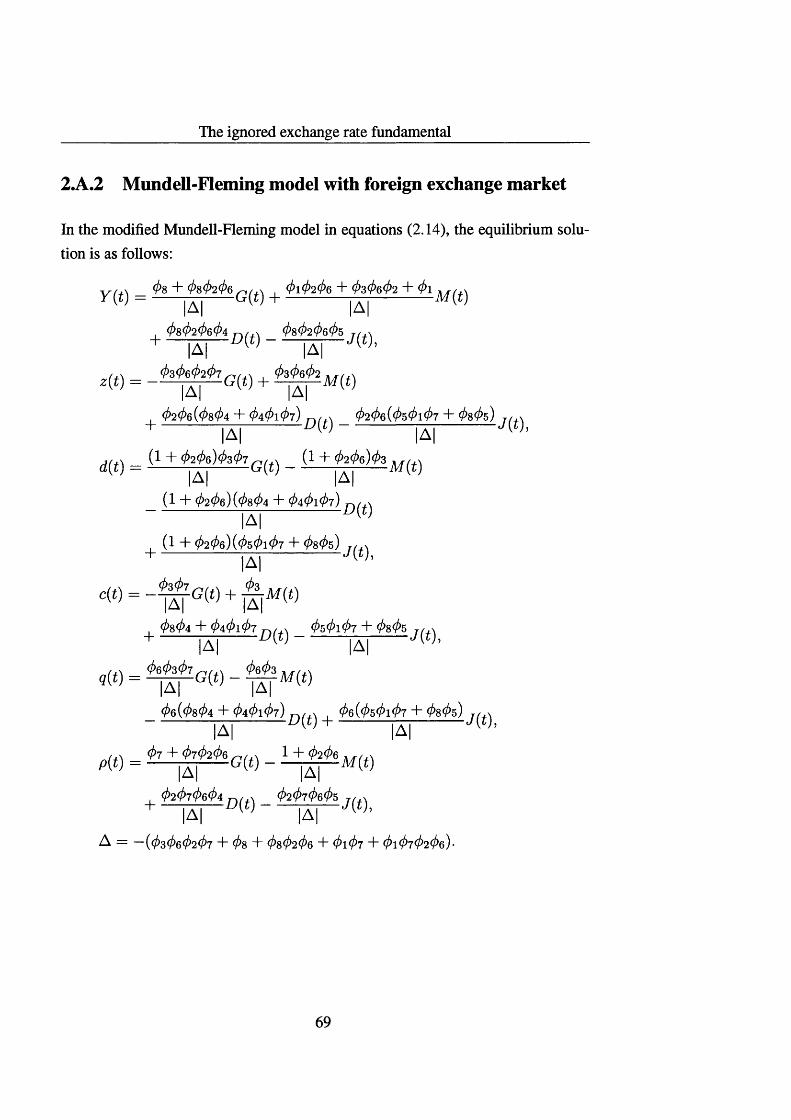
The ignored exchange rate fundamental
2.A.2 Mundell-Fleming model with foreign exchange market
In the modified Mundell-Fleming model in equations (2.14), the equilibrium solution is as follows:
W+\ _ 08 + 080206 , 010206 + 030602 + 01 f ^
W “ ------|A| G(t) + ------------ |A|------------ W, 08020604 08020605
+ |A| { ) |A| { ) ’
2{t) = _ M 0 t G(t) + ^ m
, 0206(0804 + 040107) 0206(050107 + 0805) 7/jA+ |A | [ ) |A | 1
d(t) = ( l + ^ * W 7 G(t) _ ( l + g S ^ j i f (f)
_ (1 + 0206)(0804 + 040107) n /,x |A| U
( (1 + 0206)(050107 + 0805) 7/iA |A|
cW = - ^ G W + A M (i)
, 0804 + 040107 050107 + 0805 rAA+ |A| |A|
9(t) = * j ^ G ( i ) - ^ M ( t )
06(0804 + 040107) 7̂ ^ , 06(050107 + 0805) 7/^[A] 1 j |Aj 1
PW = W
, 02070604 02070605 7/+^|A | 1 j |A | 1
A = —(03060207 + 08 + 080206 + 0107 + 01070206)-
69

The ignored exchange rate fundamental
Nominal Nominal Nominal Tradeexchange exchange exchange balancerate driven rate driven rate driven driven byby current by capital by FX realaccount flows order flow exchange
rateMacro (undergraduate)- Abel / Bemanke (2003)- Blanchard (2003)- Burda / Wyplosz (2001)- Mankiw (2002)Macro (graduate)- Adda / Cooper (2003)- Blanchard / Fischer (1989)- Heijdra / van der Ploeg (2002)- Ljungqvist / Sargent (2004) -Obstfeld/Rogoff (1996)- Romer (1996)- Sargent (1987a)- Sargent (1987/?)- Tumovsky (2000) Development macro- Agdnor / Montiel (1999) International economics- Appleyard / Field (2001)- Copeland (2004)- Hailwood / MacDonald (2000)- Kenen (2000)- Krugman / Obstfeld (2003) Exchange rates- Cheung et al. (n.d.)- Frankel / Rose (1995)- MacDonald (1999a)- MacDonald (1999ft)- Meese / Rogoff (1983a)- Samo / Taylor (2002)- Taylor (1995)FX microstructure- Lyons (2001)
Table 2.1: Exchange rate determinants in economics textbooks. The table lists several assumptions on exchange rate determinants and shows in which economics textbooks and survey articles on exchange rates they are discussed.
70

The ignored exchange rate fundamental
Flow Flexible- Open- Sticky- Realmarket price economy price exchangemodel of monetary IS-LM monetary rateexchange model model model driven byrate (Mundell- (ex prices ofdetermi Fleming change tradablesnation model) rate over vs. non
shooting) tradables
Macro (undergraduate)- Abel / Bemanke (2003) • •- Blanchard (2003) •- Burda / Wyplosz (2001) • • •- Mankiw (2002) •Macro (graduate)- Adda / Cooper (2003)- Blanchard / Fischer (1989) • •- Heijdra / van der Ploeg (2002) • •- Ljungqvist / Sargent (2004)-Obstfeld /Rogoff (1996) • • • •- Romer (1996) • •- Sargent (1987a)- Sargent (1987b)- Tumovsky (2000) •Development macro- Agdnor / Montiel (1999) • •International economics- Appleyard / Field (2001) • • • •- Copeland (2004) • • • •- Hailwood / MacDonald (2000) • • •- Kenen (2000) • • •- Krugman / Obstfeld (2003) • • • •Exchange rates- Cheung et al. (n.d.) • • •- Frankel / Rose (1995) • •- MacDonald (1999a) • • •- MacDonald (19996) • • •- Meese / Rogoff (1983a) • • •- Samo / Taylor (2002) • • •- Taylor (1995) • •FX microstructure- Lyons(2001) • • • • •
Table 2.2: Exchange rate models in economics textbooks. The table lists several models of exchange rate determination and shows in which economics textbooks and survey articles on exchange rates they are discussed.
71

The ignored exchange rate fundamental
Period Change Period Change
1971Q2-1973Q2 +24% 1985Q3-1988Q4 +61%1973Q2-1975Q1 -13% 1988Q4-1990Q2 -20%1975Q1-1976Q4 +6% 1990Q2-1992Q3 +18%1976Q4—1978Q3 +45% 1992Q3-1995Q2 +52%1978Q3-1980Q1 -24% 1995Q2-1998Q3 -35%1980Q1-1981Q1 +25% 1998Q3-2000Q3 +40%1981Q1-1985Q3 +5%
Table 2.3: Large exchange rate movements in Japan. Movements of Japan’snominal effective exchange rate. Source: International Financial Statistics (IMF).
Equilibrium effect US: early 1980s US: mid-1980sG M G T M j G I M T
Y + + T i I Tz — + 1 i T TQ + — T T 1 1P + — T T 1 1
Table 2.4: Mundell-Fleming model. Effects of changes in exogenous variables on the equilibrium outcome in a simple, two-economy version of the Mundell-Fleming model.
Equilibrium effect US: early 1980s US: mid-1980sG M D J G T M j D 1 J T G 1 M t D T J 1
Y + + + 1 4’ 4" 4> 4* 1 1 iz — + + Ar *4 4' 4< 1 1 1 1d + — — + T T T T 1 1 1 1c — + + 4- 4̂ 4' 4" 1 1 1 1Q + — — + T T T T l i l lP + — + 1 1 4* 4" 4' 4- 1 1
Table 2.5: Mundell-Fleming model with foreign exchange market. Effects of changes in exogenous variables on the equilibrium outcome in the Mundell-Fleming model. The model is modified in that it features a foreign exchange market, in which the exchange rate is set in response to currency demands. Accumulating foreign debt becomes an important source of exchange rate pressure.
72

Chapter references
Abel, A. B. andBemanke, B. S. (2003), Macroeconomics, Addison Wesley, Boston, London.
Adda, J. and Cooper, R. (2003), Dynamic Economics: Quantitative Methods and Applications, MIT Press, Cambridge, Mass.
Agenor, P.-R. and Montiel, P. J. (1999), Development macroeconomics, Princeton University Press, Princeton, New Jersey.
Appleyard, D. R. and Field, A. J. (2001), International Economics, McGraw-Hill, Boston.
Balassa, B. (1964), ‘The purchasing power parity doctrine: A reappraisal’, Journal of Political Economy 72(6), 584-596.
Blanchard, O. J. (2003), Macroeconomics, Prentice-Hall International, Upper Saddle River, New Jersey.
Blanchard, O. J. and Fischer, S. (1989), Lectures on Macroeconomics, MIT Press, Cambridge, Mass.
Burda, M. and Wyplosz, C. (2001), Macroeconomics: a European text, Oxford University Press, Oxford.
Bussiere, M. and Mulder, C. (1999), ‘External vulnerability in emerging market economies: How high liquidity can offset weak fundamentals and the effects of contagion’, International Monetary Fund Working Papers (88).
73

Chapter references
Calvo, G. A., Leiderman, L. and Reinhart, C. M. (1996), ‘Inflows of capital to developing countries in the 1990s’, Journal o f Economic Perspectives 10,123— 139.
Cheung, Y.-W., Chinn, M. D. and Garcia Pascual, A. (n.d.), Empirical exchange rate models of the ninetees: Are any fit to survive? Forthcoming.
Copeland, L. (2004), Exchange Rates and International Finance, FT Prentice Hall, Harlow.
Eichengreen, B. (1996), Globalizing Capital, Princeton University Press, Princeton, New Jersey.
Eichengreen, B. (2003), Capital Flows and Crises, The MIT Press, Cambridge, Massachusetts; London.
Eichengreen, B., Rose, A. K. and Wyplosz, C. (1995), ‘Exchange market mayhem: The antecedents and aftermaths of speculative attacks’, Economic Policy 21, 249-312.
Engel, C. (1999), ‘Accounting for US real exchange rate changes’, Journal of Political Economy 107(3), 507-538.
Engel, C. and West, K. D. (2004), ‘Exchange rates and fundamentals’, National Bureau of Economic Research Working Papers (10723).
Evans, M. D. D. and Lyons, R. K. (2003), ‘New micro exchange rate economics’. Unpublished working paper, Haas School of Business, UC Berkeley.
Flood, R. P. and Garber, P. M. (1984), ‘Collapsing exchange-rate regimes: some linear examples’, Journal of International Economics 17(0), 1-13.
Frankel, J. A. (1984), ‘The yen/dollar agreement: Liberalizing Japanese capital markets’, Policy Analyses in International Economics (Institute for International Economics) (9).
Frankel, J. A. (1985), ‘The dazzling dollar’, Brookings Papers on Economic Activity (1), 199-217.
74

Chapter references
Frankel, J. A. and Rose, A. K. (1995), An empirical characterization of nominal exchange rates, in Grossman and Rogoff (1995), pp. 1689-1729.
Girton, L. and Roper, D. (1977), ‘A monetary model of exchange market pressure applied to the postwar Canadian experience’, American Economic Review 67(4), 537-548.
Grenville, S. A. (1998), ‘Capital flows and crises’, Reserve Bank of Australia Bulletin .
Grossman, G. M. and Rogoff, K., eds (1995), Handbook o f International Economics, Vol. 3, North Holland, Amsterdam.
Hailwood, R and MacDonald, R. (2000), International Money and Finance, Black- well, Malden, MA.
Hau, H. and Rey, H. (2003), ‘Exchange rates, equity prices and capital flows’, Centre for Economic Policy Research Discussion Papers (3735).
Heijdra, B. J. and van der Ploeg, F. (2002), Foundations of Modem Macroeconomics, Oxford University Press, Oxford, New York.
Hooper, P. and Morten, J. E. (1982), ‘Fluctuations in the dollar: a model of nominal and real exchange rate fluctuations’, Journal o f International Money and Finance 1, 39-56.
Isard, P. and Stekler, L. (1985), ‘U.S. international capital flows and the dollar’, Brookings Papers on Economic Activity (1), 219-236.
Kenen, P. B. (2000), The International Economy, Cambridge University Press, Cambridge (United Kingdom), New York.
Kouri, P. J. K. (1976), ‘The exchange rate and the balance of payments in the short run and in the long run: A monetary approach’, Scandinavian Journal o f Economics 78, 280-304.
Krugman, P. R. (1979), ‘A model of balance-of-payments crises’, Journal o f Money, Credit, and Banking 11(3), 311-325.
75

Chapter references
Krugman, P. R. (1985), Is the strong dollar sustainable?, in Federal Reserve Bank of Kansas City, ed., ‘The U.S. Dollar: Recent Developments, Outlook, and Policy Options’, pp. 103-132.
Krugman, P. R. (1991), Has the adjustment process worked?, in C. F. Bergsten, ed., ‘International Adjustment and Financing’, Institute for International Economics, Washington, DC.
Krugman, P. R. (1999), ‘Balance sheets, the transfer problem, and financial crises’, International Tax and Public Finance 6,459-472.
Krugman, P. R. and Obstfeld, M. (2003), International Economics, Addison Wesley, Boston.
Ljungqvist, L. and Sargent, T. J. (2004), Recursive Macroeconomic Theory, MIT Press, Cambridge, Massachusetts; London.
Lyons, R. K. (2001), The Microstructure Approach to Exchange Rates. Forthcoming, Fall 2001, MIT Press.
MacDonald, R. (1999a), ‘Exchange rate behaviour: Are fundamentals important?’, The Economic Journal 109, 673-691.
MacDonald, R. (1999b), What do we really know about real exchange rates?, in R. MacDonald and J. L. Stein, eds, ‘Equilibrium Exchange Rates’, Kluwer Academic Publishers, Boston, Dordrecht and London, pp. 19-65.
Machlup, F. (1939), ‘The theory of foreign exchanges’, Economica 6(24), 375-397.
Machlup, F. (1940), ‘The theory of foreign exchanges’, Economica 7(25), 23-49.
Mankiw, N. G. (2002), Macroeconomics, Worth Publishers, New York.
McKinnon, R. I. and Pill, H. (1997), ‘Credible economic liberalizations and overborrowing’, American Economic Review 87(2), 189-193.
Meese, R. and Rogoff, K. (1983a), ‘Empirical exchange rate models of the seventies: Do they fit out of sample?’, Journal o f International Economics 14,3-24.
76

Chapter references
Meese, R. and Rogoff, K. (19836), The out-of-sample failure of empirical exchange rate models, in J. A. Frenkel, ed., ‘Exchange Rates and International Macroeconomics’, Chicago University Press, Chicago.
Mussa, M. (1979), ‘Empirical regularities in the behavior of exchange rates and theories of the foreign exchange market’, Camegie-Rochester Conference Series on Public Policy 11, 9-57.
Obstfeld, M. (1986), ‘Rational and self-fulfilling balance-of-payments crises’, American Economic Review 76(1), 72-81.
Obstfeld, M. (1994), ‘The logic of currency crises’, Cahiers Economiques etMon- etaires (43).
Obstfeld, M. and Rogoff, K. (1995), The intertemporal approach to the current account, in Grossman and Rogoff (1995), pp. 1731-1799.
Obstfeld, M. and Rogoff, K. (1996), Foundations o f International Macroeconomics, MIT Press, Cambridge, Massachusetts.
Obstfeld, M. and Rogoff, K. (2000), Perspectives on OECD economic integration: Implications for US current account adjustment.
Obstfeld, M. and Rogoff, K. (2004), ‘The unsustainable US current account position revisited’, National Bureau of Economic Research Working Papers (10869).
Robinson, J. (1937a), ‘Essays in the theory of employment’.
Robinson, J. (19376), The foreign exchanges, in Essays in the Theory o f Employment (Robinson, 1937a).
Rogoff, K. (2002), ‘The failure of empirical exchange rate models: No longer new, but still true’, Economic Policy Web Essays .
Romer, D. (1996), Advanced Macroeconomics, McGraw-Hill.
Rosenberg, M. R. (1996), Currency Forecasting. A Guide to Fundamental and Technical Models o f Exchange Rate Determination, Irwin, London, Chicago, Singapore.
77

Chapter references
Salant, S. W. and Henderson, D. W. (1978), ‘Market anticipations of government policies and the price of gold’, Journal of Political Economy 86(4), 627-648.
Samuelson, P. A. (1964), ‘Theoretical notes on trade problems’, Review of Economics and Statistics 46, 145-154.
Sargent, T. J. (1987a), Dynamic Macroeconomic Theory, Harvard University Press, Cambridge, Mass., London.
Sargent, T. J. (1987&), Macroeconomic Theory, Academic Press, New York.
Samo, L. and Taylor, M. P. (2002), The Economics o f Exchange Rates, Cambridge University Press, Cambridge.
Taylor, A. M. (2002), ‘A century of current accout dynamics’, Journal o f International Money and Finance 21, 725-748.
Taylor, M. P. (1995), ‘The economics of exchange rates’, Journal of Economic Literature 33(1), 13-47.
Tesar, L. L. and Wemer, I. M. (1995), ‘Home bias and high turnover’, Journal of International Money and Finance 14(4), 467—492.
Tumovsky, S. (2000), Methods of Macroeconomic Dynamics, MIT Press, Cambridge, Massachusetts.
Wang, Y. (2002), ‘Capital account liberalization: The case of Korea’.
Williamson, J. (1985), The Exchange Rate System, Institute for International Economics, Washington, DC.
78

Chapter 3
Balance of payments accounting and exchange rate dynamics
In this chapter, I analyze in detail the implications of the balance of payments accounting identity for the dynamics of international payment flows and exchange rates. To my knowledge, no other study has ever looked at the effects of trade and capital flows on currency movements in a comparable fashion. As the previous chapter showed, mainstream exchange rate models ignore the role of trade and capital flows for exchange rate determination altogether. But even the traditional flow market model of the exchange rate has significant shortcomings as it lacks a dynamic perspective and fails to recognize the dynamic interrelatedness—due to the balance of payments accounting identity—of the movements of the current account, the capital account and international payments.
3.1 Introduction
The chapter aims to demonstrate how balance of payments imbalances influence the demands for different currencies in the foreign exchange market over time. To this end, a dynamical system approach is developed, which allows to assess how
The paper on which this chapter is based has been presented at the International Financial Stability Programme at the CEP (LSE).
79

Balance of payments accounting and exchange rate dynamics
international payments evolve for different sets of assumptions regarding the joint dynamic behaviour of various balance of payments components. This chapter focuses in particular on the adjustment delay, a phenomenon that, as the previous chapter has demonstrated, is of considerable empirical importance.
Specifically, the following scenarios are analyzed in this chapter: First, the situation is studied where current account transactions, such as exports and imports, are paid for directly, assuming away other capital account transactions such as trade credits or debt and equity flows. These assumptions serve as a benchmark to illustrate the limited amount of capital mobility between major industrialized economies before the removal of capital controls in the 1970s and 1980s. In this and all following setups, or scenarios, I assume that the real exchange rate depends on the excess holdings of different currencies in the foreign exchange markets. In addition, I assume that the Marshall-Lemer condition holds and that the current account adjusts over time to changes in the real exchange rate. Under these very basic and realistic assumptions, I demonstrate how initial current account imbalances can lead to long-lasting swings in both the current account and the real exchange rate.
In a second setup, I analyze the situation where current account transactions are in part financed by debt. This carries the implication that payment flows are delayed, with the result that the impact of current account movements on the exchange rate is spread out over a longer horizon. Whereas the current account and the exchange rate still move in a cyclical fashion, the lag between both variables becomes longer. It is shown that this setup represents very well the experience of the Japanese balance of payments and exchange rate over the past three and a half decades, as well as for instance Germany’s performance during its volatile export boom of the 1980s.
A third constellation studied in the chapter examines the effect of temporary, autonomous capital inflows into a country. I show that under sensible assumptions, such inflows provoke a temporary appreciation of the currency even when the current account is strongly deteriorating. The model replicates the experience of the United States during the 1980s when the US dollar appreciated massively despite the fact that the US external deficit was reaching record levels (similar to the developments there in the late 1990s and early 2000s).
In a further variation of the model, the chapter considers the case of a country with a fixed exchange rate. It analyzes how payment flows into and out of the
80

Balance of payments accounting and exchange rate dynamics
country evolve in response to trade and capital flows, and how the stock of foreign exchange reserves of the country is affected. It is then shown in a simulation how temporary inflows of foreign capital can lead to a deterioration of the current account balance and a build-up of foreign claims, which eventually leads to the depletion of reserves and a breakdown of the currency. This dynamic pattern can be generated under rather simple assumptions within the dynamical system framework described above. It corresponds well with anecdotal evidence from countries hit by currency crises. This is illustrated by a case study of the Korean economic performance before and during the Asian crisis of 1997-1998.
Finally, the same framework is used to demonstrate how a crawling peg can help to avoid a currency crisis and to maintain relative exchange rate stability. Particularly in countries suffering from high inflation, introducing an exchange rate anchor can be a promising strategy to reduce inflation. However, adopting a hard peg also carries its risks, in particular if it takes time for inflation to fall. The chapter shows why it has made sense for countries such as Israel, Poland and Turkey to opt for crawling pegs or bands in the past (possibly as an intermediate step before moving on to a full float of the currency).
Plan of the chapter. The chapter is organized as follows: Section 3.2 explores how currency supplies in the foreign exchange market evolve over time and how the excess demands and supplies in that market affect the exchange rate. Section 3.3 makes further assumptions regarding the impact of the exchange rate on the current account and the way in which trade and capital flows react to movements of each other. Based on the theoretical framework, section 3.4 shows how current account and exchange rate movements evolve jointly over time. This section then analyzes how debt flows and other capital flows affect the dynamic pattern of the current account and the exchange rate. It also takes a closer look at currency crises and the capacity of crawling pegs to prevent such crises. Section 3.5 discusses the wider implications of the model for some central issues in international economics.
Notation. In the course of this chapter, we will need to refer to a number of variables, as we will be concerned not only with balance of payments flows, but also with the time derivatives of those flows and with accumulated stocks of foreign assets. We will also need to refer to variables that can be denominated in different
81

Balance of payments accounting and exchange rate dynamics
currencies. So as to make it easier for the reader to get familiar with the notation in this chapter, table 3.1 on page 126 provides an overview of the relevant variables and subscripts.
In our analysis, we employ five variables to represent different types of balance of payments flows: a current account variable, z(t), which matches the usual current account definition; a variable capturing autonomous capital flows, k(t), which will be defined in more detail later on; a debt flow variable, d(t); a variable representing international cash flow, c(t); and finally, a variable corresponding to flows of international reserves, r(t). Table 3.2 on page 127 indicates how each of these variables relate to the published balance of payments statistics.
3.2 Exchange rate determination
How are exchange rates determined? The hypothesis that we shall adopt here is possibly the most simple and intuitive: The exchange rate is driven by the demands and supplies of currencies in the foreign exchange market, which depend on the need of foreign and domestic agents to obtain each others’ currencies. Currency demands, in turn, are influenced by the different types of transactions that economic agents undertake.
3.2.1 The balance of payments and international cash flow
A natural way to start is by looking at examples that show how balance of payments transactions influence international currency flows.
Example: Exports and imports
Consider the case in which country 1 (Home) exports goods to country 2 (Foreign) that are paid for immediately. In the accounting framework of table 3.3 on page 128, this transaction is labelled T1. The value of those exports equals their volume times their price, denoted Pi2 \iZi2 - Country 1 therefore receives a cash payment of a corresponding amount from country 2, denoted C2 \\\. In the balance of payments
82

Balance of payments accounting and exchange rate dynamics
of country 2, the same transaction T1 is recorded as an import of value S2\iP2 i\2 ^2 i and the associated payment is denoted as S211C1212. Note that we decide to record the balance of payments transactions of each country in its own respective currency.
Table 3.3 also records a second transaction, T2, which corresponds to imports by country 1 from country 2. Of course, the entries in the balance of payments of both countries are quite analogous.
The interesting part of table 3.3 is the third one, which records the flows of assets and liabilities in the foreign exchange market. The foreign exchange market is the place where currencies are exchanged at their respective exchange rate. It can be located in country 1 or country 2 or elsewhere.
When the foreign exchange market supplies currency of a given country to economic agents, this is recorded as a credit item in the accounts of table 3.3. Similarly, when the foreign exchange market receives payments, this is recorded as a debit item. Considering therefore our two examples, the export transaction (Tl) leads to an decrease in the net holdings of currency 1 and to an increase in the net holdings of currency 2 in the foreign exchange market. The import transaction (T2), on the other hand, has just the opposite effects.
Now we make an important assumption:
Assumption 1 (Home bias in money holdings). Economic agents hold only the currency o f their own country. They convert foreign currency into domestic currency immediately.
A very similar assumption is made for instance by Hau and Rey (2003) in their study of exchange rate effects of capital flows. It is not entirely realistic, though, given that for instance the US dollar is widely held abroad. In recent decades, there has also been an increase in the international demand for other major currencies, including the yen (Das, 1993). Nevertheless, assumption 1 can be justified by the fact that, by and large, the home bias for currency holdings remains very significant for most currencies.
Assumption 1 implies that the export transaction Tl will lead to an increase in the demand for currency 1 and in the supply of currency 2 in the foreign exchange market. Conversely, the import transaction T2 will lead to an increase in the supply
83

Balance of payments accounting and exchange rate dynamics
of currency 1 and in the demand for currency 2. Note that each transaction has two separate effects since it affects the demand conditions of each of the two currencies.
In the above, we have made one implicit assumption:
Assumption 2 (Currency denomination of balance of payments transactions).Balance of payments transactions are denominated in the currency of the country receiving the associated payment. Exports for example are invoiced in the currency of the exporter. Foreign debt is denominated in the currency o f the borrower.
This assumption is made for convenience to avoid having to consider different currency denominations. However, it should not be overlooked that in the following analysis currency denomination generally matters.
Example: Foreign borrowing and lending
Capital flows generate international payment flows, too. As an example, table 3.4 on page 128 displays the transactions associated with international debt flows. With transaction T3, country 1 borrows money from country 2, and this leads to an increase in the demand for currency 1 and in the supply of currency 2 in the foreign exchange market. Transaction T4, on the other hand, implies that country 1 lends money to country 2, which increases the supply of currency 1 as well as the demand for currency 2.
3.2.2 The foreign exchange market
Now that we have seen how the demands and supplies for currencies in the foreign exchange market are affected by countries’ commercial and financial dealings, we can turn to the question of how the foreign exchange market sets the exchange rate. Since the market carries out all currency conversions resulting from countries’ balance of payments transactions, its currency holdings generally do not balance to zero; in other words, the market does not clear. We shall assume that the price, or value, of a currency falls with the foreign exchange market’s net holdings of that currency and vice versa. The exchange rate between two currencies is given by the ratio of the two currencies’ prices.
84

Balance of payments accounting and exchange rate dynamics
More specifically, suppose that the value of country l ’s currency, Vi(t), is given by the inverse of the country’s price level—that is, its domestic value in the absence of exchange market pressure—times an index measuring the excess demand for currency 1 in the foreign exchange market:
The demand index is modelled as an exponential function of the exchange market’s cumulative holdings of country l ’s currency, after normalization of the latter by country 1 ’s price level. A proportional increase in the demand for currency 1 has thus the same effect as a decrease in the supply of the same proportion. The normalization by the price level ensures the comparability of the index across currencies.
Currency 2’s value, V2 (t), is determined analogously:
(3.1a)
where
(3.1b)
where
The nominal exchange rate between both countries, Si 12(f), is then given by the ratio of V\ (t) and V ^):

Balance of payments accounting and exchange rate dynamics
The real exchange rate is therefore given by:
«'»<•>Ci(t)C2(t)
= exp J ((PiW )-1 + (-P2(«))_15i|2(r)) c2i|i(r)dr^
X 6XP ( _ I / ((■PlW )~1,S2l1(r ) + (A W )-1) Ci2|2(i-)<ir ̂ .
(3.3)
To see how the real exchange rate, Qi|2(£)> changes over time, we take the time derivative:
2 Q l|2 ft)
£ X Q l|2(«)
= [(A W )-1 + (A W )- i SipW] C2H1W (3 4)
- [(A W )-1SiiiW + (A W )"1] cupW
A W r M I A W r M 2 (PiW )2 1 2(Pb(t))2 12
International cash flow—here given by c2\\\(t) and Ci2|2 (^)—is thus a central determinant of the exchange rate. The price levels of both countries matter for the exchange rate, too, since they directly influence the value of each respective currency. Finally, note that equation (3.4) implies that exchange rate fluctuations reinforce themselves: When the exchange rate appreciates, foreign demand for the domestic currency rises whereas domestic demand for the foreign currency falls, pushing the home currency up even further. This could for instance help to explain the fact that currencies tend to fall precipitously following the breakdown of exchange rate pegs.
For later purposes, it will be useful to work with a simplified version of equation (3.4). Since our main interest is to analyze the effects of currency flows on
86

Balance of payments accounting and exchange rate dynamics
exchange rates, we assume that P\(t) = P2 M = 1- Equation (3.4) thus simplifies to:
Consequently, assuming that S^2(t) = S2̂ (t) = 1 and c\(t) = c*12\2(t) — c21̂ (t) = 0, the change of the real exchange rate depends simply on international cash flow:
<7l|2(f) « (Cl2|2(f) - C2l|l(f))
= -eci(f).
Expectations
The foreign exchange market tends to be highly speculative. Market participants make strong efforts to forecast future economic developments, but this does not mean that they are by and large successful. Here, we are making the following assumption:
Assumption 3 (No knowledge of the future). Economic agents are ignorant of the future.
Assumption 3 is but a good description of reality. Cheung and Wong (2000) have recently carried out a survey of foreign exchange traders’ views on exchange rate dynamics. According to the survey, four out of five practitioners in the interbank foreign exchange markets in Hong Kong, Singapore and Tokyo considered economic fundamentals to be a significant determining factor of exchange rates in the long run (over an horizon of more than six months). Nevertheless, only between
- X qi\2(t) — [ l + S l |2 ( t ) ] C21|l(£) — [ l + *] Ci2|2(£)- (3.5)
Equation 3.5 can be linearized around 5Jj2(t), c\212 and c21̂v to yield:
« [1 + SJ|2(£)] (P2i|i(t) - 4i\i(t))~ t1 + (STpW)-1] (C12|2 W - c*12l2{t))
+ [C21|lW — C12|2(^)( ^112W ) 2] — jS'i|2(£)) •
(3.6)
87

Balance of payments accounting and exchange rate dynamics
22% (Tokyo) and 27% (Singapore) of the respondents believed that exchange rates were at all predictable over that horizon.
Moreover, it is interesting to note that well-known papers in the macroeconomic literature are based on hypotheses that are very similar to assumption 3. For example, in the seminal currency crisis models by Krugman (1979) and Hood and Garber (1984), the future path of the economy is certain. The rate of domestic credit growth is given and speculators with perfect foresight can foresee with precision the moment in which the country will run out of reserves and in which the currency will collapse. Selling the currency and waiting for the collapse is a one-way bet, even if the shadow exchange rate moves above the fixed rate in the meantime, since it must eventually fall below the peg. However, Krugman and Hood and Garber rule out the possibility of an anticipated attack. What they are (implicitly) assuming is that speculators can only foresee the very next instant.
3.3 Balance of payments dynamics
We have so far specified how balance of payments transactions determine international cash flow and how international cash flow drives the exchange rate. To complete our model, we need to describe how the various balance of payments components evolve over time and, in particular, how they are affected by exchange rate movements.
3.3.1 Current account
Regarding the movements of the current account, we make a fundamental assumption:
Assumption 4 (Gradual current account adjustments). Current account adjustments occur gradually over time.
To many, this assumption would immediately seem plausible. Therefore, I leave it with an elegant quote from Keynes’s (1929) article on the Transfer Problem:
88

Balance of payments accounting and exchange rate dynamics
My own view is that at a given time the economic structure of a country, in relation to the economic structures of its neighbours, permits of a certain "natural" level of exports, and that arbitrarily to effect a material alteration of this level by deliberate devices is extremely difficult. [...]In the case of German Reparations, on the other hand, we are trying to fix the volume of foreign remittance and compel the balance of trade to adjust itself thereto. Those who see no difficulty in this [...] are applying the theory of liquids to what is, if not a solid, at least a sticky mass with strong internal resistances.
Real exchange rate
We shall assume that the real exchange rate is the major driving force behind the trade balance and therefore behind the current account. An appreciated real exchange rate leads to a deterioration of a country’s international competitiveness and thus puts a downward pressure on the trade balance; a weak real exchange rate, on the other hand, strengthens the trade balance:
z(t) = -4>iz(t) - faq1]2(t)(3.oa)
= -<t> 1 (z(t) - z( t ) ) ,
where
= -^ 9 l |2 (0 -
The variable z(t) is the equilibrium value of the current account, which depends on the real exchange rate, qi\2 (t).
The parameter (j>i determines the speed with which the current account reverts to equilibrium, whereas the parameter ratio measures the exchange rate sensitivity of the current account. As we will see in chapter 6, exchange rate fluctuations can influence the current account’s trend significantly. By comparison, the economic forces that push the current account towards equilibrium appear to be relatively small in general. Obstfeld and Rogoff (1996, page 67) mention the examples of Australia and Canada, two countries that have run persistent current account
89

Balance of payments accounting and exchange rate dynamics
deficits over the last one and a half centuries for which data exist (see figure 3.13). Between 1950 and 1994 for instance, Australia’s current account was in deficit in all but four years, while Canada’s was in deficit in all but five. This example illustrates why we shall choose the parameter fa to be rather small in our later simulations.
Foreign investment
International capital flows are another important driving force behind the current account. Worldwide, there are many examples of countries that experienced large international capital inflows in the past—say, after successful stabilization measures or as a result of promising investment opportunities—and who subsequently observed substantial declines in their current account balances (Grenville, 1998; Mon- tiel and Reinhart, 2001; Eichengreen, 1990). In many cases, capital inflows resulted in domestic consumption and investment booms, widening the gap between national savings and investment.
McKinnon and Pill (1997) provide some such examples:
The policy reforms favouring free trade, privatization, deregulation of domestic industry, and fiscal consolidation pursued by Chile in the mid- 1970s led to massive capital inflows through 1981, followed by a financial crash and economic downturn during 1982-1983. In Mexico after 1988, similarly comprehensive real-side reforms attracted large capital inflows, which suddenly reversed during the December 1994 financial panic and steep 1995 downturn. Argentina currently faces the depressed aftermath of a reform program during which it borrowed too much and subsequently had to retrench.
This pattern is not confined to developing countries. After a dismal period of high inflation and public intervention in Britain in the 1970s, the Thatcher government undertook apparently successful industrial restructuring and fiscal consolidation in the early 1980s. Enthusiasm for Britain’s changed economic prospects attracted capital inflows, increased consumption, and triggered a boom in residential and commercial real estate in the late 1980s that culminated in the bust of the early 1990s.
90

Balance of payments accounting and exchange rate dynamics
And finally comes the exception, which turns out not to be one (the article by McKinnon and Pill (1997) was published in May 1997, just before the outbreak of the Asian crisis):
Nevertheless, not all liberalizing countries attracting large capital inflows need experience this boom-and-bust cycle. Indonesia, Malaysia, and Thailand have all had current-account deficits of 5-8 percent of GNP (similar to Mexico before the fall) for almost a decade, without a Mexico- or Chile-type debacle. These East Asian economies achieved virtual steady-state growth with high saving and very high investment, although doubts about its quality could yet provoke a cutback in lending.
In all the examples mentioned, the recipients of capital inflows—that is, Chile, Mexico, Britain, Indonesia, Malaysia, Thailand—were all experiencing large and increasing current account deficits.
Such boom-and-bust cycles, in which the current account gradually worsens in response to a surge in capital inflows, can be readily derived from standard open economy models (Calvo et al., 1996). In an intertemporal model of consumption and saving in an open economy with capital mobility, a fall in the world interest rate will induce substitution and (in the case of a debtor country) income effects, which will result in a consumption boom and a widening current account deficit. These effects could become even stronger if the country was initially credit rationed, or if it owed debt with a variable interest rate. In a model with endogenous investment, the interest rate shock could also translate to a rise in investment, widening the current account further.
We shall refer to such foreign investment flows as autonomous capital flows, denoted as k(t), to distinguish them from other capital flows, discussed below, whose purpose it is just to finance existing current account imbalances. To incorporate autonomous capital flows into our dynamic framework, we can rewrite the differential equation describing the behaviour of the current account:
z(t) = -</>iz(t) - </>2<7i|2(£) - faKt)- (3-8b)
91

Balance of payments accounting and exchange rate dynamics
For models in which autonomous capital flows play a role, we will use equation (3.8b) rather than equation (3.8a).
3.3.2 Capital account
Whereas the current account is set to evolve gradually, we assume that the adjustment on the financial side of the balance of payments has two components, respectively labelled "accommodating" and "autonomous". Under normal circumstances, current account imbalances are financed by "accommodating" capital flows. However, there may be times when a country attracts more or capital flows than strictly needed, as in the examples above of countries that experienced overborrowing episodes in the past. In this case, we shall talk of "autonomous" capital flows.
We make the following assumption:
Assumption 5 (Accommodating capital flows). Accommodating financial flows that are needed to finance current account imbalances occur instantaneously.
This assumption really just follows from the definition of accommodating and autonomous capital flows above. Nevertheless, this is a good opportunity to quote Keynes (1929) once more, who said:
Historically, the volume of foreign investment has tended, I think, to adjust itself—at least to a certain extent—to the balance of trade, rather than the other way round, the former being the sensitive and the latter the insensitive factor.
However, this leaves us with the question: How does a country finance a deficit in its balance on current account; or conversely, how does it invest a balance of payments surplus? What we shall assume here is that current account imbalances are financed mainly through international debt and lending and to some extent through direct monetary payments.
There is considerable empirical evidence indicating that countries’ international portfolios are in large part made up by fixed-income investments. For instance, Kraay, Loayza, Serven and Ventura (2000) have recently shown that gross foreign
92

Balance of payments accounting and exchange rate dynamics
asset positions in a worldwide cross section of countries consist mostly of foreign loans rather than foreign equity. This implies that deficit countries cover their foreign investment needs primarily by means of borrowing from abroad; surplus countries, on the other hand, choose lending over other forms of foreign investment. Probably the best example for the latter is Japan, the world’s largest creditor nation, as we already saw in section 2.2.1: Starting with the opening of its capital account in the late 1970s and early 1980s, the country has over a long time been investing a relatively stable fraction of its surpluses in debt securities abroad, mainly in the United States. The strong correlation between Japan’s current account and its debt securities balance, which we observed in figure 2 .6 , implies that the fluctuations of other components of the Japanese capital account effectively cancelled each other out over many years.
The debt balance in the balance of payments, which we denote as d(t), is thus determined as follows:
d(t) = — (1 — oi)(z(t) + k(t)) — 7 f e_7^_T̂ d(r)dr. (3.9)Jo
This equation says that international lending always covers a fraction (1 — a) of a country’s external financing requirement, which is defined here as the current account net of autonomous capital flows. The debt balance also includes all repayments of previously incurred debt in the current period, which are captured by the integral in equation (3.9).
Note that the maturity structure of foreign debt is assumed constant over time; it is given by an exponential function, which turns out to be analytically convenient since it allows us to easily calculate the Laplace transform of the integral in equation (3.9) . 1
!Let f ( t ) = exp(—7 (f)) and let h(t) denote the integral in equation (3.9). Notice that h(t) is the convolution of f ( t ) and d(t), denoted ( / * d)(t). Then by the convolution theorem (Kreyszig, 1999; Stroud and Booth, 2003), the Laplace transform H( s ) = L{h(t ) } of the convolution h(t) is the product of the Laplace transforms F(s) = L { f ( t ) } and D( s ) = L{d( t ) } of f ( t ) and d(t) respectively. In our case therefore, H( s ) reduces to the simple expression 7 D(s) / ( s + 7 ), which facilitates our further analysis considerably.
93

Balance of payments accounting and exchange rate dynamics
3.3.3 Cash flow
Note that the balance of payments identity in our model can be stated as:
z(t) + k(t) + d(t) + c(t) + r(t) = 0 , (3.10)
where r(t) denotes the official sales of foreign reserves. Absent official intervention in the foreign exchange market, international payment flows, c(t), are driven by the sum of a country’s current account and its financial balance:
However, when a country wants to stabilize its exchange rate, it needs to offset any cross-border payment flows since these would, according to equation (3.7), affect the exchange rate. The net quantity of foreign reserves that the authorities need to sell in this case is therefore:
Again, assumption 3 is quite important here. Since people are ignorant regarding the future, they cannot foresee the effect of their international payments on the exchange rate and all its possible macroeconomic consequences. Instead, they simply make their payments for individual balance of payments transactions when they are due. For example, when people buy cars abroad or invest in foreign bonds, they normally just pay the money and worry little about the timing of the required currency conversion. Firms and banks, who have better macroeconomic oversight, might be more rational when carrying out currency transactions. However, even their behaviour is likely far from forward-looking or optimal. According to the survey by Cheung and Wong (2000) that has already been mentioned, even foreign exchange traders, who tend to believe that exchange rates are driven by economic fundamentals over the longer term, consider exchange rates to be by and large unpredictable. Therefore, even if economic agents tried to optimize their international cash flow by making forward-looking decisions, they would probably miss their own objective most of the time.
c(t) = — z(t) — k(t) — d(t). (3.11)
r(t) = — z(t) — k(t) — d(t). (3.12)
94

Balance of payments accounting and exchange rate dynamics
3.4 Explaining patterns of exchange rate behaviour
In this section, we will study the interaction of balance of payments and exchange rate movements under different economic conditions. We will analyze different economic models, which all share the common assumptions that were laid out in the previous two sections.
The models that we study consist of systems of differential equations, which are solved using Laplace transforms. As a consequence, we are able to derive solutions in analytic form for all our models. However, even rather simple-looking dynamical systems turn out to have solutions that look quite overwhelming; those solutions are typically of little use for understanding the dynamic evolution of the system. Instead of writing down the explicit solutions, we shall prefer to plot the variables of the solved systems over time, based on an appropriate choice of parameters and initial conditions. Unless stated otherwise, we assume s(0) = 0 and 2 (0 ) = 0 as our initial conditions. For all of our models, we adopt the following parameter specification:
The choice of parameters is certainly ad-hoc and somewhat subjective. However, the values were chosen so as to produce plausible economic interactions and there is reason to believe that the conclusions to which they lead are quite representative.
3.4.1 International cash flow
Let us start with a setup in which current account transactions, such as exports and imports, are paid for straight away in cash, that is, by direct monetary payments. Any other capital account transactions, including trade credits or purchases of foreign debt or equity securities, are excluded from the model; they either do not take place or net out to zero.
£ = 0.1,
0 3 = 0.1,
0i = 0.03,
a = 0 . 1,
02 = 0.06, 7 = 0.05.
95

Balance of payments accounting and exchange rate dynamics
Model
As discussed above, the cash flow variable, c(t), drives the nominal exchange rate, s(t), and thus the real exchange rate, q(t) (since it is assumed that price levels at home and abroad are constant and normalized to one):
Q1\2 (t) = -£c(t). (3.13a)
The movements of the current account and the exchange rate simply mirror each other in this model:
z(t) = -<j>!z(t) - ^29l|2(t),(3.13b)
c{t) = -z( t ) .
In this particular setup, a different initial condition is chosen for the current account variable, namely z(0) = 1. This is necessary in order to set the system in motion.
Simulation
Figure 3.1 shows that this model produces long, cyclical current account movements, whose amplitude declines over time.2 The graph reminds of the long swings in the balance of payments and exchange rate data from Japan and Germany, which we saw in earlier chapters.
In this model, the cyclical fluctuations come about since current account imbalances immediately produce offsetting payment flows, which push the exchange rate either up or down, depending on whether the current account is in surplus or in deficit. Any current account imbalance thus carries with it the seed of its own reversal. The interaction between the current account and the exchange rate is plotted in figure 3.2, and one can easily spot the lagged adjustment of the exchange rate, which is similarly encountered in the real-world examples of the earlier chapters.
2Note that in this and all the following models, a unit of time, t, corresponds to a period of, say, a week and a month.
96

Balance of payments accounting and exchange rate dynamics
— 1e o 8 0 1 O O 1 2 0 1 4 0
t
current account cash flow
Figure 3.1: A basic model of cash flow: balance of payments dynamics. Simulation of the joint dynamic behaviour of the current account and cash balances in a model in which exports and imports are paid for in cash, for chosen parameters and initial values.
Foreign exchange intervention
In the real world, it is unlikely that official authorities would simply stand by and watch when the current account and exchange rate start to fluctuate strongly. To counteract a current account imbalance is not an easy matter. However, as far as exchange rate movements are concerned, the most obvious remedy is to intervene in the foreign exchange market.
When we look again at our example of Japan, we see that this is indeed what has been going on there over the past three decades. Figure 3.3 on page 99 plots the purchases of official reserves against the real effective exchange rate as well as against the percentage changes of the exchange rate. In the upper panel, official intervention appears to be rather uncorrelated with the level of the exchange rate. However, in the lower panel, we can observe a considerable correlation between the official acquisition of reserves and the contemporaneous appreciation of the Japanese exchange rate. According to the model above, any appreciation of the
97

Balance of payments accounting and exchange rate dynamics
0.8
0.6
— 0.66 0 8 0 1 O O 1 2 0 1 4 0
t
current account exchange rate
Figure 3.2: A basic model of cash flow: current account and exchange rate. Simulation of the interaction between current account and exchange rate movements in a model in which exports and imports are paid for in cash, for chosen parameters and initial values.
yen must stem from Japan’s incoming payments, and this suggests that in the past Japan’s authorities have continually been trying to offset some of those payment flows by purchasing foreign reserves from abroad.
It is rather straightforward to adapt the above model in order to include official intervention. Suppose the authorities followed a rule whereby they always buy foreign exchange reserves so as to offset a constant fraction of the cash flow that would occur in the absence of intervention. The cash flow variable in the model would then become accordingly lower. However, the swings in the balance of payments and in the exchange rate would continue to occur, only that exchange rate changes would come about more slowly and that the cycle period would become longer.
98

Balance of payments accounting and exchange rate dynamics
| g73 ^1 ? O •?
(a) +
++ + •4-_ + +
+ -»■+
++
1 . . . . 1 . . . i . . 1 . . . . i . . . . 1 i . . . . i . . . . i .4.20 4.25 4.30 4.35 4.40 4.45 4.50 4.55 4.60
(b) Real exchange rate
w+ + ,
+ ++ +
* +
- ♦
-0.125 -0.100 -0.075 -0.050 -0.025 0.000 0.025 0.050 0.075 0.100 0.125Real exchange rate change (appreciation in percent)
0.150 0.175 0.200
Figure 3.3: Japan’s foreign exchange intervention. Cross plots of Japanese officialreserve intervention (in billions of US dollar) and, respectively, Japan’s real effective exchange rate (based on the WPI, upper panel) and its real effective exchange rate appreciation (based on the WPI, in percentage terms, lower panel).
3.4.2 Debt flows
Let us now turn to the question of what happens when part of the current account transactions are financed by debt. This has the effect that payment flows are delayed with the result that the impact of current account movements on the exchange rate is spread out over a longer horizon. Whereas the current account and the exchange rate still move in a cyclical fashion, the lag between both variables becomes longer.
Model
The real exchange rate is determined as in the previous model:
Qi\2 (t) = -£ c (t) . (3.14a)
99

Balance of payments accounting and exchange rate dynamics
However, after introducing the debt balance, d(t), we now have three interrelated balance of payments components:
As in the previous setup, we assume that the current account is different from zero initially; specifically, we assume that ^(0 ) = 1 .
Simulation
Figure 3.4: The role of debt: balance of payments dynamics. Simulation of the jointdynamic behaviour of the current account, debt and cash balances in a model in which current account imbalances are partly financed by debt, for chosen parameters and initial values.
The time series generated by this model are plotted in figures 3.4 and 3.5 on the following page. These two plots confirm our previous conjectures, namely that the
z(t) = -<faz(t) ~ <faqi\2 (t),
(1 — oi)z(t) — 7 f e r ^d(r)dr.Jo
(3.14b)
c(t) = — z(t) — d(t).
1 H
0.8
0.8
0 . 4 -
0 . 2
O -
— 0.2
— 0 . 4
— 0.8
— 0.8
2 0 4 0 6 0 8 0 1 O O 1 2 0 1 4 0t
current account debt balance cash flow
100

Balance of payments accounting and exchange rate dynamics
0.8
o . e
— 0.6
8 0 1 O O 1 2 0 1 4 06 0t
--------------------- cu rrent accou ntexchange rate
Figure 3.5: The role of debt: current account and exchange rate. Simulation of thecurrent account and exchange rate in a model in which current account imbalances are partly financed by debt, for chosen parameters and initial values.
frequency of the swings in the current account and the exchange rate declines and that the lag between the two variables increases.
There is reason to believe that debt flows have played an important role in the economic performance of Japan over the past decades. Flows of debt securities to and from Japan were minimal prior to the country’s financial liberalization in the late 1970s and in the first half of the 1980s. Starting in the mid-1980s, these flows became much more sizable, reflecting primarily Japan’s large financial investments in the United States (see figure 2.6 on page 40 as well as figure 3.20 on page 129). On the other hand, the lag between the current account and the yen exchange rate, which was not very large in the 1970s, became much larger in the 1980s and 1990s (see figure 2.5). This is exactly what one would expect on the basis of the two models we have looked at so far.
101

Balance of payments accounting and exchange rate dynamics
3.4.3 Autonomous capital flows
During the latter half of the twentieth century, countries have increasingly opened up their capital markets to the outside world. Many countries have been able to attract foreign investments. However, inflows of foreign capital proved to be of limited duration in many cases, particularly in recent years when international capital flows became increasingly volatile.
We shall now analyze the effect of temporary, autonomous capital inflows on a country’s exchange rate. Under sensible assumptions, such flows can provoke a temporary appreciation of the currency even when the current account is strongly deteriorating.
Model
We make no changes regarding the determination of the exchange rate:
(3.15a)
However, we now add autonomous capital flows, k(t), to our balance of payments equations:
Z(t) = -</> iZ(t) ~ <fe<?l|2W,
0.05* 0 < t < 20,
k(t) = 2 - 0.05* 20 < t < 40,
0 40 < t, (3.15b)
d(t) = — (1 — a){z(t) + k(t)) — 7 f e T̂ d(r)dr,Jo
c(t) = — z(t) — d(t) — k(t).
Note that the equation determining the capital flows, k(t), can be written in terms of the Heaviside unit step function:
k(t) = 0.05£ Heaviside(t) + (2 — 0.10£) Heaviside(£ — 20)
— (2 — 0.051) Heaviside(£ — 40)
102

Balance of payments accounting and exchange rate dynamics
Using the Laplace transform of the Heaviside unit step function, it thus becomes possible to solve the model using the Laplace method.
Simulation
0.8
0.6
O
— 0.6
— 0.860 80 1 O O 1 2 0 1 4 0
t
cu rrent accou nt capital flows
------------------- debt balancecash flow
Figure 3.6: Capital inflows: balance of payments dynamics. Simulation of the jointdynamic behaviour of the balance of payments in response to an autonomous inflow of capital, for chosen parameters and initial values.
The time series that are generated by this model can be seen in figures 3.6 and 3.7. As capital inflows surge, foreign cash starts to flow into the country, pushing up the demand for the domestic currency. In this situation, the current account deteriorates, as it often occurs in countries experiencing foreign investment booms. The emerging current account deficit will sooner or later exceed the autonomous capital inflows as these are only temporary. The country may still be able to attract loans from abroad to close its financing gap. Yet as the deficit persists and foreign loans have to be paid off, the country finds itself at some point sending more money abroad than it itself receives. At this moment, the exchange rate, which had been appreciating continuously from the very start, starts to fall. However, it takes some
103

Balance of payments accounting and exchange rate dynamics
o . e
o
— 0.6
— 0.86 0 8 0 1 O O 1 2 0 1 4 0
t
current account exchange rate
Figure 3.7: Capital inflows: current account and exchange rate. Simulation showingthe reaction of the current account and exchange rate to an autonomous inflow of capital, for chosen parameters and initial values.
time until it has depreciated sufficiently to bring about a turnaround in the current account.
Example: US external performance during the 1980s
The model replicates the experience of the United States during the 1980s when the US dollar appreciated massively despite the fact that the US external deficit was reaching record levels. This can be seen by comparing figures 3.7 with figure 3.8.
3.4.4 Currency crises
Let us now turn to countries with a fixed exchange rate and analyze how payment flows into and out of those countries evolve in response to trade and capital flows, and how the stock of foreign exchange reserves of those countries is affected. Our
104

Balance of payments accounting and exchange rate dynamics
6 5.1
Current account (percent of world trade) Real effective exchange rate (CPI)
4.3
4.4
4.5
4.7
4.6
4.8
4.9
5.0
1980 1985 1990
Figure 3.8: US current account and exchange rate during the 1980s. US currentaccount and nominal and CPI-based real effective exchange rates, period from 1980Q1 to 1992Q4. The current account variable is measured as a percentage of world trade. Source: International Financial Statistics (IMF) and Main Economic Indicators (OECD).
goal is to model the incidence of a currency crisis, in a way that is consistent with the typical anecdotal evidence from countries hit by currency crises. It turns out that our modelling framework lends itself naturally to such a task, quite in contrast to many other models of exchange rate determination.
In the model we construct, temporary inflows of foreign capital lead to a deterioration of the current account balance and a build-up of foreign claims, which eventually results in the depletion of reserves and a breakdown of the currency. For simplicity, we shall continue to assume that price levels at home and abroad are fixed. The real exchange rate is determined as before:
Under the fixed exchange rate regime, reserve flows, r{t), neutralize any payments between foreign and domestic nationals; however, we assume that the available stock of reserves is limited to an arbitrary, but not too high, value, say 15. Once devaluation occurs, no more foreign exchange intervention takes place. As in the
Model
tfl|2 (t) = ~£c(f). (3.16a)
105

Balance of payments accounting and exchange rate dynamics
previous model, the country, which starts off without any debt, receives capital inflows over an initial period.
z(t)
k(t)
d(t)
c(4)
r(t) =
4>iz(t) - <hqip(t) - </>sk(t),
0.054 0 < 4 < 20,
= < 2 - 0.054 20 < 4 < 40,
0 40 < 4,
- (1 - a)(z(4) + k(t)) - 7 .0 (4),
0 before devaluation,
—z(t) — d{t) — k(t) after devaluation,
—z(t) — d(t) — k(t) before devaluation,
0 after devaluation,
(3.16b)
= <
where
m = f d{r)dr. Jo
Note that we assume here that debt repayments are simply a fraction of total outstanding debt, namely 7 D(t). Debt repayments thus have the Markov property, in the sense that they only depend on the current stock of debt. This simplification makes little change to the economic outcome and is adopted here to facilitate the solution of the model after the breakdown of the fixed exchange rate regime.
Simulation
Figure 3.9 on the next page shows how the balance of payments evolves under the made assumptions. As in the previous model of a flexible exchange rate, the initial capital inflows contribute to a gradual worsening of the current account, for instance by encouraging domestic consumption and investment. The current account declines even though we have ruled out any real appreciation of the currency since we assumed that the foreign and domestic inflation differential is zero. Initially, the country is able to build up reserves since the sum of capital flows exceeds
106

Balance of payments accounting and exchange rate dynamics
the emerging current account deficit. Capital inflows are temporary, however, and foreign lenders are unwilling to finance the entire deficit. At some moment, the country’s authorities have to start selling reserves to keep the exchange rate from falling. The current account will now improve to adjust itself to the lack of foreign capital but the adjustment process is set to be rather gradual.
1 -
o
— i
60 80 1 O O 1 2 0 1 4 0t
------------------ cu rrent accountcapital flows
------------------ debt balancecash flowsales of reserves
Figure 3.9: Currency crisis: balance of payments dynamics. Simulation of the jointdynamic behaviour of the balance of payments in a model of a currency crisis, for chosen parameters and initial values.
Figure 3.10 on the following page plots the cumulative losses of foreign reserves together with the total level of reserves available to the country. Since the model is solved analytically, we can calculate the time, say t\> at which the available reserves are exhausted and the exchange rate peg has to be abandoned; in our specific example, t\ — 54.78.
Following the removal of the fixed exchange rate regime at time t\, the currency falls precipitously. The country’s exports become more competitive in global markets, whereas imports become more expensive for domestic residents. The current
107

Balance of payments accounting and exchange rate dynamics
40
30
2 0
1 O
O
O 20 40 60 80t
1OO 120 140
Available reserves Loss of reserves
Figure 3.10: Currency crisis: reserve losses under fixed exchange rate. Simulationof the cumulative losses of foreign exchange reserves in a model of a currency crisis, for chosen parameters and initial values.
account, which was already on its way up, thus receives another strong impetus from the low currency and moves rather quickly towards a strong surplus, which in turn helps the domestic currency to gain ground.
Example: Korea during the Asian crisis
As an example for how our model’s fits reality, consider South Korea’s economic experience during the Asian crisis. Together with Indonesia, Malaysia and Thailand, Korea was among the countries most affected by the Asian crisis of 1997. The comparison of figure 3.11 on the next page with figure 3.12 on page 110 shows that the model can replicate the interaction between Korea’s current account and exchange rate very well.
108

Balance of payments accounting and exchange rate dynamics
1
O
— 1 -
e o 8 0 1 O O 1 2 0 1 4 0t
current account exchange rate
Figure 3.11: Currency crisis: current account and exchange rate. Simulation of thecurrent account and real exchange rate in a model of a currency crisis, for chosen parameters and initial values.
Evidence from other countries
It thus appears that our model is able to explain Korea’s currency crisis quite well, which we could just as well refer to as a balance of payments crisis. But the model offers a realistic account of similar episodes in other countries, too. Consider figure 3.13 on page 111, which shows the current account series of countries that experienced large deficits during the last two and a half decades for which crosscountry data are readily available. How our modelling framework applies to Japan and the United States, which recorded the largest external imbalances over this period, has already been discussed. Similarly, we saw that Germany’s current account and exchange rate have interacted in the way postulated here (see section 2.2.2 as well as chapter 6).
Regarding the remaining countries, notice that the British sterling and the Italian lira were driven from the Exchange Rate Mechanism of the European Monetary System in September 1992. The Spanish peseta suffered the same fate two months
109

Balance of payments accounting and exchange rate dynamics
5.2
Current account (percent of world trade)- Real effective exchange rate
0.6
5.00.4
4.9
0.24.8
4.70.0
4.6- 0.2
4.5
-0.4 4.4
4.3- 0.6
20021994 1995 1996 1997 1998 1999 2000 2001
Figure 3.12: Korea’s currency crisis. South Korean current account, South Koreanreal effective exchange rate and US-Korean bilateral exchange rate, period from 1994Q2 to 2001Q4. The current account variable is measured as a percentage of world trade. Source: Economic Outlook (OECD) and Main Economic Indicators (OECD).
later, before being devalued again in early 1993. Mexico suffered its own severe currency crisis in 1994-1995, and so did Brazil in 1998-1999. It takes no more than a glance at figure 3.13 on the following page to see that in each of the affected countries, there had been large and persistent current account deficits in the run-up to those crises.
There are important aspects of currency crises that have not been mentioned so far but could be incorporated into our model relatively easily. For example, currency crises often imply sudden outflows of capital, which could have been taken into account more explicitly in our model. Some countries try to protect themselves by imposing controls on capital outflows or, as a measure to prevent a crisis, try to restrict capital inflows right from the start. Chile for instance adopted measures of the latter type, trying in particular to discourage short-term foreign investments; Chile’s controls were recently removed, however, after they appeared to have lost their effectiveness (Fischer, 2001).
The maturity structure and currency denomination of foreign debt also plays a significant role in currency crises, as we would expect given the way we modelled exchange rates in section 3.2. While the pressure on the Mexican peso mounted during the "tequila crisis" for instance, one of Mexico’s policy responses was to
110

Balance of payments accounting and exchange rate dynamics
2<XX>1991) 1980 1990 2000
1980
1980
— KOREA
1980
1990 2000 1980 1990
^.1990 2000
‘'I"
20
0
20
0
1980 AU STRA LIA
1990
1990 2000 1980 1990
- UN ITED K INGDOM
' ^ m 'Trrn*W1980
ITALY
1990
2000 1980 1990
L M EX IC O
- '' miHJIpqppdmlMi —iuiIMUhi
2000 1990
qpppXpiPpF-
2000 1980 1990
2000
2000
....."
200019X0
—-lUlli ..... J. will
2000
Figure 3.13: Large current account deficits. Current account balances of countries with large current account deficits (in billions of US dollar). Countries are selected and ordered according to the highest current account deficit they have experienced in the period from 1977Q1 to 2001Q3. Source: International Financial Statistics (IMF).
change the composition of government debt. Before the crisis, most of Mexico’s government debt took the form of short-term, peso-denominated securities, such as the cetes. When the exchange rate came under pressure after the assassination of the presidential candidate, Luis Donaldo Colosio, in March 1994, the government began issuing large amounts of a short-term, dollar-denominated securities, so-called tesobonos. Unsurprisingly, the dollar-denominated debt made matters only worse when the currency finally had to be devalued late in 1994 (Sachs, Tomell and Velasco, 1996).
3.4.5 Crawling peg
Particularly in countries suffering from high inflation, introducing an exchange rate anchor can be a promising strategy to reduce inflation. However, adopting a hard peg also carries its risks, as we have seen. This is why some countries, including Israel, Poland and Turkey for instance, have opted for crawling pegs or bands in the past (possibly as an intermediate step before moving on to a full float of the currency).
I l l
04393898
02020000010200010102915323890000020100

Balance of payments accounting and exchange rate dynamics
Model
In the last model of this chapter, we examine how a crawling peg can help to maintain relative exchange rate stability. This time, we shall allow for a higher inflation rate at home than abroad, but we assume that the inflation differential is exponentially decreasing over time:
Pi(t) - f a ( t ) = th exp(-iM ),
and where r/i = 0.01 and 'ipi = 0.05 are chosen as appropriate parameters. To model the crawling peg, we assume that the authorities permit a net outflow of money from the country, c(t), which again is modelled as a negatively exponential function of time. In other words, they allow the exchange rate to depreciate strongly at the beginning but ensure that the rate of depreciation falls over time.
z(t) = -<f>iz(t) - </>2<Zl|2 (£) -
(3.17a)
where
0.05£ 0 < t < 20,
k(t) = < 2 - 0.05t 20 < 4 < 40
0 40 <4.V
= “ (1 ~ ~ 7D(t) (3.17b)
j]2 exp(—-0 2 1) before devaluation.
—z(t) — d(t) — k(t) after devaluation,
—z(t) — d(t) — kit) before devaluation.
after devaluation
where
112

Balance of payments accounting and exchange rate dynamics
and where 772 = 0.22 and ip2 = 0.05 are chosen as parameters.
Simulation
O
— 1
1 0 0 n 2 0 1 4 080t
current account capital flows debt balance cash flow sales of reserves
Figure 3.14: Crawling peg: balance of payments dynamics. Simulation of the jointdynamic behaviour of the balance of payments in a model of a crawling peg, for chosen parameters and initial values.
Figures 3.14 and 3.15 show how the balance of payments components and the exchange rate interact in this model, and figure 3.16 plots the cumulative reserve losses of the intervening authorities. As the exchange rate-based stabilization measures take effect, the country receives temporary capital inflows, which drive the current account into a deficit. In contrast to the previous models, however, the real exchange rate keeps on appreciating due to the high and persistent inflation at home, and this is a second factor that contributes to the worsening of the current account.
It would be straightforward to avoid the real appreciation by simply setting rj2 = rji and ip2 = the inflation differential would then be exactly offset by the nominal depreciation of the currency. However, this would leave us in the same
113

Balance of payments accounting and exchange rate dynamics
— 0.6
— 0.8
— 1 -
1 O O 1 2 0 1 4 060 80t
current account exchange rate
Figure 3.15: Crawling peg: current account and exchange rate. Simulation of thecurrent account and real exchange rate in a model of a crawling peg, for chosen parameters and initial values.
situation as in the previous model, since there would still be a current account deficit putting pressure on reserves. The solution is to aim for a sufficient real depreciation of the currency to avoid a too massive current account deficit. The way this is achieved here is by increasing r/2 sufficiently, while leaving ^ 2 at the same value as rpi. By choosing the policy parameters 772 and t/>2 in this way, the real exchange rate depreciates enough to encourage exports, thus lowering the rate at which the government loses its reserves. In our example, the cumulative reserve losses remain below the amount available for intervention and a currency crisis can be avoided. Once inflation has stabilized and the current account has moved again into surplus, the government may contemplate moving the real exchange rate back to its original, more appreciated, level, although this is not shown here.
114

Balance of payments accounting and exchange rate dynamics
1 O
60 80 1 O O 1 2 0 1 4 0
available reserves loss of reserves
Figure 3.16: Crawling peg: reserve losses. Simulation of the cumulative losses offoreign exchange reserves in a model of a crawling peg, for chosen parameters and initial values.
3.5 A new perspective on exchange rates
The goal of this and the previous chapters was to demonstrate that balance of payments flows and exchange rates are jointed determined. The analysis tried to stay close to the empirical facts and to promote a dynamic view of the economic relationships between trade and capital flows, international payments and the exchange
rate.
The purpose of this section is to explain why the novel perspective matters and how it contributes to the subject of exchange rate economics and international macroeconomics in general. Section 3.5.1 looks at some often-cited correlations, and section 3.5.2 shows how the new approach can help to explain some of the so- called puzzles in international economics. The analysis in this section only touches upon the issues and does not attempt to go into much detail. The aim of this section
115

Balance of payments accounting and exchange rate dynamics
is rather to demonstrate some of the wider lessons of the arguments put forward in this thesis.
3.5.1 Basic correlations in international economics
Money and inflation
It is widely agreed that relative money supplies show relatively little correlation with exchange rates except in the long run or in situations in which money growth and inflation are very large. This is why it has proved difficult to explain or predict exchange rate movements based on monetary exchange rate models.
The previous sections presented a flow-oriented model of the exchange rate that can potentially explain why, say, in hyperinflations money growth differentials and exchange rate movements are closely linked and why the link breaks down when inflation is only moderate. In section 3.2.2, the exchange rate between country 1 and country 2 was modelled as the ratio of the values of both countries’ currencies:
From equation (3.18), we see that the value of a country’s currency is driven both by the inverse of the price level of that country and by the cumulative demand and supply of that currency in the foreign exchange markets. Currency flows, which determine the latter, tend to move rather strongly, however, as we saw in previous chapters. Thus if money growth and inflation are low, we would expect that their
The value of currency 1 for instance was determined as follows:
v ^ = m x e i { t )(3.18)
where
116

Balance of payments accounting and exchange rate dynamics
impact on the exchange rate would be dwarfed by the much stronger fluctuations of the currency flows in the foreign exchange market. On the other hand, in situations where money growth and inflation are very large, currency flows will play less of a role in the determination of exchange rates. Instead, we would expect a high correlation between the relative speed at which the national money loses its value and the rate of depreciation of the country’s exchange rate.
Net foreign assets and real exchange rates
Another important correlation on which economists agree is that between the accumulation of net foreign assets and the level of the real exchange rate (see figure 2.7 on page 42). A reason why the stocks of net foreign assets matter for the exchange rate could lie in the fact that those asset stocks give rise to different kinds of flows. For example, stocks of foreign debt give rise to amortisation and interest payments, whereas foreign equity holdings induce flows of dividends between countries. While theories that focus exclusively on the stock holdings of foreign assets often lack an explanation for the observed long swings in exchange rates, it is much easier to reconcile such fluctuations with the approach proposed here. We should also expect a strong and direct link between foreign debt and the exchange rate, given that foreign debt generates a relatively predictable flow of cross-border payments over time. In this context, it is interesting to note Lane and Milesi-Ferretti’s (2000) empirical observation whereby the effect of net foreign asset holdings on real exchange rates is larger in the case of debt financing than in the case of equity financing (although it must be stressed that their theoretical approach is very different from the approach adopted here).
Commodity currencies
As a final example, consider the correlation between commodity prices and exchange rates. In countries in which one or a few primary commodities constitute a significant share of exports, real and nominal exchange rates tend to move with the relevant commodity prices in world commodity markets. Examples include Australia, New Zealand, Iceland and many developing countries (Chen and Ro- goff, 2003). In figure 3.17 on the following page, for instance, we can observe
117

Balance of payments accounting and exchange rate dynamics
parallel movements between Canada’s trade-weighted commodity price index and the Canadian dollar since the mid-1990s. It should be mentioned, however, that the observed correlations between commodity prices and exchange rates varies across countries and periods and that it tends to depend on the specific commodity price index used.
4.8
4.6
C om m odity price index
1995 1996 1997 1998 1999 2000 2001 2002 20034.9
4.8
4.7
4.6 Com m odity price Index (excluding energy)
1995 1996 1997 1998 2000 2001 200320024.70
4.65
4.60
N om inal effective exchange4.55
1995 1996 1997 1998 1999 2000 2001 2002 2003
Figure 3.17: Commodity prices and Canada’s exchange rate. Bank of Canada Commodity Price Index, based on all items (CN36387, upper panel) and on all items excluding energy (CN36388, middle panel), together with Canada’s nominal effective exchange rate (lower panel), period from 1995M1 - 2003M5.
Given our previous analysis, it is quite straightforward to explain those patterns. Assume for instance a situation in which international cash flow is determined by the countries’ exports and imports. Based on equation 3.2, the exchange would be determined as follows:
Q112M = exp Q J ((P^t))-1 + (P2(«))_1Si|2(t))
x exp J ((Pi(t))_1S2|i (t) + (P2(«))_1) S2|iP2i|2z2i (T)drj ,
where P i2|i and P2112 correspond to the price indices of country l ’s exports and imports, respectively. In the event that a country’s exports (or imports) depend on a given set of commodities, the price movements of those commodities would directly influence the country’s exchange rate according to the above equation. However, the
118

Balance of payments accounting and exchange rate dynamics
relationship would also depend on the other variables influencing international cash flow; it might for instance be less stable when the volume of net exports fluctuates strongly.
3.5.2 Empirical puzzles in international economics
Purchasing power parity puzzle
One important puzzle in international economics is the purchasing power parity puzzle, which concerns the question of why deviations from purchasing power parity (PPP) are so persistent. The average half-life of a shock to PPP is estimated to be around three to five years (Rogoff, 1996), which seems rather long given that one would expect deviations from the law of one price to be eliminated swiftly, even in the presence of transaction costs in international trade. The slow mean reversion becomes less of a puzzle if one considers for instance the dynamics of disaggregated price data, given that one should expect different goods to revert to parity at different speeds (Imbs, Mumtaz, Ravn and Rey, 2002). Another argument that has been made is that the adjustment speed is actually much faster when the time path of equilibrium real exchange rates is taken into account (MacDonald, 1999a).
The analysis in this paper suggests that due to countries’ payments imbalances, nominal and real exchange rates can fluctuate widely. At the same time, countries’ inflation rates are in general quite persistent. In Japan for instance, the nominal appreciation of the yen averaged 4.5% annually during the 1980s and 1990s, whereas Japan’s inflation rate was 1.7% lower on average than the weighted inflation rates of its trading partners. Consequently, Japan’s real exchange rate appreciated considerably. What’s more, the nominal exchange rate went through five long swings since the early 1970s, and so did the real exchange rate. The flow-oriented approach put forward here can explain why deviations from PPP arise at all, and in particular why they are so persistent.
Feldstein-Horioka puzzle
The Feldstein-Horioka puzzle concerns the strong and positive association of countries’ saving and investment rates. Under capital mobility, countries are able to
119

Balance of payments accounting and exchange rate dynamics
run unbalanced current accounts; in other words, saving and investment rates do not need to move so closely together as they do in the data (Feldstein and Ho- rioka, 1980).
The finding that current account imbalances tend to be limited can be made more comprehensible using the modelling approach of this chapter. One assumption we made, namely in equation 3.8, was that the current account has a tendency to revert to balance over time. However, even if we remove that assumption and set the parameter fa to zero, we find that the current account does not explode or fluctuate excessively. As current account imbalances emerge, they sooner or later generate exchange rate movements that contribute to the eventual removal of the current account imbalance. Indeed, as we can see from figures 3.1 and 3.2, the current account goes through never-ending cycles with limited amplitude, thus preventing the saving and investment rates to diverge.
O
— 1 H8 0 1 O O 1 2 0 1 4 06 0
t
current account cash flow
Figure 3 .18 : Feldstein-Horioka puzzle: balance of payments dynamics. Simulation of the joint dynamic behaviour of the current account and cash balances in a model in which exports and imports are paid for in cash, for chosen parameters and initial values. Unlike the initial setup, no mean-reverting tendency is assumed for the current account.
120

Balance of payments accounting and exchange rate dynamics
O
— 1
6 0 8 0 1 O O 1 2 0 1 4 0t
--------------------- current accountexchange rate
Figure 3.19: Feldstein-Horioka puzzle: current account and exchange rate. Simulation of the current account and exchange rate in a model in which exports and imports are paid for in cash, for chosen parameters and initial values. Unlike the initial setup, no mean-reverting tendency is assumed for the current account.
Exchange rate volatility puzzle
A question of much concern to academic economists and practitioners alike is why it is that exchange rates are so volatile. MacDonald ( 1 9 9 9 a ) measures the monthly variability of exchange rates and fundamentals for a data set of five major economies for the period from 1980M1 to 1997M12. He finds that exchange rates are between two and eight times more volatile than relative prices. One should expect similar results when using money supplies or current accounts as a benchmark for the comparison. However, MacDonald ( 1 9 9 9 a ) stresses that interest rates are again much more volatile than exchange rates; here, he finds a ratio between two and ten.
The high variability of exchange rate is often cited as a justification for the asset approach to the exchange rate, which states that the exchange rate is essentially an asset price and thus inherently forward-looking. However, this is not a necessary
121

Balance of payments accounting and exchange rate dynamics
conclusion. As we shall now see, the modelling approach of this chapter can easily be adapted to make sense of the cited volatility findings.
A fact that we have so far ignored in our modelling is that financial flows tend to be very volatile, not only at short horizons but also at monthly, quarterly or even annual horizons. Considering the evidence of Japan in figure 3.20 on page 129 for instance, we see that the fluctuations of the Japan’s financial balance, which were relatively modest in the 1970s, have increased substantially in the 1980s and then again sharply in the mid-1990s. In particular, we note that portfolio and otherinvestment flows are much more volatile than the current account balance, whichseems consistent with the high variability of return differentials across countries.
Model Let us consider a model with the familiar exchange rate equation:
<7i|2 (£) = (3.19a)
Now we shall introduce volatile, high-frequency capital flows, k ( t ), which we model using a simple trigonometric function:
Z( t ) = -</>iZ{t )
k ( t ) = 2cos(0.9£),rt , ̂ (3.19b)
d ( t ) = — (1 — a)z(t) — 7 / e r^d(r)dr,Jo
c ( t ) = —z ( t ) — k ( t ) — d ( t ) .
The capital flows, k(t), directly affect the international cash flow variable, c(t). Since financial flows, such as debt and equity flows, are primarily recorded in the portfolio investment balance whereas a large part of the other investment balance records monetary transactions, we should expect both balance of payments components to show a strong inverse relationship. Indeed, this is what the cross plots in figure 3.21 on page 130 indicate.
122

Balance of payments accounting and exchange rate dynamics
Simulation The results of our simulation exercise are shown in figures 3.22 and 3.23. Although international capital flows are assumed to be much more volatile than the current account, and although this translates into a more volatile exchange rate, the longer-term dynamic relationship between the current account and the exchange rate remains essentially unchanged.
Exchange rate disconnect puzzle
Empirical evidence shows that macroeconomic fundamentals have little explanatory power for nominal exchange rates, a statement often referred to as the exchange rate disconnect puzzle (Obstfeld and Rogoff, 2000b). As shall now be demonstrated, the model of this chapter can generate swings in exchange rates that are seemingly unrelated to the movements of trade as well as capital flows.
Model Exchange rates are modelled in the familiar fashion:
We now assume, however, that there are additional forces influencing the current account, z(t), as well as capital flows, k(t). Those forces are modelled as trigonometric functions, reflecting for example the influence of the domestic business cycle or of boom-and-bust cycles in foreign investment.
c{t) - —z(t) — k(t) — d(t).
Simulation Since the cyclical forces influencing the current account and the capital account have different frequencies, the resulting cash flow can vary considerably, depending on whether those forces strengthen or offset each other. Thus it appears
qi\2 (t) = -£c(t). (3.20a)
z(t) = -(piz(t) - </>2 qi\2 (t) + 0.2cos(0.2£),
k(t) = cos(0.13£),(3.20b)
123

Balance of payments accounting and exchange rate dynamics
that the exchange rate is not clearly linked to the current account anymore, and neither can we discern a direct relationship with capital flows. A more realistic model would feature stochastic variables, but this would make the exchange rate disconnect even stronger. Notice finally that this model provides just another potential explanation of the long swings in exchange rates that we observe in the data (Engel and Hamilton, 1990).
3.6 Conclusions
The model developed in the chapter can replicate the behaviour of exchange rates under different economic environments. According to this chapter, the balance of payments accounting identity has crucial implications for the dynamic evolution of international payment flows and thus for the movements of nominal and real exchange rates. Properly understood, the theory can help to understand many different exchange rate episodes both across countries and across time. For instance, I distinguish cases where exchange rates are either fixed or flexible and where capital flows are either accommodating current account imbalances or moving in an autonomous fashion, driven by pull or push factors. The predictions of the model regarding the joint movements of the current account, the capital account and the exchange rate are borne out by the empirical evidence of exchange rate fluctuations among major economies during the last four decades as well as by the experiences of countries that were hit by currency crises in the past or have used crawling pegs to avoid such crises.
After presenting the framework and results, the chapter discusses the potential relevance of its findings for our understanding of exchange rates. The chapter’s findings allow for a new perspective on several important issues and puzzles in the international economics literature. These include, for instance, the Feldstein- Horioka puzzle, the purchasing power parity puzzle as well as the observed close correlation between commodity prices and the real exchange rate of commodity exporters.
In the model of this chapter, it is the balance of payments identity that really matters. It is this identity which determines how balance of payments movements
124

Balance of payments accounting and exchange rate dynamics
translate into international cash flow. In fact, what the different models in section 3.4 have shown is that many of the other assumptions of the model can—and should—be altered to help us understand how the exchange rates have behaved during different historical episodes.

Balance of payments accounting and exchange rate dynamics
Currency denomination
X | i A variable X denominated in currency i
Balance of payments flows
Zi (Real) current account balance of country iZij (Real) exports and transfers from country i to country jCij\. Cash flow from country i to country jdij\. Debt flow (country i borrows from country j)kij\. Autonomous investment flow (country j invests in country i)ry |. Reserve flow from country i to country j
Cumulative flows
Zi Cumulative (real) current account balance of country i Ci\. Cumulative cash flow balance of country iDi\. Cumulative debt flow balanceRi\. Cumulative reserve flow balance
Price indices
Pi Price index of country iPij\- Price index of exports from country i to country j
Exchange rates
Si\. Nominal exchange rate of country i(domestic currency in terms of foreign currency)
Qi\. Real exchange rate of country i(domestic price level in terms of foreign price level)
s<|. Logarithm of nominal exchange rate of country iqt\. Logarithm of real exchange rate of country i
Table 3.1: Guide to notation. Notation for balance of payments flows and their cumulatives, allowing for different currency denominations.
126

Balance of payments accounting and exchange rate dynamics
z(t) e(t) d(t) c(t) r(t)
CURRENT ACCOUNT
A. GOODS •
B. SERVICES •
C. INCOME •
D. CURRENT TRANSFERS •
CAPITAL AND FINANCIAL ACCOUNT
CAPITAL ACCOUNT •
FINANCIAL ACCOUNT
A. DIRECT INVESTMENT •
B. PORTFOLIO INVESTMENTEquity securities •Debt securities
Bonds and notes • •Money market instruments • •
C. FINANCIAL DERIVATIVES • •
D. OTHER INVESTMENTTrade credits •Loans •Currency and deposits •Other assets • • •
E. RESERVE ASSETS •
NET ERRORS AND OMISSIONS • • • • •
Table 3.2: Classification of balance of payments flows. An overview of the balance of payments indicating the variables to which the different balance of payments components belong.
127

Balance of payments accounting and exchange rate dynamics
Country 1 (Home) Credit Debit
T1 Exports (212) P\2 \\Z\ 2 C2111T2 Imports (z2\) S 2 \\C\2 \2 £ 211^2112221
Country 2 (Foreign) Credit Debit
T1 Imports (z12) £ l|2 Q 2 1 |l £l|2-Pl2|l2l2T2 Exports (z2i) -P2112̂ 21 Cl2|2
Foreign exchange market Credit Debit
T1 C21|l £ l |2 C 2 1 |lT2 C\2 \2 £ 2 |lC l2 |2
Table 3.3: Exports, imports and currency flows. Determination of international payment flows and currency demands in the foreign exchange market as the result of exports and imports.
Country 1 (Home) Credit Debit
T3 Borrowing {d\2) d \ 2 C21|lT4 Lending (d2 i) £ 2 |lC l2 |2 £211^2112^21
Country 2 (Foreign) Credit Debit
T3 Lending {d\2) £ l|2 C 2 1 |l £ l |2 ^ 1 2T4 Borrowing (d2i) C?21 Cl2|2
Foreign exchange market Credit Debit
T3 C21|l £ l|2 C 2 1 |lT4 Cl2|2 £ 2 |lC l2 |2
Table 3.4: Foreign debt and currency flows. Determination of international payment flows and currency demands in the foreign exchange market as the result of foreign debt flows.
128

Balance of payments accounting and exchange rate dynamics
(a)• Current account
i i I . . t . . . . i . . . . i
(b)1980
• Debt securities
1985 1990 1995 2000 2005
i i >— \ /W W \/V v y v \ /
i1980 1985 1990 1995 2000 2005
(c); — Equity securities
/V r -- . , , i i . i
- -
* . i . . . . i
1980 1985 1990 1995 2000 2005(d)---- Portfolio investment (debt and equity securities)
- • • ■ I ; • • • i . . . . ■ • •^ v — v V- / V UJVKyv'
i . . . . i . . . . i . . . . i1980
(e)— Other investment
1985 1990 1995 2000 2005
(f)1980 1985 1990 1995 2000 2005
r — Reserve assets^ , - A
... . i. i i . i 1 . . i i I . , . . I . . , . 1 < i A ,_..J
1980 1985 1990 1995 2000 2005
Figure 3.20: Investing Japan’s export surpluses. Time series plots of Japan’s currentaccount and of various components of its financial account (in billions of US dollar). Note that data on other investment is not available from 1985Q1 to 1990Q4; two missing observations in the equity securities balance were replaced by values computed from the data on the portfolio investment and debt securities balances.
129

Balance of payments accounting and exchange rate dynamics
(a)
+ * + . t ifr 1 1 -TT ^i ^.p i
- 1 0 . 0 - 7 . 5 - 5 . 0 - 2 . 5 0 . 0 2 . 5 5 . 0_ (b) Other investment balance
.25 <o
1 0 . 0 1 2 . 5
Figure 3.21: Japan’s portfolio and other investment flows. Upper panel: Cross plotof Japan’s portfolio investment and other investment balances. Lower panel: Cross plot of Japan’s debt securities and other investment balances. All variables are in billions of US dollars. Note that cash flows, or international monetary payments, are mostly recorded in the other investment component of the balance of payments, but that other investment also includes debt-related items.
130

Balance of payments accounting and exchange rate dynamics
o
— i -
6 0 8 0 1OO 120 140t
current account d e b t b a l a n c e
------------------- cash flow
Figure 3.22: Volatile capital flows: balance of payments dynamics. Simulation ofthe joint dynamic behaviour of the current account, debt and cash balances in a model with volatile capital flows, for chosen parameters and initial values.
131

Balance of payments accounting and exchange rate dynamics
0.6
— 0.2
— 0.6
— 0.81OO 120 14020 60 80
t
------------------ current accountexchange reite
Figure 3.23: Volatile capital flows: current account and exchange rate. Simulationof the current account and exchange rate in a model with volatile capital flows, for chosen parameters and initial values.
132

Balance of payments accounting and exchange rate dynamics
1
o -
— 1
1 O O 1 2 0 1 4 06 0 8 0t
------------------ current accountdebt balance cash flow
Figure 3.24: Exchange rate disconnect: balance o f payments dynamics. Simulationof the joint dynamic behaviour of the balance of payments in a model in which autonomous capital flows fluctuate independently of the current account, for chosen parameters and initial values.
133

Balance of payments accounting and exchange rate dynamics
0.5
O
— 1
60 80 1OO 120 140t
------------------- current accountexchange rate
Figure 3.25: Exchange rate disconnect: current account and exchange rate. Simulation of the current account and exchange rate in a model in which autonomous capital flows fluctuate independently of the current account, for chosen parameters and initial values.
134

Chapter references
Calvo, G. A., Leiderman, L. and Reinhart, C. M. (1996), ‘Inflows of capital to developing countries in the 1990s’, Journal o f Economic Perspectives 10,123— 139.
Chen, Y.-c. and Rogoff, K. (2003), ‘Commodity currencies’, Journal o f International Economics (ft, 133-160.
Cheung, Y.-W. and Wong, C. Y.-R (2000), ‘A survey of market practitioners" views on exchange rate dynamics’, Journal of International Economics 51(2), 401- 420.
Das, D. K. (1993), The internationalization of the yen, in D. K. Das, ed., ‘International Finance: Contemporary Issues’, Routledge, London and New York, pp.580-591.
Eichengreen, B. (1990), ‘Trends and cycles in foreign lending’, National Bureau of Economic Research Working Papers (3411).
Engel, C. and Hamilton, J. D. (1990), ‘Long swings in the dollar: Are they in the data and do markets know it?’, American Economic Review 80(4), 689-713.
Feldstein, M. S. and Horioka, C. (1980), ‘Domestic savings and international capital flows’, Economic Journal (90), 314-329.
Fischer, S. (2001), ‘Exchange rate regimes: Is the bipolar view correct?’, Journal of Economic Perspectives 15(2), 3-24.
Flood, R. P. and Garber, P. M. (1984), ‘Collapsing exchange-rate regimes: some linear examples’, Journal of International Economics 17(0), 1-13.
135

Chapter references
Grenville, S. A. (1998), ‘Capital flows and crises’, Reserve Bank o f Australia Bulletin .
Hau, H. and Rey, H. (2003), ‘Exchange rates, equity prices and capital flows’, Centre for Economic Policy Research Discussion Papers (3735).
Imbs, J., Mumtaz, H., Ravn, M. O. and Rey, H. (2002), ‘PPP strikes back: Aggregation and the real exchange rate’, National Bureau o f Economic Research Working Papers (9372).
Keynes, J. M. (1929), ‘The German transfer problem’, The Economic Journal 39(153), 1-7.
Kraay, A., Loayza, N., Serven, L. and Ventura, J. (2000), ‘Country portfolios’, National Bureau of Economic Research Working Papers (7795).
Kreyszig, E. (1999), Advanced Engineering Mathematics, John Wiley and Sons, New York.
Krugman, P. R. (1979), ‘A model of balance-of-payments crises’, Journal o f Money, Credit, and Banking 11(3), 311-325.
Lane, P. R. and Milesi-Ferretti, G. M. (2000), ‘The transfer problem revisited: Real exchange rates and net foreign assets’, Centre for Economic Policy Research Discussion Papers (2511).
MacDonald, R. (1999), ‘Exchange rate behaviour: Are fundamentals important?’, The Economic Journal 109, 673-691.
McKinnon, R. I. and Pill, H. (1997), ‘Credible economic liberalizations and overborrowing’, American Economic Review 87(2), 189-193.
Montiel, P. J. and Reinhart, C. M. (2001), The dynamics of capital movements to emerging economies during the 1990s, in S. Griffith-Jones, M. F. Montes and A. Nasution, eds, ‘Short-Term Capital Movements and Economic Crises’, Oxford University Press, Oxford.
Obstfeld, M. and Rogoff, K. (1996), Foundations of International Macroeconomics, MIT Press, Cambridge, Massachusetts.
136

Chapter references
Obstfeld, M. and Rogoff, K. (2000), The six major puzzles in international macroeconomics: Is there a common cause?, in B. S. Bemanke and K. Rogoff, eds, ‘NBER Macroeconomics Annual’, Vol. 15, MIT Press.
Rogoff, K. (1996), ‘The purchasing power parity puzzle’, Journal of Economic Literature 34, 647-668.
Sachs, J. D., Tomell, A. and Velasco, A. (1996), ‘The Mexican peso crisis: Sudden death or death foretold?’, Journal of International Economics 41, 265-283.
Stroud, K. A. and Booth, D. J. (2003), Advanced Engineering Mathematics, Pal- grave Macmillan, Hampshire and New York.
137

Chapter 4
Long swings in Japan’s current account and in the yen
4.1 Introduction
The objective of this chapter is to build an econometric model that can capture the dynamic interaction of the Japanese balance of payments and exchange rate. The chapter introduces a nonlinear multivariate time series framework that is able to generate the long swings in the current account as well as the gradual response of the real exchange rate to those swings witnessed in the data.
As we saw in chapter 2, the Japanese current account has gone through five large swings during the last three to four decades. The Japanese exchange rate has followed those swings, albeit with some lag. As we saw in chapter 3, there are two reasons for this lag: First, current account surpluses that are temporarily reinvested abroad generate a delayed cash flow (see section 3.4.2). Chapter 2 calls this phenomenon the adjustment delay and shows that it can be encountered not only in
The paper on which this chapter is based has been presented at the Macroeconomics PhD workshop at LSE, the International Financial Stability Programme at the CEP (LSE), the Economic Research Department of the ECB, the 17th Annual Congress of the EEA in Venice and the Conference on Exchange Rates of the Applied Econometrics Association (AEA) in Marseille.
138

Long swings in Japan’s current account and in the yen
Japan but in other countries, too. Moreover, the evidence seems to indicate that the adjustment delay—which depends for instance on the composition of capital flows and on the maturity structure of foreign debt—has increased in recent decades in many countries with the widespread removal of capital controls.
Second, the cash flow originating from current account imbalances adds incrementally to the existing currency pressure in the foreign exchange market. We therefore expect the level of international cash flow to be related to the changes, rather than simply the level, of the exchange rate (see section 3.4.1).
On the other hand, as will be shown in chapter 6, large swings in the real exchange rate can provoke reversals in the trend of the current account. In the models in sections 3.4.1 and 3.4.2, it is shown how the simultaneous, dynamic interaction between the current account and the real exchange rate can lead to long, recurrent cycles in the current account.
Theoretical considerations as well as empirical evidence thus suggest that the long up- and downward movements of the yen arise from, and at the same time give rise to, long swings in the current account. The aim of this chapter is to propose a methodology to estimate the relationship between both variables in a bivariate time series model.
The model in chapter 3 predicts that normalized international payment flows, arising from current account transactions, drive the real exchange rate. Correspondingly, the model in this chapter consists of the real volume of the current account, defined as Japan’s nominal current account divided by the Japanese price level, and the real effective exchange rate. While being individually nonstationary, the two variables are found to be cointegrated. A vector error correction model is therefore chosen as an appropriate framework for modelling their joint dynamics. However, the model is modified in an important respect in that the intercept of the current account equation is allowed to switch between two states, or regimes, according to an unobservable Markov process. This is to take account of the recurrent structural breaks in the current account variable, which is upward-trending in certain periods and downward-trending in others.
In contrast, the exchange rate is not subject to regime changes. Instead, as the adjustment delay mechanism discussed in chapter 2 suggests, it is left to respond to
139

Long swings in Japan’s current account and in the yen
the movements of the current account. In this way, the fluctuations of the current account—and in particular the reversals of its trend, which occur now and then— feed gradually into the exchange rate.
Another advantage of using a vector error correction model is that its lag structure can accommodate mutual feedback between the exchange rate and the current account. However, to keep the model tractable, the regime changes in the current account variable are assumed to have constant transition probabilities. Nevertheless, chapter 6 provides statistical evidence that the transition probabilities are in fact influenced by the real exchange rate.
The chapter is organized as follows. Section 4.2 sets out the empirical model. Section 4.3 describes how Gibbs sampling can be applied for Bayesian inference on the model. Section 4.4 discusses the empirical results. Section 4.5 provides conclusions.
4.2 Empirical modelling
This section presents an empirical model based on the close relationship between the current account and real exchange rate in Japan. As already explained in the introduction, the model allows for large swings in the Japanese current account. At the same time, it takes into account the repercussions of these swings on the performance of the yen.
4.2.1 Cointegration of exchange rate and economic fundamental
The statistical analysis of Japan’s real effective exchange rate as well as its current account reveal that both variables are nonstationary. Table 4.1 reports the results of the augmented Dickey-Fuller tests for both variables. The null hypothesis of a unit root cannot be rejected for either variable.
While we shall work on the assumption that both variables are 1(0), it should be kept in mind that shifts in levels of variables can lead to a failure to reject a unit root in a time series even though it is stationary (Garcia and Perron, 1996). However,
140

Long swings in Japan’s current account and in the yen
Constant Trend Lags Coefficient Std. error t statistic 5% crit.
Real effective exchange rate (1978Q3-2001Q3)No No 4 1.0001 0.04496 0.05417 -1.94Yes No 3 0.94170 0.04460 -1.926 -2.89Yes Yes 3 0.85491 0.04316 -3.300 -3.46
Current account (real volume) (1978Q3-2001Q3)No No 6 0.99017 0.005188 -0.4861 -1.94Yes No 5 0.91713 0.005106 -2.068 -2.89Yes Yes 4 0.82356 0.005041 -3.456 -3.46
Table 4.1: Unit root tests. Augmented Dickey-Fuller tests. Lag length selection based on Akaike information criterion.
here we are dealing with shifts in the trend of a time series, namely the current account, and it is less clear what kind of implications this has for unit root tests.
H0 Ha Trace test p-value
r = 0 r > 0 19.143 [0.003] **r < 1 r > 1 3.5246 [0.070]
Table 4.2: Testing for cointegration. Testing for the number of distinct cointe- grating vectors, using 5 lags. Double asterisks (**) mark significance at the 1% level.
While individually 1(1), I find the Japanese current account and real effective exchange rate to be cointegrated, that is, linear combinations of both variables exist that are 1(0). To test for cointegration, I apply Johansen’s (1988) methodology. Table 4.2 gives the results. I can reject the null hypothesis of no cointegration at the 1% significance level (applying critical values as computed by PcGive).
Given that both variables are cointegrated, their joint dynamic behaviour can conveniently be represented by a vector error correction model. Estimation can proceed along traditional lines using maximum likelihood methods.
141

Long swings in Japan’s current account and in the yen
4.2.2 A Markov-switching vector error-correction model
Motivated by the inspection of the data in section 2.2.1 and the theoretical findings of chapter 3, I seek to analyze a modified vector error correction model. I make two alterations to the conventional setup. First, the intercept of the current account equation is allowed to switch between two unknown values according to a two-state Markov process with constant, unknown transition probabilities. While the current account is nonstationary, the visual inspection of its time series in figures 2.3, 2.4 and 2.5 suggests that it is subject to two kinds of drifts, an upward drift in some periods and a downward drift in other periods.
Second, seasonal dummies are present only in the current account equation, not in the exchange rate equation. This seems justified since the exchange rate, unlike the current account, does not appear to exhibit any seasonality. From an economic point of view, it is also hard to conceive why the exchange rate, by itself, should be fluctuating seasonally.
The model
The model I analyze takes the following form:
------
--1
> C-+.
1
1
<11
0 0 0
1pz, 1 ^ z , 2 Ipz fi
+ 7T0,17T(),2
+h - \
R t + ^ 2
i—1
d\ ,t d>2,t
L
Ki, 11TTi, 21 Tti, 22
where
+Qfi
[ 0 1 02 }Qt- 1
+£q,t
« 2 . Zt~ l . £ z,t
ax Oi<2
Vz > 0
[Pi P2 } = aP’ =7Tn 7Ti2 7T21 7T22
A qt- i
Azt-i
Prob {Rt - l\R t-i = 1) = P, Prob {Rt = 0\Rt-i = 0) = q
(4.1)
142

Long swings in Japan’s current account and in the yen
In this representation, qt is the real effective exchange rate of Japan and zt is the Japanese current account (in the domestic currency). The vector [dljt, d2,t, d$j\' contains seasonal dummies.
In period t, the system is in one of two regimes, 0 or 1, according to the random variable Rt. The variable Rt follows a Markov process with transition probabilities p and q. The regime affects the intercept of the current account equation, which switches between a lower level, 710,2 , and a higher level, 7t0,2 + vz. The current account is drifting downward whenever the system is in regime 0; it is drifting upward whenever the system is in regime 1.
The transition probabilities are assumed constant here to avoid a too complex model, as is done in most applications of Markov-switching models. However, as Miiller-Plantenberg (2003a) demonstrates using a Markov-switching framework with time-varying probabilities, the frequent trend reversals of the Japanese and German current accounts during recent decades—when both countries experienced large export booms—were triggered by the often considerable movements of the real exchange rate in these two countries.
By collecting both variables in a vector yt = [qt, zt]', the model can be writtenas:
h-1A yt = ^ d t + 7To + vRt + Tit-i^yt-i + n?/t_i + et
i=1 h-1
= + 7To + v R t + U t- i A y t- i -1- a f i y t - 1 + £t ( 4 - 2 )
i=l h-1
= tydt + 7To + vR t + E n « - A y t-i + arjt-i + eti=1
Et ~ i.i.d. N(0, £)
As equation (4.2) indicates, the matrix of long-run responses, II, is the product of the feedback vector, o; = [<a i , a 2] a n d the cointegrating vector, 0 = [fiufo]- The vector a is called feedback vector since it measures the system’s response to the error from the long-run equilibrium relation. This error is given by r)t- 1 = P'Vt-1-
143

Long swings in Japan’s current account and in the yen
The model may be written still more compactly as:
Y = DV' + Rv' + X T + ZPot + E(4.3)
= D V + Rv' + W B + E
where
' Aj/i ■ dl ‘ « i 1 A j/q AyLt 1«*.<N<
A y'2 d,2 R2 1 Ay[ Ayo 1
<
y = D = R = X =
A yy . d'T . Rrp 1 A i/j ._2 A y'T~h+i .
Wo ely[ e2
z = E =
■ y'r- 1 ■ . e'T .
nin L
ni
w = zp B =
4.3 Bayesian inference with Gibbs sampling
The model introduced in the previous section is nonlinear and difficult to estimate by classical statistical methods. This chapter demonstrates how Bayesian inference, and in particular the simulation tool of Gibbs sampling, can be used to estimate the model. The key of the approach taken here is that the unobserved regimes can be treated as additional unknown parameters (see Albert and Chib, 1993). They can then be analyzed along with the model’s unknown parameters via the simulation method of Gibbs sampling.
Applying the method of Gibbs sampling to time series has recently become increasingly popular in the literature. Examples can be found in Albert and Chib (1993) and Kim and Nelson (1998). Kim and Nelson (1999) survey the literature and provide many illustrations. However, I have not so far encountered a Bayesian treatment of a model such as the one presented in this chapter that combines a vector error correction model with Markov-switching elements.
For further use, define yt = \yu y2l. . . , yt\ and Rt = [Ru R2, . . . , Rt] for t = 1,2, . . . , T. The sample size is T, so yr is the vector of all observations and R t is
144

Long swings in Japan’s current account and in the yen
the vector of all regimes, or states. Let 6 denote the vector of all parameters of the model.
4.3.1 Bayesian estimation
Bayesian inference about 6 is based on the posterior distribution:
g(6 \yT) oc L(e\yr)g(d) (4.5)
where g{6 ) is the prior and L(6\yr) is the likelihood function. Direct inference would not be practical here due to the difficulties involved in computing the likelihood function. The alternative is to simulate the posterior density using the Markov chain Monte Carlo (MCMC) method referred to as the Gibbs sampler. For an introduction to MCMC methods and the Gibbs sampler, see for example Gelman, Carlin, Stem and Rubin (1995) and Kim and Nelson (1999). A brief review is also given in appendix 4.3.3.
4.3.2 Conditional structure of the model
My objective is to find a complete set of conditional distributions of all the parameters, on which the Gibbs sampling scheme can be run. It turns out that this task is facilitated once I treat the regimes R t as additional unknown parameters and analyze them jointly with 6 , the vector of all other parameters. Given R t, conditional inference on 0 is basically equivalent to inference on a vector error correction model. Given 6 on the other hand, procedures are available that help us to retrieve the conditional distribution of the regimes.
I thus obtain a tractable conditional structure as a basis of the Gibbs simulations. Gibbs sampling proceeds by iteratively drawing from the following sequence of conditional distributions:
• [ p , Q \ R t ]
145

Long swings in Japan’s current account and in the yen
• [ £ | j»T, /?]
• [B\ yr , Rt , ",/3]
• W v t ]
I will now turn to the details of the Gibbs sampling scheme.
4.3.3 Simulation of parameters and regimes
Suppose the vector of all parameters, 6 , is partitioned into vector components, 6 1 , 6 2 , ...,0k> There is thus a complete set of conditional distributions, g(0\\yT, 6 2 , 6 3 , • • • > 0*)» 9 {H v t, 6 1 , 6 3 , • • •, 0k), ... , g{6 k\VT, 0i, 02, , 0k- 1). Given some arbitrary starting values for the parameters, 6 ®, 6 § , . . . , 0*?, the Gibbs algorithm involves iterating through the following cycle (with the current iteration denoted by i):
Step 1 Draw 6 { from #(0i|f/T, 02-1> • • • 5 0l~l)
Step 2 Draw 0} from g(6 2 \yT, 6 {, 6 f \ • • ■»̂ _1)
Step k Draw 6 lk from g(0k\yT, 61,6 }, ■■■, 6 %k- 1)
Steps 1 through k can be iterated T times, so as to obtain a full set of simulated parameters for every iteration. Under regularity conditions, the distribution of 6 % converges to the distribution of 6 as T goes to infinity (see references quoted in Albert and Chib, 1993; Kim and Nelson, 1999). This suggests setting T — N + M, so that when N initial simulations are discarded, the remaining M drawings of all parameters can be used as an approximate simulated sample from g{6 \, 6 2 , ■ ■ ■, 6 k)•
146

Long swings in Japan’s current account and in the yen
Generating the regimes, Rt
To generate the regimes, R t , I employ multi-move Gibbs sampling (see Kim and Nelson, 1999). Multi-move Gibbs sampling refers to the simulation of all the regimes as a block from the joint conditional distribution:
g(RT\e_RT,yT)
where 0 _rt refers to all the parameters of the model other than R t (which is treated here as a vector of parameters). It follows from the Markov property of St that the joint conditional density can be factorized as follows:
T—1
9 {R t\0 - r t ,Vt) = 9 (R t\v t) g{Rt\Rt+i,yt) (4.6)t=1
Equation (4.6) shows that g(RT\6 _RT, Vt) can be evaluated once 9 {R t\vt) as well as g (R t \R T + i ,y t ) , t = T —1, T —2, . . . , 1, are known. This suggests employing a two-step procedure to generate these conditional densities.
Step 1 Run Hamilton’s (1989) basic filter to get g(Rt\yt), t = 1 ,2, . . . , T. That is, iterate on the following pair of equations:
g(Rt = i\yt) = g(Rt =g{yt \yt- i)
g(yt\Rt = i, y t - 1) g{Rt = i \y t- i )
E i= i g(vt \Rt = j, y t - 1) g(Rt = j \ y t - i ) ’i = o, 1
g(Rt+1 — o|&)
i
►Q I—1 11 1
to OK II O
1
. g(Rt+i = i|jft) _ l - q p _ g(Rt = l\yt) _
The last iteration of the filter provides us with ^(J?t|^t)> from which R t is generated.
147

Long swings in Japan’s current account and in the yen
Step 2 The following result, which follows from the Markov property of R t, provides us with the smoothed conditional densities g(R t \Rr+u yt )’-
g{Rt\RT+i,yt ) = -------------------------
_ g{Rt+i\Rt)g(Rt\yt) g(R t+i\yt)
ex g(Rt+1 \Rt) g(Rt\yt)
(4.7)
where g(Rt+1 \Rt) is the transition probability and g(Rr\yT) is saved from step 1. The result in equation (4.7), can be used to recursively generate Rt from g (R t \RT+u Vt), for t = T - 1, T - 2 , . . . , 1.
Generating the transition probabilities, p and q
Conditional on R t , the transition probabilities p and q are independent of the data set, yr, and the model’s other parameters. The conditional distribution p,q\Rr can be obtained from standard Bayesian results on Markov chains. Given, Rt , the transitions riij from state i to j , with i , j = 0,1, provide sufficient statistics for p and q. The likelihood function for p and q is given by:
Likelihood
L{p,q\RT) = p nil(l - p ) nioqnoo(l - q)n°l
The form of the likelihood suggests the use of the beta distribution as a conjugate prior for the transition probabilities.
Prior Assuming independent beta distributions for the priors of p and q, the prior is given by:
p ~ beta(un, uio)
q ~ beta(i/0o,^oi)
148

Long swings in Japan’s current account and in the yen
with
g(p, q) oc pUll~1( 1 — p)Ul0-1gU00-1(i — g)U01_1
where Wy, i , j = 0,1, are the hyperparameters of the prior.
Combining the prior and the likelihood, the following posterior is obtained:
Posterior
g(p, q\RT) = g(p, q)L{jp, g|tfT) oc puu-1(l - p)Ul0-V 00-1(l - tf)U01_1
pnn(1 - p)niotfnoo(l - g)no1 (4.8)_ p«ii+ttn—1^ p'j'U’io+nio—lgUoo+noo— ^uoi+noi—1
I have estimated the model using a non-informative, flat, prior as well as with an informative prior. For the non-informative prior, I set un = u\o = w0i = u00 = 1. Using the formulas for the expected value and variance of a beta random variable, I obtain:
E(p) = E(q) = i Var(p) = Var (q) =
Based on data prior to our sample, it appears that the upswings and downswings of the Japanese current account have an average duration of roughly ten to twelve quarters. This suggests choosing an informative prior for the transition probabilities with the following first and second moments:
E(p) = E (q) = Var(p) = Var (q) =
Notice that the expected duration of regime 1, say, equals 1/(1 — p). The implied hyperparameters of the prior are:
tin = Woo — 149, Wio = Wqi = 14.9
149

Long swings in Japan’s current account and in the yen
Generating v and ^
Conditional on all other parameters, ^ z>i, %jjZt2 , 'tpz,3 and vz may be generated as follows. Define C to be the Choleski decomposition of E. Since E is given, C may be evaluated and the equation (4.2) may be multiplied through with the inverse of C. After rearranging, I obtain:
y* = y*dt + V*Rt + £* (4.9)
where
y" = c _1 ^A y t - 7t0 - n t_jAj/(_i - nj/j_ij
V* = C -1 * , v* = C~lv , ej = C_1ee
Notice that a s s * ~ N(0, /), equation (4.9) represents a system of two independent equations. With all elements of y* given, the second equation—which contains the parameters that are of interest to us—may be estimated in isolation. Consider therefore the Bayesian estimation of the following linear regression model:
i>z, 1’ 0 ' fpz, 2 + E*
' 0 "— [ D R ]
1 001
1
where E* [0,1]' ~ N(0, I t )-
Prior of ipz,2 , ?Pz,3 , v]' The natural conjugate prior for [ipz>1} ipZt2, ^ z>3, v)f isthe normal density:
[lpz,l V*z,2 1pz,3 ^ ] / ~N(7o,^o)
where 7 0 and £2 0 can be chosen appropriately (a non-informative prior may be obtained by choosing Qq very large).
150

Long swings in Japan’s current account and in the yen
The posterior distribution for ^ , 2 , ^ , 3 , v \ is given by the following normal distribution (Kim and Nelson, 1999, page 174):
Posterior of [^z,i, ipz,2 , i'}'
fi1 = [n a 1 + tfD 'D R } - 1
Generating E and B
Consider now the estimation of E and B conditional on all the other parameters. The system in equation (4.2) then becomes:
st ~ i.i.d. N(0, E)
Since j3 as well as all the parameters contained in y™ are given, I can treat equation (4.10) as a multivariate linear regression model. Recalling the notation of equation (4.3), this model becomes:
Y** = Y - D V - R v '
= W B + E
vec(E) ~ NTn(0, E (g> I t)
[ Ipz, 1 1pz,2 Ipz,3 V ]' ~ N(7 i , ^ i )
where
7 ! = [n„ 1 + R'D'DR] 1 Qol7o + R'D'Y* °
Vt" = Vt - Vdt - i/R th- 1
(4.10)
151

Long swings in Japan’s current account and in the yen
This regression can be estimated using Theorem 9.1 (or Theorem 9.3) in Bauwens, Lubrano and Richard (1999).
Prior of B and E A non-informative prior is applied:
g(B, E) oc ISI-O'+'V2
Posterior of B and E Let k equal the number of columns of W. The posterior densities of B and E are given by:
B ~ Mt kxn(B ,W 'W ,S ,T - k )
e ~ IW n(S,T)
where
B - ( W 'w y 'W Y
s = (Y — W B )'(Y — W B)
Mt and IW refer to the matricvariate Student and inverted Wishart distributions respectively.
Generating (3 using griddy Gibbs sampling
I now turn to the problem of estimating the cointegrating vector (3. Let g(P) be the prior for (3. Following Bauwens et al. (1999, Theorem 9.3), the kernel of (3 is given by:
g[p\vr) oc g {m 'V o P \iol\P'ViP\h (4.11)

Long swings in Japan’s current account and in the yen
where
K0 = Z ’MXZ
Vi = Z'M y [It ~ X (X 'M y X ) - 1X'}My Z
= Z'M x {It - Y (Y 'M x Y ) - lY'}Mx Z
Mx = I t - X ( X ,X ) ) - 1X ', My = I t - Y ( Y 'Y ) ) - 1 Y ' (4.12)
lo = ( T - k - n ) / 2 , h = ( T - k ) / 2 (4.13)
Note that when the first element of {3 is normalized to one, the task reduces to sampling from the univariate conditional posterior distribution of /%• Some analytical results are available. Bauwens et al. (1999, Corollary 9.4) show that under a non-informative prior for (3—which is the simplest case—, the posterior density of (3 is a 1-1 poly-t density. However, the simulation of a 1-1 poly-t density is by no means easy and involves a substantial fixed cost in terms of programming (for an algorithm, see Bauwens and Richard, 1985).
For this reason, I apply the griddy Gibbs sampler as proposed by Ritter and Tanner (1992). The griddy Gibbs sampler is an attractive device whenever it is difficult to directly sample from g(0i\yr, 0-i), the posterior density of a parameter Oi conditional on the data and all other parameters of the model. The idea is to form a simple approximation to the inverse cdf of this density based on the evaluation of g(0i\yT, 0-i) on a grid of points. The procedure consists of the following steps (letting j denote the current Gibbs iteration):
Step 1 Specify a grid for Q{, say 0*,!, 0ij2, • • •, 0itn.
Step 2 Evaluate g(0i\yT, 0-i), using the most recently simulated values for 0-i, to obtain wi, W2 , . . . , wn.
153

Long swings in Japan’s current account and in the yen
Step 3 Use wi,W 2 , .. - ,wn to obtain an approximation to the empirical inverse cdf of g(0i\yT, 0-i). Denote the approximate inverse cdf as F _1(>).
Step 4 Draw a uniformly distributed random variable on [0,1], to obtain 0 ^ =
To simulate (3, 1 use a piecewise linear approximation to the empirical inverse cdf based on the posterior density of /3 given in equation (4.11). Ritter and Tanner (1992) discuss a number of possible enhancements to the procedure, regarding for example the adjustment of the grid or the approximation to the inverse cdf. However, I find that already a simple approximation and a uniformly spaced, stable grid do a satisfactory job.
Design of the Gibbs sampler
The Gibbs sampling scheme is run over 5000 iterations, of which the first 2500 simulations are discarded.
To start the sampling algorithm, initial values for the parameters are specified. As an starting value for the cointegrating vector, (3, 1 take the estimate from a standard vector error correction model with constant, non-switching intercepts. I further choose 0.5 as the initial value for the transition probabilities. E is set to equal the identity matrix. All other parameters are set to zero. The estimation results appear robust to changes in these specifications.
4.4 Empirical results
4.4.1 Parameter estimates
The model is estimated with two different assumptions regarding the prior for the transition probabilities. The exact way of choosing the prior is discussed in appendix 4.3.3. The estimations were carried out using a lag length, h, of 4.
154

Long swings in Japan’s current account and in the yen
Using a non-informative prior
I first use a flat prior for p and q. The problem of using a non-informative prior is that during some periods during the sampling, the draws for p and q are unreasonably low. Even though most of the density mass of the posterior density for these parameters lies in the region between 0.8 and 0.9, there is still substantial mass in the lower tail of the density. This indicates that the transition probabilities occasionally pick up seasonal and short-term fluctuations. Figure 4.1 plots the estimated probability of being in regime 1. However, the graph shows that even with a non- informative prior, the shifts of the model from one regime to another are clearly discernible.
1.0Prob(R eg_l)
0.9
0.8
0.7
0.6
0.5
V0.4
0.3
0.2
0.1
1980 1985 1990 1995 2000
Figure 4.1: Regime probabilities (non-informative prior). Probability of regime withhigh current account intercept, using a non-informative prior for transition probabilities.
Using an informative prior
Problems with non-informative priors similar to the one described here also arise in the literature that applies Bayesian Markov-switching models to business cycle data (see for instance Kim and Nelson, 1998). The usual approach in that literature is to specify informative priors for the parameters, in particular the transition probabilities, incorporating what is known or believed about the average duration of business
155

Long swings in Japan’s current account and in the yen
PosteriorParameter Mean Median 95% interval(h -8.1007 -8.0739 -12.959, -3.2084vz 0.0087018 0.0088984 0.0052300, 0.011701
0.0014273 0.0015046 -0.0016909, 0.00436257ro,i 0.62112 0.62868 0.26509, 0.946027T0,2 -0.014415 -0.014345 -0.066190, 0.0374047Tl,ll 0.31336 0.31591 0.14062, 0.47756a i -0.13553 -0.13760 -0.20700, -0.057856CM2 0.0018925 0.0018812 -0.0092233,0.012690<4 0.0021501 0.0020339 0.0015372, 0.0030898&SZ 1.1063e-005 1.1406e-005 -3.3642e-005, 5.5744e-005q 0.90972 0.91071 0.87221, 0.94157p 0.90668 0.90811 0.87208, 0.93748
Table 4.3: Parameter estimates. Posterior estimates of selected parameters.Mean, median and 95% interval of the Gibbs simulations for each parameter, after discarding initial simulations (see section 4.3.3).
cycle phases. I proceed in a similar way here by choosing priors for p and q that give a low weight to transition probabilities that would imply very frequent current account reversals (details in appendix 4.3.3) . 1
Table 4.3 presents the estimation results for a subset of the parameters using these priors. Figure 4.2 plots the Gibbs simulations for several parameters, along with a correlogram indicating the degree of serial correlation of the drawings. Also drawn are the simulated posterior densities of the parameters, which all appear wellshaped. Figure 4.3 plots the estimated probability of being in regime 1. Periods when the current account, and thus the exchange rate, are strengthening (regime 1), are again clearly distinguished from the other periods when the current account is downward-drifting (regime 0 ).
The reader might be surprised by the fact that the current account intercept in regime 1, which is given by the sum of 7To,2 and vz, is slightly negative. Since regime 1 corresponds to an upward-drifting current account, one might expect a positive sum of both intercept parameters here. However, it turns out that the lagged parameters by themselves already generate an upward drift in the current account.
1 Alternatively, one could smooth the current account to remove its short-term fluctuations and then estimate the model using a non-informative prior.
156

Long swings in Japan’s current account and in the yen
In the upper-right panel of figure 4.4, we can see that the current account is upward- drifting when the regime-switching intercept is set to its time-invariant average. Since the latter must negative, it must be the lagged parameter matrices in the vector error correction model that account for the upward trend in the current account in regime 1.
Markov-switching models are popular since they provide a visual test of the structural breaks in time series. Figure 4.3 shows that the model presented in this chapter does an excellent job in distinguishing different regimes in Japan’s external performance. The quality of the results compares favourably with other Markov- switching studies, which in many cases present the reader economic booms and recessions she already knew exist. Moreover, both table 4.3 and figure 4.2 show that the posterior distributions of the transition probabilities p and q are clearly bounded away from 1, which is further confirms the cyclical nature of the Japan’s external surplus.
0-20
0 5 50 10C650 0.010 r 0.005 0 .0 0 0 I
0.0- 0.2
0 5 5 0 100650
0 55Q 100650
5.00015.00001 0.000
O 55 a 100650
Correlogram q 2 Density
O 0.10.01
0 5 5 0 100650
0[ "
o.oo1O 50 100 -3 0 -2 0 -1 0 0 10 0 5 5 0 100650
j Correlogram Density -1200
O 50 100Correlogram
O
V
0 5 5 0 100650
0.0
O 50 100 -0 .1 0 .0 0.1j Correlogram 1Q ^ Density
5
O 50 100 -0 .3 0 .2 0 .0 .0j CorrelograjgQQQ ^ Density
O r -10000
0.0100.005
0 5 5 0 1 00650 1 .0 r P
1.0
0.5
0 .000.006.010 O 550 1 0 0 6 5 0 Density TCj u
0.5 '
0 5 5 q 100650
500.8 1 ' 1 ‘ 1
100 —O.OOOQOOGDOOl 0 5 5 0 1 00650
Correlogram Density200 -
100 -
O 50 100j _ Correlogram
0.0000050CCD 15 Density
O 50 100 0 .00 .51 .01 .5Correlogram ̂q Density
2.5
O 50 100j Correlogram
O.OGD.23D.5GD.75Density
1000
500
0 50 100 0.0000.0050.010j Correlogram 2Q Density
10
50 100 0.8O.8S.9O.93.00
Figure 4.2: Gibbs simulations (informative prior). Posterior distributions of selectedparameters, using an informative prior for transition probabilities.
157

Long swings in Japan’s current account and in the yen
1.0Prob(]
0.9
0.8
0.7
0.6
0.5
0.4
0.3
0.2
0.1
1980 1985 1990 1995 2000
Figure 4.3: Regime probabilities (informative prior). Probability of regime with highcurrent account intercept, using an informative prior for transition probabilities.
4.4.2 Exchange rate simulations with and without current ac
count shifts
I have carried out some simulations of the estimated model in order to assess the significance of its regime-switching component for the variability of the current account and the exchange rate. I simulate the model twice (with an identical sequence of random shocks hitting the variables in both cases). The simulation period is sixty years, not taking into account an initial warming-up period. In the first simulation, I generate artificial time series for the current account and exchange rate from the estimated model. In the second simulation, I set the regime-switching intercept of
the current account to its time-invariant average, which I can evaluate on the basis of the estimated values for 7r0)2, vz% p and q. This exercise is meant to give us an idea of what would happen to the exchange rate once all structural breaks of its fundamental are eliminated. The results, which are shown in figure 4.4, indicate that without the long swings in the current account, exchange rate fluctuations over the longer term could be much smoother.
158

Long swings in Japan’s current account and in the yen
Current account, no regime shiftsCurrent account, regime—dependent
0.000.20
-0 .0 50.15
- 0.10- j - 0 .1 060 i 600 20 40 0 20 40
Real exchange rate, no regime shiftsReal e> tge rate, regime-dependent
4.5 6.0
4 .0 5.5
_j_60O 40 6020 40 0 20
Figure 4.4: Simulating exchange rate dynamics. Simulation of current account (top)and nominal exchange rate (bottom) from the estimated model, over a period of 60 years. Simulations of the original model with switching regimes (panels on the left), and of a single-regime version of the model where the stochastic trend of the current account variable is set to its estimated average (panels on the right).
4.5 Conclusions
I have estimated a Markov-switching vector error correction model of the Japanese real effective exchange rate and current account. Two general observations are underlying the model. First, Japan is a country where the exchange rate is predominantly influenced by a single economic fundamental, the current account. Second, the movement of the Japanese current account alters is direction from time to time. Taken together, these two findings imply that the current account exhibits large swings over the years, which translate into similarly large swings of the exchange rate.
In the model, the current account contains a stochastic trend that switches between two regimes, or states, according to an unobservable Markov process. The exchange rate itself is modelled as independent of the regimes. However, since it is cointegrated with the current account, it follows the movements of the current account and adjusts to current account reversals whenever they occur. A simulation exercise demonstrates that the effect of the shifts between the regimes is rather
159

Long swings in Japan’s current account and in the yen
large. The fluctuations of the exchange rate and its fundamental are large when regime switching is allowed for. They become much smaller once the model is simulated without the regime changes.
The econometric analysis in this chapter is motivated by the empirical, historical and theoretical arguments in favour of the flow market model in chapter 2. Its point of reference is the theoretical framework in chapter 3, which explores the implications of the balance of payments accounting identity for the dynamic behaviour of international payment flows, exchange rates and the current account. This theoretical framework is not actually tested or proven. This does not mean, however, that the analysis is purely hypothetical. First, the fact that the current account and real exchange rate are positively (!) cointegrated is consistent with the flow approach, whereas it stands in clear conflict with the presumption of most economists that the real exchange rate is negatively related to the level of the trade balance. Moreover, both chapter 5 and chapter 6 provide compelling econometric evidence in favour of our theoretical hypotheses set out in chapter 3 concerning the bi-directional relationship between the Japanese current account and exchange rate.
The chapter provides a reflection on the data generation process driving Japan’s two key external variables. It seeks to explain the strong appreciation of the yen and its large variability, which have had important implications for Japan’s economic performance in recent years. But the motivation of this chapter goes even further. The more general intention is to highlight the issues on which empirical research on exchanges rates should focus in the future.
First, an often raised question in exchange rate economics is whether exchange rates are driven by economic fundamentals (MacDonald, 1999a). In an influential paper, Meese and Rogoff (1983a) demonstrated twenty years ago that a simple random work can outperform many fundamentals-based exchange rate models in terms of out-of-sample forecasting performance. What the present study of Japan seeks to demonstrate is that fundamentals can be strongly relevant for medium- and long-run exchange rate fluctuations.2
2This is, by the way, just the view of market participants: Cheung and Wong (2000) have recently carried out a survey of practitioners in the interbank foreign exchange markets in Hong Kong, Tokyo, and Singapore. They report that at the medium-run horizon, between 29% (Tokyo) and 35% (Hong Kong) of the replies assert that exchange rate variation is determined by economic fundamentals. The proportion of respondents who hold the same opinion for exchange rates in the long run increases to 76% from Hong Kong and 82% from Tokyo.
160

Long swings in Japan’s current account and in the yen
Second, there has been a lot of controversy over the validity of purchasing power parity (PPP). The PPP puzzle (Rogoff, 1996) concerns the question of why deviations from PPP are so persistent. The average half-life of a shock to PPP is estimated to be around three to five years, which is difficult to explain with nominal rigidities alone. By studying carefully the experience of an individual country, namely Japan, this chapter finds that long-lasting deviations of the real exchange rate from purchasing power parity may be the result of large and persistent movements of the underlying economic fundamentals. Rather than asking why the law of one price does not lead to a faster adjustment towards PPP, the chapter suggests that research should focus on the economic forces that produce to deviations from PPP in the first place.
Third, partly as a consequence of the poor empirical performance of PPP models, researchers have recently turned to nonlinear exchange rate modelling (Michael, Nobay and Peel, 1997; Obstfeld and Taylor, 1997; Taylor and Peel, 2000). Nonlinear time series models of exchange rates are often motivated by the idea that transportation costs reduce arbitrage opportunities in international goods markets, implying that small deviations from PPP can be persistent. This chapter shows that what is unsatisfactory with existing nonlinear time series models of exchange rates is that they are generally univariate. Univariate models have difficulties to explain why exchange rates deviate from PPP or why deviations, even large ones, are so persistent.
A decade ago, Engel and Hamilton (1990) discovered "long swings in the US dollar". This chapter has demonstrated that the Japanese exchange rate exhibits long swings as well. In contrast to the study by Engel and Hamilton, the analysis in this chapter takes on a multivariate perspective, and it is suggesting that the large swings in the yen are linked to similar persistent movements of its economic fundamental.
The chapter also offers a technical innovation. The vector error correction model that has been estimated in this chapter contains a Markov-switching intercept only in the equation of the exchange rate fundamental. A model specified in this way has not been analyzed before. As the chapter demonstrates, estimation is feasible in a Bayesian context using a Gibbs sampling procedure.
161

Long swings in Japan’s current account and in the yen
Appendix 4.A Software
The computations for this chapter were carried out using Ox, version 3.0 (see Doomik and Ooms, 2001), and PcFiml (see Doomik and Henry, 1997). The programs are available from the author upon request. Separate code was written for generating random numbers from the matricvariate Student and inverted Wishart distributions. In order to sample from the matricvariate Student distribution, I used the algorithm in Bauwens et al. (1999, Appendix B.4.5). As regards the inverted Wishart distribution, I translated to Ox a Gauss code that I kindly received from Luc Bauwens.
162
Chapter references
Albert, J. H. and Chib, S. (1993), ‘Bayes inference via Gibbs sampling of autoregressive time series subject to markov mean and variance shifts’, Journal of Business and Economic Statistics 11(1), 1-15.
Bauwens, L., Lubrano, M. and Richard, J.-F. (1999), Bayesian Inference and Dynamic Econometric Models, Oxford University Press, New York.
Bauwens, L. and Richard, J.-F. (1985), ‘A 1-1 poly-t random variable generator with application to Monte Carlo integration’, Journal o f Econometrics 29, 19-46.
Cheung, Y.-W. and Wong, C. Y.-P. (2000), ‘A survey of market practitioners" views on exchange rate dynamics’, Journal of International Economics 51(2), 401- 420.
Doomik, J. A. and Henry, D. F. (1997), Modelling Dynamic Systems Using PcFiml9.0 for Windows, International Thomson Business Press, London, Boston.
Doomik, J. A. and Ooms, M. (2001), ‘Introduction to Ox: Ox version 3’.
Engel, C. and Hamilton, J. D. (1990), ‘Long swings in the dollar: Are they in the data and do markets know it?’, American Economic Review 80(4), 689-713.
Garcia, R. and Perron, P. (1996), ‘An analysis of real interest under regime shift’, Review o f Economics and Statistics 78(1), 111-125.
Gelman, A., Carlin, J. B., Stem, H. S. and Rubin, D. B. (1995), Bayesian Data Analysis, Chapman and Hall, London.
Hamilton, J. D. (1989), ‘A new approach to the economic analysis of nonstationary time series and the business cycle’, Econometrica 57(2), 357-384.
163

Chapter references
Johansen, S. (1988), ‘Statistical analysis of cointegration vectors’, Journal of Economic Dynamics and Control 12, 231-254.
Kim, C.-J. and Nelson, C. R. (1998), ‘Business cycle turning points, a new coincident index, and tests of duration dependence based on a dynamic factor model with regime-switching’, Review of Economics and Economic Statisticspp. 188-201.
Kim, C.-J. and Nelson, C. R. (1999), State-Space Models with Regime Switching: Classical and Gibbs-Sampling Approaches with Applications, MIT Press, Cambridge, Mass.
MacDonald, R. (1999), ‘Exchange rate behaviour: Are fundamentals important?’, The Economic Journal 109, 673-691.
Meese, R. and Rogoff, K. (1983), ‘Empirical exchange rate models of the seventies: Do they fit out of sample?’, Journal o f International Economics 14, 3-24.
Michael, P., Nobay, A. R. and Peel, D. A. (1997), ‘Transaction costs and nonlinear adjustment in real exchange rates: an empirical investigation’, Journal o f Political Economy 105(4), 862-879.
Muller-Plantenberg, N. (2003), Current account reversals triggered by large exchange rate movements. Unpublished working paper, London School of Economics.
Obstfeld, M. and Taylor, A. M. (1997), ‘Nonlinear aspects of goods-market arbitrage and adjustment: Heckscher's commodity points revisited’, Journal o f the Japanese and International Economies 11,441-479.
Ritter, C. and Tanner, M. A. (1992), ‘Facilitating the Gibbs sampler: the Gibbs stopper and the griddy-Gibbs sampler’, Journal o f the American Statistical Association 87(419), 861-868.
Rogoff, K. (1996), ‘The purchasing power parity puzzle’, Journal of Economic Literature 34, 647-668.
Taylor, M. P. and Peel, D. A. (2000), ‘Nonlinear adjustment, long-run equilibrium and exchange rate fundamentals’, Journal o f International Money and Finance 19, 33-53.
164

Chapter 5
Japan’s imbalance of payments
5.1 Introduction
The previous chapter proposed a nonlinear vector error correction model as a means to empirically model the large balance of payments and exchange rate fluctuations of the Japanese economy. The model included only two variables, the current account and the exchange rate, so as to provide a parsimonious representation of the relationships between different balance of payments components, international cash flow and the exchange rate, which had been described in section 2 .2 .1 (see figure 2 .2 ).
This chapter takes a different approach and seeks to model international payment flows explicitly in order to give further support to the hypotheses of section 2.2.1. Now aren’t international payment flows readily available from countries’ balance of payment statistics? One concern is that the published balance of payments statistics are notoriously poor in quality. However, a still more important problem is that international payment flows do not enter the published balance of payments statistics as a separate item, in Japan as little as elsewhere (Kenen, 2000). International payments comprise changes in bank balances and other cash flows
The chapter is a shortened version of a CESifo working paper (Miiller-Plantenberg, 20036). This paper has been presented at the Workshop on "Economic Stagnation in Japan" at the CESifo Venice Summer Institute 2003, the International Financial Stability Programme at the CEP (LSE), the 9th Spring Meeting for Young Economists (SMYE) in Warsaw and the 19th Annual Congress of the European Economic Association (EEA) in Madrid.
165

Japan’s imbalance of payments
and are scattered across the portfolio balance. There is no simple way to infer their movements from the fluctuations of the portfolio balance or its subcomponents.
This chapter proposes an indirect way to estimate international cash flow. It focuses on Japan’s current account and its debt securities balance. Current account transactions are in part debt-financed and therefore cause both immediate and deferred payments. To assess the relative importance of the lags between current account transactions and the resulting payments, it is crucial to have an idea about the maturity structure of foreign lending and debt. As this chapter will demonstrate, the maturity structure of net foreign debt can be inferred from the joint evolution of the current account and the debt balance. Once an estimate of the debt maturity structure is obtained, it becomes possible to construct a simulated series of cash flow vis-a-vis Japan and to compare it to the movements of the Japanese exchange rate.
The chapter is organized as follows. Section 5.2 presents the empirical model for simulating cross-border payment flows for Japan. Section 5.3 considers economic implications of the previous analysis for Japan’s current economic crisis. Section 5.4 provides overall conclusions.
The large share of the debt securities balance in Japan’s capital account is of great advantage as it enables us to determine the cash flow associated with the flow of debt securities to and from Japan. The next section will measure these cash flows and will show that the flows of payments resulting from the current account and the debt securities balance together can already explain a large part of the movements of the yen over the years.
5.2 Simulating currency flows
5.2.1 A cash flow model
This section attempts to empirically simulate the flows of payments between Japan and the rest of the world. For this purpose, the following model has been set up. Let zt denote the current account, dt the debt securities balance and c* the flow of cross-border payments, or cash flow (more specifically, the cash flow that arises
166

Japan’s imbalance of payments
from transactions that are recorded in the current account and the debt securities balance). Suppose that current account transactions in a given period are either immediately paid for or financed through debt of different maturities:
c°t = -n o zt
d] = - f i i z t
d\ = (5.1)
d\ = -IJL3Zt
where debt issued in period t is indexed by its maturity and denoted as d\, with i = 1,2, . . . , oo. Debt maturity is defined here as the actual, or ex-post, maturity. For example, if foreign debt held by Japanese investors has a 1-year maturity and is rolled over twice, the actual maturity is taken to be 3 years.
Consequently, cash payments in any given period have to be made for part of the current commercial transactions as well as for any debt falling due:
II= ~IM)Zt
= <4-i
c(“2 = <4-2
cr3 = <4-3
Here, c^% represents that part of the cash flow in period t that results from debt issued i periods ago. It follows from equations (5.1) and (5.2) that the overall cash flow in period t depends on all the present and past current account balances:
oo oo oo« = £ ci ‘ = - r t )2* + = ViZt-i- (5.3)
0 i= l i=0
167

Japan’s imbalance of payments
The debt balance, dt, is the sum of the debt incurred in period t, less all debt settled in the that period:
The debt balance is thus also a function of present and past current account balances:
L is the lag operator and a(L) = ao + o l\L 1 + a 2 ^ 2 + • • •
The problem is that the cash flow variable, q , is not directly observed. The reason is that payment flows across international borders do not enter the balance of payments as a separate item. Instead, they enter various subcomponents. For example, some cash flows, such as changes in bank balances, appear in the "other investment" item in the financial account. However, "other investment" also includes trade credits and loans, thus making it difficult to infer cash flow movements from the movements of the "other investment" balance.
With knowledge of /x*, i = 0,1, . . . , however, ct can be indirectly obtained from equation (5.3). For i = 1,2,. . . , the parameters /x* coincide with the parameters a* of the infinite lag polynomial in equation (5.5).
The current account, zt, and the debt balance, dt, can theoretically fluctuate independently over time, as long as the gap between the two is made up by movements in other components of the capital account. Figure 2.6 shows, however, that both the current account and the debt securities balance have moved quite closely together over time. This suggests that other balance of payment components can
oo oo
(5.4)OO OO
oo(5.5)
i= 0
where
oo(5.6)
i= 1
168

Japan’s imbalance of payments
celled each other out, at least roughly; thus, to keep things simple, they are not further considered here.
Augmented Dickey-Fuller tests (not reported) show that the null hypothesis of a unit root cannot be rejected for zt, nor for dt. While individually 1(1), the Japanese current account and debt securities balance appear to be cointegrated, that is, a linear combination of both variables exists that is 1(0). To test for cointegration, Johansen’s (1988) procedure is applied, and it is found that the null hypothesis of no cointegration can be rejected at the 1% significance level (see table 5.1).
Ho Ha Trace test p-value
r = 0 r > 0 22.750 [0.003] **r < 1 r > 1 2.2928 [0.130]
Table 5.1: Testing for cointegration. Testing for the number o f distinct cointe- grating vectors, using 2 lags. Double asterisks (**) mark significance at the 1% level.
Based on these results, the relationship between the two balance of payments components can be modelled as an autoregressive distributed lag (ARDL) model:
p qdt — K + 7 jdt- j + PjZt-i + Eti ^ N(0, cr2 ) . (5.7)
i=1 i= 0
The infinite lag polynomial in equation (5.5) can then be obtained by dividing the distributed lag polynomial by the autoregressive lag polynomial of the ARDL model:
a(L) = M (5 .8 )
where 7 (L) = 1 - 7 1 L - 7 2 L 2 - . . . - 7 VU and p(L) = /30 + (3iL + . . . + (3qLq.
Quarterly data from 1977 to 2002 were used in the estimation. The data were taken from the IMF’s Balance of Payments Statistics. The lag lengths, p and q, in the ARDL model were both set to 3.
169

Japan’s imbalance of payments
5.2.2 Simulation results
The values of ct were now simulated, based on equations (5.3), (5.6) and (5.8). Note that we do not have an estimate of The solution adopted here is to simply set it equal to a 0, suggesting that current accounts are financed to one half by direct cash payments, to the other half by debt. This is but a convenient assumption, but it was found that raising /x0 above or below this value did not affect the results too much.
Quarterly data on the Japanese current account from 1968Q1 to 1999Q4 were used in the simulation; these had previously been constructed from a biannual current account series contained in the OECD’s Economic Outlook database. Only the first 8 lags of the polynomial ol{L) were used for the simulation, which helped to avoid losing too many observations for the simulation.
S im u la te d in te rn a tio n a l p a y m e n ts N e t s a le s o f J a p a n e se re se rv es7.5
5.0
2.5
0.0
-2.5
1970 1975 1980 1985 1990 1995 2000
N o m in a l e f fe c tiv e e x c h a n g e ra te ( log )
4.5
4.0
3.5
1970 1975 1980 1985 1990 1995 2000
Figure 5.1: Japan’s imbalance of payments. Simulated net international paymentsto Japan, as an indicator of yen order flow, shown together with net sales of reserves (top panel, in trillions of yen, reserve sales drawn as index bars), and nominal effective exchange rate (bottom panel, in logarithms). Source: Economic Outlook (OECD), IFS (IMF), own calculations.
The outcome of the simulation is shown in figure ??. The movements of the international flows of payments across Japan’s borders coincide remarkably closely with those of the Japanese exchange rate. The mean lag of a(L), which indicates the average maturity of foreign debt, is 1.653 quarters. The figure also plots net sales of Japanese reserve assets, which appear relatively small compared with the aggregate cash flow facing the Japanese economy.
170

Japan’s imbalance of payments
5.3 Japan’s economic stagnation
If the proposition underlying the previous two sections is correct—namely, that the yen’s nominal exchange rate was, by and large, driven by trade and capital flows over the years—what does this imply for the analysis of Japan’s current economic problems? And what should we think of proposals to devalue the yen to revive the Japanese economy?
5.3.1 The downside of success
A hard landing
Japan has for a long time been admired across the globe for its economic performance, in particular for its international competitiveness and export strength. The traditionally high saving rate helped Japan to become the largest creditor nation in the world. The unhappy end of this success story is now evident to everyone. The analysis of this chapter can shed some light on where the downside of success lies.
This chapter suggests that, notwithstanding other factors, Japan’s large and sustained current account surpluses are at the root of its current economic problems. By pushing up the yen very strongly over decades, they have contributed to the deflationary pressures, from which the economy has been suffering from for quite some time.
Of course, removing the external surplus would fix the problem according to the logic applied here. Yet the current account is not a policy variable, and at any rate a strong demand for Japanese exports seems to provide a welcome stimulus for the economy at this moment. Policy-makers naturally look for other kinds of remedies, namely for measures they can control (at least in principle).
What scope for monetary policy?
Consider monetary policy. With interest rates hitting zero, the Bank of Japan’s only way to induce money growth is to keep printing money. But the bank has already bought government bonds, and thus created money, on a large scale. The monetary
171

Japan’s imbalance of payments
base has increased at an annual rate of almost 25% over the past two years (The Economist, 19 June 2003). Yet this has not led to higher growth in broad money. Instead, bank lending has continued to fall. Banks are reluctant to lend, as they are already piled up with bad loans. Moreover, indebted firms are unwilling to borrow in the present deflationary environment.
An equally important question is whether monetary policy has been too strict prior to the crisis, and thus to what extent it may have been contributing to the overly strong yen. This chapter cannot give a detailed answer to this question. However, an examination of the data suggests that money growth in Japan was actually quite strong in comparison with other countries. According to the OECD’s Economic Outlook, the money stock in Japan grew at an annual average of 9.1% from 1970 to 2000, compared with 7.3% and 7.8% in the United States and Germany, respectively. For comparison, the volume of GDP in Japan rose on average by 3.2% per year, whereas in the US and Germany, it increased by 2.9% and 2.7%, respectively.
There is an interesting parallel to currency crises. In the aftermath of such crises, it is tempting to put the blame on fiscal and monetary policies for being too loose. Yet during the currency crises of the 1990s, the macroeconomic policies prior to the crises had been considered sound in many of the countries affected. Instead, it has often been sharp withdrawals of foreign funds after long periods of foreign lending that made currencies collapse. There is thus a lesson for Japan. When external imbalances start to shift the relative demand for national monies, it can be just as hard to defend a currency as to keep it from rising.
5.3.2 Devalue the yen?
Many economists advocate a big depreciation of the yen through intervention in the foreign exchange markets in the current situation (see, for example, Svensson, 2001). Japanese prices have been falling since 1995, and devaluation is viewed by many as one of the few policy tools left to fight deflation. First, a cheaper yen would boost exports, and this would stimulate the economy. Second, through higher import prices, it would presumably push up inflation, stimulating consumption and investment and decreasing the real value of debt in the economy. However, given
172

Japan’s imbalance of payments
that Japan’s imports account for only 10% of GDP, an ordinary devaluation wouldn’t suffice— it would have to be substantial.
The rest of this section will address two questions: Is a devaluation of the yen feasible? How much would it help, or might it even be harmful?
Magnitude of intervention
Using foreign exchange intervention to lower the yen seems straightforward. All there is to do for the Japanese authorities is to print large amounts of yen to buy dollar bonds. So isn’t this the point where the parallels with currency crises end? When a central bank tries to support a currency, it quickly runs out of reserves. In Japan, however, it would appear that intervention does not face similar limitations.
J a pan ........... Industrial countries-----------All countries
V \ / \
~T'\ / •“V.A- > - ~
Figure 5.2: Japan’s share of world reserves. Japan’s share of total reserves of allcountries, plotted alongside the industrial countries’ share of worldwide reserves (monthly data, excluding gold reserves). Source: International Financial Statistics (IMF).
Yet the facts are that Japan has been acquiring reserves on an unprecedented scale in recent years. What’s more, Japan’s share of all reserves held worldwide has risen substantially since 1993, as can be seen from figure ??. Interestingly, reserve holdings by other industrial countries have declined sharply over the same period. Out of industrial countries’ reserves, Japan now holds a share of 45.6% (2001M11), up from only 12.0% nine years back (1992M9).
173

Japan’s imbalance of payments
In the past, appreciations of the yen have almost always been associated with increases in reserves. Yet even large interventions do not appear to have helped much to prevent the yen from rising. From the empirical analysis in this chapter, it seems clear why. Consider once more figure ??, which plots the simulated cash flow together with the changes in Japanese reserves. The impression is that intervention has seldom been more than a small fraction of the economy-wide payments across the border. It is therefore not surprising that their impact should have been limited.
What do the actual market participants think? Cheung and Wong (2000) have recently carried out a survey of practitioners in the interbank foreign exchange markets of Hong Kong, Tokyo and Singapore. They find that the participants in the Tokyo market "have the most pessimistic views on intervention in terms of restoring equilibrium values, being conducted at the right moment, and achieving the goal". Of the respondents in the Tokyo market, 6 8 .1 % did not think that central bank intervention achieved its goal, whereas in the Hong Kong and Singapore markets, 60.8% and 58.7%, respectively, believed that it did.
Undesired effects
When Japan hit an export boom in the past, it usually sent the inflowing proceeds abroad straightaway, for example by investing in US Treasury bonds. It was not until the foreign debt became due that the exchange rate appreciated. This is what needs to be kept in mind when contemplating a large-scale intervention to bring down the yen. Intervention needs to be perpetuated if it is to be effective; otherwise, interest and amortisation payments will soon undo its initial effects.
There is also another potential "boomerang" effect that could take effect after a devaluation and that one needs to take into account. If efforts to devalue the yen succeed, this may spur exports and thus create another wave of incoming cash flow. The relationship between the real exchange rate and current account is not a simple one for Japan—after all, its current account surplus has kept rising despite the longterm appreciation of the yen. However, Muller-Plantenberg (2003a) has shown that large real exchange rate changes did tend to bring about reversals of the temporary trends of the current account (rather than its level). Thus once devaluation succeeds to create another export boom, an appreciation of the yen might soon follow. It would not have to come immediately—as we know by now. But it would come.
174

Japan’s imbalance of payments
5.4 Conclusions
Over a long period of time, the Japanese exchange rate has followed the movements of the current account quite closely. Long swings in the current account translated into similar swings in the exchange rate. In general, export booms pushed up the yen, while slumps in net exports made it fall. However, it often took some time— usually up to one or two years—until the exchange rate had fully adjusted.
This chapter suggests that flows of international payments between Japan and the rest of the world have been a crucial driving force behind the yen. Importantly, these flows are related to the balance of payments. For instance, current account transactions that have to be paid for straight away lead to an instantaneous flow of cash, whereas debt-financed transactions can give rise to a flow of payments that is spread-out over time.
Japan, the world’s largest creditor, has used the proceeds of its current account surpluses primarily to lend abroad, investing heavily in foreign debt securities. This chapter shows how it is possible to estimate the maturity structure of this lending based on the information contained in the current account and debt balances. It uses the maturity structure of foreign lending to simulate international payment flows and shows that their movements are remarkably similar to those of the Japanese exchange rate.
These findings lead directly to the question of whether the present economic crisis in Japan could have been averted or whether something can be done to overcome it. Here, the answer is a cautious one. It is pointed out that the strong yen and the deflationary pressure to which it contributed are not necessarily the result of bad policy-making. A parallel is drawn to experiences in the 1990s when countries were hit by currency crises even though they had, in more than one instance, followed sound fiscal and monetary policies. Likewise, it is found that the large-scale acquisition of reserves is unlikely to fix the problem. Japan has, as a matter of fact, amassed foreign exchange reserves on an unprecedented scale over recent years.
Going beyond Japan, the findings of this chapter point to a number of potential economic fallacies. They concern fundamental questions such as whether the real exchange rate is driven by the nominal exchange rate, particularly at longer hori
175

Japan’s imbalance of payments
zons, or vice versa; whether and how exchange rates are linked to economic fundamentals (Meese and Rogoff, 1983a); or why it is that deviations from purchasing- power parity are so large and persistent (Rogoff, 1996).
In recent decades, the world has witnessed an ever greater integration of its national economies and financial markets. At the same time, industrial countries have reduced their inflation rates and committed themselves to inflation levels close to zero. A conclusion from this chapter is that large external imbalances can have a strong and persistent impact on the exchange rates of different monies. Differences in inflation rates are both an outcome of this—as a result of the pass-through of exchange rates on import prices—and a requirement to overcome lasting real exchange rate misalignments. Thus Japan’s inflation rate has stayed almost two percent below the weighted inflation rate of its trading partners for many years. While low international inflation rates are widely welcomed, one should not overlook that they have likely contributed to Japan’s present condition, which is marked by deflation and stagnation.
Appendix 5.A Data
The data used in this chapter were taken from the Balance of Payments Statistics and International Financial Statistics of the IMF and from the Economic Outlook of the OECD.
Appendix 5.B Software
The computations for this chapter were carried out using Ox, version 3.0 (see Doomik and Ooms, 2001), and PcFiml (see Doomik and Henry, 1997). The programs are available from the author upon request.
176

Chapter references
Cheung, Y.-W. and Wong, C. Y.-P. (2000), ‘A survey of market practitioners" views on exchange rate dynamics’, Journal of International Economics 51(2), 401- 420.
Doomik, J. A. and Henry, D. R (1997), Modelling Dynamic Systems Using PcFiml9.0 for Windows, International Thomson Business Press, London, Boston.
Doomik, J. A. and Ooms, M. (2001), ‘Introduction to Ox: Ox version 3’.
Johansen, S. (1988), ‘Statistical analysis of cointegration vectors’, Journal o f Economic Dynamics and Control 12, 231-254.
Kenen, P. B. (2000), The International Economy, Cambridge University Press, Cambridge (United Kingdom), New York.
Meese, R. and Rogoff, K. (1983), ‘Empirical exchange rate models of the seventies: Do they fit out of sample?’, Journal of International Economics 14, 3-24.
Muller-Plantenberg, N. (2003a), Current account reversals triggered by large exchange rate movements. Unpublished working paper, London School of Economics.
Muller-Plantenberg, N. (2003&), ‘Japan’s imbalance of payments’, CESifo Working Paper Series (1089). Forthcoming in: Michael Hutchison and Frank Wester- mann (eds.), Economic Stagnation in Japan, MIT Press.
Rogoff, K. (1996), ‘The purchasing power parity puzzle’, Journal of Economic Literature 34, 647-668.
177

Chapter references
Svensson, L. E. O. (2001), ‘The zero bound in an open economy: A foolproof way of escaping from a liquidity trap’, Monetary and Economic Studies (Bank o f Japan) 19, 277-312.
178
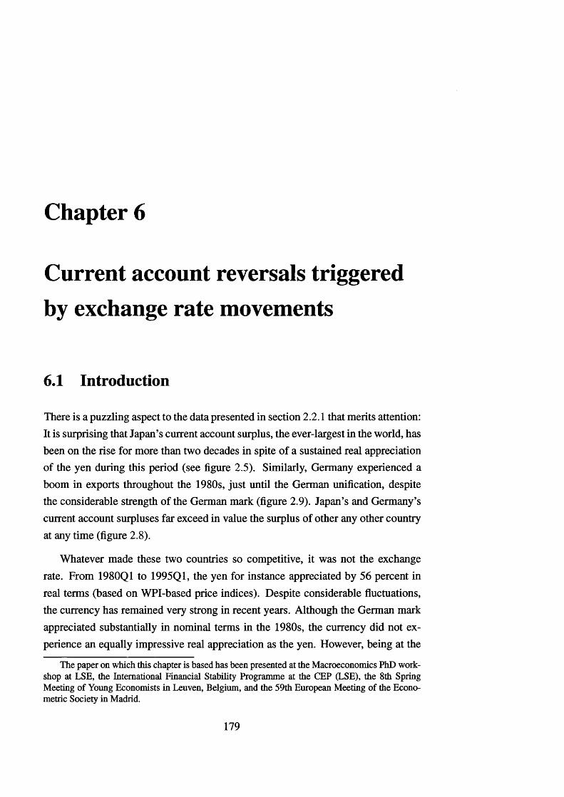
Chapter 6
Current account reversals triggered by exchange rate movements
6.1 Introduction
There is a puzzling aspect to the data presented in section 2.2.1 that merits attention: It is surprising that Japan’s current account surplus, the ever-largest in the world, has been on the rise for more than two decades in spite of a sustained real appreciation of the yen during this period (see figure 2.5). Similarly, Germany experienced a boom in exports throughout the 1980s, just until the German unification, despite the considerable strength of the German mark (figure 2.9). Japan’s and Germany’s current account surpluses far exceed in value the surplus of other any other country at any time (figure 2 .8 ).
Whatever made these two countries so competitive, it was not the exchange rate. From 1980Q1 to 1995Q1, the yen for instance appreciated by 56 percent in real terms (based on WPI-based price indices). Despite considerable fluctuations, the currency has remained very strong in recent years. Although the German mark appreciated substantially in nominal terms in the 1980s, the currency did not experience an equally impressive real appreciation as the yen. However, being at the
The paper on which this chapter is based has been presented at the Macroeconomics PhD workshop at LSE, the International Financial Stability Programme at the CEP (LSE), the 8th Spring Meeting of Young Economists in Leuven, Belgium, and the 59th European Meeting of the Econometric Society in Madrid.
179

Current account reversals triggered by exchange rate movements
time the anchor currency of the EMS, the German mark was widely perceived as a hard currency and as such not really conducive to Germany’s strong export growth.
This chapter argues that the trade performance of both countries was nevertheless affected by the exchange rate. Based on the empirical evidence, it is noted that export booms were subject to various setbacks that often lasted for several quarters or even years. Almost all of these setbacks, however, were preceded by, or occurred simultaneously with, strong exchange rate appreciations around the same period. Subsequent recoveries usually took place whenever the exchange rate had once again become more competitive.
Based on these observations, the chapter analyzes a Markov-switching time series model of the current account designed to capture the recurrent swings of this economic variable. There are two regimes, one in which the current account is heading upwards, another one in which it is declining. A crucial feature of the setup is that the transition probabilities are time-varying and in particular allowed to depend on the exchange rate.
To analyze the model, the chapter employs a Bayesian estimation strategy. For inference on the parameter posteriors and on the unobserved regimes, the simulation tool of Gibbs sampling is used. The Gibbs sampler—a method that is based on the idea of alternating conditional simulations—turns the complex conditional structure of the model to its advantage.
Of particular economic interest is the question to what extent regime changes are explained by movements of the exchange rate. To assess this question, this chapter applies the methodology of Kim and Nelson (1998), which those authors used to study the duration dependence of business cycles. The idea is to apply a variable selection procedure to a latent variable regression that determines the regime that the current account is in. The specific variable selection method adopted is that proposed by Geweke (1996) in the context of Bayesian regression.
The topic of this chapter is related to the empirical literature on the sensitivity of trade flows to exchange rate changes. A typical finding in this literature is that import and export demand elasticities are rather low and that the Marshall-Lemer condition does not hold. Some authors have called the link between the real exchange rate and the real trade balance altogether into question (see Rose, 1990).
180

Current account reversals triggered by exchange rate movements
Nevertheless, a consensus seems to exist that devaluations do improve the trade balance of countries although the effect may take a long time due to the J-curve effect.
Of interest in our context is the study of Kim (1998) who fails to detect an effect of exchange rate variations on Germany’s international competitiveness when using aggregate trade data from 1982 to 1991 (he finds, however, some effects for disaggregated data). Sawyer and Sprinkle (1997) offer a survey on this type of literature for Japan. They explicitly only consider studies that do not produce estimates with the "wrong" sign; even so, they find that imports are quite insensitive to changes in the exchange rate on average while exports appear to respond somewhat more strongly to the exchange rate.
The chapter is organized as follows. Section 6.2 examines the time series evidence of both countries. Section 6.3 introduces the empirical model. Section 6.4 reports on the data used and discusses the choice of priors. Section 6.5 presents the main empirical findings. Section 6 .6 provides conclusions.
6.2 External performance of Japan and Germany
This chapter looks at two countries that experienced remarkable export booms in the 1980s and 1990s. Consider once again figure 2.8, which gives us an idea of just how large Japan’s and Germany’s export surpluses were in US-dollar terms compared to those of other countries. Japan’s current account balance recorded the world’s ever- largest surplus during the past two decades, and it was mirrored to a large extent by the unprecedented current account deficit run by the United States. Germany also achieved a considerable surplus in the 1980s, which then turned into deficit due to the German reunification. The objective of this chapter is to understand the role that exchange rates have played in the evolution of these large external imbalances.
6.2.1 Japan
Consider figure 2.5 and 6.1, which plot the time series of Japan’s current account and of its nominal and real effective exchange rates during the 1970s, 1980s and
181

Current account reversals triggered by exchange rate movements
4.754 Current account
Nominal effective exchange rate 4.50
2 4.25
4.00
03.75
1980 1985 1990 1995
4 Current account Real effective exchange rate (WPI) 4.6
2
4.4
04.2
1980 1985 1990 1995
Figure 6.1: Japanese current account and exchange rates (1980s and 1990s). Japanese current account (left scale, in trillions of yen) and nominal and real effective exchange rates (right scale, in logarithms), period from 1977Q1 to 2001Q1. Source: International Financial Statistics (IMF).
1990s. As has been pointed out, the Japanese current account did not rise in a stable fashion but was rather subject to repeated setbacks with subsequent recoveries. Overall, the current account exhibited several large swings, all of which lasted for several years.
The other remarkable feature of the data is that all large turnarounds of the current account were preceded by large movements in the exchange rate. This is true for the export booms setting off in 1974, 1980, 1990 and 1996 with the aid of a depreciated yen. It is also true for the episodes starting in 1973, 1978, 1986 and 1993 when the current account began to weaken following large appreciations of the yen.
6.2.2 Germany
Consider now figure 6.2 which shows the corresponding time series for Germany. Apparently, the German experience is quite similar to that of Japan. Germany’s current account was also going through several upward and downward swings. And like in Japan, the temporary strength of the domestic currency, or its temporary
182

Current account reversals triggered by exchange rate movements
lOOOO 4.5rCurrent accountNominal effective exchange rate7500
4.4
5000
4.32500
JUiWlil 4.2
1980 1985 199010000 0.15
Current accountReal effective exchange rate7500 0.10
5000 0.05
2500 0.00
-0 .0 5
1980 1985 1990
Figure 6.2: German current account and nominal and real exchange rates (1980s).German current account (centered, yearly moving average, left scale, in million DM) and nominal and real effective exchange rate (monthly data, 1980s). Source: Economic Outlook (OECD), IFS (IMF).
weakness, appears to have triggered many of the turnarounds in net exports. The effect is particularly noticeable in 1978, 1981, 1983, 1984, 1986 and to a lesser extent in 1987. Note that Germany’s current account balance alternated more frequently between booms and declines than that of Japan.
6.2.3 Current account adjustment under uncertainty
Before embarking on an empirical analysis, this may be a good moment to think about the underlying economic reasons for the observed empirical regularities in both the Japanese and German data. There are in fact a number of plausible stories that can explain why it is the trend, rather than the level, of the current account that adjusts to exchange rate shifts. In both countries considered in this chapter, the current account movements were largely mirroring the performance of the trade balance in the periods considered. One possible explanation is therefore that import demands in Japan and Germany as well as in their trading partners’ economies were adjusting relatively slowly to changes in the real exchange rate. An important reason
183
55111815

Current account reversals triggered by exchange rate movements
for this could be the well-documented low rate of pass-through from exchange rate movements to import prices.
However, a potentially even more compelling economic argument would focus on the supply side rather than the demand side and be based on ideas from real options theory (see for instance Dixit and Pindyck, 1994). As noted above, the fluctuations of the current account have been rather large in Japan and Germany. Achieving higher external surpluses, and likewise reducing them, always involves considerable capacity adjustments and requires large-scale investment decisions. Since these adjustments take place under uncertainty about the movements of the exchange rate, it is difficult to predict their future payoff. At the same time, such adjustments involve large costs that may even increase with the rate at which they take place. The upshot is that firms in the export sectors need to decide not only whether and to what extent to alter their production scale but also at what time and for which horizons to take their decisions. If exchange rate movements are close to firms’ previous forecasts, little adjustment may be needed. If the exchange rate moves in unforeseen directions, however, then firms will react by changing their production capacities and carrying out the necessary investments; they may even move their production abroad, as Japanese and German car makers demonstrated during the period considered here. There are good reasons that the adjustments will be gradual rather than abrupt. First, it may pay off for firms to not to precipitate their actions but to act prudently and to wait and observe whether exchange rate movements turn out to be persistent. And as was already noticed, they may incur lower costs by carrying out changes in a smooth, rather than impatient, manner.
In summary, there are a variety of plausible explanations that can rationalize the pattern in which the current account adjusts in response to exchange rate movements. This chapter does not take a definite view on which theoretical argument has the most merit. Instead, it takes a more empirical focus as it primarily aims to characterize and examine the statistical link between exchange rate and current account movements.
184

Current account reversals triggered by exchange rate movements
6.3 Empirical framework
6.3.1 Model
In this section, a univariate Markov-switching time series model with time-varying probabilities is introduced, which makes it possible to analyze the recurrent trend reversals of the Japanese and German current account balances. The model helps to determine whether the occurrence of these reversals depends on, or is triggered by, the real exchange rate.
The current account is denoted as zt and its changes as zt, where zt = ( l - L ) Zt- The current account is modelled as an ARIMA(p, 1,0) process with a Markov- switching intercept:
Zt = ol + (3Rt + 4>iZt~\ + . . . + (f)pZt-p + £f, £ = 1,2, . . . ,T, (6.1)
where (3 > 0 and et ~ N(0, a2). R t is an unobserved random variable that takes the values 0 or 1, depending on the current account’s trend in a given period. For instance, with a < 0 and b > 0 , the current account is downward-trending if Rt = 0 and upward-trending if Rt = 1 . Suppose that regime 1 prevails whenever a latent variable, R*, is positive, such that the probability of being in regime 1 is:
Prob(Rt = 1) = Prob(tf* > 0). (6.2)
The latent variable, R*, is determined by the following equation:
Rt = 7o(l — R t- i) + j iR t- i + 6 qt + ut , (6.3)
where u t ~ N(0,1). The variable qt is a measure of real exchange rate pressure, to be discussed below. Since in this specification R*t depends on the lagged values
185

Current account reversals triggered by exchange rate movements
of Rt, the transition probabilities of Rt are time-varying and may be calculated as follows:
Prob{Rt = l\R t- i = 1) = Prob(^* > = 1)
= Prob(71 + 6 qt + u t > 0) (6.4)
= Prob(ttt > —71 — 5 qt):
Prob (Rt = 0|i^_i = 0) = Prob {R*t < 0 |^ _ i = 0)
= Prob(70 + 6 qt + u t < 0) (6.5)
= Prob(iit < - 7 0 - 6 Qt).
Note that the transition probabilities depend on qt and are therefore time- varying, except in the case in which 5 = 0 when they become constant (the case of the standard Markov-switching model). Notice also that if 5 < 0, a reversal of a current account balance that is worsening (R t = 0 ) becomes more likely when the exchange rate is weak and competitive, whereas a strong currency will sooner or later tend to bring about a turnaround when the current account balance is on the rise (Rt = 1).
6.3.2 Variable selection
To assess whether 5 is nonzero, and therefore whether the exchange rate helps to predict current account reversals, I apply the variable selection methodology proposed by Geweke (1996) in the context of Bayesian regression analysis. The method assumes that the prior distribution of S is a mixture of a—possibly truncated— normal and a discrete mass at zero. Let d be an indicator variable taking the value 1 whenever 5 is nonzero, then:
= 0 if d = 0 ,(6.6)
~N (5,u;2)i[a<*<u] i fd = 1 ,
186

Current account reversals triggered by exchange rate movements
where I[*] refers to an indicator function that serves to truncate the normal prior for (5 at A and at v. Since it is reasonable to assume here that 6 < 0, let A = — oo andv = 0 .
Now let p denote the prior probability that d is 1 and let p denote the corresponding posterior probability. Then p tells us the probability that the exchange rate is useful in explaining the probability of different regimes and should be retained in the model. Appendix 6 .B describes how p is calculated.
The issue of time-varying transition probabilities has been examined by a number of studies in the context of business cycles (see for instance Filardo and Gordon, 1998). The analysis in this chapter has been inspired by the study of Kim and Nelson (1998) who test whether during a business cycle, the probability that a boom or recession comes to an end depends on the time it has persisted already.
6.3.3 Inference
Bayesian estimation of the model proceeds via the Gibbs sampler. The details are deferred to appendix 6 .A. Appendix 6 .B describes how p can be calculated from the information delivered by the Gibbs simulations.
6.4 Data and specification of priors
6.4.1 Data
The data for Japan are taken from the International Financial Statistics of the IMF. A WPI-based real exchange rate is used in the estimations. The current account of Japan is deseasonalized using a centered, yearly moving average. The sample period of the Japanese data is from 1978Q4 to 1998Q2. The data for Germany are taken from the Economic Outlook of the OECD. The German current account is deseasonalized using a centered, 12-month moving average. The sample period of the German data is from 1979M12 to 1989M9.
187

Current account reversals triggered by exchange rate movements
6.4.2 Defining exchange rate pressure
As mentioned in the introduction, many authors belief that large movements of the real exchange rate do have impact on the trade balance but that the adjustment may take some time (see also Krugman, 1991). In assessing how the exchange rate affects their competitiveness, exporters and importers compare the most recent level of the exchange rate with the exchange rate they were adjusting to over recent years. In this model, the measure of exchange rate pressure, qt, is defined as the log of the ratio between the average real exchange rate during the previous year and the average real exchange rate during the previous three years:
Qt = Qt—ii (6.7)
where
I = <
3 for quarterly data (Japan),
11 for monthly data (Germany),
11 for quarterly data (Japan),
35 for monthly data (Germany).
The definition of qt is simple and intuitive and makes it easy to interpret the empirical results.
6.4.3 Choice of priors
In general, non-informative priors were adopted in the estimation of the model. This is true in particular for the parameter 6 , for which the prior parameterization 6 = 0 and u 2 = 106 was chosen, see equation (6 .6 ). One might want to set p, the prior probability that d = 1 , to 0.5 or even higher, given the general belief that real exchange rates matter for the current account. However, to ensure that this assumption does not drive the results, the estimations were carried out with three alternative priors for p, namely 0.25, 0.5 and 0.75.
188

Current account reversals triggered by exchange rate movements
6.5 Estimation
6.5.1 Estimation results
This section discusses the estimation results. The empirical findings for the two countries are quite similar and shall therefore be presented jointly.
Parameter
Posterior
Mean Median 90% interval
a -0.075593 -0.076182 -0.10439, -0.046257P 0.19047 0.19263 0.13692,0.237454>i 0.69158 0.68348 0.51268,0.88568<j>2 0.032266 0.035050 -0.18404,0.242814*3 -0.30266 -0.30395 -0.44706, -0.15467a 2 0.0053193 0.0051891 0.0038878, 0.00718587 i -1.2197 -1.2186 -1.8556, -0.5855872 1.5887 1.6042 0.91211,2.23516 -7.8497 -8.5782 -14.007, 0.00000
Table 6 .1: Parameter estimates for Japan. Mean, median and 90% interval of the simulated parameter posteriors.
Consider first the summary statistics for the simulated parameter posteriors of the Gibbs sampler, which are given in tables 6.1 and 6.2. Two things are worth noting: First, the parameters a and (3 are, respectively, negative and positive. The regime variable therefore distinguishes whether the current account is trending downwards or upwards. Second, 5 has the expected (negative) sign. An appreciated currency will therefore tend to force the current account to weaken, and vice versa.
Since the Gibbs sampling scheme simulates the time series of the regime variable during each iteration, it is possible to estimate the evolution of regimes by averaging over the simulations. Figures 6.3 and 6.4 depict the estimated regimes for Japan and Germany, respectively. For convenience, the time series of the current accounts of both countries (deseasonalized, as used in the estimations). In both figures, the periods of each of the two regimes, 0 and 1 , are well identified.
189

Current account reversals triggered by exchange rate movements
Parameter
Posterior
Mean Median 90% interval
a -28.814 -33.680 -76.491, 40.002P 378.55 403.33 146.69,490.36
0 i -0.25651 -0.28727 -0.45136,0.0717050 2 0.097839 0.079024 -0.061187,0.3253803 -0.23256 -0.24443 -0.39510, -0.03140404 -0.40391 -0.42418 -0.59101, -0.13973(J2 24779. 23058. 17343., 39487.7i -1.2219 -1.2669 -1.8451, -0.3849672 0.92031 1.1187 -0.84297,1.68216 -15.000 -11.806 -43.148,-1.0441
Table 6.2: Parameter estimates for Germany. Mean, median and 90% interval of the simulated parameter posteriors.
The top panels of figures 6.5 and 6 .6 plot the estimated probabilities that a particular regime will persist, that is, Prob(i?f = 0 |f?t_i = 0 ) andProb(i?f = l\R t-i = 1). The transition probabilities for the regimes are easily calculated as one minus the plotted probabilities. Note that if S was zero, the transition probabilities would be constant. However, the estimated transition probabilities in figures 6.5 and 6 .6
are clearly time-varying. This is due to the fact that the exchange rate does play a role in determining the trends and occasional reversals of the current account in both countries.
The lower panels of figures 6.5 and 6 .6 plot for each period the expected regime duration that would result if the transition probability prevailing in the particular period would remain at its present level. The graphs suggest that when the exchange rate is favourable to the prevailing trend of the current account, the trend may be expected to last very long, provided the exchange rate remains unaltered.
6.5.2 Significance of the exchange rate
Table 6.3 presents the posterior estimates of p, the probability that d = 1, under different assumptions about the prior probability, p. Both for Japan and Germany, there appears to be strong evidence in favour of including qt, the measure of exchange rate pressure, into the latent variable regression in equation (6.3).
190

Current account reversals triggered by exchange rate movements
1.00
0.75
0.50
0.25
C u rren t a cco u n t
1980 1985
P ro b [R (t)= l |.] (m ean )
1990 1995
1 1 i1980 1985 1990 1995
Figure 6.3: Regime probabilities (Japan). Top: Japanese current account (deseasonalized). Bottom: mean posterior probabilities of the Japanese current account in regime 1, Prob (Rt = 1).
Japan: Prob(di = 1) Germany: Probfdi = 1)
Prior: p2 Posterior: P2 Prior: p2 Posterior: p2
0.25 0.84840 0.25 0.951200.5 0.86760 0.5 0.96040
0.75 0.87920 0.75 0.96760
Table 6.3: Posterior probabilities that d\ = 1 (Japan and Germany). Posterior probabilities p that d = 1, using different priors, p , for Japanese and German data.
6.6 Conclusions
This chapter applies a Markov-switching time series model with time-varying probabilities to the current account balances of Japan and Germany. The current account is subject to occasional trend reversals whose probability is assumed to depend, among other things, on the level of the exchange rate. It is shown that Bayesian inference is feasible via a Gibbs sampling scheme. A variable selection procedure is used to investigate whether the real exchange rate helps to explain the occurrence of current account reversals.
191
^99999999999999999
9999994

Current account reversals triggered by exchange rate movements
lOOOO
7500
5000
2500
0
1.00
0.75
0.50
0.25
C u rre n t a cco u n t
IP.•■II
1981 1982 1983
P ro b [R (t)= l |.] (m ean )
1984 1985 1986 1987 1988 1989
1981 1982 1983 1984 1985 1986 1987 1988 1989
Figure 6.4: Regime probabilities (Germany) Top: German current account (deseasonalized, in millions of German mark). Bottom: mean posterior probabilities of the German current account in being regime 1, that is, Prob(-R* = 1).
The chapter finds strong evidence of recurrent current account reversals, both in Japan and Germany. For each period, it presents posterior estimates of the probability that the current account is in a particular regime (boom or decline) as well as of the time-varying probability that the current account will stay in that regime. The hypothesis that the real exchange rate can explain the occurrence of current account reversals is also supported by data. This result is robust to assumptions about priors and other aspects of the model.
This chapter offers a novel perspective regarding the impact of the exchange rate on the current account. Underlying the empirical model in this chapter is the idea that exchange rate movements can lead to a trend reversals of the current account in situations when they move too far away from their trend. In comparison, marginal changes in the exchange rate induce only minor adjustments. The chapter’s message therefore is that exchange rates only hurt when they move too strongly into the wrong direction.
The chapter may thus help to explain why empirical researchers have found it difficult to come up with reasonably large—or indeed correctly-signed—estimates for the sensitivity of trade flows to exchange rate movements. An interesting aspect
192
3360

Current account reversals triggered by exchange rate movements
Prob[R(t)=0|R(t—1)=0] (mean, for quarters)
1980 1985 1990 1995
■ Prob[R( t)= 1 |R(t— 1 )= 1 ] (mean, for quarters)
1980 1985 1990 1995
Expected duration lof regime 0 (in quarters)
20
10
1980 1985 1990 1995
30 Expected duration of regime 1 in quarters)
20
10
1980 1985 1990 1995
Figure 6.5: Time-varying transition probabilities (Japan). Top panel: transition probabilities, Prob[i?t = 0|.R£_i = 0] and Prob[i2< = l \R t-i = 1], for Japan (for quarterly data). Bottom panel: expected duration of regime 0 and 1 (in quarters), computed from the transition probability in each period, on the assumption that the determinants of the transition probability remain unchanged.
of the setup used here is that even though the current account and the exchange rate are not independent, neither the level of the current account nor its changes need to be correlated with the exchange rate at all.
Further theoretical research would be desirable to better understand the apparent persistence of current account reversals that are set into motion by exchange rate fluctuations. Another interesting topic for future research is the possibility of a dynamic feedback from the current account to the exchange rate, for which there seems to be evidence both in the Japanese and German data (Muller-Plantenberg, 2003c).
193
28

Current account reversals triggered by exchange rate movements
Expected duration of regime
1980 1985 1990 1980 1985 1990
1990
1.00
0.75
0.50
0.25
1980 1985
- Expected duration o f regime 0 (in
Prob[R(t)=l|R(t—1)=1] (mean, for quarters)
1.00
0.75
0.50
0.25
Prob[R(t)=0|R(t—1)=0] (mean, for quarters)
10.0
7.5
5.0
2.5
0.0
1985
1 (in quarters)
Figure 6.6: Time-varying transition probabilities (Germany). Top panel: transitionprobabilities, Prob[i?t = 0|i?*_i = 0] and Probji^ = l \R t- i = 1], for Germany; calculated for quarters rather than months to facilitate comparison with the corresponding probabilities for Japan. Bottom panel: expected duration of regime 0 and 1 (in quarters), computed from the transition probability of each period, on the assumption that the determinants of the transition probability remain unchanged.
Appendix 6.A Bayesian estimation
6.A.1 Gibbs sampling
To carry out Bayesian inference on the model, the simulation tool of Gibbs sampling is used. For an introduction to MCMC methods and the Gibbs sampler, see for example Gelman et al. (1995) and Kim and Nelson (1999).
The objective is to find a complete set of conditional distributions of all the parameters, on which the Gibbs sampling scheme can be run. It turns out that this task is facilitated once we treat the regimes, {R\, R 2, . . . , R t }, as well as the latent regimes, {R*y R %,. . . , }, as additional unknown parameters and analyze themjointly with other parameters (Albert and Chib, 1993). Given the regimes and latent regimes, conditional inference on all other parameters amounts to the estimation of the parameters of two independent regression equations. Given the parameters,
194
3460
2699999999999^

Current account reversals triggered by exchange rate movements
however, procedures are available that enable us to retrieve the conditional distribution of {Ri, R2, . • •, Rt } and {R\, R%, • • ■, Rt }-
6.A.2 Conditional structure of the model
For use below, define z = [z\, z2, . . . , z t ]', R t = [Ri, R 2 , • • •, Rt]' and R ^ = [Ri, R%,. . . , R j]f and let (j>= [(j>i,<j)2 , . . . ,4>p\f. To allow for general applicability, it is from now on assumed that, apart from the lagged regimes, there are m variables in the latent regime equation (6.3), denoted q u ,i= 1,2, . . . , m. Define the T x m data matrix qr = [#«]'.
The conditional distributions that form the basis of the simulation are given by:
• a, P | zT, Rt , <t>, o1
• a2 | zT, Rt , ol, P, <p
• (j) | z r , R T,a,P,(T2
• Rt | R_t, zt, R*t , a, /?, (j), a2, 7 1 , 7 2 , £*, t = 1,2 , . . . , T
• | RT,h , lU l2 ,& i
• 7i> 72 |
• ̂ | Rqi, % T , l \ , l2 ,
where R - t = [-Ri, R2 , • • •, i2t-i} #t+i>. . . , it/r]'- Each of these complete conditionals can be simulated, thus leading, via the Gibbs sampler, to a posterior sample from the joint distribution of the parameters, the regimes and the latent regimes.
The Gibbs sampler converges rapidly and is run with 4500 iterations, the initial half of which are discarded.
195

Current account reversals triggered by exchange rate movements
6.A.3 Simulation of parameters and regimes
Generating a and p The parameters a and (3 are generated conditional on zt, Rt , 4>, cr2. Consider the following regression:
<f>(L)zt = ot + (3Rt + Et, t= 1,2, . . . ,T,
where </>(L) = 1 — .. .—(f)pLP. Define the matrices Y\ and X \ as the matrices of the left-hand-side and th£ right-hand-side variables of this regression, respectively. Let 6 = [a, (3]', and let us adopt a normally distributed prior, 9 ~ N(0,0 ), where © is a diagonal matrix. The posterior is then given by:
6\zT,R T,<t>,<T2 ~ N(0,0),
where 0 = (O’ 1 + a~2 X i X x) - x and 0 = B{& -x0 + a ^ x p i ) .
Generating a 2 To generate a2 conditional on z t , R t, & and P, the following prior is employed:
~ i g ( 7 ’ j )-
where IG refers to the inverted Gamma distribution and i>\ and z>2 are appropriately chosen (here i>\ and z>2 are both set to zero, implying a non-informative prior). The posterior is then given by:
a 2 fzT,R T, a , l 3 ~ l G ( ^ , ^ ) ,
where = v\ + T and z>2 = z>2 + (Yi — Xi0y(Yi — X\9).
Generating <j> The parameters </>i, . . . , (j)p are generated conditional on zt, Rt ,P, a2. Consider the following regression:
— a — PRt = (piZt-\ + . . . + (ppZf—p + £t, t = 1,2, . . . , T.
196

Current account reversals triggered by exchange rate movements
Define the matrices Y2 and X 2 as the matrices of the left-hand-side and the right-hand-side variables of this regression, respectively. Let us adopt a normally distributed prior, 0 ~ i ) , where is a diagonal matrix. The posterior is thengiven by:
<f> ~ N(0, $)i[a(0 )],
where $ = (4 " 1 + o - 2X2 'x 2) " \ 4> = + <t~2 X'2 Y2) and I[s(<£)] is an
Generating R t The regimes Rt, t = 1,2, . . . , T, are generated one at a time, where use is made of the single-move Gibbs sampling procedure suggested by Albert and Chib (1993).
Generating R? Once simulated values of Rt are obtained, it is straightforward to generate R%, t = 1,2 , . . . , T, from equation (6.3):
Note that the simulation of enables us to analyze the conditional distributions of the parameters of equation (6.3). By artificially generating data for the latent variable, we are applying the idea of data augmentation as originally proposed by Tanner and Wong (1987).
Generating 7 The parameters 70 and 71 are generated conditional on R y, c\t and S{. Consider the following regression:
Rt ~ $iQt = 7o(l — R t-1) + IfiRt-i + ut .
Define the matrices Y3 and X 3 as the matrices of the left-hand-side and the right-hand-side variables of this regression, respectively. Let 7 = [70,71]', and let
indicator function used to denote that the roots of (j>(L) lie outside the unit circle.
N(7o(1 — R t-1) + j iR t- i + ^2i Si qit, l)i(i^>o) if Rt — 1)
N(7 o(1 — R t-1) + 7 1 -ftt-i + Qit-> l)i(#j<o) if Rt — 0-
197

Current account reversals triggered by exchange rate movements
us adopt a normally distributed prior, 7 ~ N(7 , f ) , where f is a diagonal matrix. The posterior is then given by:
7 | i $ ,S r , * i ~ N ( 7 , r ) ,
where f = ( f " 1 + X s '^ s ) - 1 and 7 = r t f - 1'/ + X'z%).
Generating Si For each ie{l, 2 , . . . , ra}, = 0 if = 0. If di / 0, the generationof 5^ conditional on qr, 7 0 , Sj#, proceeds as follows. Consider the regression:
Rt 7o(l Rt—1) 7i-^t—1 ^ ̂ Qit “1“ Ut-
Define the matrices V4 and X 4 as the matrices of the left-hand-side and the right-hand-side variables of this regression, respectively. Consider the prior
Si ~ ^{Si^i^lXiCSiKVi],
where I[ ] refers to an indicator function allowing for the possibility of a truncated normal prior. The posterior is then given by:
&i\Rri Qt 5 7» ^ N($t, )i[Ai<5i<i>i]?
where a;? = {6j12+ X 4X 4)~1 and^ = (u~25i+X4Y4). Notice that the truncationof the prior carries over to the posterior.
Appendix 6.B Variable selection in latent regime equation
This section describes how the variable selection procedure of Geweke (1996) is employed in this chapter. Recall that in equation (6.3), a variable qit ic {1 , 2 , . . . , m}, is retained if and only if di — 1 ; otherwise it is excluded from the model. This suggests carrying out the following procedure during each iteration
198

Current account reversals triggered by exchange rate movements
of the Gibbs sampler, consecutively for each z e {1 , 2 , . . . , m}: First, evaluate pit the conditional posterior probability that di = 1. Then, based on a comparison of pi with a drawing from the uniform distribution, set di to 1 or 0 .
Let BFi denote the conditional Bayes factor in favour of di = 1 versus di = 0, conditional on the other parameters of the model, and recall that pi is the prior probability that di = 1. As shown in Geweke (1996), pi can be calculated as follows:
The conditional Bayes factor in favour of di = 1 versus di = 0 is given by:
— XT It ---------
Pt (I - pi) + pi xB F 'pi x BF
BF
where <£(•) denotes the cdf of the normal distribution.
199

Chapter references
Albert, J. H. and Chib, S. (1993), ‘Bayes inference via Gibbs sampling of autoregressive time series subject to markov mean and variance shifts’, Journal of Business and Economic Statistics 11(1), 1-15.
Dixit, A. K. and Pindyck, R. S. (1994), Investment under Uncertainty, Princeton University Press, Princeton, New Jersey.
Filardo, A. J. and Gordon, D. B. (1998), ‘Business cycle durations’, Journal of Econometrics 85, 99-123.
Gelman, A., Carlin, J. B., Stem, H. S. and Rubin, D. B. (1995), Bayesian Data Analysis, Chapman and Hall, London.
Geweke, J. (1996), Variable selection and model comparison in regression, in J. O. Berger, J. M. Bernardo, A. P. Dawid, A. F. M. Smith et al., eds, ‘Proceedings on the Fifth Valencia International Meeting on Bayesian Statistics’, Oxford University Press, Oxford.
Kim, C.-J. and Nelson, C. R. (1998), ‘Business cycle turning points, a new coincident index, and tests of duration dependence based on a dynamic factor model with regime-switching’, Review of Economics and Economic Statistics pp. 188-201.
Kim, C.-J. and Nelson, C. R. (1999), State-Space Models with Regime Switching: Classical and Gibbs-Sampling Approaches with Applications, MIT Press, Cambridge, Mass.
200

Chapter references
Kim, C. K. (1998), ‘Exchange rate variations and the trade structure in the Federal Republic of Germany’, JahrbUcher fur Nationaldkonomie und Statistik 217(2), 161-184.
Krugman, R R. (1991), Has the adjustment process worked?, in C. F. Bergsten, ed., ‘International Adjustment and Financing’, Institute for International Economics, Washington, DC.
Miiller-Plantenberg, N. (2003), Long swings in Japan's current account and in the yen. Unpublished working paper, London School of Economics.
Rose, A. K. (1990), ‘Exchange rates and the trade balance: Some evidence from developing countries’, Economics Letters 34(3), 271-275.
Sawyer, W. C. and Sprinkle, R. L. (1997), ‘The demand for imports and exports in Japan: a survey’, Journal of the Japanese and International Economies 11(2), 247-259.
Tanner, M. A. and Wong, W. H. (1987), ‘The calculation of posterior densities by data augmentation’, Journal o f the American Statistical Association 82(398), 528-540.
201

Bibliography
Abel, A. B. and Bemanke, B. S. (2003), Macroeconomics, Addison Wesley, Boston, London.
Adda, J. and Cooper, R. (2003), Dynamic Economics: Quantitative Methods and Applications, MIT Press, Cambridge, Mass.
Agenor, P.-R. and Montiel, P. J. (1999), Development macroeconomics, Princeton University Press, Princeton, New Jersey.
Albert, J. H. and Chib, S. (1993), ‘Bayes inference via Gibbs sampling of autoregressive time series subject to markov mean and variance shifts’, Journal of Business and Economic Statistics 11(1), 1-15.
Appleyard, D. R. and Field, A. J. (2001), International Economics, McGraw-Hill, Boston.
Balassa, B. (1964), ‘The purchasing power parity doctrine: A reappraisal’, Journal of Political Economy 72(6), 584-596.
Bauwens, L., Lubrano, M. and Richard, J.-F. (1999), Bayesian Inference and Dynamic Econometric Models, Oxford University Press, New York.
Bauwens, L. and Richard, J.-F. (1985), ‘A 1-1 poly-t random variable generator with application to Monte Carlo integration’, Journal of Econometrics 29,19^16.
Blanchard, O. J. (2003), Macroeconomics, Prentice-Hall International, Upper Saddle River, New Jersey.
Blanchard, O. J. and Fischer, S. (1989), Lectures on Macroeconomics, MIT Press, Cambridge, Mass.
202

Bibliography
Brooks, R., Edison, H. J., Kumar, M. and Sl0 k, T. (2001), ‘Exchange rates and capital flows’, International Monetary Fund Working Papers (190).
Burda, M. and Wyplosz, C. (2001), Macroeconomics: a European text, Oxford University Press, Oxford.
Bussiere, M. and Mulder, C. (1999), ‘External vulnerability in emerging market economies: How high liquidity can offset weak fundamentals and the effects of contagion’, International Monetary Fund Working Papers (8 8 ).
Calvo, G. A., Leiderman, L. and Reinhart, C. M. (1996), ‘Inflows of capital to developing countries in the 1990s’, Journal o f Economic Perspectives 10,123- 139.
Chen, Y.-c. and Rogoff, K. (2003), ‘Commodity currencies’, Journal o f International Economics 60, 133-160.
Cheung, Y.-W., Chinn, M. D. and Garcia Pascual, A. (n.d.), Empirical exchange rate models of the ninetees: Are any fit to survive? Forthcoming.
Cheung, Y.-W. and Wong, C. Y.-P. (2000), ‘A survey of market practitioners" views on exchange rate dynamics’, Journal o f International Economics 51(2), 401- 420.
Copeland, L. (2004), Exchange Rates and International Finance, FT Prentice Hall, Harlow.
Das, D. K. (1993), The internationalization of the yen, in D. K. Das, ed., ‘International Finance: Contemporary Issues’, Routledge, London and New York, pp. 580-591.
Dixit, A. K. and Pindyck, R. S. (1994), Investment under Uncertainty, Princeton University Press, Princeton, New Jersey.
Doomik, J. A. and Henry, D. F. (1997), Modelling Dynamic Systems Using PcFiml 9.0 for Windows, International Thomson Business Press, London, Boston.
Doomik, J. A. and Ooms, M. (2001), ‘Introduction to Ox: Ox version 3’.
203

Bibliography
Eichengreen, B. (1990), ‘Trends and cycles in foreign lending’, National Bureau of Economic Research Working Papers (3411).
Eichengreen, B. (1996), Globalizing Capital, Princeton University Press, Princeton, New Jersey.
Eichengreen, B. (2003), Capital Flows and Crises, The MIT Press, Cambridge, Massachusetts; London.
Eichengreen, B., Rose, A. K. and Wyplosz, C. (1995), ‘Exchange market mayhem: The antecedents and aftermaths of speculative attacks’, Economic Policy 21, 249-312.
Engel, C. (1999), ‘Accounting for US real exchange rate changes’, Journal of Political Economy 107(3), 507-538.
Engel, C. and Hamilton, J. D. (1990), ‘Long swings in the dollar: Are they in the data and do markets know it?’, American Economic Review 80(4), 689-713.
Engel, C. and West, K. D. (2004), ‘Exchange rates and fundamentals’, National Bureau o f Economic Research Working Papers (10723).
Evans, C. L. and Lyons, R. K. (2002), ‘Order flow and exchange rate dynamics’, Journal o f Political Economy 110(1), 170-180.
Evans, M. D. D. and Lyons, R. K. (2003), ‘New micro exchange rate economics’. Unpublished working paper, Haas School of Business, UC Berkeley.
Feldstein, M. S. and Horioka, C. (1980), ‘Domestic savings and international capital flows’, Economic Journal (90), 314-329.
Filardo, A. J. and Gordon, D. B. (1998), ‘Business cycle durations’, Journal of Econometrics 85, 99-123.
Fischer, S. (2001), ‘Exchange rate regimes: Is the bipolar view correct?’, Journal of Economic Perspectives 15(2), 3-24.
Rood, R. P. and Garber, P. M. (1984), ‘Collapsing exchange-rate regimes: some linear examples’, Journal of International Economics 17(0), 1-13.
204

Bibliography
Frankel, J. A. (1984), ‘The yen/dollar agreement: Liberalizing Japanese capital markets’, Policy Analyses in International Economics (Institute for International Economics) (9).
Frankel, J. A. (1985), ‘The dazzling dollar’, Brookings Papers on Economic Activity (1), 199-217.
Frankel, J. A. and Rose, A. K. (1995), An empirical characterization of nominal exchange rates, in Grossman and Rogoff (1995), pp. 1689-1729.
Garcia, R. and Perron, P. (1996), ‘An analysis of real interest under regime shift’, Review of Economics and Statistics 78(1), 111-125.
Gelman, A., Carlin, J. B., Stem, H. S. and Rubin, D. B. (1995), Bayesian Data Analysis, Chapman and Hall, London.
Geweke, J. (1996), Variable selection and model comparison in regression, in J. O. Berger, J. M. Bernardo, A. P. Dawid, A. F. M. Smith et al., eds, ‘Proceedings on the Fifth Valencia International Meeting on Bayesian Statistics’, Oxford University Press, Oxford.
Girton, L. and Roper, D. (1977), ‘A monetary model of exchange market pressure applied to the postwar Canadian experience’, American Economic Review 67(4), 537-548.
Grenville, S. A. (1998), ‘Capital flows and crises’, Reserve Bank o f Australia Bulletin .
Grossman, G. M. and Rogoff, K., eds (1995), Handbook o f International Economics, Vol. 3, North Holland, Amsterdam.
Hailwood, P. and MacDonald, R. (2000), International Money and Finance, Black- well, Malden, MA.
Hamilton, J. D. (1989), ‘A new approach to the economic analysis of nonstationary time series and the business cycle’, Econometrica 57(2), 357-384.
Hau, H. and Rey, H. (2003), ‘Exchange rates, equity prices and capital flows’, Centre for Economic Policy Research Discussion Papers (3735).
205

Bibliography
Heijdra, B. J. and van der Ploeg, F. (2002), Foundations o f Modem Macroeconomics, Oxford University Press, Oxford, New York.
Hooper, P. and Morten, J. E. (1982), ‘Fluctuations in the dollar: a model of nominal and real exchange rate fluctuations’, Journal o f International Money and Finance 1, 39-56.
Imbs, J., Mumtaz, H., Ravn, M. O. and Rey, H. (2002), ‘PPP strikes back: Aggregation and the real exchange rate’, National Bureau of Economic Research Working Papers (9372).
Isard, P. and Stekler, L. (1985), ‘U.S. international capital flows and the dollar’, Brookings Papers on Economic Activity (1), 219-236.
Johansen, S. (1988), ‘Statistical analysis of cointegration vectors’, Journal of Economic Dynamics and Control 12, 231-254.
Kenen, P. B. (2000), The International Economy, Cambridge University Press, Cambridge (United Kingdom), New York.
Keynes, J. M. (1929), ‘The German transfer problem’, The Economic Journal 39(153), 1-7.
Kim, C.-J. and Nelson, C. R. (1998), ‘Business cycle turning points, a new coincident index, and tests of duration dependence based on a dynamic factor model with regime-switching’, Review of Economics and Economic Statisticspp. 188-201.
Kim, C.-J. and Nelson, C. R. (1999), State-Space Models with Regime Switching: Classical and Gibbs-Sampling Approaches with Applications, MIT Press, Cambridge, Mass.
Kim, C. K. (1998), ‘Exchange rate variations and the trade structure in the Federal Republic of Germany’, JahrbUcher fur Nationalokonomie und Statistik 217(2), 161-184.
Kouri, P. J. K. (1976), ‘The exchange rate and the balance of payments in the short run and in the long run: A monetary approach’, Scandinavian Journal o f Economics 78, 280-304.
206

Bibliography
Kraay, A., Loayza, N., Serven, L. and Ventura, J. (2000), ‘Country portfolios’, National Bureau of Economic Research Working Papers (7795).
Kreyszig, E. (1999), Advanced Engineering Mathematics, John Wiley and Sons, New York.
Krugman, P. R. (1979), ‘A model of balance-of-payments crises’, Journal o f Money, Credit, and Banking 11(3), 311-325.
Krugman, P. R. (1985), Is the strong dollar sustainable?, in Federal Reserve Bank of Kansas City, ed., ‘The U.S. Dollar: Recent Developments, Outlook, and Policy Options’, pp. 103-132.
Krugman, P. R. (1991), Has the adjustment process worked?, in C. F. Bergsten, ed., ‘International Adjustment and Financing’, Institute for International Economics, Washington, DC.
Krugman, P. R. (1999), ‘Balance sheets, the transfer problem, and financial crises’, International Tax and Public Finance 6,459-472.
Krugman, P. R. and Obstfeld, M. (2003), International Economics, Addison Wesley, Boston.
Lane, P. R. and Milesi-Ferretti, G. M. (2000), ‘The transfer problem revisited: Real exchange rates and net foreign assets’, Centre for Economic Policy Research Discussion Papers (2511).
Ljungqvist, L. and Sargent, T. J. (2004), Recursive Macroeconomic Theory, MIT Press, Cambridge, Massachusetts; London.
Lyons, R. K. (2001), The Microstructure Approach to Exchange Rates. Forthcoming, Fall 2001, MIT Press.
MacDonald, R. (1999a), ‘Exchange rate behaviour: Are fundamentals important?’, The Economic Journal 109, 673-691.
MacDonald, R. (1999b), What do we really know about real exchange rates?, in R. MacDonald and J. L. Stein, eds, ‘Equilibrium Exchange Rates’, Kluwer Academic Publishers, Boston, Dordrecht and London, pp. 19-65.
207

Bibliography
Machlup, F. (1939), ‘The theory of foreign exchanges’, Economica 6(24), 375-397.
Machlup, F. (1940), ‘The theory of foreign exchanges’, Economica 7(25), 23-49.
Mankiw, N. G. (2002), Macroeconomics, Worth Publishers, New York.
McKinnon, R. I. and Pill, H. (1997), ‘Credible economic liberalizations and over- borrowing’, American Economic Review 87(2), 189-193.
Meese, R. and Rogoff, K. (1983a), ‘Empirical exchange rate models of the seventies: Do they fit out of sample?’, Journal o f International Economics 14,3-24.
Meese, R. and Rogoff, K. (1983b \ The out-of-sample failure of empirical exchange rate models, in J. A. Frenkel, ed., ‘Exchange Rates and International Macroeconomics’, Chicago University Press, Chicago.
Michael, P., Nobay, A. R. and Peel, D. A. (1997), ‘Transaction costs and nonlinear adjustment in real exchange rates: an empirical investigation’, Journal of Political Economy 105(4), 862-879.
Miiller-Plantenberg, N. (2003a), Current account reversals triggered by large exchange rate movements. Unpublished working paper, London School of Economics.
Miiller-Plantenberg, N. (2003b), ‘Japan’s imbalance of payments’, CESifo Working Paper Series (1089). Forthcoming in: Michael Hutchison and Frank Wester- mann (eds.), Economic Stagnation in Japan, MIT Press.
Miiller-Plantenberg, N. (2003c), Long swings in Japan's current account and in the yen. Unpublished working paper, London School of Economics.
Montiel, P. J. and Reinhart, C. M. (2001), The dynamics of capital movements to emerging economies during the 1990s, in S. Griffith-Jones, M. F. Montes and A. Nasution, eds, ‘Short-Term Capital Movements and Economic Crises’, Oxford University Press, Oxford.
Mussa, M. (1979), ‘Empirical regularities in the behavior of exchange rates and theories of the foreign exchange market’, Camegie-Rochester Conference Series on Public Policy 11, 9-57.
208

Bibliography
Obstfeld, M. (1986), ‘Rational and self-fulfilling balance-of-payments crises’, American Economic Review 76(1), 72-81.
Obstfeld, M. (1994), ‘The logic of currency crises’, Cahiers Economiques et Mon- etaires (43).
Obstfeld, M. and Rogoff, K. (1995), The intertemporal approach to the current account, in Grossman and Rogoff (1995), pp. 1731-1799.
Obstfeld, M. and Rogoff, K. (1996), Foundations o f International Macroeconomics, MIT Press, Cambridge, Massachusetts.
Obstfeld, M. and Rogoff, K. (2000a), Perspectives on OECD economic integration: Implications for US current account adjustment.
Obstfeld, M. and Rogoff, K. (2000&), The six major puzzles in international macroeconomics: Is there a common cause?, in B. S. Bemanke and K. Rogoff, eds, ‘NBER Macroeconomics Annual’, Vol. 15, MIT Press.
Obstfeld, M. and Rogoff, K. (2004), ‘The unsustainable US current account position revisited’, National Bureau o f Economic Research Working Papers (10869).
Obstfeld, M. and Taylor, A. M. (1997), ‘Nonlinear aspects of goods-market arbitrage and adjustment: Heckscher's commodity points revisited’, Journal of the Japanese and International Economies 11,441-479.
Ritter, C. and Tanner, M. A. (1992), ‘Facilitating the Gibbs sampler: the Gibbs stopper and the griddy-Gibbs sampler’, Journal o f the American Statistical Association 87(419), 861-868.
Robinson, J. (1937a), ‘Essays in the theory of employment’.
Robinson, J. (1937&), The foreign exchanges, in Essays in the Theory of Employment (Robinson, 1937a).
Rogoff, K. (1996), ‘The purchasing power parity puzzle’, Journal of Economic Literature 34, 647-668.
Rogoff, K. (2002), ‘The failure of empirical exchange rate models: No longer new, but still true’, Economic Policy Web Essays .
209

Bibliography
Romer, D. (1996), Advanced Macroeconomics, McGraw-Hill.
Rose, A. K. (1990), ‘Exchange rates and the trade balance: Some evidence from developing countries’, Economics Letters 34(3), 271-275.
Rosenberg, M. R. (1996), Currency Forecasting. A Guide to Fundamental and Technical Models o f Exchange Rate Determination, Irwin, London, Chicago, Singapore.
Sachs, J. D., Tomell, A. and Velasco, A. (1996), ‘The Mexican peso crisis: Sudden death or death foretold?’, Journal of International Economics 41, 265-283.
Salant, S. W. and Henderson, D. W. (1978), ‘Market anticipations of government policies and the price of gold’, Journal o f Political Economy 86(4), 627-648.
Samuelson, R A. (1964), ‘Theoretical notes on trade problems’, Review of Economics and Statistics 46, 145-154.
Sargent, T. J. (1987tf), Dynamic Macroeconomic Theory, Harvard University Press, Cambridge, Mass., London.
Sargent, T. J. (1987&), Macroeconomic Theory, Academic Press, New York.
Samo, L. and Taylor, M. P. (2002), The Economics o f Exchange Rates, Cambridge University Press, Cambridge.
Sawyer, W. C. and Sprinkle, R. L. (1997), ‘The demand for imports and exports in Japan: a survey’, Journal of the Japanese and International Economies 11(2), 247-259.
Stroud, K. A. and Booth, D. J. (2003), Advanced Engineering Mathematics, Pal- grave Macmillan, Hampshire and New York.
Svensson, L. E. O. (2001), ‘The zero bound in an open economy: A foolproof way of escaping from a liquidity trap’, Monetary and Economic Studies (Bank of Japan J 19, 277-312.
Tanner, M. A. and Wong, W. H. (1987), ‘The calculation of posterior densities by data augmentation’, Journal of the American Statistical Association 82(398), 528-540.
210

Bibliography
Taylor, A. M. (2002), ‘A century of current accout dynamics’, Journal of International Money and Finance 21, 725-748.
Taylor, M. P. (1995), ‘The economics of exchange rates’, Journal of Economic Literature 33(1), 13-47.
Taylor, M. P. and Peel, D. A. (2000), ‘Nonlinear adjustment, long-run equilibrium and exchange rate fundamentals’, Journal o f International Money and Finance 19, 33-53.
Tesar, L. L. and Werner, I. M. (1995), ‘Home bias and high turnover’, Journal o f International Money and Finance 14(4), 467-492.
Tumovsky, S. (2000), Methods o f Macroeconomic Dynamics, MIT Press, Cambridge, Massachusetts.
Wang, Y. (2002), ‘Capital account liberalization: The case of Korea’.
Williamson, J. (1985), The Exchange Rate System, Institute for International Economics, Washington, DC.
211