Anatoli PolkovnikovBoston University

L. D’Alessio BU M. Bukov BUC. De Grandi Yale V. Gritsev AmsterdamM. Kolodrubetz Berkeley C.-W. Liu BUP. Mehta BU M. Tomka BUD. Sels BU A. Sandvik BUT. Souza BU

Designer quantum systems out of equilibrium, KITP, 11/16/2016

Outline

1. Motion in a moving frame and non-adiabatic response (inertia, Coriolis force, …).

2. Counter-diabatic driving and quantum speed limit.

3. Variational approach for gauge potentials (connection operators). Application to many-particle systems

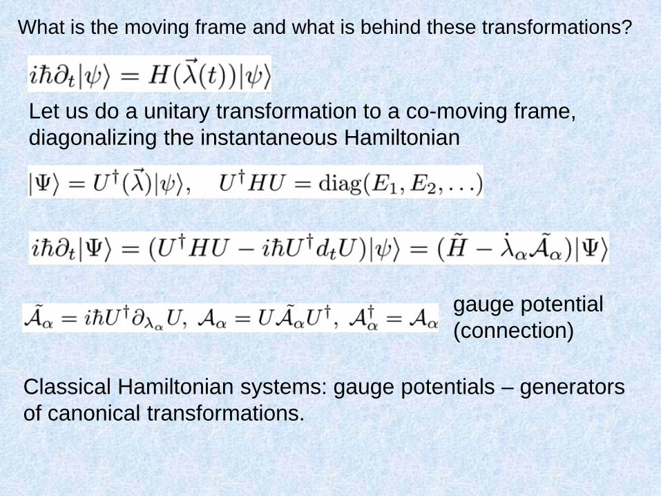
What is the moving frame and what is behind these transformations?

Let us do a unitary transformation to a co-moving frame, diagonalizing the instantaneous Hamiltonian

gauge potential (connection)

Classical Hamiltonian systems: gauge potentials – generators of canonical transformations.

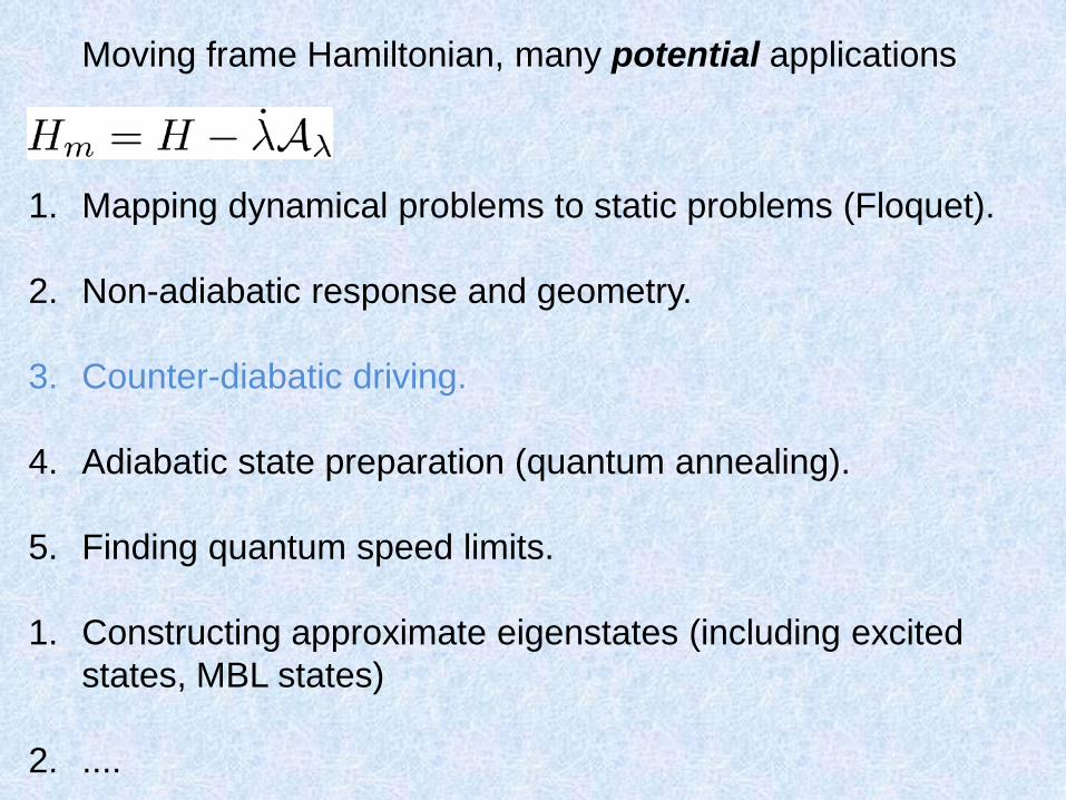
Moving frame Hamiltonian, many potential applications

1. Mapping dynamical problems to static problems (Floquet).

2. Non-adiabatic response and geometry.

3. Counter-diabatic driving.

4. Adiabatic state preparation (quantum annealing).

5. Finding quantum speed limits.

1. Constructing approximate eigenstates (including excited states, MBL states)

2. ....

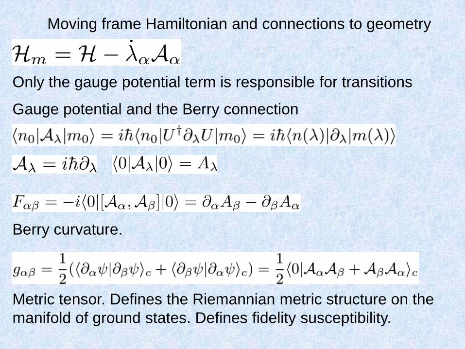
Moving frame Hamiltonian and connections to geometry

Only the gauge potential term is responsible for transitions

Gauge potential and the Berry connection

Berry curvature.

Metric tensor. Defines the Riemannian metric structure on the manifold of ground states. Defines fidelity susceptibility.

Compute leading correction to the energy due to the Galilean term (consider the ground state)

Recover the mass term as the leading non-adiabatic correction to the energy. Inertia appears as noni-adiabatic response.

F

Galilean Transformation

Can recover many familiar results from non-adiabatic perturbation theory

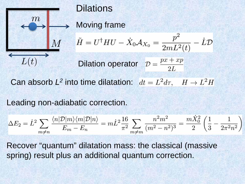
Dilation operator

Recover “quantum” dilatation mass: the classical (massive spring) result plus an additional quantum correction.

Leading non-adiabatic correction.

Moving frame

Can absorb L2 into time dilatation:

Dilations

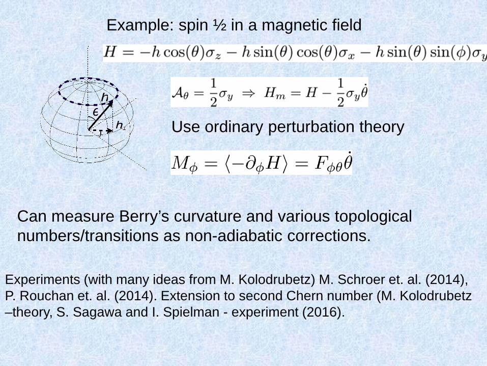
Example: spin ½ in a magnetic field

Use ordinary perturbation theory

Can measure Berry’s curvature and various topological numbers/transitions as non-adiabatic corrections.

Experiments (with many ideas from M. Kolodrubetz) M. Schroer et. al. (2014), P. Rouchan et. al. (2014). Extension to second Chern number (M. Kolodrubetz–theory, S. Sagawa and I. Spielman - experiment (2016).

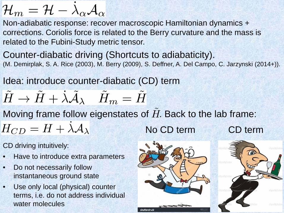
Counter-diabatic driving (Shortcuts to adiabaticity).(M. Demirplak, S. A. Rice (2003), M. Berry (2009), S. Deffner, A. Del Campo, C. Jarzynski (2014+)).

Idea: introduce counter-diabatic (CD) term

Moving frame follow eigenstates of . Back to the lab frame: No CD term CD term

CD driving intuitively:• Have to introduce extra parameters• Do not necessarily follow

instantaneous ground state• Use only local (physical) counter

terms, i.e. do not address individual water molecules

Non-adiabatic response: recover macroscopic Hamiltonian dynamics + corrections. Coriolis force is related to the Berry curvature and the mass is related to the Fubini-Study metric tensor.

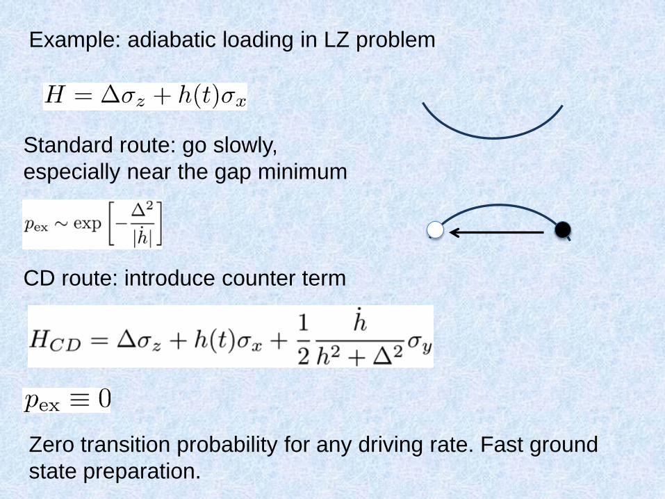
Example: adiabatic loading in LZ problem

Standard route: go slowly, especially near the gap minimum

CD route: introduce counter term

Zero transition probability for any driving rate. Fast ground state preparation.

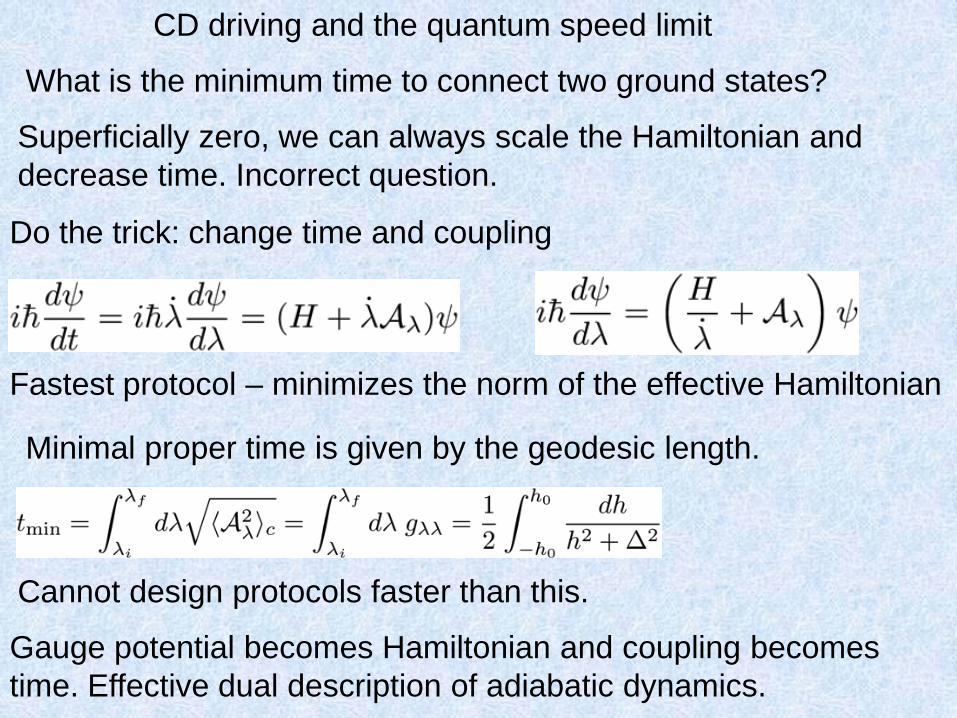
What is the minimum time to connect two ground states?

Superficially zero, we can always scale the Hamiltonian and decrease time. Incorrect question.

Do the trick: change time and coupling

Fastest protocol – minimizes the norm of the effective Hamiltonian

Minimal proper time is given by the geodesic length.

Cannot design protocols faster than this.

Gauge potential becomes Hamiltonian and coupling becomes time. Effective dual description of adiabatic dynamics.

CD driving and the quantum speed limit

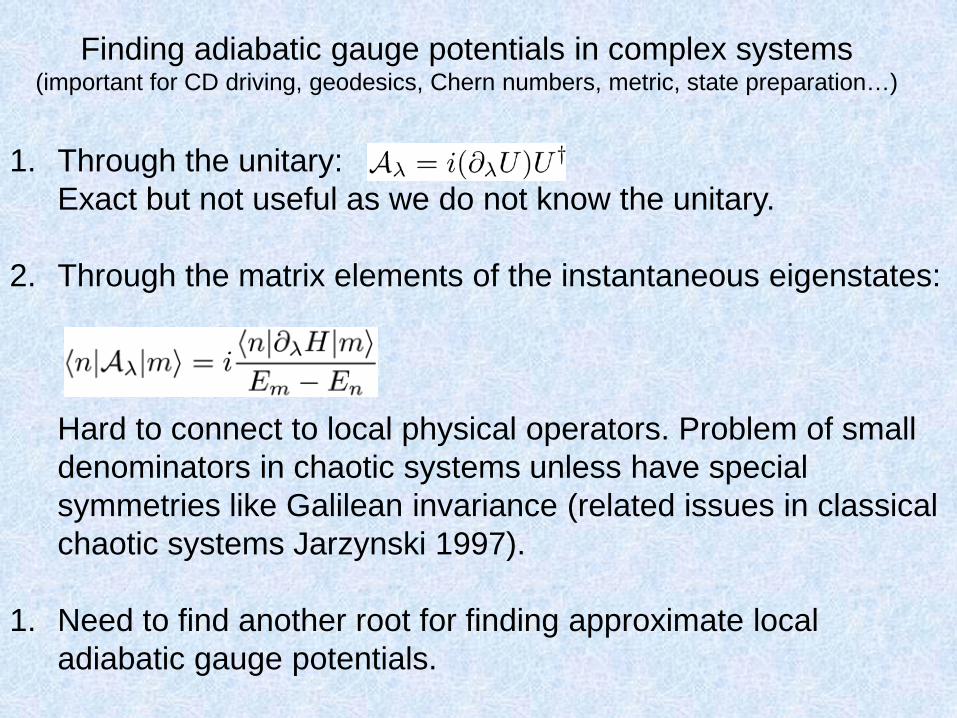
Finding adiabatic gauge potentials in complex systems (important for CD driving, geodesics, Chern numbers, metric, state preparation…)

1. Through the unitary:Exact but not useful as we do not know the unitary.

2. Through the matrix elements of the instantaneous eigenstates:

Hard to connect to local physical operators. Problem of small denominators in chaotic systems unless have special symmetries like Galilean invariance (related issues in classical chaotic systems Jarzynski 1997).

1. Need to find another root for finding approximate local adiabatic gauge potentials.

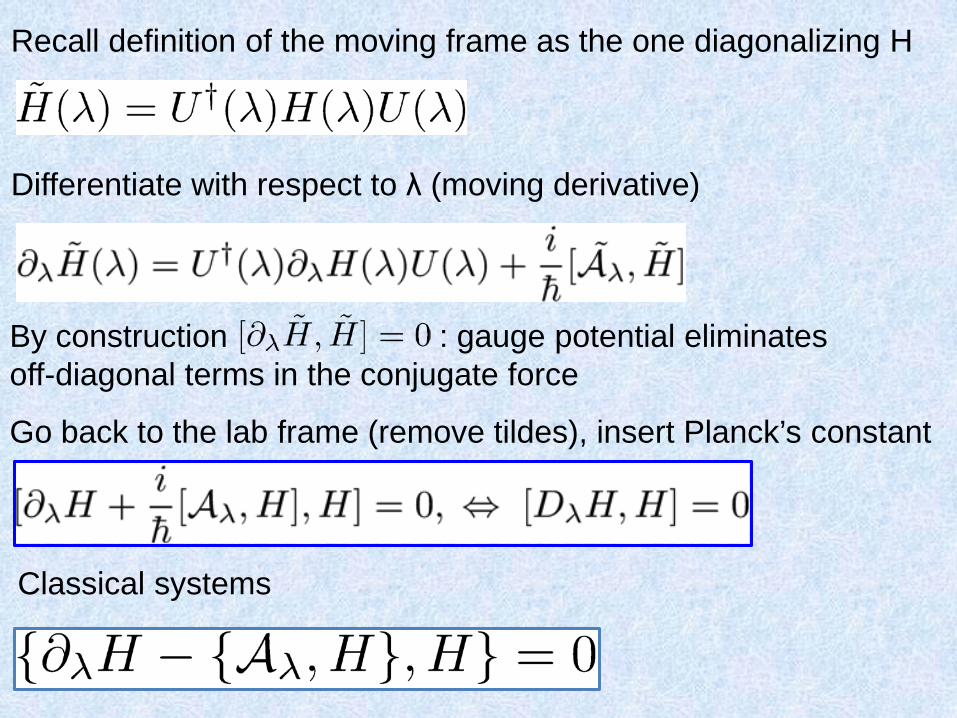
Recall definition of the moving frame as the one diagonalizing H

Differentiate with respect to λ (moving derivative)

By construction : gauge potential eliminates off-diagonal terms in the conjugate force

Go back to the lab frame (remove tildes), insert Planck’s constant

Classical systems

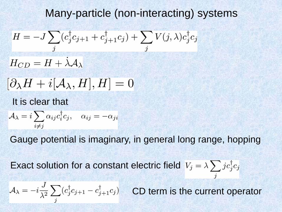
Many-particle (non-interacting) systems

It is clear that

Gauge potential is imaginary, in general long range, hopping

Exact solution for a constant electric field

CD term is the current operator

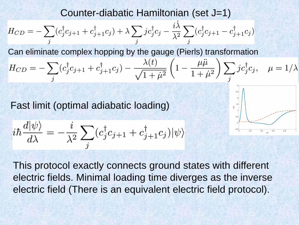
Counter-diabatic Hamiltonian (set J=1)

Can eliminate complex hopping by the gauge (Pierls) transformation

Fast limit (optimal adiabatic loading)

This protocol exactly connects ground states with different electric fields. Minimal loading time diverges as the inverse electric field (There is an equivalent electric field protocol).

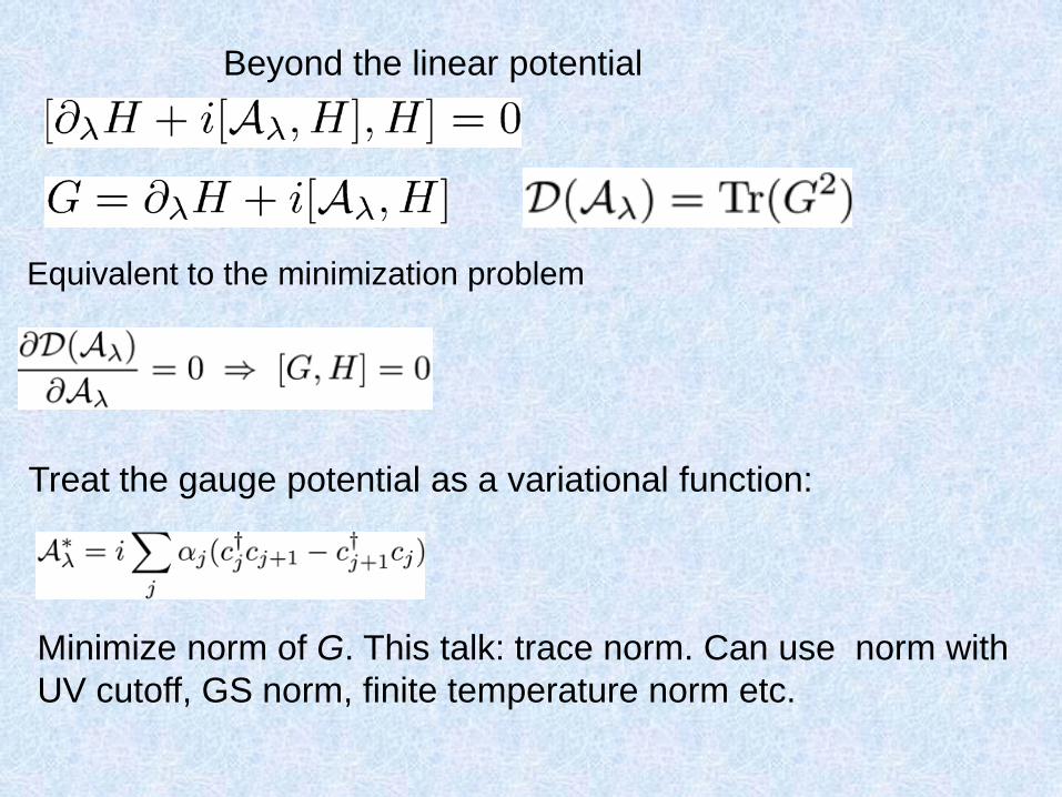
Beyond the linear potential

Treat the gauge potential as a variational function:

Minimize norm of G. This talk: trace norm. Can use norm with UV cutoff, GS norm, finite temperature norm etc.

Equivalent to the minimization problem

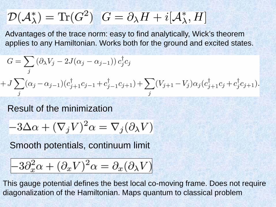
Advantages of the trace norm: easy to find analytically, Wick’s theorem applies to any Hamiltonian. Works both for the ground and excited states.

Result of the minimization

Smooth potentials, continuum limit

This gauge potential defines the best local co-moving frame. Does not require diagonalization of the Hamiltonian. Maps quantum to classical problem

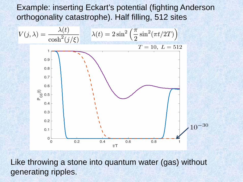
Example: inserting Eckart’s potential (fighting Anderson orthogonality catastrophe). Half filling, 512 sites

Like throwing a stone into quantum water (gas) without generating ripples.

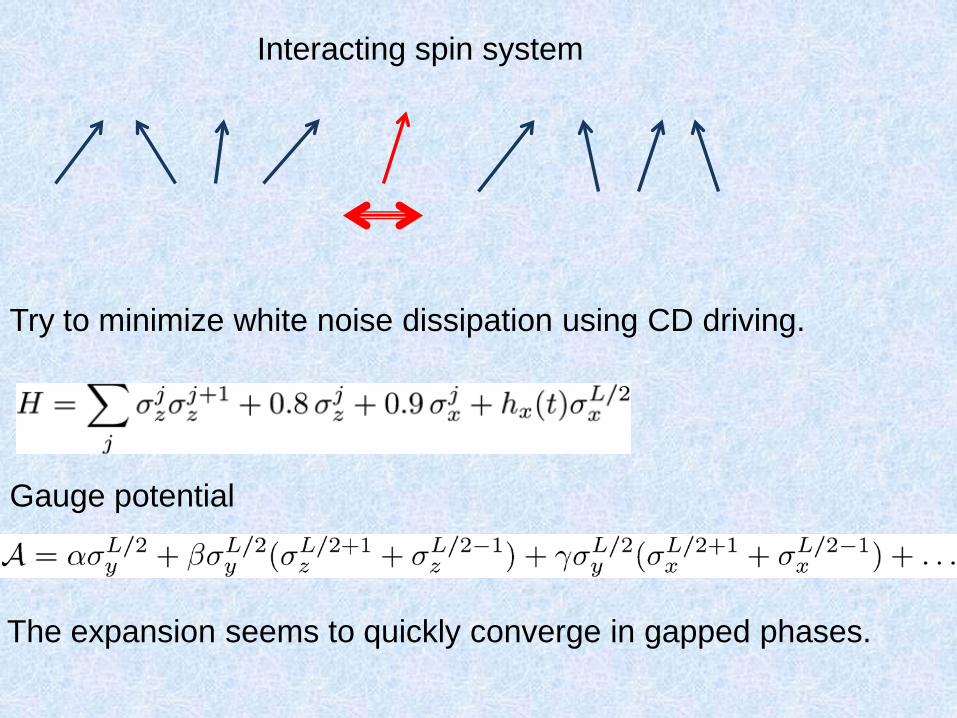
Interacting spin system

Try to minimize white noise dissipation using CD driving.

Gauge potential

The expansion seems to quickly converge in gapped phases.

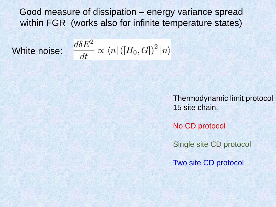
Good measure of dissipation – energy variance spread within FGR (works also for infinite temperature states)

White noise:

Thermodynamic limit protocol15 site chain.

No CD protocol

Single site CD protocol

Two site CD protocol

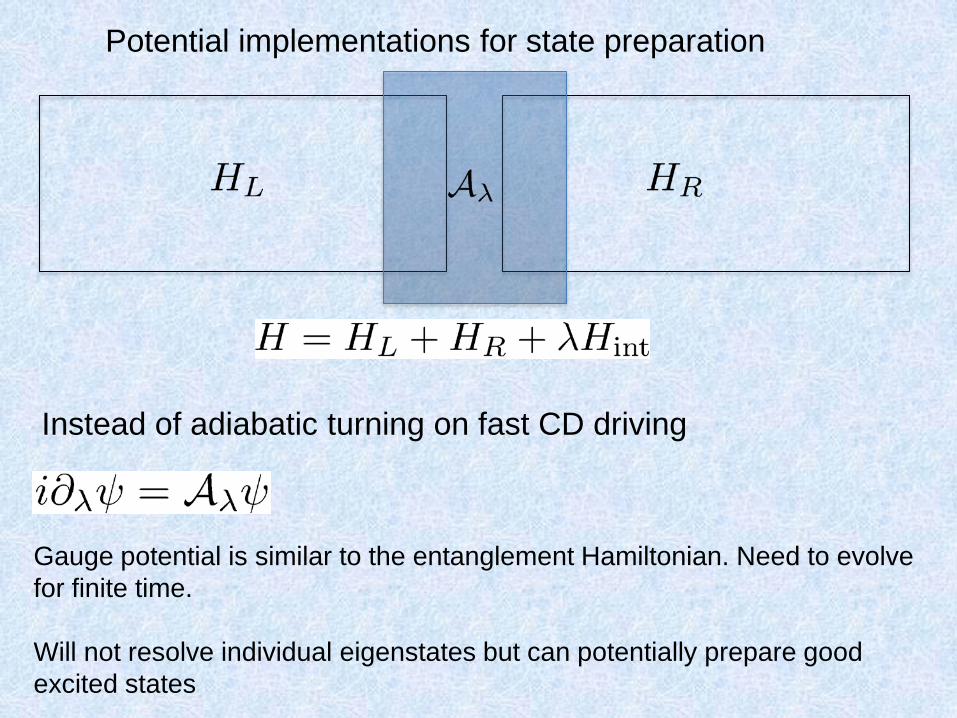
Potential implementations for state preparation

Instead of adiabatic turning on fast CD driving

Gauge potential is similar to the entanglement Hamiltonian. Need to evolve for finite time.

Will not resolve individual eigenstates but can potentially prepare good excited states

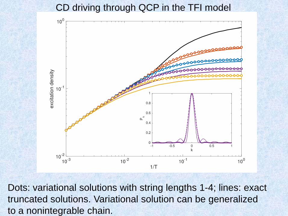
CD driving through QCP in the TFI model

Dots: variational solutions with string lengths 1-4; lines: exact truncated solutions. Variational solution can be generalized to a nonintegrable chain.

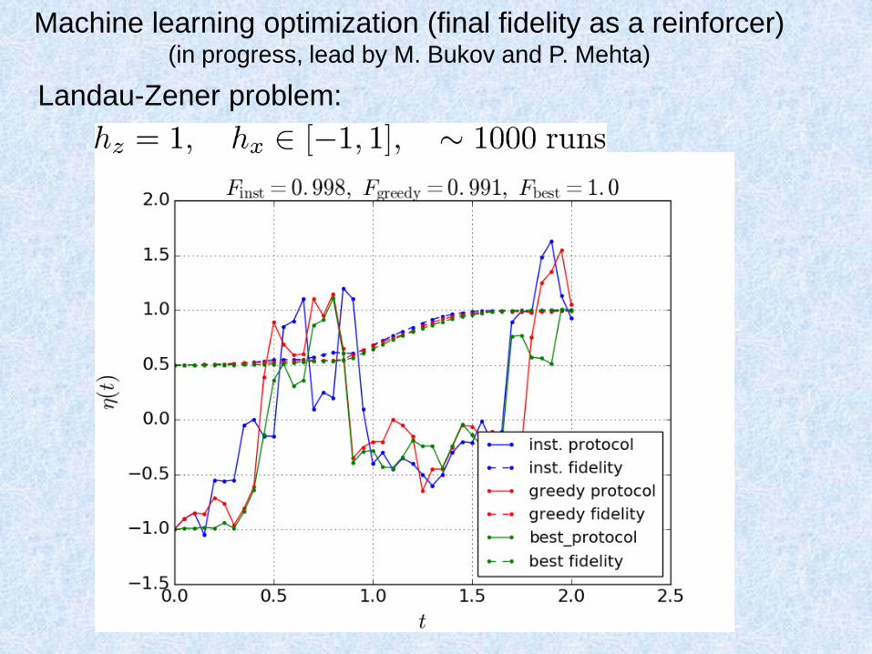
Machine learning optimization (final fidelity as a reinforcer)(in progress, lead by M. Bukov and P. Mehta)

Landau-Zener problem:

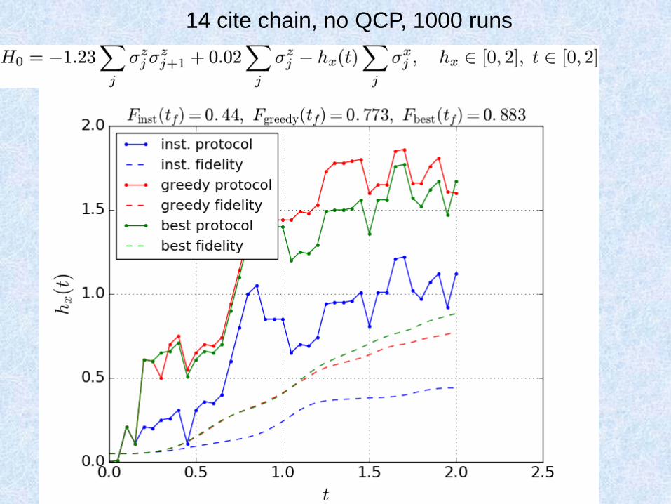
14 cite chain, no QCP, 1000 runs

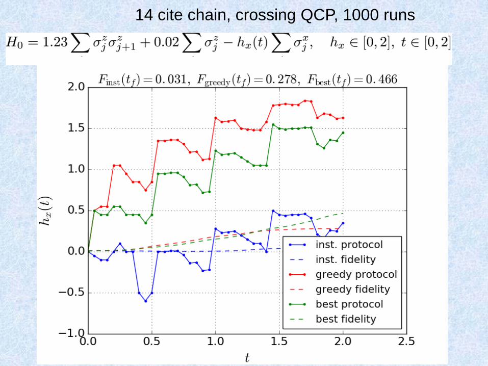
14 cite chain, crossing QCP, 1000 runs

Summary

• Deep connections between non-adiabatic response and geometry.

• Counter-adiabatic driving for quantum state preparation and suppression of dissipation.

• Many open questions/potential applications.

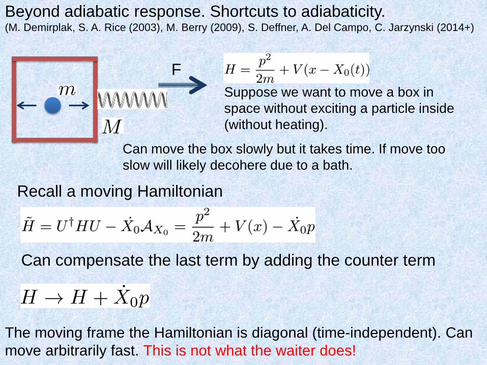
Beyond adiabatic response. Shortcuts to adiabaticity.(M. Demirplak, S. A. Rice (2003), M. Berry (2009), S. Deffner, A. Del Campo, C. Jarzynski (2014+)

FSuppose we want to move a box in space without exciting a particle inside (without heating).

Can move the box slowly but it takes time. If move too slow will likely decohere due to a bath.

Recall a moving Hamiltonian

Can compensate the last term by adding the counter term

The moving frame the Hamiltonian is diagonal (time-independent). Can move arbitrarily fast. This is not what the waiter does!

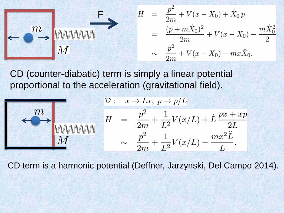
F

CD (counter-diabatic) term is simply a linear potential proportional to the acceleration (gravitational field).

CD term is a harmonic potential (Deffner, Jarzynski, Del Campo 2014).

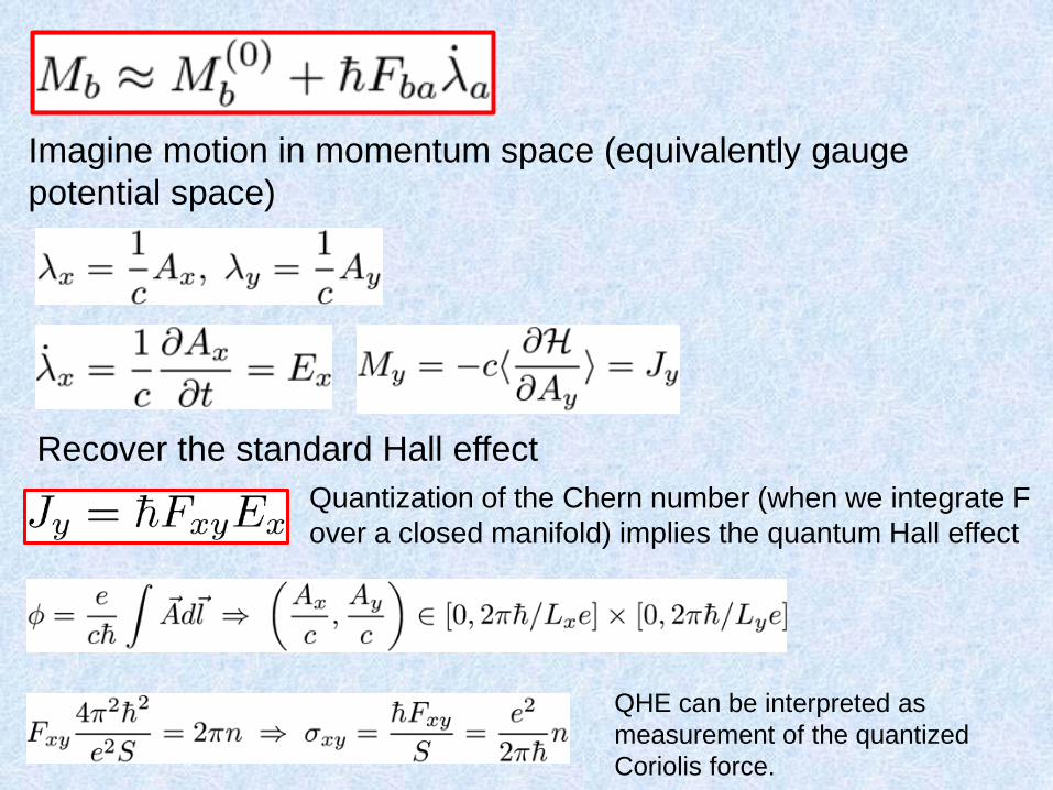
Imagine motion in momentum space (equivalently gauge potential space)

Quantization of the Chern number (when we integrate F over a closed manifold) implies the quantum Hall effect

Recover the standard Hall effect

QHE can be interpreted as measurement of the quantized Coriolis force.

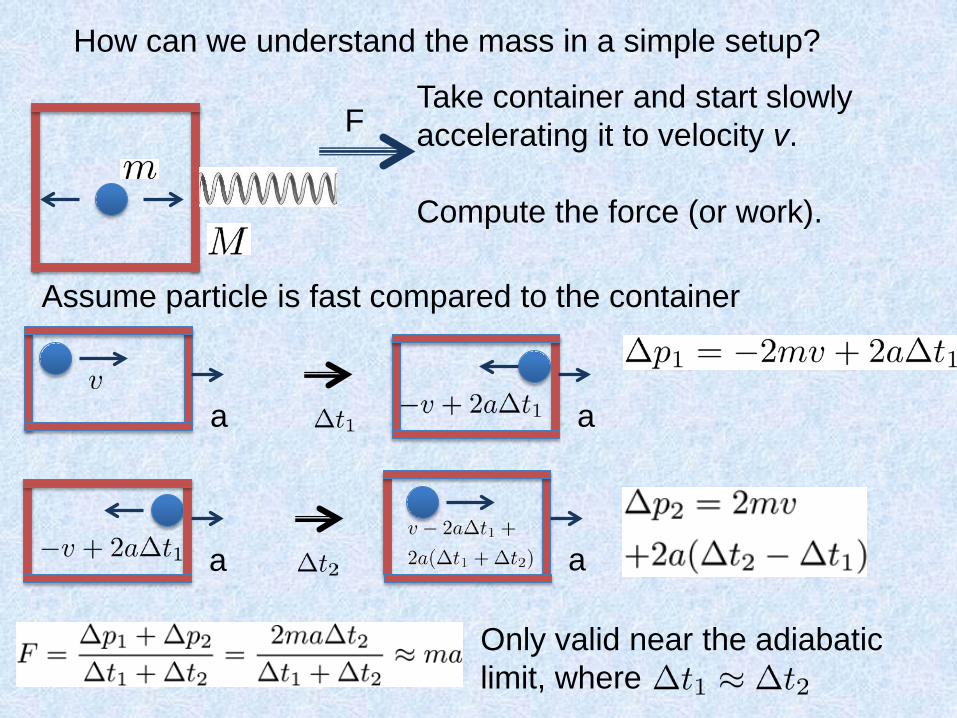
How can we understand the mass in a simple setup?

FTake container and start slowly accelerating it to velocity v.

Compute the force (or work).

Assume particle is fast compared to the container

a a

a a

Only valid near the adiabatic limit, where

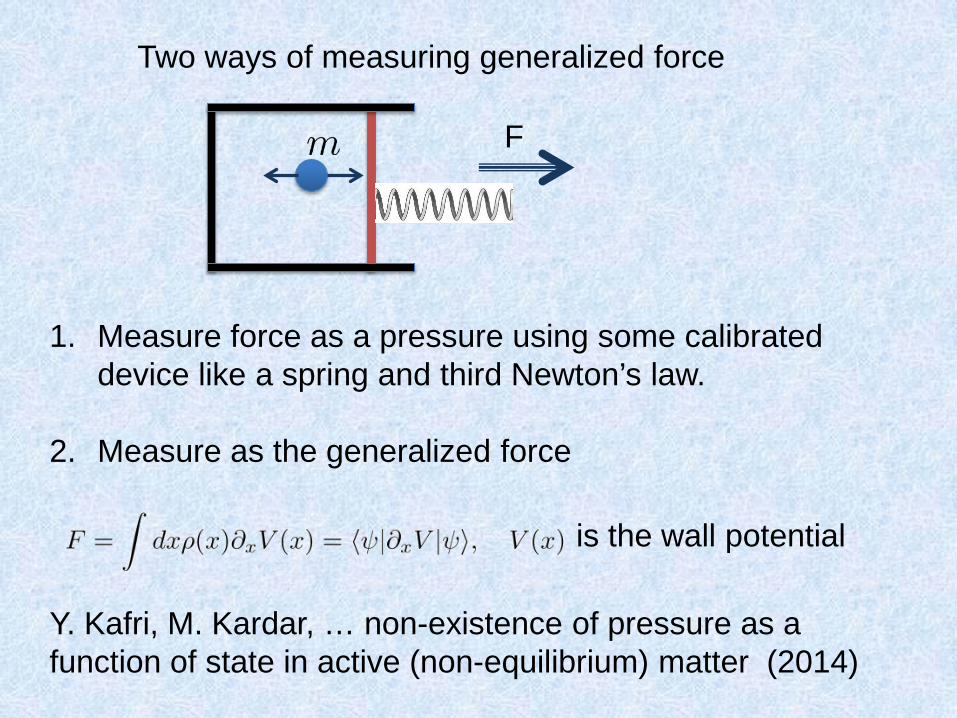
Two ways of measuring generalized force

1. Measure force as a pressure using some calibrated device like a spring and third Newton’s law.

2. Measure as the generalized force

is the wall potential

F

Y. Kafri, M. Kardar, … non-existence of pressure as a function of state in active (non-equilibrium) matter (2014)