Institut de Recerca en Economia Aplicada Regional i Pública Document de Treball 2017/16, 51 pàg.

Research Institute of Applied Economics Working Paper 2017/16, 51 pag.

Grup de Recerca Anàlisi Quantitativa Regional Document de Treball 2017/08, 51 pàg.

Regional Quantitative Analysis Research Group Working Paper 2017/08, 51 pag.

“Analyzing Wage Differentials by Fields of Study: Evidence from Turkey”

Antonio Di Paolo and Aysit Tansel

WEBSITE: www.ub-irea.com • CONTACT: irea@ub.edu

Universitat de Barcelona Av. Diagonal, 690 • 08034 Barcelona

The Research Institute of Applied Economics (IREA) in Barcelona was founded

in 2005, as a research institute in applied economics. Three consolidated

research groups make up the institute: AQR, RISK and GiM, and a large

number of members are involved in the Institute. IREA focuses on four priority

lines of investigation: (i) the quantitative study of regional and urban economic

activity and analysis of regional and local economic policies,

(ii) study of public economic activity in markets, particularly in the fields of

empirical evaluation of privatization, the regulation and competition in the

markets of public services using state of industrial economy, (iii) risk analysis in

finance and insurance, and (iv) the development of micro and macro

econometrics applied for the analysis of economic activity, particularly for

quantitative evaluation of public policies.

IREA Working Papers often represent preliminary work and are circulated to

encourage discussion. Citation of such a paper should account for its

provisional character. For that reason, IREA Working Papers may not be

reproduced or distributed without the written consent of the author. A revised

version may be available directly from the author.

Any opinions expressed here are those of the author(s) and not those of IREA.

Research published in this series may include views on policy, but the institute

itself takes no institutional policy positions.

WEBSITE: www.ub.edu/aqr/ • CONTACT: aqr@ub.edu

Abstract

This paper analyzes the drivers of wage differences among

college graduates who hold a degree in a different field of study.

We focus on Turkey, an emerging country that is characterized by

a sustained expansion of higher education. We estimate

conditional wage gaps by field of study using OLS regressions.

Average differentials are subsequently decomposed into the

contribution of observable characteristics (endowment) and

unobservable characteristics (returns). To shed light on

distributional wage disparities by field of study, we provide

estimates along the unconditional wage distribution by means of

RIF-Regressions. Finally, we also decompose the contribution of

explained and unexplained factors in accounting for wage gaps

along the whole distribution. As such, this is the first work

providing evidence on distributional wage differences by college

major for a developing country. The results indicate the existence

of important wage differences by field of study, which are partly

accounted by differences in observable characteristics (especially

occupation and, to a lesser extent, employment sector). These

pay gaps are also heterogeneous over the unconditional

distribution of wages, as is the share of wage differentials that can

be attributed to differences in observable characteristics across

workers with degrees in different fields of study.

JEL Classification: J31, J24, I23, I26. Keywords: Fields of Study, Wage Differentials, Decomposition, Unconditional

Wage Distribution, Turkey.

Aysit Tansel (corresponding author), e-mail: atansel@metu.edu.tr. Address: Department of Economics Middle East Technical University, 06800 Ankara (Turkey), telephone: +903122102073, fax: +903122107964; Institute for the Study of Labor (IZA), Bonn, Germany; Economic Research Forum (ERF) Cairo, Egypt. Antonio Di Paolo, e-mail: antonio.dipaolo@ub.edu. Address: Department of Econometrics, University of Barcelona, Avinguda Diagonal 690, 08034, Barcelona (Spain), telephone: +34934037150, fax: +34934021821. Acknowledgements Funding from the MEC grant ECO2016-75805-R is gratefully acknowledged. This paper benefited from comments received in seminars at the Atilim University (Ankara, Turkey), the Selcuk University (Konya, Turkey), the Piri Reis University (Istanbul, Turkey), as well as at the 28th EALE Conference (Ghent, Belgium), 2nd Workshop on Human Capital (Istanbul, Turkey), 37th MEEA Annual Meeting (Chicago, US) and the 4thWorkshop on the Economics, Statistics and Econometrics of Education. We also thank the suggestions received by Asena Caner. We are grateful to Murat Karakas (TURKSTAT) for his help in questions related to the data. The usual disclaimers apply.

2

1) Introduction

What drives wage disparities among university graduates who studied different

fields? There is an extensive amount of evidence documenting the general payoff to

obtaining a university degree (relative to lower education levels), but also a growing

number of papers highlighting the existing heterogeneity in the return to tertiary education

according to the field of study (see Altonji et al., 2012 and Altonji et al., 2015 for recent

overviews). However, the forces that drive wage gaps by field of study among university

graduates have not been widely explored so far and the literature focused on this specific

issue is still scarce.

Indeed, analyzing the factors that account for wage differences by field of study is

becoming an attractive area of research, since there are several policy-relevant issues that

motivate such interest. First, relative wage differences across fields of tertiary education

are likely to affect the choice of university major (see Berge, 1988, Montmarquette et al.,

2002, Bhattacharya, 2005, Beffy et al., 2012, Long et al., 2015, among others). Therefore,

providing evidence about earnings gaps across fields and, more importantly, about the

drivers of such disparities would be extremely valuable for future university students (and

their parents) when deciding about their college major. Second, insights about

determinants of earnings disparities across fields of study would be useful for academic

policies aimed at efficiently allocating economic resources across universities and

academic areas, setting tuition fees for different university programs, as well as

determining the course composition of different fields of study that will prepare students

for the labor market. This would be especially important in the context of a sustained

expansion of tertiary education, as is occurring in many developed and emerging

countries, since the supply of university graduates from different fields of study

constitutes an important input into the skill composition of the future workforce (Altonji

et al., 2015). Its efficient allocation in the economy represents a fundamental aspect for

guaranteeing a sustainable pattern of economic growth and development.

We consider the case of Turkey, a developing country that has been characterized by

a huge expansion of tertiary education over the last decades. The high and increasing

demand for university education in Turkey is mainly due to the substantially high returns

to tertiary education, compared to lower levels of schooling (see Tansel, 1994, 2001, and

2010). Indeed, during the period 2014-2016, the numbers of male (female) students

within the entire higher education system rose from 2.9 (2.1) to 3.6 (3.1) million,

3

representing substantial increases in recent years. Moreover, the Turkish case is

especially relevant, since access to university is determined by a highly selective

centralized university entrance examination. Its results determine the final placement of

applicants across different fields, degrees, and universities (for additional details, see

Caner and Okten, 2010 and Frisancho et al., 2016). Therefore, having a clear picture about

the relative monetary rewards of holding a degree in different fields of study would be

beneficial for prospective students, when carrying out the necessary investment to prepare

for the university entrance examination. Moreover, the evidence we report in this paper

could be useful for administrators, since it can serve as a basis to optimally set the

university entrance examination cut-off points associated with different disciplines. More

generally, our work represents the first contribution about the monetary value attached to

different fields of tertiary education in developing countries, since to the best of our

knowledge the existing literature is exclusively focused on developed countries.1

Our empirical analysis proceeds as follows: First, we run simple OLS regressions for

(log) real hourly wages with a set of field of study indicators. The wage equations are

estimated for male wage-earners, in order to minimize issues due to possible self-selection

into labor market participation and employment. The model is initially based on a

parsimonious specification that includes only controls for survey wave, current job

tenure, and potential experience (previous to current employment). Next, we

progressively augment the wage equation by including additional controls for family

characteristics (marital status and the number of children), job characteristics

(employment sector, a quadratic function of firm size and occupation), and regional fixed

effects (dummies for the 26 NUTS2 regions). These estimates reveal that ceteris paribus

differences in wages across fields of study are, to a certain extent, mediated by the

conditional association between wages and other observed characteristics. Third, we

investigate the factors that account for the raw wage gaps across college majors by

performing the Oaxaca-Blinder decomposition for average outcomes. This methodology

disentangles the observed average differences in hourly wages into the contribution of

observable characteristics (endowments or explained component) and the corresponding

coefficients (prices or unexplained component). A similar decomposition approach has

1 See Arcidiacono (2004), Hamermesh and Donald (2008), Altonji et al. (2012), Altonji et al. (2014), and Webber (2014) for the case of the US, Bratti et al. (2008), Chevalier (2011), and Walker and Zhu (2011) for the UK, Finnie and Frenette (2003) and Lemieux (2014) for Canada, Hasting et al. (2013) and Rodríguez et al. (2015) for Chile, Ballarino and Bratti (2009) and Buonanno and Pozzoli (2009) for Italy, Kelly et al. (2010) for Ireland, Livanos and Pouliakas (2011) for Greece, Grave and Goerlitz (2012) for Germany and Kirkebøen et al. (2016) for Norway.

4

only been applied by Grave and Goerlitz (2012) to analyze wage differences by field of

study among university graduates in Germany. However, no other paper relies on

decomposition analysis to examine the role of observed and unobserved factors in

explaining wage gaps between fields of study for university graduates2. This means that

we provide additional evidence about the drivers of average wage differences by field of

study.

The simple regressions and the corresponding decomposition provide evidence only

on the average of the wage distribution, which might hide important differentials that take

place at other points of the wage distribution than the mean. Therefore, we go a step

further by providing distributional wage gaps. There are a few papers that investigate

wage differences by field of study along the conditional wage distribution using classical

Quantile Regressions (see Hamermesh and Donald, 2008, Kelly et al., 2010, Chevalier,

2011 and Livanos and Pouliakas, 2011). In this paper, rather than considering the effect

of fields of study at different points of the conditional wage distribution, we adopt the

Unconditional Quantile Regression (UQR) approach proposed by Firpo et al. (2009). This

approach provides the wage differential of a given field relative to the chosen base

category at different points of the unconditional wage distribution. This is indeed an

important piece of evidence, since not only policy-makers but also students and parents

are more likely to be interested in the relative returns to different college majors on the

unconditional wage distribution. Such estimates can be obtained through the Recentered

Influence Function (RIF) Regression. It yields estimates of Unconditional Quantile

Partial Effects of holding a degree in a given field. This novel approach has never been

applied in the literature on fields of study, and thus represents an important contribution

of this paper. Therefore, in a subsequent step, we decompose the gaps observed at

different points of the unconditional wage distribution using the decomposition method

based on RIF-Regressions (Firpo et al., 2007). The decomposition based on RIF-

Regressions extends the classical Oaxaca-Blinder decomposition3 by disentangling the

explained and unexplained components of the wage gap by field of study at different

points of the unconditional wage distribution. The evidence from this distributional

decomposition is informative, since the relative role of returns and endowments in

explaining wage differences across fields of study is likely to depend on the point of the

2 It seems also worth mentioning that Lemieux (2014) decomposed the wage gap between high school graduates and university graduates in a given field, focusing on the role of occupation and its relationship to the field of study. 3 Moreover, the RIF-based decomposition is not path-dependent and allows for a detailed analysis of the contribution of separate covariates (and the corresponding coefficients) on the distributional wage gap.

5

wage distribution at which they are evaluated. As such, our RIF-based decomposition

analysis of wage gaps by field of study constitutes the last remarkable value-added of our

work with respect to the existing research.

Although informative about the role of explained and unexplained factors in

accounting for the wage gaps across different disciplines, it seems worth recognizing that

our approach remains subject to one of the main challenges in the estimation of the wage

effect of holding a degree in a given subject: the issue of self-selection into different

disciplines based on unobservable characteristics. There are very few papers that

explicitly deal with this issue. The endogeneity of the choice of field of study has been

approached by means of structural economic models by Arcidiacono (2004) and more

recently, by Kinsler and Pavan (2015). An alternative and promising approach is based

on exploiting discontinuities induced by test-score based university admission,4 which

generates a random variation in the choice of university-subject combinations. Variants

of this general strategy have been developed by Hastings et al. (2013) for Chile and by

Kirkebøen et al. (2016) for Norway. In both countries, university entrance is ruled by a

centralized admission process and, more importantly, it is possible to link administrative

information about exam performance, college choice, and preferences with future

earnings. This enables estimating the causal effect of completing the degree in a given

subject, net of the effect of selection into fields and into next-best alternatives (Kirkebøen

et al., 2016). Although university entrance in Turkey is managed in a similar way,

combining college application data with information on post-graduate labor market

outcomes is unfortunately still unfeasible for this country. Consequently, we are forced

to rely on conditional correlations (as is done in the majority of related works) and to

interpret the unexplained component of wage differentials across fields as the composite

impact of returns to observable characteristics and selection-on-unobservable

characteristics. In our view, although clearly representing a second-best solution, the

results from our approach are still informative about the drivers of wage differences by

the field of study, and will highlight the factors that should be better investigated in causal

terms when more detailed data become available.

The rest of the paper proceeds as follows: in Section 2 we describe the data and

present some descriptive statistics, in Section 3 we explain the empirical methodology

4 Additionally, Ketel et al. (2016) analyzed the return to being admitted to a medical school in the Netherlands, which is based on a lottery mechanism that enables relying on randomization to remove self-selection in the choice of the field of study.

6

that is applied in the empirical analysis, in Section 4 we present and discuss the results

for average wage differentials (4.1) and distributional wage differentials (4.2) and finally

we conclude in Section 5.

2) Data Description

The empirical analysis is based on annual repeated cross-sections of data from the

Turkish Household Labor Force Survey (HLFS), covering the period 2009-2015.

Although the HLFS database is also available for previous years, 2009 is the first wave

in which a question about the individual’s field of study is included. The survey originally

considers 20 different categories for fields of study (plus one category for military/police

career studies5). We regrouped them into 15 categories due to small sample sizes in some

fields in the original classification. We select only tertiary educated males who are

regularly employed as wage-earners at the time of the survey.6 We retain only individuals

employed full-time who work no less than 30 hours and no more than 72 hours per week.

Individuals who are either older than 65 or younger than 23 are excluded from the final

sample, as well as those who are enrolled in education at the time of the survey.

Observations with real monthly wages (in 2010 prices) lower than 600 Turkish Liras (TL)

are discarded, which implies eliminating individuals who earn a salary lower than the

minimum wage set in 2010. Migrants and Turkish returning emigrants who returned after

completing tertiary education are also excluded from the analysis. After cleaning for

missing values in relevant variables, we end up with a pooled sample of 77,154

observations.

Our dependent variable is the log of hourly real wages from the main job in terms of

2010 prices. The database contains information on monthly wages, which are net of taxes

and include extra compensations such as bonuses and premiums in addition to salary. In

order to construct hourly wages, we exploit the information on “typical” hours of work

per week, which are converted into monthly hours of work by applying a factor of 4.3.

Table A1 in the Appendix displays the distribution of college major across survey waves,

5 We excluded individuals who graduated in this field, since they are mostly in the army or police forces and their labor market outcomes are hardly comparable with the results of their counterparts in other fields of study. 6 This restriction implies that we aim at obtaining evidence for the (male) working population, which should not be taken as representative for the whole population of individuals in the labor force because of potential self-selection into employment. For this reason, we rely only on the male subsample, since this selectivity issue should be less pronounced for males than for females even among tertiary educated individuals.

7

as well as for the pooled sample (2009-2015).7 The raw data indicate that business and

management is the most common field of study (27%), followed by education and

engineering each accounting for about 15% of the pooled sample. Further, the fields of

education, arts, humanities, personal services, architecture, agriculture & veterinary, and

health have all lost importance over the period 2009-2015, while the share of observations

in business & management, engineering, and (to a lesser extent) manufacturing increased

over time during the same period.

Kernel density estimates of the (log) hourly real wage by fields of study are reported

in Figure 1. In order to facilitate the visualization of distributional wage differences across

different fields of study, we present two graphs. Figure 1a presents the results for the

broad areas of humanities and social sciences. Figure 1b presents the results for hard

sciences, technical disciplines, and health-related fields. The former figure shows that the

wage distribution in the fields of education and humanities are very concentrated around

the mean (log) hourly wage of about 2.3 (which corresponds to an average real hourly

wage of about 10 TL). Graduates in arts and, to a lesser extent, in personal services and

business & management are the least paid, since they are mostly represented in the lowest

tail of the hourly wage distribution. Graduates in (other) social sciences and services fall

in an intermediate position, whereas graduates in law display a wage distribution that is

significantly shifted towards the right tail indicating that law is a highly rewarded field

(at least without conditioning for individual characteristics). Figure 1b indicates that

graduates in computing, manufacturing, and engineering are more represented in the

lower part of the unconditional hourly wage distribution. In contrast, those who studied

for a degree in hard sciences, mathematics & statistics, architecture, and agriculture &

veterinary are placed in an intermediate position and their wages are mostly concentrated

around the mean. Similar to the case of law, the hourly wage distribution of graduates in

health disciplines is significantly shifted towards the right, with an important proportion

of observations concentrated at the top of the overall unconditional hourly wage

distribution. The analysis of the unconditional wage distribution by field of study reveals

that different degrees are unevenly rewarded in the labor market. Moreover, wage

differences across fields operate not only on the average, but also along the wage

distribution. In the next section we investigate the drivers of such average and

7 Descriptive statistics for the variables used in the empirical analysis are reported in Table A2 in the Appendix. Notice that the information about occupation and sector has been recorded into more aggregated categories, in order to avoid small or empty cells for certain occupations/sectors (especially in those fields where the distribution of these variables is highly concentrated into specific categories).

8

distributional wage differentials by fields of study using regression and decomposition

tools.

3) Empirical Methodology

3.1) Average Wage Differentials

The starting point of our analysis of wage differentials by fields of study consists of a

simple OLS regression that explains (logged) real hourly wages (ln(wi)) as a function of

a vector of control variables (Xi) and a set of dummies for each field of study (FSi):

ln(𝑤𝑤𝑖𝑖) = 𝛼𝛼 + 𝛽𝛽′𝑋𝑋𝑖𝑖 + ∑ 𝛿𝛿𝑗𝑗𝐼𝐼(𝐹𝐹𝐹𝐹𝑖𝑖 = 𝑗𝑗) + 𝜀𝜀𝑖𝑖𝑗𝑗 𝑗𝑗 = 1 … 𝐽𝐽 − 1. (1)

Here δj represent the coefficients of interest, which measure the percentage wage

difference of holding a degree in field “j” relative to the reference category (in our case,

the field of “business and management”). We first present the estimates of δj without

conditioning for any observable characteristics, which yield unconditional wage

differences across different fields of study. Second, we progressively expand the vector

of covariates, moving from a regression that contains only the basic set of controls

(current job tenure and previous potential experience, both in quadratic form, plus survey

wave dummies), which is subsequently augmented by family characteristics, sector

dummies and firm size (in quadratic form), occupation dummies and NUTS2 region

dummies. This stepwise inclusion of control variables yields different estimates of the

“ceteris paribus” wage differentials by college major, and allows to assess whether the

raw wage differences observed across different fields of study are, to some extent,

mediated by other observable characteristics of the individual, his job, and his region of

residence, which might co-vary with both fields of study and salaries.

In order to better appreciate the contribution of observable characteristics on the

observed wage disparities between individuals who graduated from different fields, we

apply the Oaxaca-Blinder (OB) decomposition for average wage gaps (Oaxaca, 1973,

Blinder, 1973). This well-known decomposition method disentangles average outcome

differentials into the contribution of the (average) endowment of observable

characteristics (i.e. the explained or composition component) and the contribution of

9

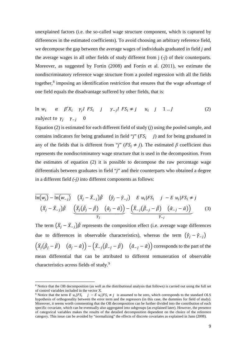
unexplained factors (i.e. the so-called wage structure component, which is captured by

differences in the estimated coefficients). To avoid choosing an arbitrary reference field,

we decompose the gap between the average wages of individuals graduated in field j and

the average wages in all other fields of study different from j (-j) of their counterparts.

Moreover, as suggested by Fortin (2008) and Fortin et al. (2011), we estimate the

nondiscriminatory reference wage structure from a pooled regression with all the fields

together,8 imposing an identification restriction that ensures that the wage advantage of

one field equals the disadvantage suffered by other fields, that is:

ln(𝑤𝑤𝑖𝑖) = 𝛼𝛼 + 𝛽𝛽′𝑋𝑋𝑖𝑖 + 𝛾𝛾𝑗𝑗𝐼𝐼(𝐹𝐹𝐹𝐹𝑖𝑖 = 𝑗𝑗) + 𝛾𝛾−𝑗𝑗𝐼𝐼(𝐹𝐹𝐹𝐹𝑖𝑖 ≠ 𝑗𝑗) + 𝑢𝑢𝑖𝑖 𝑗𝑗 = 1 … 𝐽𝐽 (2)

𝑠𝑠𝑢𝑢𝑠𝑠𝑗𝑗𝑠𝑠𝑠𝑠𝑠𝑠 𝑠𝑠𝑡𝑡 𝛾𝛾𝑗𝑗 + 𝛾𝛾−𝑗𝑗 = 0

Equation (2) is estimated for each different field of study (j) using the pooled sample, and

contains indicators for being graduated in field “j” (𝐹𝐹𝐹𝐹𝑖𝑖 = 𝑗𝑗) and for being graduated in

any of the fields that is different from “j” (𝐹𝐹𝐹𝐹𝑖𝑖 ≠ 𝑗𝑗). The estimated β coefficient thus

represents the nondiscriminatory wage structure that is used in the decomposition. From

the estimates of equation (2) it is possible to decompose the raw percentage wage

differentials between graduates in field “j” and their counterparts who obtained a degree

in a different field (-j) into different components as follows:

ln�𝑤𝑤𝚥𝚥��������� − ln�𝑤𝑤−𝚥𝚥����������� = �𝑋𝑋�𝑗𝑗 − 𝑋𝑋�−𝑗𝑗��̂�𝛽 + �𝛾𝛾�𝑗𝑗 − 𝛾𝛾�−𝑗𝑗� + 𝐸𝐸[𝑢𝑢𝑖𝑖|𝐹𝐹𝐹𝐹𝑖𝑖 = 𝑗𝑗] − 𝐸𝐸[𝑢𝑢𝑖𝑖|𝐹𝐹𝐹𝐹𝑖𝑖 ≠ 𝑗𝑗]

= �𝑋𝑋�𝑗𝑗 − 𝑋𝑋�−𝑗𝑗��̂�𝛽 + [�𝑋𝑋�𝑗𝑗��̂�𝛽𝑗𝑗 − �̂�𝛽� + �𝛼𝛼�𝑗𝑗 − 𝛼𝛼��������������������𝛾𝛾�𝑗𝑗

− �𝑋𝑋�−𝑗𝑗��̂�𝛽−𝑗𝑗 − �̂�𝛽� + �𝛼𝛼�−𝑗𝑗 − 𝛼𝛼���]�������������������𝛾𝛾�−𝑗𝑗

(3)

The term �𝑋𝑋�𝑗𝑗 − 𝑋𝑋�−𝑗𝑗��̂�𝛽 represents the composition effect (i.e. average wage differences

due to differences in observable characteristics), whereas the term �𝛾𝛾�𝑗𝑗 − 𝛾𝛾�−𝑗𝑗� =

�𝑋𝑋�𝑗𝑗��̂�𝛽𝑗𝑗 − �̂�𝛽� + �𝛼𝛼�𝑗𝑗 − 𝛼𝛼��� − �𝑋𝑋�−𝑗𝑗��̂�𝛽−𝑗𝑗 − �̂�𝛽� + �𝛼𝛼�−𝑗𝑗 − 𝛼𝛼��� corresponds to the part of the

mean differential that can be attributed to different remuneration of observable

characteristics across fields of study.9

8 Notice that the OB decomposition (as well as the distributional analysis that follows) is carried out using the full set of control variables included in the vector X. 9 Notice that the term 𝐸𝐸[𝑢𝑢𝑖𝑖|𝐹𝐹𝐹𝐹𝑖𝑖 = 𝑗𝑗] − 𝐸𝐸[𝑢𝑢𝑖𝑖|𝐹𝐹𝐹𝐹𝑖𝑖 ≠ 𝑗𝑗] is assumed to be zero, which corresponds to the standard OLS hypothesis of orthogonality between the error term and the regressors (in this case, the dummies for field of study). Moreover, it seems worth commenting that the OB decomposition can be further divided into the contribution of each specific covariate, which can be eventually also aggregated into subgroups (as explained later). However, the presence of categorical variables makes the results of the detailed decomposition dependent on the choice of the reference category. This issue can be avoided by “normalizing” the effects of discrete covariates as explained in Jann (2008).

10

3.2) Distributional Wage Differentials

It seems worth noting that both the regression analysis and the OB decomposition

provide evidence about average wage differences across college majors. However, as

commented in the introduction (and confirmed by the graphical analysis of the wage

distribution by field of study), focusing on average gaps could hide important disparities

that could occur in other parts of the wage distribution than the mean. To evaluate

distributional wage disparities across fields of study, we estimate the Unconditional

Quantile Regression (UQR) proposed by Firpo et al. (2009). The UQR method is based

on the statistical concept of Influence Function (IF), which represents the influence of an

individual observation on a distributional statistic of interest (e.g. the quantile). By adding

back the statistic to the corresponding IF, it is possible to obtain the Recentered Influence

Function (RIF) for each quantile of the outcome. Specifically, the RIF for the τth quantile

(𝑞𝑞𝜏𝜏) of logged hourly wages corresponds to,

𝑅𝑅𝐼𝐼𝐹𝐹(ln(𝑤𝑤𝑖𝑖) , 𝑞𝑞𝜏𝜏) = 𝑞𝑞𝜏𝜏 + 𝐼𝐼𝐹𝐹(ln(𝑤𝑤𝑖𝑖) , 𝑞𝑞𝜏𝜏) = 𝑞𝑞𝜏𝜏 + 𝜏𝜏−𝐼𝐼(ln(𝑤𝑤𝑖𝑖)≤ 𝑞𝑞𝜏𝜏)𝑓𝑓ln(𝑤𝑤)(𝑞𝑞𝜏𝜏)

(4)

where I(·) is an indicator function and 𝑓𝑓ln(𝑤𝑤)(𝑞𝑞𝜏𝜏) is the density of the marginal

(unconditional) distribution of the outcome (ln(𝑤𝑤)) evaluated at 𝑞𝑞𝜏𝜏. The estimated

counterpart of the RIF is simply obtained by replacing the unknown components by their

sample estimators, such as,

𝑅𝑅𝐼𝐼𝐹𝐹� (ln(𝑤𝑤𝑖𝑖) , 𝑞𝑞�𝜏𝜏) = 𝑞𝑞�𝜏𝜏 + 𝐼𝐼𝐹𝐹�(ln(𝑤𝑤𝑖𝑖) , 𝑞𝑞�𝜏𝜏) = 𝑞𝑞�𝜏𝜏 + 𝜏𝜏−𝐼𝐼(ln(𝑤𝑤𝑖𝑖)≤ 𝑞𝑞�𝜏𝜏)�̂�𝑓ln(𝑤𝑤)(𝑞𝑞�𝜏𝜏)

(5)

Where 𝑓𝑓ln(𝑤𝑤)(𝑞𝑞�𝜏𝜏) corresponds to a kernel density estimator of the unconditional density

function of the outcome. The RIF for a given quantile can be taken as a linear

approximation of the nonlinear function of the quantile, and captures the change of the

(unconditional) quantile of the outcome in response to a change in the underlying

distribution of the covariates (Firpo et al., 2009). In fact, it can be shown that the expected

value of the RIF can be modelled to be a linear function of explanatory variables, as in a

standard linear regression. Therefore, it is possible to analyze wage disparities by field of

11

study along the (unconditional) wage distribution by specifying the following linear UQR

for selected quantiles of the unconditional distribution of real hourly wages (𝑞𝑞�𝜏𝜏):

𝐸𝐸[𝑅𝑅𝐼𝐼𝐹𝐹� (ln(𝑤𝑤𝑖𝑖) , 𝑞𝑞�𝜏𝜏)|𝑋𝑋𝑖𝑖,𝐹𝐹𝐹𝐹𝑖𝑖] = 𝛼𝛼�𝜏𝜏 + �̂�𝛽𝜏𝜏′𝑋𝑋𝑖𝑖 + ∑ 𝛿𝛿𝑗𝑗𝜏𝜏𝐼𝐼(𝐹𝐹𝐹𝐹𝑖𝑖 = 𝑗𝑗)𝑗𝑗 𝑗𝑗 = 1 … 𝐽𝐽 − 1. (6)

The estimates of 𝛿𝛿𝑗𝑗𝜏𝜏 from equation (6) represents the marginal impact of a small change

in the probability of holding a degree in field “j” (relative to the reference field) on the

unconditional τ-quantile of logged hourly wages.

Given the linear approximation of the conditional expectation of the RIF and the

theoretical property stating that the average 𝑅𝑅𝐼𝐼𝐹𝐹������ln�𝑤𝑤𝑗𝑗� , 𝑞𝑞�𝜏𝜏� is equal to the

corresponding marginal quantile of the distribution of the outcome (𝑞𝑞�𝑗𝑗𝜏𝜏), it is possible to

generalize the standard OB decomposition of average outcomes to a distributional

decomposition applied to the unconditional distribution of the outcome (see Firpo et al.,

2007 and Fortin et al., 2011 for technical details). Put in other words, it is possible to

examine the contribution of the endowment of observable characteristics and the returns

to these characteristics in explaining the estimated unconditional wage gap across fields

of study, applying the outcome decomposition for average outcomes described by

equation (3) to the RIF, that is:

𝑞𝑞�𝑗𝑗𝜏𝜏 − 𝑞𝑞�−𝑗𝑗𝜏𝜏 = 𝑅𝑅𝐼𝐼𝐹𝐹������ln�𝑤𝑤𝑗𝑗� , 𝑞𝑞�𝜏𝜏� − 𝑅𝑅𝐼𝐼𝐹𝐹������ln�𝑤𝑤−𝑗𝑗� , 𝑞𝑞�𝜏𝜏� =

�𝑋𝑋�𝑗𝑗 − 𝑋𝑋�−𝑗𝑗��̂�𝛽𝜏𝜏 + ��𝑋𝑋�𝑗𝑗��̂�𝛽𝑗𝑗𝜏𝜏 − �̂�𝛽𝜏𝜏� + �𝛼𝛼�𝑗𝑗𝜏𝜏 − 𝛼𝛼�𝜏𝜏�� − �𝑋𝑋�−𝑗𝑗��̂�𝛽−𝑗𝑗𝜏𝜏 − �̂�𝛽𝜏𝜏� + �𝛼𝛼�−𝑗𝑗𝜏𝜏 − 𝛼𝛼�𝜏𝜏��� (7)

Here �̂�𝛽𝜏𝜏 corresponds to the nondiscriminatory wage structure (estimated from a pooled

RIF regression) at quantile τ estimated in a similar fashion as equation (2) using the

estimated RIF for individuals graduated in field “j” and in fields different than “j” as

dependent variable. Similar to equation (3), the term �𝑋𝑋�𝑗𝑗 − 𝑋𝑋�−𝑗𝑗��̂�𝛽𝜏𝜏 represents the

composition effect and the term �𝑋𝑋�𝑗𝑗��̂�𝛽𝑗𝑗𝜏𝜏 − �̂�𝛽𝜏𝜏� + �𝛼𝛼�𝑗𝑗𝜏𝜏 − 𝛼𝛼�𝜏𝜏�� − �𝑋𝑋�−𝑗𝑗��̂�𝛽−𝑗𝑗𝜏𝜏 − �̂�𝛽𝜏𝜏� +

�𝛼𝛼�−𝑗𝑗𝜏𝜏 − 𝛼𝛼�𝜏𝜏�� captures the unexplained component of the percentage wage differential

evaluated at the τ-quantile of the unconditional distribution of (logged) wages.

12

4) Estimation Results

4.1) Average Wage Differentials

The main results from the OLS estimation of equation (1) are reported in Table 2

(complete results are displayed in Table A3 in the Appendix). The estimates in column

(1) are obtained without conditioning on observable characteristics and express

percentage differences in real hourly wages relative to graduates in business &

management,10 which is the reference and the most common field of study. Graduates in

manufacturing (-14.1%), computing (-12.1%) and, to a lesser extent, in personal services

(-8.8%), arts (-7.9%), and engineering (-5.2%) obtain a lower average remuneration than

graduates in business and management. All the other fields are better paid than the

reference group. The unconditional wage differential is especially pronounced for health

(+64.6%) and law (+55%), which are followed by hard sciences (+13.7%), social sciences

and education (+12.9%), mathematics & statistics (+12%), agriculture & veterinary

(+11%), humanities (+8.5%), and architecture (+7.3%). Thus, manufacturing is the

lowest and health is the highest paid field of study compared to business & management.

In Column (2) we control for the survey wave, current job tenure, and previous

potential experience, where the latter two variables enter in a quadratic form. In this way

we account for the fact that graduates in different fields of study may have different career

profiles in terms of tenure and work experience, as well as for the changing distribution

of university graduates across fields of study over time. Indeed, some of the negative

differentials relative to graduates in business & management either change sign (i.e.

computing), disappear (i.e. engineering), or are mitigated (as for manufacturing and arts).

The positive differential observed in favor of graduates in education, law, social sciences,

agriculture & veterinary, and health is lower when controlling for the basic set of

covariates, and reverts sign for the field of humanities.

Accounting for family characteristics, namely marital status and the number of

children, has virtually no effect on the coefficients associated with different fields of study

(see in Column (3)). This suggests that family structure and cohabitation do not drive

wage disparities between individuals graduated in different disciplines. The results

indicate that graduates in education, law, social sciences & services, mathematics &

10 The average of (log) real hourly wages for graduates in business & management is equal to 2.15 (i.e. hourly wage in 2010 prices equal to 9.97 TL), which is around 8.1% lower than the overall average.

13

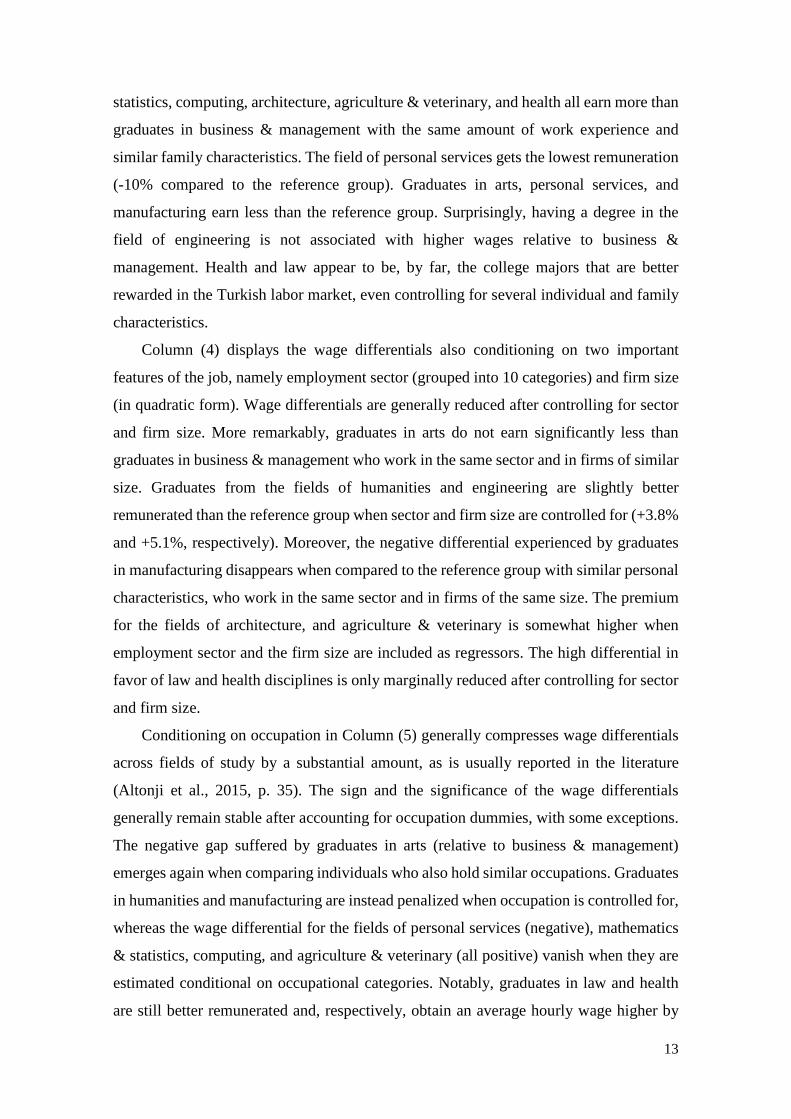
statistics, computing, architecture, agriculture & veterinary, and health all earn more than

graduates in business & management with the same amount of work experience and

similar family characteristics. The field of personal services gets the lowest remuneration

(-10% compared to the reference group). Graduates in arts, personal services, and

manufacturing earn less than the reference group. Surprisingly, having a degree in the

field of engineering is not associated with higher wages relative to business &

management. Health and law appear to be, by far, the college majors that are better

rewarded in the Turkish labor market, even controlling for several individual and family

characteristics.

Column (4) displays the wage differentials also conditioning on two important

features of the job, namely employment sector (grouped into 10 categories) and firm size

(in quadratic form). Wage differentials are generally reduced after controlling for sector

and firm size. More remarkably, graduates in arts do not earn significantly less than

graduates in business & management who work in the same sector and in firms of similar

size. Graduates from the fields of humanities and engineering are slightly better

remunerated than the reference group when sector and firm size are controlled for (+3.8%

and +5.1%, respectively). Moreover, the negative differential experienced by graduates

in manufacturing disappears when compared to the reference group with similar personal

characteristics, who work in the same sector and in firms of the same size. The premium

for the fields of architecture, and agriculture & veterinary is somewhat higher when

employment sector and the firm size are included as regressors. The high differential in

favor of law and health disciplines is only marginally reduced after controlling for sector

and firm size.

Conditioning on occupation in Column (5) generally compresses wage differentials

across fields of study by a substantial amount, as is usually reported in the literature

(Altonji et al., 2015, p. 35). The sign and the significance of the wage differentials

generally remain stable after accounting for occupation dummies, with some exceptions.

The negative gap suffered by graduates in arts (relative to business & management)

emerges again when comparing individuals who also hold similar occupations. Graduates

in humanities and manufacturing are instead penalized when occupation is controlled for,

whereas the wage differential for the fields of personal services (negative), mathematics

& statistics, computing, and agriculture & veterinary (all positive) vanish when they are

estimated conditional on occupational categories. Notably, graduates in law and health

are still better remunerated and, respectively, obtain an average hourly wage higher by

14

31% and 40.5% than the reference category even controlling for occupation. The

estimates are mostly unaffected by the further inclusion of fixed effects for 26 NUTS2

regions of Turkey as shown in Column (6). This suggests that local differences in the

labor market do not significantly affect wage disparities between tertiary educated

workers with different college majors. The exceptions are manufacturing, for which the

negative differential disappears after conditioning on regions, and agriculture &

veterinary, which is slightly more rewarded than business & management.

We also repeated the OLS estimation for the full specification of the wage equation

splitting the sample into three age groups namely 23-30, 31-40, and 41-65. These results

are reported in Table A3 in the Appendix. This exercise provides a picture of the relative

pay differentials across disciplines at different stages of the career. There are remarkable

differences over the life-cycle for humanistic disciplines. Namely, the premium

associated with education is mostly captured by young workers, who earn 13.2% more

than their counterparts of the same age cohort who graduated in business & management,

while the oldest group of workers in this field suffers an earnings penalty. A similar

pattern is observed for arts, since young graduates in this field are better paid than the

reference field, while the opposite is true for the older cohorts. The premium for graduates

in social sciences and architecture vanishes in advanced stages of the working career. On

the contrary, the premium for the fields of law, computing, manufacturing, health, and to

a lesser extent, hard sciences is higher for the more senior groups of workers.

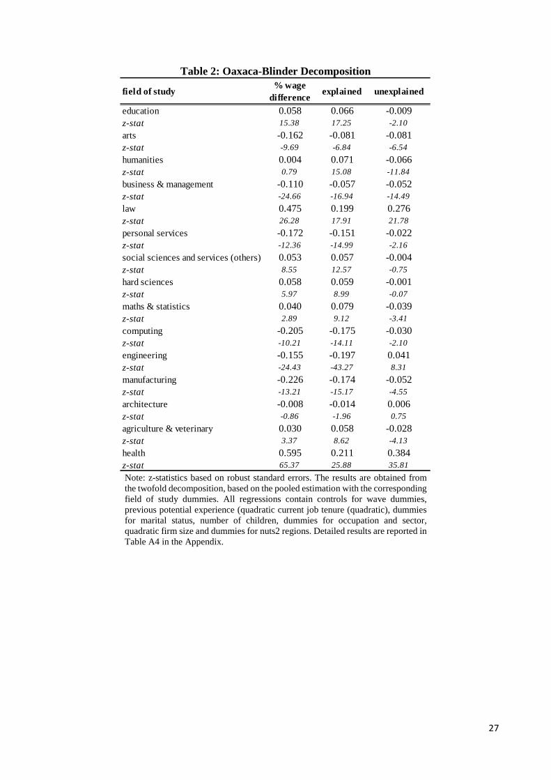
In order to better appreciate the role of observable characteristics and the associated

coefficients in accounting for the observed average wage gaps, we report the results from

the Oaxaca-Blinder decomposition shown in Equation (3). The basic results are displayed

in Table 2 and graphically illustrated in Figure 2. The detailed results that report the

contribution of each block of variables (and their returns) are shown in Table A4 in the

Appendix. It can be appreciated that the average wage gap in favor of graduates in

education (relative to other disciplines) is entirely explained by the endowment of

observable characteristics — mostly occupation. The lower average wages observed for

graduates in arts are similarly explained by the contribution of observed characteristics

and their return (both with a negative sign). Wages of graduates in humanities are around

the overall average and, for this field, the modest contribution of explained and

unexplained factors operate in opposite directions. The field of business & management

is less rewarded than others, which is almost equally explained by a less favorable

endowment of observable characteristics and lower returns. In contrast, for law (which is

15

a highly paid field) the unobservable components are slightly more relevant than the

observables in explaining the higher average hourly wage. For this field, the higher

coefficients associated with sector and occupation, and to a lesser extent their more

favorable composition in terms of these features of the job, represent the main driver of

the high and positive wage gap relative to other fields. The lower average remuneration

of graduates in personal services is almost entirely explained by observable

characteristics, whereby the effect of occupation prevails over the other covariates.

Observables are also responsible for the higher average wages in both social sciences and

hard sciences. For mathematics and statistics, the distribution of endowments positively

affects average hourly wages, but the returns to endowments operate in the opposite

direction. Average hourly pay is lower for graduates in computing, engineering, or

manufacturing than for graduates of other fields, and the observable characteristics seem

to account for almost their entire wage gaps. More specifically, for computing lower work

experience/job tenure are the main conditioning factors behind the negative wage

differential they suffer. For engineering, occupation is the most important observed factor

that accounts for the negative gap, followed by sector/firm size and work experience.

These three sets of observable characteristics are also the main driver of the wage penalty

experienced by graduates in manufacturing, with a similar weight. The wage rate for

graduates in architecture does not significantly differ from those in other fields, and the

slightly higher wages for agriculture & veterinary are driven by the net effect of a better

distribution of observed characteristics and lower associated returns. Finally, the field of

health is clearly better rewarded, whereby the unexplained factors are more important

than the explained. As in the case of law, the higher return to occupation (but not to

employment sector and firm size) is the main factor behind the premium for graduates in

health disciplines.

4.2) Differences along the Wage Distribution

Selected coefficients from RIF-Regressions estimated at different deciles of the

unconditional wage distribution are displayed in Table 3 (complete results are not shown

but are available upon request). These represent the estimates of equation (6), which are

obtained using the full set of control variables. We also report the result from the OLS

regression to allow for comparison. The same evidence can be graphically appreciated in

Figure 3. Overall, the results highlight substantial heterogeneity in wage differentials by

16

field of study along the distribution of real hourly wages. Relative to business &

management, graduates in education are better remunerated at the bottom of the

unconditional wage distribution, but the effect decreases monotonically with the quantiles

and becomes negative after the median. A similar pattern is observed for humanities. In

contrast, the high average reward to a degree in law that is detected by OLS is mostly

operating in the upper part of the wage distribution, since for lower deciles the positive

gap relative to the reference field is significantly less pronounced (but still positive).

Social science degrees yield a payoff relative to business & management only at the

bottom of the wage distribution, while no important differences are detected above the

median.

Interestingly, the wage premium in hard sciences is higher at lower quantiles, but

remains significant over the whole distribution. Graduates in mathematics & statistics are

instead slightly less rewarded than those in business & management only in the middle

of the distribution. As for graduates in computing, we observe lower wages at the left tail

of the distribution, but the sign of the gap is reversed above the median. Indeed, this

substantial heterogeneity was not captured by the average differential estimated by OLS,

which is virtually zero. Similarly, also for the field of manufacturing there is a negative

gap relative to business & management in the lower decile of the wage distribution, which

reverts to positive around the center. However, no significant differences are detected at

higher deciles. The returns to engineering increase along the unconditional wage

distribution, while the estimated differential decreases slightly for architecture. In any

case, both fields are better remunerated than business & management along the whole

unconditional distribution of hourly wages. Hourly pay gaps between agriculture &

veterinary and the reference field follow an inverted U-shaped pattern (being negative at

the lowest and highest deciles, respectively). Finally, similar to the case of law, the

positive wage gap in favor of health is especially high at the top of the unconditional wage

distribution, but is also relevant even at its left cue.

The decomposition results of wage gaps at different deciles of the unconditional

wage distribution are reported in Table 4 and graphically displayed in Figure 4. Detailed

RIF-decomposition results are shown in Table A6 in the Appendix. It appears that

observable and unobservable components have a similar weight in explaining wage

differences for the field of education at different points of the wage distribution and

follow the overall decreasing tendency of the wage gap relative to other fields. The

positive contribution of observable characteristics detected at lower deciles is mostly

17

driven by occupation, which exerts a positive effect over the entire distribution, but is

indeed compensated by the negative impact of sector and firm size above the median. The

lower returns to work experience and occupation appear to be the main drivers of the

decreasing contribution of unexplained factors, which is especially pronounced at the

bottom of the wage distribution. For the field of arts, the endowment of observable

characteristics plays an important role in accounting for the negative wage gap detected

at the bottom of the distribution, but tends to decrease along it. The negative contribution

of the estimated coefficients is also very pronounced at the second and third quantile,

being mostly driven by the return to family characteristics (which is also relevant at the

top of the distribution). Observable characteristics account for most of the positive wage

gap observed for humanities at the bottom of the wage distribution, but their relevance

declines and even becomes negative at top quantiles (where graduates in this field earn

less than their counterparts). Similar to the case of education, although occupational

selection represents a favorable endowment for graduates in humanities, differences in

employment sector and firm size penalize them at the top of the distribution. Also, the

lower returns to work experience and occupation substantially contribute to the sharp

decrease of the role of unobservables in accounting for the wage gap at bottom deciles.

In the case of business & management, the negative wage gap that graduates in this

field experience relative to their counterparts generally tends to vanish along the

unconditional wage distribution (with the exception of the last quantile) and seems to be

mostly driven by the unfavorable distribution of endowments at lower deciles. More

specifically, occupational selection tends to penalize low-paid graduates in this field.

Occupation seems to exert a negative effect on wages of graduates in business &

management also at the top of the distribution, but its effect is compensated by the

positive impact of sector and firm size. For law, returns and endowments operate in

opposite directions at different points of the wage distribution, since the effect of

explained factors decreases along the quantiles and the contribution of unexplained

elements increases and accounts for most of the remarkably positive wage gap graduates

in this field enjoy at the top of the wage distribution. Among the observables, employment

sector and firm size are especially beneficial for bottom deciles, while occupation shows

a relatively stable positive contribution over the entire wage distribution. Regarding the

unexplained factors, it seems worth highlighting the changing contribution of the return

to work experience, which exerts a negative impact at the bottom of the distribution and

reverts sign at the median. Moreover, return to occupational categories has a positive

18

impact at the center of the unconditional distribution and contributes to the high wage gap

experienced by graduates in law. The negative wage gap for personal service is largely

explained by the unfavorable endowment of observable characteristics, with the

exception of the left tail of the wage distribution where the contribution of unexplained

factors slightly mitigates the distribution of observables. Detailed decomposition results

show that occupational choices are the most important drivers of the negative effect of

endowments for personal services, being the contribution of this element that is especially

relevant at the bottom and the top of the unconditional distribution of wages. Graduates

in social sciences experience a positive wage gap at the bottom of the wage distribution,

which is mostly accounted by the positive contribution of observable characteristics (i.e.

work experience and sector/firm size). The importance of observables for this field

decreases along the wage distribution and is somewhat compensated by the slightly

negative impact of the estimated coefficients that is detected after the median.

The modest wage disparities between hard sciences and other fields, which tend to

be relatively constant over the entire distribution, seem to be mostly explained by the

effect of covariates, among which occupational selection plays the most important role.

Graduates in mathematics & statistics are better paid than their counterparts at the bottom

of the wage distribution, but this positive differential vanishes at its median. However, it

seems interesting to highlight that the positive (but decreasing) contribution of

observables is somewhat compensated by the estimated return, which tends to be lower

for graduates in this field. More specifically, occupation appears to be the most important

factor behind explained differences, whereas the returns to family characteristics and

sector/firm size display the most relevant contribution in accounting for the unexplained

wage gap. Graduates in computing are instead penalized with respect to graduates in other

fields, especially below the median of the unconditional wage distribution. The negative

differential detected at lower quantiles is mainly driven by observable factors, whereas

the corresponding coefficients play a most important role at the center of the distribution.

A similar pattern is detected for the fields of engineering and manufacturing, which are

less rewarded than other fields at the bottom of the distribution, but this negative wage

gap disappears when moving to higher quantiles (and even reverts sign in the case of

engineering). Indeed, for both fields the important negative differential detected in the

first half of the wage distribution is mostly explained by differences in observable

characteristics, being employment sector/firm size and, to a lesser extent, work

experience and occupation are the main observable factors behind these wage disparities.

19

Graduates in engineering and manufacturing obtain higher rewards to observable

characteristics at the bottom of the wage distribution, but the estimated coefficients tend

to penalize them around the central quantiles. Unexplained components have a positive

contribution for graduates in the former field above the median. Moreover, it seems

interesting to highlight the negative contribution of the coefficients associated to work

experience for the first two quantiles, which then reverts sign and tends to compensate

the lower returns to observables for these two technical fields of study. The field of

architecture is slightly less paid than others at the bottom of the distribution, while this

wage gap tends to revert above the median. In this case, explained and unexplained

components tend to operate in opposite directions along the unconditional wage

distribution, since the endowment of observable characteristics (mainly sector/firm size)

tend to penalize graduates in this field until the median, this differential being somewhat

compensated by slightly higher returns to characteristics (mostly sector/firm size and

occupation). For agriculture & veterinary, the inverted U-shaped contribution of

unexplained characteristics is what drives the same pattern observed for the overall wage

gap. Indeed, they tend to be better paid than other fields around the center of the wage

distribution and the endowment of observable characteristics is generally favorable for

them but the contribution of the estimated coefficients tend to be negative at the two

extremes of the distribution and positive in the middle. We detected a positive impact of

the coefficients associated with family characteristics along the whole distribution, as

well as of sector/firm size until the median, but these are compensated by the lower return

to work experience for graduates in agriculture & veterinary relative to their counterparts

from other fields. Finally, the positive wage gap in health disciplines is the result of the

net effect of the contrasting contribution of characteristics (with a decreasing weight

along the wage distribution) and coefficients (with an increasing weight at higher

quantiles), which is indeed a similar pattern observed for the case of law. Moreover,

among the observable characteristics, selection into occupation and employment sector

and, to a lesser extent, differences in work experience represent the main factors behind

the significant wage premium experienced by graduates in health disciplines.

20

5) Conclusions

This paper reports evidence on the pay disparities among tertiary educated workers

who hold a degree in different fields of study. We focus our analysis on Turkey, a

developing country that has been characterized by a sustained expansion of higher

education during the last decades. We detected significant heterogeneity in wage rates

across college majors, which are especially pronounced for the fields of law and health.

Indeed, graduates in these two disciplines are by far the better paid tertiary educated

(male) workers in the Turkish labor market. Observable characteristics matter in

explaining wage differences by field of study, since conditioning for characteristics alters

the magnitude and in some case also the sign of the estimated differentials. Consistent

with previous evidence in the literature, occupational selection represents the most

important driver of pay gaps, but also employment sector, firm size and work experience

operate as conditioning factors of the wages of Turkish university graduates. On the

contrary, other observable factors appear to be less relevant, such as family characteristics

(possibly because we focused on males) or geographical location (with the exception of

the field of agriculture & veterinary).

With the aim of appreciating the extent to which the observed wage gaps are driven

by differences in observable characteristics and/or by differences in the return associated

to those characteristics, we performed the Oaxaca-Blinder decomposition for average

wage differentials. The results indicate that differences in the endowments (i.e. the

explained component) account for a substantial share of the wage gaps, and even explain

almost the entire wage gap in some cases. Indeed, the overall effect of the return to

characteristics (i.e. the unexplained component) is negligible and even not significant for

several fields of study, such as social science and services, hard sciences and architecture

(while marginally significant for education and personal services). It seems also worth

noting that, in some cases, explained and unexplained components contribute to the wage

gaps in opposite directions. Finally, the contribution of unexplained elements turns out to

be especially high and actually higher than the contribution of observables for the two top

paid fields of study, law, and health. This finding is possibly due to the importance of

self-selection of high wage potential individuals into these two fields, which are among

the ones with the highest cut-off score requirements for the university admission test, but

also to labor market regulations that cover most of the jobs/sectors where graduates in

law and health are usually employed.

21

As long as important wage disparities between individuals who obtained a degree in

a different field of study could occur at other points of the distribution than the mean, we

investigated distributional wage gaps along the unconditional distribution of hourly

wages. Recentered Influence Function (RIF) Regressions estimates indicate that wage

disparities by college major generally vary over the wage distribution, making the

distributional analysis particularly relevant to analyze pay gaps by field of study. Indeed,

wage differences (relative to the reference category) display a decreasing pattern for the

fields of education, humanities, personal services, social services, mathematics &

statistics and architecture (except for the last quantile), moving from positive to negative

differentials. In contrast, pay disparities tend to increase along the wage distribution for

law, health, computing, and engineering (moving from negative to positive for the latter

two), and display an inverted U-shaped pattern for graduates in arts, manufacturing, and

agriculture & veterinary.

We finally decomposed distributional wage differentials, in order to understand

whether the contributions of explained and unexplained factors also change at different

points of the unconditional distribution of hourly wages. The distributional

decomposition confirms that the endowment of observable characteristics represents the

main driver of wage differentials, but their contribution to the observed wage gaps tends

to decrease when moving to the upper part of the unconditional wage distribution and

even changes sign after the median (changing from positive to negative for education,

humanities, and mathematics & statistics, and from negative to positive for architecture).

Unexplained elements instead appear very relevant for the fields of law and health, the

top paid college majors, and actually account for an increasingly important part of the

positive wage gap experienced by graduates in these two fields in the upper part of the

unconditional wage distribution.

Overall, the results point out that selection into occupation and, to a lesser extent,

into economic sectors represents the main mechanism behind observed wage differences

between individuals who obtained a university degree in a different field of study. As

long as these two selection mechanisms are likely to be determined by both observable

and unobservable individual characteristics (possibly correlated with wage potential), and

in this work we are unable to disentangle between the two, additional research is needed

to better understand the real contribution of occupation and employment sector to the

wage return attributed to different fields of study. Related to this, although the

contribution of unexplained factors is generally lower than the contribution of

22

observables, understanding the extent to which endogenous self-selection of individuals

into different fields of study represents the main driver of wage differences represents a

challenge for future research, which will be possible when more detailed (administrative)

data also becomes available in the case of Turkey. Indeed, it is quite likely that selection

into the fields of law and health, based on unobserved traits that correlate with earnings

potential, would account for most of the high wage premium attached to these fields at

the top of the distribution (which is mostly left unexplained).

References

Arcidiacono, P. (2004). Ability sorting and the returns to college major. Journal of Econometrics, 121(1), 343-375. Altonji, J. G., Blom, E., and Meghir, C. (2012). Heterogeneity in human capital investments: High school curriculum, college major, and careers. Annual Review of Economics, 4(1), 185-223. Altonji, J. G., Kahn, L. B., and Speer, J. D. (2014). Trends in Earnings Differentials across College Majors and the Changing Task Composition of Jobs. The American Economic Review, 104(5), 387-393. Altonji, J. G., Arcidiacono, P. and Maurel, A. (2016). “The Analysis of Field Choice in College and Graduate School: Determinants and Wage Effects”. In Handbook of the Economics of Education, Vol. 5 (pages 305-396), ed. By E. A. Hanushek, S. Machin and L. Woessmann. Amsterdam: Elsevier.

Ballarino, G., and Bratti, M. (2009). Field of study and university graduates' early employment outcomes in Italy during 1995–2004. Labour, 23(3), 421-457. Beffy, M., Fougere, D., and Maurel, A. (2012). Choosing the field of study in postsecondary education: Do expected earnings matter? Review of Economics and Statistics, 94(1), 334-347. Berger, M. (1988). Predicted future earnings and choice of college major. Industrial and Labor Relations Review, 41, 418-429. Bhattacharya, J. (2005). Specialty selection and lifetime returns to specialization. Journal of Human Resources, 40(1), 115-143. Bratti, M., Naylor, R. and Smith, J. (2008). Heterogeneities in the returns to degrees: Evidence from the British cohort study 1970, Bonn, Germany: Institute for the Study of Labor (IZA) Discussion Paper No. 1631.

23

Buonanno, P., and Pozzoli, D. (2009). Early labour market returns to college subject. Labour, 23(4), 559-588. Caner, A., and Okten, C. (2010). Risk and career choice: Evidence from Turkey. Economics of Education Review, 29(6), 1060-1075. Chevalier, A. (2011). Subject choice and earnings of UK graduates. Economics of Education Review, 30(6), 1187-1201. Finnie, R., and Frenette, M. (2003). Earning differences by major field of study: evidence from three cohorts of recent Canadian graduates. Economics of Education Review, 22(2), 179-192. Firpo, S., Fortin, N., and Lemieux, T. (2007). Decomposing wage distributions using recentered influence function regressions. University of British Columbia Working Paper (June). Firpo, S., Fortin, N. M. and Lemieux, T. (2009). Unconditional Quantile Regressions. Econometrica, 77(3), 953-973. Fortin, N., Lemieux, T., and Firpo, S. (2011). “Decomposition methods in economics”. In Handbook of Labor Economics, Vol. 4A (pages 1-102), ed. by O. Ashenfelter and D. Card. Amsterdam: Elsevier. Frisancho, V., Krishna, K., Lychagin, S., and Yavas, C. (2016). Better luck next time: Learning through retaking. Journal of Economic Behavior and Organization, 125, 120-135. Grave, B. S., and Goerlitz, K. (2012). Wage differentials by field of study–the case of German university graduates. Education Economics, 20(3), 284-302. Hamermesh, D. S., and Donald, S. G. (2008). The effect of college curriculum on earnings: An affinity identifier for non-ignorable non-response bias. Journal of Econometrics, 144(2), 479-491. Hastings, J. S., Neilson, C. A., and Zimmerman, S. D. (2013). Are some degrees worth more than others? Evidence from college admission cutoffs in Chile. National Bureau of Economic Research (NBER) Working Paper No. w19241. Kelly, E., O’Connell, P. J., and Smyth, E. (2010). The economic returns to field of study and competencies among higher education graduates in Ireland. Economics of Education Review, 29(4), 650-657. Ketel, N., Leuven, E., Oosterbeek, H., & van der Klaauw, B. (2016). The Returns to Medical School: Evidence from Admission Lotters. American Economic Journal: Applied Economics, 8(2), 225-254. Kinsler, J., and Pavan, R. (2015). The Specificity of General Human Capital: Evidence from College Major Choice. Journal of Labor Economics, 33(4), 933–972.

24

Kirkeboen, L., Leuven, E., and Mogstad, M. (2016). Field of Study, Earnings, and Self-Selection. The Quarterly Journal of Economics, 131(3), 1057-1111. Lemieux, T. (2014). Occupations, fields of study and returns to education. Canadian Journal of Economics/Revue Canadienne d'économique, 47(4), 1047–1077. Livanos, I., and Pouliakas, K. (2011). Wage returns to university disciplines in Greece: are Greek higher education degrees Trojan Horses? Education Economics, 19(4), 411-445. Long, M. C., Goldhaber, D., and Huntington-Klein, N. (2015). Do completed college majors respond to changes in wages? Economics of Education Review, 49, 1-14. Montmarquette, C., Cannings, K., and Mahseredjian, S. (2002). How do young people choose college majors? Economics of Education Review, 21(6), 543-556. Stinebrickner, R., and Stinebrickner, T. (2014). A major in science? Initial beliefs and final outcomes for college major and dropout. The Review of Economic Studies, 81, 426–72.

Tansel, A. (1994). Wage Employment, Earnings and Returns to Schooling for Men and Women in Turkey. Economics of Education Review, 13 (4): 305-320.

Tansel, A. (2001). “Self-Employment, Wage-Employment, and Returns to Schooling by Gender in Turkey”. In Labor and Human Capital in the Middle East: Studies of Markets and Household Behavior (pages 637-667), ed. by D. Salehi-Isfahani. Reading, UK: Ithaca Press.

Tansel, A. (2010). Changing Returns to Education for Men and Women in a Developing Country: Turkey, 1994-2005. Paper presented at the ESPE conference, June 18-21, 2008, London UK, ECOMOD conference, July 2-4, 2008, Berlin Germany, MEEA conference, March 20-23, 2009, Nice, France and ICE-TEA conference, September 1-3, 2010 Girne, Republic of Northern Cyprus.

United Nations Educational Scientific and Cultural Organization (UNESCO) (2016) The International Standard Classification of Education (ISCED) Fields of Education and Training 2013, Paris: UNESCO, Institute for Statistics. Walker, I., and Zhu, Y. (2011). Differences by degree: Evidence of the net financial rates of return to undergraduate study for England and Wales. Economics of Education Review, 30(6), 1177-1186. Webber, D. A. (2014). The lifetime earnings premia of different majors: Correcting for selection based on cognitive, noncognitive, and unobserved factors. Labour Economics, 28, 14-23.

25

Tables and Figures

Figure 1a: Kernel Density Estimate of (Log) Hourly Wage by Field of Study

Figure 1b : Kernel Density Estimate of (Log) Hourly Wage by Field of Study

0.5

11.

52

1 2 3 4 5

education humanities arts

business & management personal services law

social sciences and services (others)

0.5

11.

52

1 2 3 4 5

hard sciences maths & statistics computing

engineering manufacturing architecture

agriculture & veterinary health

26

Table 1: Selected OLS Estimates

Note: robust standard errors in parenthesis, *** significant at 1%, ** significant at 5%, *** significant at 10%. Regression in column (2) contains controls for wave dummies, previous potential experience (quadratic) and current job tenure (quadratic). Regression in column (3) includes dummies for marital status and the number of children as additional controls. Regression in column (4) includes dummies for sector and quadratic firm size. Regression in column (5) includes dummies for occupation. Regression in column (6) includes dummies for nuts2 regions. Complete estimates are reported in Table A2 in the Appendix.

(1) (2) (3) (4) (5) (6)

education 0.129*** 0.103*** 0.093*** 0.086*** 0.013** 0.020***(0.005) (0.004) (0.004) (0.005) (0.005) (0.005)

arts -0.079*** -0.034** -0.036** -0.016 -0.038*** -0.047***(0.017) (0.015) (0.014) (0.014) (0.013) (0.013)

humanities 0.085*** -0.011* -0.008 0.038*** -0.038*** -0.036***(0.007) (0.006) (0.006) (0.007) (0.007) (0.007)

business & management

law 0.550*** 0.503*** 0.498*** 0.445*** 0.310*** 0.309***(0.018) (0.017) (0.017) (0.015) (0.013) (0.013)

personal services -0.088*** -0.105*** -0.099*** -0.065*** -0.008 0.002 (0.014) (0.012) (0.012) (0.011) (0.010) (0.010)

social sciences and services (others) 0.129*** 0.064*** 0.067*** 0.059*** 0.032*** 0.029***(0.007) (0.006) (0.006) (0.006) (0.005) (0.005)

hard sciences 0.137*** 0.132*** 0.131*** 0.130*** 0.041*** 0.045***(0.010) (0.009) (0.009) (0.009) (0.008) (0.008)

maths & statistics 0.120*** 0.132*** 0.119*** 0.068*** -0.006 -0.009 (0.014) (0.013) (0.013) (0.012) (0.012) (0.012)

computing -0.121*** 0.058*** 0.058*** 0.053*** 0.017 0.008 (0.020) (0.019) (0.019) (0.017) (0.015) (0.014)

engineering -0.052*** 0.007 0.007 0.051*** 0.062*** 0.067***(0.007) (0.006) (0.006) (0.006) (0.006) (0.006)

manufacturing -0.141*** -0.075*** -0.077*** -0.005 -0.028** -0.011 (0.017) (0.015) (0.015) (0.014) (0.012) (0.012)

architecture 0.073*** 0.082*** 0.087*** 0.094*** 0.034*** 0.044***(0.010) (0.010) (0.009) (0.009) (0.008) (0.008)

agriculture & veterinary 0.110*** 0.071*** 0.070*** 0.075*** -0.001 0.023***(0.010) (0.008) (0.008) (0.008) (0.007) (0.007)

health 0.646*** 0.580*** 0.574*** 0.531*** 0.405*** 0.410***(0.010) (0.009) (0.009) (0.012) (0.011) (0.011)

basic controls no yes yes yes yes yesfamily characteristics no no yes yes yes yessector dummies and firm size (sq.) no no no yes yes yesoccupation dummies no no no no yes yesnuts2 regions dummies no no no no no yesadjusted R-squared 0.091 0.263 0.283 0.361 0.472 0.489 number of observations 77154 77154 77154 77154 77154 77154

reference category

27

Table 2: Oaxaca-Blinder Decomposition

Note: z-statistics based on robust standard errors. The results are obtained from the twofold decomposition, based on the pooled estimation with the corresponding field of study dummies. All regressions contain controls for wave dummies, previous potential experience (quadratic current job tenure (quadratic), dummies for marital status, number of children, dummies for occupation and sector, quadratic firm size and dummies for nuts2 regions. Detailed results are reported in Table A4 in the Appendix.

field of study % wage difference explained unexplained

education 0.058 0.066 -0.009z-stat 15.38 17.25 -2.10arts -0.162 -0.081 -0.081z-stat -9.69 -6.84 -6.54humanities 0.004 0.071 -0.066z-stat 0.79 15.08 -11.84business & management -0.110 -0.057 -0.052z-stat -24.66 -16.94 -14.49law 0.475 0.199 0.276z-stat 26.28 17.91 21.78personal services -0.172 -0.151 -0.022z-stat -12.36 -14.99 -2.16social sciences and services (others) 0.053 0.057 -0.004z-stat 8.55 12.57 -0.75hard sciences 0.058 0.059 -0.001z-stat 5.97 8.99 -0.07maths & statistics 0.040 0.079 -0.039z-stat 2.89 9.12 -3.41computing -0.205 -0.175 -0.030z-stat -10.21 -14.11 -2.10engineering -0.155 -0.197 0.041z-stat -24.43 -43.27 8.31manufacturing -0.226 -0.174 -0.052z-stat -13.21 -15.17 -4.55architecture -0.008 -0.014 0.006z-stat -0.86 -1.96 0.75agriculture & veterinary 0.030 0.058 -0.028z-stat 3.37 8.62 -4.13health 0.595 0.211 0.384z-stat 65.37 25.88 35.81

28

Figure 2: Oaxaca-Blinder Decomposition

-.2 -.1 0 .1 .2 .3 .4 .5 .6

health

agriculture & veterinary

architecture

manufacturing

engineering

computing

maths & statistics

hard sciences

social sciences and serv.

personal services

law

business & management

humanities

arts

education

% wage difference explained unexplained

29

Table 3: Selected RIF-Regression Estimates

Note: robust standard errors in parenthesis, *** significant at 1%, ** significant at 5%, *** significant at 10%. All regressions contain controls for wave dummies, previous potential experience (quadratic), current job tenure (quadratic), dummies for marital status, number of children, dummies for occupation and sector, quadratic firm size and dummies for nuts2 regions.

OLS q1 q2 q3 q4 q5 q6 q7 q8 q9education 0.020*** 0.151*** 0.184*** 0.097*** 0.047*** 0.010* -0.012** -0.049*** -0.108*** -0.148***

(0.005) (0.014) (0.015) (0.009) (0.006) (0.006) (0.006) (0.006) (0.007) (0.011) arts -0.047*** -0.045 -0.117*** -0.054*** -0.016 -0.010 -0.009 -0.018 -0.040*** -0.069***

(0.013) (0.039) (0.039) (0.020) (0.014) (0.012) (0.012) (0.012) (0.015) (0.027) humanities -0.036*** 0.060*** 0.051*** 0.008 -0.031*** -0.057*** -0.067*** -0.076*** -0.084*** -0.133***

(0.007) (0.017) (0.018) (0.011) (0.009) (0.007) (0.007) (0.007) (0.008) (0.014) business & management

law 0.309*** 0.059** 0.098*** 0.089*** 0.090*** 0.106*** 0.149*** 0.205*** 0.372*** 1.087***(0.013) (0.023) (0.028) (0.017) (0.013) (0.011) (0.011) (0.012) (0.018) (0.049)

personal services 0.002 0.062* 0.031 -0.007 -0.001 -0.007 0.000 -0.002 -0.018 -0.054***(0.010) (0.033) (0.031) (0.017) (0.012) (0.010) (0.010) (0.010) (0.012) (0.018)

social sciences and services (others) 0.029*** 0.064*** 0.083*** 0.047*** 0.023*** 0.014*** 0.007 -0.004 0.003 0.022* (0.005) (0.013) (0.014) (0.009) (0.006) (0.005) (0.005) (0.005) (0.007) (0.013)

hard sciences 0.045*** 0.096*** 0.058*** 0.018 0.027*** 0.035*** 0.045*** 0.040*** 0.028*** 0.044** (0.008) (0.020) (0.022) (0.012) (0.009) (0.007) (0.007) (0.008) (0.010) (0.020)

maths & statistics -0.009 0.043 0.004 -0.043** -0.033** -0.025** -0.021* -0.031** -0.033** 0.032 (0.012) (0.028) (0.034) (0.020) (0.014) (0.012) (0.012) (0.012) (0.015) (0.028)

computing 0.008 -0.112*** -0.127*** -0.043** 0.006 0.021* 0.032*** 0.044*** 0.058*** 0.109***(0.014) (0.043) (0.040) (0.020) (0.013) (0.011) (0.010) (0.011) (0.014) (0.030)

engineering 0.067*** 0.031** 0.053*** 0.050*** 0.060*** 0.059*** 0.063*** 0.068*** 0.076*** 0.122***(0.006) (0.016) (0.016) (0.008) (0.006) (0.005) (0.005) (0.005) (0.006) (0.012)

manufacturing -0.011 -0.125*** -0.038 -0.017 0.019 0.037*** 0.039*** 0.031*** 0.020 -0.001 (0.012) (0.037) (0.034) (0.018) (0.012) (0.010) (0.010) (0.010) (0.013) (0.024)

architecture 0.044*** 0.047** 0.100*** 0.062*** 0.061*** 0.055*** 0.054*** 0.051*** 0.037*** 0.012 (0.008) (0.022) (0.023) (0.013) (0.009) (0.008) (0.007) (0.008) (0.010) (0.018)

agriculture & veterinary 0.023*** -0.017 0.014 0.044*** 0.063*** 0.064*** 0.076*** 0.075*** 0.044*** -0.055***(0.007) (0.019) (0.020) (0.011) (0.008) (0.007) (0.007) (0.008) (0.010) (0.017)

health 0.410*** 0.132*** 0.239*** 0.201*** 0.189*** 0.197*** 0.237*** 0.285*** 0.473*** 1.184***(0.011) (0.020) (0.024) (0.014) (0.011) (0.009) (0.009) (0.010) (0.014) (0.030)

R-squared 0.489 0.267 0.401 0.404 0.364 0.324 0.300 0.284 0.272 0.250number of observations 77154 77154 77154 77154 77154 77154 77154 77154 77154 77154

reference category

30

Figure 3: Selected RIF-Regression Estimates

Note: continuous lines represent the OLS estimates (as in the first column of Table 3) and dashed lines are the RIF-Regression estimates for different quantiles (as in the corresponding columns of Table 3).

-.2-.1

0.1

.2

1 2 3 4 5 6 7 8 9

education

-.15

-.1-.0

50

1 2 3 4 5 6 7 8 9

arts

-.15

-.1-.0

50

.05

1 2 3 4 5 6 7 8 9

humanities

0.2

.4.6

.81

1 2 3 4 5 6 7 8 9

law

-.05

0.0

5

1 2 3 4 5 6 7 8 9

personal services

0.0

2.0

4.0

6.0

8

1 2 3 4 5 6 7 8 9

social sciences and services (others)

.02

.04

.06

.08

.1

1 2 3 4 5 6 7 8 9

hard sciences

-.04

-.02

0.0

2.0

41 2 3 4 5 6 7 8 9

maths & statistics

-.15

-.1-.0

50

.05

.1

1 2 3 4 5 6 7 8 9

computing

.02

.04

.06

.08

.1.1

2

1 2 3 4 5 6 7 8 9

engineering-.1

5-.1

-.05

0.0

5

1 2 3 4 5 6 7 8 9

manufacturing

.02

.04

.06

.08

.1

1 2 3 4 5 6 7 8 9

architecture

-.05

0.0

5.1

1 2 3 4 5 6 7 8 9

agriculture & veterinary

.2.4

.6.8

11.

2

1 2 3 4 5 6 7 8 9

health

31

Table 4: RIF-Regression Decomposition

Note: z-statistics based on robust standard errors. The results are obtained from the twofold decomposition (computed at each decile of the RIF), based on the pooled estimation with the corresponding field of study dummies. All regressions contain controls for wave dummies, previous potential experience (quadratic), current job tenure (quadratic), dummies for marital status, number of children, dummies for occupation and sector, quadratic firm size and dummies for nuts2 regions.

q1 q2 q3 q4 q5 q6 q7 q8 q9

% wage difference 0.483 0.406 0.214 0.133 0.055 0.009 -0.037 -0.130 -0.286z-stat 30.93 62.04 45.91 36.61 17.33 2.78 -12.01 -37.79 -52.27explained 0.287 0.219 0.186 0.134 0.088 0.048 -0.004 -0.055 -0.156z-stat 27.95 26.57 31.16 30.46 23.42 12.80 -1.14 -12.92 -21.84unexplained 0.196 0.187 0.028 -0.002 -0.033 -0.039 -0.033 -0.075 -0.130z-stat 10.69 22.66 4.69 -0.34 -7.77 -9.08 -7.41 -15.08 -16.50

% wage difference -0.138 -0.293 -0.317 -0.229 -0.133 -0.088 -0.079 -0.082 -0.082z-stat -5.73 -10.37 -9.85 -6.49 -5.93 -5.33 -5.40 -5.12 -2.97explained -0.138 -0.237 -0.143 -0.092 -0.067 -0.051 -0.040 -0.027 0.007z-stat -6.59 -8.44 -8.85 -8.39 -8.11 -6.97 -5.70 -3.30 0.54unexplained 0.000 -0.056 -0.174 -0.137 -0.066 -0.037 -0.040 -0.055 -0.089z-stat 0.01 -2.07 -6.81 -4.70 -3.53 -2.59 -2.96 -3.63 -3.35

% wage difference 0.398 0.260 0.094 0.030 -0.022 -0.062 -0.103 -0.135 -0.204z-stat 21.84 28.49 15.19 6.08 -4.94 -14.29 -21.65 -20.89 -21.70explained 0.259 0.347 0.208 0.107 0.047 -0.006 -0.041 -0.077 -0.139z-stat 27.58 31.61 28.60 20.36 11.06 -1.56 -10.99 -17.71 -19.04unexplained 0.139 -0.088 -0.114 -0.076 -0.069 -0.057 -0.063 -0.058 -0.065z-stat 7.64 -8.10 -15.50 -13.61 -14.13 -11.97 -12.10 -8.08 -5.86

% wage difference -0.128 -0.194 -0.155 -0.115 -0.084 -0.067 -0.036 -0.054 -0.133z-stat -14.67 -18.07 -20.06 -23.48 -19.56 -17.06 -8.85 -12.05 -18.91explained -0.108 -0.132 -0.088 -0.060 -0.041 -0.027 -0.016 -0.009 -0.034z-stat -17.17 -16.85 -18.04 -18.88 -15.28 -10.86 -6.54 -3.28 -6.83unexplained -0.020 -0.062 -0.067 -0.055 -0.043 -0.041 -0.020 -0.044 -0.099z-stat -2.23 -6.49 -10.33 -13.07 -11.58 -11.51 -5.36 -10.25 -13.41

% wage difference 0.554 0.407 0.322 0.345 0.425 0.499 0.563 0.688 0.665z-stat 16.32 18.35 12.62 13.46 16.06 21.56 18.88 24.32 54.16explained 0.281 0.420 0.250 0.176 0.148 0.147 0.155 0.168 0.160z-stat 14.77 15.76 16.64 17.11 18.53 20.26 20.83 20.30 12.00unexplained 0.273 -0.013 0.072 0.170 0.277 0.352 0.408 0.521 0.505z-stat 9.05 -0.55 3.41 8.09 12.22 17.60 15.37 20.10 30.98

% wage difference -0.163 -0.258 -0.222 -0.159 -0.138 -0.124 -0.108 -0.115 -0.181z-stat -7.12 -7.07 -6.99 -8.62 -8.96 -9.05 -8.05 -9.00 -13.44explained -0.261 -0.293 -0.180 -0.126 -0.099 -0.085 -0.079 -0.091 -0.148z-stat -14.14 -11.81 -12.59 -13.63 -13.66 -13.09 -12.49 -12.77 -13.28unexplained 0.098 0.035 -0.042 -0.032 -0.039 -0.038 -0.030 -0.025 -0.033z-stat 4.42 1.19 -1.72 -2.27 -3.13 -3.30 -2.49 -2.03 -2.28

% wage difference 0.169 0.171 0.059 0.030 0.007 0.005 0.006 0.032 0.025z-stat 8.95 14.77 8.40 5.06 1.36 0.98 1.08 4.65 1.89explained 0.101 0.141 0.062 0.032 0.023 0.025 0.037 0.046 0.048z-stat 13.47 14.24 10.32 7.61 7.00 7.78 11.40 12.38 7.77unexplained 0.068 0.030 -0.002 -0.001 -0.016 -0.020 -0.030 -0.014 -0.024z-stat 3.96 2.92 -0.38 -0.28 -3.37 -4.17 -5.80 -2.17 -1.95

business & management

law

personal services

social sciences and services (others)

humanities

education

arts

32

Table 4 (continued): RIF-Regression Decomposition

Note: z-statistics based on robust standard errors. The results are obtained from the twofold decomposition (computed at each decile of the RIF), based on the pooled estimation with the corresponding field of study dummies. All regressions contain controls for wave dummies, previous potential experience (quadratic), current job tenure (quadratic), dummies for marital status, number of children, dummies for occupation and sector, quadratic firm size and dummies for nuts2 regions.

q1 q2 q3 q4 q5 q6 q7 q8 q9

% wage difference 0.077 0.043 0.036 0.052 0.070 0.067 0.049 0.051 0.088z-stat 3.65 1.95 2.24 4.71 8.04 8.61 6.18 5.09 4.26explained 0.050 0.066 0.058 0.056 0.052 0.051 0.048 0.055 0.094z-stat 4.66 4.33 6.53 9.18 11.21 12.29 11.39 11.18 11.26unexplained 0.028 -0.023 -0.023 -0.004 0.018 0.016 0.002 -0.004 -0.006z-stat 1.44 -1.24 -1.77 -0.42 2.49 2.36 0.25 -0.40 -0.32

% wage difference 0.204 0.131 0.058 0.044 0.013 0.006 -0.011 -0.032 0.002z-stat 4.23 4.61 3.25 3.29 1.18 0.55 -0.97 -2.16 0.05explained 0.170 0.258 0.167 0.108 0.072 0.047 0.018 -0.013 -0.042z-stat 12.56 13.86 15.11 13.93 11.59 7.99 2.96 -1.73 -3.22unexplained 0.034 -0.127 -0.108 -0.064 -0.059 -0.041 -0.029 -0.018 0.043z-stat 0.75 -4.82 -6.71 -5.32 -5.66 -4.27 -2.88 -1.39 1.46

% wage difference -0.235 -0.437 -0.484 -0.408 -0.278 -0.180 -0.091 -0.019 0.071z-stat -11.00 -18.68 -17.90 -12.91 -8.57 -6.71 -3.39 -0.80 1.73explained -0.321 -0.512 -0.305 -0.194 -0.131 -0.096 -0.070 -0.037 0.006z-stat -15.36 -19.33 -20.37 -18.95 -15.51 -12.06 -8.64 -3.85 0.38unexplained 0.087 0.075 -0.180 -0.214 -0.147 -0.084 -0.021 0.018 0.065z-stat 3.62 2.91 -8.12 -8.04 -5.23 -3.72 -0.91 0.92 1.75

% wage difference -0.221 -0.416 -0.409 -0.288 -0.156 -0.082 -0.018 0.020 0.059z-stat -24.43 -41.46 -40.63 -26.09 -16.82 -11.40 -2.72 2.79 5.33explained -0.388 -0.481 -0.296 -0.235 -0.174 -0.116 -0.082 -0.053 -0.032z-stat -37.76 -50.53 -50.71 -46.39 -41.82 -33.80 -25.12 -14.49 -5.27unexplained 0.167 0.065 -0.112 -0.052 0.018 0.034 0.064 0.072 0.090z-stat 13.49 6.22 -13.69 -5.79 2.28 5.36 10.59 10.78 8.12

% wage difference -0.280 -0.439 -0.467 -0.350 -0.235 -0.127 -0.059 -0.062 -0.078z-stat -14.55 -18.61 -14.79 -11.08 -9.29 -5.23 -3.63 -3.94 -3.48explained -0.322 -0.503 -0.293 -0.178 -0.122 -0.091 -0.059 -0.042 -0.022z-stat -16.21 -19.60 -19.78 -17.87 -15.59 -12.70 -8.66 -5.30 -1.80unexplained 0.042 0.064 -0.174 -0.172 -0.113 -0.036 0.001 -0.020 -0.056z-stat 1.96 2.73 -7.00 -6.68 -5.43 -1.76 0.04 -1.41 -2.59

% wage difference -0.029 -0.040 -0.051 -0.008 0.006 0.035 0.049 0.037 -0.005z-stat -1.34 -1.69 -2.90 -0.69 0.53 3.89 5.72 4.02 -0.36explained -0.028 -0.100 -0.072 -0.038 -0.018 0.003 0.019 0.039 0.049z-stat -2.06 -5.61 -7.14 -5.79 -3.41 0.59 4.06 7.21 5.41unexplained -0.001 0.060 0.020 0.030 0.023 0.033 0.030 -0.003 -0.054z-stat -0.05 2.87 1.38 2.97 2.60 4.11 3.88 -0.29 -3.95

% wage difference 0.013 0.072 0.067 0.086 0.093 0.092 0.061 0.047 -0.050z-stat 0.53 2.98 4.64 8.35 11.24 13.32 9.00 6.58 -5.41explained 0.073 0.111 0.061 0.046 0.043 0.046 0.051 0.061 0.066z-stat 6.31 6.92 6.74 7.46 9.10 10.77 11.77 12.56 8.09unexplained -0.060 -0.039 0.006 0.040 0.050 0.046 0.011 -0.014 -0.116z-stat -2.83 -2.04 0.51 4.74 7.13 7.55 1.72 -1.92 -10.31

% wage difference 0.730 0.554 0.406 0.420 0.501 0.617 0.710 0.758 0.791z-stat 48.88 54.83 41.93 29.48 32.65 44.44 59.27 68.44 65.56explained 0.303 0.387 0.259 0.230 0.207 0.165 0.127 0.102 0.107z-stat 17.96 19.51 19.95 21.85 21.78 19.45 16.56 13.28 10.31unexplained 0.427 0.167 0.147 0.190 0.294 0.452 0.583 0.657 0.685z-stat 19.60 7.99 9.71 11.49 17.72 30.58 45.61 54.94 47.36

health

maths & statistics

computing

engineering

manufacturing

architecture

agriculture & veterinary

hard sciences

33

Figure 4: RIF-Regression Decomposition

-.4-.2

0.2

.4

1 2 3 4 5 6 7 8 9

education

-.3-.2

-.10

1 2 3 4 5 6 7 8 9

arts

-.20

.2.4

1 2 3 4 5 6 7 8 9

humanities

-.2-.1

5-.1

-.05

0

1 2 3 4 5 6 7 8 9

business & management

0.2

.4.6

.8

1 2 3 4 5 6 7 8 9

law

-.3-.2

-.10

.1

1 2 3 4 5 6 7 8 9

personal services

-.05

0.0

5.1

.15

1 2 3 4 5 6 7 8 9

social sciences and services (others)

-.05

0.0

5.1

1 2 3 4 5 6 7 8 9

hard sciences

-.10

.1.2

.3

1 2 3 4 5 6 7 8 9

maths & statistics

-.6-.4

-.20

.2

1 2 3 4 5 6 7 8 9

computing

-.6-.4

-.20

.2

1 2 3 4 5 6 7 8 9

engineering

-.6-.4

-.20

.21 2 3 4 5 6 7 8 9

manufacturing

-.1-.0

50

.05

1 2 3 4 5 6 7 8 9

architecture

-.1-.0

50

.05

.1

1 2 3 4 5 6 7 8 9

agriculture & veterinary0

.2.4

.6.8

1 2 3 4 5 6 7 8 9

health

wage differential explained unexplained

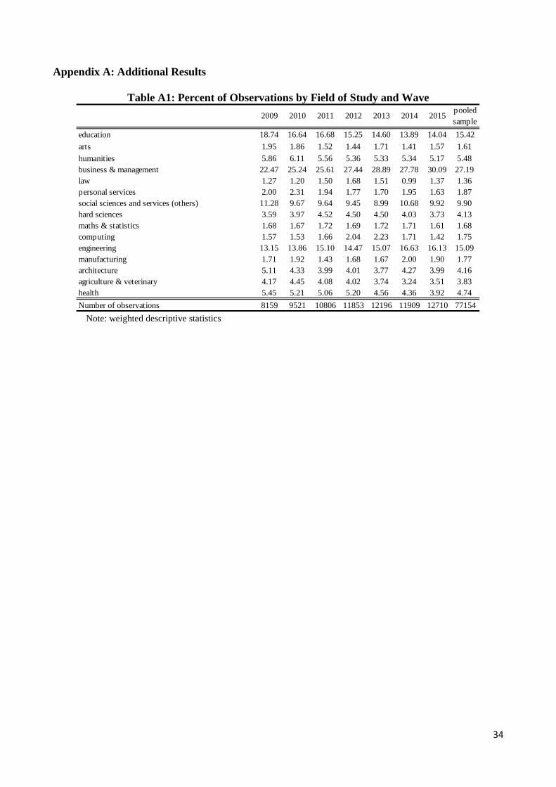
34

Appendix A: Additional Results

Table A1: Percent of Observations by Field of Study and Wave

Note: weighted descriptive statistics

education 18.74 16.64 16.68 15.25 14.60 13.89 14.04 15.42arts 1.95 1.86 1.52 1.44 1.71 1.41 1.57 1.61 humanities 5.86 6.11 5.56 5.36 5.33 5.34 5.17 5.48 business & management 22.47 25.24 25.61 27.44 28.89 27.78 30.09 27.19 law 1.27 1.20 1.50 1.68 1.51 0.99 1.37 1.36 personal services 2.00 2.31 1.94 1.77 1.70 1.95 1.63 1.87 social sciences and services (others) 11.28 9.67 9.64 9.45 8.99 10.68 9.92 9.90 hard sciences 3.59 3.97 4.52 4.50 4.50 4.03 3.73 4.13 maths & statistics 1.68 1.67 1.72 1.69 1.72 1.71 1.61 1.68 computing 1.57 1.53 1.66 2.04 2.23 1.71 1.42 1.75 engineering 13.15 13.86 15.10 14.47 15.07 16.63 16.13 15.09 manufacturing 1.71 1.92 1.43 1.68 1.67 2.00 1.90 1.77 architecture 5.11 4.33 3.99 4.01 3.77 4.27 3.99 4.16 agriculture & veterinary 4.17 4.45 4.08 4.02 3.74 3.24 3.51 3.83 health 5.45 5.21 5.06 5.20 4.56 4.36 3.92 4.74 Number of observations 8159 9521 10806 11853 12196 11909 12710 77154

2009 2010 2011 2012 2013 2014 2015pooled sample

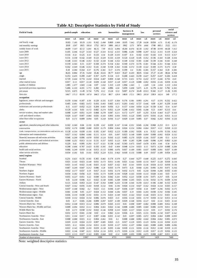
35

Table A2: Descriptive Statistics by Field of Study

Note: weighted descriptive statistics

mean s.d. mean s.d. mean s.d. mean s.d. mean s.d. mean s.d. mean s.d. mean s.d.real hourly wage 10.83 7.185 10.19 3.355 9.162 5.498 9.869 3.909 10.05 7.042 17.28 9.638 8.834 4.73 11.42 8.179real monthly earnings 2018 1297 1815 583.8 1752 997.9 1800 663.3 1902 1273 3074 1666 1748 883.1 2122 1511weekly hours of work 44.89 7.547 42.12 5.691 46.15 7.99 43.51 6.896 45.84 8.076 42.18 5.592 47.98 8.978 44.58 7.412wave 2009 0.105 0.306 0.127 0.333 0.127 0.333 0.112 0.315 0.086 0.281 0.098 0.297 0.112 0.315 0.119 0.324wave 2010 0.116 0.32 0.125 0.33 0.133 0.34 0.129 0.335 0.107 0.31 0.102 0.303 0.143 0.35 0.113 0.317wave 2011 0.131 0.338 0.142 0.349 0.123 0.329 0.133 0.339 0.124 0.329 0.145 0.352 0.136 0.343 0.128 0.334wave 2012 0.148 0.355 0.146 0.353 0.132 0.338 0.144 0.352 0.149 0.356 0.181 0.386 0.139 0.346 0.141 0.348wave 2013 0.159 0.365 0.15 0.357 0.169 0.374 0.154 0.361 0.169 0.374 0.176 0.381 0.144 0.351 0.144 0.351wave 2014 0.162 0.369 0.146 0.353 0.141 0.348 0.158 0.365 0.166 0.372 0.118 0.322 0.169 0.375 0.175 0.38wave 2015 0.18 0.384 0.164 0.37 0.176 0.381 0.17 0.376 0.199 0.4 0.181 0.385 0.157 0.364 0.18 0.385age 36.65 8.884 37.35 9.458 35.46 8.616 39.77 8.825 35.67 8.203 38.05 9.566 37.27 8.149 38.64 8.784single 0.253 0.435 0.209 0.407 0.357 0.479 0.124 0.33 0.268 0.443 0.239 0.427 0.257 0.437 0.226 0.418married 0.729 0.444 0.774 0.418 0.614 0.487 0.859 0.348 0.715 0.451 0.753 0.432 0.727 0.446 0.755 0.43other marital status 0.017 0.13 0.017 0.128 0.029 0.168 0.017 0.128 0.017 0.129 0.008 0.092 0.016 0.126 0.019 0.136number of children 1.085 1.077 1.043 1.146 0.97 1.032 1.313 1.229 1.094 1.043 1 1.049 1.14 1.034 1.113 1.054(potential) previous experience 5.406 6.103 4.101 5.772 6.282 5.84 4.896 6.04 5.059 5.698 5.671 6.29 6.178 6.182 5.782 6.365job tenure 9.515 8.875 11.49 9.734 7.276 8.12 13.24 9.53 9.007 8.274 10.49 8.913 9.342 9.127 11.26 9.395firm size 144.7 171.3 83.95 107.8 144.5 172.6 80.7 129.9 148.8 172.1 190.5 205.8 138.9 162.6 149 177.2occupationlegislators, senior officials and managers 0.159 0.366 0.187 0.39 0.129 0.335 0.157 0.364 0.176 0.381 0.093 0.291 0.17 0.376 0.232 0.422professionals 0.405 0.491 0.665 0.472 0.416 0.493 0.665 0.472 0.203 0.402 0.727 0.446 0.09 0.287 0.259 0.438technicians and associate professionals 0.15 0.357 0.052 0.221 0.204 0.403 0.056 0.23 0.157 0.364 0.054 0.226 0.158 0.365 0.14 0.347clerks 0.129 0.335 0.03 0.172 0.082 0.274 0.055 0.229 0.248 0.432 0.045 0.208 0.21 0.407 0.213 0.41service workers, shop and market sales 0.098 0.297 0.051 0.219 0.084 0.278 0.047 0.211 0.172 0.377 0.07 0.255 0.314 0.464 0.127 0.333craft and related workers 0.029 0.167 0.007 0.084 0.035 0.183 0.003 0.056 0.015 0.124 0.005 0.074 0.016 0.126 0.013 0.113other blue-collar occupations 0.03 0.171 0.009 0.094 0.05 0.218 0.016 0.127 0.029 0.169 0.005 0.07 0.042 0.202 0.016 0.126sectoragriculture, manufacturing and other industries 0.162 0.369 0.04 0.195 0.228 0.42 0.029 0.167 0.144 0.351 0.045 0.206 0.068 0.253 0.11 0.313construction 0.032 0.176 0.008 0.088 0.033 0.179 0.004 0.064 0.024 0.154 0.004 0.064 0.017 0.13 0.018 0.133trade, transportation, accommodation and service act. 0.128 0.334 0.039 0.193 0.105 0.307 0.052 0.223 0.189 0.392 0.026 0.16 0.352 0.478 0.156 0.362information and communication 0.027 0.162 0.004 0.066 0.111 0.314 0.01 0.097 0.023 0.148 0.009 0.094 0.008 0.092 0.024 0.152financial, insurance ad real estate activities 0.046 0.209 0.006 0.078 0.016 0.124 0.016 0.125 0.085 0.279 0.029 0.166 0.037 0.189 0.11 0.314professional, scientific and technical activities 0.068 0.251 0.013 0.114 0.131 0.337 0.015 0.123 0.09 0.285 0.208 0.406 0.096 0.295 0.063 0.243public administration and defense 0.229 0.42 0.095 0.293 0.117 0.321 0.138 0.345 0.343 0.475 0.647 0.478 0.303 0.46 0.34 0.474education 0.208 0.406 0.767 0.423 0.193 0.395 0.42 0.494 0.048 0.214 0.023 0.15 0.073 0.259 0.088 0.284health and social services 0.066 0.249 0.019 0.136 0.013 0.115 0.006 0.076 0.037 0.189 0.001 0.037 0.008 0.091 0.037 0.189other service activities 0.034 0.181 0.01 0.101 0.053 0.224 0.311 0.463 0.018 0.135 0.008 0.09 0.037 0.189 0.054 0.225nuts2 regionsIstanbul 0.231 0.421 0.135 0.341 0.365 0.482 0.174 0.379 0.27 0.444 0.277 0.448 0.225 0.417 0.272 0.445Thrace 0.021 0.143 0.023 0.149 0.031 0.173 0.011 0.106 0.021 0.142 0.018 0.133 0.017 0.128 0.018 0.134Southern Marmara - West 0.021 0.145 0.022 0.146 0.021 0.142 0.027 0.162 0.02 0.141 0.019 0.136 0.024 0.153 0.019 0.136Izmir 0.067 0.249 0.047 0.212 0.086 0.28 0.033 0.179 0.073 0.26 0.044 0.205 0.095 0.293 0.071 0.256Southern Aegean 0.032 0.177 0.037 0.19 0.017 0.131 0.031 0.174 0.032 0.175 0.05 0.218 0.044 0.206 0.035 0.183Northern Aegean 0.034 0.182 0.056 0.23 0.031 0.173 0.039 0.194 0.028 0.165 0.018 0.133 0.028 0.165 0.03 0.171Eastern Marmara - South 0.055 0.227 0.051 0.22 0.049 0.216 0.042 0.201 0.052 0.221 0.038 0.191 0.071 0.257 0.05 0.218Eastern Marmara - North 0.05 0.218 0.046 0.21 0.022 0.148 0.045 0.208 0.044 0.205 0.025 0.156 0.032 0.176 0.039 0.194Ankara 0.121 0.326 0.053 0.224 0.147 0.354 0.069 0.253 0.139 0.346 0.218 0.413 0.106 0.308 0.152 0.359Central Anatolia - West and South 0.027 0.162 0.035 0.183 0.018 0.132 0.04 0.196 0.024 0.154 0.027 0.162 0.024 0.154 0.025 0.157Mediterranean region - West 0.037 0.188 0.042 0.2 0.023 0.15 0.036 0.187 0.036 0.187 0.034 0.18 0.097 0.296 0.032 0.175Mediterranean region - Middle 0.041 0.198 0.05 0.217 0.024 0.153 0.044 0.206 0.037 0.19 0.043 0.203 0.038 0.192 0.036 0.185Mediterranean region - East 0.026 0.159 0.038 0.191 0.031 0.174 0.023 0.149 0.021 0.142 0.022 0.146 0.023 0.151 0.021 0.143Central Anatolia - Middle 0.018 0.132 0.024 0.154 0.006 0.076 0.023 0.15 0.016 0.126 0.031 0.174 0.018 0.132 0.013 0.114Central Anatolia - East 0.03 0.17 0.045 0.206 0.009 0.097 0.037 0.189 0.029 0.168 0.016 0.127 0.02 0.141 0.021 0.143Western Black Sea - West 0.012 0.108 0.013 0.112 0.006 0.079 0.025 0.155 0.01 0.098 0.007 0.082 0.008 0.089 0.012 0.108Western Black Sea - Middle and East 0.009 0.094 0.012 0.111 0.004 0.065 0.022 0.146 0.008 0.089 0.005 0.069 0.006 0.078 0.011 0.102Middle Black Sea 0.03 0.171 0.038 0.192 0.022 0.146 0.058 0.233 0.025 0.157 0.024 0.153 0.03 0.17 0.032 0.176Eastern Black Sea 0.031 0.172 0.041 0.198 0.02 0.14 0.062 0.241 0.026 0.16 0.025 0.155 0.026 0.158 0.027 0.162Northeastern Anatolia - West 0.011 0.104 0.017 0.13 0.007 0.086 0.021 0.142 0.01 0.097 0.005 0.072 0.004 0.064 0.009 0.093Northeastern Anatolia - East 0.008 0.088 0.015 0.12 0.004 0.061 0.01 0.1 0.008 0.088 0.002 0.044 0.004 0.062 0.005 0.073Eastern Anatolia - West 0.019 0.135 0.024 0.153 0.007 0.085 0.023 0.15 0.017 0.129 0.015 0.123 0.016 0.124 0.016 0.125Eastern Anatolia - East 0.015 0.12 0.024 0.154 0.011 0.105 0.019 0.137 0.012 0.107 0.004 0.065 0.008 0.089 0.009 0.096Southeastern Anatolia - West 0.022 0.145 0.039 0.193 0.019 0.138 0.035 0.184 0.018 0.131 0.016 0.126 0.012 0.108 0.019 0.135Southeastern Anatolia - Middle 0.022 0.146 0.047 0.211 0.014 0.116 0.031 0.175 0.016 0.126 0.012 0.109 0.017 0.129 0.016 0.125Southeastern Anatolia - East 0.013 0.115 0.027 0.163 0.005 0.068 0.02 0.14 0.009 0.095 0.006 0.075 0.008 0.087 0.011 0.105Number of observations 77154

pooled sampleField of Studypersonal services

social sciences and

services

20082 1037 1429 746013067 1098 4755

education arts humanitiesbusiness &

managementlaw

36

Table A2 (continued): Descriptive Statistics by Field of Study

Note: weighted descriptive statistics

mean s.d. mean s.d. mean s.d. mean s.d. mean s.d. mean s.d. mean s.d. mean s.d. mean s.d.real hourly wage 10.83 7.185 11.18 6.749 11.03 6.264 10.26 8.417 10.4 8.072 9.149 6.739 11.04 6.681 10.47 4.875 18.72 10.81real monthly earnings 2018 1297 2064 1189 2020 1101 1927 1486 1984 1458 1780 1184 2115 1215 1937 857.2 3444 1988weekly hours of work 44.89 7.547 44.35 6.898 43.83 7.007 45.85 7.41 46.34 7.379 47.68 8.192 46.19 8.247 44.72 7.978 43.53 6.96wave 2009 0.105 0.306 0.091 0.287 0.105 0.306 0.094 0.292 0.091 0.288 0.101 0.301 0.129 0.335 0.114 0.318 0.12 0.325wave 2010 0.116 0.32 0.111 0.314 0.115 0.319 0.101 0.302 0.106 0.308 0.126 0.332 0.12 0.325 0.134 0.341 0.127 0.333wave 2011 0.131 0.338 0.143 0.351 0.134 0.34 0.125 0.331 0.131 0.338 0.106 0.308 0.126 0.332 0.14 0.347 0.14 0.347wave 2012 0.148 0.355 0.161 0.368 0.148 0.356 0.172 0.378 0.142 0.349 0.14 0.348 0.142 0.349 0.155 0.362 0.162 0.369wave 2013 0.159 0.365 0.173 0.378 0.162 0.368 0.203 0.402 0.158 0.365 0.15 0.357 0.144 0.351 0.155 0.362 0.153 0.36wave 2014 0.162 0.369 0.158 0.365 0.164 0.371 0.158 0.365 0.179 0.383 0.183 0.387 0.166 0.372 0.137 0.344 0.149 0.356wave 2015 0.18 0.384 0.163 0.369 0.173 0.378 0.146 0.353 0.193 0.394 0.194 0.395 0.173 0.378 0.165 0.371 0.149 0.356age 36.65 8.884 37.03 9.095 36.82 9.125 30.51 5.685 34.44 8.348 34.9 8.518 37.89 9.451 37.84 8.386 39.55 9.595single 0.253 0.435 0.286 0.452 0.272 0.445 0.468 0.499 0.322 0.467 0.292 0.455 0.253 0.435 0.195 0.396 0.19 0.392married 0.729 0.444 0.693 0.461 0.715 0.452 0.518 0.5 0.662 0.473 0.698 0.459 0.73 0.444 0.791 0.406 0.785 0.411other marital status 0.017 0.13 0.021 0.143 0.013 0.114 0.014 0.119 0.017 0.128 0.01 0.098 0.017 0.129 0.014 0.117 0.025 0.157number of children 1.085 1.077 1.054 1.062 0.912 0.967 0.961 1.025 1.037 1.047 1.06 1.049 1.151 1.109 1.188 1.054 1.039 1.055(potential) previous experience 5.406 6.103 6.319 6.129 5.832 6.375 4.483 4.404 5.816 6.137 6.115 5.773 7.691 7.421 6.085 5.756 6.041 7.079job tenure 9.515 8.875 8.779 8.732 9.088 8.918 4.165 4.804 6.754 7.174 6.893 7.477 8.317 8.852 10.1 8.836 11.69 9.513firm size 144.7 171.3 160.4 180.1 126.3 152.8 170.9 188.9 187.7 190.1 155.9 171.5 154.8 174.6 133.7 158.6 216.4 203.7occupationlegislators, senior officials and managers 0.159 0.366 0.185 0.389 0.136 0.343 0.091 0.288 0.116 0.32 0.163 0.369 0.133 0.339 0.134 0.341 0.042 0.202professionals 0.405 0.491 0.533 0.499 0.66 0.474 0.461 0.499 0.309 0.462 0.318 0.466 0.437 0.496 0.472 0.499 0.782 0.413technicians and associate professionals 0.15 0.357 0.114 0.317 0.064 0.245 0.133 0.34 0.254 0.435 0.157 0.364 0.284 0.451 0.182 0.386 0.151 0.358clerks 0.129 0.335 0.064 0.245 0.094 0.292 0.138 0.345 0.074 0.262 0.115 0.319 0.073 0.26 0.088 0.283 0.014 0.117service workers, shop and market sales 0.098 0.297 0.073 0.261 0.041 0.199 0.086 0.28 0.055 0.227 0.105 0.307 0.035 0.184 0.083 0.275 0.006 0.076craft and related workers 0.029 0.167 0.012 0.111 6E-04 0.024 0.049 0.215 0.113 0.316 0.069 0.253 0.02 0.139 0.016 0.124 9E-04 0.03other blue-collar occupations 0.03 0.171 0.018 0.133 0.004 0.059 0.042 0.2 0.079 0.27 0.074 0.262 0.019 0.137 0.026 0.158 0.004 0.064sectoragriculture, manufacturing and other industries 0.162 0.369 0.199 0.399 0.036 0.185 0.23 0.421 0.438 0.496 0.476 0.5 0.113 0.317 0.16 0.366 0.018 0.132construction 0.032 0.176 0.028 0.164 0.007 0.082 0.02 0.139 0.052 0.222 0.033 0.18 0.261 0.439 0.012 0.107 8E-04 0.028trade, transportation, accommodation and service act. 0.128 0.334 0.116 0.32 0.076 0.265 0.165 0.372 0.153 0.36 0.149 0.357 0.077 0.266 0.136 0.343 0.015 0.122information and communication 0.027 0.162 0.02 0.139 0.053 0.224 0.219 0.414 0.058 0.234 0.007 0.085 0.011 0.106 0.006 0.078 0.002 0.049financial, insurance ad real estate activities 0.046 0.209 0.024 0.153 0.083 0.276 0.03 0.17 0.015 0.121 0.019 0.138 0.033 0.179 0.045 0.206 9E-04 0.03professional, scientific and technical activities 0.068 0.251 0.075 0.264 0.036 0.188 0.101 0.301 0.077 0.267 0.091 0.288 0.133 0.339 0.074 0.261 0.01 0.099public administration and defense 0.229 0.42 0.164 0.37 0.14 0.347 0.122 0.327 0.122 0.327 0.113 0.316 0.308 0.462 0.407 0.491 0.069 0.253education 0.208 0.406 0.309 0.462 0.547 0.498 0.064 0.244 0.058 0.235 0.072 0.259 0.049 0.216 0.094 0.291 0.039 0.194health and social services 0.066 0.249 0.06 0.238 0.014 0.118 0.03 0.17 0.017 0.129 0.033 0.178 0.008 0.091 0.057 0.232 0.844 0.363other service activities 0.034 0.181 0.006 0.077 0.009 0.095 0.02 0.14 0.01 0.1 0.006 0.074 0.006 0.078 0.011 0.104 0.001 0.032nuts2 regionsIstanbul 0.231 0.421 0.241 0.428 0.244 0.43 0.411 0.492 0.259 0.438 0.216 0.412 0.254 0.435 0.088 0.283 0.169 0.375Thrace 0.021 0.143 0.021 0.145 0.013 0.115 0.016 0.127 0.025 0.157 0.038 0.191 0.013 0.115 0.026 0.159 0.02 0.141Southern Marmara - West 0.021 0.145 0.016 0.126 0.017 0.131 0.013 0.114 0.021 0.144 0.032 0.176 0.017 0.129 0.039 0.194 0.021 0.143Izmir 0.067 0.249 0.063 0.242 0.058 0.234 0.069 0.254 0.071 0.257 0.096 0.295 0.063 0.243 0.079 0.269 0.086 0.281Southern Aegean 0.032 0.177 0.033 0.18 0.042 0.201 0.014 0.118 0.023 0.149 0.04 0.196 0.031 0.173 0.039 0.194 0.036 0.187Northern Aegean 0.034 0.182 0.028 0.164 0.031 0.175 0.019 0.135 0.027 0.162 0.089 0.285 0.019 0.138 0.046 0.209 0.032 0.175Eastern Marmara - South 0.055 0.227 0.043 0.202 0.047 0.212 0.031 0.175 0.087 0.282 0.069 0.253 0.04 0.197 0.037 0.19 0.044 0.205Eastern Marmara - North 0.05 0.218 0.039 0.194 0.037 0.189 0.045 0.206 0.092 0.289 0.053 0.224 0.033 0.179 0.054 0.225 0.042 0.202Ankara 0.121 0.326 0.175 0.38 0.134 0.34 0.126 0.332 0.128 0.334 0.09 0.286 0.162 0.369 0.095 0.293 0.129 0.335Central Anatolia - West and South 0.027 0.162 0.029 0.168 0.016 0.124 0.015 0.12 0.02 0.138 0.026 0.159 0.023 0.15 0.039 0.195 0.034 0.18Mediterranean region - West 0.037 0.188 0.04 0.196 0.035 0.184 0.033 0.179 0.025 0.155 0.03 0.169 0.039 0.194 0.067 0.25 0.034 0.18Mediterranean region - Middle 0.041 0.198 0.039 0.194 0.054 0.226 0.039 0.195 0.036 0.186 0.025 0.156 0.033 0.178 0.057 0.233 0.055 0.228Mediterranean region - East 0.026 0.159 0.017 0.131 0.057 0.231 0.016 0.126 0.023 0.15 0.02 0.141 0.029 0.168 0.038 0.192 0.03 0.17Central Anatolia - Middle 0.018 0.132 0.02 0.139 0.018 0.133 0.009 0.097 0.015 0.12 0.012 0.109 0.015 0.12 0.029 0.168 0.016 0.126Central Anatolia - East 0.03 0.17 0.04 0.196 0.017 0.129 0.021 0.142 0.025 0.155 0.03 0.169 0.031 0.173 0.035 0.183 0.019 0.137Western Black Sea - West 0.012 0.108 0.009 0.092 0.011 0.103 0.008 0.089 0.014 0.116 0.027 0.162 0.011 0.106 0.006 0.076 0.01 0.098Western Black Sea - Middle and East 0.009 0.094 0.005 0.073 0.006 0.079 0.005 0.071 0.004 0.066 0.002 0.041 0.009 0.094 0.011 0.103 0.008 0.089Middle Black Sea 0.03 0.171 0.02 0.14 0.029 0.168 0.038 0.192 0.018 0.133 0.023 0.151 0.03 0.17 0.05 0.217 0.034 0.182Eastern Black Sea 0.031 0.172 0.032 0.175 0.011 0.104 0.013 0.114 0.017 0.13 0.014 0.119 0.036 0.185 0.052 0.222 0.039 0.194Northeastern Anatolia - West 0.011 0.104 0.008 0.088 0.006 0.076 0.002 0.047 0.009 0.096 0.004 0.062 0.013 0.115 0.013 0.112 0.01 0.099Northeastern Anatolia - East 0.008 0.088 0.004 0.064 0.008 0.09 0.004 0.064 0.005 0.069 0.009 0.092 0.004 0.059 0.013 0.112 0.007 0.085Eastern Anatolia - West 0.019 0.135 0.015 0.121 0.032 0.176 0.009 0.096 0.013 0.115 0.013 0.113 0.024 0.153 0.021 0.145 0.03 0.171Eastern Anatolia - East 0.015 0.12 0.012 0.111 0.022 0.148 0.014 0.119 0.01 0.101 0.004 0.063 0.019 0.137 0.014 0.118 0.026 0.161Southeastern Anatolia - West 0.022 0.145 0.026 0.158 0.027 0.162 0.01 0.1 0.01 0.102 0.023 0.148 0.019 0.138 0.023 0.15 0.019 0.138Southeastern Anatolia - Middle 0.022 0.146 0.014 0.118 0.013 0.114 0.014 0.119 0.011 0.106 0.014 0.116 0.019 0.138 0.024 0.153 0.031 0.174Southeastern Anatolia - East 0.013 0.115 0.012 0.107 0.013 0.114 0.003 0.058 0.012 0.107 0.003 0.057 0.013 0.115 0.006 0.076 0.017 0.129Number of observations 1325 3174 3359 395877154 3179 1228 1099 10904

Field of Study pooled sample hard sciencesmaths & statistics

computing engineeringmanufacturin

garchitecture

agriculture & veterinary

health

37

Table A3: Complete OLS Estimates

Note: robust standard errors in parenthesis, *** significant at 1%, ** significant at 5%, *** significant at 10%.

(1) (2) (3) (4) (5) (6)constant 2.153*** 1.649*** 1.684*** 1.724*** 1.977*** 2.133***

(0.004) (0.007) (0.008) (0.008) (0.008) (0.009) education 0.129*** 0.103*** 0.093*** 0.086*** 0.013** 0.020***

(0.005) (0.004) (0.004) (0.005) (0.005) (0.005) arts -0.079*** -0.034** -0.036** -0.016 -0.038*** -0.047***

(0.017) (0.015) (0.014) (0.014) (0.013) (0.013) humanities 0.085*** -0.011* -0.008 0.038*** -0.038*** -0.036***

(0.007) (0.006) (0.006) (0.007) (0.007) (0.007) business & management

law 0.550*** 0.503*** 0.498*** 0.445*** 0.310*** 0.309***(0.018) (0.017) (0.017) (0.015) (0.013) (0.013)

personal services -0.088*** -0.105*** -0.099*** -0.065*** -0.008 0.002 (0.014) (0.012) (0.012) (0.011) (0.010) (0.010)

social sciences 0.129*** 0.064*** 0.067*** 0.059*** 0.032*** 0.029***(0.007) (0.006) (0.006) (0.006) (0.005) (0.005)

hard sciences 0.137*** 0.132*** 0.131*** 0.130*** 0.041*** 0.045***(0.010) (0.009) (0.009) (0.009) (0.008) (0.008)

maths & statistics 0.120*** 0.132*** 0.119*** 0.068*** -0.006 -0.009 (0.014) (0.013) (0.013) (0.012) (0.012) (0.012)

computing -0.121*** 0.058*** 0.058*** 0.053*** 0.017 0.008 (0.020) (0.019) (0.019) (0.017) (0.015) (0.014)

engineering -0.052*** 0.007 0.007 0.051*** 0.062*** 0.067***(0.007) (0.006) (0.006) (0.006) (0.006) (0.006)

manufacturing -0.141*** -0.075*** -0.077*** -0.005 -0.028** -0.011 (0.017) (0.015) (0.015) (0.014) (0.012) (0.012)

architecture 0.073*** 0.082*** 0.087*** 0.094*** 0.034*** 0.044***(0.010) (0.010) (0.009) (0.009) (0.008) (0.008)

agriculture & veterinary 0.110*** 0.071*** 0.070*** 0.075*** -0.001 0.023***(0.010) (0.008) (0.008) (0.008) (0.007) (0.007)

health 0.646*** 0.580*** 0.574*** 0.531*** 0.405*** 0.410***(0.010) (0.009) (0.009) (0.012) (0.011) (0.011)

year 2009

year 2010 -0.017** -0.016** -0.017*** -0.019*** -0.012** (0.007) (0.007) (0.006) (0.006) (0.006)

year 2011 0.023*** 0.025*** 0.027*** 0.028*** 0.036***(0.007) (0.007) (0.006) (0.006) (0.006)

year 2012 0.043*** 0.044*** 0.044*** 0.047*** 0.054***(0.007) (0.006) (0.006) (0.006) (0.006)

year 2013 0.052*** 0.053*** 0.056*** 0.061*** 0.069***(0.007) (0.006) (0.006) (0.006) (0.006)

year 2014 0.063*** 0.012* 0.043*** 0.059*** 0.069***(0.007) (0.007) (0.006) (0.006) (0.006)

year 2015 0.062*** 0.011 0.045*** 0.067*** 0.077***(0.006) (0.007) (0.006) (0.006) (0.006)

adjusted R-squared 0.091 0.263 0.283 0.361 0.472 0.489 number of observations 77154 77154 77154 77154 77154 77154

reference category

reference category

38

Table A3 (continued): Complete OLS Estimates

Note: robust standard errors in parenthesis, *** significant at 1%, ** significant at 5%, *** significant at 10%.

(2) (3) (4) (5) (6)(pot.) previous experience 0.021*** 0.019*** 0.021*** 0.018*** 0.017***

(0.001) (0.001) (0.001) (0.001) (0.001) (pot.) previous experience squared -0.000*** -0.000*** -0.000*** -0.000*** -0.000***

(0.000) (0.000) (0.000) (0.000) (0.000) job tenure 0.056*** 0.052*** 0.042*** 0.036*** 0.037***

(0.001) (0.001) (0.001) (0.001) (0.001) job tenure squared -0.001*** -0.001*** -0.001*** -0.001*** -0.001***

(0.000) (0.000) (0.000) (0.000) (0.000) single

married 0.118*** 0.106*** 0.097*** 0.112***(0.005) (0.005) (0.005) (0.005)

other marital status 0.063*** 0.054*** 0.042*** 0.049***(0.016) (0.015) (0.014) (0.014)

number of children -0.061*** -0.053*** -0.037*** -0.037***(0.002) (0.002) (0.001) (0.001)

firm size 0.001*** 0.001*** 0.001***(0.000) (0.000) (0.000)

firm size squared -0.000*** -0.000*** -0.000***(0.000) (0.000) (0.000)

agriculture, manufacturing and other industries -0.270*** -0.251*** -0.257***(0.006) (0.006) (0.006)

construction -0.191*** -0.214*** -0.252***(0.012) (0.011) (0.011)

trade, transportation, accommodation and service activities -0.320*** -0.312*** -0.338***(0.007) (0.007) (0.007)

information and communication 0.039*** -0.050*** -0.106***(0.015) (0.013) (0.013)

financial, insurance ad real estate activities 0.148*** 0.137*** 0.101***(0.010) (0.009) (0.009)

professional, scientific and technical activities -0.278*** -0.297*** -0.336***(0.010) (0.009) (0.008)

public administration and defense

education -0.030*** -0.165*** -0.161***(0.005) (0.005) (0.005)

health and social services -0.086*** -0.112*** -0.108***(0.009) (0.009) (0.009)

other service activities -0.141*** -0.217*** -0.219***(0.008) (0.008) (0.008)

adjusted R-squared 0.283 0.361 0.472 0.489 number of observations 77154 77154 77154 77154

reference category

reference category

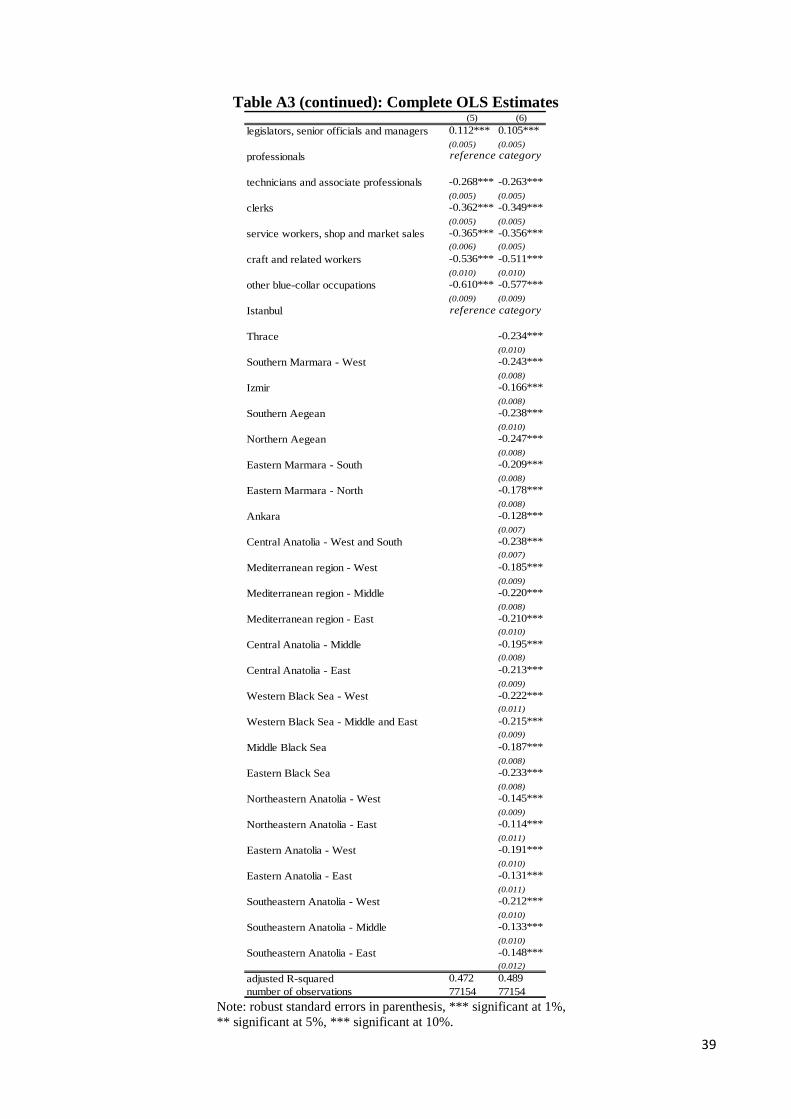
39

Table A3 (continued): Complete OLS Estimates

Note: robust standard errors in parenthesis, *** significant at 1%, ** significant at 5%, *** significant at 10%.

(5) (6)legislators, senior officials and managers 0.112*** 0.105***

(0.005) (0.005) professionals

technicians and associate professionals -0.268*** -0.263***(0.005) (0.005)

clerks -0.362*** -0.349***(0.005) (0.005)

service workers, shop and market sales -0.365*** -0.356***(0.006) (0.005)

craft and related workers -0.536*** -0.511***(0.010) (0.010)

other blue-collar occupations -0.610*** -0.577***(0.009) (0.009)

Istanbul

Thrace -0.234***(0.010)

Southern Marmara - West -0.243***(0.008)

Izmir -0.166***(0.008)

Southern Aegean -0.238***(0.010)

Northern Aegean -0.247***(0.008)

Eastern Marmara - South -0.209***(0.008)

Eastern Marmara - North -0.178***(0.008)

Ankara -0.128***(0.007)

Central Anatolia - West and South -0.238***(0.007)

Mediterranean region - West -0.185***(0.009)

Mediterranean region - Middle -0.220***(0.008)

Mediterranean region - East -0.210***(0.010)

Central Anatolia - Middle -0.195***(0.008)

Central Anatolia - East -0.213***(0.009)

Western Black Sea - West -0.222***(0.011)

Western Black Sea - Middle and East -0.215***(0.009)

Middle Black Sea -0.187***(0.008)

Eastern Black Sea -0.233***(0.008)

Northeastern Anatolia - West -0.145***(0.009)

Northeastern Anatolia - East -0.114***(0.011)

Eastern Anatolia - West -0.191***(0.010)

Eastern Anatolia - East -0.131***(0.011)

Southeastern Anatolia - West -0.212***(0.010)

Southeastern Anatolia - Middle -0.133***(0.010)

Southeastern Anatolia - East -0.148***(0.012)

adjusted R-squared 0.472 0.489 number of observations 77154 77154

reference category

reference category

40

Table A4: Selected OLS Estimates by Age Groups

Note: robust standard errors in parenthesis, *** significant at 1%, ** significant at 5%, *** significant at 10%. All regressions contain controls for wave dummies, previous potential experience (quadratic), current job tenure (quadratic), dummies for marital status, number of children, dummies for occupation and sector, quadratic firm size and dummies for nuts2 regions.

23-30 31-40 41-65education 0.020*** 0.132*** 0.012 -0.062***

(0.005) (0.011) (0.008) (0.008) arts -0.047*** -0.055** -0.035* -0.036

(0.013) (0.024) (0.019) (0.022) humanities -0.036*** 0.028* -0.067*** -0.044***

(0.007) (0.017) (0.011) (0.009) business & management

law 0.309*** 0.195*** 0.293*** 0.369***(0.013) (0.023) (0.021) (0.022)

personal services 0.002 0.030 0.006 0.002 (0.010) (0.024) (0.017) (0.015)

social sciences 0.029*** 0.076*** 0.032*** 0.001 (0.005) (0.012) (0.009) (0.008)

hard sciences 0.045*** 0.035** 0.041*** 0.052***(0.008) (0.016) (0.013) (0.013)

maths & statistics -0.009 0.001 -0.004 -0.032 (0.012) (0.025) (0.018) (0.020)

computing 0.008 0.006 0.065** 0.133***(0.014) (0.018) (0.025) (0.050)

engineering 0.067*** 0.067*** 0.071*** 0.090***(0.006) (0.010) (0.009) (0.010)

manufacturing -0.011 -0.029 -0.018 0.071***(0.012) (0.019) (0.018) (0.022)

architecture 0.044*** 0.104*** 0.057*** -0.004 (0.008) (0.016) (0.014) (0.013)

agriculture & veterinary 0.023*** 0.043*** -0.014 0.048***(0.007) (0.016) (0.012) (0.010)

health 0.410*** 0.345*** 0.431*** 0.405***(0.011) (0.025) (0.018) (0.017)

adjusted R-squared 0.489 0.508 0.425 0.366 number of observations 77154 19962 29830 27956

reference category

pooled sample

age groups

41

Table A5: Detailed Oaxaca-Blinder Decomposition

Note: z-statistics based on robust standard errors. The results are obtained from the twofold decomposition, based on the pooled estimation with the corresponding field of study dummies. All regressions contain controls for wave dummies, previous potential experience (quadratic), current job tenure (quadratic), dummies for marital status, number of children, dummies for occupation and sector, quadratic firm size and dummies for nuts2 regions.

field of studyed

ucat

ion

arts

hum

aniti

es

busi

ness

&

man

agem

ent

law

pers

onal

se

rvic

es

soci

al s

cien

ce

and

serv

ices

hard

sci

ence

s

mat

hs &

st

atis

tics

com

putin

g

engi

neer

ing

man

ufac

turin

g

arch

itect

ure

agric

ultu

re &

ve

terin

ary

heal

th

% wage difference 0.058 -0.162 0.004 -0.110 0.475 -0.172 0.053 0.058 0.040 -0.205 -0.155 -0.226 -0.008 0.030 0.595

explained 0.066 -0.081 0.071 -0.057 0.199 -0.151 0.057 0.059 0.079 -0.175 -0.197 -0.174 -0.014 0.058 0.211

wave -0.003 -0.003 -0.001 0.003 0.001 -0.003 -0.001 0.001 0.000 0.003 0.002 0.000 -0.002 -0.002 -0.002work experience 0.011 -0.031 0.058 -0.009 0.024 0.008 0.039 -0.002 -0.014 -0.121 -0.051 -0.046 -0.011 0.024 0.037family characteristics 0.007 -0.007 0.006 -0.002 0.003 -0.005 0.002 -0.002 0.005 -0.020 -0.007 -0.004 -0.004 0.003 0.007sector and firm size -0.070 -0.050 -0.088 0.038 0.081 -0.020 0.036 -0.013 -0.013 -0.030 -0.048 -0.059 -0.006 0.030 0.080occupation 0.140 -0.013 0.109 -0.097 0.079 -0.127 -0.027 0.070 0.094 -0.040 -0.099 -0.056 0.003 0.025 0.096nuts2 regions -0.018 0.022 -0.013 0.009 0.010 -0.003 0.008 0.004 0.007 0.033 0.007 -0.008 0.007 -0.021 -0.007

unexplained -0.009 -0.081 -0.066 -0.052 0.276 -0.022 -0.004 -0.001 -0.039 -0.030 0.041 -0.052 0.006 -0.028 0.384

wave 0.000 0.002 0.001 -0.001 -0.001 0.002 0.000 0.002 0.000 -0.003 0.001 0.001 0.000 0.001 0.002work experience -0.148 0.041 -0.112 0.009 -0.041 -0.040 -0.062 0.041 0.012 0.095 0.130 0.056 -0.032 -0.052 0.043family characteristics -0.005 -0.107 0.027 -0.007 0.086 -0.017 -0.002 -0.016 -0.064 -0.003 0.011 0.055 -0.006 0.074 0.023sector and firm size 0.053 -0.004 0.105 0.044 0.145 0.019 0.024 0.033 -0.095 0.034 0.076 0.043 0.011 0.028 0.008occupation -0.109 -0.047 -0.084 -0.035 0.202 -0.006 -0.024 -0.035 0.064 -0.020 0.030 0.013 0.006 -0.019 0.115nuts2 regions -0.009 0.003 -0.001 0.002 -0.001 0.012 -0.002 -0.015 -0.027 0.077 0.034 0.005 0.004 0.000 -0.022constant 0.208 0.031 -0.003 -0.064 -0.114 0.009 0.063 -0.011 0.071 -0.209 -0.241 -0.225 0.024 -0.061 0.216

42

Table A6: Detailed RIF-Regression Decomposition

quantile q1 q2 q3 q4 q5 q6 q7 q8 q9

% wage difference 0.483 0.406 0.214 0.133 0.055 0.009 -0.037 -0.130 -0.286explained 0.287 0.219 0.186 0.134 0.088 0.048 -0.004 -0.055 -0.156wave 0.001 -0.001 -0.003 -0.005 -0.005 -0.004 -0.004 -0.006 -0.005work experience 0.027 0.024 0.023 0.018 0.015 0.010 0.006 0.003 -0.010family characteristics 0.015 0.015 0.009 0.006 0.004 0.003 0.003 0.003 0.005sector and firm size 0.130 0.008 0.023 0.001 -0.029 -0.071 -0.126 -0.182 -0.307occupation 0.139 0.198 0.147 0.122 0.112 0.119 0.130 0.145 0.198nuts2 region -0.024 -0.025 -0.013 -0.008 -0.008 -0.010 -0.013 -0.018 -0.038unexplained 0.196 0.187 0.028 -0.002 -0.033 -0.039 -0.033 -0.075 -0.130wave 0.000 0.003 0.002 0.001 -0.001 0.000 0.000 -0.001 -0.001work experience 0.356 -0.429 -0.317 -0.197 -0.134 -0.104 -0.088 -0.135 -0.311family characteristics -0.051 -0.014 -0.005 0.002 0.007 0.013 0.012 0.004 0.021sector and firm size 0.563 -0.099 -0.138 -0.083 -0.051 -0.019 0.026 0.083 0.207occupation 0.335 -0.326 -0.233 -0.177 -0.155 -0.172 -0.185 -0.205 -0.257nuts2 region -0.019 -0.015 -0.009 -0.005 -0.004 -0.004 -0.005 -0.008 -0.019constant -0.989 1.066 0.728 0.458 0.305 0.247 0.206 0.188 0.230% wage difference -0.138 -0.293 -0.317 -0.229 -0.133 -0.088 -0.079 -0.082 -0.082explained -0.138 -0.237 -0.143 -0.092 -0.067 -0.051 -0.040 -0.027 0.007wave 0.000 0.001 -0.004 -0.004 -0.004 -0.003 -0.005 -0.004 -0.005work experience -0.047 -0.078 -0.049 -0.035 -0.027 -0.021 -0.015 -0.013 -0.009family characteristics -0.019 -0.018 -0.009 -0.005 -0.004 -0.003 -0.003 -0.002 -0.002sector and firm size -0.084 -0.146 -0.082 -0.048 -0.033 -0.027 -0.021 -0.017 -0.007occupation -0.026 -0.032 -0.015 -0.008 -0.005 -0.005 -0.006 -0.007 -0.010nuts2 region 0.037 0.035 0.016 0.009 0.007 0.008 0.011 0.016 0.040unexplained 0.000 -0.056 -0.174 -0.137 -0.066 -0.037 -0.040 -0.055 -0.089wave 0.007 0.000 0.000 0.000 0.003 0.001 0.003 0.002 0.004work experience -0.031 -0.104 0.324 0.307 0.108 0.020 0.008 -0.005 -0.081family characteristics -0.138 -0.181 -0.181 -0.052 -0.093 -0.045 -0.063 -0.116 -0.207sector and firm size -0.059 -0.079 -0.016 0.020 0.007 -0.021 -0.011 0.010 0.091occupation -0.171 -0.168 -0.015 0.041 0.007 -0.005 -0.025 -0.027 -0.053nuts2 region -0.022 0.023 0.082 0.073 0.027 -0.013 -0.041 -0.024 -0.055constant 0.415 0.453 -0.369 -0.527 -0.125 0.027 0.089 0.105 0.212% wage difference 0.398 0.260 0.094 0.030 -0.022 -0.062 -0.103 -0.135 -0.204explained 0.259 0.347 0.208 0.107 0.047 -0.006 -0.041 -0.077 -0.139wave 0.000 -0.001 -0.001 -0.002 -0.002 -0.002 -0.002 -0.002 -0.001work experience 0.076 0.121 0.084 0.061 0.047 0.037 0.032 0.034 0.045family characteristics 0.015 0.017 0.008 0.006 0.004 0.004 0.003 0.001 0.000sector and firm size 0.074 0.055 0.004 -0.051 -0.081 -0.121 -0.149 -0.200 -0.308occupation 0.115 0.172 0.119 0.094 0.082 0.080 0.083 0.102 0.156nuts2 region -0.023 -0.018 -0.006 -0.002 -0.002 -0.004 -0.007 -0.012 -0.032unexplained 0.139 -0.088 -0.114 -0.076 -0.069 -0.057 -0.063 -0.058 -0.065wave -0.001 0.005 0.002 0.000 0.001 0.000 0.000 0.001 0.003work experience 0.284 -0.457 -0.263 -0.166 -0.105 -0.068 -0.058 -0.068 -0.227family characteristics 0.041 0.039 0.027 0.008 0.001 0.008 0.015 0.023 0.046sector and firm size 0.457 -0.153 -0.101 -0.013 0.031 0.067 0.122 0.155 0.272occupation 0.017 -0.371 -0.197 -0.144 -0.118 -0.119 -0.122 -0.137 -0.186nuts2 region 0.013 0.008 0.007 0.004 0.000 -0.002 -0.004 -0.011 -0.017constant -0.671 0.842 0.413 0.233 0.121 0.057 -0.016 -0.020 0.044

educ

atio

nar

tshu

man

ities

43

Table A6 (continued): Detailed RIF-Regression Decomposition

quantile q1 q2 q3 q4 q5 q6 q7 q8 q9

% wage difference -0.128 -0.194 -0.155 -0.115 -0.084 -0.067 -0.036 -0.054 -0.133explained -0.108 -0.132 -0.088 -0.060 -0.041 -0.027 -0.016 -0.009 -0.034wave -0.001 0.001 0.003 0.005 0.005 0.005 0.004 0.005 0.005work experience -0.004 -0.010 -0.009 -0.008 -0.008 -0.007 -0.007 -0.010 -0.016family characteristics -0.005 -0.005 -0.003 -0.002 -0.001 -0.001 -0.001 -0.001 -0.001sector and firm size -0.007 -0.002 0.008 0.016 0.032 0.048 0.066 0.089 0.111occupation -0.106 -0.131 -0.094 -0.075 -0.072 -0.075 -0.083 -0.100 -0.150nuts2 region 0.015 0.014 0.006 0.004 0.004 0.004 0.005 0.008 0.018unexplained -0.020 -0.062 -0.067 -0.055 -0.043 -0.041 -0.020 -0.044 -0.099wave -0.002 -0.004 0.000 -0.001 0.001 -0.001 0.000 0.000 -0.006work experience -0.079 0.015 0.185 0.064 0.058 0.009 -0.023 -0.075 -0.228family characteristics 0.020 0.030 -0.015 -0.003 -0.001 -0.004 -0.010 -0.016 -0.032sector and firm size 0.023 0.072 0.131 0.047 0.029 0.006 0.013 -0.009 0.033occupation -0.144 -0.114 -0.007 -0.009 0.005 0.007 0.005 -0.015 -0.062nuts2 region -0.002 0.008 0.001 0.002 0.003 0.001 0.003 -0.004 -0.032constant 0.163 -0.069 -0.362 -0.155 -0.138 -0.057 -0.009 0.074 0.227% wage difference 0.554 0.407 0.322 0.345 0.425 0.499 0.563 0.688 0.665explained 0.281 0.420 0.250 0.176 0.148 0.147 0.155 0.168 0.160wave -0.001 0.001 0.003 0.004 0.004 0.003 0.001 0.002 0.001work experience 0.033 0.050 0.029 0.021 0.016 0.014 0.014 0.015 0.024family characteristics 0.007 0.008 0.004 0.003 0.002 0.001 0.001 0.001 0.002sector and firm size 0.139 0.211 0.117 0.073 0.061 0.067 0.074 0.073 0.009occupation 0.093 0.137 0.088 0.069 0.059 0.056 0.059 0.067 0.101nuts2 region 0.010 0.014 0.009 0.006 0.005 0.006 0.007 0.010 0.023unexplained 0.273 -0.013 0.072 0.170 0.277 0.352 0.408 0.521 0.505wave 0.006 0.005 -0.010 -0.005 -0.006 -0.007 0.010 0.010 0.000work experience -0.215 -0.523 -0.219 -0.070 0.170 0.252 0.541 0.306 -0.244family characteristics -0.048 0.156 0.168 0.091 0.094 0.075 0.173 0.131 0.055sector and firm size 0.100 -0.260 0.103 0.144 0.078 0.160 0.311 0.318 0.077occupation 0.263 0.027 0.375 0.406 0.385 0.212 0.175 0.054 -0.182nuts2 region -0.018 -0.056 -0.030 0.014 0.004 0.044 0.041 0.049 -0.023constant 0.184 0.637 -0.316 -0.411 -0.448 -0.384 -0.842 -0.348 0.822% wage difference -0.163 -0.258 -0.222 -0.159 -0.138 -0.124 -0.108 -0.115 -0.181explained -0.261 -0.293 -0.180 -0.126 -0.099 -0.085 -0.079 -0.091 -0.148wave 0.000 0.000 -0.004 -0.004 -0.004 -0.004 -0.004 -0.005 -0.004work experience 0.006 0.008 0.005 0.004 0.004 0.004 0.005 0.008 0.017family characteristics -0.010 -0.011 -0.006 -0.004 -0.003 -0.002 -0.002 -0.002 -0.004sector and firm size -0.081 -0.081 -0.042 -0.019 -0.005 0.006 0.019 0.032 0.014occupation -0.173 -0.199 -0.126 -0.099 -0.088 -0.089 -0.096 -0.123 -0.169nuts2 region -0.004 -0.009 -0.007 -0.004 -0.002 -0.001 -0.001 -0.001 -0.001unexplained 0.098 0.035 -0.042 -0.032 -0.039 -0.038 -0.030 -0.025 -0.033wave 0.003 0.003 0.000 0.002 0.002 0.001 0.003 0.002 0.002work experience -0.170 -0.053 0.205 0.040 0.049 0.078 0.015 -0.027 -0.220family characteristics -0.062 -0.061 -0.084 -0.001 0.057 0.026 0.030 0.022 0.032sector and firm size -0.049 -0.038 0.044 0.003 0.026 -0.003 0.004 -0.018 0.063occupation -0.023 -0.090 -0.024 -0.002 0.018 0.015 0.007 0.000 0.000nuts2 region 0.019 0.016 0.026 0.004 0.005 -0.003 0.001 0.019 -0.008constant 0.380 0.258 -0.209 -0.078 -0.195 -0.152 -0.090 -0.022 0.099% wage difference 0.169 0.171 0.059 0.030 0.007 0.005 0.006 0.032 0.025explained 0.101 0.141 0.062 0.032 0.023 0.025 0.037 0.046 0.048wave 0.001 0.000 -0.001 -0.002 -0.001 -0.002 0.000 -0.001 -0.001work experience 0.047 0.077 0.050 0.038 0.029 0.025 0.023 0.025 0.038family characteristics 0.004 0.004 0.002 0.001 0.001 0.001 0.001 0.000 0.000sector and firm size 0.062 0.078 0.031 0.016 0.015 0.020 0.032 0.044 0.042occupation -0.024 -0.029 -0.027 -0.026 -0.024 -0.024 -0.024 -0.030 -0.047nuts2 region 0.011 0.011 0.006 0.004 0.003 0.004 0.005 0.007 0.016unexplained 0.068 0.030 -0.002 -0.001 -0.016 -0.020 -0.030 -0.014 -0.024wave 0.003 0.006 0.001 0.000 0.000 0.000 -0.002 -0.001 0.000work experience 0.144 -0.214 -0.147 -0.070 -0.021 -0.041 -0.029 -0.043 -0.100family characteristics -0.018 -0.023 -0.007 -0.026 -0.015 -0.018 -0.013 0.000 0.029sector and firm size 0.221 -0.074 -0.069 -0.017 0.000 0.017 0.024 0.022 0.081occupation 0.070 -0.154 -0.078 -0.028 -0.020 -0.008 0.000 -0.006 -0.005nuts2 region 0.004 -0.023 -0.012 -0.003 -0.001 0.004 0.004 0.007 -0.002constant -0.356 0.510 0.310 0.143 0.040 0.025 -0.014 0.008 -0.027

busin

ess &

man

agem

ent

law

pers

onal

serv

ices

socia

l scie

nces

44

Table A6 (continued): Detailed RIF-Regression Decomposition

quantile q1 q2 q3 q4 q5 q6 q7 q8 q9

% wage difference 0.077 0.043 0.036 0.052 0.070 0.067 0.049 0.051 0.088explained 0.050 0.066 0.058 0.056 0.052 0.051 0.048 0.055 0.094wave -0.001 0.000 0.002 0.003 0.003 0.002 0.001 0.002 0.001work experience -0.009 -0.017 -0.011 -0.007 -0.005 -0.002 0.000 0.005 0.016family characteristics -0.005 -0.005 -0.003 -0.002 -0.001 -0.001 -0.001 0.000 0.000sector and firm size -0.018 -0.028 -0.003 0.003 0.002 -0.002 -0.011 -0.022 -0.032occupation 0.080 0.113 0.071 0.057 0.051 0.051 0.055 0.065 0.097nuts2 region 0.003 0.003 0.002 0.002 0.002 0.002 0.003 0.005 0.012unexplained 0.028 -0.023 -0.023 -0.004 0.018 0.016 0.002 -0.004 -0.006wave 0.003 0.004 0.004 0.004 0.000 0.004 -0.001 0.002 0.000work experience 0.019 -0.027 0.179 0.101 0.060 0.029 0.057 0.070 0.098family characteristics 0.016 0.046 0.015 0.015 0.003 0.000 -0.032 -0.054 -0.090sector and firm size -0.009 -0.016 0.022 0.003 0.008 0.004 0.012 0.062 0.169occupation 0.101 -0.066 0.015 -0.022 -0.021 -0.037 -0.053 -0.077 -0.140nuts2 region -0.015 -0.003 -0.002 -0.018 -0.014 -0.018 -0.019 -0.024 -0.016constant -0.087 0.038 -0.256 -0.086 -0.018 0.035 0.037 0.017 -0.027% wage difference 0.204 0.131 0.058 0.044 0.013 0.006 -0.011 -0.032 0.002explained 0.170 0.258 0.167 0.108 0.072 0.047 0.018 -0.013 -0.042wave 0.000 0.000 -0.001 0.000 0.000 0.000 -0.001 0.000 0.000work experience -0.022 -0.035 -0.021 -0.014 -0.010 -0.008 -0.007 -0.006 -0.005family characteristics 0.010 0.012 0.007 0.004 0.003 0.002 0.002 0.003 0.006sector and firm size 0.059 0.108 0.075 0.039 0.011 -0.014 -0.048 -0.098 -0.175occupation 0.115 0.160 0.099 0.075 0.065 0.064 0.068 0.083 0.124nuts2 region 0.009 0.012 0.007 0.004 0.003 0.004 0.003 0.004 0.009unexplained 0.034 -0.127 -0.108 -0.064 -0.059 -0.041 -0.029 -0.018 0.043wave -0.006 -0.001 -0.004 -0.003 0.000 0.001 0.001 0.000 0.001work experience 0.381 -0.038 0.012 0.012 0.020 0.032 0.035 0.025 -0.021family characteristics -0.346 -0.226 -0.088 -0.046 -0.031 0.043 0.029 0.025 0.001sector and firm size -0.054 -0.278 -0.184 -0.114 -0.092 -0.095 -0.073 -0.045 -0.155occupation 0.517 0.029 0.036 0.024 -0.003 -0.006 -0.010 -0.014 0.038nuts2 region -0.085 -0.048 -0.007 -0.002 -0.005 -0.006 -0.009 -0.026 -0.058constant -0.373 0.436 0.127 0.064 0.052 -0.010 -0.002 0.017 0.236% wage difference -0.235 -0.437 -0.484 -0.408 -0.278 -0.180 -0.091 -0.019 0.071explained -0.321 -0.512 -0.305 -0.194 -0.131 -0.096 -0.070 -0.037 0.006wave -0.001 0.001 0.003 0.005 0.006 0.004 0.004 0.005 0.003work experience -0.153 -0.243 -0.152 -0.113 -0.090 -0.077 -0.071 -0.077 -0.113family characteristics -0.047 -0.047 -0.026 -0.016 -0.011 -0.009 -0.009 -0.006 -0.009sector and firm size -0.129 -0.210 -0.115 -0.054 -0.021 0.002 0.022 0.055 0.126occupation -0.048 -0.067 -0.040 -0.032 -0.029 -0.031 -0.032 -0.036 -0.050nuts2 region 0.057 0.055 0.026 0.016 0.014 0.014 0.016 0.021 0.050unexplained 0.087 0.075 -0.180 -0.214 -0.147 -0.084 -0.021 0.018 0.065wave 0.001 -0.002 -0.007 -0.010 -0.014 -0.007 -0.006 0.001 0.010work experience -0.129 -0.107 0.088 0.193 0.215 0.149 0.109 0.065 0.258family characteristics -0.015 -0.037 -0.053 -0.074 -0.037 -0.023 -0.092 -0.028 0.161sector and firm size -0.022 -0.044 0.017 0.065 0.114 0.061 0.094 0.013 -0.041occupation -0.123 -0.144 0.019 0.085 0.107 0.074 0.042 -0.027 -0.120nuts2 region -0.015 0.045 0.078 0.152 0.139 0.116 0.101 0.064 0.100constant 0.391 0.362 -0.321 -0.625 -0.671 -0.454 -0.269 -0.070 -0.301

mat

hs &

sta

tistic

sco

mpu

ting

hard

sci

ence

s

45

Table A6 (continued): Detailed RIF-Regression Decomposition

quantile q1 q2 q3 q4 q5 q6 q7 q8 q9

% wage difference -0.221 -0.416 -0.409 -0.288 -0.156 -0.082 -0.018 0.020 0.059explained -0.388 -0.481 -0.296 -0.235 -0.174 -0.116 -0.082 -0.053 -0.032wave -0.002 0.000 0.002 0.003 0.003 0.002 0.003 0.003 0.003work experience -0.076 -0.100 -0.065 -0.055 -0.045 -0.035 -0.029 -0.029 -0.035family characteristics -0.019 -0.016 -0.009 -0.005 -0.003 -0.003 -0.003 -0.002 -0.003sector and firm size -0.192 -0.237 -0.112 -0.063 -0.032 -0.003 0.021 0.050 0.098occupation -0.117 -0.137 -0.113 -0.115 -0.097 -0.078 -0.076 -0.081 -0.108nuts2 region 0.017 0.009 0.001 0.001 0.001 0.001 0.003 0.006 0.014unexplained 0.167 0.065 -0.112 -0.052 0.018 0.034 0.064 0.072 0.090wave 0.008 0.000 -0.007 -0.006 -0.002 0.000 0.003 0.000 0.006work experience -0.189 -0.094 0.242 0.426 0.348 0.203 0.138 0.107 0.086family characteristics 0.014 0.043 0.028 0.008 0.015 0.012 0.013 0.010 0.009sector and firm size 0.061 0.056 0.106 0.150 0.102 0.038 0.033 0.024 0.050occupation -0.164 -0.032 0.114 0.154 0.122 0.082 0.059 0.039 -0.012nuts2 region 0.004 0.037 0.055 0.057 0.042 0.028 0.033 0.038 0.045constant 0.433 0.055 -0.650 -0.841 -0.610 -0.328 -0.215 -0.147 -0.094% wage difference -0.280 -0.439 -0.467 -0.350 -0.235 -0.127 -0.059 -0.062 -0.078explained -0.322 -0.503 -0.293 -0.178 -0.122 -0.091 -0.059 -0.042 -0.022wave 0.001 0.000 -0.001 -0.001 -0.002 -0.002 -0.001 -0.001 0.001work experience -0.062 -0.104 -0.067 -0.050 -0.038 -0.031 -0.025 -0.024 -0.025family characteristics -0.010 -0.010 -0.006 -0.003 -0.002 -0.002 -0.002 -0.001 -0.002sector and firm size -0.154 -0.262 -0.145 -0.073 -0.037 -0.015 0.008 0.031 0.069occupation -0.089 -0.113 -0.064 -0.044 -0.036 -0.034 -0.034 -0.040 -0.057nuts2 region -0.007 -0.014 -0.009 -0.007 -0.007 -0.007 -0.005 -0.006 -0.008unexplained 0.042 0.064 -0.174 -0.172 -0.113 -0.036 0.001 -0.020 -0.056wave 0.007 0.010 -0.001 0.000 0.004 0.002 -0.003 -0.002 -0.001work experience -0.166 -0.265 0.147 0.310 0.222 0.228 0.096 0.013 -0.053family characteristics 0.037 -0.031 -0.018 0.055 0.114 0.010 0.007 0.089 0.160sector and firm size 0.089 0.083 0.058 0.092 0.024 0.017 0.022 0.032 0.043occupation -0.102 -0.073 0.084 0.117 0.082 0.078 0.013 -0.011 -0.046nuts2 region -0.031 -0.013 0.011 0.007 0.019 0.042 0.015 0.011 -0.012constant 0.208 0.352 -0.455 -0.754 -0.578 -0.413 -0.149 -0.152 -0.147% wage difference -0.029 -0.040 -0.051 -0.008 0.006 0.035 0.049 0.037 -0.005explained -0.028 -0.100 -0.072 -0.038 -0.018 0.003 0.019 0.039 0.049wave 0.001 0.000 -0.002 -0.003 -0.003 -0.003 -0.002 -0.003 -0.002work experience -0.031 -0.051 -0.030 -0.018 -0.012 -0.007 -0.003 0.004 0.022family characteristics -0.009 -0.010 -0.006 -0.004 -0.003 -0.002 -0.002 -0.002 -0.003sector and firm size -0.030 -0.067 -0.045 -0.021 -0.005 0.011 0.026 0.041 0.036occupation 0.036 0.019 0.004 0.002 0.000 -0.002 -0.005 -0.007 -0.015nuts2 region 0.006 0.009 0.007 0.005 0.005 0.005 0.006 0.006 0.011unexplained -0.001 0.060 0.020 0.030 0.023 0.033 0.030 -0.003 -0.054wave -0.002 0.001 0.000 0.000 0.000 0.001 -0.001 0.000 0.000work experience -0.001 -0.063 0.094 0.007 0.015 0.016 -0.014 -0.020 -0.126family characteristics 0.011 0.027 0.046 0.020 -0.017 0.012 -0.014 -0.022 -0.034sector and firm size 0.015 0.041 0.067 0.072 0.039 -0.007 -0.021 -0.056 -0.029occupation 0.073 0.063 0.051 0.029 0.025 0.012 0.003 -0.026 -0.089nuts2 region -0.006 0.013 0.016 0.019 0.009 0.003 -0.001 -0.004 -0.018constant -0.091 -0.021 -0.253 -0.116 -0.047 -0.005 0.078 0.126 0.243

arch

itect

ure

engi

neer

ing

man

ufac

turi

ng

46

Table A6 (continued): Detailed RIF-Regression Decomposition

quantile q1 q2 q3 q4 q5 q6 q7 q8 q9

% wage difference 0.013 0.072 0.067 0.086 0.093 0.092 0.061 0.047 -0.050explained 0.073 0.111 0.061 0.046 0.043 0.046 0.051 0.061 0.066wave 0.000 0.000 -0.002 -0.003 -0.003 -0.002 -0.003 -0.003 -0.003work experience 0.030 0.042 0.023 0.017 0.013 0.012 0.014 0.018 0.037family characteristics 0.007 0.007 0.003 0.002 0.001 0.001 0.001 0.000 0.000sector and firm size 0.032 0.052 0.028 0.019 0.021 0.027 0.034 0.042 0.037occupation 0.040 0.047 0.027 0.021 0.017 0.016 0.015 0.018 0.029nuts2 region -0.037 -0.037 -0.017 -0.010 -0.008 -0.008 -0.010 -0.014 -0.034unexplained -0.060 -0.039 0.006 0.040 0.050 0.046 0.011 -0.014 -0.116wave 0.000 0.005 -0.001 0.001 0.000 0.000 0.002 0.002 0.000work experience 0.070 -0.066 -0.020 -0.061 -0.052 -0.072 -0.036 -0.029 -0.195family characteristics 0.078 0.214 0.119 0.065 0.064 0.054 0.056 0.038 0.058sector and firm size 0.044 0.026 0.083 0.063 0.052 0.016 -0.007 -0.013 0.019occupation 0.091 0.028 0.009 0.001 -0.005 -0.021 -0.038 -0.071 -0.161nuts2 region 0.023 0.028 0.010 -0.003 -0.005 -0.003 -0.007 -0.010 -0.022constant -0.366 -0.273 -0.195 -0.026 -0.005 0.072 0.040 0.068 0.185% wage difference 0.730 0.554 0.406 0.420 0.501 0.617 0.710 0.758 0.791explained 0.303 0.387 0.259 0.230 0.207 0.165 0.127 0.102 0.107wave 0.000 0.000 -0.002 -0.002 -0.003 -0.002 -0.003 -0.003 -0.003work experience 0.041 0.069 0.048 0.037 0.030 0.026 0.023 0.022 0.028family characteristics 0.014 0.017 0.009 0.006 0.004 0.003 0.003 0.002 0.003sector and firm size 0.121 0.135 0.092 0.100 0.103 0.072 0.043 0.017 0.003occupation 0.139 0.179 0.116 0.093 0.076 0.068 0.064 0.065 0.082nuts2 region -0.013 -0.013 -0.005 -0.003 -0.003 -0.002 -0.002 -0.003 -0.006unexplained 0.427 0.167 0.147 0.190 0.294 0.452 0.583 0.657 0.685wave 0.006 0.005 0.002 0.003 0.003 0.003 0.001 -0.005 -0.003work experience 0.045 -0.370 -0.118 0.187 0.298 0.285 0.221 0.071 -0.127family characteristics -0.015 0.018 0.015 0.048 0.042 0.035 0.026 0.023 0.063sector and firm size 0.199 -0.284 -0.210 -0.257 -0.150 -0.065 -0.037 0.043 0.091occupation 0.229 -0.149 0.063 0.201 0.186 0.073 -0.014 -0.099 -0.148nuts2 region -0.033 -0.019 -0.006 -0.009 -0.005 -0.013 -0.021 -0.028 -0.047constant -0.004 0.965 0.401 0.017 -0.080 0.134 0.406 0.653 0.856

heal

thag

ricu

lture

& v

eter

inar

y

47

Appendix B: Definition of Fields of Study 1) education: education science, training for pre-school teachers, teacher training without subject specialization, teacher training with subject specialization.

2) arts: audio-visual techniques and media production, fashion, interior and industrial design fine arts, handicrafts, music and performing arts.

3) humanities: humanities, religion and theology, history and archaeology, philosophy and ethics, languages, language acquisition, literature and linguistics.

4) business and management: business and administration (including accounting and taxation, finance, banking and insurance, management and administration, marketing and advertising, secretarial and office work, wholesale and retail sales, work skills), transport services, environment (including environmental sciences, natural environments and wildlife).

5) law: law.

6) personal services: domestic services, hair and beauty services, hotel, restaurants and catering, sports, travel, tourism and leisure.

7) social sciences and services (other): economics, political sciences, psychology, sociology and cultural studies), journalism and information (including journalism and reporting, library, information and archival studies), welfare (including care of the elderly and of disabled adults, child care and youth services, social work and counselling).

8) hard sciences: biology, biochemistry, environment (including environmental sciences, natural environments and wildlife), chemistry, earth sciences and physics.

9) mathematics and statistics: mathematics, statistics.

10) computing: information and communication technologies (ICTs, including computer use, database and network design and administration, software and applications development and analysis), computer sciences, computing, computer programming, informatics technologies (including, web design, web programming, web management, graphics, data base programming, computer technical services).

11) engineering: engineering and engineering trades (including chemical engineering and processes environmental protection technology, electricity and energy, electronics and automation, mechanics and metal trades, motor vehicles, ships and aircraft).

12) manufacturing: manufacturing and processing (including food processing, materials, textiles, mining and extraction).

13) architecture: architecture and construction (including architecture and town planning, building and civil engineering).

14) agriculture and veterinary: agriculture (crop and livestock production, horticulture), forestry, fisheries, veterinary.

48

15) Health: dental studies, medicine, nursing and midwifery, medical diagnostic and treatment technology, therapy and rehabilitation, pharmacy, traditional and complementary medicine and therapy.

Source: This list is adapted from the list provided by TURKSTAT (2016) and ISCED Fields of Education and Training, 2013 (UNESCO, 2014).

Research Institute of Applied Economics Working Paper 2013/14 , pàg. 32

Regional Quantitative Analysis Research Group Working Paper 2013/06, pag. 32