Analyzing Stock Market Movements Using Twitter Sentiment Analysis

Tushar RaoNSIT, Delhi, India

Email: rao.tushar@nsitonline.in

Saket SrivastavaIIIT-Delhi, India

Email: saket@iiitd.ac.in

Abstract—In this paper we investigate the complex relation-ship between tweet board literature (like bullishness, volume,agreement etc) with the financial market instruments (likevolatility, trading volume and stock prices). We have analyzedsentiments for more than 4 million tweets between June 2010to July 2011 for DJIA, NASDAQ-100 and 13 other big captechnological stocks. Our results show high correlation (upto0.88 for returns) between stock prices and twitter sentiments.Further, using Granger’s Causality Analysis, we have validatedthat the movement of stock prices and indices are greatlyaffected in the short term by Twitter discussions. Finally, wehave implemented Expert Model Mining System (EMMS) todemonstrate that our forecasted returns give a high value of R-square (0.952) with low Maximum Absolute Percentage Error(MaxAPE) of 1.76% for Dow Jones Industrial Average (DJIA).

Keywords-Stock market ; sentiment analysis ; Twitter ;microblogging ; social network analysis

I. INTRODUCTIONBefore the emergence of internet, information regarding

company’s stock price, direction and general sentimentstook a long time to disseminate among people. Also, thecompanies and markets took a long time (weeks or months)to calm market rumors, news or false information (memes inTwitter context). This era of web technology is marked withfast pace information dissemination as well as retrieval [1].Spreading good or bad information regarding a particularcompany, product, person etc. can be done at the click of amouse [2] or even using micro-blogging services such asTwitter. In this age of fast paced information dissemina-tion [3], short term sentiments play a very important rolein short term performance of financial market instrumentssuch as indexes, stocks and bonds.

It is well accepted that news drive macro-economic move-ment in the markets, while researches suggests that socialmedia buzz is highly influential at micro-economic level,specially in the financial markets [4], [5], [6], [7]. In thiswork we have applied simplistic message board approachby defining bullishness and agreement terminologies derivedfrom positive and negative vector ends of public sentimentw.r.t. each market security or index terms (such as returns,trading volume and volatility). This method is not onlyscalable but also gives more accurate measure of large scaleinvestor sentiment that can be potentially used for shortterm hedging strategies as discussed ahead. This gives cleardistinctive way for modeling sentiments for service basedcompanies such as Google in contrast to product basedcompanies such as Ebay, Amazon and Netflix. The aim ofthis work, is to quantitatively evaluate the effects of twittersentiment dynamics around a stocks indices/stock prices and

use it in conjunction with the standard model to improve theaccuracy of prediction.

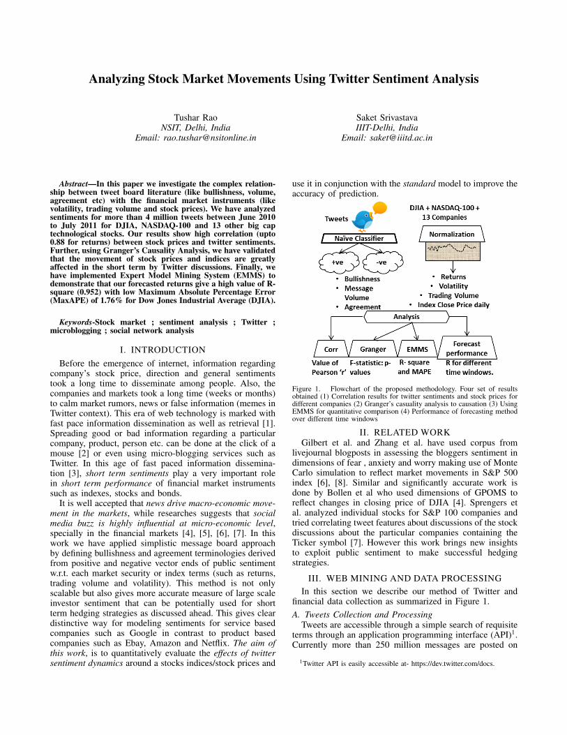
Figure 1. Flowchart of the proposed methodology. Four set of resultsobtained (1) Correlation results for twitter sentiments and stock prices fordifferent companies (2) Granger’s casuality analysis to causation (3) UsingEMMS for quantitative comparison (4) Performance of forecasting methodover different time windows

II. RELATED WORKGilbert et al. and Zhang et al. have used corpus from

livejournal blogposts in assessing the bloggers sentiment indimensions of fear , anxiety and worry making use of MonteCarlo simulation to reflect market movements in S&P 500index [6], [8]. Similar and significantly accurate work isdone by Bollen et al who used dimensions of GPOMS toreflect changes in closing price of DJIA [4]. Sprengers etal. analyzed individual stocks for S&P 100 companies andtried correlating tweet features about discussions of the stockdiscussions about the particular companies containing theTicker symbol [7]. However this work brings new insightsto exploit public sentiment to make successful hedgingstrategies.

III. WEB MINING AND DATA PROCESSINGIn this section we describe our method of Twitter and

financial data collection as summarized in Figure 1.A. Tweets Collection and Processing

Tweets are accessible through a simple search of requisiteterms through an application programming interface (API)1.Currently more than 250 million messages are posted on

1Twitter API is easily accessible at- https://dev.twitter.com/docs.

Twitter everyday (Techcrunch October 20112). This studywas conducted over a period of 14 months period betweenJune 2nd 2010 to 29th July 2011. During this period, wecollected 4,025,595 (by around 1.08M users) English lan-guage tweets Each tweet record contains (a) tweet identifier,(b) date/time of submission(in GMT), (c) language and (d)text. We have directed our focus DJIA, NASDAQ-100 and13 major companies listed in Table I. These companies aresome of the highly traded and discussed technology stockshaving very high tweet volumes.

B. Sentiment ClassificationIn order to compute sentiment for any tweet we had

to classify each incoming tweet everyday into positive ornegative using nave classifier. For each day total numberof positive tweets is aggregated as Mt

Positive while totalnumber of negative tweets as Mt

Negative. We have made useof JSON API from Twittersentiment 3, a service providedby Stanford NLP research group [9]. Online classifier hasmade use of Naive Bayesian classification method, which isone of the successful and highly researched algorithms forclassification giving superior performance to other methodsin context of tweets. Their classification training is doneover a dataset of 1,600,000 tweets and achieved an accuracyof about 82.7% [9]. In our tweet dataset roughly 61.68%of the tweets are positive, while 38.32% of the tweets arenegative for the company stocks under study. The ratio of3:2 indicates stock discussions to be much more balanced interms of bullishness than internet board messages where theratio of positive to negative ranges from 7:1 [10] to 5:1 [11];provides us with more confidence to study informationcontent of discussions about the stock prices on microblogs.

C. Tweet Feature ExtractionOne of the research questions this study explores is how

investment decisions for technological stocks are affectedby entropy of information spread about companies understudy in the virtual space. We have only aggregated the tweetparameters (extracted from tweet features) over a day. Inorder to calculate parameters weekly, bi-weekly, tri-weekly,monthly, 5 weekly and 6 weekly we have taken average ofdaily twitter feeds over the specific period of time.

Twitter literature in perspective of stock investment issummarized in Figure 1. We have carried forward work ofAntweiler et al. for defining bullishness (Bt) for each day(or time window) given as:

Bt = ln

(1 +Mt

Positive

1 +MtNegative

)(1)

Where MtPositive and Mt

Negative represent number ofpositive or negative tweets on a particular day t. Logarithmof bullishness measures the share of surplus positive signalsand also gives more weight to larger number of messages ina specific sentiment (positive or negative). Message volumefor a time interval t is simply defined as natural logarithmof total number of tweets for a specific stock/index which is

2http://techcrunch.com/2011/10/17/twitter-is-at-250-million-tweets-per-day/

3https://sites.google.com/site/twittersentimenthelp/

ln(MtPositive+Mt

Negative). The agreement among positiveand negative tweet messages is defined by:

At = 1−

√1− MPositive

t −MNegativet

MPositivet +MNegative

t

(2)

If all tweet messages about a particular company arebullish or bearish, agreement would be 1 in that case.Influence of silent tweets days in our study (trading dayswhen no tweeting happens about particular company) isless than 0.1% which is significantly less than previousresearch [11], [7]. Carried terminologies for all the tweetfeatures{Positive, Negative, Bullishness, Message Volume,Agreement} remain same for each day with the lag of oneday. For example, carried bullishness for day d is given byCarriedBullishnessd−1.

D. Financial Data CollectionWe have downloaded financial stock prices at daily inter-

vals from Yahoo Finance API4 for DJIA, NASDAQ-100 andthe companies under study given in Table I. The financial

Table ILIST OF COMPANIES

Company Name Ticker Symbol

Amazon AMZNApple AAPLAT&T TDell DELLEBay EBAYGoogle GOOGIBM IBMIntel INTCMicrosoft MSFTOracle ORCLSamsung Electronics SSNLFSAP SAPYahoo YHOO

features (parameters) under study are closing (Ct) value ofthe stock/index and the returns. Returns are calculated asthe difference of logarithm to the base e between the closingvalues of the stock price of a particular day and the previousday.

Rt = {lnClose(t) − lnClose(t−1)} × 100 (3)

Trading volume is the logarithm of number of traded shares.We estimate daily volatility based on intra-day highs andlows using Garman and Klass volatility measures [12] givenby the formula:

σ =

√1

n

∑ 1

2[ln

Ht

Lt]2 − [2 ln 2− 1][ln

Ct

Ot]2 (4)

IV. STATISTICAL ANALYSIS AND RESULTS

We begin our study by identifying the correlation betweenthe Twitter feed features and stock/index parameters whichgive the encouraging values of statistically significant rela-tionships with respect to individual stocks(indices).

4http://finance.yahoo.com/

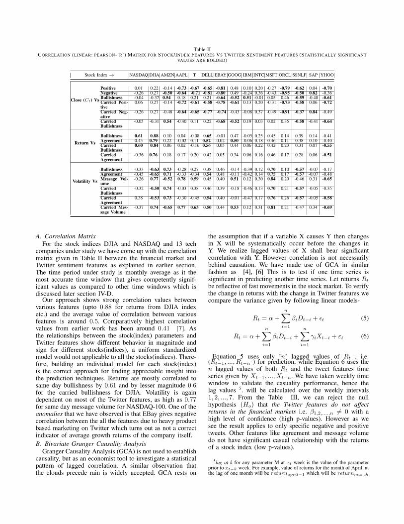
Table IICORRELATION (LINEAR: PEARSON-’R’) MATRIX FOR STOCK/INDEX FEATURES VS TWITTER SENTIMENT FEATURES (STATISTICALLY SIGNIFICANT

VALUES ARE BOLDED)

Stock Index → NASDAQ DJIA AMZN AAPL T DELL EBAY GOOG IBM INTC MSFT ORCL SSNLF SAP YHOO

Close (Ct) Vs

Positive 0.01 0.22 -0.14 -0.73 -0.67 -0.65 -0.81 0.48 0.10 0.20 -0.27 -0.79 -0.62 0.04 -0.70Negative -0.26 0.27 -0.50 -0.64 -0.71 -0.81 -0.80 0.49 -0.24 0.36 -0.43 -0.95 -0.50 0.82 -0.36Bullishness -0.04 -0.37 0.54 0.18 0.21 0.21 -0.64 -0.52 0.51 -0.01 0.05 0.46 -0.59 -0.40 -0.61Carried Posi-tive

0.06 0.27 -0.14 -0.72 -0.61 -0.58 -0.78 -0.61 0.13 0.20 -0.31 -0.73 -0.58 0.06 -0.72

Carried Neg-ative

-0.26 0.27 -0.48 -0.64 -0.65 -0.77 -0.74 -0.43 -0.08 0.37 -0.49 -0.91 -0.37 0.84 -0.49

CarriedBullishness

-0.05 -0.31 0.54 -0.40 0.11 0.22 -0.68 -0.52 0.19 0.03 0.02 0.35 -0.58 -0.41 -0.64

Return VsBullishness 0.61 0.88 0.10 0.04 -0.08 0.65 -0.01 0.47 -0.05 0.25 0.45 0.14 0.39 0.14 -0.41Agreement 0.45 0.79 0.22 -0.02 0.11 0.52 0.02 0.50 -0.06 0.18 0.46 0.11 0.38 0.10 -0.40CarriedBullishness

0.60 0.84 0.06 0.02 -0.16 0.56 0.05 0.44 0.06 0.22 0.42 0.23 0.31 0.07 -0.55

CarriedAgreement

-0.36 0.76 0.18 0.17 0.20 0.42 0.05 0.34 0.06 0.16 0.46 0.17 0.28 0.06 -0.51

Volatility Vs

Bullishness -0.33 -0.63 0.73 -0.28 0.27 0.38 0.46 -0.14 -0.39 0.12 0.70 0.10 -0.57 -0.07 -0.17Agreement -0.45 -0.65 0.71 -0.33 -0.34 0.54 0.48 -0.11 -0.42 0.14 0.75 0.17 -0.57 -0.07 -0.48Message Vol-ume

-0.26 0.77 -0.52 0.78 0.59 0.45 0.40 0.51 0.12 0.30 0.84 0.20 -0.46 0.31 -0.65

CarriedBullishness

-0.32 -0.50 0.74 -0.03 0.38 0.46 0.39 -0.18 -0.46 0.13 0.70 0.21 -0.57 -0.05 -0.35

CarriedAgreement

0.38 -0.53 0.73 -0.30 -0.45 0.54 0.40 -0.01 -0.47 0.17 0.76 0.26 -0.57 -0.05 -0.58

Carried Mes-sage Volume

-0.37 0.74 -0.65 0.77 0.63 0.50 0.44 0.53 0.12 0.31 0.81 0.21 -0.47 0.34 -0.69

A. Correlation MatrixFor the stock indices DJIA and NASDAQ and 13 tech

companies under study we have come up with the correlationmatrix given in Table II between the financial market andTwitter sentiment features as explained in earlier section.The time period under study is monthly average as it themost accurate time window that gives competently signif-icant values as compared to other time windows which isdiscussed later section IV-D.

Our approach shows strong correlation values betweenvarious features (upto 0.88 for returns from DJIA indexetc.) and the average value of correlation between variousfeatures is around 0.5. Comparatively highest correlationvalues from earlier work has been around 0.41 [7]. Asthe relationships between the stock(index) parameters andTwitter features show different behavior in magnitude andsign for different stocks(indices), a uniform standardizedmodel would not applicable to all the stocks(indices). There-fore, building an individual model for each stock(index)is the correct approach for finding appreciable insight intothe prediction techniques. Returns are mostly correlated tosame day bullishness by 0.61 and by lesser magnitude 0.6for the carried bullishness for DJIA. Volatility is againdependent on most of the Twitter features, as high as 0.77for same day message volume for NASDAQ-100. One of theanomalies that we have observed is that EBay gives negativecorrelation between the all the features due to heavy productbased marketing on Twitter which turns out as not a correctindicator of average growth returns of the company itself.B. Bivariate Granger Causality Analysis

Granger Causality Analysis (GCA) is not used to establishcausality, but as an economist tool to investigate a statisticalpattern of lagged correlation. A similar observation thatthe clouds precede rain is widely accepted. GCA rests on

the assumption that if a variable X causes Y then changesin X will be systematically occur before the changes inY. We realize lagged values of X shall bear significantcorrelation with Y. However correlation is not necessarilybehind causation. We have made use of GCA in similarfashion as [4], [6] This is to test if one time series issignificant in predicting another time series. Let returns Rt

be reflective of fast movements in the stock market. To verifythe change in returns with the change in Twitter features wecompare the variance given by following linear models-

Rt = α+

n∑i=1

βiDt−i + εt (5)

Rt = α+

n∑i=1

βiDt−i +

n∑i=1

γiXt−i + εt (6)

Equation 5 uses only ’n’ lagged values of Rt , i.e.(Rt−1, ..., Rt−n ) for prediction, while Equation 6 uses then lagged values of both Rt and the tweet features timeseries given by Xt−1, ..., Xt−n. We have taken weekly timewindow to validate the casuality performance, hence thelag values 5. will be calculated over the weekly intervals1, 2, ..., 7. From the Table III, we can reject the nullhypothesis (Ho) that the Twitter features do not affectreturns in the financial markets i.e. β1,2,....,n 6= 0 with ahigh level of confidence (high p-values). However as wesee the result applies to only specific negative and positivetweets. Other features like agreement and message volumedo not have significant casual relationship with the returnsof a stock index (low p-values).

5lag at k for any parameter M at xt week is the value of the parameterprior to xt−k week. For example, value of returns for the month of April, atthe lag of one month will be returnapril−1 which will be returnmarch

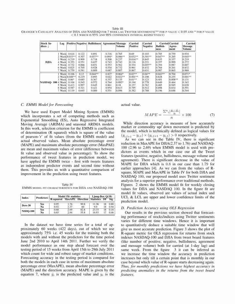
Table IIIGRANGER’S CASUALITY ANALYSIS OF DJIA AND NASDAQ FOR 7 WEEK LAG TWITTER SENTIMENTS(** FOR P-VALUE < 0.05 AND * FOR P-VALUE

< 0.1 WHICH IS 95% AND 90% CONFIDENCE INTERVAL RESPECTIVELY)

Stock In-dices ↓

Lag Positive Negative Bullishness Agreement MessageVolume

CarriedPositive

CarriedNegative

CarriedBullish-ness

CarriedAgree-ment

CarriedMessageVolume

DJIA

1 Week 0.614 0.122 0.891 0.316 0.765 0.69 0.103 0.785 0.759 0.9342 Week 0.033** 0.307 0.037** 0.094* 0.086** 0.032** 0.301** 0.047** 0.265 0.045**3 Week 0.219 0.909 0.718 0.508 0.237 0.016** 0.845 0.635 0.357 0.2194 Week 0.353 0.551 0.657 0.743 0.743 0.116 0.221 0.357 0.999 0.2725 Week 0.732 0.066 0.651 0.553 0.562 0.334 0.045** 0.394 0.987 0.6076 Week 0.825 0.705 0.928 0.554 0.732 0.961 0.432 0.764 0.261 0.8327 Week 0.759 0.581 0.809 0.687 0.807 0.867 0.631 0.987 0.865 0.969

NASDAQ- 100

1 Week 0.106 0.12 0.044** 0.827 0.064* 0.02** 0.04** 0.043** 0.704 0.071*2 Week 0.048** 0.219 0.893 0.642 0.022** 0.001** 0.108 0.828 0.255 0.001**3 Week 0.06* 0.685 0.367 0.357 0.135 0.01** 0.123 0.401 0.008** 0.1314 Week 0.104 0.545 0.572 0.764 0.092* 0.194 0.778 0.649 0.464 0.3435 Week 0.413 0.997 0.645 0.861 0.18 0.157 0.762 0.485 0.945 0.0286 Week 0.587 0.321 0.421 0.954 0.613 0.795 0.512 0.898 0.834 0.5917 Week 0.119 0.645 0.089 0.551 0.096 0.382 0.788 0.196 0.648 0.544

C. EMMS Model for Forecasting

We have used Expert Model Mining System (EMMS)which incorporates a set of competing methods such asExponential Smoothing (ES), Auto Regressive IntegratedMoving Average (ARIMA) and seasonal ARIMA models.In this work, selection criterion for the EMMS is coefficientof determination (R squared) which is square of the valueof pearson-’r’ of fit values (from the EMMS model) andactual observed values. Mean absolute percentage error(MAPE) and maximum absolute percentage error (MaxPAE)are mean and maximum values of error (difference betweenfit value and observed value in percentage). To show theperformance of tweet features in prediction model, wehave applied the EMMS twice - first with tweets featuresas independent predictor events and second time withoutthem. This provides us with a quantitative comparison ofimprovement in the prediction using tweet features.

Table IVEMMS MODEL FIT CHARACTERISTICS FOR DJIA AND NASDAQ-100

Index Predictors Model Fit statistics Ljung-Box Q(18)R-squared MaxAPE Direction Statistics DF Sig.

Dow-30 Yes 0.95 1.76 90.8 11.36 18 0.88No 0.92 2.37 60 9.9 18 0.94

NSDQ-100 Yes 0.68 2.69 82.8 23.33 18 0.18No 0.65 2.94 55.8 16.93 17 0.46

In the dataset we have time series for a total of ap-proximately 60 weeks (422 days), out of which we useapproximately 75% i.e. 45 weeks for the training both themodels with and without the predictors for the time periodJune 2nd 2010 to April 14th 2011. Further we verify themodel performance as one step ahead forecast over thetesting period of 15 weeks from April 15th to 29th July 2011which count for wide and robust range of market conditions.Forecasting accuracy in the testing period is compared forboth the models in each case in terms of maximum absolutepercentage error (MaxAPE), mean absolute percentage error(MAPE) and the direction accuracy. MAPE is given by theequation 7, where yi is the predicted value and yi is the

actual value.

MAPE =Σn

i|yi−yi

yi|

n× 100 (7)

While direction accuracy is measure of how accuratelymarket or commodity up/ down movement is predicted bythe model, which is technically defined as logical values for(yi,t+1 − yi,t)× (yi,t+1 − yi,t) > 0 respectively.

As we can see in the Table IV, there is significantreduction in MaxAPE for DJIA(2.37 to 1.76) and NASDAQ-100 (2.96 to 2.69) when EMMS model is used with pre-dictors as events which in our case our all the Tweetfeatures (positive, negative, bullishness, message volume andagreement). There is significant decrease in the value ofMAPE for DJIA which is 0.8 in our case than 1.79 forearlier approaches [4]. As we can from the values of R-square, MAPE and MaxAPE in Table IV for both DJIA andNASDAQ 100, our proposed model uses Twitter sentimentanalysis for a superior performance over traditional methods.Figures 2 shows the EMMS model fit for weekly closingvalues for DJIA and NASDAQ 100. In the figure fit aremodel fit values, observed are values of actual index andUCL & LCL are upper and lower confidence limits of theprediction model.

D. Prediction Accuracy using OLS RegressionOur results in the previous section showed that forecast-

ing performance of stocks/indices using Twitter sentimentsvaries for different time windows. Hence it is importantto quantitatively deduce a suitable time window that willgive us most accurate prediction. Figure 3 shows the plot ofR-square metric for OLS regression for returns from stockindexes NASDAQ-100 and DJIA from tweet board features(like number of positive, negative, bullishness, agreementand message volume) both for carried (at 1-day lag) andsame week. From the figure 3 it can be inferred aswe increase the time window the accuracy in predictionincreases but only till a certain point that is monthly in ourcase beyond which value of R-square starts decreasing again.Thus, for monthly predictions we have highest accuracy inpredicting anomalies in the returns from the tweet boardfeatures.

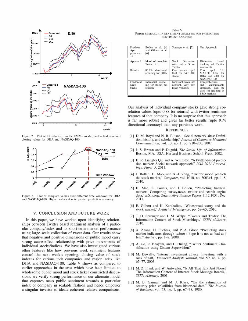
Figure 2. Plot of Fit values (from the EMMS model) and actual observedclosing values for DJIA and NASDAQ-100

Figure 3. Plot of R-square values over different time windows for DJIAand NASDAQ-100. Higher values denote greater prediction accuracy.

V. CONCLUSION AND FUTURE WORK

In this paper, we have worked upon identifying relation-ships between Twitter based sentiment analysis of a partic-ular company/index and its short-term market performanceusing large scale collection of tweet data. Our results showthat negative and positive dimensions of public mood carrystrong cause-effect relationship with price movements ofindividual stocks/indices. We have also investigated variousother features like how previous week sentiment featurescontrol the next week’s opening, closing value of stockindexes for various tech companies and major index likeDJIA and NASDAQ-100. Table V shows as compared toearlier approaches in the area which have been limited towholesome public mood and stock ticker constricted discus-sions, we verify strong performance of our alternate modelthat captures mass public sentiment towards a particularindex or company in scalable fashion and hence empowera singular investor to ideate coherent relative comparisons.

Table VPRIOR RESEARCH IN SENTIMENT ANALYSIS FOR PREDICTING

SENTIMENT ANALYSIS

PreviousAp-proaches→

Bollen et al. [4]and Gilbert et al.[6]

Sprenger et al. [7] Our Approach

Approach Mood of completeTwitter feed

Stock Discussionwith ticker $ onTwitter

Discussion basedtracking of Twittersentiments

Results 86.7% directionalaccuracy for DJIA

Corr values uptil0.41 for S&P 100stocks

Corr uptil 0.9,MAXPE 1.76 forDJIA and 2.69 forNASDAQ-100

Feedback/Draw-backs

Individual model-ing for stocks notfeasible

News not taken intoaccount, very lesstweet volumes

Comprehensiveand customizableapproach. Can beused for hedging inF&O markets

Our analysis of individual company stocks gave strong cor-relation values (upto 0.88 for returns) with twitter sentimentfeatures of that company. It is no surprise that this approachis far more robust and gives far better results (upto 91%directional accuracy) than any previous work.

REFERENCES

[1] D. M. Boyd and N. B. Ellison, “Social network sites: Defini-tion, history, and scholarship,” Journal of Computer-MediatedCommunication, vol. 13, no. 1, pp. 210–230, 2007.

[2] J. S. Brown and P. Duguid, The Social Life of Information.Boston, MA, USA: Harvard Business School Press, 2002.

[3] H. R. Liangfei Qiu and A. Whinston, “A twitter-based predic-tion market: Social network approach,” ICIS 2011 Proceed-ings. Paper 5, 2011.

[4] J. Bollen, H. Mao, and X.-J. Zeng, “Twitter mood predictsthe stock market,” Computer, vol. 1010, no. 3003v1, pp. 1–8,2010.

[5] H. Mao, S. Counts, and J. Bollen, “Predicting financialmarkets: Comparing survey,news, twitter and search enginedata,” arXiv.org, Quantitative Finance Papers 1112.1051, Dec.2011.

[6] E. Gilbert and K. Karahalios, “Widespread worry and thestock market,” Artificial Intelligence, pp. 58–65, 2010.

[7] T. O. Sprenger and I. M. Welpe, “Tweets and Trades: TheInformation Content of Stock Microblogs,” SSRN eLibrary,2010.

[8] X. Zhang, H. Fuehres, and P. A. Gloor, “Predicting stockmarket indicators through twitter i hope it is not as bad as ifear,” Anxiety, pp. 1–8, 2009.

[9] A. Go, R. Bhayani, and L. Huang, “Twitter Sentiment Clas-sification using Distant Supervision.”

[10] M. Dewally, “Internet investment advice: Investing with arock of salt,” Financial Analysts Journal, vol. 59, no. 4, pp.65–77, 2003.

[11] M. Z. Frank and W. Antweiler, “Is All That Talk Just Noise?The Information Content of Internet Stock Message Boards,”SSRN eLibrary, 2001.

[12] M. B. Garman and M. J. Klass, “On the estimation ofsecurity price volatilities from historical data,” The Journalof Business, vol. 53, no. 1, pp. 67–78, 1980.