Transportation Research Record 1058

2. J.C. Vance. Liability of the State for Highway Traffic Noise. In Selected Studies in Highway Law, Vol. 2. NCHRP, Transportation Research Board, Washington, D.C., 1982.

3. C.L. Northcutt and Theo D. Northcutt v. State Road Department of Florida. Vol. 209 Southern Reporter (second series), 1968, pp. 710-714.

4. Florida Eminent Domain Practice and Procedure, 3rd ed. Florida Bar, Tallahassee, 1977.

5. Division of Administration, State of Florida De­partment of Transportation v. West Palm Beach

23

Garden Club, et al., Vol. 352 Southern Reporter (second series), 1978, pp. 1177-1182.

6. J.W. Scruggs, Jr. Recommendation of Settlement. Florida Department of Transportation, Office of Eminent Domain, Tallahassee, Jan. 17, 1985.

Publication of this paper sponsored by Committee on Transportation-Related Noise and Vibration.

Analyzing Construction Noise by a Level/Duration

Weighted Population Technique

WILLIA.l\f BOWLBY, ROSWELL A. HARRIS, and LOUIS F. COHN

ABSTRACT

A technique is described for comparing the potential noise impacts of construc­tion hauling for a number of project alternatives. The technique is used on a modification of the level weighted population method to account for the dura­tion of the hauling activity on the various haul route links; the resultant descriptor is termed Level/Duration Weighted Population (LDWP). A complex microcomputer spreadsheet was developed to facilitate data entry and calcula­tion of LDWP for a base case and each study scenario, as well as a relative change in impact (RCI) over the base case for the scenarios.

River flood control construction projects funded by the U.S. Army Corps of Engineers require environ­mental assessments. Project alternatives typically include the construction of tall levees or flood walls or the cutting of channels to divert the river flow from floodplain. Such projects can take as long as 6 to 7 years to construct; hence, a serious po­tential impact of the project can be construction noise--in particular, the extensive material-hauling operations.

To assess and compare the construction haul-noise impacts of a set of different alternatives for a flood control project in Harlan, Kentucky, a tech­nique was developed that considered existing commu­nity noise levels, future haul-noise levels, dura­tion of haul activities, and population densities. In this paper that technique is described; it was implemented with a sophisticated microcomputer spreadsheet program.

w. Bowlby, Vanderbilt University, Box 96-B, Nash­ville, Tenn. 37235. R.A. Harris and L.F. Cohn, Speed Scientific School, University of Louisville, Ky. 40292.

PROBLEM DEFINITION

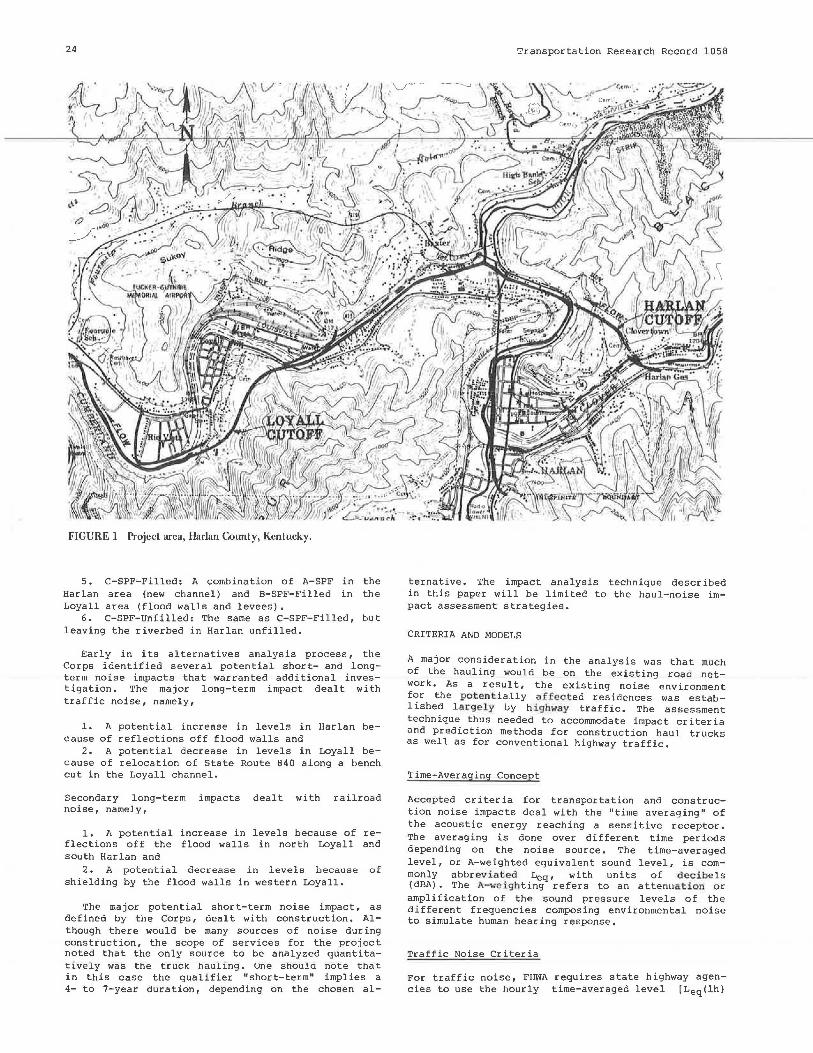
Harlan, Kentucky, and its neighboring communities of Loyall, Rio Vista, and Baxter ar.e located along the Cumberland River and two of its forks in Southeast Kentucky (1). The study area, sh~wn in Figure 1, is characteri;ed by steep-sided valleys with most of the commercial and residential development concen­trated in narrow floodplains. Major floods occur mostly in the winter or spring; the flood of record, in April 1977, crested at over 30 ft above gauge zero. To minimize potential future damage, the Corps is evaluating a series of alternatives for flood control (.!_). These alternatives include the follow­ing:

1. A-77: Building levees and flood walls in the Harlan and Loyall areas for the 1977 flood levels.

2. A-SPF: Same as A-77, but for the Standard Projected Flood level.

3, B-SPF-Filled: Cutting new channels through the 200- to 300-ft high hills behind Harlan and Loyall, building diversion dikes along the river at the ends of these channels, and filling in the ex­isting riverbeds between the diversion dikes.

4, B-SPF-Unfilled: Same as B-SPF-Filled, but leaving the riverbeds unfilled in the diversion areas.

24

FIGURE I Project area, Harlan County, Kentucky.

5. C-SPF-Filled: A combination of A-SPF in the Harlan area (new channel) and B-SPF-Filled in the Loyall area (flood walls and levees).

6. C-SPF-Unfilled: The same as C-SPF-Filled, but leaving the riverbed in Harlan unfilled.

Early in its alternatives analysis process, the Corps identified several potential short- and long­term noise impacts that warranted additional inves­tigation. The major long-term impact dealt with traffic noise, namely,

1. A potential increase in levels in Harlan be­cause of reflections off flood walls and

2. A potential decrease in levels in Loyall be­cause of relocation of State Route 840 along a bench cut in the Loyall channel.

Secondary long-term impacts dealt with railroad noise, namely,

1. A potential increase in levels because of re­flections off the flood walls in north Loyall and south Harlan and

;;. • A potential decrease in levels because of shielding by the flood walls in western Loyall.

The major potential short-term noise impact, as defined by the Corps, dealt with construction. Al­though there would be many sources of noise during construction, the scope of services for the project noted that the only source to be analyzed quanti ta­tively was the trucK hauling. une should note that in this case the qualifier "short-term" implies a 4- to 7-year duration, depending on the chosen al-

Transportation Research Record 1058

ternative. The impact analysis technique described in this paper will be limited to the haul-noise im­pact assessment strategies.

CRITERIA AND MODELS

A major consideration in the analysis was that much of the hauling would be on the existing road net­work. As a result, the existing noise environment for the potentially affected residences was estab-1 ished largely by highway traffic. The assessment technique thus needed to accommodate impact criteria and prediction methods for construction haul trucks as well as for conventional highway traffic.

Time-Averaging Concept

Accepted er i ter ia for transportation and construc­tion noise impacts deal with the "time averaging" of the acoustic energy reaching a sensitive receptor. The averaging is done over different time periods depending on the noise source. The time-averaged level, or A-weighted equivalent sound level, is com­monly abbreviated Leqr with units of decibels (dBA). The A-weighting refers to an attenuation or amplification of the sound pressure levels of the different frequencies composing environmental noise to simulate human hearing response.

Traffic Noise Criteria

For traffic noise, FHWA requires state highway agen­cies to use the hourly time-averaged level [Leq(lh)

Bowlby et al.

or Leq(h)] or the hourly 10th-percentile exceedance level [L10 (h) l (~). Traffic noise predictions are done for the "worst" noise hour, which typically oc­curs during the daytime, inclusive of the morning and evening rush periods,

The FHWA noise standards (2) indicate that noise mitigation must be considered- when (a) the future "design-year" project levels "substantially exceed" existing levels and (b) the future levels "approach or exceed" stated noise abatement criteria. For res­idential land use, the criterion is an Leq(lh) of 67 dBA, Note that these criteria define when mitiga­tion must be considered, not when an impact occurs. Although not stated in the noise standards, subse­quent FHWA policy guidance suggests that impacts oc­cur when the Leq(lh) exceeds 55 dBA (~). The stan­dards also do not define the phrase "substantially exceed," although many agencies have settled on an increase of 10 to 15 dBA as an indication of impacts worthy of mitigation study.

Construction Noise Criteria

For construction noise, the U.S. Army Construction Engineering Research Laboratory (CERL) supports use of a measure called the representative level (LA) (~) • LA is defined by a Society of Automotive Engi­neers (SAE) measurement procedure, which was devel­oped before the common availability of integrating sound-level meters (2), as follows:

n

LA= l (LA)i/n I=l

(1)

where (LA)i are those sound-level samples that fall within a range from the maximum sampled level to 6 dB less than the maximum sampled level [e.g., if the maximum sampled level was 70 dB, all sound-level samples from 64 to 70 dB would be (LA) i values] and n is the number of (LA)i values used for computing the arithmetic average.

LA is related to the time-averaged level (Leql by the fraction of samples within 6 dB of the highest:

Leq LA - t. (2)

where

t. 0 dB for 0.8 < (n/60) .s. 1.0, 1 dB for 0.7 < (n/60) .s. 0.8, 2 dB for 0.6 < (n/60) .s. 0. 7,

.. 3 dB for 0.5 < (n/60) .s. 0.6, = 4 dB for 0.4 < (n/60) < 0 .5,

5 dB for 0.3 < (n/60) 3: 0.4, "" 7 dB for 0.2 < (n/60) < 0.3, and

10 dB for 0 < (n/60) < 0.2.

The CERL specifications do not specify a particu­lar period over which levels should be averaged, al­though use of the SAE procedure will typically re­quire at least 30 min of data collection. CERL simply specifies daytime and nighttime periods.

In addition, the CERL impact criteria specifica­tions address noise generated within the construc­tion boundary; they do not address trucks hauling beyond the site (~_) • Nor does the FHWA have con­struction noise impact criteria; as guidance, it suggests that users could develop their own criteria by considering absolute levels as well as relative differences in levels (§) •

The FHWA noise standards address construction noise but do not require prediction of construction noise levels for federal-aid highway projects (~).

25

However, FHWA models are available that predict 1-hr or 8-hr time-averaged levels [Leq(lh) or LeqC8h)] <lr.~) • One component noise source in the FHWA con­struction noise model is the haul truck. The model requires specification of an hourly flow rate (trucks per hour), thus assuming a constant flow throughout the day. As a result, the predicted hourly Leq will be equal to the 8-hr average. Because haul-truck noise generation is so similar to normal highway truck noise generation and because the haul trucks will often travel the same paths as does the normal traffic, the most appropriate measure for studying haul-truck noise for this project was the hourly Leq or Leq(lh).

Reiative Change in Impact

Because this study needed to gauge the impact of the introduction of the construction haul traffic to a static situation, it was appropriate to use some method of comparing "build" and "no-build" levels. Such a method was described by Kugler et al. in 1976 (§). The method is based on the concept of the level-weighted population (LWP), also referred to as "fractional impact." The method uses the "day-night" time-averaged level, or Lan• which is a 24-hr average of acoustic energy where 10 dB is added to all val­ues between 10:00 p.m. and 7:00 a.m. as a penalty for nighttime sensitivity.

A scale is established where an Lan of 55 dB is assumed to "highly annoy" zero percent of the popu­lation, whereas an Lan of 75 dB is assumed to highly annoy 100 percent of the population. The number of people exposed to different Lan values for each case is then weighted according to the I.an values. An "equivalent highly annoyed" population (or level-weighted population) is then computed for the base case and the alternative being studied. Mathematically,

n LWP (3)

i=l

where Pi is the number of people exposed to day­n ight level <Lanli and n is the number of Lan values or ranges used in the calculations typically; the calculation is performed by grouping subjects in 5-dB Lan bands.

A relative change in impact puted by subtracting the LWP (LWPbasel from the LWP for

(RCI) is then com­for the base case

the alternative (LWPa1tl, dividing by the base-case LWP, and mul­tiplying by 100:

RCI = [(LWPal t - LWPbasel /LWPbase] x 100 (4)

The LWP values for each case are also good indi­cators of the absolute impact as compared with an Lan of 55 dB. The RCI method has been used for nontraffic noise sources as well, as illustrated in the U.S. Environmental Protection Agency background document on rail carrier noise standards (1).

For the flood control study, it appeared that a slightly modified version of the RCI method was the most appropriate to compare the various construction haul scenarios for each project alternative. Instead of using a 24-hr Lan• which is appropriate rail­road noise, the hourly Leq was used. Kugler et al., as well as the EPA, suggested that an Lan of 55 dB was an indicator of zero percent highly annoyed. As noted ear lier, FHWA considers a traffic noise Leq (lh) of 55 dB to also represent no impact. Given the similarity of haul-truck noise to traffic noise, the construction noise LWP values could also be computed

26

by using a 55-dB Leq ( lh) as the base line value. The LWP for the various construction ha ul scenarios could then be compared with a base-case LWP, which would be caused by traff i c nois e with no project haul trucks. Thus, the relative impacts of each haul

-----""~ y compu l.On o e I .

Traffic Noise Model

Once this means of quantifying and comparing impacts had been selected, the next step was to choose models to prP.cHct future noise leve1·s for traffic and construction haul trucks.

The accepted model for traffic noise is the FHWA Highway Traffic Noise Prediction Model (10), which consists of the basic acoustics equations for sound emission a nd p r opagat i on and at t enuation by bar­riers. Several methods are ava ilable for using the model, including charts, nomographs, and various levels of computer programs. The nomograph method was the most appropriate for predicting base-case traffic noise levels given the general nature of the site modeling.

Several methods are available to predict haul­truck noise, including the FHWA HICNOM computer pro­gram (!!l and the FHWA Highway Traffic Noise Predic­tion Model <lQ). The methods are similar in concept for the truck noise source, differing in the values for the basic emission-level equation. On the basis of observations by the study team during field sound-level measurements, the trucks currently in use in the project area for hauling coal have emis­sion levels similar to the typical heavy truck modeled in the FHWA traffic noise model. These coal haul trucks, including muffler systems, are rela­tively new and generally well maintained. It was anticipated that many of these same, or similar, trucks would be employed for hauling during the flood control project construction. Therefore, it was appropriate to model them by using the heavy­truck vehicle type in the FHWA traffic noise model and use that model to predict hourly haul-truck Leq-values.

STUDY METHOD

The study method cons isted of a series of steps. First, the LWP technique needed to be modified to incorporate the duration of cons t r uction hauling in a particular area. This modific ation was a key fac­tor in the analysis technique. Next, a haul network and haul scenarios were developed for each project alternative. Then, base-case impacts were determined as a basis for comparison with hauling impacts. Fi­nally, the hauling impacts were determined and used to compute changes in impact relative to the base case. These steps are discussed in detail in the following paragraphs.

Consideration of Haul Duration

As noted earlier, the RC! technique is based on the fractional impact or LWP concept, which, in its sim­plest form, states that the impact on a few people exposed to high noise levels is equivalent to the impact on a larger number of people exposed to lower noise levels. In this technique, a person exposed to a level of 55 dB or less is assumed to receive zero impact, whereas a person exposed to a level of 75 dB is assumed to receive 100 percent impact. A linear change in impaci.. i~ i:.ht=n applied for those exposed to levels between 55 and 75 dB; for example, a per­son would be considered 25 percent impacted a t a

Transportation Research Record 1058

level of 60 dB, 50 percent impacted at a level of 65 dB, and 75 percent impacted at a level of 70 dB.

The technique then involves the weighting of the population according to the noise -level exposures to de t ermine a n e u i valent · cent impacted. This normalization procedure thus gives a meaningful method to compare the relative differences between scenarios and hence alternatives.

Construction noise analysis has an additional factor that needed to be considered. Traffic noise, which forms the base case or "do-nothing" alterna­tive, is typically considered a permanent type of noicc. However, construction is a temporary noise of finite duration. The analysis technique thus needed to account for the duration of the haul activities. For example, it is obvious that a person exposed to noise from 100 haul trucks per hour for 2 years would be more seriously impacted than a person ex­posed to the same number of trucks for a 1-year pe­riod. The question is how to quantitatively compare the impact of the two situations.

Guidance may be found in the CERL report on con­struction noise specifications (_!) , in which a log­arithmic relationship is used when durations are considered in its "maximum permissible" noise-level specification, normalized to a 32-day period. Spe­cifically, each halving of the duration of the ac­tivity would raise the perm i ss i ble noise level by 3 dB. Mathematically,

6duration = 10 log (duration/32) (5)

Choice of the 32-day period by CERL was arbitrary, probably a compromise on a 1-month' s duration and a factor of 2 for ease of calculation. Thus, just as the dwelling units are normalized to an equivalent population that was 100 percent impacted, the haul operations of varying durations may be normalized to some base-case value. In this manner, one may rede­fine the LWP as a level/duration weighted population, or LDWP.

During project discussions, it was determined that the longest construction period for any of the alternatives would be approximately 7 years. It was decided therefore to normalize the levels to this period. Based on an assumption of 45 work weeks per year, a 7-year period equaled 315 weeks. Thus, the construction haul noise levels were adjusted for the LDWP calculation by

6duration = 10 log (duration/315) (6)

Repre sentative Distance Bands

In performing the fractional impact analysis, one could predict a precise noise level at every house along a project haul-road link. However, given the nature of the analysis, such precision would be un­warranted and probably deceiving. A much more effi­cient method, with little loss in overall accuracy, would be to group the dwelling units on the basis of their distances from the haul link.

To accomplish this grouping, representative dis­tance bands needed to be defined. Typical distances for traffic noise predictions are 25, 50, 100, 200, and 400 ft. Based on sound-level propagation calcu­lations, five distance bands were defined: 10 . to 35 ft, 35 to 70 ft, 70 to 165 ft, 165 to 280 ft, and 280 to 560 ft. The band outer limits are such that for soft-site propagation (grassy ground cover) the level at a house located anywhere within a given band would be within 2.2 dB of the level at the cor­responding representative distance.

Noise levels could then be computed at the five representative distances, and those levels applied

Bowlby et al.

to all the houses within the corresponding distance bands. Thus, knowing the noise levels, adjusted for duration of activity, and the number of people ex­posed to those duration-corrected levels, one could compute an LDWP for a hauling scenario for a project alternative.

Development of a Hauling 'Network and Hauling Scenarios

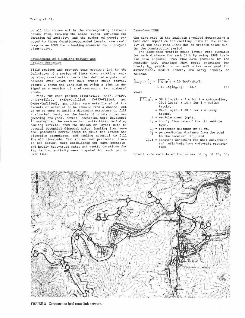
Field reviews and project team meetings led to the definition of a series of links along existing roads or along construction roads that defined a potential network over which the haul trucks could travel. Figure 2 shows the link map on which a link is de­fined as a section of road connecting two numbered roads.

Then, for each project alternative (A-77, A-SPF, B-SPF-Filled, B-SPF-Unfilled, C-SPF-Filled, and C-SPF-Unfilled), quantities were established of the amounts of material to be removed from a channel cut or to be used to build a diversion structure or fill a riverbed. Next, on the basis of construction se­quencing analyses, several scenarios were developed to accomplish the various haul activities, including hauling material from the Harlan or Loyall cuts to several potential disposal sites, hauling from sev­eral potential borrow areas to build the levees and diversion structures, and hauling material to fill the old riverbeds. Haul routes over particular links in the network were established for each scenario, and hourly haul-truck rates and weekly durations for the hauling activity were computed for each perti­nent link.

FIGURE 2 Construction haul route link network.

27

Base-Case LDWP

The next step in the analysis involved determining a base-case impact on the dwelling units in the vicin­ity of the haul-road links due to traffic noise dur­ing the construction period.

The base-case traffic noise levels were computed for each distance for each link by using 1989 traf­fic data adjusted from 1982 data provided by the Kentucky DOT. Standard FHWA model equations for hourly Leq prediction on soft sites were used for automobiles, medium trucks, and heavy trucks, as follows:

where

[(L0 ) Eh + 10 log (Ni D0 /S)

+. 15 log(Do/Dj) - 33.4 (7)

38.1 log(S) - 2.4 for i = automobiles, 33.9 log(S) + 16.4 for i medium trucks, 24.6 log(S) + 38.5 for i heavy trucks,

S vehicle speed (mph), Ni hourly flow rate of the ith vehicle

type,

33.4

reference distance of 50 ft, perpendicular distance from the road to the receiver (ft), and constant adjusting for unit conversion and infinitely long soft-site propaga­tion.

Levels were calculated for values of Dj of 25, 50,

28

100, 200, and 400 ft. Then, the [LeqCh) il were combined for the total hourly average level on the link at each distance [l.eq(h)T]:

values sound

Transportation Research Record 1058

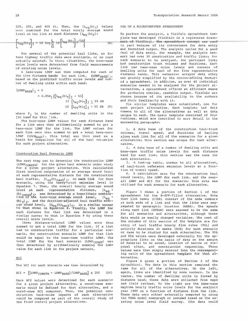
USE OF A MICROCOMPUTER SPREADSHEET

To perform the analysis, a VisiCalc spreadsheet tem-plate was developed (VisiCalc is a registered trade­

rLeqiiTty~:04.~i ~,_,(...._h,_,)_..i].!4-jL/_.._l,,_0 1-l------(•~8~)---llll;A<C10i-!CHk1-<0)Jf._,1>l-'./ ii,s-s~~ds~net':•"P""l-w-a-s~o~s~e·A--------l JJ - .-,, Ii -- L - J { in part because of its convenience for data entry

For several of the potential haul links, no fu­ture highway traffic data were available, or no road actually existed. In these situations, the base-case noise levels were determined from field measurements of existing noise levels.

A base-case LDWP was then computed for each of the five distance bands for each link, (LDWPuAsEljr based on the predicted traffic noise levels and num­ber of dwelling units within each band:

(LDWPBASE) j 0

o.05Pjj[LeqChlT]j - 55f

if [LeqChlT]j < 55 dB

if [Leq(h) T] j > 55 dB (9)

where P · is the number of dwelling units in the j th bancf for this link.

The base-case LDWP values for each distance band for a link were then arithmetically summed to get a base-case LDWP for the link. The LDWP values for each link were then summed to get a total base-case LDWP (LDPWaAsE>. This total was then used as a basis for comparison for all of the haul scb1ar ios for each project alternative.

Construction Haul Scenario LDWP

The next step was to determine the construction LDWP (LDWPcoNSTR) for the given haul scenario under study for a given project alternative. This calculation first involved computation of an average sound level at each representative distance for the construction haul traffic, [Leq(hlhaulljr on each link for that scenario, using the heavy-truck emission level in Equation 7. Then, the overall hourly average sound level at each representative distance , [Leq • (~lcon$ tl~, was determined by a logarithmic combina­tion Of t e base-case average sound level, [Leq • (h) T]j , and the duration-adjusted haul traffic aver­age sound level, C!.eg(hlha~ill j • ~n a s i milar manner to that shown in Equation 8. Finally, the LDWP for each distance for that link was determined in a similar manner to that in Equation 9 by using these overall noise levels.

'l'hese distance-related LDWP values were then summed to get a total LDWP for the link. If a link had no construction traffic for a particular sce­nario, the construction scenario LDWP for that link would be equal to the base-case traffic LDWP. The total LDWP for the haul scenario (LDWPcoNsT) was then determined by arithmetically summing the LDWP value for each link in the project network.

The RCI for each scei-1ar io was then determined by

RC! = [(LDWPcoNSTR - LDWPBASE)/LDWPBASE] x 100 (10)

Once RC! values were determined for each scenario for a given project alternative, a worst-case sce­nario could be defined for that alternative, and a worst-case RCI computed. Thus, the potential con­struction haul-noise impacts of each alternative could be compared as part of the overall study of the flood control project alternatives.

and formatted output. The analysis called for a good deal of data entry. For example, the analysis net­work had over 30 construction and traffic links; for each scenario to be analyzed, the pertinent links had construction truck volumes and durations. Each link had base-case noise levels and numbers of dwelling units for each of the five representative distance bands. This extensive arrayed data entry was greatly simplified by the screen-editing feature of a spreadsheet. In addition, as over 40 individual scenarios needed to be analyzed for the project al­ternatives, a Gpreadsheet offered an efficient means for producing concise, readable output. VisiCalc was chosen because of its availability to the authors and their familiarity with it.

Six similar templates were established, one for each project alternative. Each template had data common to all of the alternatives as well as data unique to each. The basic template consisted of four occtions, which are described in more delall in the succeeding paragraphs:

1. A data base of the construction haul-truck volumes, travel speed, and durations of hauling along each link for all of the scenarios for a given alternative: this section was unique for each alter­native.

2. A data base of a number of dwelling units and base-case traffic noise levels for each distance band for each link: this section was the same for each alternative.

3. A look-up table, common to all alternatives, of haul-truck reference emission levels as a func­tion of travel speed.

4. A calculation area for the construction haul sound levels, the LDWP for each link, and the over­all LDWP and RCI for the scenario; this area was utilized for each scenario for each alternative.

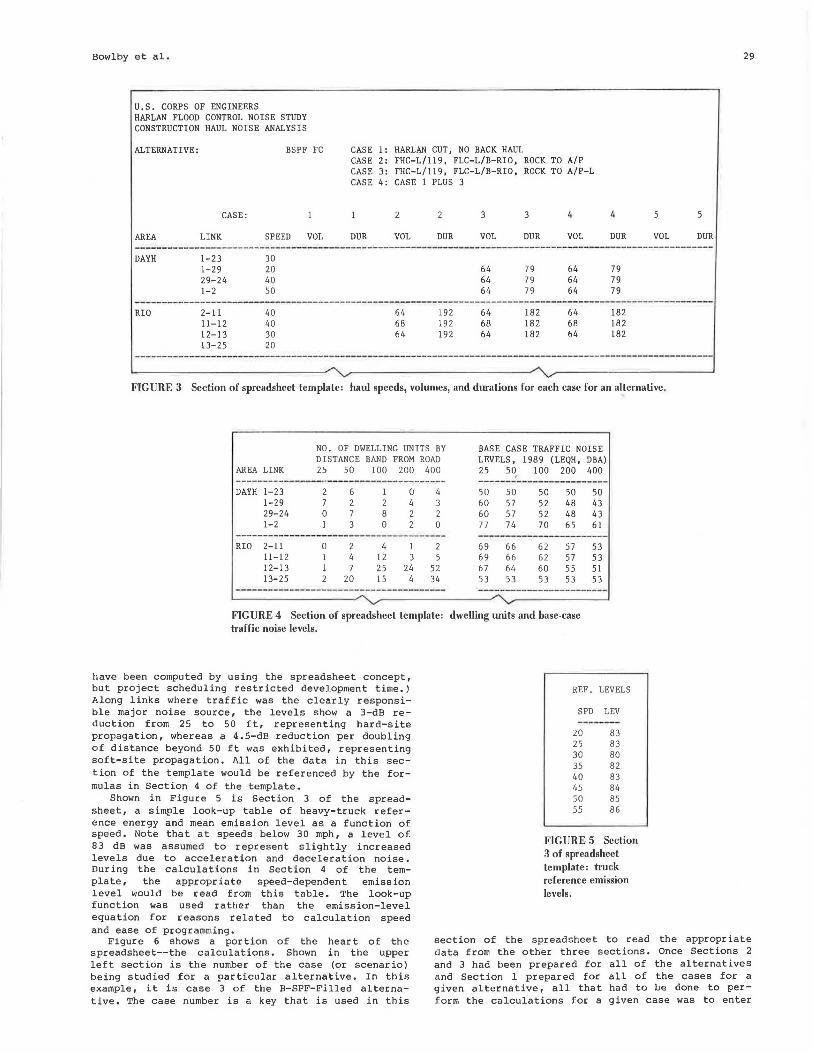
Figure 3 shows a portion of Section 1 of the spreadsheet for the B-SPF-Filled alternative. Note that link names (LINK) consist of the node numbers at both ends of a link and that the links were seg­regated by geographic location (AREA). The speeds along each link (SPEED) were assumed to be the same for all scenarios and alternatives, although these data would be easily changed variables. The rest of the columns of this section of the template are for entry of haul traffic hourly flow rates (VOL) and activity durations in weeks (DUR) for each scenario or case to be studied for each alternative. The VOL and DUR values were developed externally for the ap­propriate links on the basis of data on the amount of material to be moved, location of borrow or dis­posal sites, and construction sequencing. These values were then simply entered into the correspond­ing cells of the spreadsheet template for that al­ternative.

Figure 4 gives a portion of Section 2 of the spreadsheet. The data in this section remained the same for all of the alternatives. On the left, again, links are identified by node numbers. In the center, the number of dwelling uni ts is listed by distance band: these data were collected from maps and field reviews. To the right are the base-case daytime hourly traffic noise levels for the analysis year 1989 as a function of distance from the link. These data were either externally computed by using the FHWA model nomograph or assumed based on the ex­isting noise level field survey. (The data could

Bowlby et al.

U.S. CORPS OF ENGINEERS HARLAN FLOOD CONTROL NOISE STUDY CONSTRUCTION HAUL NOISE ANALYSIS

ALTERNATIVE:

AREA

DAYH

CASE:

LINK

1-23 1-29 29-24 1-2

BSPF

SPEED

30 20 40 50

FC CASE 1: CASE 2: CASE 3: CASE 4:

VOL DUR

HARLAN CUT, NO BACK HAUL FHC-L/119, FLC-L/B-RIO, ROCK TO A/P FHC-L/119, FLC-L/B-RIO, ROCK TO A/P-L CASE 1 PLUS 3

2 2

VOL DUR

3

VOL

64 64 64

3

DUR

79 79 79

4

VOL

64 64 64

4

DUR

79 79 79

5

VOL

---------------------------------------------------------------------RIO 2-11

11-12 12-13 13-25

40 40 30 20

--------------------

64 68 64

192 192 192

64 68 64

182 182 182

64 68 64

182 182 182

FIGURE 3 Section of spreadsheet template: haul speeds, volumes, and durations for each case for an alternative.

NO. OF DWELLING UNITS BY DISTANCE BAND FROM ROAD

AREA LINK 25 50 100 200 400 ------------ · ------------------DAYH 1-23 2 6 1 0 4

1-29 7 2 2 4 3 29-24 0 7 8 2 2 1-2 1 3 0 2 0

----·--- --------------------------RIO 2-11 0 2 4 1 2

11-12 4 12 3 s 12-13 7 2S 24 S2 13-25 2 20 lS 4 34

-------------------------------FIGURE4 Section of spreadsheet template: traffic noise levels.

have been computed by using the spreadsheet concept, but project scheduling restricted development time.) Along links where traffic was the clearly responsi­ble major noise source, the levels show a 3-dB re­duction from 25 to 50 ft, representing hard-site propagation, whereas a 4.5-dB reduction per doubling of distance beyond 50 ft was exhibited, representing soft-site propagation. All of the data in this sec­tion of the template would be referenced by the for­mulas in Section 4 of the template.

BASE CASE TRAFFIC NOISE LEVELS, 1989 (LEQH, OBA) 25 50 100 200 400

' -~--~-----------------50 50 50 50 50 60 57 52 48 43 60 S7 52 48 43 77 74 70 6S 61

69 66 62 S7 S3 69 66 62 57 53 67 64 60 SS Sl 53 S3 53 S3 S3 -~------~---~----

dwelling units and base-case

REF. LEVELS

SPD LEV -----

20 83 2S 83 30 80 3S 82 40 83 45 84 50 8S 55 86

FIGURE 5 Section 3 of spreadsheet template: truck reference emission levels.

29

5

DUR

Shown in Figure 5 is Section 3 of the spread­sheet, a simple look-up table of heavy-truck refer­ence energy and mean emission level as a function of speed. Note that at speeds below 30 mph, a level of 8 3 dB was assumed to represent slightly increased levels due to acceleration and deceleration noise. During the calculations in Section 4 of the tem­plate, the appropriate speed-dependent emission level would be read from this table. The look-up function was used rather than the emission-level equation for reasons related to calculation speed and ease of programming.

Figure 6 shows a portion of the heart of the spreadsheet--the calculations. Shown in the upper left section is the number of the case (or scenario) being studied for a particular alternative. In this example, it is case 3 of the B-SPF-Filled alterna­tive. The case number is a key that is used in this

section of the spreadsheet to read the appropriate data from the other three sections. Once Sections 2 and 3 had been prepared for all of the alternatives and Section 1 prepared for all of the cases for a given alternative, all that had to be done to per­form the calculations for a given case was to enter

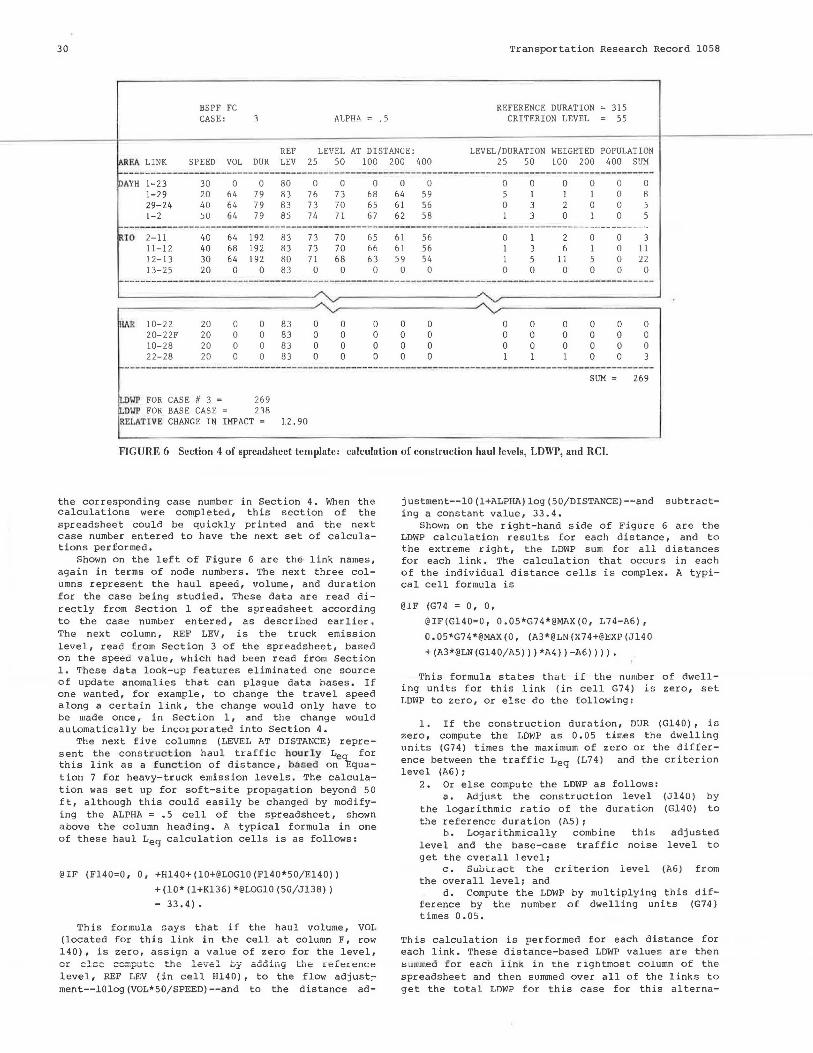
30 Transportation Research Record 1058

BSPF FC REFERENCE DURATION 315 CASE: ALPHA .s CRITERION LEVEL 55

REF LEVEL AT DISTANCE: LEVEL/DURATION WEIGHTED POPULATION AR EA LINK SPEED VOL DUR LEV 2S so 100 200 400 25 so 100 200 400 SUM ~-----------------------------·----------·-· -·---------·--·-----------------------PAYH 1-23 30 0 0 80 0 0 0 0 0 0 0 0 0 0 0

1-29 20 64 79 83 76 73 68 64 S9 s 1 1 1 0 8 29-24 40 64 79 83 73 70 65 61 56 0 3 2 0 0 s 1-2 so 64 79 8S 74 71 67 62 58 3 0 1 0 5

~-------------,-------------------------------------- -------------IRIO 2- 11 40 64 192 83 73 70 65 61 S6 0 1 2 0 0 3

11- 12 40 68 192 83 73 70 66 61 S6 1 3 6 1 0 11 12- 13 30 64 192 80 71 68 63 59 54 1 5 11 5 0 22 13-25 20 0 0 83 0 0 0 0 0 0 0 0 0 0 0

----------------------- ----------------------------------------------------- --

lAR 10- 22 20- 22F 10-28 22-28

20 20 20 20

0 0 0 0

0 0 0 0

WP FOR CASE II 3 = 269 DWP FOR BASE CASE 238

83 83 83 83

REL.ATtVE CHANGE IN IMPACT 0 12.90

0 0 0 0

0 0 0 0

0 0 0 0

0 0 0 0

0 0 0 0

0 0 0

0 0 0

0 0 0 1

0 0 0 0

0 0 0 0

0 0 0 3

SUM = 269

FIGURE 6 Section 4 of spreadsheet template: calculation of construction haul levels, LDWP, and RCI.

the corresponding case number in Section 4. When the calculations were completed, this section of the spreadsheet could be quickly printed and the next case number entered to have the next set of calcula­tions performed.

Shown on the left of Figure 6 are the link names, again in terms of node numbers. The next three col­umns represent the haul speed, volume, and duration for the case being studied. These data are read di­rectly from Section 1 of the spreadsheet according to the case number entered, as described earlier. The next column, REF LEV, is the truck emission level, read from Section 3 of the spreadsheet, based on the speed value, which had been read from Section 1. These data look-up features eliminated one source of update anomalies that can plague data bases. If one wanted, for example, to change the travel speed along a certain link, the change would only have to be made once, in Section 1, and the change would automatically be incorporated into Section 4.

The next five columns (LEVEL AT DISTANCE) repre­sent the construct i on haul traffic hourly Leq for this link as a functio n of distance, based on Equa­tion 7 for heavy-truck emission levels. The calcula­tion was set up for soft-site propagation beyond 50 ft, although this could easily be changed by modify­ing the ALPHA = • 5 cell of the spreadsheet, shown a bove the column heading. A typical formula in one of these haul Leq calculation cells is as follows:

@IF (Fl40=0, 0, +Hl40+(10+@LOG10(Fl40*50/ El40))

+(10*(l+Kl36)*@LOG10(50/ Jl38)) - 33.4).

This formula says that if the haul volume, VOL (located for this link in the cell at column F, row 140), is zero, assign a value of zero for the level,

level, REF LEV (in cell Hl40), to the flow adjust;­ment--10log (VOL*50/SPEED)--and to the distance ad-

justment--lO(l+ALPHA)log(SO/DISTANCE)--and subtract­ing a constant value, 33.4.

Shown on the right-hand side of Figure 6 are the LDWP calculation results for each distance, and t o the extreme right, the LDWP sum for all distances for each link. The calculation that occurs in each of the individual distance cells is complex. A typi­cal cell formula is

@IF (G74 = 0, 0,

@IF(Gl40=0, 0.05*G74*@MAX(O, L74-A6),

0. 05*G74*@MAX (0, (A3*@LN (X74+@EXP (Jl40

+(A3*@LN(Gl40/ AS)))*A4))-A6)))).

This formula states thal if the number of dwell­ing units for this link (in cell G74) is zero, set LDWP to zero, or else do the following:

1. If the construction duration, DUR (Gl40), is zero, compute the LDWP as 0.05 times the dwelling un i ts (G74) times the maximum of zero or the differ­ence between the traffic Leq (L74) and the criterion level (A6);

2 . Or else compute the LDWP as follows: a. Adjust the construction level (Jl40) by

the logarithmic ratio of the duration (Gl40) to the reference duration (AS) ;

b. Logarithmically combine this adjusted level and the base-case traffic noise level to get the overall level;

c. Suutract ~ne cri~erion level (A6J from the overall level; and

d. Compute the LDWP by multiplying this dif­ference by the number of dwelling units (G74) times 0.05.

Th is calculation is performed for each distance for each link. These distance-based LDWP values are then sununea for each link in the rightmost column of the spreadsheet and then summed over all of the links t o get the total LDWP for this case for this al terna-

Bowlby et al.

tive (shown as 269 in the bottom right of Figure 6) • Finally, the RCI for this case is computed, as shown in the lower left of the figure. In this example, this particular hauling scenario (Case 3) for alter­native B-SPF-Filled will cause a 12,9 percent in­crease in the LDWP over the base case of 1989 traf­fic.

Again, once Sections 1-3 were prepared, all that had to be done to compute the RCI for a given case for a given alternative was to change the case num­ber at the top of Section 4. In this manner, the many cases could be quickly analyzed and the results compiled and evaluated.

SUMMARY AND CONCLUSIONS

To assist the Corps of Engineers in assessing the construction haul-noise impact of a series of flood control project alternatives, a technique was devel­oped based on a modification to the LWP technique to account for constru~tidn haul activity duration. The resulting parameter was the LDWP.

By computing an LDWP for a base case of no con­struction hauling, where the major noise source was generally traffic, and computing an LDWP for the duration-adjusted construction haul-noise levels combined with the regular traffic noise levels, the relative change in impact (RCI) could be determined for different haul scenarios for each proposed al­ternative. The analysis techniq11~ produced aggregate impact values for comparing alternatives as well as disaggregate details on the link-by-link impacts that could be used subsequently in mitigation strat­egy development.

The technique was implemented with a complex microcomputer spreadsheet template that permitted easy data entry, rapid calculation of impacts, and immediate formatted presentation of results. The spreadsheet included several sections of data for each project alternative that were accessed by the calculations section by using look-up type func­tions. Developme'nt of the spreadsheet template was

~somewhat time-consuming and not very amenable to easy modification of the template structure. How­ever, use of the template, once developed, was sim­ple and fast, and permitted many different scenarios to be easily analyzed.

The analysis procedure, then, involved setting up the first section of each template for each alterna­tive and running the calculations in the last sec­tion of the template for each case for each alterna­tive. The resultant spreadsheets were printed after each 'recalculation. The RCI values were then tabu­lated for all of the cases for each alternative, permitting an evaluation of the relative impacts as input into the environmental assessment.

ACKNOWLEDGMENTS

The authors express their appreciation to the u.s. Arm~ Corps of Engineers, Nashville District, for

31

acting as primary funding source for this project. They also thank MCI Consulting, Inc., which serven as the prime contractor to the Corps and which was responsible for developing the haul scenarios and construction scheduling. Chuck Higgins served as principal investigator for MCI.

REFERENCES

1. Section 202 Harlan Flood Reduction Study: Plan Formulation Package. u.s. Army Corps of Engi­neers, Nashville, Tenn., 1984.

2. Procedures for Abatement of Highway Traffic Noise and Construction Noise. 23 CFR Part 772, Federal Register, Vol. 47, No. 131, pp. 29653-29657, July 8, 1982.

3. Report of Field Review--Highway Traffic Noise I•npa"bt Identification and Mitigation Decision­making Processes. FHWA, U.S. Department of Transportation, June 1982.

4. P.D. Schomer and B. Homans. Construction Noise: Specification, Control, Measurement and Mitiga­tion. Technical Report E-53. Construction Engi­neering Research Laboratory, Champaign, Ill., 1975.

5. SAE Recom.~ended Practice: Measurement Procedure for Determining a Representative Sound Level at a Construction Site Boundary Location. SAE J 184. Society of Automotive Engineers, Warr en­dale, Pa., 1975.

6. B.A. Kugler, D.E. Commins, and W.J. Galloway. Highway Noise: A Design Guide for Prediction and Control. NCHRP Report 174. TRB, National Research Council, Washington, D.C., 1976.

7. J .A. Reagan and c. Grant. Highway Construction Noise: Measurement, Prediction and Mitigation. FHWA, u.s. Department of Transportation, 1974.

8. w. Bowlby and L.F. Cohn. Highway Construction Noise--Environmental Assessment and Abatement, Vol. 4: user's Manual for FHWA Highway Con­struction Noise Computer Program, HICNOM. Van­derbilt University Report VTR 81-2. FHWA, u.s. Department of Transportation, 1982.

9. Background Document for Final Interstate Rail Carrier Noise Emission Regulation: Source Stan­dards. Report EPA 550/9-79-210. U.S. Environ­mental Protection Agency, 1979.

10. T.M. Barry and J.A. Reagan. FHWA Highway Traf­fic Noise Prediction Model. Report FHWA-RD-77-108. FHWA, u.s. Department of Transportation, 1978.

Publication of this paper sponsored by Committee on Transportation-Related Noise and Vibration.