Adebayo, Fahrmeir:

Analyzing Child Mortality in Nigeria with GeoadditiveSurvival Models

Sonderforschungsbereich 386, Paper 303 (2002)

Online unter: http://epub.ub.uni-muenchen.de/

Projektpartner

Analyzing Child Mortality in Nigeria

with Geoadditive Survival Models

Samson B. Adebayo1,2 and Ludwig Fahrmeir1

1 Department of Statistics, University of Munich, Ludwigstr. 33, D-80539 Munich,

Germany.

2 Department of Statistics, University of Ilorin, P.M.B. 1515 Ilorin, Nigeria.

Abstract

Child mortality reflects a country’s level of socio-economic development and quality

of life. In developing countries, mortality rates are not only influenced by socio-

economic, demographic and health variables but they also vary considerably across

regions and districts. In this paper, we analyze child mortality in Nigeria with

flexible geoadditive survival models. This class of models allows to measure small-

area district-specific spatial effects simultaneously with possibly nonlinear or time-

varying effects of other factors. Inference is fully Bayesian and uses recent Markov

chain Monte Carlo (MCMC) simulation. The application is based on the 1999

Nigeria Demographic and Health Survey. Our method assesses effects at a high

level of temporal and spatial resolution not available with traditional parametric

models.

Keywords child mortality, geoadditive model, Markov chain Monte Carlo, smooth-

ness priors.

1Address for correspondence.

1

1 Introduction

Child mortality and malnutrition are among the most serious socio-economic and

demographic problems in sub-Saharan African countries, and they have great impact

on future development. Demographic and Health Surveys (DHS) are designed to

collect data on health and nutrition of children and mothers as well as on fertility

and family planning. In this paper, we focus on child mortality in Nigeria, using data

from the 1999 Nigeria Demographic and Health Survey (NDHS), which was jointly

sponsored by the Nigerian National Population Commission (NPC), the United

Nations Population Fund Activities (UNPFA) and the U.S. Agency for International

Development (USAID). The main objective of the 1999 NDHS is to provide an up-to

date information on fertility and childhood mortality levels, on awareness, approval

and use of family planning methods, on breastfeeding practices, and on nutritional

level. This is intended to assist policy makers and administrators in evaluating and

designing programmes, and to develop strategies for improving health and family

planning services in Nigeria which in turn should reduce childhood mortality levels.

The 1999 NDHS includes information on survival time of respondent’s children,

who were born 3 years before the survey. This permits calculation of various child

mortality rates such as neonatal, post-neonatal and infant mortality rates. Tables 1

and 2 show child mortality rates stratified by regions and districts (states) in Nigeria

respectively. The geographical information given in Table 1 is highly aggregated

and may therefore conceal local and district specific effects. Moreover, there is no

adjustment for other covariates, which may lead to wrong conclusions. On the other

hand, raw mortality rates stratified by districts in Table 2 strongly depend on the

2

Table 1: Frequency of child mortality by regions in Nigeria.

Region No of deaths No of children Rel. freq.

North East 104 790 0.132North West 61 669 0.091South East 63 651 0.097South West 60 745 0.081Central 54 697 0.078

Total 342 3552

sample and may be rather unstable. Figure 1 shows the geographical location of

the districts (states) in Nigeria. The geographical distribution of child mortality is

shown in Figure 2, which conveys a similar impression as Table 2. Some kind of

spatial smoothing will be needed to stabilize rates observed in the sample.

1

2

3

4

5

6

7

8

9

10

11

12

13

14

15

16

17

18

19

20

21

2223

24

2526

2728

29

30

31

32

33

34

35

36

37

Figure 1:Map of Nigeria showing districts ”in numbers”.

Classical parametric regression models for analyzing child mortality or survival have

severe problems with estimating small area effects and simultaneously adjusting for

other covariates, in particular when some of the covariates are nonlinear or time-

varying. Usually a very high number of parameters will be needed for modelling

3

Table 2: Geographical distribution of child mortality by districts in Nigeria.

Number District No of deaths No of children Rel. freq.

1 Akwa-Ibom 29 213 0.1362 Anambra 5 68 0.0743 Bauchi 25 153 0.1634 Edo 13 99 0.1315 Benue 7 106 0.0666 Borno 2 68 0.0297 Cross River 2 56 0.0368 Adamawa 12 70 0.1719 Imo 4 65 0.06210 Kaduna 14 152 0.09211 Kano 54 318 0.17012 Katsina 24 213 0.11313 Kwara 5 72 0.06914 Lagos 14 132 0.10615 Niger 12 111 0.10816 Ogun 6 122 0.04917 Ondo 5 66 0.07618 Oyo 7 131 0.05319 Plateau 7 90 0.07820 Rivers 5 57 0.08821 Sokoto 16 96 0.16722 Abia 5 71 0.07023 Delta 5 99 0.05124 Enugu 4 46 0.08725 Jigawa 7 95 0.07426 Kebbi 6 85 0.07127 Kogi 5 104 0.04828 Osun 4 76 0.05329 Taraba 3 74 0.04130 Yobe 10 110 0.09131 Bayelsa 0 16 0.00032 Ebonyi 9 59 0.15333 Ekiti 6 20 0.30034 Gombe 6 46 0.13035 Nassarawa 3 43 0.07036 Zamfara 1 123 0.00837 FCT-Abuja 0 27 0.000

Total 342 3552

4

0 0.3

Figure 2: Coloured map of Nigeria showing the geographical distributions of mortality rates

in proportion. Constructed from Table 2.

purposes, resulting in rather unstable estimates with high variance. Therefore, flex-

ible semiparametric approaches are needed which allow one to incorporate small-area

spatial effects, nonlinear or time-varying effects of covariates and usual linear effects

in a joint model.

In this paper, we apply Bayesian geoadditive survival models which can deal with

these aspects by introducing appropriate smoothness priors for spatial and non-

linear effects. Because survival time of children is measured in months, we rely

on discrete-time survival models, which are reviewed in Fahrmeir and Tutz (2001,

ch.9). Bayesian inference uses recent Markov chain Monte Carlo (MCMC) simu-

lation techniques, described in Fahrmeir and Lang (2001a, b), Lang and Brezger

(2002), and implemented in the open domain software BayesX available from

http://www.stat.uni-muenchen.de/~lang/BayesX. In a related work, Crook,

5

Knorr-Held and Hemingway (2002) apply a geoadditive probit model for analyz-

ing time to event data in a medical context. We prefer a geoadditive survival model

with a logit link because of better interpretability and the possibility to compute

posteriors of odds ratios directly, rather than using a plug-in estimate.

Previous studies on child mortality have focused on various socio-economic, demo-

graphic or health factors available in specific data sets, but have mostly neglected

spatial aspects, see for instance Mosley and Chen (1984), Miller et al. (1992), Boerma

and Bicego (1992), Guilkey and Riphahn (1997), and Berger, Fahrmeir and Klasen

(2002).

In Section 2 we discuss the study and data set, while Section 3 describes geoadditive

discrete-time survival models. Section 4 contains the statistical analysis of child

mortality in Nigeria, and the results are discussed in Section 5. Concluding remarks

are given in Section 6.

2 Study and Data

A recent publication by the Commonwealth Secretariat showed that Nigeria, one

of the most populous countries in the world with a population of over 120 million

people, in spite of its abundant mineral resources is one of the poorest countries in

the world with an average GNP per capita income of $260. Less than 10 per cent of

Nigerians are employed by the government and big organizations. Recently United

Nations human right watch reported on BBC that the Niger Delta, consisting of the

districts Delta, Edo, River, Bayelsa, Akwa-Ibom and Cross River (see Figure 1 and

Table 2), where the largest proportion of Nigerian petroleum is being drilled, is less

6

Table 3: Descriptive information about covariates according to some socio-economic char-

acteristics.

Variable Frequency (%) Coding

Place of ResidenceUrban 820 (29.23) 1Rural 1985 (70.77) -1SexMale 1427 (50.87) 1Female 1378 (49.13) -1Tetanus injection during pregnancy?Tetanus injection received 1549 (55.21) 1No Tetanus injection received 1256 (44.79) -1Mother’s educational attainment

At most primary 2042 (72.80) 1Beyond primary 763 (27.20) -1Mother assisted at birth or not?Assisted 2401 (85.61) 1Not assisted 404 (14.39) -1Place of deliveryHospital 1034 (36.88) 1Others 1771 (63.12) -1Preceding birth intervalLong birth interval 1968 (70.16) 1Short birth interval 837 (29.84) -1At least one antenatal visit?Antenatal visit 1618 (57.69) 1No antenatal visit 1187 (43.31) -1Mother’s age at birthLess than 22 years 567 (20.21) 122-35 years 1861 (66.35) 2Greater than 35 years 377 (13.44) 3(-1)

7

developed. There is lack of social amenities and good roads, education facilities are

poor, and the unemployment rate is high.

This paper is based on data available from the 1999 NDHS. It is a nationally rep-

resentative survey of women of reproductive age (15-49 years) and their children

below the age of three years before the survey. Data on childhood mortality are

contained in the birth history section of the Women’s Questionnaire, see National

Population Commission[Nigeria](2000). Questions include child bearing experience

such as total number of sons and daughters alive or dead. For all children who had

died, the respondent was asked of their age at death which was recorded in months.

Since diarrhea and respiratory illness are common causes of child mortality in Nige-

ria, data were also collected on child’s health such as evidence of diarrhea, cough,

fever and childhood vaccination coverage.

Data were collected on 3552 children from women of reproductive age. A data set

was constructed from children’s individual records of the 1999 NDHS. Each record

represents a child, and consists of survival information as well as a large number of

covariates that may influence child mortality. Crude mortality rates stratified by

districts are displayed in Table 2 and Figure 2. For each child, the data set contains

survival information in the following form: Either a child is still alive at the time

of survey, i.e. it has survived the first 36 months, or, it has died, then its survival

time is given in months. Factors such as mother’s educational attainment, sex of

the child, current working status of mother, assistance at delivery and evidence of

illness two weeks prior to the survey, etc. were included in data analysis at the

preliminary level. However, some of these covariates were not significant and were

8

removed at a later stage. Also, some of the covariates had missing observations.

We deleted records of children with missing observations from the data, resulting in

2805 children with complete information. Table 3 gives some descriptive statistics

on these covariates.

From previous studies, e.g. Berger et al. (2002), it is known that breastfeeding

is an important factor. To assess this effect we generated a time-varying indicator

variable that takes the value 1 in the months a child is breastfed, and 0 otherwise.

3 Geoadditive Discrete-Time Survival Model

Let T ∈ {1, . . . , k = 36} denote survival time in month. Then T = t denotes failure

time (death) in month t. Suppose xit is a vector of covariates up to month t, then

λ(t|xit) is the discrete hazard function given by

λ(t|xit) = P (T = t|T ≥ t, xit) (3.1)

as the conditional probability of death in month t given that the child has reached

month t, and the discrete survivor function for surviving time t is given by

S(t|xit) = P (T > t|xit) =k∏

t=1

(1 − λ(t|xit)). (3.2)

Survival information on each child is recorded as (ti, δi), i = 1, · · · , 2805, ti ∈

{1, · · · , 36} is the observed life time in months, and δi is the survival indicator

with δi=1 if child i is dead and δi=0 if it is still alive. Thus for δi=1, ti is the age

of the child at death, and for δi=0, ti is the current age of the child at interview.

Discrete-time survival models can be cast into the framework of binary regression

9

models by defining binary event indicators yit, t = 1, . . . , T with

yit =

⎧⎪⎪⎪⎨⎪⎪⎪⎩

1 : ift = tiandδi = 1

0 : ift < ti.

Then hazard function (3.1) for child i can then be written as a binary response

model

P (yit|xit) = h(ηit), (3.3)

where xit are the covariate processes for child i, h is an appropriate response or link

function, and the predictor ηit is a function of the covariates.

Common choices for discrete survival models of the form (3.3) are the grouped Cox

model and logit or probit model. Practical experience and theoretical arguments

show that results and inferential conclusions are rather similar for these models

when the number of time intervals is moderate or large. Crook et al. (2002) apply a

probit model for computational reasons. In this paper, we prefer a logit form. The

conventional model is then

P (yit = 1|ηit) =eηit

1 + eηit(3.4)

with partially linear predictor

ηit = f0(t) + x′itγ, (3.5)

where f0(t) is the baseline effect and γ are fixed effect parameters. The main reason

for preferring a logit model is interpretability: The models (3.4) and (3.5), can be

equivalently expressed as

P (yit = 1|xit)

P (yit = 0|xit)= exp(f0(t)) exp(x′

itγ), (3.6)

10

i.e. as a multiplicative model for the odds. Another advantage is that we can draw

posterior odds ratio samples directly via the relation (3.6) rather than using a plug-

in estimate for the right hand side of (3.6). Furthermore, the DIC for logit models

are smaller than for the corresponding probit models (though this is not reported

in Table 4). We consider the model (3.4), (3.5) or (3.5), (3.6) as the basic form of

semiparametric survival models. The baseline hazard effect f0(t), t = 1, 2, . . . is an

unknown, usually non-linear function of t to be estimated from the data. Treating

the effects f0(t), t = 1, 2, . . . as separate parameters usually gives either very un-

stable estimates or may even lead to divergence of the estimation procedure. In a

purely parametric framework the baseline hazard is therefore often modelled by a

few dummy variables dividing the time-axis t into a number of relatively small seg-

ments or by some low order polynomial. In general it is difficult to correctly specify

such parametric functional forms for the baseline effects in advance. Nonparametric

modelling based on some qualitative smoothness restriction offers a more flexible

solution to explore unknown dynamic patterns in f0(t). The effects γ of covariates

are assumed to be fixed and time-constant.

In many situations, and in particular in our application, the assumption of fixed

covariate effects is too restrictive. First, the effects of some covariates may vary over

time or may be nonlinear. Secondly, as in our study, modelling of spatial effects with

separate fixed effects for all the districts will introduce too many parameters and

correlation between neighboring districts is ignored. Therefore, the semiparametric

predictor (3.5) is generalized to a geoadditive predictor

ηit = f0(t) + z′itf(t) + fspat(si) + v′itγ. (3.7)

11

Here the effects f(t) of the covariates in zit are time-varying, vit comprises covariates

with an effect γ that remains constant over time, and fspat(si) is the nonlinear

effect of district si ∈ {1, . . . , S}, where child i lives. Also the time-dependent effect

function f(t) will be modelled non-parametrically. We may further split up spatial

effects fspat into spatially correlated (structured) and uncorrelated (unstructured)

effects as

fspat(si) = fstr(si) + funstr(si).

A rationale behind this is that a spatial effect is a surrogate of many unobserved

influential factors, some of which may obey a strong spatial structure and others

may only be present locally.

To estimate smooth effect functions and model parameters, we use a fully Bayesian

approach, as developed in Fahrmeir and Lang (2001a, b) and, Lang and Brezger

(2002). For all parameters and functions we have to assign appropriate priors. For

fixed effect parameters γ we assume diffuse priors. For the baseline effect f0(t) and

time-varying effects f(t) we assume Bayesian P-spline priors as in Lang and Brezger

(2002). The basic assumption behind the P-splines approach (Eilers and Marx, 1996)

is that the unknown smooth function f can be approximated by a spline of degree

l defined on a set of equally spaced knots xmin = ζ0 < ζ1 < . . . < ζs−1 < ζs = xmax

within the domain of x. Such a spline can be written in terms of a linear combination

of m = s + l B-spline basis functions Bt, i.e.

f(x) =m∑

t=1

βtBt(x), (3.8)

where β = (β1, · · · , βm) corresponds to the vector of unknown regression coefficients.

Regression splines depend on the choice of the number of knots and their placement.

12

With too few knots the resulting spline may not be flexible enough to capture the

variability of the data, conversely with too many knots estimated curves may tend

to overfit the data, resulting in too rough functions. The idea of P-splines is to

choose a generous number of knots and to regularize the problem by smoothness

assumptions on the coefficients. Within a Bayesian context, smoothness is achieved

by a first or a second order random walk model

βt = βt−1 + ut, βt = 2βt−1 − βt−2 + ut (3.9)

for the regression coefficients, with Gaussian errors ut ∼ N(0, τ 2). A first order

random walk penalizes abrupt jumps βt − βt−1 between successive states and a

second order random walk penalizes deviations from the linear trend 2βt−1 − βt−2.

The amount of smoothness is controlled by the variance τ 2.

For the structured spatial effects fstr(s), we choose a Gaussian Markov random field

prior, which is common in spatial statistics. It is given as

fstr(s)|fstr(t) t �= s, σ2 ∼ N

⎛⎝∑

t∈∂s

fstr(t)/Ns, σ2/Ns

⎞⎠ , (3.10)

where Ns is the number of adjacent sites and t ∈ ∂s denotes that site t is a neighbour

of site s. Thus the (conditional) mean of fstr(s) is an average of function evaluations

fstr(t) of neighbouring sites t. Again σ2 controls the amount of spatial smoothness.

Unstructured spatial effects are i.i.d. random effects, i.e.

funstr(s) ∼ N(0, φ2).

In order to be able to estimate the smoothing parameters τ 2, σ2 and φ2 simultane-

ously with all the unknown smooth functions, highly dispersed but proper hyper-

priors are assigned to them. Hence for all variance components, an inverse gamma

13

distribution with hyperparameters a and b is chosen, e.g. τ 2 ∼ IG(a, b). Standard

choices for the hyperparameters are a=1 and b=0.005 or a=b=0.001. The latter

choice is closer to Jeffrey’s noninformative prior, but we have investigated sensitiv-

ity to this choice in our application.

Fully Bayesian inference is based on the posterior distribution of the model pa-

rameters, which is not of a known form. Therefore, MCMC sampling from full

conditionals for nonlinear effects, spatial effects, fixed effects and smoothing pa-

rameters is used for posterior analysis. For nonlinear and spatial effects, we applied

Metropolis-Hastings algorithms based on conditional prior proposals, first suggested

by Knorr-Held (1999) in the context of state space models, and iteratively weighted

least squares (IWLS) proposals, suggested in Brezger and Lang (2002) as an ex-

tension of Gamerman (1997); see also the related work by Knorr-Held and Rue

(2002). Both sampling schemes gave rather coherent results; we rely hereon the

IWLS proposal, implemented in BayesX.

An essential task of the model building process is the comparison of a set of plausible

models, for example to rate the impact of covariates and to assess if their effects

are time-varying or not, or to compare geoadditive models with simpler parametric

alternatives. The comparison of models intends to select the model that takes all

relevant structure into account while remaining parsimonious. A model criterion

should therefore aim at a trade off between goodness of fit and model complex-

ity. We routinely use the recently proposed Deviance Information Criterion DIC

(Spiegelhalter et al., 2002), given as

DIC(M) = D(M) + pD. (3.11)

14

Here the posterior mean of the deviance D(M), which is a measure for goodness

of fit of model M, is penalized by the effective number of model parameters pD,

measuring the complexity of the model.

4 Data Analysis

Based on previous work in Berger et al. (2002) and on preliminary exploratory

analysis we decided to include the following covariates:

15

bft breastfeeding indicator, with bft=1 if a child is breastfed in month

t, 0 otherwise.

magb mother’s age at birth of the child (in years)

s district in Nigeria

w vector of binary covariates consisting of

place of residence: urban or rural (reference category),

child’s sex: male or female (reference category),

mother received tetanus injection during pregnancy or not: tetanus

or no tetanus (reference category),

mother’s educational attainment: at most primary education or sec-

ondary and above (reference category),

mother received assistance at delivery: assisted or not assisted (ref-

erence category),

place of child delivery: hospital or others (reference category),

preceding birth interval: long birth interval i.e. ≥ 24 months or

short interval i.e. < 24 months (reference category),

at least one antenatal visit during pregnancy?: antenatal or no

antenatal (reference category).

All covariates are effect coded.

The response variable is

yit =

⎧⎪⎪⎪⎨⎪⎪⎪⎩

1 : if child i dies in month t

0 : if child i survives.

16

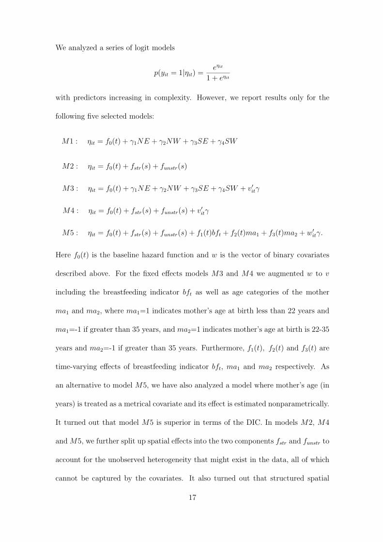
We analyzed a series of logit models

p(yit = 1|ηit) =eηit

1 + eηit

with predictors increasing in complexity. However, we report results only for the

following five selected models:

M1 : ηit = f0(t) + γ1NE + γ2NW + γ3SE + γ4SW

M2 : ηit = f0(t) + fstr(s) + funstr(s)

M3 : ηit = f0(t) + γ1NE + γ2NW + γ3SE + γ4SW + v′itγ

M4 : ηit = f0(t) + fstr(s) + funstr(s) + v′itγ

M5 : ηit = f0(t) + fstr(s) + funstr(s) + f1(t)bft + f2(t)ma1 + f3(t)ma2 + w′itγ.

Here f0(t) is the baseline hazard function and w is the vector of binary covariates

described above. For the fixed effects models M3 and M4 we augmented w to v

including the breastfeeding indicator bft as well as age categories of the mother

ma1 and ma2, where ma1=1 indicates mother’s age at birth less than 22 years and

ma1=-1 if greater than 35 years, and ma2=1 indicates mother’s age at birth is 22-35

years and ma2=-1 if greater than 35 years. Furthermore, f1(t), f2(t) and f3(t) are

time-varying effects of breastfeeding indicator bft, ma1 and ma2 respectively. As

an alternative to model M5, we have also analyzed a model where mother’s age (in

years) is treated as a metrical covariate and its effect is estimated nonparametrically.

It turned out that model M5 is superior in terms of the DIC. In models M2, M4

and M5, we further split up spatial effects into the two components fstr and funstr to

account for the unobserved heterogeneity that might exist in the data, all of which

cannot be captured by the covariates. It also turned out that structured spatial

17

effects are not statistically significant in the decomposition, while the total spatial

effects (fstr +funstr) are significant. Therefore, when interpreting results, we discuss

only total spatial effects.

To estimate f0(t), f1(t), f2(t) and f3(t) we chose Bayesian P-splines priors, and

Markov random field priors (3.10) for fstr(s).

We based Bayesian model selection on the Deviance Information Criterion (DIC)

of Spiegelhalter et al. (2002). Models with the smallest DIC and with adequate

information about the covariates were selected. All analyses were carried out with

BayesX - version 0.9 (Brezger, Kneib and Lang, 2002), a software for Bayesian

inference based on Markov Chain Monte Carlo simulation techniques.

We also investigated sensitivity to the choice of different hyperparameter values for

the five selected models. For all the nonlinear effects of f0, f1, f2 and f3, changing

the values of a and b has no impact on these effects. However, for district-specific

spatial effects, results are more stable with a = 1, b = 0.005 and a = b = 0.001 than

with other values investigated.

5 Discussion of Results

We start with a discussion of the results for spatial effects. Comments on the baseline

effect f0(t), which is included in all five models and has rather similar patterns, and

on covariate effects follow then.

Models M1 and M3 are of the basic conventional form (3.6) and assume usual fixed

effects for regions and covariates. For model M1 the geographical pattern of the

five regions in Figure 3a reflects the crude mortality rates of Table 1. Inclusion of

18

covariates in model M3 improves the model in terms of deviance and DIC consid-

erably. Note that the spatial pattern changes considerably compared to model M1

after adjusting for covariates (Figure 3b). Yet the aggregation of the 37 districts

of Nigeria into 5 regions is too coarse for a thorough discussion of spatial results,

and may even lead to misleading conclusions. This can already be seen from the

district-specific pattern in Figure 3c obtained from model M2. It is obvious, that

spatial effects of districts within the same region can vary a lot. This implies that

interpretations for regions drawn from Figure 3b will be strongly biased or wrong

for some of the districts within a region. After adjusting for the same covariates as

in model M3, the corresponding geographical pattern of district-specific effects in

model M4 shown in Figure 3d is still comparable to the one in Figure 3c, although

the DIC value in Table 4 shows a clear improvement. This means that nonpara-

metric Bayesian modelling of small-area effects is also more robust with respect to

correct adjustment by covariates than the traditional parametric approach. Figures

3e and 3f are significance maps (at 80% level), showing districts with positively

significant (white), negatively significant (black) and nonsignificant effects (grey).

These maps again confirm that there is a change in spatial pattern when moving on

from model M2 to model M3, but it is not dramatic.

Finally model M5 is an extended version of model M4, by allowing for time-varying

effects of breastfeeding and mother’s age at birth similarly as in Berger et al. (2002).

Further improvement is clearly indicated by the DIC in Table 4. We discuss now

the spatial effects shown in Figure 4 in more detail.

Obviously there exists a district-specific geographical variation in the level of child

19

mortality in Nigeria based on 1999 NDHS. Figure 4b reveals that significant high

child mortality rates are associated with coming from Akwa-Ibom (1), Ebonyi (32)

(in the South-East), Ekiti (33) (in the South-West), Adamawa (8) (in the Central),

Sokoto (21) (in the North-West) and Bauchi (3) (in the North-East) districts of Nige-

ria. On the other hand, Zamfara (36), Kebbi (20), Jigawa (25), Niger (15), Kaduna

(10) and Borno (6) districts are associated with significantly low child mortality

rates. There are nonsignificant spatial effects in the remaining districts including

the Federal Capital Territory - Abuja (37).

These variations may be attributable to differences in the physical environment

where a child lives, which in turn influence exposure to diseases. For instance, it

is likely that high child mortality rates in the South-Eastern region, unfortunately

where the country generates its major income from petroleum, can be attributed

to incessant oil spillage which has become almost an annual event in that part

of the country. The hazardous effect of pollution, which is an end result of oil

spillage, is a major problem in that area. For example, land pollution has hindered

the affected communities from being involved in farming. Water pollution makes

access to drinkable water, water for household use and hygienic sanitation difficult.

Together with air pollution these often result in outbreak of diseases such as diarrhea,

fever, cough, cholera, respiratory illness, etc. and food insecurity. A notable cause

of high mortality rates in North-Eastern and North-Western regions could either

be due to incessant communal, ethnic and religious clashes (e.g. in Bauchi (3) and

Adamawa (8)) or drought or both, the aftermath of which could result in shortage

of food supply and natural depopulation. The cause of high mortality rates in Ekiti

(33) district is very likely due to the fact that it is located on a lowland. Other

20

reasons could be as a result of outbreak of malaria and other natural cause(s) not

included in the data set.

Figure 5 shows from top to bottom, the nonlinear effect f0(t) of age (baseline ef-

fect) and the time-varying effects f1(t), f2(t) and f3(t) respectively, modelled and

fitted through Bayesian P-splines. Starting from a comparably high level in the first

month, the age effect declines more or less steadily until months 24 to 25 months,

where a bump appears, which is likely caused by heaping of children who died at

this age. A flexible baseline as in our approach helps to control for this heaping.

For comparison, we also applied a piecewise constant model for f0(t) with fixed

effects for the three categories t = 1, t=2 to 25 and t=26 to 36. For model M5

we obtained the follwoing posterior means (and 10%, 90% quantiles) respectively:

4.442 (3.740, 5.231), 0.236 (-0.453, 1.062) and -4.678 (-6.215, -3.394). This clearly

confirms the relatively high mortality risk in the first month. The DIC, however,

was higher than for model M5 with flexible baseline hazard. The second panel from

top displays time-varying effect of breastfeeding. It is evident that breastfeeding

only reduces mortality risk in the early months of life, while its impact beyond 4

months is either negligible or increases the risk of child mortality. This, of course,

is reasonable as breastfeeding at old age will not be sufficient to keep the child

strong, hale and healthy. A remarkable observation here is that exclusive breast-

feeding is only practiced within the first four months of live among Nigerian mothers

though exclusive breastfeeding is recommended for the first four to six months of

life (WHO/UNICEF, 1990). The third panel (from top) of the Figure shows the

time-varying effect of younger mother (< 22 years) while the fourth panel shows the

varying effect of middle-aged mother (22-35 years). Although confidence bounds

21

become quite wide at the end of the observation period, it seems that mortality

risks are reduced when the mother is older (22-35 years) and has more experience.

Table 5 displays the posterior estimates of the fixed effect parameters in model M5.

Mother’s educational attainment significantly affects the survival chances of the

child with children from educated mothers (secondary and above) having lower risks

of dying in comparison to their counterparts. Mothers that received assistance at

delivery, child delivered at the hospital and with high preceding birth intervals, have

less risks of child mortality. The interaction effect of receiving assistance at birth

and having visited (at least once) an antenatal clinic during pregnancy, reduces the

risk of child mortality (though antenatal visit on its own is not significant). All these

findings confirm the descriptive results in National Population Commission [Nigeria]

(2000). While effects of mother’s educational attainment, received assistance at birth

and delivery of the child taking place at a hospital are only significant at 80% credible

intervals, effects of long birth interval and interaction of assistance and antenatal

visit are both significant at 95% credible intervals.

Table 6 shows ratios of relative risks for the fixed effects of model M5. According

to (3.6), the ratio of relative risks of a binary covariate x ∈ {1,−1} is λ = exp(2γ).

This parameter can be sampled together with γ which is an advantage of the logit

model. The factor λ then describes the increase or decrease of the relative risk of

a child with covariate x = 1 compared to a child with x = −1, but with the same

values for the remaining factors.

22

6 Concluding Remarks

In many lifetime or mortality studies, the data contain geographical information at

a high spatial resolution. Compared to traditional parametric methods, Bayesian

geoadditive models have distinct advantages for exploring small-area spatial effects.

Of course, these spatial effects have no causal impact but careful interpretation can

help to find latent, unobserved factors which directly influence mortality rates. From

a methodological point of view, we have focused on discrete-time survival model.

Extensions to continuous-time models, such as the Cox proportional hazard model

are desirable and will be a topic of future research.

23

References

[1] Berger, U., Fahrmeir, L. & Klasen, S. (2002): Dynamic Modelling of Child Mortality

in Developing Countries: Application for Zambia. SFB 386 Discussion Paper 299,

University of Munich, Germany.

[2] Boerma, J.T. & Bicego, G.T. (1992): Preceding Birth Intervals and Child Survival:

Searching for Pathways of Influence. Studies in Family Planning 23:243-256.

[3] Brezger, A., Kneib, T. & Lang, S. (2002): BayesX - Software for Bayesian Infer-

ence based on Markov Chain Monte Carlo simulation Techniques.Available under

http://www.stat.uni-muenchen.de/~lang/BayesX.

[4] Crook, A.M., Knorr-Held, L. & Hemingway, H.(2002): Measuring Spatial Effects

in Time to Event Data: a case study using months from Angiography to Coronary

Artery Bypass Graft (CABG). (Revised for Statistics in Medicine).

[5] Eilers, H.C. & Marx, D.B. (1996): Flexible Smoothing with B-Splines and Penalties.

Statistical Science, 11(2):89-121.

[6] Fahrmeir, L. & Lang, S. (2001a): Bayesian Inference for generalized additive mixed

models on Markov random field priors. Applied Stat., 50(2):201-220.

[7] Fahrmeir, L. & Lang, S. (2001b): Bayesian Semiparametric Regression Analysis of

Multicategorical Time-Space Data. Annals of the Institute of Statistical Mathematics,

52,No 1:1-18.

[8] Fahrmeir, L. & Tutz, G. (2001): Multivariate Statistical Modelling based on Gener-

alized Linear Models (3rd ed.), Springer, New York.

[9] Gamerman, D. (1997): Efficient Sampling from the Posterior Distribution in Gener-

alized Linear Models. Statistics and Computing, 7:57-68.

[10] Guilkey, D. & Riphahn, R. (1997): The Determinants of Child Mortality in the

Philipines: Estimation of a Structural Model. Journal of Development Economics,

56(2):281-305.

24

[11] Knorr-Held, L. (1999): Conditional Prior Proposals in Dynamic Models. Scandina-

vian Journal of Statistics, 26:129-144.

[12] Knorr-Held, L. & Rue, H. (2002): On Block Updating in Markov Random Field

Models for Disease Mapping. To appear in: Scandinavian Journal of Statistics.

[13] Lang, S. & Brezger, A. (2002): Bayesian P-Splines. To appear in: Computational

and Graphical Statistics.

[14] Miller, J.E., Trussel, J., Pebley, A.R. and Vanghan, B. (1992): Birth Spacing and

Child Mortality in Bangladesh and the Phillipines. Demography 29:305-318.

[15] Mosley, W.H. and Chen, L.C. (1984): Child Survival Strategies for Research. Popu-

lation Development Review 10:25-45.

[16] National Population Commission [Nigeria] (2000): Nigeria Demographic and

Health Survey 1999. Calverton, Maryland: National Population Commission and

ORC/Macro.

[17] Spiegelhalter, D., Best, N., Carlin, B. and van der Linde, A. (2002): Bayesian Mea-

sures of Model Complexity and Fit. Journal of the Royal Statistical Society, B 64:1-34

(without discussion).

[18] World Health Organization (WHO)/UNICEF. 1990. Meeting on Breastfeeding in the

1990s: A Global Initiative. Innocenti Declaration on the Protection, Promotion and,

Support of Breastfeeding. Florence, Italy August 1. UNICEF: New York.

25

Table 4: Summary of the DIC for models M1 to M5.

Model Deviance pD DIC

M1 3725.74 19.06 3744.80M2 3677.76 34.22 3711.98M3 2169.45 29.21 2198.66M4 2119.96 44.16 2164.12M5 2074.11 52.40 2126.51

Table 5: Posterior estimates of the fixed effect parameters for model M5.

Variable mean std. error 5% 10% 90% 95%

Urban 0.001 0.094 -0.181 -0.115 0.121 0.187Male 0.047 0.072 -0.106 -0.043 0.139 0.172At most primary 0.191 0.096 -0.008 0.068 0.310 0.380Assisted -0.154 0.102 -0.363 -0.290 -0.024 0.049Hospital -0.188 0.113 -0.412 -0.349 -0.041 0.019Long birth interval -0.426 0.088 -0.623 -0.538 -0.314 -0.258Assist*antenatal -0.198 0.087 -0.375 -0.304 -0.092 -0.027

Table 6: Posterior estimates of the relative risk ratios for model M5.

Variable mean std. error 5% 10% 90% 95%

Urban 1.019 0.193 0.739 0.794 1.274 1.342Male 1.110 0.156 0.866 0.917 1.320 1.373At most primary 1.493 0.288 1.049 1.145 1.857 2.006Assisted 0.751 0.155 0.517 0.560 0.953 1.004Hospital 0.705 0.157 0.469 0.498 0.922 0.972Long birth interval 0.433 0.076 0.315 0.341 0.533 0.571Assist*antenat 0.683 0.120 0.509 0.545 0.833 0.901

26

-0.196152 0.3529330

a) Regional fixed effects in model M1

-0.429492 0.5047220

b) Regional fixed effects in model M3

-0.67059 0.6603080

c) Total spatial effects in model M2

-1.04885 1.148810

d) Total spatial effects in model M4

e) 80% Posterior probabilities (total) in model M2 f) 80% Posterior probabilities (total) in model M4

Figure 3: Coloured maps of Nigeria showing posterior means of regional fixed effects in

models M1 (top left) and M3 (top right), nonlinear (total) spatial effects in models M2

(middle left) and M4 (middle right), and maps of 80% posterior probabilities for models

M2 (bottom left) and M4 (bottom right) respectively.

27

-1.19905 1.135210

a) Total spatial effects in model M5 b) 80% Posterior probabilities (total) in model M5

Figure 4: a) Coloured map of total spatial effects and b) the corresponding map of 80%

posterior probabilities in models M5.

28

Baseline effect

time

f(tim

e)

-50

-40

-30

-20

-10

010

0 10 20 30

varying effect of breastfeeding

time

f( ti

me

)

-2-1

01

23

0 10 20 30

varying effect of mother’s age < 22

time

f( ti

me

)

0.0

0.5

1.0

1.5

0 10 20 30

varying effect of mother’s age 22-35

time

f( ti

me

)

-2.0

-1.5

-1.0

-0.5

0.0

0.5

0 10 20 30

Figure 5: Graphs of nonlinear effects from top to bottom: baseline effect, varying effect of

breastfeeding, varying effect of mother’s age < 22 years and varying effect of mother’s age

22-35 years respectively for model M5.

29