analyzing and testing the structure of china’s imports for

Master’s thesis · 30 hec · Advanced level European Erasmus Mundus Master Program: Agricultural Food and Environmental Policy Analysis (AFEPA) Degree thesis No 805 · ISSN 1401-4084 Uppsala 2013

Analyzing and Testing the Structure of China’s Imports for Cotton - A Bayesian System Approach Ruochen Wu

Analyzing and Testing the Structure of China’s Impo rts for Cotton - A Bayesian System Approach Ruochen Wu Supervisor: Sebastian Hess, Swedish University of Agricultural Sciences (SLU), Department of Economics Assistant supervisor: Yves Surry, Swedish University of Agricultural Sciences (SLU), Department of Economics Examiner: Ing-Marie Green, Swedish University of Agricultural Sciences (SLU), Department of Economics Credits: 30 hec Level: A2E Course title: Independent Project/degree in Economics E Course code: EX0537 Programme/Education: European Erasmus Mundus Master Program: Agricultural Food and Environmental Policy Analysis (AFEPA) Faculty: Faculty of Natural Resources and Agricultural Sciences Place of publication: Uppsala Year of publication: 2013 Name of Series: Degree project/SLU, Department of Economics No: 805 ISSN 1401-4084 Online publication: http://stud.epsilon.slu.se Key words: China, cotton import demand, generalized Armington Model, CDE functional form, Bayesian Bootstrap Multivariate Regression, Allen elasticities of substitution

iii

ABSTRACT

China is the biggest importer of cotton in the world, and it is of great interest to analyze its import

demand system for cotton. Noteworthy is that cotton is deemed an intermediate commodity for

textile production instead of a direct consumption one, hence this thesis adopts a two-stage cost

minimization procedure resembling the Armington Model to study China’s demand for cotton

differentiated by their countries of production with a focus on the substitution effects and weak

separability between various sources. The CDE functional form is utilized for the cost function to

generalize the Armington settings. Unlike former works, this thesis estimates the demand system

with the Bayesian Bootstrap Multivariate Regression, and report the posterior distributions of

coefficients and Allen elasticities of substitution. The results demonstrate that the CDE functional

form may still be too demanding to be completely consistent with the data. Three weak separable

structures are tested, and it can be concluded that the assumption of different separable structures

improves the consistency between the model and data to various extents. The U.S. cotton is the

least sensitive to its own price changes while the cotton from Egypt and Sudan is the most

sensitive. The overall substitution effects between various cotton import sources appear to be

relatively small.

Keywords: China, cotton import demand, generalized Armington Model, CDE functional form,

Bayesian Bootstrap Multivariate Regression, Allen elasticities of substitution

iv

TABLE OF CONTENTS

ACKNOWLEDGEMENT .............................................................................................................vi

DEDICATION ...............................................................................................................................vii

ABBREVIATIONS ......................................................................................................................viii

CHAPTER 1 – INTRODUCTION ............................................................................................1

1.1 Background..................................................................................................................1

1.2 Cotton production and import of China ...................................................................1

1.3 Problem statement......................................................................................................3

1.4 Research hypothesis....................................................................................................4

1.5 Objectives.....................................................................................................................5

1.6 Organization of the thesis...........................................................................................5

CHAPTER 2 – LITERATURE REVIEW ................................................................................6

2.1 Models for demand systems and the trade in agricultural products ......................6

2.2 Cotton markets and policies with an international perspective............................10

2.3 Cotton trade of China...............................................................................................14

2.4 Former works on demand structure in cotton trade..............................................15

2.5 Conclusion..................................................................................................................17

CHAPTER 3 – THEORETICAL AND EMPIRICAL MODELS .........................................19

3.1 Theoretical model of cotton import of China..........................................................19

3.2 The CDE functional form .........................................................................................21

3.3 Weak separability......................................................................................................22

3.4 Empirical model ........................................................................................................23

3.4.1 Model specification........................................................................................23

3.4.2 Weak separability..........................................................................................24

CHAPTER 4 – ECONOMETRIC APPROACH ...................................................................26

4.1 A brief introduction to Bayesian econometrics.......................................................26

4.1.1 Bayes Theorem..............................................................................................26

4.1.2 The Bayesian econometrics in comparison to frequentist econometrics..26

4.2 Bayesian bootstrap multivariate regression (BBMR)............................................28

4.2.1 The development of BBMR..........................................................................28

4.2.2 The BBMR algorithm ...................................................................................29

4.2.3 Posterior expectations and variance of the coefficients.............................30

4.3 BBMR applied to China’s cotton import demand system.....................................31

4.3.1 Estimation of the model................................................................................31

4.3.2 Testing separable structures with Bayesian methods.................................31

CHAPTER 5 – DATA ...............................................................................................................34

5.1 The source and content of the data..........................................................................34

5.2 Processing of the data...............................................................................................34

5.3 Preliminary statistical analysis of the data.............................................................35

5.3.1 West Africa.....................................................................................................35

5.3.2 Egypt and Sudan...........................................................................................35

5.3.3 Central Asia ...................................................................................................36

5.3.4 Indo Sub-Continent.......................................................................................36

5.3.5 Australia .........................................................................................................36

5.3.6 The U.S.A.......................................................................................................37

v

5.3.7 The rest of world (ROW)..............................................................................37

5.4 Conclusion..................................................................................................................37

CHAPTER 6 – RESULTS AND DISCUSSION.....................................................................39

6.1 Unrestricted model....................................................................................................39

6.1.1 Results with iterative 3SLS...........................................................................39

6.1.2 Results with BBMR.......................................................................................40

6.2 The 1st separable structure.......................................................................................40

6.2.1 Results and test with iterative 3SLS............................................................40

6.2.2 Results and test with BBMR........................................................................41

6.3 The 2nd separable structure......................................................................................45



6.4 The 3rd separable structure......................................................................................50



6.5 Conclusion..................................................................................................................54

CHAPTER 7 – CONCLUSION...............................................................................................56

REFERENCE ................................................................................................................................58

APPENDIX A – FIGURES IN THE THESIS .............................................................................63

APPENDIX B – PRELIMINARY STTISTICS OF THE DATA ...............................................65

APPENDIX C – COMPLETE TABLE OF RESULTS ..............................................................67

APPENDIX D – TSP CODING....................................................................................................77

vi

ACKNOWLEDGEMENT

As the renowned Roman poet Virgil said, “Tempus fugit.” The past two years have been

extraordinary experience for me, a combination of endeavor and enjoyment, and now, I have

arrived at the closing chapter of these amazing two years in my life with the composition of my

thesis. At this moment, I cannot help looking back at the two years I just spent in Europe, and

would like to express my gratefulness to those who have been unselfishly backing me up with

their aid, without which it would have been impossible for me to stand where I currently do.

To begin with I would like to appreciate the Erasmus Mundus AFEPA Programme hosted by the

European Commission, who has not only granted me the opportunity to have a glance at the

European culture and science, but also has generously offered me the funding and support in all

aspects. I am also very grateful to my supervisors at SLU and University of Bonn: Dr. Sebastian

Hess and Professor Thomas Heckelei, whose opinions and suggestions I could not appreciate more.

This thesis could not have been accomplished without the devotion and discussion with Professor

Yves Surry, who has motivated and inspired me considerably, and to whom I am genuinely

thankful.

I hold deep gratitude to my parents as well, who have greatly helped me with their love along with

their spiritual and mental support.

I would like to say thank you to all you have done for me.

vii

DEDICATION

To my parents: Mr. Renchun Wu and Ms. Xiufen Shen, whom I love with my full heart forever.

viii

ABBREVIATIONS

ICAC International Cotton Advisory Committee

WTO World Trade Organization

STE State Trade Enterprise

TRQ Tariff Rate Quota

NDRC National Development and Reform Commission

MOFCOM Ministry of Commerce of People’s Republic of China

CDE Constant Difference of Elasticity

BBMR Bayesian Bootstrapping Multivariate Regression

CES Constant Elasticity of Substitution

CRES Constant Ratios of Elasticities of Substitution

CGE Computable General Equilibrium

USDA United States Department of Agriculture

OLS Ordinary Least Square

SUR Seemingly Unrelated Regression

ROW Rest of World

MCI Monte Carlo Integration

AES Allen Elasticities of Substitution

BB Bayesian Bootstrap

2SLS Two Stage Least Square

3SLS Three Stage Least Square

FAO Food and Agriculture Organization of the United Nations

HPD Highest Posterior Density

HPDI Highest Posterior Density Intervals

1

CHAPTER 1 – INTRODUCTION

1.1 Background

China is one of the fastest growing economies in the world. With a population of 1.35 billion in

the end of 2011 (China Statistical Yearbook, 3-1, 2012), it is the most populated country on the

globe. In the same year, its GDP is 47211.5 billion Yuan at current prices, and within the last two

decades, the country maintained an annual economic growth rate of over 7% in each and every

year. Currently, China is the second largest economy after only the U.S.A. The agriculture of

China counts for just over 10% of the country’s GDP, whilst 34.8% of the total employed

population works in this sector; the industry occupies 46.6% of the GDP with 29.5% of the labor

force working in the industry; the service industry tops up a portion of 43.4% in the GDP

employing 35.7% of the working population.

The agricultural sector of China accounts for a relatively high proportion in the GDP and employs

more than a third of the labor force while in developed countries represented by the U.S.A.,

agriculture takes only around 1% of GDP, and some 2% of the population works in the sector; the

agricultural production module in China is labor-intensive with farmers possessing a small

fraction of land with an average of 0.6 hectares per farm, compared to the U.S.A. where farms

produce with a rather high level of mechanization and own large areas of land averaging 619

hectares for each individual farm (U.S. International Trade Commission, 2011). Therefore,

agriculture is of great concern in China. Since the last millennium, the Chinese government has

altered its fundamental agricultural policies drastically when it abolished agricultural taxes in the

purpose to transfer to surplus in the agricultural sector to the industry, and initiated subsidizing

agricultural production, aiming at the guaranteed national food safety. In the meantime, a stable

growth in the income of Chinese households is also continually increasing the food demand,

which contributes to the leaning of government policies towards agriculture (Ni, 2013).

1.2 Cotton production and import of China

Despite the largest agricultural economy in the world, China is still relying on imports in several

key agricultural products, among which cotton is second only to soybeans in the value of imports.

China itself is the biggest cotton producer worldwide, which produced 6.59 million tons of cotton

in 2011 (China Statistical Yearbook, 2012). Figure 1.1 in Appendix A demonstrates the annual

cotton production of China from 1992 to 2011. During the period, the cotton production in China

2

fluctuated between the lowest of 3.74 million tons in 1993, the year in which a global setback in

cotton harvest took place, and the highest of 7.62 million tons in 2007.

In the meanwhile, being the largest producer and exporter of textiles, China consumes a great

amount of cotton as well. Thus, though the country itself is producing globally the most cotton,

China in the meantime is also the top cotton importer, which accounted for 43% of the total world

import in the year 2005/06 (Wakelyn and Chaudhry, 2010) when its import of cotton reached the

highest in quantity. Since its accession to the World Trade Organization (WTO) in 2001, the

quantity of cotton imported by China has risen dramatically. Currently, China counts up to one

third of the world trade in cotton, as in 2011 it imported 3.57 million tons of various types of

cotton with a total value of 9.47 billion U.S. Dollars, which originate from seven main sources,

namely West Africa, Egypt and Sudan, Central Asia, Indo Subcontinent, Australia, U.S.A. and the

rest of the world. Figure 1.2 shows the amount of cotton imported by China from 1992 to 2011

from the seven major sources and the aggregated quantity. It can be observed that within the two

decades, the quantity of cotton imported by China hit the lowest of 44.7 thousand tons in 1993

when, as stated before, a worldwide shortage of supply stroke the cotton market, and reached its

highest of 3.98 million tons in 2006. Figure 1.3 shows the total value of this cotton imported. The

import value of China witnessed the lowest of 25.2 million dollars in 1993 and the peak of 9.68

billion dollars in 2011.

It is meaningful to look generally into the governmental policies of China with respect to cotton

import. According to WTO Trade Policy Review on China (WTO Trade Policy Review Body,

2012), after the accession of China to the WTO, cotton was still listed as ‘state trade commodities’

in the formal report to the Secretariat, and authorized four state trading enterprises (STE) to import

cotton into the country, namely the China National Textile Import and Export Co., the Shanghai

Textile Raw Materials Co., the Tianjin Textiles Industry Supply and Marketing Co., and the

Beijing Jiuda Textiles Group Co. In addition to the state trading restriction, cotton trade with

China is further limited with Tariff Rate Quota (TRQ) that is managed by the National

Development and Reform Commission (NDRC) and the Ministry of Commerce of People’s

Republic of China (MOFCOM). According to the Trade Policy Review on China, quota for cotton

import allocated to STEs accounted for 33% of the total quota that is allocated by the government

in 2011. The current TRQ policy measures an average in – quota tariff of 4.8% and an out – of –

quota tariff of 50.4% that applies to all exporting countries.

3

China is also integrating cotton into its international cooperation as the WTO China Government

Report (WTO Trade Policy Review Body, 2012) stated that within the WTO framework, China

has commenced its collaboration with African cotton producing countries by furnishing “superior

seeds, chemical fertilizers, agricultural machinery, technologies and training of professionals to

these cotton producing countries.”

1.3 Problem statement

China acceded to the WTO in year 2001, and this led to an expectation that the fast growing

economy will stimulate the weak cotton market with its remarkable demand for imported cotton,

which was anticipated to be increased even more by the boost in trade of commodities such as

textiles from the country within the WTO framework. Without doubt, the cotton import of China

has skyrocketed in both quantity and value since 2001 as demonstrated in the figures in Section

1.2.

The cotton imported, and actually the domestically produced as well, is deemed as an intermediate

product that mainly performs as the input to manufacture textiles, one of the major export

commodities of China. As the result of state trading regime in cotton, along with the TRQ, the

Chinese government has the capability to allocate higher priority to the consumption of the

domestically produced cotton over that of the imported. Thus, the quantity of cotton import not

only depends on the demand for textiles produced by China, but the estimated quantity of

domestically produced cotton as well. A straightforward illustration is that China’s import quantity

of cotton climaxed in 2006 within the most recent two decades following the elimination in 2005

of the Multi-Fiber Arrangement that restricted developed countries’ import of textiles from

developing countries including China. Yet both the cotton import quantity and value significantly

decreased in year 2009 as the global economic crisis broke out in the end of 2008, resulting in a

drop of international demand of Chinese textiles. In the same year, the domestic production of

cotton in China also declined, and continued to dwindle in 2010 with Chinese farmers cutting the

growth of cotton in response to the shrinking demand in 2009. However, the recovery of world

economy partially restored the production and export of Chinese textiles in 2010, leaving a huge

gap between domestically produced cotton and the actual cotton demand, therefore the import

quantity of cotton grew by almost 80% and the import value more than doubled in that year in

comparison to the former one.

4

What is interesting to follow is the cotton import structure of China, which could be depicted with

the share of expenditure on importing from each source, as the Figures 1.4 reveals. It is clear that

the expenditure shares of different sources of import varied considerably both with different

sources of import and overtime in the two decades from 1992 to 2011. Thus, the question is then

raised on what the relationship is between the cotton produced and exported by the seven major

sources; how the price of cotton from one source affects the amount imported by China from

another; whether weak separability exists among different sources and if so, what the separable

structure is. To carry out such analysis involves estimating a demand system for imported cotton.

In addition, institutional affairs such as the major global shortage in supply of cotton in 1993,

China’s accession to WTO in 2001 and the elimination of the Multi-Fiber Arrangement in 2005

are also to be taken into consideration. Integrating these patterns, the demand structure of China

for imported cotton from various sources, and the substitutability and separability among them are

to be investigated into.

1.4 Research hypothesis

The research assumes that the cotton imported by China are differentiated regarding the sources of

export, which is justified as the quality and characters do vary between different cotton exporting

countries according to the report released by the International Cotton Advisory Committee (ICAC)

on the overall technology, production and marketing of cotton in the world (Wakelyn and

Chaudhry, 2010). In order to perform the analysis described in Section 1.3, based on policy

patterns and economic theories on the cotton market of China are the following research

hypotheses:

1) The cotton, be it domestically produced or imported, is put into textile manufacture as an

input because the main use of cotton is in that area and other applications of it in industries

such as medicine, defense and mobile industry account for only a trivial ratio in total cotton

consumption of China.

2) The cotton import is controlled by the Chinese Government for it is listed as a state trade

commodity under TRQ limitation.

3) The Chinese Government utilizes imported cotton to fill the gap between the domestic

production and the actual cotton need following the strategy of minimizing the total cost of

importing cotton subject to the restriction that the total supply of cotton meets the total

5

demand.

1.5 Objectives

This thesis intends to analyze the demand structure of China. As stated in Section 1.4, an

Armington-type origin differentiation is assumed, yet this study will take one step further to adopt

a more generalized form than that of the Armington Model by relaxing the restriction that the

elasticity of substitution among all the import sources is constant. Moreover, to institutional affairs

mentioned in Section 1.3, a number of dummy variables are to be included in the model, leaving

the degrees of freedom troublesome as the dataset of 20 annual data is relatively short in time

series. Fortunately, the Constant Difference of Elasticity (CDE) functional form first introduced by

Hanoch (1975) is suitable in this situation as it has relatively few coefficients. Another fact

noteworthy is that with the frequentist econometric approach, some of the coefficients fail to

satisfy the restrictions of validity laid by the CDE, and hence Bayesian Bootstrap Multivariate

Regression (BBMR) algorithm developed by Heckelei and Mittelhammer (2003) is utilized to

estimate the posterior distribution of the coefficients with the restriction of validity as the prior

information. The specific objectives of this thesis are as following:

1) To estimate China’s demand structure for imported cotton from different sources

systematically;

2) To estimate the posterior mean and variance of coefficients with the Bayesian bootstrapping;

3) To estimate the probability with which the global validity restrictions are satisfied;

4) To estimate the substitutability and separability among various sources of imports;

5) To compare the performance of different separable structure.

1.6 Organization of the thesis

The remainder of the thesis is organized as following. In the second chapter, former work on

Chinese cotton import demand will be briefly reviewed. In the third, the theoretical and empirical

model will be determined. In the fourth, Bayesian econometrics and Bayesian bootstrap

multivariate regression will be introduced. In the fifth, data and econometrical results will be

explained and discussed. Finally in the sixth chapter, conclusion remarks will be addressed.

6

CHAPTER 2 – LITERATURE REVIEW

In this chapter, the literature relative to this thesis will be briefly reviewed. The chapter will be

divided into four parts: the first will brief the researches on demand system and agricultural trade

models; the second will review the studies about the international cotton market in a more general

view; the third will include works concerning the cotton trade of China; the last will recall former

investigations into cotton import demand.

2.1 Models for demand systems and the trade in agricultural products

The selection of functional forms and specification of demand systems could be traced back to

Stone (1954), and after that, sets of models continued to be developed. Among them, the

Rotterdam Demand System developed by Theil (1965) and Barten (1966) is one of the most

promising demand models. It was so named as both Theil and Barten were in Rotterdam during

the 1960s. The initiative of this model is that the demand system deems the expenditure share as a

probability with which the consumers or producers will spend their one dollar on a commodity of

input, delighted by the information theory and that the expenditure shares resemble probabilities

for they are non-negative and can be summed up to one over all products or inputs. Then the

demand function is formulated with the expenditure shares, prices as well as the quantity

demanded for each individual commodities or inputs. The linear approximation to the Almost

Ideal Demand System (LA/AIDS) model is also commonly used in demand analysis. It was

introduced by Deaton and Muellbauer (1980) who based their specification of the demand

functions on a particular family of preference, namely the PIGLOG class allowing “exact

aggregation over consumers”, instead of the fundament of an arbitrary utility or cost functions

taken by the second-order approximation flexible demand systems, be it direct or not.

Both the Rotterdam Model and the AIDS Model have witnessed great numbers of applications,

and many works then focused on the comparison of the two models. Alston and Chalfant (1993)

discovered that in many cases, the two models ended up with similar results, and they furthered

their study by developing a test for these two models and recovered that the U.S. meat demand

rejected the LA/AIDS Model but not the Rotterdam Model. The authors emphasized that this is by

no means evidence of superiority of Rotterdam over LA/AIDS as the test may as well lead to

opposite results with another dataset, but this study did provide a rational standard to choose one

of the two models against the other.

7

Concerning the more specific application of import demand structures in a trading perspective,

Sarker and Surry (2006) gave a constructive review of literature in the intra-industry trade and

differentiated products typically common in agricultural products, claiming that the neoclassical

trade models such as the Hecksher-Ohlin-Samuelson model focused more on the supply side of

international trading with homogeneity assumptions and thus had difficulties in explaining in trade

of heterogeneous products and the intra-industry trade. Then the paper reviewed New Trade

Theory coping with the challenges, and also introduced models dealing with differentiated

products including the Armington Model and its generalization, as well as horizontal and vertical

differentiation represented by Lancaster models.

The most common differentiation in trading agricultural products is featured by their nations of

production. One of the most widely used models in empirical research in this area is the

Armington Model first introduced by Armington (1969). In his inspiring paper, a two stage

process modeled the demand for a product of the consumers whose utility function is assumed to

be homogeneously weakly separable. In the first stage, the consumers maximize their utility by

determining the consumption of each product subject to the income restriction; in the second stage,

with the total quantity of the interested product decided, the allocation of the total consumption of

it among various goods from different sources of origin is carried out referring to a demand

function taking the Constant Elasticity of Substitution (CES) form.

After the Armington Model was introduced, countless empirical researches have been based on it,

yet this model still has deficiencies. To begin with, as pointed out by Alston et al. (1990), the

settings in the Armington Model were rejected by both the dataset from wheat imported by China,

Brazil, Egypt, the former U.S.S.R and Japan, which accounted up to 51% of the total wheat import

in 1984/85, and that from cotton imported by France, Italy, Japan, Taiwan and Hong Kong, by

then the top five importing nations and regions of cotton. Thus the authors cast doubt on the

appropriateness of taking the Armington restrictions for granted in studies on international trade.

Further more, Ito et al. (1990) examined Armington assumptions with the dataset from

international rice trade with the importers aggregated into one and the exporters clustered into

seven. The results of this study demonstrated that the homotheticity hypothesis in the Armington

Model was rejected, along with the CES demand function that implies income elasticities equal to

one. Yet this paper proposed potential adjustments that may save the Armington model from total

8

rejection in studies concerning the trading of agricultural products, which opened the curtain of a

series of researches attempting to modify and improve this model. Three major modifications were

raised including: i) to estimate an extra aggregated import demand function before moving on to

the second stage instead of estimating merely the demand function including both domestically

produced and imported products; ii) to substitute the market share of different types of goods for

the pure quantity in the second stage regression and iii) to specify the model properly so that the

homotheticity and CES assumptions are satisfied. Improvement of the Armington Model in similar

approaches can also be seen in studies such as Yang and Koo (1993).

Yet another critical defect of the Armington Model is that it permits no possibility to analyze

separability among diverse sources of imports because it includes a CES function that restricted

elasticities of substitution among all pairs of products to be the same and constant. Three different

concepts of separability have been developed (Goldman and Uzawa, 1964), namely strong

separability, weak separability and Pearce separability. To study the separable structure, the

products in the demand system are further divided into subsets. Strong separability introduced by

Gorman (1959) and Strotz (1959) indicates that the marginal rate of substitution between two

products from any two subsets, including the case where the two subsets are the same, is

independent on the quantity of consumption of products excluded from the two subsets. A second

concept of separability is the weak separability defined by Strotz (1957) stating that the rate of

substitution between two products in the same subset is independent on the quantity consumed of

products out of it. The last separability is the Pearce separability introduced by Pearce (1961),

which requires the marginal rate of substitution between two products in the same subset to be

independent on the consumed quantity of any other product, be it in the same subset or not.

Though the application of separability leads to loss of information caused by the restrictions of

cross effect, it may still be beneficial to use separability for the possibility provided by it to ignore

the cross effect with products out of the subset, but this conclusion must be established upon that

plausible structures are introduced (Edgerton 1997).

The shortcomings mentioned above were fixed by the introduction of the CDE functional form

developed by Hanoch (1975). The motivation of the new functional form is to maintain the

flexibility of the so-called “second-order approximation” models such as the translog model

developed by Christensen et al. (1973), while simplify them as their number of coefficients are

proportional to the square of n, the number of products considered resulting in the boost of

9

computational costs with the increase of n, which aggravates their performance rapidly. Hanoch

assumed “implicit additivity” in his new model indicating that “the indifference or isoquant

surfaces are strongly separable (additive) with respect to the n quantities, or the n unit-cost prices”

(Hanoch, 1975, pp396). With this assumption, the model still uses relatively few coefficients, the

number of which is proportional to n, instead of n2 in the “second-order approximation” models,

whilst exempts the more restrictive hypotheses in the CES framework of homotheticity and the

same constant elasticity of substitution for all products, thus enabling an analysis of separable

structures. Moreover, the model nests the CES form and other more restrictive models such as the

non-homothetic CES model. Finally, unlike the case with flexible functional forms where only

local validity of curvature can be satisfied, straightforward global and local validity restrictions are

laid on the elasticities of substitution in the CDE model. Thus, the CDE functional form provides

more possibilities in modeling importers’ demand structures than the CES form used in Armington

Model.

Several researches after have used the CDE functional form. Dar and Dasgupta (1985) estimated

the production frontier of U.S. manufacture with Constant Ratios of Elasticities of Substitution

(CRES) also introduced by Mukerji (1963) and CDE forms as well as their homothetic

counterparts, CRESH (Hanoch, 1971) and CDEH, respectively. What was interesting was that

both CRES and CDE reported similar results, and in the meanwhile, underwent similar problems

such as insignificant estimates of coefficients. In the homothetic setting, the CRESH and CDE

models ended up with almost equivalent estimates of elasticities of substitutions among inputs

including labor, capital, materials and energy.

Surry (1993) studied the European Community animal feed with the CDE function and concluded

that the CDE function form can be extended to a simultaneous estimation of the input demand

coupled by the outputs supply function with a multi-input, multi-output technology. Furthermore,

it can also substitute for the CES function in Computable General Equilibrium (CGE) models,

which generalize the model for both production and consumption in international trade.

Surry et al. (2002) provided an application of CDE function in processed food demand in France

where the original Armington Model was rejected. The study nicely reviewed the advantages of

CDE functional form. Then it proposed an Armington style two-stage procedure to model the

import demand system where the products were differentiated by their place of production, yet

10

unlike in the Armington model, based on non-homothetic preference of consumers with regard to

products originating from different sources. Similar framework will also be hired in this thesis to

model the cotton import demand system of China.

2.2 Cotton markets and policies with an international perspective

Cotton is one of the major agricultural products with its vital role in textile and other industries,

and it is also a critical source of income for a number of developing countries and their main

exporting commodity. In this section, an attempt is made to outline the cotton market within the

scope of international trade by briefly introducing the literature in this area.

Baffes (2004) gave an excellent description of the world cotton market before the year 2001,

which is of considerable importance to this thesis, for in this year China acceded to the WTO, and

marked the successive tremendous growth in its import of cotton. Within the four decades from

1960 to 2001, the global cotton production doubled from 10 to 20 million tons as a result of the

progress in the quality of seeds and technologies of fertilizers and irrigation, complemented by the

increasingly wide application of genetic modification technology in cotton. With the total growth

area barely changed, the colossal increase in cotton production attributed almost entirely to the

doubling in yields per hectare. Except for traditional producer countries of cotton such as the

U.S.A., China, India, Central Asian countries and Francophone African countries, Australia

emerged as a new significant producer whose cotton production was 325 times higher in the late

90s than it was four decades ago. The direct impact on cotton market of the boost in production

was that the cotton price decreased considerably in the second half of the 20th century, with the

real price in 2001 having decreased around 80% from 1950. This price decline was further aided

by the ascending production and application of chemical fibers that almost tripled during the same

two-score period. Such price plummet could be devastating to developing countries whose cotton

sector plays a considerable role in their economies such as the West African countries, more

notably in rural areas. Minot and Daniels (2005) concluded that the 40% decrease in world cotton

prices in 2002 compared to those in 2001 led to an 8 percent higher short run rural area poverty in

the West African country Benin, with the long run effect leveling at 6 to 7 percent. However,

agricultural labor employment did not appear to be strongly affected by the world cotton prices in

Benin, as the cotton growth will be transferred to the growth of other agriculture products, which

had comparable labor intensity to that in cotton sector.

11

The price of cotton has demonstrated yet another pattern that its volatility varied in four

sub-periods, namely before 1973, from 1973 to 1984, 1985, and afterwards. The price saw more

uncertainty in the second period than in the first, which decreased in 1985, and increased after that

year once again to twice the level of that before 1973. According to Hudson and Coble (1999), the

time-to-maturity alone had little explanatory power in volatility of the cotton trade prices.

Meanwhile, weather was also insignificant as cotton growth is widely dispersed, which may have

made the influence of weather “indifference” with a global point of view. Thus, to explain the

pattern of volatility in cotton, one may need to focus more on the demand and supply changes

taking place in the international market, which, unfortunately, has been observed to be rather

different from year to year, leaving it difficult to decide the best model of explaining and

predicting price volatility in cotton trade within a long term framework.

With such importance of the cotton market, relative policies should not be overlooked. The United

States, China and the European Union are the three producers with the biggest economy, and all

were supporting their cotton sectors with a variety of measures. Such policies of exporting cotton

producers led to the domestic price of the U.S.A. in 2001 91% higher than the world price and that

of Greece and Spain, the two main producers in the EU, 144% and 184% higher, respectively.

(Baffes, 2004) Such supporting policies of the big producers in the cotton market spelled

devastating influence on those less developed with cotton production being a main source of

income, especially African cotton producers such as Benin, 40% of whose total export and 7% of

GDP was contributed by its cotton sector. Studies concluded that if all the supporting policies were

to be removed, the world cotton price would have risen by 12.7% within a decade after 2001, and

the production in all producers would have increased with the exception of the U.S.A. and EU,

and the less developed cotton producing countries actually had been coping with them by different

means as introducing an offsetting support and requiring for their abolition through WTO. Despite

this, these supporting were not likely to be completely removed. The United States Department of

Agriculture (USDA) introduced a Farm Bill in 2002 that would not expire until 2007 ensuring the

cotton growers a minimum price that was more than fifty per cent higher than the world price by

then. As for the EU, cotton supporting policy was perceived as countermeasures to poverty with

most cotton growers in Southern Europe where the income was relatively low. The inertia of the

supports given to EU cotton sector was maintained also by the absence of potential budge

expansion in subsidy because no potential new entrant to the EU was cotton producer. Fortunately,

12

to some extent, the negative impact on less developed cotton producing countries of the supporting

policies by their more developed counterparts were compensated by the elimination of Multi-Fiber

Arrangement and the international cooperation programs, aside to the reform in policies within

these countries leaning to the cotton sector.

Concerning the protective measures that main players in the world cotton market are taking

involves almost the all ranges of trade distorting policies. The two biggest producer and trader of

cotton, the U.S.A. and China, have both been heavily engaging in protecting their cotton sectors

with the U.S.A. providing subsidies to cotton producers on the export side and China introducing a

TRQ system on the import side.

Among the supporting policies on cotton sector, the Step 2 Program introduced by the U.S.A was

one of the most enthusiastically studied. In 2003 it was challenged by Brazil to WTO, seconded by

African cotton producers and Australia, which almost two years later was supported by the WTO

appellate body in 2005 nearly completely. The USDA responded with a policy adjustment that

called for the abandon of the Step 2 Program. Pan et al. (2006) predicted the potential influence on

the international cotton market of removing the U.S. cotton subsidy with a partial equilibrium

model1. Results demonstrated that the effect on cotton production and export of such liberalization

of trade distortions from the U.S.A. would not be evenly distributed among all other producers of

cotton, among which Brazil would see a 2% increase of cotton export, Australia around 1% and

African cotton producing countries would hardly benefit from it. In addition to its uneven

distribution, the estimated increase of world cotton price of the scenario was relatively small in

comparison with former researches, a mere 2.39% in the second year, and would not last long for

the average of price increase was to be only around 1% over the five years to follow. Thus, the

long term results were likely to be a slightly reduced world cotton production and trade with

practically little change in the world price.

Though it was the U.S. cotton support program that had been petitioned by Brazil and other

exporting countries against within the WTO, Pan et al. (2005a) claimed that more serious

suppression of world cotton trade was caused by China’s TRQ system. In comparison to the

scenario introduced above where the U.S.A. removes its cotton subsidies, the assumption that

China abolished its TRQ would result in the price to increase by 5.17% one year after the

1 This model developed by Pan et at ( 2004) allows analysis of the international fiber market.

13

liberalization, and the five-year average would be 2.74%, both more than twice higher than the

estimation of eliminating the U.S. subsidies. Regarding the cotton production and trade, the

repercussion of removing the Chinese TRQ system would contradict that of the elimination of the

U.S. subsidies, for the former would result in an expansion of both cotton production and trade.

Brazil again would be the biggest winner in this scenario with an export increase of 3.24%,

followed by the African cotton producing countries, and even the U.S.A would enjoy a slight

export increase.

Pan et al. (2007) took one step further to analyze the situation of cotton trade in an absolutely

free-trade market with the elimination of all trade distorting policies including domestic support

for the cotton sector and border barriers in any form. Except for the common, economic-theory

proving result that the removal of all trade distortions would lead to an increase in world cotton

price of 10.50% and a 2.69% growth in total cotton trade within five years, a more noteworthy

contribution of this study was that it provided diversifying conclusions on countries with different

current policy settings. On the export side, elimination of all trade distortions would lead to an

expansion of export in countries with a relatively low level of support for cotton sector prior to the

occurrence of trade free-up, which was the case for most cotton exporters except for the U.S.A.;

with no surprise, the opposite would take place for the United States that was currently holding a

large support for its cotton production. On the import side, the situation would be reversed with

textile industries, the main sink of cotton import, of countries holding low duties being worse off,

yet those with comparatively high original domestic support benefiting from a free trade cotton

market as the overall cost for raw cotton to produce textiles would be lower.

As stated above, the price of cotton has been more volatile since the mid 1980s, and naturally

studies have also been following this trend. Fadiga and Misra (2007) decomposed the prices of

cotton along with other fibers into two dimensions, trend and cyclical. The price of cotton

appeared with a stochastic behavior that was transitory and permanent, and if the former

characteristic prevailed, shocks would last, if opposite, shocks would be temporary. Another

interesting conclusion was that though at the first sight the production and price of cotton would

be heavily dependent on that of the polyester, yet such relation was not backed by the study,

leading to a potential method in which cotton demand could be enhanced by reducing the price of

cotton relative to that of polyester. Aside from studies concerning cotton prices from a market

perspective, Mutuc et al. (2012) took an unusual viewpoint to analyze the relation between the

14

climate change and cotton prices. It was recovered that if the global temperature rises by 1°C, a

6% increase in cotton price would occur, and if the scenario was changed into a more

extreme one with 5°C rise in global temperature, the cotton price would witness a

dramatic 135% rocket.

2.3 Cotton trade of China

Cotton is a vital agricultural product to China because it is both one of the major output of China’s

agriculture and the main input of its textile industry, which partly explains that fact that before

China acceded to the WTO in December, 2001, its cotton trade, and actually most other

agricultural trade, had always been government-administrated through STEs. Yet after that, China

has committed itself to transform its cotton trade management by phasing into a TRQ system so as

to limit the level of control power owned by the national government over the trade flows. Just

one year later, Lohmar and Skully (2003) argued that despite the admitted potential possibility,

this newly introduced system could not be proved to be significantly impeding the overall

agricultural trade. Ge et al (2010) also indicated that the relaxation of policies restrictions on

cotton trade from the Chinese Government, together with China’s exchange regime recently

reformed to be more flexible led to the close connection between the cotton future prices on

Chinese and U.S. exchange markets represented by the price transmission and similar volatilities

shared by the two markets.

However, even the current TRQ system still lays rather restrictive effects on China’s cotton market.

Vlontzos and Duquenne (2007) provided evidence to the competitiveness of the domestically

produced cotton on China’s cotton market, as a result of the internal cotton policies held by the

Chinese government that kept the price of domestic cotton lower with a sliding duty tariff on

imported cotton. As such competitiveness was due to the governmental policies instead of market

behaviors, this conclusion is very important for this study as it justifies the assumption that the

Chinese Government tends to ensure the domestic cotton production and deems the cotton import

as a complement to the former in order to meet the total demand.

Naturally, the domestic cotton production of China can then also influence the cotton import

demand of the country. What has been enhancing the competitiveness of Chinese production of

cotton in recent years is a genetically modified new breed of cotton named Bacillus thuringiensis

(Bt) cotton. Genetic technology is up till now under fierce debate as some experts were concerned

15

that it may lead to potential harms to human beings when it was applied to food product. However,

this is not considered a problem in cotton as it is not used in foodstuffs. Pray et al. (2001) studied

283 cotton farms located in Northern China, and concluded that the Bt cotton benefits those farms

where it was grown, especially small ones, as it reduced production costs by 20% to 23% mainly

with less pesticide usage. Though the surplus profit was not enjoyed by the consumers for the

price for Bt cotton and that of other cotton categories were practically the same controlled price

held by the government, it may still improve the competitiveness of the Chinese domestic cotton

for the extra profit may lead to more production and squeeze out the demand for imported cotton

under the protective policies introduced by Chinese Government before its accession to the WTO.

This was verified by Fang and Babcock (2003) who claimed that without the policy adjustment

after China’s accession to the WTO, the Bt cotton adoption would have decreased the cotton

import of the country. Nevertheless, this squeeze effect was to be overwhelmed by the huge

growth of cotton demand after policy changes succeeding the WTO accession, and with the two

affairs combined, the quantity of cotton imported by China will further increase even with the

adoption of Bt cotton.

In addition to the domestic cotton policies and genetic engineering, international affairs also

influenced China’s cotton trade. With the elimination of the Multi-Fiber Arrangement as an

agreement achieved by the Uruguay Round negotiation since 2005, import of textiles and apparels

into developed countries such as the U.S.A. and Canada will be less restricted for developing

countries including China. With the tight connection between textile industry and cotton, this

international agreement was almost sure to lay great impact on cotton market, and as China was,

and still is, the biggest textile producer, such impact on Chinese cotton market was extraordinarily

worth mentioning. McDonald et al. (2010) obtained an estimated 1% growth in cotton import of

China within a decade as the elimination of the Multi-Fiber Arrangement was estimated to

increase China’s textile production by 6%, consistent with the results of other works such as Yang

et al. (1997).

2.4 Former works on demand structure in cotton trade

After the introduction of the two-stage Armington model, it was applied to agricultural trade for its

merit in differentiating products by their origins, which fits agricultural products inherently.

Concerning cotton, Babula (1987) first applied the Armington procedure to the demand of U.S.

16

exported cotton produced in various regions, through which he coped with criticisms raised upon

researches on agricultural international trade that economic theories had been neglected.

Additionally, he dealt with the claim that the estimate ranges of parameters in the Armington

model were too wide, and that ordinary least square (OLS) is inappropriate to estimate the model.

In this study the Armington model was estimated with both OLS and seemingly unrelated

regression (SUR), and it turned out that both estimates provided fine estimations, and the OLS

even outperformed SUR at predicting the demand for exported U.S. cotton not included in the

data.

With other demand system models available, economists also developed studies with them on

cotton. Chang and Nguyen (2002) evaluated the competitiveness of Australian produced cotton in

Japan market. With the AIDS model, they paid special attentions to the two biggest exporter of

cotton to Japan, namely the U.S.A. and Australia. The results indicated that the total quantity of

cotton imported by Japan influenced the market shares of these two countries, yet the behavior of

the cotton from them did differ from each other with the U.S. cotton demonstrated higher income

elasticity and that from Australia greater price elasticity. Besides, there emerged, as reported, a

potential trend that if the relative price of the U.S. cotton decreased with respect to the Australian

one, the demand for the former would increase at a larger scale than that of the latter shall the

situation reverse, leading to a conclusion that the quality highly influenced the market share of

cotton from the two countries, and Australia could improve its cotton export to Japan if it was able

to better its cotton quality.

From the view of the final consumable form of cotton, which mostly is the textile, McDonald et al.

(2011) investigated the effect on China’s cotton demand of a raise in the minimum wage in the

country by estimating the demand system of textile of China taking a Nonlinear Quadratic AIDS

functional form. They estimated an income elasticity of around 0.6 for the domestic textile

consumption. It was also predicted that the domestic demand growth for textile would cause a

decrease in the textile export of China, but it would be make up with more textiles produced

within other countries. The overall Chinese cotton import would be enhanced slightly by the raised

minimum income implying that the bigger domestic demand for textile would outstrip the

decreased export.

Similarly, Lopez and Malaga (2004) also explore the cotton final “consumption” demand of the

17

European Union (EU) that was at that time the largest importer of cotton, but they took a more

radical approach by basing their study on the AIDS demand system with home uses data instead of

the normally used mill consumption in order to capture the demand for fibers including cotton at

the consumers’ end. They avoided aggregating the by then 15 members of the EU to explicate the

different relations between cotton and wool, viewed as a competing commodity of cotton. The

Hicksian cross price elasticities revealed whether cotton and wool appeared to be complements or

substitutes to each other, and the results seemed to be divided among different EU member

countries, as the two commodities complement each other in some countries and substitute in

other members. The non-aggregated data also furnished the expenditure elasticities of cotton that

had never been published by former literature, which, similar to the cross price elasticities, varied

among the EU countries, for in some of them cotton was a normal luxury commodity while a

normal necessary one in the others.

However, as cotton is mostly used as an intermediate material in textile industry but not a final

consumption commodity, it could be valuable to construct a demand system that allows analysis of

trade in intermediate agricultural products. During studying the Japanese textile industry, Pick and

Park (1989) integrated the demand for inputs such as cotton and labor, as well as the supply for

final products that were textiles into one system based on production theory through a cost

minimizing or profit maximizing procedure. With a profit function taking the normalized

biquadratic form being maximized, the authors derived the demand functions of imported cotton

and required labor in the section, companied by the export supply functions of textiles. This

procedure opened up a more specific route to estimate the demand for agricultural products with

intermediate features rather than to somewhat unreasonably equalize them to final goods, because

the industry in which the intermediate agricultural products would serve as inputs should also be

taken into consideration to more accurately uncover the demand structure of them.

2.5 Conclusion

In this chapter, the literature concerning the cotton import demand has been reviewed. Within the

first section, the Armington Model was introduced and its deficiencies pointed out, which can

mostly be remedied by the introduction of the CDE functional form. In the second section, the

literature on world cotton market demonstrated that the cotton trade was rather highly distorted by

major players, including China, with their governments’ policies mostly supporting the domestic

18

production of cotton. The third section summarized former studies on China’s cotton import

structure, where the domestic cotton was still heavily protected by the government and thus

justifying the introduction of the assumption that the domestic cotton was preferred over imported

cotton by the Chinese Government that has, at least to some extent, the power to determine the

cotton import of the country. The fourth section briefed the former works on cotton import demand,

with an interesting perspective in which cotton is viewed as intermediate product instead of a final

consumption one.

19

CHAPTER 3 – THEORETICAL AND EMPIRICAL MODELS

In this chapter, the theoretical model will first be derived based on the research hypotheses stated

in Section 1.4. The assumption has been made that cotton serve as the input to produce textiles, so

the model will be based on producer theory instead of the more common import demand models

concerning directly consumable products. Then the specification of the empirical model will be

determined taking affairs in international cotton market into account.

3.1 Theoretical model of cotton import of China

As described in Section 2.1, the Armington procedure provided a powerful method for modeling

the trade in products that can be differentiated by their regions of production in a two-stage

procedure. This study employs a theoretical model, the nature of which is similar to the

Armington.

The Chinese textile industry is of interest in this thesis, for as stated in Section 1.4, both the

domestically produced and imported cotton in China is assumed to be inputs of the textile industry.

The textile industry of China is then modeled as a producer who minimizes its cost by adjusting

the combination of inputs such as cotton, labor and capital to produce the demanded quantity of

textiles for the domestic and international markets. Suppose that the production function of

China’s textile industry takes the following form:

( ) ( )( ) ( )1.3,,,,,,,,, 21 mqqqTITDLKfTITDLKfY ⋯==

In Equation 3.1, Y is the quantity of production in textiles; K is the amount of input in capital,

L that of labor; TD the amount of domestically produced cotton, TI that of the imported

cotton; mq is the quantity of cotton imported from the source m. It has been assumed that the

Chinese Government prefers domestically produced cotton over imported cotton, which was

justified by that the policies currently in practice such as the sliding duty tariff insure that the price

of domestic cotton is lower than that of the imported (Vlontzos and Duquenne, 2007). In this sense,

the cotton import is used to close the gap between domestic cotton and the actual demand, and

thus when cotton goes into the production function as a material input, the domestic and imported

cotton is separated and weak separability is assumed between the cotton imported from the m

sources and the other inputs in the textile industry. With the economics theory, it is reasonable to

assume the cost function of textile production is homogeneous of degree 1 with the prices of all

20

the inputs. Accordingly, the cost function of the Chinese textile industry can be written as:

( )( )YpppwwwwC mIDLK ,,,,,, 21 ⋯

( ) ( )2.3,,,..}min{ TITDLKfYtsTIwTDwLwKw IDLK =+++=

In Equation 3.2, C is the cost function of textiles production; i

ws are the price of the inputs;

ip is the price of cotton imported from the source of import i. It is assumed that the cost function

is second order differentiable, so that the minimum can be decided.

In the second stage, with the costs on each types of input decided, the total expenditure of cotton

will be further allocated among different sub-categories of cotton from various source of

production. Similarly, it is also a cost minimizing process, and it is also reasonable to assume the

cost function of cotton import is homogeneous of degree 1 with the prices of cotton from each and

every individual source of import.

( ) },,min{,,,, 221121 mmm qpqpqpTIpppCI ⋯… +=

( ) ( )3.3,,,.. 21 mqqqTITIts ⋯=

In Equation 3.3, CI is the total cost on imported cotton; ip and iq are the price and quantity

of cotton from the ith import source. This minimization subjects to that TI , the total import

quantity of cotton is satisfied with a function of the quantities of cotton imported from all the

sources. This leads to an expression of the optimal quantity of import from different sources

according to Hotelling’s Lemma: ( ) iii pCICIpq ∂∂=, for mi ,,2,1 ⋯= . Clearly the

expenditure on each sub-category of imported cotton is dependent on the individual price and the

total expenditure on imported cotton.

Succeeding to the determination of total cotton import and its cost, the unit cost of cotton import

could be derived by taking another equivalent form of Equation 3.3.

( ) ( ) ( )4.3,,,,,,, 2121 TIpppcTIpppCI mm ⋅= ⋯⋯

In Equation 3.4, c is the unit cost of cotton import that is dependent on the individual prices of

cotton imported from the main sources of import. Under competitive settings, the unit cost of

cotton import equals to the aggregated imported cotton price function p . In the case of cotton

import, as it has been assumed that the cost function is homogeneous of degree 1 with the prices of

21

cotton. Thus, there is the following relation between the unity cost and the aggregated cotton

import price:

( ) ( )5.31,,,,,, 2121 ≡

⇒=

p

p

p

p

p

pcpppcp m

m ⋯⋯

3.2 The CDE functional form

The CDE functional form is selected in this research for the unit cost function because of its

advantages of allowing non-homothetic separable structures, as well as its less numbers of

coefficients than other flexible functional forms. As stated before, the cost function is

homogeneous of degree 1, hence in this study the homogeneous indirectly implicitly additive CDE

function introduced by Hanoch (1975) is taken:

( )( )

( )6.31,1

1

11

≡

== ∑∑∑=

−

==

m

i

ii

m

i

bii

m

iii

i

i

p

pBwBcwG

α

In Equation 3.6, iB is the distribution parameter; ii b−=1α is the substitution parameter; ip

is the price of the cotton from the ith source of import; p is the aggregated price index of all

imported cotton; iw is then the price of the cotton from the ith source of import normalized by

the aggregated price of imported cotton. Obviously, the homogeneous CDE functional form has

two parameters for each sub-category of cotton, and thus the total number of parameters for m

different cotton is m2 .

With the homogeneous CDE functional form, the global validity of the cost function can be tested

with the following restrictions as proved by Hanoch (1975):

miallforbandB ii ,,2,100 ⋯=<>

( )7.3,,2,1100 miallforbandBor ii ⋯=<<>

The CDE cost function can be then linearized with the Roy’s Identity (Roy, 1947).

( )8.3

11∑∑

==

=

∂∂

∂∂

= m

j

bjjj

biii

m

j j

jj

i

ii

ij

i

wBb

wBb

w

Gw

w

Gw

S

22

iS is the expenditure share of the cotton imported from the ith source of import. Taking mS as

the numeraire, the logarithm linear CDE cost function could be obtained:

( ) ∑=

−=m

j

bjjj

biiii

ji wBbwBbS1

logloglog

−

+=

p

pb

p

pbA

S

S mm

iii

m

i logloglog

( )9.3log

=

mm

iii bB

bBAwhere

Worth noticing is that if mi bbb === ⋯2 , then the CDE functional form will be reduced to the

CES form and the procedure taken in this thesis will be the same as the Armington Model. Thus,

the procedure taken in this thesis is by its nature a generalized Armington Model.

In order to explicate the substitution effects, the Allen elasticities of substitution (AES) could be

derived with the parameters in the CDE functional form according to Hanoch (1975), which is the

ratio between the percentage change in the demand for the cotton imported from one source and

the percentage change in the total expenditure caused by the percentage price change of the cotton

imported from another source:

i

iij

m

lllji

j

i

jj

jiiij S

Sp

q

Spc

pq

c

q αδααασ −−+=∂∂=

∂∂∂∂

=∂∂= ∑

=1log

log1loglog

loglog

log

log

( )10.30;1 jiifjiif ijij ≠=== δδ

In Equation 3.10, ijσ is the Allen partial elasticity of substitution between cotton imported from

the ith source and that from the jth source (Hanoch 1975). The expenditure elasticities could also be

calculated, but as we are taking a CDE functional form that is homogeneous of degree 1 here, it is

restricted to be 1 for all sub-categories of cotton import.

3.3 Weak separability

Weakly separability is commonly discussed in demand systems. Within the cost functions (or

utility functions for consumers), weak separability could be intuitively demonstrated in the

following form:

23

( ) ( )( ) ( )11.3,,,,,, 11111 1 kknkkn ppcppccc ⋯⋯⋯=

In Equation 3.11, c is the unit cost function; kici ,,2,1, ⋯= is the unit cost function for the

ith subset and the ijp is the price of the jth product in the ith subset. The CDE functional form also

allows the separable structures among different sources of import to be assumed and tested with

the model. If the m products mxxx ,,, 21 ⋯ are separated into k subsets kSSS ,,, 21 ⋯ , as stated

in Moschini et al. (1994), separability could be tested with the restriction:

( )12.3,,,,,,,,, nmslallforjiSxxSxx jnmislsnlm ≠∈∈= σσ

In Equation 3.12, σ is the Allen elasticities of substitution. Keeping the definition of Allen

substitution elasticities in mind, claiming two products ix and jx in the same subset thus is

equivalent to setting ji bb = , where b s are the same in the CDE functional form defined in

Equation 3.6

3.4 Empirical model

3.4.1 Model specification

The empirical model specification in this thesis is designed to capture the features of cotton

imports of China during the period of 1992 to 2011, which not only has to take the policy regime

into consideration, but also the institutional affairs that occurred during the period of interest in the

international cotton market. The preference of the Chinese Government to domestically produced

cotton over the imported has been reflected in the first stage of the procedure as domestic and

imported cotton was treated differently, and cotton imports were used to fulfill the gap between

domestically produced cotton and the total cotton demand.

The following affairs are to be taken into consideration in the specification of the model. Firstly,

there was a major shortage of supply of cotton in year 1993; secondly, China acceded to the WTO

in December, 2001; thirdly, the Multi-Fiber Arrangement was eliminated in the end of year 2004.

Accordingly, three dummy variables will be introduced in the model for each and every one of the

three major affairs that took place during the two-decade period: one for the year 1993, one for the

year 2002 and afterwards and yet another for the year 2005 and afterwards.

Another important hypothesis to take into consideration is that the cotton imported is used as an

input in textile industry, and in this procedure, linear homogeneity is assumed with respect to the

24

cotton input. Because cotton in the most basic material used to produce textile, it transfers into

textile with certain proportion, so under the given technology and the composition of a textile

output, it is hard to imagine that a ratio change in the quantity of cotton input will lead to a

different ratio change in the quantity of textile output. A time trend will be included to reveal the

relation between the current and lagged expenditure share of cotton from different sources of

import, as well as to fix the potential omission of variables, and the products of the time trend and

the dummy variables for China’s WTO accession and the abolition of Multi-Fiber Arrangement

will also be comprised in the model.

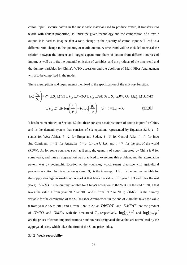
These assumptions and requirements then lead to the specification of the unit cost function:

( )13.36,,2,1,loglog

93log

776

543217

⋯=

−

+⋅+

⋅+⋅+⋅+⋅+⋅+=

iforp

pb

p

pbT

DMFATDWTOTDMFADWTODS

S

iii

iiiiiii

β

βββββα

It has been mentioned in Section 1.2 that there are seven major sources of cotton import for China,

and in the demand system that consists of six equations represented by Equation 3.13, 1=i

stands for West Africa, 2=i for Egypt and Sudan, 3=i for Central Asia, 4=i for Indo

Sub-Continent, 5=i for Australia, 6=i for the U.S.A. and 7=i for the rest of the world

(ROW). As for some countries such as Benin, the quantity of cotton imported by China is 0 for

some years, and thus an aggregation was practiced to overcome this problem, and the aggregation

pattern was by geographic location of the countries, which seems plausible with agricultural

products as cotton. In this equation system, iα is the intercept; 93D is the dummy variable for

the supply shortage in world cotton market that takes the value 1 for year 1993 and 0 for the rest

years; DWTO is the dummy variable for China’s accession to the WTO in the end of 2001 that

takes the value 1 from year 2002 to 2011 and 0 from 1992 to 2001; DMFA is the dummy

variable for the elimination of the Multi-Fiber Arrangement in the end of 2004 that takes the value

0 from year 2005 to 2011 and 1 from 1992 to 2004; DWTOT and DMFAT are the product

of DWTO and DMFA with the time trend T , respectively. ( )ppilog and ( )pp7log

are the prices of cotton imported from various sources designated above that are normalized by the

aggregated price, which takes the form of the Stone price index.

3.4.2 Weak separability

25

To explore the separability in China’s cotton import demand, three separable structures will be

introduced to the demand system, and these structures will be tested. The performance and the

influence on the model of the separable structures will be reported and discussed in the following

chapters of the thesis.

The first structure separates the cotton from different sources of import into three subsets. The

cotton from West Africa and Egypt and Sudan will be put in the same subset, which stands for the

cotton imported from Africa; the cotton from Central Asia and Indo Sub-Continent will be placed

in the same subset, thus the cotton from Asia; the cotton from Australia, the U.S.A. and the ROW

will be set together in one subset, which is the cotton from other cotton import source. Hence, the

cost function of this separable structure is:

( ) ( ) ( )( ) ( )14.3,,,,,, 7653432211 pppcppcppccc =

The restrictions for this separable structure then are 7654321 ,, bbbbbbb ==== .

The second structure separates in the following manner: the cotton from West Africa and Egypt

and Sudan in a subset Africa, the cotton from Central Asia, Indo Sub-Continent and the U.S.A. in

a subset Asia and the U.S.A., the cotton from Australia and the ROW in a subset other sources.

Accordingly, the cost function of this separable structure is:

( ) ( ) ( )( ) ( )15.3,,,,,, 7536432211 ppcpppcppccc =

The restrictions for this structure are 7564321 ,, bbbbbbb ====

The third structure has the following three subsets: the cotton from West Africa, Egypt and Sudan

and the U.S.A., thus Africa and the U.S.A., the cotton from Central Asia and Indo Sub-Continent

in a subset as Asia, the cotton from Australia and the ROW in a subset as other sources. Thus, the

following cost function holds with this separable structure:

( ) ( ) ( )( ) ( )16.3,,,,,, 7534326211 ppcppcpppccc =

The restrictions for this separable structure are 7543621 ,, bbbbbbb ==== .

26

CHAPTER 4 – ECONOMETRIC APPROACH

In this chapter, the methodology in this thesis is stated. Firstly, the basic concepts of Bayesian

econometrics will be introduced; secondly, the BBMR algorithm will be presented; finally, the

estimation methodology will be described in the context of China’s import demand system for

cotton.

4.1 A brief introduction to Bayesian econometrics

In this section, a brief outline of Bayesian econometrics will be provided with respect to the

development and application of the method, as well as its difference with the traditional

frequentist econometrics.

4.1.1 Bayes Theorem

The foundation of Bayesian econometrics as a recently developed econometric branch could be

traced back to much earlier to the famous Bayes Theorem. The theorem was named after the

English mathematician Thomas Bayes, who formulated a specific case of what was to become one

of the most widely used theorem in mathematical statistics, the Bayes Theorem. Though Bayes

himself never published the study, his work was edited by Richard Price, whose paper was

published posthumously. Finally, the current form of the theorem was further consummated and

published in 1812 by the French mathematician Pierre-Simon marquis de Laplace in his Théorie

analytique des probabilités. The modern form of the Bayes Theorem is as follows:

( ) ( ) ( )( ) ( )1.4

PrPr|Pr

|PrB

AABBA =

In Equation 4.1, ( )BA |Pr is the probability of event A taking place conditional on event B ,

and similarly is ( )AB |Pr defined. ( )APr and ( )BPr are respectively the unconditional

probabilities with which event A and B occur. In the theorem, ( )APr is called the prior

probability, or prior, and ( )BA |Pr is referred to as the posterior probability, or posterior. This

theorem is the foundation of Bayesian econometrics.

4.1.2 The Bayesian econometrics in comparison to frequentist econometrics

Bayesian econometrics is relatively new in econometric analysis and is rapidly becoming popular

in economic research. Prior to the 1970s, Bayesian methods were not very widely applied in

economics studies mainly because of the restriction in computing complexity with the approach.

27

However, with the significant growth in computer capabilities, economists have attached

increasing attention to Bayesian methods. Zellner (1971) authored the first comprehensive book

introducing Bayesian methods, and the textbook of Koop (2003) provided a more modern view on

Bayesian econometrics.

The most fundamental feature that distinguishes Bayesian econometrics to frequentist

econometrics is that in the latter, parameters are deemed fixed values and the estimators of them

are random, whilst in the former, parameters themselves are considered to be random. Thus, with

Bayesian methods, the estimation is not on the value of the parameters, but rather their posterior

distribution, combining the prior information with the information contained in the data in the

form of the likelihood function. In Bayesian econometrics, Bayesian Theorem takes another form

(Koop, 2003)

( ) ( ) ( )( ) ( )2.4

PrPr|Pr

|Pry

yy

θθθ =

In Equation 4.2, θ is the matrix of parameters and y is the vector of data that is to be

explicated by the parameters. Thus, ( )y|Pr θ , the posterior distribution of the parameters is then

the probability that they take certain values conditional on the data that is observed. ( )θ|Pr y ,

known as the likelihood function, depicts how the data observed is “generated”. The prior

information, ( )θPr , is what is already known or believed by the researchers before the data is

obtained. As ( )yPr is constant once the data is given, Equation 4.2 could be abbreviated as

indicating that the posterior distribution is proportional to the product of the likelihood and prior.

( ) ( ) ( ) ( )3.4Pr|Pr|Pr θθθ yy ∝

Here ∝ stands for “proportional to”.

With the posterior distribution of the parameters, ( )yE i |θ , the posterior mean and ( )yi |varθ ,

the posterior variance of iθ , a parameter in θ could be derived with the following formulation:

( ) ( ) ( )4.4|Pr| ∫= θθθθ dyyE iii

( ) ( ) ( ) ( ) ( )( ) ( )5.4|Pr|Pr|||var2222

∫∫ −=−= θθθθθθθθθ dydyyEyEy iiiiiii

The advantages of Bayesian methods are multifold. The one that is the most significant for this

28

study is that with frequentist econometrics, only the information contained by data is explored and

explicated; on the contrary with Bayesian methods, the believes held by the researchers out of

experiences or economic theories could be integrated into the estimation of the parameters’

posterior distribution by the inclusion of prior information. Chalfant et al. (1991) imposed

concavity and monotonicity restrictions on the expenditure functions of consumers taking an

inequality form with prior information to estimate the Canadian meat demand system with the

AIDS model. Montgomery and Rossi (1999) estimated price elasticities in a demand system with

multiple brands and stores applying the prior information derived from the additive utility

functions by hierarchical Bayesian methods, the results from simulation and real datasets revealing

that the performance with this approach outstripped that of other Bayesian and non-Bayesian

estimation. This advantage will feature as an important one in this study, the reason of which is to

be further explained in the upcoming section.

4.2 Bayesian bootstrap multivariate regression (BBMR)

The specific technique that will be used in this thesis is Bayesian bootstrap multivariate regression

(BBMR) introduced by Heckelei and Mittelhammer (2003). This section is devoted to introduce

this algorithm.

4.2.1 The development of BBMR

Bootstrap is a technique to generate sampling distribution of parameters, which was first

introduced by Efron (1979). It was natural that the Bayesian analogue was then developed, known

as the Bayesian bootstrap, which applies bootstrap technique to the former Monte Carlo

integration (MCI) that is also widely used in researches with Bayesian methods. Kloek and Dijk

(1978) used Monte Carlo to draw the posterior distributions of parameters, aiming at solving the

Bayesian methods’ unpleasant characters of in medium sample size. Zellner et al. (1988)

developed the MCI algorithm for models with potential endogeneity and consequently

identification problems to obtain the posterior distribution of reduced form and structural

parameters.

Bayesian bootstrap (BB) was introduced by Rubin (1981). BB could serve to overcome the

difficulties that Bayesian methods encounter when applied to a relatively small sample with a

complex or unfamiliar population distribution as the original sample is bootstrapped to generate a

bootstrap sample, and posterior distributions are allocated to bootstrap sample.

29

However, as pointed out by Heckelei and Mittelhammer (2003), the kernel of the posterior

allocation procedure was generated by ordered random values from a uniform distribution from 0

to 1. Accordingly, it is the inherent feature of the BB method that its posterior distribution is

tightly connected with the Dirichlet distribution, impeding its application to parameterized

equation systems. In the contrast, BBMR method bootstraps the likelihood function without the

necessity to determine the form and specification of the likelihood function itself; it fits a wider

range of choices in prior information, which could be derived from experience or theories and

provides a more general approach to estimate highly parameterized multi-equation systems with

Bayesian methods that is robust regarding the likelihood function.

4.2.2 The BBMR algorithm

As the equation system in this thesis is going to encounter endogeneity, the algorithm developed

by Heckelei et al. (1997) and Heckelei and Mittelhammer (2003) will be introduced here in this

section. Suppose that the equation system to be regressed is the following:

( )6.411 mnmkknmllnmnmn UZXY ×××××××× +++= γβαι

In Equation 4.6, Y is the matrix of n observations on each of the dependent variables in the

equation system; ι is a vector of n ones; X is the matrix of n observations on l exogenous

explanatory variables; Z is the matrix of n observations on l endogenous explanatory variables;

α , β and γ are the matrices of coefficients corresponding to the explanatory variables; U

is matrix of error terms in the structural form.

The reduced form on the endogenous variables in Equation 4.6 is like the following:

( )7.4knkppnkn VTZ ×××× += δ

In Equation 4.7, T is a matrix of exogenous variables and δ is the matrix of corresponding

reduced form coefficients. V is the reduced form error term, and its rows are independently

distributed with mean vectors of zeroes, and a covariance matrix Σ that is positive definite. Let

the posterior distribution of δ be ( )Z|Pr δ and then it will be mapped to the posterior of α ,

β and γ with the following algorithm:

1. Regress the reduced form with OLS to obtain ^

δ , the estimator of δ and the estimated

reduced form residual matrix ^

V with the following:

30

( ) ( )8.4,''^^

1^

δδ TZVZTTT −== −

And then define:

( )9.4'^^

VVS =

2. Generate N bootstrap samples of the rows in the matrix of estimated reduced for residuals:

nVVV^

2

^

1

^

,,, ⋯ to obtain N matrices NiVi ,,2,1,*⋯= . Afterwards, these matrices are

corrected with the following adjustment:

( ) NiSSSSVV iii ,,2,1,211*21***

⋯== −−

( ) ( )10.4''' 1*** TTTTIMandMVVSWith iii−−==

I in Equation 4.10 is identical matrix with the appropriate order and the exponent 1/2 is the

symmetric square root of matrices defined as SSS =2121

3. Obtain N bootstrap samples Nii ,,2,1,*⋯=δ by combining the regression structure

likelihood ),|,(^

SL δδ Σ and an ignorance prior for Σ :

( ) ( )11.4,,2,1,'' **1^

* NiVTTT ii ⋯=−= −δδ

4. With the N bootstrap samples, Nii ,,2,1,*⋯=δ , N bootstrap samples

NiZi ,,2,1,*⋯= could be obtained for Z , the matrix of endogenous variables in the

structural form:

( )12.4,,2,1,** NiTZ ii ⋯== δ

5. Insert NiZi ,,2,1,*⋯= into Equation 4.6, and estimating the structural form with two

Stage Least Square (2SLS) or three Stage Least Square (3SLS) will lead to N samples from

the posterior distribution of α , β and γ corresponding to the estimation strategy.

4.2.3 Posterior expectations and variance of the coefficients

Designate the posterior distribution of α , β and γ obtained with the algorithm above

( )Y|Pr α , ( )Y|Pr β and ( )Y|Pr γ , respectively. These posteriors are based on ignorance

priors for the coefficients that are proportional to a constant. However, in most demand systems,

31

the priors are based on inequalities regarding the coefficients to satisfy the restrictions such as the

concavity of the cost function. With this type of priors, the samples from the posteriors that satisfy

the restrictions will be assigned a prior probability of 1, and those not will be assigned to a prior

probability of 0. Hence, the posterior mean and variance are simply the sample mean and variance

of the samples of the coefficients that satisfy the restrictions.

4.3 BBMR applied to China’s cotton import demand system

4.3.1 Estimation of the model

Concerning the cotton import demand system specified in Section 3.3, the equation system

consists of six equations, whose structural form is the following:

( )13.36,,2,1,loglog

93log

776

543217

⋯=

−

+⋅+

⋅+⋅+⋅+⋅+⋅+=

iforp

pb

p

pbT

DMFATDWTOTDMFADWTODS

S

iii

iiiiiii

β

βββββα

Projecting to the designation in Equation 4.6, ( ) 6,,2,1,log 7 ⋯=iforSSi are the

dependent variables; TDMFATDWTOTDMFADWTOD ,,,,,93 and ( ),log ip

7,,2,1 ⋯=ifor are the exogenous variables in X ; ( )plog is the endogenous variable in

Z . The reduced form of the equation system in Equation 3.13 takes ( )plog as dependent

variables, and the T in Equation 4.7 includes the constant in ι and all the exogenous variables

in X . Thus there are 14 variables in T .

Similar to Heckelei et al. (1997) who studied the Japanese meat demand, the estimation strategy

adopted in this thesis is to carry out the step 5 in algorithm introduced in Section 4.2.2 is the

iterative version of the 3SLS introduced by Zellner and Theil (1962), which estimates all the

equations in a system with endogeneity simultaneously, instead of separately as the mechanism of

the 2SLS. As in this demand system the ROW was taken as the numeraire, to ensure that the

estimators of the parameters are independent on the choice of numeraire, the variance-covariance

matrix of the regression residuals of the 3SLS will be iterated until it is identical.

The BBMR algorithm for China’s demand for cotton import and relative statistical analysis are

programmed in the TSP software, and the code of the program is available in Appendix D.

4.3.2 Testing separable structures with Bayesian methods

32

Similar to frequentist econometrics, Bayesian methods also allows hypotheses to be tested.

However, as stated before, Bayesian econometrics view the parameters themselves as random

variables instead of a fixed value, and thus the hypotheses taking the form as functions of the

parameters can be directly tested with their posterior distributions. An increasingly interested and

applied approach in hypothesis testing in Bayesian methods is the Highest Posterior Density (HPD)

Intervals (HPDI). The HPDI (Koop, 2003, pp44) appears similar to the confidence interval in the

frequentist econometrics, but the similarity is only in the outlook, and these two definitions have

very different inherent thoughts behind the appearance, most obviously because the HPDI uses the

parameters, or functions of the parameters themselves to test the hypotheses.

To define the HPDI, one must first define the credible sets. Let nℜ∈θ be a vector of

parameters, and ( )θϕ f= a vector of functions of θ defined on a region Ψ with a

dimension of s with ns ≤ . If Ψ⊆Ξ is a region, and it is a α ( 1≤α ) credible set if:

( ) ( ) ( )13.4|Pr|Pr ∫Ξ ==Ξ∈ αϕϕϕ dyy

Then the α HPDI is simply the shortest α credible set. If the values of the hypotheses

functions are within the interval, then the hypotheses are maintained.

Within the context of this thesis, the test is carried out on the separable structures. All the three

separable structures have a 4-dimensional hypotheses to be tested, among which three are

common cross the structures, which take the form of 021 =− bb , 043 =− bb and 075 =− bb ,

and the particular ones with the three structures are: 076 =− bb for the first separable structure,

063 =− bb for the second separable structure and 061 =− bb for the third separable structure.

Thus, the HPDI for each separable structure are presented by two 4 by 1 vectors with the lower

and higher bound of the HPDI for each hypothesis listed above, respectively.

It is worth mentioning that the test can be imposed with another direction. As Heckelei et al. (1997)

pointed out, the smallest HPD Probability is more consistent with the Bayesian idea to test

hypotheses based on the posterior distribution of parameters and functions on them, taking a full

collection of information into account, instead on only reporting the interval that the hypotheses

are held with a preset significant level. Hence, this approach will report the smallest mass

probabilities that the function values in the hypotheses being tested are still included in the HPD

region. This approach resembles the P-value in frequentist econometrics, and the smaller the

33

smallest HPD probability, the more confirmative the data are to the hypotheses with the ignorance

prior indicated by the BBMR algorithm. To be more specific in the context of testing the separable

structures, it involves calculating the probabilities that zero are contained in the HPD of the six

hypotheses functions above to be tested.

34

CHAPTER 5 – DATA

In this chapter, the data used in this thesis will be introduced. Necessary processing has been

applied to the data to satisfy this study and they will be described in this chapter. In the meanwhile,

preliminary statistical analyses are performed and the results of it will be reported in this chapter.

The statistics are referred to Appendix B including the mean, standard error, maximum, minimum,

skewness and kurtosis of the values, quantities, prices and expenditure shares of all the sources of

import.

5.1 The source and content of the data

The data used in this thesis are provided by Food and Agriculture Organization of the United

Nations (FAO), which is one of the most authorized data sources in agricultural sector. This

dataset includes data in the quantity and value of China’s cotton imports from the entire world and

six specified regions, namely West Africa, Egypt and Sudan, Central Asia, Indo Sub-Continent,

Australia and the U.S.A, covering a time period from 1992 to 2011. The quantity in the dataset is

presented in tons, and the value of import in thousand dollars. This dataset is balanced and

includes no missing data

5.2 Processing of the data

The first step taken is to calculate the value and quantity of cotton imported by China from the

regions of origin except for the six main regions listed in Section 5.1. Combined, it is designated

the ROW for 7=i , and the calculation is simply:

( )1.5,6

17

6

17 ∑∑

==

−=−=i

iTi

iT QQQVVV

In Equation 5.1, 7V and 7Q are respectively the value and quantity of cotton imported from the

ROW; TV and TQ are respectively the total value and quantity of China’s cotton import; iV

and iQ for 6,,2,1 ⋯=i are respectively the value and quantity of cotton imported from the six

main sources of import.

As stated in Section 3.3, the price of the cotton produced in each and every region in dollar per ton

is included in the equations, and they are obtained with the following equation:

( )2.57,,2,1,1000 ⋯=×= iforQVap iii

35

In Equation 5.2, iap are the absolute prices of the import cotton, and then they are normalized to

( )tpi , the relative prices with respect to those in 2000, i.e. ( ) 12000 =ip .

( ) ( ) ( ) ( )3.520111992;7,,2,1,2000 totiforaptaptp iii === ⋯

Finally, with ( )7log SSi for 6,,2,1 ⋯=i being the dependent variables in the equation

system, iS for 7,,2,1 ⋯=i , the expenditure share of cotton import from the seven sources,

also needs to be gained with the following formula:

( )4.57,,2,1, ⋯== iforVVS Tii

5.3 Preliminary statistical analysis of the data

A glimpse at the data reveals that both the values and quantities imported from different sources

vary drastically throughout the time period. The prices and expenditure shares of the cotton import

derived from the available data also fluctuated within an extraordinarily wide range. The statistical

analyses carried out on the data are presented in the following sections

5.3.1 West Africa

The value and quantity of cotton import from West Africa was very variable. Regarding the values

of import, the maximum is more than 535 times more than the minimum, with the standard error

of the import values even larger than the mean. Similar phenomena were also observed for the

quantities. The changes in value were mainly attributed to that in the quantities of import, as the

changes in the prices of cotton imported from West Africa was not as fluctuating as the others’,

whose maximum was only 2.5 times of the minimum. The expenditure share of West African

cotton varied from 0.7% to more than 16%. Its share was generally small from 1994 to 2001, and

the minimum was observed in 2000; the share increased afterwards, reaching the maximum in

2002, but afterwards the share decreased again till 2011.

5.3.2 Egypt and Sudan

The cotton imported from Egypt and Sudan witnessed a value difference of more than 470 times

between the maximum and minimum; the maximum quantity was more than 580 times higher than

the minimum. In the meantime, the price of cotton from Egypt and Sudan also changed in a rather

large range, with the highest price reaching more than six times higher to the lowest. The

expenditure share of the cotton imported from this source was relatively small through the whole

36

time period with a minimum of less than 0.3% and even the maximum share was lower than 6%.

5.3.3 Central Asia

The more than 530 times difference in values of cotton imported from Central Asia was mainly

contributed by the changes in prices. The flux in quantities of import from this region was

relatively small compared to the other sources of import, with the maximum 157 times more than

the minimum. In contrast, the prices changed dramatically during the 20 years of interest, as the

maximum price was more than 9.6 times higher than the minimum. As for the expenditure share of

Central Asian cotton, the maximum was around 18%, whilst the minimum was a little more than

0.7%; the share increased through the 90s till the millennium, and then it decreased in trend till

2011.

5.3.4 Indo Sub-Continent

The values of cotton import from Indo Sub-Continent fluctuated the most dramatically during the

two decades in this thesis, with the maximum value more than 6300 times higher than the

minimum. The quantities of import from this region also varied tremendously, as the peak quantity

almost 780 times as large as the lowest one. Both the highest value and quantity of import took

place in 2011. Indian cotton’s price saw a difference of more than 8 times during the two decades.

The cotton imported from this region accounted for a highly varied share of China’s total cotton

import expenditure. Its share was relatively low before 2005 with the minimum just above 0.2%

while the share grew greatly since 2006 and saw the highest of more than 31%. This increase is

partly related to the introduction of Bt cotton in cotton sectors in Indo Sub-Continent.

5.3.5 Australia

Australia exports more than 90% of its cotton output. China importing values of cotton from

Australia have undergone a 640 times difference between the maximum and minimum from 1992

to 2011. The maximum quantity of cotton imported from this source was almost 300 times greater

than the minimum. The prices were less variable than the others’, as the highest price was less

than 2.5 times higher than the lowest. The share of Australian cotton started with a minimum of

less than 1.5% in 1992, and increased in trend during the 90s till 2001 with the maximum of 24%

in 1999; then it went through a decrease in recent years with a share of around 5% while it

increased again to more than 16% in 2011.

37

5.3.6 The U.S.A.

The United States has long been the biggest cotton exporter to China. The import value of U.S.

cotton was the second most fluctuating in the period only after Indo Sub-Continent with the

maximum more than 1490 times more than the minimum. The import quantities from the U.S.A.

also experienced great difference with the largest quantity more than 450 times greater than the

minimum. Regarding the price, U.S. cotton had a highest price more than 5.5 times the lowest. As

the biggest cotton import source of China, the U.S.A. accounted for up to more than 64% of the

total cotton import expenditure of China, while the lowest share of just below 8% took place in

1993, the year that saw a major supply shortage. Except for 1993, the U.S. cotton never took a

smaller share than 25%, with a mean of more than 45%. However, there was a trend in recent

years as in 2011 the U.S. cotton had a share of 30% in China’s cotton import.

5.3.7 The rest of world (ROW)

As the combination of all the cotton import sources other than the six major ones introduced above,

the ROW had a maximum value of cotton imported by China 140 times higher than the minimum,

which is the smallest change in value among all the sources. The quantities of the cotton import

from the ROW were also the least variable among the sources, which differed 17 times between

the largest and smallest. On the contrary to the values and quantities of cotton import from the

ROW, its prices was the most variable with the highest price more than 13 times higher than the

lowest one. The expenditure share of cotton from the ROW was the lowest in 2008, which was a

little more than 6%, while the highest share was in 1993 with the shortage of supply in the six

major import sources, which was above 46%. Except for the extreme share in 1993, the

expenditure shares of the ROW were relatively stable, which were divided into two periods:

before 2000, it was between 10% and 22%, and afterwards, it reduced to between 6% and 10%

with the exception for 2011 when the share was more than 13%. The ROW was chosen in the

empirical model as the numeraire, though the choice of it should not influence the result as the

iterative 3SLS was used to estimate the demand system with the Bayesian bootstrapped

endogenous variables, which has been explicated in Section 4.3.

5.4 Conclusion

From the preliminary statistical analyses on the original and derivative data, it can be concluded

that the values, quantities, prices and expenditure shares of all the sources varied significantly

38

throughout the whole time period. All sources of import witnessed a variant of more than 400

times in the values of import with the exception of the ROW; and the import quantities of them

also experienced a dramatic fluctuation in the quantities of import. The overall cotton import of

China increased with a great scale after its accession to the WTO, and accorded the international

economic situation as stated in Section 1.2. The prices of China’s cotton import from different

sources also witnessed a tremendous flux, which had a similar trend in which the prices first

decreased gradually before around year 2000, and then increased rapidly in recent years. After the

processing performed on the data, they can serve to analyze the demand system of China’s cotton

import.

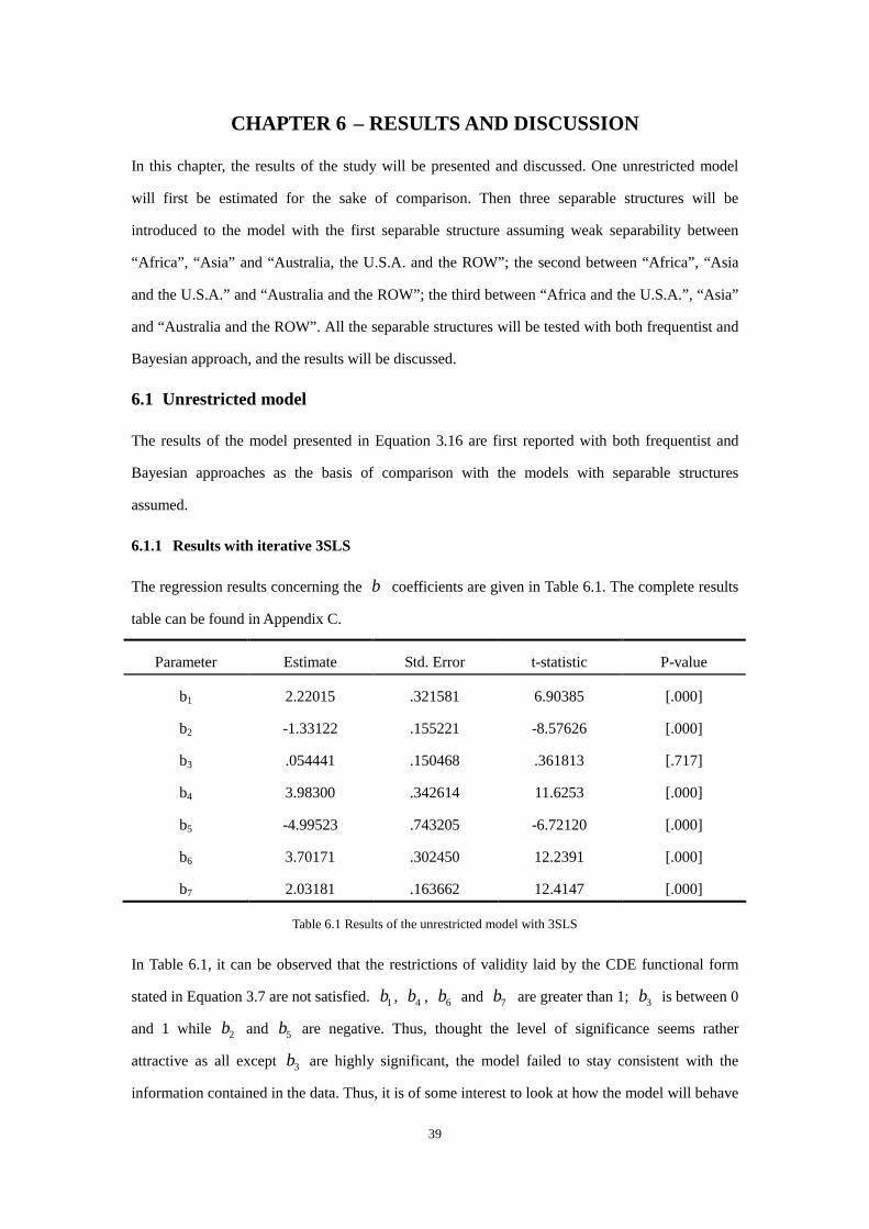
39

CHAPTER 6 – RESULTS AND DISCUSSION

In this chapter, the results of the study will be presented and discussed. One unrestricted model

will first be estimated for the sake of comparison. Then three separable structures will be

introduced to the model with the first separable structure assuming weak separability between

“Africa”, “Asia” and “Australia, the U.S.A. and the ROW”; the second between “Africa”, “Asia

and the U.S.A.” and “Australia and the ROW”; the third between “Africa and the U.S.A.”, “Asia”

and “Australia and the ROW”. All the separable structures will be tested with both frequentist and

Bayesian approach, and the results will be discussed.

6.1 Unrestricted model

The results of the model presented in Equation 3.16 are first reported with both frequentist and

Bayesian approaches as the basis of comparison with the models with separable structures

assumed.

6.1.1 Results with iterative 3SLS

The regression results concerning the b coefficients are given in Table 6.1. The complete results

table can be found in Appendix C.

Parameter Estimate Std. Error t-statistic P-value

b1 2.22015 .321581 6.90385 [.000]

b2 -1.33122 .155221 -8.57626 [.000]

b3 .054441 .150468 .361813 [.717]

b4 3.98300 .342614 11.6253 [.000]

b5 -4.99523 .743205 -6.72120 [.000]

b6 3.70171 .302450 12.2391 [.000]

b7 2.03181 .163662 12.4147 [.000]

Table 6.1 Results of the unrestricted model with 3SLS

In Table 6.1, it can be observed that the restrictions of validity laid by the CDE functional form

stated in Equation 3.7 are not satisfied. 1b , 4b , 6b and 7b are greater than 1; 3b is between 0

and 1 while 2b and 5b are negative. Thus, thought the level of significance seems rather

attractive as all except 3b are highly significant, the model failed to stay consistent with the

information contained in the data. Thus, it is of some interest to look at how the model will behave

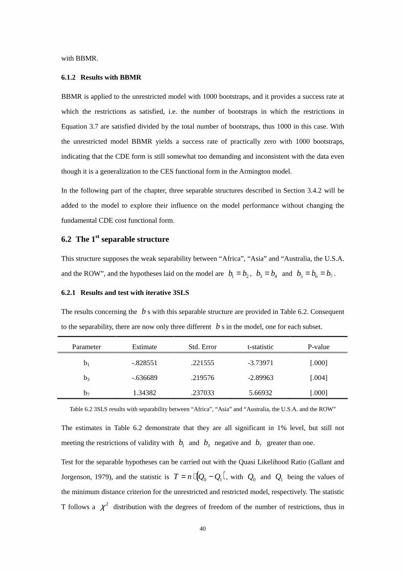
40

with BBMR.

6.1.2 Results with BBMR

BBMR is applied to the unrestricted model with 1000 bootstraps, and it provides a success rate at

which the restrictions as satisfied, i.e. the number of bootstraps in which the restrictions in

Equation 3.7 are satisfied divided by the total number of bootstraps, thus 1000 in this case. With

the unrestricted model BBMR yields a success rate of practically zero with 1000 bootstraps,

indicating that the CDE form is still somewhat too demanding and inconsistent with the data even

though it is a generalization to the CES functional form in the Armington model.

In the following part of the chapter, three separable structures described in Section 3.4.2 will be

added to the model to explore their influence on the model performance without changing the

fundamental CDE cost functional form.

6.2 The 1st separable structure

This structure supposes the weak separability between “Africa”, “Asia” and “Australia, the U.S.A.

and the ROW”, and the hypotheses laid on the model are 21 bb = , 43 bb = and 765 bbb == .

6.2.1 Results and test with iterative 3SLS

The results concerning the b s with this separable structure are provided in Table 6.2. Consequent

to the separability, there are now only three different b s in the model, one for each subset.


b1 -.828551 .221555 -3.73971 [.000]

b3 -.636689 .219576 -2.89963 [.004]

b7 1.34382 .237033 5.66932 [.000]

Table 6.2 3SLS results with separability between “Africa”, “Asia” and “Australia, the U.S.A. and the ROW”

The estimates in Table 6.2 demonstrate that they are all significant in 1% level, but still not

meeting the restrictions of validity with 1b and 3b negative and 7b greater than one.

Test for the separable hypotheses can be carried out with the Quasi Likelihood Ratio (Gallant and

Jorgenson, 1979), and the statistic is ( )10 QQnT −⋅= , with 0Q and 1Q being the values of

the minimum distance criterion for the unrestricted and restricted model, respectively. The statistic

T follows a 2χ distribution with the degrees of freedom of the number of restrictions, thus in

41

this case a 2χ distribution with four degrees of freedom. The result of the test is in Table 6.3

0Qn ⋅ 1Qn ⋅ T P-value ( 24χ )

67.8713 56.7148 11.1565 .0248603

Table 6.3 QLR test for the separability between “Africa”, “Asia” and “Australia, the U.S.A. and the ROW”

As shown in Table 6.3, the statistic has a P-value of 0.025. This separable structure does not seem

very plausible with frequentist econometric test, as the hypothesis of the hypotheses laid on the

model according to the separable structure can be rejected in the 5% level of significance.

6.2.2 Results and test with BBMR

The BBMR with this separable structure leads to a success rate, i.e. the probability of the

restrictions being satisfied of 22.4%, indicating an improvement regarding the consistency of the

model with the data compared with the unrestricted model without any weak separability among

the cotton import sources assumed. The results of the BBMR are reported below in Table 6.4

including the posterior means and standard errors of the b s, as well as the minimum and

maximum value within the bootstraps where the restrictions are satisfied.

Parameter Posterior Mean Posterior S.D. Min Max

b1 0.24216 0.15092 0.00067083 0.65765

b3 0.53014 0.25587 0.012523 0.99099

b7 0.45514 0.24910 0.012216 0.99669

Success Rate 22.4%

Table 6.4 BBMR results with separability between “Africa”, “Asia” and “Australia, the U.S.A. and the ROW”

The posterior distribution of the own-price Allen elasticities of substitution (AES) can then be

calculated with Equation 3.12, and they are reported below in Table 6.5.

Own-price AES Posterior Mean Posterior S.D. Min Max

σ11 -8.56949 1.52519 -11.03462 -4.11650

σ22 -33.24628 6.43713 -43.45481 -15.26419

σ33 -3.98569 1.79418 -7.71165 -0.73031

σ44 -3.89582 1.74530 -7.52283 -0.72859

σ55 -5.27118 2.27470 -9.32428 -0.29843

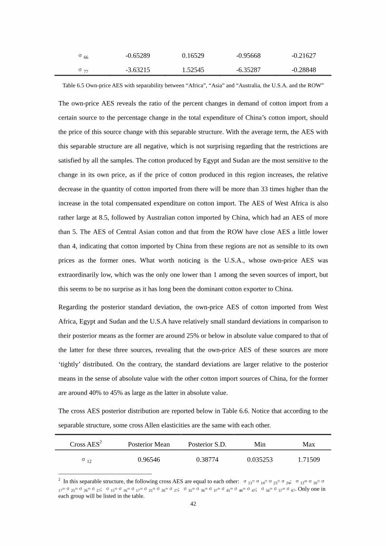
42

σ66 -0.65289 0.16529 -0.95668 -0.21627

σ77 -3.63215 1.52545 -6.35287 -0.28848

Table 6.5 Own-price AES with separability between “Africa”, “Asia” and “Australia, the U.S.A. and the ROW”

The own-price AES reveals the ratio of the percent changes in demand of cotton import from a

certain source to the percentage change in the total expenditure of China’s cotton import, should

the price of this source change with this separable structure. With the average term, the AES with

this separable structure are all negative, which is not surprising regarding that the restrictions are

satisfied by all the samples. The cotton produced by Egypt and Sudan are the most sensitive to the

change in its own price, as if the price of cotton produced in this region increases, the relative

decrease in the quantity of cotton imported from there will be more than 33 times higher than the

increase in the total compensated expenditure on cotton import. The AES of West Africa is also

rather large at 8.5, followed by Australian cotton imported by China, which had an AES of more

than 5. The AES of Central Asian cotton and that from the ROW have close AES a little lower

than 4, indicating that cotton imported by China from these regions are not as sensible to its own

prices as the former ones. What worth noticing is the U.S.A., whose own-price AES was

extraordinarily low, which was the only one lower than 1 among the seven sources of import, but

this seems to be no surprise as it has long been the dominant cotton exporter to China.

Regarding the posterior standard deviation, the own-price AES of cotton imported from West

Africa, Egypt and Sudan and the U.S.A have relatively small standard deviations in comparison to

their posterior means as the former are around 25% or below in absolute value compared to that of

the latter for these three sources, revealing that the own-price AES of these sources are more

‘tightly’ distributed. On the contrary, the standard deviations are larger relative to the posterior

means in the sense of absolute value with the other cotton import sources of China, for the former

are around 40% to 45% as large as the latter in absolute value.

The cross AES posterior distribution are reported below in Table 6.6. Notice that according to the

separable structure, some cross Allen elasticities are the same with each other.

Cross AES2 Posterior Mean Posterior S.D. Min Max

σ12 0.96546 0.38774 0.035253 1.71509

2 In this separable structure, the following cross AES are equal to each other: σ13=σ14=σ23=σ24; σ13=σ16=σ

17=σ25=σ26=σ27; σ15=σ16=σ17=σ25=σ26=σ27; σ35=σ36=σ37=σ45=σ46=σ47; σ56=σ57=σ67. Only one in each group will be listed in the table.

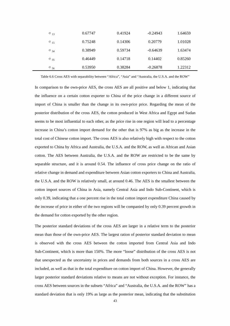
43

σ13 0.67747 0.41924 -0.24943 1.64659

σ15 0.75248 0.14306 0.20779 1.01028

σ34 0.38949 0.59734 -0.64639 1.63474

σ35 0.46449 0.14718 0.14402 0.85260

σ56 0.53950 0.38284 -0.26878 1.22312

Table 6.6 Cross AES with separability between “Africa”, “Asia” and “Australia, the U.S.A. and the ROW”

In comparison to the own-price AES, the cross AES are all positive and below 1, indicating that

the influence on a certain cotton exporter to China of the price change in a different source of

import of China is smaller than the change in its own-price price. Regarding the mean of the

posterior distribution of the cross AES, the cotton produced in West Africa and Egypt and Sudan

seems to be most influential to each other, as the price rise in one region will lead to a percentage

increase in China’s cotton import demand for the other that is 97% as big as the increase in the

total cost of Chinese cotton import. The cross AES is also relatively high with respect to the cotton

exported to China by Africa and Australia, the U.S.A. and the ROW, as well as African and Asian

cotton. The AES between Australia, the U.S.A. and the ROW are restricted to be the same by

separable structure, and it is around 0.54. The influence of cross price change on the ratio of

relative change in demand and expenditure between Asian cotton exporters to China and Australia,

the U.S.A. and the ROW is relatively small, at around 0.46. The AES is the smallest between the

cotton import sources of China in Asia, namely Central Asia and Indo Sub-Continent, which is

only 0.39, indicating that a one percent rise in the total cotton import expenditure China caused by

the increase of price in either of the two regions will be companied by only 0.39 percent growth in

the demand for cotton exported by the other region.

The posterior standard deviations of the cross AES are larger in a relative term to the posterior

mean than those of the own-price AES. The largest ration of posterior standard deviation to mean

is observed with the cross AES between the cotton imported from Central Asia and Indo

Sub-Continent, which is more than 150%. The more “loose” distribution of the cross AES is not

that unexpected as the uncertainty in prices and demands from both sources in a cross AES are

included, as well as that in the total expenditure on cotton import of China. However, the generally

larger posterior standard deviations relative to means are not without exception. For instance, the

cross AES between sources in the subsets “Africa” and “Australia, the U.S.A. and the ROW” has a

standard deviation that is only 19% as large as the posterior mean, indicating that the substitution

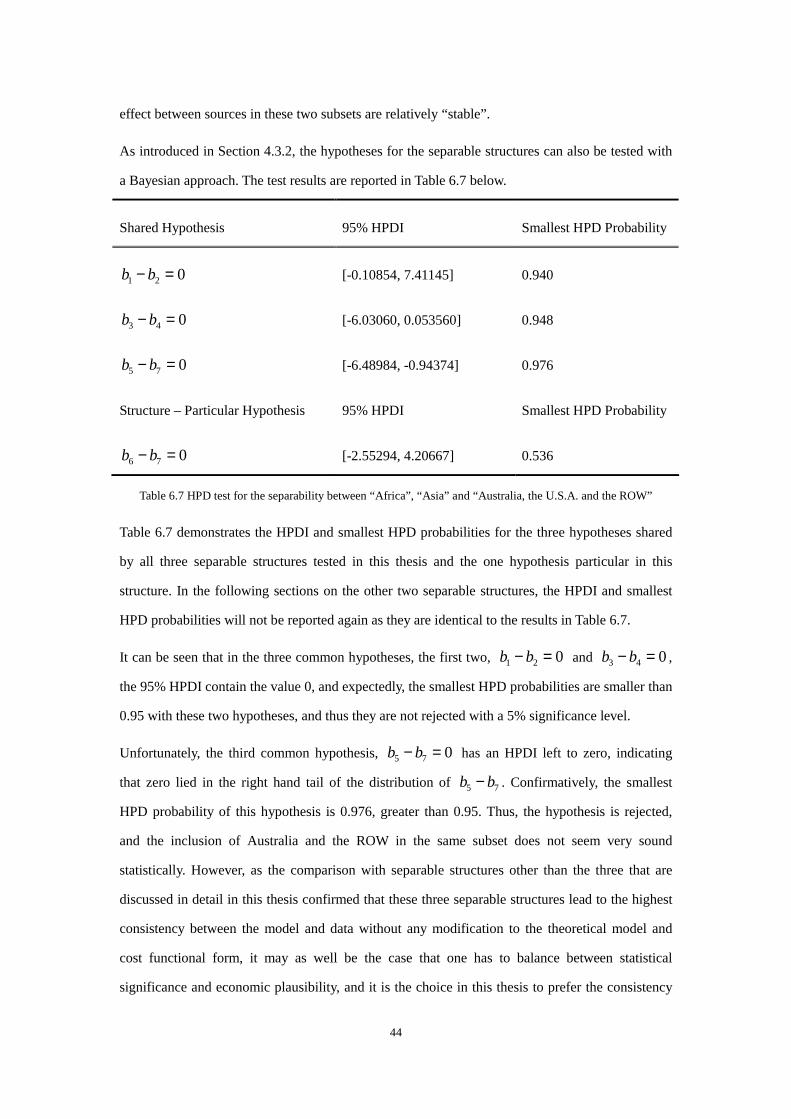
44

effect between sources in these two subsets are relatively “stable”.

As introduced in Section 4.3.2, the hypotheses for the separable structures can also be tested with

a Bayesian approach. The test results are reported in Table 6.7 below.

Shared Hypothesis 95% HPDI Smallest HPD Probability

021 =− bb [-0.10854, 7.41145] 0.940

043 =− bb [-6.03060, 0.053560] 0.948

075 =− bb [-6.48984, -0.94374] 0.976

Structure – Particular Hypothesis 95% HPDI Smallest HPD Probability

076 =− bb [-2.55294, 4.20667] 0.536

Table 6.7 HPD test for the separability between “Africa”, “Asia” and “Australia, the U.S.A. and the ROW”

Table 6.7 demonstrates the HPDI and smallest HPD probabilities for the three hypotheses shared

by all three separable structures tested in this thesis and the one hypothesis particular in this

structure. In the following sections on the other two separable structures, the HPDI and smallest

HPD probabilities will not be reported again as they are identical to the results in Table 6.7.

It can be seen that in the three common hypotheses, the first two, 021 =− bb and 043 =− bb ,

the 95% HPDI contain the value 0, and expectedly, the smallest HPD probabilities are smaller than

0.95 with these two hypotheses, and thus they are not rejected with a 5% significance level.

Unfortunately, the third common hypothesis, 075 =− bb has an HPDI left to zero, indicating

that zero lied in the right hand tail of the distribution of 75 bb − . Confirmatively, the smallest

HPD probability of this hypothesis is 0.976, greater than 0.95. Thus, the hypothesis is rejected,

and the inclusion of Australia and the ROW in the same subset does not seem very sound

statistically. However, as the comparison with separable structures other than the three that are

discussed in detail in this thesis confirmed that these three separable structures lead to the highest

consistency between the model and data without any modification to the theoretical model and

cost functional form, it may as well be the case that one has to balance between statistical

significance and economic plausibility, and it is the choice in this thesis to prefer the consistency

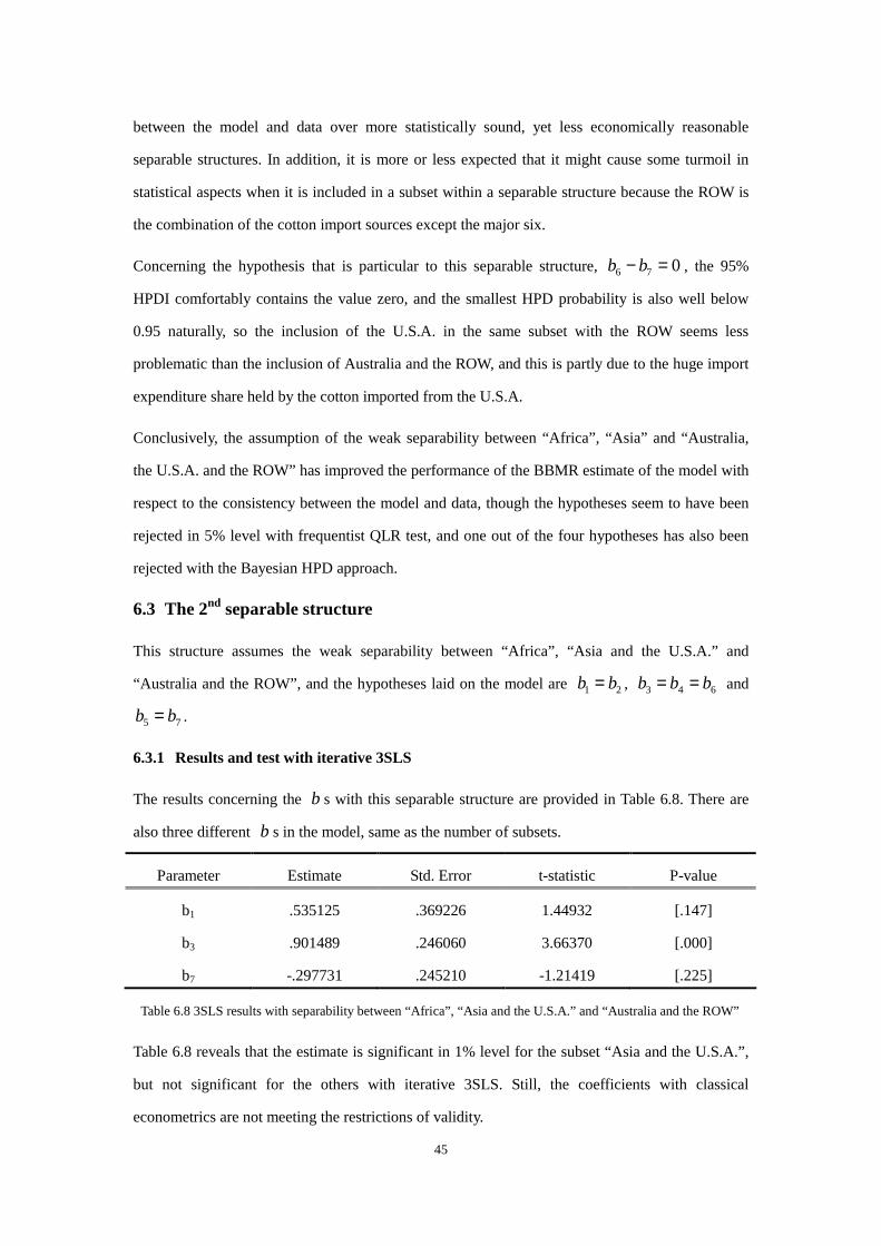
45

between the model and data over more statistically sound, yet less economically reasonable

separable structures. In addition, it is more or less expected that it might cause some turmoil in

statistical aspects when it is included in a subset within a separable structure because the ROW is

the combination of the cotton import sources except the major six.

Concerning the hypothesis that is particular to this separable structure, 076 =− bb , the 95%

HPDI comfortably contains the value zero, and the smallest HPD probability is also well below

0.95 naturally, so the inclusion of the U.S.A. in the same subset with the ROW seems less

problematic than the inclusion of Australia and the ROW, and this is partly due to the huge import

expenditure share held by the cotton imported from the U.S.A.

Conclusively, the assumption of the weak separability between “Africa”, “Asia” and “Australia,

the U.S.A. and the ROW” has improved the performance of the BBMR estimate of the model with

respect to the consistency between the model and data, though the hypotheses seem to have been

rejected in 5% level with frequentist QLR test, and one out of the four hypotheses has also been

rejected with the Bayesian HPD approach.

6.3 The 2nd separable structure

This structure assumes the weak separability between “Africa”, “Asia and the U.S.A.” and

“Australia and the ROW”, and the hypotheses laid on the model are 21 bb = , 643 bbb == and

75 bb = .


The results concerning the b s with this separable structure are provided in Table 6.8. There are

also three different b s in the model, same as the number of subsets.


b1 .535125 .369226 1.44932 [.147]

b3 .901489 .246060 3.66370 [.000]

b7 -.297731 .245210 -1.21419 [.225]

Table 6.8 3SLS results with separability between “Africa”, “Asia and the U.S.A.” and “Australia and the ROW”

Table 6.8 reveals that the estimate is significant in 1% level for the subset “Asia and the U.S.A.”,

but not significant for the others with iterative 3SLS. Still, the coefficients with classical

econometrics are not meeting the restrictions of validity.

46

Test for separability with the Quasi Likelihood Ratio is reported in Table 6.9.


67.8713 58.8731 8.9982 . 0611445

Table 6.9 QLR test for the separability between “Africa”, “Asia and the U.S.A.” and “Australia and the ROW”

This separable structure appears to be more plausible than the first one, as the hypothesis of the

restriction can not be rejected in the 5% level of significance, but rejected in 10% significance

level. Thus the plausibility of this separable structure is somewhat ambiguous with the frequentist

econometrics approach.


The BBMR with this separable structure leads to a success rate of 39.4%. The results taking the

form of posterior means and standard errors, as well as the minimum and maximum value within

the bootstraps where the restrictions are satisfied are reported here in Table 6.10.


b1 0.29476 0.17688 0.00016773 0.85024

b3 0.74349 0.13224 0.16912 0.99614

b7 0.29781 0.16870 0.0044466 0.93932

Success Rate 39.4%

Table 6.10 BBMR results for the separability between “Africa”, “Asia and the U.S.A.” and “Australia and the ROW”

The performance of BBMR with this separable structure has improved considerably in comparison

to that of the first one with respect to the success rate. It seems that the aggregation of this

structure is more consistent to the information contained in the data.

With the bootstrap outcome above, the own-price Allen elasticities of substitution (AES) are

reported below in Table 6.11


σ11 -7.86476 1.86576 -11.03292 -1.90113

σ22 -30.82870 7.62410 -43.58931 -6.77768

σ33 -2.27765 1.04378 -6.76458 -0.28019

47

σ44 -2.22859 1.01849 -6.60565 -0.27945

σ55 -6.48624 1.45176 -9.04898 -0.99892

σ66 -0.45045 0.10337 -0.88257 -0.21304

σ77 -4.37393 0.94541 -6.08577 -0.81640

Table 6.11 Own-price AES with the separability between “Africa”, “Asia and the U.S.A.” and “Australia and ROW”

The outline of own-price AES in this separable structure is similar to the one with the first

separable structure. The most elasticities of substitution in this structure have a smaller posterior

mean in absolute value with the exception of the own-price AES of the cotton imported from

Australia and the ROW. The largest own-price AES is that of the cotton imported from Egypt and

Sudan with a value of -30.8 indicating that the price rise of the cotton imported by China from this

region leading to a expenditure rise of one percent will cause a decrease of more than 30% in the

cotton import demand from this region. This result is consistent with the last separable structure. A

likely reason for this phenomenon is that the cotton imported from this region accounted for a

relatively small share in the Chinese cotton demand, as stated in Section 5.3.2; accompanied by

the drastically fluctuating price of the it, it is understandable that the cotton from Egypt and Sudan

has an extremely high AES.

Just as the situation of the first separable structure, the smallest own-price AES is also observed

with the U.S.A., the increase in the price of the U.S. cotton will lead to only 0.45 times as large a

decrease in China’s cotton demand for it as an increase in the total compensated expenditure on

cotton import of China. Consistent with the first separable structure, this could be explicated with

the huge share of the U.S. cotton in China’s cotton import. As Vlontzos and Duquenne (2007)

claimed, even without an official agreement between China and the U.S.A., the Chinese cotton

import market is somehow dominated by the U.S. cotton for a long period. As stated in Section

5.3.6, the U.S. cotton witnessed peak share of more than 60% in the total value of cotton import of

China, and its share remained remarkably high even though its price has been fluctuating in a

rather large range. This led to the result that the price changes will lead to a great change in

China’s cotton import expenditure as the U.S. cotton accounted for such a large percentage in it,

yet the demand for the U.S. cotton is not that sensitive to price regarding the data.

The own-price AES of the other sources of import are also close to those with the first separable

structure. They are all negative and above one in absolute value, suggesting that if the prices of

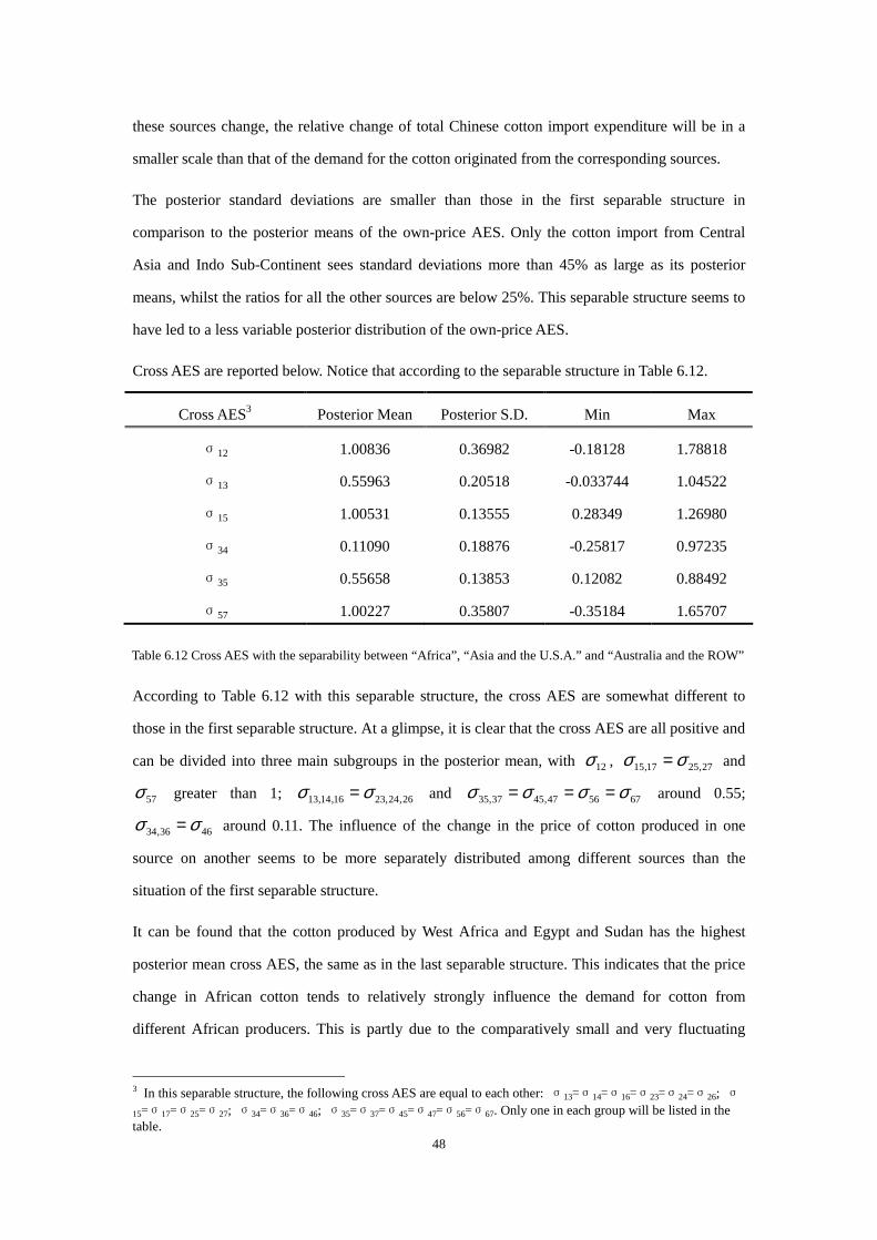
48

these sources change, the relative change of total Chinese cotton import expenditure will be in a

smaller scale than that of the demand for the cotton originated from the corresponding sources.

The posterior standard deviations are smaller than those in the first separable structure in

comparison to the posterior means of the own-price AES. Only the cotton import from Central

Asia and Indo Sub-Continent sees standard deviations more than 45% as large as its posterior

means, whilst the ratios for all the other sources are below 25%. This separable structure seems to

have led to a less variable posterior distribution of the own-price AES.

Cross AES are reported below. Notice that according to the separable structure in Table 6.12.


σ12 1.00836 0.36982 -0.18128 1.78818

σ13 0.55963 0.20518 -0.033744 1.04522

σ15 1.00531 0.13555 0.28349 1.26980

σ34 0.11090 0.18876 -0.25817 0.97235

σ35 0.55658 0.13853 0.12082 0.88492

σ57 1.00227 0.35807 -0.35184 1.65707

Table 6.12 Cross AES with the separability between “Africa”, “Asia and the U.S.A.” and “Australia and the ROW”

According to Table 6.12 with this separable structure, the cross AES are somewhat different to

those in the first separable structure. At a glimpse, it is clear that the cross AES are all positive and

can be divided into three main subgroups in the posterior mean, with 12σ , 27,2517,15 σσ = and

57σ greater than 1; 26,24,2316,14,13 σσ = and 675647,4537,35 σσσσ === around 0.55;

4636,34 σσ = around 0.11. The influence of the change in the price of cotton produced in one

source on another seems to be more separately distributed among different sources than the

situation of the first separable structure.

It can be found that the cotton produced by West Africa and Egypt and Sudan has the highest

posterior mean cross AES, the same as in the last separable structure. This indicates that the price

change in African cotton tends to relatively strongly influence the demand for cotton from

different African producers. This is partly due to the comparatively small and very fluctuating

3 In this separable structure, the following cross AES are equal to each other: σ13=σ14=σ16=σ23=σ24=σ26; σ

15=σ17=σ25=σ27; σ34=σ36=σ46; σ35=σ37=σ45=σ47=σ56=σ67. Only one in each group will be listed in the table.

49

share in expenditure of cotton from this region, as well as fairly strong substitution effect between

the cotton produced by African exporters, leading to the fact that the changes in price of one

African import source will cause somewhat strong influence on the demand for cotton from

another African country, and impact the total expenditure on cotton import of China with the same

direction but slightly smaller in relative scale. Similar conclusions could be drawn on the subset

“Africa” and “Australia and the ROW” with the second highest cross AES, as well as Australia

and the ROW with a cross AES above 1 under this separability assumption, where the situation

resembles the former case.

The posterior mean of cross AES between the subset “Africa” and “Asia and the U.S.A.”, along

with that between subsets “Asia and the U.S.A.” and “Australia and the ROW” are both around

0.55. This implies that the substitution effect between these two pairs are not as strong as the three

discussed in the last paragraph. The potential reason for the phenomena could be two-fold. On the

one hand, the price change in one subset in the two pairs has relatively small influence on the

demand for cotton imported from the other in the same pairs. On the other hand, the impact laid by

the price change on one another in either of the two pairs is further diluted by the prevailing

expenditure share held by the subset “Asia and the U.S.A.” leading to great percentage variance in

total cotton import expenditure should the price change.

Within the subset “Asia and the U.S.A.”, the lowest posterior mean of cross AES is observed with

this separable structure. At 0.11, it is lower than the posterior mean of the AES within the subset

“Asia” in the first separable structure, which was also the lowest in that separable structure. This

could be explained in the same manner with the case of cross AES between “Africa” and “Asia

and the U.S.A.” and that between “Asia and the U.S.A.” and “Australia and the ROW”. The

inclusion of the U.S.A. seems to have laid similar impact on the AES.

Similar to the situation of own-price AES, the posterior standard deviations in comparison to the

posterior means of the cross AES also is smaller than in the first separable structure. One

noteworthy point is the ratio between posterior standard deviation and mean still well higher than

150% in the cross AES between Central Asia, Indo Sub-Continent and the U.S.A., which are in the

same subset in this separable structure. It seems that the substitution effect between these sources

has become even more variable with the inclusion of the U.S.A. in the subset.

Similarly, the separability between “Africa”, “Asia and the U.S.A.” and “Australia and the ROW”

50

is tested with the Bayesian approach. Only the results of the constraints particular in this separable

structure are reported in Table 6.13.


063 =− bb [-7.09208, 1.54325] 0.878

Table 6.13 HPD test for the separability between “Africa”, “Asia and the U.S.A.” and “Australia and the ROW”

From Table 6.13, it can be seen that the 95% HPDI for this particular hypothesis contains the

value 0, and accordingly, smallest HPD probability is below 0.95. Thus, the hypothesis that

063 =− bb is not rejected, and it seems plausible to include the U.S. cotton in the same subset as

the Asian cotton.

To conclude, the second separable structure, which is the weak separability between “Africa”,

“Asia and the U.S.A.” and “Australia and the ROW” is more plausible than the first separable

structure discussed in Section 6.2, for it is not rejected in 5% level (still rejected in 10% level), and

the particular hypothesis in the structure is also maintained with Bayesian methods. Besides, it

provides a considerably higher success rate, implying an improvement in consistency with

compared to the first separable structure.

6.4 The 3rd separable structure

This structure assumes the weak separability between “Africa and the U.S.A.”, “Asia” and

“Australia and the ROW”, and the hypotheses laid on the model are 621 bbb == , 43 bb = and

75 bb = .


The results concerning the b s are reported in Table 6.14. Again, only three b s are different from

each other.


b1 .961036 .400071 2.40216 [.016]

b3 .695808 .264895 2.62673 [.009]

b7 -.451963 -.451963 -1.75765 [.079]

Table 6.14 3SLS results with separability between “Africa and the U.S.A.”, “Asia” and “Australia and the ROW”

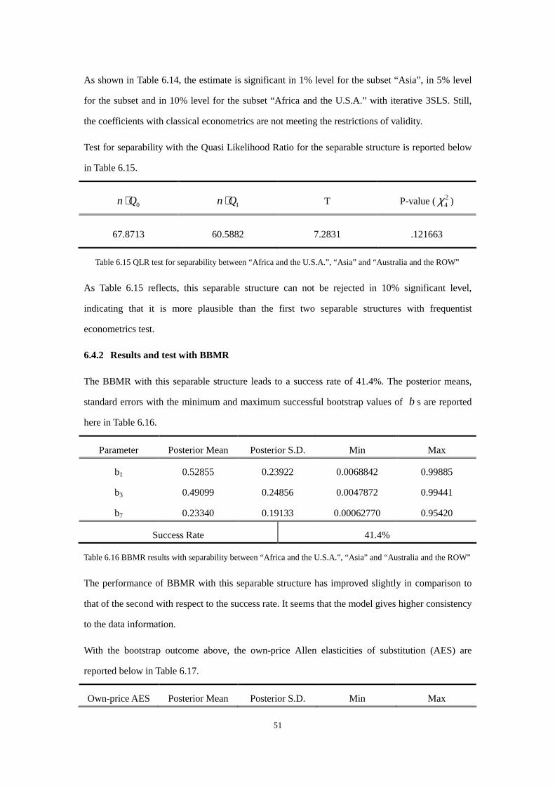
51

As shown in Table 6.14, the estimate is significant in 1% level for the subset “Asia”, in 5% level

for the subset and in 10% level for the subset “Africa and the U.S.A.” with iterative 3SLS. Still,

the coefficients with classical econometrics are not meeting the restrictions of validity.

Test for separability with the Quasi Likelihood Ratio for the separable structure is reported below

in Table 6.15.


67.8713 60.5882 7.2831 .121663

Table 6.15 QLR test for separability between “Africa and the U.S.A.”, “Asia” and “Australia and the ROW”

As Table 6.15 reflects, this separable structure can not be rejected in 10% significant level,

indicating that it is more plausible than the first two separable structures with frequentist

econometrics test.


The BBMR with this separable structure leads to a success rate of 41.4%. The posterior means,

standard errors with the minimum and maximum successful bootstrap values of b s are reported

here in Table 6.16.


b1 0.52855 0.23922 0.0068842 0.99885

b3 0.49099 0.24856 0.0047872 0.99441

b7 0.23340 0.19133 0.00062770 0.95420

Success Rate 41.4%

Table 6.16 BBMR results with separability between “Africa and the U.S.A.”, “Asia” and “Australia and the ROW”

The performance of BBMR with this separable structure has improved slightly in comparison to

that of the second with respect to the success rate. It seems that the model gives higher consistency

to the data information.

With the bootstrap outcome above, the own-price Allen elasticities of substitution (AES) are

reported below in Table 6.17.


52

σ11 -5.53458 2.61693 -11.23669 -0.39045

σ22 -20.88591 10.40643 -43.57438 -0.42778

σ33 -4.26759 1.81406 -7.89002 -0.59855

σ44 -4.17023 1.76658 -7.70072 -0.59748

σ55 -7.18799 1.58631 -9.15679 -1.08003

σ66 -0.63466 0.13318 -0.94817 -0.26430

σ77 -4.88194 1.01126 -6.15053 -0.94226

Table 6.17 Own-price AES with the separability between “Africa and the U.S.A.”, “Asia” and “Australia and ROW”

Concerning the own-price AES in this separable structure, it remains similar to those in the first

two, with all the posterior means negative and the absolute value between 4 to 10 with the

exception of Egypt and Sudan, and the U.S.A. However, in this separable structure, the posterior

mean of cotton imported from Egypt and Sudan is notably smaller in absolute value that the cased

in the first two structures. This could be the result of the fact that this region is now allocated to

the same subset with the U.S.A. unlike in the first two separable structures. On the contrary, the

own-price AES of the U.S.A. is not that much influenced with its dominant expenditure share.

Regarding the deviation, this separable structure results in ratios of the posterior standard

deviation relative to the means in absolute value that are overall higher than those produced by the

second separable structure. The own-price AES of Australia, the U.S.A. and the ROW have

posterior standard deviations less than 25% as large as posterior means, and for the other resources

the ratios are above 40%. What is interesting here is that the standard deviation of the own-price

AES of Egyptian and Sudanese cotton has increase considerably relative to its posterior mean

compared to the first two separable structures. The own-price AES of cotton from this region

seems to have become more variable with the inclusion of the U.S.A. in the same subset. Keeping

in mind that the posterior mean of the AES of the same source has also greatly decreased as the

U.S.A. was put in the same subset, it appears that the U.S. cotton has a great impact on the AES

posterior distribution of Egypt and Sudan, which is consistent with the conclusion of Pan et al.

(2005b).However, the influence is not observed in the opposite direction, as the U.S. cotton

own-price AES still appears with a low ratio between the posterior standard deviation and

posterior mean, not different from the situations in the first two separable structures.

Cross AES with this separable structure are reported below in Table 6.18.

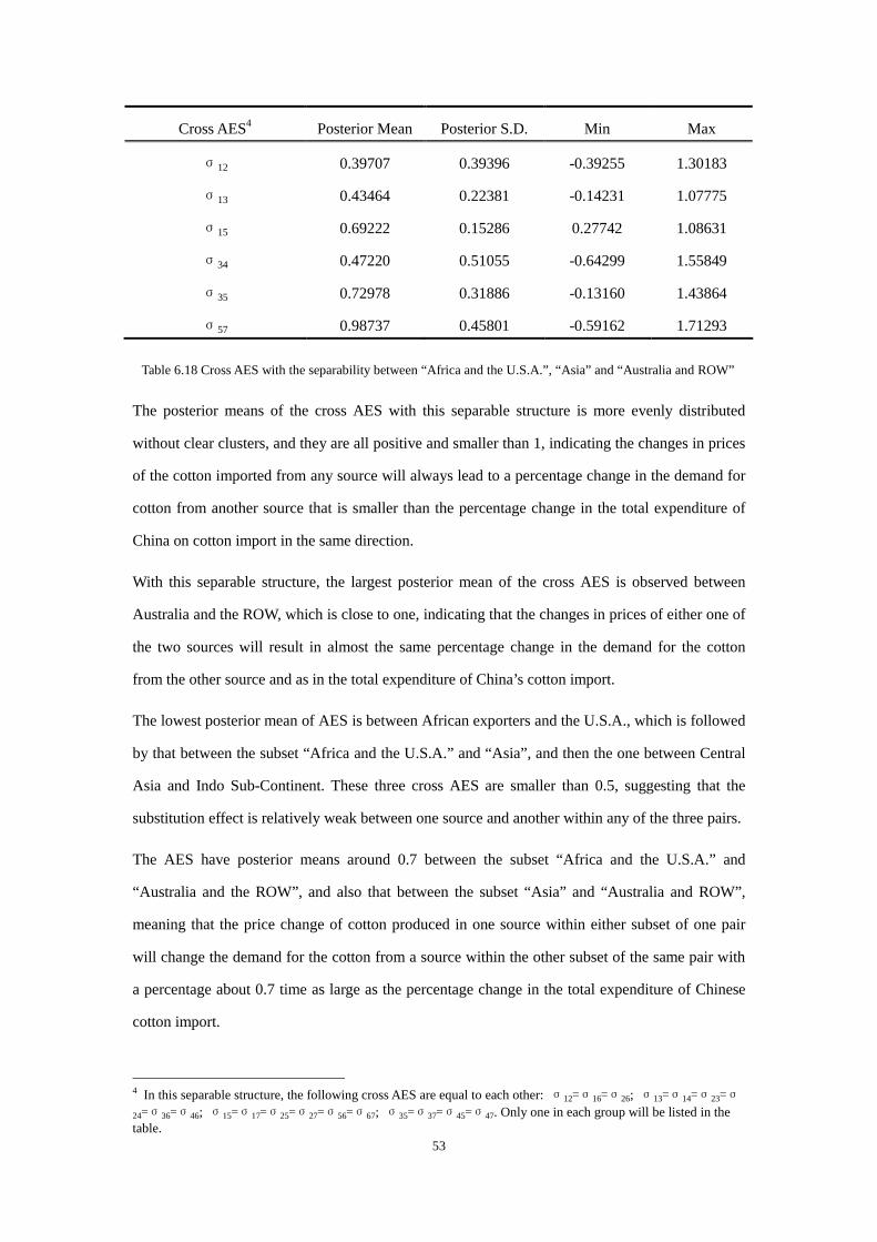
53


σ12 0.39707 0.39396 -0.39255 1.30183

σ13 0.43464 0.22381 -0.14231 1.07775

σ15 0.69222 0.15286 0.27742 1.08631

σ34 0.47220 0.51055 -0.64299 1.55849

σ35 0.72978 0.31886 -0.13160 1.43864

σ57 0.98737 0.45801 -0.59162 1.71293

Table 6.18 Cross AES with the separability between “Africa and the U.S.A.”, “Asia” and “Australia and ROW”

The posterior means of the cross AES with this separable structure is more evenly distributed

without clear clusters, and they are all positive and smaller than 1, indicating the changes in prices

of the cotton imported from any source will always lead to a percentage change in the demand for

cotton from another source that is smaller than the percentage change in the total expenditure of

China on cotton import in the same direction.

With this separable structure, the largest posterior mean of the cross AES is observed between

Australia and the ROW, which is close to one, indicating that the changes in prices of either one of

the two sources will result in almost the same percentage change in the demand for the cotton

from the other source and as in the total expenditure of China’s cotton import.

The lowest posterior mean of AES is between African exporters and the U.S.A., which is followed

by that between the subset “Africa and the U.S.A.” and “Asia”, and then the one between Central

Asia and Indo Sub-Continent. These three cross AES are smaller than 0.5, suggesting that the

substitution effect is relatively weak between one source and another within any of the three pairs.

The AES have posterior means around 0.7 between the subset “Africa and the U.S.A.” and

“Australia and the ROW”, and also that between the subset “Asia” and “Australia and ROW”,

meaning that the price change of cotton produced in one source within either subset of one pair

will change the demand for the cotton from a source within the other subset of the same pair with

a percentage about 0.7 time as large as the percentage change in the total expenditure of Chinese

cotton import.

4 In this separable structure, the following cross AES are equal to each other: σ12=σ16=σ26; σ13=σ14=σ23=σ

24=σ36=σ46; σ15=σ17=σ25=σ27=σ56=σ67; σ35=σ37=σ45=σ47. Only one in each group will be listed in the table.

54

The cross AES posterior standard deviation has similar behavior with that in the first separable

structure. The posterior standard deviations of the cross AES are larger in the relative sense to the

posterior means compared to the case in own-price AES. Once again, the ratio of the cross AES

posterior standard deviation to posterior mean between the cotton imported from Central Asia and

Indo Sub-Continent is the largest and higher than one, further confirming the conclusion with the

first two separable structures.

Test results for the particular constraint in this separable structure are presented in Table 6.19.


061 =− bb [-2.80300, 2.58693] 0.082

Table 6.19 HPD test for the separability between “Africa and the U.S.A.”, “Asia” and “Australia and the ROW”

Table 6.19 demonstrates that the particular hypothesis in this separable structure has a 95% HPDI

containing zero and the smallest HPD probability is the lowest among the six constraints in total at

0.082. Thus, this constraint is not rejected, and the separable structure seems more plausible than

the first two with Bayesian HPD test, similar to the conclusion drawn from the frequentist

econometrics test.

6.5 Conclusion

As the iterative 3SLS estimates of the substitution coefficients fail to satisfy the restrictions,

BBMR and three separable structures are deployed to estimate the posterior distribution of the

coefficients, leading to the posterior of own-price and cross AES. The posterior distributions are

somewhat similar among the own-price AES posterior mean, and the behavior of Egypt and Sudan,

and the U.S.A. are especially worth noticing, as the former has the largest posterior mean in

absolute value; the latter is the smallest, and the only own-price AES posterior mean smaller than

1 in absolute value with all three separable structures. Yet the posterior standard deviations seem

to be more impacted by different separable structures. This is especially remarkable with whether

to include the U.S.A. in the same subset with Egypt and Sudan. The U.S.A. appears to be very

influential concerning the own-price AES posterior standard deviation in a relative sense to the

own-price AES posterior mean of the cotton from this source of import.

Concerning the cross AES, the posterior distributions are more dependent on different separable

55

structures. With the first and third separable structures, all the posterior means of AES are between

0 and 1, whilst with the second, they appear in three clusters, one slightly above 1, one around

0.55 and the other about 0.11. The behavior of posterior standard deviations of the cross AES also

varies among the three separable structures analyzed in this chapter. With the first and the third

separable structures, the posterior standard deviations of the cross AES appear to be rather large in

comparison to the posterior means, yet it was relatively small in the second separable structure.

However, there is an obvious shared feature with the cross AES posterior standard deviation,

namely that the cross AES between Central Asia and Indo Sub-Continent appear to be very

variable as its posterior standard deviations are larger than its posterior means in all three

separable structures.

The three separable structures have different plausibility. The first structure can be rejected in 5%

level; the second can be rejected in 10% level but not in 5%; the third one cannot be rejected in

10% level and appears to be the most plausible one. Tests have also been carried out on the three

separable structures with Bayesian HPD as well. It seems that the inclusion of Australia and the

ROW in the same subset is not accepted, yet this might be a price one must pay to set the model in

a more economically plausible manner. Other hypotheses laid on the model by the separable

structures are accepted by the Bayesian HPD test. The extent to which the model is consistent to

the data is reflected by the success rate in Bayesian bootstrap. The first separable structure leads to

a success rate of 22.4%; the second structure results in a success rate of 39.4%, which is much

better than the first one; the third structure obtained a success rate of 41.4%, slightly improved

compared with the second one. In comparison, the Armington Model with the CES functional

form results in a success rate of almost 100%, yet this is in the cost of sacrificing the possibility to

test any separability among different sources of import, and is simply one more compromise one

must make.

56

CHAPTER 7 – CONCLUSION

China is the biggest producer of cotton and the biggest importer as well because of the huge textile

production and exporting industry. In the year 2011 China imported more than 3.5 million tons of

cotton from seven main sources of import around the world, namely West Africa, Egypt and Sudan,

Central Asia, Indo Sub-Continent, Australia, the U.S.A. and the Rest of the World. With such a

large market, it is worth investigating China’s cotton import demand system, especially the

substitution effects between different sources of import.

The Armington Model is often used in trade of agricultural products by differentiating the

products by the geographic regions of production, but the limits of the Armington Model are many,

among which is the same constant substitution between commodities from all regions caused by

the CES functional form it used in underlying the cost (or utility) function. Another major problem

of the Armington Model is the exclusion of the possibility to test separability among different

products. These can be remedied by introducing a Constant Difference of Elasticity functional

form in the cost (or utility) functions, leading to a generalization of the Armington Model.

To study the cotton import structure of China, a two-stage procedure similar to the Armington

Model was set and the CDE functional form was employed to generalize the Armington Model. As

cotton is mostly used as intermediate product to produce textiles, it is a two-stage cost

minimization procedure. In the first stage, the textile industry of China is considered to be

minimizing its total cost by deciding the quantities of different inputs. Then in the second stage,

the Chinese Government, which has been controlling the cotton import of the country, closes the

gap between domestic cotton production and the total cotton demand by imported cotton, and in

the meantime, minimizes the total import cost on cotton by allocating the total expenditure on the

cotton imported from various sources with linear homogeneity.

As the iterative 3SLS estimators failed to satisfy the restrictions laid by the CDE functional form,

the BBMR is hired to estimate the model in a Bayesian approach, investigating the posterior

distribution of the coefficients and Allen elasticities of substitution among different sources of

import, with the restrictions of the CDE functional form as the prior information. A success rate, in

other words, the probability of the restrictions being satisfied in bootstraps was reported as a sign

of consistency between the model and data.

As the success rate of bootstraps with the unrestricted model was practically zero, the hint was that

57

the CDE functional form may still be too restrictive with its implicit additivity, and a more flexible

functional form may be more consistent with the data. However, to test the goodness of fit of the

model to the data information without changing the fundamental CDE functional form, three weak

separable structures were introduced to the model, and were tested with both frequentist and

Bayesian approaches. With the frequentist QLR test, the separability among “Africa”, “Asia” and

“Australia, the U.S.A. and the ROW” was rejected in a 5% significance level; the separability

among “Africa”, “Asia and the U.S.A.” and “Australia and the ROW” was not rejected in a 5%

significance level, but was rejected in a 10% level; the separability among “Africa and the U.S.A.”,

“Asia” and “Australia and the ROW” was not rejected even in a 10% level. With the Bayesian

HPD test, all the hypotheses laid by the three separable structures were not rejected except for the

inclusion of Australia and the ROW in one subset, which unfortunately, was present in all three

separable structures. Nevertheless, this may be a compromise one must make with statistical

soundness for the sake of economic plausibility, as these three separable structures were the ones

with the highest success rates in bootstrap thus the consistency between the model and the data,

which were 22.4%, 39.4% and 41.4% in order.

With the posterior means of the own-price AES, it can be concluded that the cotton from the U.S.A

was the least sensitive to the changes in its own price, while that from Egypt and Sudan was the

most sensitive, and this conclusion held mutually with all three separable structures. The posterior

standard deviations were more impacted by different separable structures, especially remarkable

with whether to include the U.S.A. in the same subset with Egypt and Sudan. The U.S.A. appeared

to be very influential concerning the own-price AES posterior standard deviation in a relative

sense to the own-price AES posterior mean of the cotton from this source of import, while the

conclusion in a reversed direction did not hold.

For the cross AES, all the posterior means of AES are between 0 and 1 with the first and third

separable structures, whilst with the second, they appear in three clusters, yet the conclusion could

be drawn that the overall substitution effects between the cotton from different sources were

relatively small. The posterior standard deviations of the own-price AES were quite dependent on

the specification of the separable structures as they were relatively small in the second whilst

rather large with the other two. Despite of this, one may still conclude that the cross AES between

Central Asia and Indo Sub-Continent appeared to be very variable as its posterior standard

deviations were larger than its posterior means in all three separable structures.

58

REFERENCE

Articles:

1. Yearbook, C. S. (2012). National Bureau of statistics of China. China Statistical Yearbook.

2. U.S. International Trade Commission, 2011, China’s Agricultural Trade: Competitive

Conditions and Effects on U.S. Exports.

3. Hongxing, N. (2013). Agricultural Domestic Support and Sustainable Development in China.

Issue Paper No. 47. International Centre for Trade and Sustainable Development, Geneva.

4. Wakelyn, P.J. & Chaudhry, M.R. (2010). Cotton: Technology for the 21st Century.

International Cotton Advisory Committee, Washington, ISBN 9780979390357.

5. Hanoch, G. (1975). Production and demand models with direct or indirect implicit additivity.

Econometrica, 43(3): 395-419.

6. Heckelei, T. & Mittelhammer R. (2003). Bayesian bootstrap multivariate regression. Journal

of Econometrics, 112: 241-264.

7. Theil, T. (1965). The Information Approach to Demand Analysis. Econometrica, 33(1): 67-87.

8. Barten, A.P. (1966). Evidence on the Slutsky Conditions for Demand Functions. Review of

Economics and Statistics, 49: 77-84.

9. Deaton, A. & Muellbauer, J. (1980). An Almost Ideal Demand System. American Economic

Review, 70: 312-326.

10. Alston, J.M. & Chalfant, J.A. (1993). The Silence of the Lambdas: A Test of the Almost Ideal

and Rotterdam Models. American Journal of Agricultural Economics, 75(2): 304-313.

11. Sarker, R. & Surry, Y. (2006). Product differentiation and trade in agri-food products: taking

stock and looking forward. Journal of International Agricultural Trade and Development,

2(1): 39-79.

12. Armington, P.S. (1969). A theory of demand for products distinguished by place of production.

IMF Staff Papers, 16: 159-178.

13. Alston, J., Carter, C., Green, R. & Pick, D. (1990). Whither Armington trade models?

American Journal of Agricultural Economics, 72: 455-467.

14. Ito, S., Chen, D.T. & Peterson, E.W.F. (1990). Modeling international trade flows and market

shares for agricultural commodities: a modified Armington procedure for rice. Agricultural

Economics, 4: 315-333.

15. Yang, S.R. & Koo, W.W. (1993). A generalized Armington trade model: respecification.

59

Agricultural Economics, 9: 347-356.

16. Goldman, S. M., & Uzawa, H. (1964). A note on separability in demand

analysis. Econometrica, 32(3), 387-398.

17. Gorman, W. M. (1959). Separable utility and aggregation. Econometrica, 27(3), 469-481.

18. Strotz, R. H. (1959). The Utility Tree--A Correction and Further Appraisal. Econometrica,

27(3), 482-488.

19. Strotz, R. H. (1957). The empirical implications of a utility tree. Econometrica, 25(2),

269-280.

20. Pearce, I. F. (1961). An exact method of consumer demand analysis. Econometrica, 29(4),

499-516.

21. Edgerton, D. L. (1997). Weak separability and the estimation of elasticities in multistage

demand systems. American Journal of Agricultural Economics, 79(1), 62-79.

22. Christensen, L.R., Jorgenson, D.W. & Lau, L.J. (1973). Transcendental logarithmic production

frontiers. Review of Economics and Statistics, 55: 28-45.

23. Dar, A. & Dasgupta, S. (1985). The estimation of production functions: the CRES and CDE

approaches applied to US manufacturing data – a comparative study. Applied Economics, 17:

437-449.

24. Mukerji, V. (1963). Generalized SMAC Function with Constant Ratios of Elasticities of

Substitution. Review of Economic Studies, 30: 233-236.

25. Hanoch, G. (1971). CRESH production functions. Econometrica, 39(5): 695-712.

26. Surry, Y. (1993). The ‘Constant Difference of Elasticities’ function with applications to the EC

animal feed sector. Journal of Agricultural Economics, 44(1): 110-125.

27. Surry, Y., Herrard, N. & Le Roux, Y. (2002). Modeling trade in processed food products: an

econometric investigation for France. European Review of Agricultural Economics, 29(1):

1-27.

28. Baffes, J. (2004). Cotton market settings, trade policies, and issues. World Bank Policy

Research Working Paper No. WPS 3218.

29. Minot, N., & Daniels, L. (2005). Impact of global cotton markets on rural poverty in

Benin. Agricultural Economics, 33(3), 453-466.

30. Hudson, D., & Coble, K. (1999). Harvest contract price volatility for cotton. Journal of

Futures Markets, 19(6), 717-733.

60

31. Pan, S., Mohanty, S., Ethridge, D. & Fadiga, F. (2006). The Impacts of U.S. Cotton Programs

on the World Market: An Analysis of Brazilian WTO Petition. Journal of Cotton Science, 10:

180-192.

32. Pan, S., Mohanty, S., Fadiga, M., & Ethridge, D. (2004). Structural models of the United

States and the rest-of-the-world natural fiber market. Cotton Economics Research Institute

Working Paper, 04-03.

33. Pan, S., Welch, M., Mohanty, S., Fadiga, M., & Ethridge, D. (2005a). Assessing the Impacts

of the Chinese TRQ System and the US Subsidies on the World Cotton Market. The Estey

Centre Journal of International Law and Trade Policy, 6(2): 251-273.

34. Pan, S., Fadiga, M., Mohanty, S., & Welch, M. (2007). Cotton in a free trade world. Economic

Inquiry, 45(1), 188-197.

35. Fadiga, M. L., & Misra, S. K. (2007). Common trends, common cycles, and price

relationships in the international fiber market. Journal of Agricultural and Resource

Economics, 32(1), 154-168.

36. Mutuc, M. E. M., Hudson, D., & Reeves, J. M. (2012). The Effects of Uniform Climate

Change on International Cotton Prices and Production. In 2012 Conference, August 18-24,

2012, Foz do Iguacu, Brazil (No. 126362). International Association of Agricultural

Economists.

37. Lohmar, B., & Skully, D. (2003, June). China’s TRQ administration after one year: Crossing

the river by feeling for stones. In Annual Meeting of the International Agricultural Trade

Research Consortium (pp. 17-19).

38. Ge, Y., Wang, H. H., & Ahn, S. K. (2010). Cotton market integration and the impact of China's

new exchange rate regime. Agricultural Economics, 41(5), 443-451.

39. Vlontzos, G., & Duquenne, M. N. (2007, July). Evolution of trade flows for Chinese cotton.

In 2007 Summer Symposium of the International Agricultural Trade Research Consortium

(IATRC).

40. Pray, C., Ma, D., Huang, J., & Qiao, F. (2001). Impact of Bt cotton in China. World

Development, 29(5), 813-825.

41. Fang, C., & Babcock, B. A. (2003). China's cotton policy and the impact of China's WTO

accession and Bt cotton adoption on the Chinese and US cotton sectors. Center for

Agricultural and Rural Development, Iowa State University.

61

42. MacDonald, S., Pan, S., Somwaru, A., & Tuan, F. (2010). China's role in world cotton and

textile markets: a joint computable general equilibrium/partial equilibrium approach. Applied

Economics, 42(7), 875-885.

43. Yang, Y., Martin, W., & Yanagishima, K. (1997). Evaluating the benefits of abolishing the

MFA in the Uruguay Round package. Global Trade Analysis: modeling and applications,

253-79.

44. Babula, R. (1987). An Armington model of US cotton exports. Journal of Agricultural

Economics Research, 39(4), 12-22.

45. Chang, H. S. C., & Nguyen, C. (2002). Elasticity of demand for Australian cotton in

Japan. Australian Journal of Agricultural and Resource Economics, 46(1), 99-113.

46. MacDonald, S., Pan, S., Hudson, D., & Tuan, F. C. (2011). Toward a Consumer Economy in

China: Implications of Changing Wage Policies for US Cotton Exports. In 2011 Annual

Meeting, July 24-26, 2011, Pittsburgh, Pennsylvania (No. 103615). Agricultural and Applied

Economics Association.

47. Lopez, J. A., & Malaga, J. E. (2004). European Union Cotton Demand: An Application Of

Demand Systems And Panel Data. In 2004 Annual Meeting, February 14-18, 2004, Tulsa,

Oklahoma (No. 34660). Southern Agricultural Economics Association.

48. Pick, D. H., & Park, T. (1989). Export Supply and Import Demand Elasticities in the Japanese

Textile Industry: A Production Theory Approach (No. 51255). International Agricultural Trade

Research Consortium.

49. Roy, R. (1947). La distribution du revenu entre les divers biens. Econometrica, 15(3),

205-225.

50. Zellner, A. (1971). An Introduction to Bayesian Inference in Econometrics. New York: John

Wiley & Sons.

51. Moschini, G., Moro, D., & Green, R. D. (1994). Maintaining and testing separability in

demand systems. American Journal of Agricultural Economics, 76(1), 61-73.

52. Koop, G. (2003). Bayesian Econometrics. New York: John Wiley & Sons.

53. Chalfant, J. A., Gray, R. S., & White, K. J. (1991). Evaluating prior beliefs in a demand

system: the case of meat demand in Canada. American Journal of Agricultural Economics,

73(2), 476-490.

54. Montgomery, A. L., & Rossi, P. E. (1999). Estimating price elasticities with theory-based

62

priors. Journal of Marketing Research, 36(4), 413-423.

55. Efron, B. (1979). Bootstrap methods: another look at the jackknife. The annals of Statistics,

7(1), 1-26.

56. Kloek, T., & Van Dijk, H. K. (1978). Bayesian estimates of equation system parameters: an

application of integration by Monte Carlo. Econometrica, 46(1), 1-19.

57. Zellner, A., Bauwens, L., & Van Dijk, H. K. (1988). Bayesian specification analysis and

estimation of simultaneous equation models using Monte Carlo methods. Journal of

Econometrics, 38(1), 39-72.

58. Rubin, D. B. (1981). The Bayesian bootstrap. The annals of statistics, 9(1), 130-134.

59. Heckelei, T., Mittelhammer, R. C., & Wahl, T. I. (1997). Bayesian Analysis of a Japanese

Meat Demand System: A Robust Likelihood Approach (No. 18783).

60. Zellner, A., & Theil, H. (1962). Three-stage least squares: simultaneous estimation of

simultaneous equations. Econometrica, 30(1), 54-78.

61. Gallant, A. R., & Jorgenson, D. W. (1979). Statistical inference for a system of simultaneous,

non-linear, implicit equations in the context of instrumental variable estimation. Journal of

Econometrics, 11(2), 275-302.

62. Pan, S., Mohanty, S., & Fadiga, M. L. (2005b). The impacts of US cotton programs on the

west and central African countries cotton export earnings.

Websites:

1. WTO Trade Policy Review Body. (2012). WTO Trade Policy Review: China, Secretariat

Report. http://www.wto.org/english/tratop_e/tpr_e/tp364_e.htm

2. WTO Trade Policy Review Body. (2012). WTO Government Report China.

http://www.wto.org/english/tratop_e/tpr_e/tp364_e.htm

3. Food and Agriculture Organization of the United Nations.

http://www.fao.org/index_en.htm

63

APPENDIX A – FIGURES IN THE THESIS

Figure 1.1: Domestic cotton production of China from 1992 to 2011

Figure 1.2: China’s cotton import quantities from different sources

Domestic Cotton Production of China

300

400

500

600

700

800

1992

1994

1996

1998

2000

2002

2004

2006

2008

2010

Year

Qua

ntity

(10

000

tons

)

China's Cotton Import Quantities from Different Sources

0

500000

1000000

1500000

2000000

2500000

3000000

3500000

4000000

4500000

1992

1994

1996

1998

2000

2002

2004

2006

2008

2010

Year

Quantit

y (ton

)

West Africa Egypt & Sudan Central Asia Indo Subcontinent

Australia U.S.A. ROW QTOT

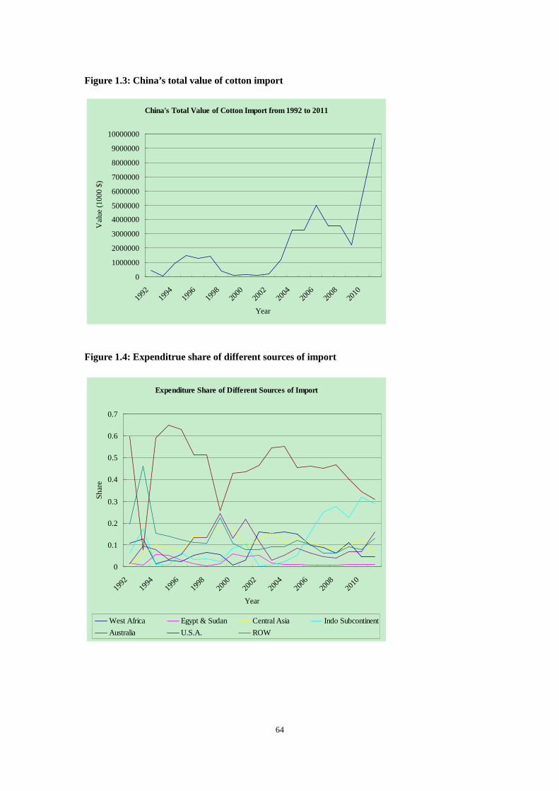
64

Figure 1.3: China’s total value of cotton import

Figure 1.4: Expenditrue share of different sources of import

China's Total Value of Cotton Import from 1992 to 2011

0

1000000

2000000

3000000

4000000

5000000

6000000

7000000

8000000

9000000

10000000

1992

1994

1996

1998

2000

2002

2004

2006

2008

2010

Year

Val

ue (

1000

$)

Expenditure Share of Different Sources of Import

0

0.1

0.2

0.3

0.4

0.5

0.6

0.7

1992

1994

1996

1998

2000

2002

2004

2006

2008

2010

Year

Sha

re

West Africa Egypt & Sudan Central Asia Indo Subcontinent

Australia U.S.A. ROW

65

APPENDIX B – PRELIMINARY STTISTICS OF THE DATA

B. 1 West Africa

West Africa Mean Std. Dev Minimum Maximum

Value (1000 $) 172689.86489 186628.37726 957.08099 512497.93750

Quantity (ton) 112606.77587 127902.20361 747.42902 390779.53125

Price (2000=1) 1.24485 0.26182 0.79834 1.99644

Share 0.079481 0.050782 0.0069759 0.16029

Table B.1 Preliminary statistics of the data of West Africa

B. 2 Egypt and Sudan

Egypt and Sudan Mean Std. Dev Minimum Maximum

Value (1000 $) 29052.79498 26224.83118 192.54100 92233.65625

Quantity (ton) 13092.11666 10541.11182 65.00700 37829.53906

Price (2000=1) 1.08464 0.36627 0.36419 2.19724

Share 0.022152 0.019427 0.0026425 0.059556

Table B.2 Preliminary statistics of the data of Egypt and Sudan

B. 3 Central Asia

Central Asia Mean Std. Dev Minimum Maximum

Value (1000 $) 216594.10484 220147.97615 1410.28699 757460.68750

Quantity (ton) 173720.88396 138680.81904 3014.02490 475324.93750

Price (2000=1) 3.60345 2.09545 1.00000 9.66899

Share 0.10739 0.042852 0.0071425 0.18117

Table B.3 Preliminary statistics of the data of Central Asia

B. 4 Indo Sub-Continent

Indo Sub-Continent Mean Std. Dev Minimum Maximum

Value (1000 $) 414642.77924 745487.33078 444.91400 2805763.50000

Quantity (ton) 242552.66621 359683.41328 1408.48096 1110873.75000

Price (2000=1) 2.86592 1.42186 0.78238 6.27569

Share 0.10964 0.10745 0.0022300 0.31837

Table B.4 Preliminary statistics of the data of Indo Sub-Continent

B. 5 Australia

Australia Mean Std. Dev Minimum Maximum

Value (1000 $) 188188.67684 340040.51381 2419.94800 1549105.62500

Quantity (ton) 95090.24604 124043.04253 1777.18701 529687.25000

Price (2000=1) 1.19513 0.28840 0.85527 2.11660

Share 0.093769 0.061561 0.014096 0.24506

66

Table B.5 Preliminary statistics of the data of Central Asia

B. 6 U.S.A.

U.S.A. Mean Std. Dev Minimum Maximum

Value (1000 $) 956823.38704 871720.85747 1998.43604 2979460.00000

Quantity (ton) 586470.17124 502868.80280 3803.28809 1747803.75000

Price (2000=1) 1.77670 0.67390 0.64917 3.62963

Share 0.45695 0.13562 0.079305 0.64863

Table B.6 Preliminary statistics of the data of the U.S.A.

B. 7 ROW

ROW Mean Std. Dev Minimum Maximum

Value (1000 $) 226708.37051 283520.20325 8886.54004 1259432.75000

Quantity (ton) 182957.23066 152008.36821 29154.55859 516330.12500

Price (2000=1) 2.95455 1.54396 0.54975 7.15700

Share 0.13061 0.088007 0.062780 0.46064

Table B.7 Preliminary statistics of the data of the ROW

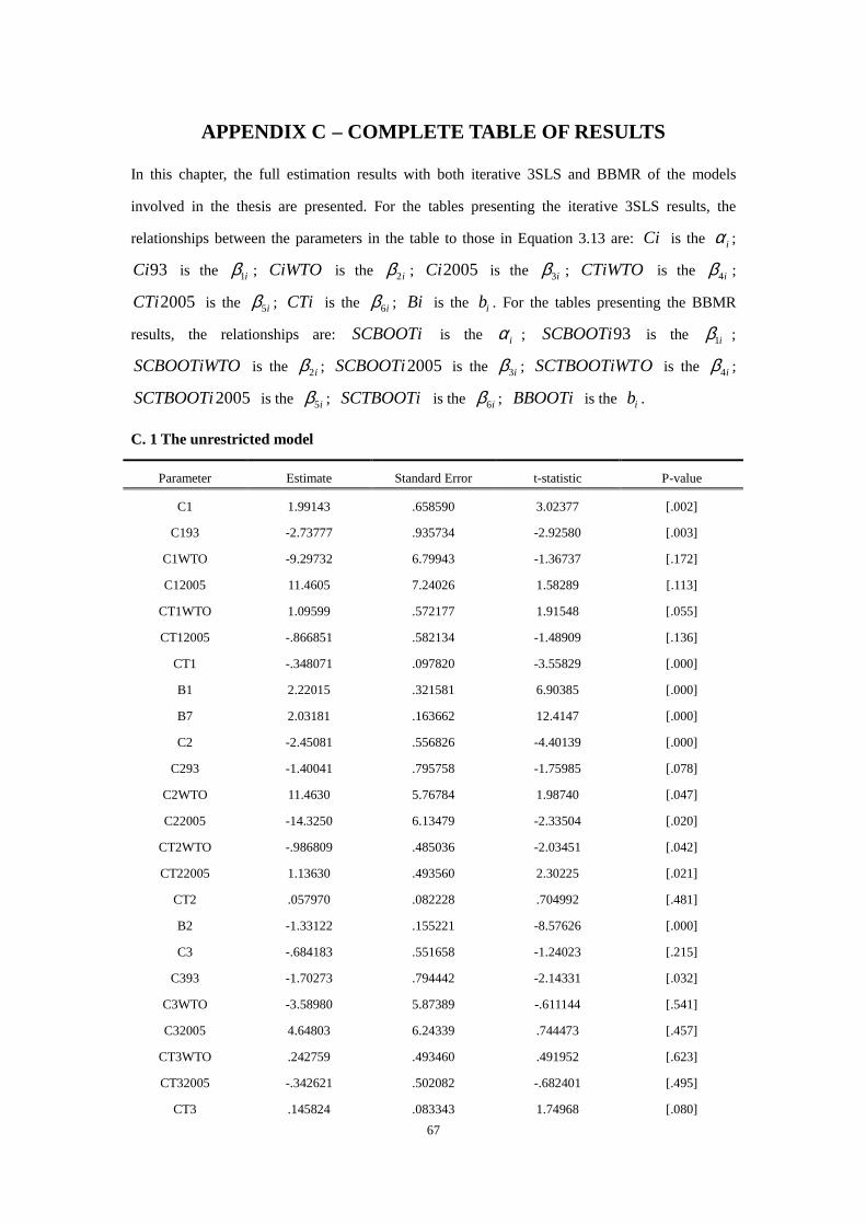
67

APPENDIX C – COMPLETE TABLE OF RESULTS

In this chapter, the full estimation results with both iterative 3SLS and BBMR of the models

involved in the thesis are presented. For the tables presenting the iterative 3SLS results, the

relationships between the parameters in the table to those in Equation 3.13 are: Ci is the iα ;

93Ci is the i1β ; CiWTO is the i2β ; 2005Ci is the i3β ; CTiWTO is the i4β ;

2005CTi is the i5β ; CTi is the i6β ; Bi is the ib . For the tables presenting the BBMR

results, the relationships are: SCBOOTi is the iα ; 93SCBOOTi is the i1β ;

SCBOOTiWTO is the i2β ; 2005SCBOOTi is the i3β ; OSCTBOOTiWT is the i4β ;

2005SCTBOOTi is the i5β ; SCTBOOTi is the i6β ; BBOOTi is the ib .

C. 1 The unrestricted model

Parameter Estimate Standard Error t-statistic P-value

C1 1.99143 .658590 3.02377 [.002]

C193 -2.73777 .935734 -2.92580 [.003]

C1WTO -9.29732 6.79943 -1.36737 [.172]

C12005 11.4605 7.24026 1.58289 [.113]

CT1WTO 1.09599 .572177 1.91548 [.055]

CT12005 -.866851 .582134 -1.48909 [.136]

CT1 -.348071 .097820 -3.55829 [.000]

B1 2.22015 .321581 6.90385 [.000]

B7 2.03181 .163662 12.4147 [.000]

C2 -2.45081 .556826 -4.40139 [.000]

C293 -1.40041 .795758 -1.75985 [.078]

C2WTO 11.4630 5.76784 1.98740 [.047]

C22005 -14.3250 6.13479 -2.33504 [.020]

CT2WTO -.986809 .485036 -2.03451 [.042]

CT22005 1.13630 .493560 2.30225 [.021]

CT2 .057970 .082228 .704992 [.481]

B2 -1.33122 .155221 -8.57626 [.000]

C3 -.684183 .551658 -1.24023 [.215]

C393 -1.70273 .794442 -2.14331 [.032]

C3WTO -3.58980 5.87389 -.611144 [.541]

C32005 4.64803 6.24339 .744473 [.457]

CT3WTO .242759 .493460 .491952 [.623]

CT32005 -.342621 .502082 -.682401 [.495]

CT3 .145824 .083343 1.74968 [.080]

68

B3 .054441 .150468 .361813 [.717]

C4 -3.15701 .476070 -6.63141 [.000]

C493 -.935867 .593972 -1.57561 [.115]

C4WTO -2.38915 4.75629 -.502313 [.615]

C42005 2.51739 4.87499 .516388 [.606]

CT4WTO -.013501 .401341 -.033640 [.973]

CT42005 -.131253 .389479 -.336996 [.736]

CT4 .293350 .067721 4.33177 [.000]

B4 3.98300 .342614 11.6253 [.000]

C5 -4.97076 .793891 -6.26127 [.000]

C593 1.61081 .822173 1.95921 [.050]

C5WTO 13.8005 5.71906 2.41306 [.016]

C52005 -17.6899 6.12866 -2.88642 [.004]

CT5WTO -1.48349 .491485 -3.01839 [.003]

CT52005 1.38120 .489332 2.82262 [.005]

CT5 .527411 .092014 5.73183 [.000]

B5 -4.99523 .743205 -6.72120 [.000]

C6 3.22522 .445803 7.23463 [.000]

C693 -2.50142 .662666 -3.77479 [.000]

C6WTO -10.7966 4.71899 -2.28791 [.022]

C62005 12.7225 5.02020 2.53426 [.011]

CT6WTO .979523 .396592 2.46985 [.014]

CT62005 -.954656 .403457 -2.36619 [.018]

CT6 -.167451 .067262 -2.48952 [.013]

B6 3.70171 .302450 12.2391 [.000]

Table C.1 Results of the unrestricted model with iterative 3SLS

C. 2 The 1st separable structure

C. 2. 1 Results with iterative 3SLS


C1 -.847760 .514582 -1.64747 [.099]

C193 -.207216 .705890 -.293553 [.769]

C1WTO -8.45848 5.91953 -1.42891 [.153]

C12005 11.2897 6.25841 1.80393 [.071]

CT1WTO .865470 .498145 1.73739 [.082]

CT12005 -.899779 .504362 -1.78400 [.074]

CT1 -.070430 .076005 -.926649 [.354]

69

B1 -.828551 .221555 -3.73971 [.000]

B7 1.34382 .237033 5.66932 [.000]

C2 -2.29763 .620814 -3.70099 [.000]

C293 -1.69596 .832140 -2.03807 [.042]

C2WTO 14.8927 6.74431 2.20819 [.027]

C22005 -16.8409 7.13093 -2.36168 [.018]

CT2WTO -1.26782 .568548 -2.22993 [.026]

CT22005 1.34274 .575215 2.33432 [.020]

CT2 .061095 .087138 .701125 [.483]

C3 -1.07122 .561680 -1.90717 [.056]

C393 -1.17128 .773105 -1.51504 [.130]

C3WTO 1.60467 6.55290 .244880 [.807]

C32005 -.696885 6.94662 -.100320 [.920]

CT3WTO -.159100 .551160 -.288664 [.773]

CT32005 .055957 .559857 .099950 [.920]

CT3 .194548 .083392 2.33295 [.020]

B3 -.636689 .219576 -2.89963 [.004]

C4 -1.02138 .598645 -1.70616 [.088]

C493 .411641 .778928 .528471 [.597]

C4WTO -24.0524 6.90577 -3.48295 [.000]

C42005 20.1734 7.18561 2.80747 [.005]

CT4WTO 1.85166 .581909 3.18205 [.001]

CT42005 -1.48164 .578180 -2.56260 [.010]

CT4 .031490 .087503 .359867 [.719]

C5 -.317491 .588468 -.539521 [.590]

C593 -1.30934 .695646 -1.88220 [.060]

C5WTO -3.72526 5.79219 -.643152 [.520]

C52005 3.66418 6.04728 .605921 [.545]

CT5WTO .212307 .491287 .432145 [.666]

CT52005 -.265500 .486582 -.545643 [.585]

CT5 .143748 .077845 1.84659 [.065]

C6 2.59652 .370996 6.99879 [.000]

C693 -3.30811 .443281 -7.46278 [.000]

C6WTO -7.87778 4.02311 -1.95813 [.050]

C62005 7.93384 4.21340 1.88300 [.060]

CT6WTO .730809 .339440 2.15299 [.031]

CT62005 -.622745 .338439 -1.84005 [.066]

CT6 -.129083 .051373 -2.51265 [.012]

70

Table C.2 Results of the 1st separable structure with iterative 3SLS

C. 2. 2 Results with BBMR

Parameter Mean Std. Dev. Minimum Maximum

SCBOOT1 -0.72478 0.15782 -0.99961 -0.17807

SCBOOT193 -0.42243 0.12843 -0.92071 -0.20586

SCBOOT1WTO 0.62760 0.86773 -2.53296 2.20852

SCBOOT12005 3.02219 0.62783 0.94971 5.51455

SCTBOOT1WTO 0.14432 0.074462 0.011654 0.40990

SCTBOOT12005 -0.22496 0.048815 -0.41828 -0.049343

SCTBOOT1 -0.076447 0.016581 -0.13792 -0.047847

SCBOOT2 -1.31126 0.19582 -1.65846 -0.55122

SCBOOT293 -2.81021 0.18959 -3.53748 -2.47338

SCBOOT2WTO 8.37600 0.90748 4.96493 10.63429

SCBOOT22005 -9.76219 0.78781 -12.39556 -6.60424

SCTBOOT2WTO -0.68560 0.080377 -0.87387 -0.39118

SCTBOOT22005 0.74574 0.063275 0.51034 0.96905

SCTBOOT2 -0.015084 0.018349 -0.082138 0.022928

SCBOOT3 -1.90331 0.20185 -2.30406 -1.40504

SCBOOT393 -0.91365 0.10852 -1.23816 -0.67152

SCBOOT3WTO 1.16774 0.71533 -1.55956 3.37439

SCBOOT32005 1.98065 0.60705 -0.56363 3.98026

SCTBOOT3WTO -0.20343 0.066543 -0.42589 0.030527

SCTBOOT32005 -0.13932 0.047448 -0.29949 0.070339

SCTBOOT3 0.26124 0.017007 0.20532 0.30237

SCBOOT4 -2.49578 0.31372 -3.12120 -1.76993

SCBOOT493 0.77865 0.11588 0.45810 1.03230

SCBOOT4WTO -12.79998 2.07278 -17.90339 -7.36050

SCBOOT42005 12.17527 1.59434 7.35001 17.08019

SCTBOOT4WTO 0.86983 0.17952 0.39438 1.29446

SCTBOOT42005 -0.84670 0.12025 -1.19551 -0.47123

SCTBOOT4 0.20297 0.034215 0.11009 0.27595

SCBOOT5 -1.70701 0.39340 -2.40651 -0.85173

SCBOOT593 -0.32944 0.27726 -0.93221 0.16355

SCBOOT5WTO 4.58212 1.62340 1.05274 7.46869

SCBOOT52005 -4.22624 1.40302 -6.72095 -1.17599

SCTBOOT5WTO -0.52861 0.14926 -0.79401 -0.20412

SCTBOOT52005 0.34836 0.10712 0.11548 0.53883

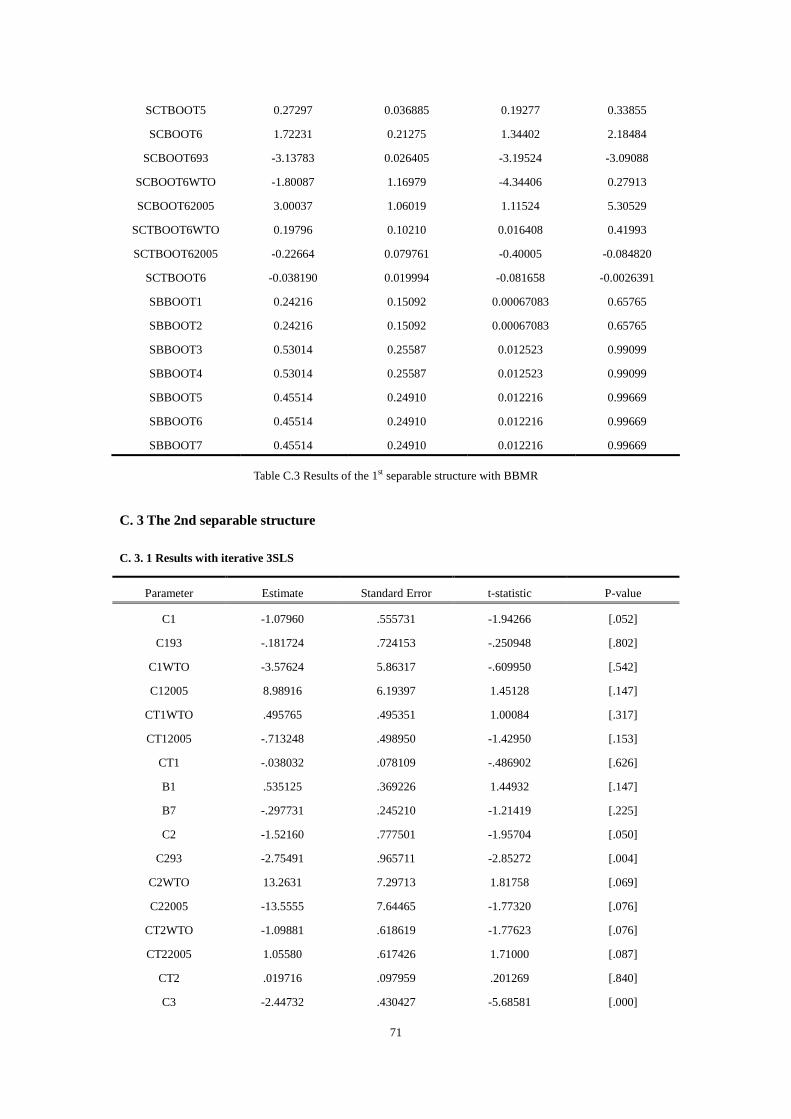
71

SCTBOOT5 0.27297 0.036885 0.19277 0.33855

SCBOOT6 1.72231 0.21275 1.34402 2.18484

SCBOOT693 -3.13783 0.026405 -3.19524 -3.09088

SCBOOT6WTO -1.80087 1.16979 -4.34406 0.27913

SCBOOT62005 3.00037 1.06019 1.11524 5.30529

SCTBOOT6WTO 0.19796 0.10210 0.016408 0.41993

SCTBOOT62005 -0.22664 0.079761 -0.40005 -0.084820

SCTBOOT6 -0.038190 0.019994 -0.081658 -0.0026391

SBBOOT1 0.24216 0.15092 0.00067083 0.65765

SBBOOT2 0.24216 0.15092 0.00067083 0.65765

SBBOOT3 0.53014 0.25587 0.012523 0.99099

SBBOOT4 0.53014 0.25587 0.012523 0.99099

SBBOOT5 0.45514 0.24910 0.012216 0.99669

SBBOOT6 0.45514 0.24910 0.012216 0.99669

SBBOOT7 0.45514 0.24910 0.012216 0.99669

Table C.3 Results of the 1st separable structure with BBMR

C. 3 The 2nd separable structure



C1 -1.07960 .555731 -1.94266 [.052]

C193 -.181724 .724153 -.250948 [.802]

C1WTO -3.57624 5.86317 -.609950 [.542]

C12005 8.98916 6.19397 1.45128 [.147]

CT1WTO .495765 .495351 1.00084 [.317]

CT12005 -.713248 .498950 -1.42950 [.153]

CT1 -.038032 .078109 -.486902 [.626]

B1 .535125 .369226 1.44932 [.147]

B7 -.297731 .245210 -1.21419 [.225]

C2 -1.52160 .777501 -1.95704 [.050]

C293 -2.75491 .965711 -2.85272 [.004]

C2WTO 13.2631 7.29713 1.81758 [.069]

C22005 -13.5555 7.64465 -1.77320 [.076]

CT2WTO -1.09881 .618619 -1.77623 [.076]

CT22005 1.05580 .617426 1.71000 [.087]

CT2 .019716 .097959 .201269 [.840]

C3 -2.44732 .430427 -5.68581 [.000]

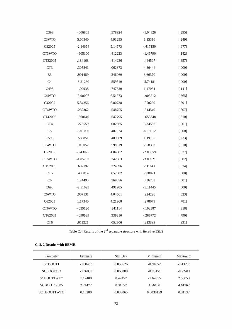
72

C393 -.606865 .578924 -1.04826 [.295]

C3WTO 5.66540 4.91295 1.15316 [.249]

C32005 -2.14654 5.14573 -.417150 [.677]

CT3WTO -.605100 .412223 -1.46790 [.142]

CT32005 .184168 .414236 .444597 [.657]

CT3 .305841 .062873 4.86444 [.000]

B3 .901489 .246060 3.66370 [.000]

C4 -3.21260 .559510 -5.74181 [.000]

C493 1.09938 .747620 1.47051 [.141]

C4WTO -5.90007 6.51573 -.905512 [.365]

C42005 5.84256 6.80738 .858269 [.391]

CT4WTO .282362 .548755 .514549 [.607]

CT42005 -.360640 .547795 -.658348 [.510]

CT4 .275559 .082365 3.34556 [.001]

C5 -3.01006 .487924 -6.16912 [.000]

C593 .583851 .489869 1.19185 [.233]

C5WTO 10.3052 3.98819 2.58393 [.010]

C52005 -8.43025 4.04602 -2.08359 [.037]

CT5WTO -1.05763 .342363 -3.08921 [.002]

CT52005 .687192 .324696 2.11641 [.034]

CT5 .403814 .057682 7.00071 [.000]

C6 1.24493 .369676 3.36763 [.001]

C693 -2.51623 .491985 -5.11445 [.000]

C6WTO .907131 4.04561 .224226 [.823]

C62005 1.17340 4.21968 .278079 [.781]

CT6WTO -.035130 .341114 -.102987 [.918]

CT62005 -.090599 .339610 -.266772 [.790]

CT6 .011225 .052606 .213383 [.831]

Table C.4 Results of the 2nd separable structure with iterative 3SLS


Parameter Estimate Std. Dev Minimum Maximum

SCBOOT1 -0.80463 0.059626 -0.94052 -0.43288

SCBOOT193 -0.36859 0.065800 -0.75151 -0.22411

SCBOOT1WTO 1.12400 0.42452 -1.62815 2.50053

SCBOOT12005 2.74472 0.31052 1.56100 4.61362

SCTBOOT1WTO 0.10280 0.033065 0.0030159 0.31137

73

SCTBOOT12005 -0.20348 0.024968 -0.34861 -0.11219

SCTBOOT1 -0.068044 0.0066222 -0.11729 -0.050866

SCBOOT2 -1.35325 0.15400 -1.65365 -0.62328

SCBOOT293 -2.79753 0.18326 -3.56987 -2.43122

SCBOOT2WTO 8.67905 0.57043 6.17294 10.13795

SCBOOT22005 -9.87955 0.65020 -11.82465 -7.68297

SCTBOOT2WTO -0.71125 0.052070 -0.83704 -0.47714

SCTBOOT22005 0.75361 0.054641 0.56897 0.90964

SCTBOOT2 -0.0093550 0.011749 -0.083897 0.018227

SCBOOT3 -2.03641 0.13705 -2.35951 -1.60609

SCBOOT393 -0.88346 0.10125 -1.16255 -0.64267

SCBOOT3WTO 1.23506 0.72036 -1.07944 3.61305

SCBOOT32005 2.13748 0.59393 0.057397 3.95937

SCTBOOT3WTO -0.22238 0.062241 -0.43404 -0.024465

SCTBOOT32005 -0.15079 0.046621 -0.28950 0.031564

SCTBOOT3 0.27013 0.013883 0.23364 0.30975

SCBOOT4 -2.73451 0.17363 -3.07703 -2.03865

SCBOOT493 0.82105 0.10146 0.55253 1.06050

SCBOOT4WTO -11.21270 1.13923 -16.00641 -7.81802

SCBOOT42005 10.96311 0.88554 7.98742 14.19405

SCTBOOT4WTO 0.73194 0.098426 0.44246 1.13636

SCTBOOT42005 -0.75550 0.068140 -0.99683 -0.50599

SCTBOOT4 0.22902 0.018980 0.15864 0.27289

SCBOOT5 -1.95548 0.26643 -2.41878 -0.94233

SCBOOT593 -0.15432 0.18777 -0.86836 0.17220

SCBOOT5WTO 5.60745 1.09945 1.42660 7.51932

SCBOOT52005 -5.11238 0.95019 -6.76471 -1.49910

SCTBOOT5WTO -0.62288 0.10108 -0.79866 -0.23849

SCTBOOT52005 0.41602 0.072546 0.14015 0.54217

SCTBOOT5 0.29626 0.024981 0.20127 0.33970

SCBOOT6 1.62608 0.13097 1.30806 2.01845

SCBOOT693 -2.90867 0.14266 -3.48919 -2.57363

SCBOOT6WTO -1.49822 0.73039 -4.08878 1.08181

SCBOOT62005 3.15267 0.57433 0.97503 4.83535

SCTBOOT6WTO 0.17023 0.063315 -0.051281 0.38768

SCTBOOT62005 -0.23721 0.045224 -0.36488 -0.047115

SCTBOOT6 -0.025738 0.014453 -0.065495 0.013713

SBBOOT1 0.29476 0.17688 0.00016773 0.85024

74

SBBOOT2 0.29476 0.17688 0.00016773 0.85024

SBBOOT3 0.74349 0.13224 0.16912 0.99614

SBBOOT4 0.74349 0.13224 0.16912 0.99614

SBBOOT5 0.29781 0.16870 0.0044466 0.93932

SBBOOT6 0.74349 0.13224 0.16912 0.99614

Table C.5 Results of the 2nd separable structure with BBMR

C. 4 The 3rd separable structure



C1 -.865502 .606609 -1.42679 [.154]

C193 -.393425 .767351 -.512706 [.608]

C1WTO -3.86654 6.12595 -.631175 [.528]

C12005 9.55720 6.45363 1.48090 [.139]

CT1WTO .538832 .518900 1.03841 [.299]

CT12005 -.757090 .519721 -1.45672 [.145]

CT1 -.058462 .083226 -.702455 [.482]

B1 .961036 .400071 2.40216 [.016]

B7 -.451963 .257141 -1.75765 [.079]

C2 -.992723 .840204 -1.18153 [.237]

C293 -3.30531 1.00643 -3.28418 [.001]

C2WTO 10.9390 7.42914 1.47245 [.141]

C22005 -11.2428 7.71316 -1.45761 [.145]

CT2WTO -.887492 .631655 -1.40502 [.160]

CT22005 .864085 .623171 1.38659 [.166]

CT2 -.023757 .101776 -.233425 [.815]

C3 -2.56202 .433456 -5.91068 [.000]

C393 -.453318 .578126 -.784116 [.433]

C3WTO 7.01488 4.90625 1.42978 [.153]

C32005 -3.29405 5.13167 -.641907 [.521]

CT3WTO -.710751 .411649 -1.72660 [.084]

CT32005 .273473 .413048 .662086 [.508]

CT3 .322810 .062906 5.13165 [.000]

B3 .695808 .264895 2.62673 [.009]

C4 -3.21830 .592610 -5.43072 [.000]

C493 1.23644 .787911 1.56926 [.117]

C4WTO -6.43489 6.89186 -.933694 [.350]

75

C42005 6.41748 7.19219 .892285 [.372]

CT4WTO .326915 .580510 .563152 [.573]

CT42005 -.404088 .578695 -.698275 [.485]

CT4 .274773 .087094 3.15491 [.002]

C5 -3.26304 .503778 -6.47714 [.000]

C593 .761726 .497092 1.53237 [.125]

C5WTO 11.6234 4.03519 2.88051 [.004]

C52005 -9.56659 4.07756 -2.34615 [.019]

CT5WTO -1.17695 .346945 -3.39231 [.001]

CT52005 .776702 .327105 2.37448 [.018]

CT5 .428249 .058890 7.27200 [.000]

C6 1.12699 .384624 2.93012 [.003]

C693 -2.39291 .534497 -4.47694 [.000]

C6WTO 1.62448 4.20566 .386260 [.699]

C62005 .736821 4.41108 .167039 [.867]

CT6WTO -.097964 .354623 -.276249 [.782]

CT62005 -.055365 .354572 -.156146 [.876]

CT6 .024314 .054630 .445062 [.656]

Table C.6 Results of the 3rd separable structure with iterative 3SLS


Parameter Estimate Std. Dev Minimum Maximum

SCBOOT1 -0.67324 0.13498 -1.13042 -0.24571

SCBOOT193 -0.49251 0.12582 -0.89692 -0.097373

SCBOOT1WTO 0.86322 0.62198 -1.57167 2.38915

SCBOOT12005 3.14046 0.55463 1.59768 4.83522

SCTBOOT1WTO 0.13501 0.054405 -0.016802 0.33205

SCTBOOT12005 -0.23407 0.043044 -0.36309 -0.11124

SCTBOOT1 -0.080452 0.013861 -0.13540 -0.036864

SCBOOT2 -1.05358 0.27469 -1.86205 -0.29636

SCBOOT293 -3.10440 0.28902 -3.87682 -2.32737

SCBOOT2WTO 7.55891 1.05365 4.55386 10.87877

SCBOOT22005 -8.77223 1.06717 -11.80045 -5.85908

SCTBOOT2WTO -0.60849 0.095851 -0.90757 -0.33793

SCTBOOT22005 0.66251 0.087429 0.42743 0.90663

SCTBOOT2 -0.033646 0.022588 -0.11188 0.034748

SCBOOT3 -2.06980 0.15450 -2.34715 -1.52421

SCBOOT393 -0.77109 0.11720 -1.17898 -0.56915

76

SCBOOT3WTO 2.07373 0.83498 -0.33842 3.65881

SCBOOT32005 1.34059 0.74286 -0.15794 3.92403

SCTBOOT3WTO -0.28077 0.068228 -0.39923 -0.056418

SCTBOOT32005 -0.090715 0.056952 -0.27944 0.023682

SCTBOOT3 0.27906 0.015388 0.22321 0.30972

SCBOOT4 -2.64288 0.23323 -3.15854 -1.91929

SCBOOT493 0.91898 0.11426 0.49939 1.11716

SCBOOT4WTO -12.17296 1.61534 -17.41137 -8.34684

SCBOOT42005 11.78646 1.27209 8.79576 15.99187

SCTBOOT4WTO 0.81432 0.13970 0.48284 1.26902

SCTBOOT42005 -0.81694 0.095815 -1.13820 -0.58058

SCTBOOT4 0.21764 0.025821 0.13494 0.27646

SCBOOT5 -2.05719 0.30216 -2.42481 -0.91883

SCBOOT593 -0.082638 0.21296 -0.88492 0.17645

SCBOOT5WTO 6.02719 1.24690 1.32964 7.54421

SCBOOT52005 -5.47514 1.07763 -6.78622 -1.41530

SCTBOOT5WTO -0.66147 0.11464 -0.80095 -0.22958

SCTBOOT52005 0.44372 0.082276 0.13375 0.54382

SCTBOOT5 0.30580 0.028331 0.19907 0.34027

SCBOOT6 1.56070 0.13550 1.30126 2.04973

SCBOOT693 -2.97100 0.21583 -3.71737 -2.50545

SCBOOT6WTO -1.05499 0.68454 -3.90351 0.56583

SCBOOT62005 2.59145 0.52163 1.04646 4.40921

SCTBOOT6WTO 0.13206 0.059882 -0.0052918 0.38186

SCTBOOT62005 -0.19564 0.040434 -0.33848 -0.066747

SCTBOOT6 -0.020770 0.015879 -0.080449 0.022186

SBBOOT1 0.52855 0.23922 0.0068842 0.99885

SBBOOT2 0.52855 0.23922 0.0068842 0.99885

SBBOOT3 0.49099 0.24856 0.0047872 0.99441

SBBOOT4 0.49099 0.24856 0.0047872 0.99441

SBBOOT5 0.23340 0.19133 0.00062770 0.95420

SBBOOT6 0.52855 0.23922 0.0068842 0.99885

SBBOOT7 0.23340 0.19133 0.00062770 0.95420

Table C.7 Results of the 3rd separable structure with BBMR

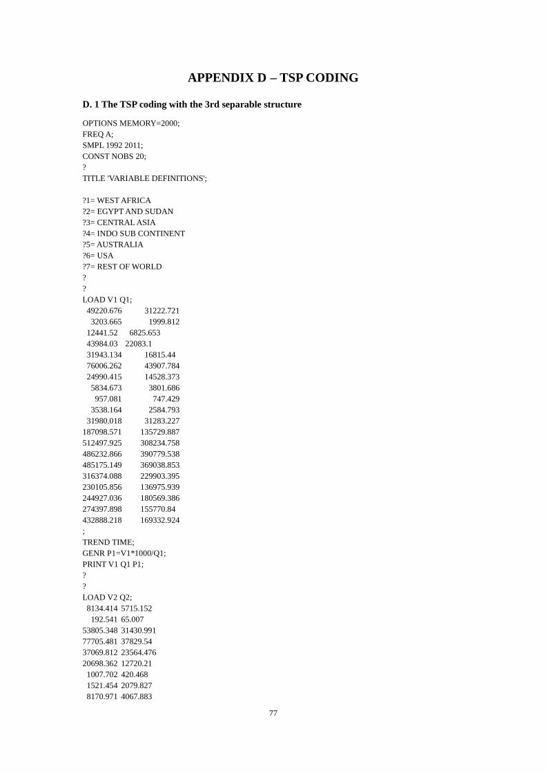
77

APPENDIX D – TSP CODING

D. 1 The TSP coding with the 3rd separable structure

OPTIONS MEMORY=2000; FREQ A; SMPL 1992 2011; CONST NOBS 20; ? TITLE 'VARIABLE DEFINITIONS'; ?1= WEST AFRICA ?2= EGYPT AND SUDAN ?3= CENTRAL ASIA ?4= INDO SUB CONTINENT ?5= AUSTRALIA ?6= USA ?7= REST OF WORLD ? ? LOAD V1 Q1; 49220.676 31222.721 3203.665 1999.812 12441.52 6825.653 43984.03 22083.1 31943.134 16815.44 76006.262 43907.784 24990.415 14528.373 5834.673 3801.686 957.081 747.429 3538.164 2584.793 31980.018 31283.227 187098.571 135729.887 512497.925 308234.758 486232.866 390779.538 485175.149 369038.853 316374.088 229903.395 230105.856 136975.939 244927.036 180569.386 274397.898 155770.84 432888.218 169332.924 ; TREND TIME; GENR P1=V1*1000/Q1; PRINT V1 Q1 P1; ? ? LOAD V2 Q2; 8134.414 5715.152 192.541 65.007 53805.348 31430.991 77705.481 37829.54 37069.812 23564.476 20698.362 12720.21 1007.702 420.468 1521.454 2079.827 8170.971 4067.883

78

5208.626 2064.818 10536.189 5075.735 17966.101 9946.279 32148.306 15728.383 38931.879 21138.3 35574.274 14796.958 24329.122 10248.425 21509.433 8921.349 27260.42 11694.539 67051.801 23435.872 92233.659 20898.123 ; GENR P2=V2*1000/Q2; PRINT V2 Q2 P2; ? LOAD V3 Q3; 3268.297 7115.957 1410.287 3014.025 92551.97 91064.938 128624.626 248387.476 92050.176 91746.716 198616.431 128578.079 54477.466 79122.662 18991.074 60397.398 24749.272 87675.716 10872.437 31181.393 24532.992 29111.368 191569.283 176805.807 358854.985 255980.876 417297.918 375245.709 556985.604 475324.941 332242.865 288243.834 305289.57 217317.578 202324.872 200611.577 757460.69 422422.593 559711.239 205069.017 ; GENR P3=V3*1000/Q3; PRINT V3 Q3 P3; ? ? LOAD V4 Q4; 27542.032 18979.892 4366.697 4961.42 9500.356 10069.236 11164.696 7827.255 77929.04 46801.642 43866.273 30371.373 13820.935 14733.498 2467.94 7837.772 11619.379 28870.74 12221.04 28911.601 444.914 1408.481 8680.425 15178.48 82179.08 60227.151 169950.406 150651.244 784144.229 637658.544 888925.674 680155.12

79

983404.277 643818.166 493507.073 383274.98 1861357.617 968442.931 2805763.442 1110873.788 ; GENR P4=V4*1000/Q4; PRINT V4 Q4 P4; ? LOAD V5 Q5; 6450.296 4289.597 2419.948 1777.187 73786.576 40050.016 50570.192 23782.936 73611.056 39434.064 187835.648 101203.232 50900.728 30459.252 25688.45 17524.581 18021.072 13042.439 25245.626 21129.198 23575.571 19949.644 36335.257 24257.634 176852.555 102983.74 274992.503 202638.804 318402.552 227948.617 171702.084 117199.88 133691.173 77037.218 148794.408 102491.544 415792.229 204918.1 1549105.63 529687.275 ; GENR P5=V5*1000/Q5; PRINT V5 Q5 P5; ? LOAD V6 Q6; 273468.736 170574.464 1998.436 3803.288 551302.912 317836.896 964342.144 521284.768 803832.128 423381.504 725273.152 420764.544 195003.6 134663.088 26733.786 33246.815 58683.336 72500.555 50636.182 63796.205 92672.655 105175.531 666387.525 529455.53 1782180.804 1091630.801 1471545.67 1213250.332 2302777.003 1747803.744 1615187.655 1154368.382 1666913.921 994313.98 891642.286 681812.344 2016425.988 1035592.043 2979460.099 1014148.542 ; GENR P6=V6*1000/Q6; PRINT V6 Q6 P6;

80

? LOAD VWORLD QWORLD; 457584.96 326955.296 25199.434 44775.296 936139.776 615757.056 1486725.76 1003366.592 1276438.016 751459.648 1410343.168 848835.264 381343.84 310285.728 104825.974 163871.814 137197.321 250906.032 116608.617 197097.699 199511.78 245061.35 1218245.977 1074961.058 3242122.824 2114129.012 3246197.095 2745287.768 4974642.693 3980021.554 3579753.596 2740434.396 3564706.744 2263696.391 2211367.939 1758926.167 5846449.51 3127633.895 9678595.164 3566339.643 ; GENR PWORLD=VWORLD*1000/QWORLD; PRINT VWORLD QWORLD PWORLD; ? GENR V7=VWORLD-V1-V2-V3-V4-V5-V6; GENR Q7=QWORLD-Q1-Q2-Q3-Q4-Q5-Q6; GENR P7=V7*1000/Q7; PRINT V7 Q7 P7; ? GENR VTOT=V1+V2+V3+V4+V5+V6+V7; DOT 1-7; NORMAL P.,2000,1; ENDDOT; PRINT P1-P7; DOT 1-7; GENR S.=V./VTOT; MSD S.; SET SM.=@MEAN(1); ENDDOT; PRINT P1-P7; GENR TOTALS=S1+S2+S3+S4+S5+S6+S7; PRINT S1-S7 TOTALS; ? LOAD DUM1993; 0 1 0 0 0 0 0 0 0 0 0 0 0 0 0 0 0 0 0 0; LOAD DUMWTO; 0 0 0 0 0 0 0 0 0 1 1 1 1 1 1 1 1 1 1 1; LOAD DUMWTO1; 0 0 0 0 0 0 0 0 0 0 1 1 1 1 1 1 1 1

81

1 1; LOAD DUM2005; 0 0 0 0 0 0 0 0 0 0 0 0 0 1 1 1 1 1 1 1; PRINT DUM1993 DUMWTO DUMWTO1 DUM2005; ? SMPL 1992 2011; DOT 1-6; Y.=LOG(S.)-LOG(S7); ENDDOT; PRINT Y1-Y6; ? TITLE 'STONE PRICE INDEX WITH CURRENT "BUDGET SHARES'; GENR PSTONE_CUR=EXP(S1*LOG(P1)+S2*LOG(P2)+S3*LOG(P3)+S3*LOG(P4)+S5*LOG(P5)+S6*LOG(P6)+S7*LOG(P7)); PRINT PSTONE_CUR; DOT 1-7; GENR LP.=LOG(P.); ENDDOT; PRINT LP1-LP7; GENR LP=LOG(PSTONE_CUR); PRINT LP; GENR DUMWTO_TIME=DUMWTO1*TIME; GENR DUM2005_TIME=DUM2005*TIME; ? TITLE 'CDEH MODEL FOR CHINESE IMPORTS'; ? DOT 1-6; FRML EQ. Y.=C.+C.93*DUM1993+(C.WTO*DUMWTO1+C.2005*DUM2005)+ +(CT.WTO*DUMWTO1+CT.2005*DUM2005)*TIME+CT.*TIME +B.*(LP.-LP)-B7*(LP7-LP); GENR DUMWTO_TIME=DUMWTO1*TIME; GENR DUM2005_TIME=DUM2005*TIME; PRINT EQ.; ENDDOT; PARAM C193-C693; PARAM CT1-CT6; PARAM CT1WTO-CT6WTO; PARAM CT12005 CT22005 CT32005 CT42005 CT52005 CT62005; PARAM B1-B7; PARAM C1-C6; PARAM C1WTO-C6WTO; PARAM C12005 C22005 C32005 C42005 C52005 C62005; ? SMPL 1992 2011; PRINT Y1-Y6; DOT 1-6; LSQ EQ.;

82

ENDDOT; ? LSQ(MAXIT=1000,MAXITW=200)EQ1-EQ6; LSQ(MAXIT=1000,MAXITW=200,INST=(C,LP1-LP7,DUM1993,DUMWTO1,DUM2005,TIME,DUMWTO_TIME,DUM2005_TIME))EQ1-EQ6; ?CONST C12005 0 C22005 0 C32005 0 C42005 0 C52005 0 C62005 0; ?LSQ(MAXIT=200)EQ1-EQ6; ? ? TITLE 'SEPARABILITY BETWEEN "AFRICA, US", "ASIA" AND "AUSTRAILA, RESTOF"'; FRML EQSEP2 B2=B1; FRML EQSEP4 B4=B3; FRML EQSEP5 B5=B7; FRML EQSEP6 B6=B1; EQSUB(PRINT)EQ2 EQSEP2; EQSUB(PRINT)EQ4 EQSEP4; EQSUB(PRINT)EQ5 EQSEP5; EQSUB(PRINT)EQ6 EQSEP6; PRINT EQ1-EQ6; LSQ(MAXIT=1000,MAXITW=200,INST=(C,LP1-LP7,DUM1993,DUMWTO1,DUM2005,TIME))EQ1-EQ6; ? LOAD CONST; 1 1 1 1 1 1 1 1 1 1 1 1 1 1 1 1 1 1 1 1; ?All EXOGENOUS VARIABLES MMAKE X CONST DUM1993 DUMWTO1 DUM2005 DUMWTO_TIME DUM2005_TIME TIME LP1 LP2 LP3 LP4 LP5 LP6 LP7; MAT INVX=(X'X)"X'; MAT XINVX=X*INVX; ?ENDOGENOUS VARIABLES MMAKE Z LP; MAT MEANPI=INVX*Z; MAT EHAT=Z-X*MEANPI; PRINT EHAT; MAT S=EHAT'EHAT; PRINT S; ?SQUARE ROOT OF S MAT EIGVAS=EIGVAL(S); PRINT EIGVAS; MAT EIGVES=EIGVEC(S); PRINT EIGVES; MAT SQS=EIGVES*SQRT(DIAG(EIGVAS))*EIGVES'; PRINT SQS; ? MAT M=IDENT(NOBS)-XINVX; PRINT M; ?BOOTSTRAP AND 3SLS MAPPING ? SET FLAG=0;

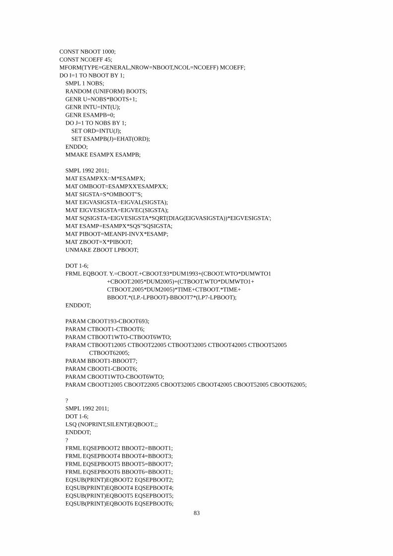
83

CONST NBOOT 1000; CONST NCOEFF 45; MFORM(TYPE=GENERAL,NROW=NBOOT,NCOL=NCOEFF) MCOEFF; DO I=1 TO NBOOT BY 1; SMPL 1 NOBS; RANDOM (UNIFORM) BOOTS; GENR U=NOBS*BOOTS+1; GENR INTU=INT(U); GENR ESAMPB=0; DO J=1 TO NOBS BY 1; SET ORD=INTU(J); SET ESAMPB(J)=EHAT(ORD); ENDDO; MMAKE ESAMPX ESAMPB; SMPL 1992 2011; MAT ESAMPXX=M*ESAMPX; MAT OMBOOT=ESAMPXX'ESAMPXX; MAT SIGSTA=S*OMBOOT"S; MAT EIGVASIGSTA=EIGVAL(SIGSTA); MAT EIGVESIGSTA=EIGVEC(SIGSTA); MAT SQSIGSTA=EIGVESIGSTA*SQRT(DIAG(EIGVASIGSTA))*EIGVESIGSTA'; MAT ESAMP=ESAMPX*SQS"SQSIGSTA; MAT PIBOOT=MEANPI-INVX*ESAMP; MAT ZBOOT=X*PIBOOT; UNMAKE ZBOOT LPBOOT; DOT 1-6; FRML EQBOOT. Y.=CBOOT.+CBOOT.93*DUM1993+(CBOOT.WTO*DUMWTO1 +CBOOT.2005*DUM2005)+(CTBOOT.WTO*DUMWTO1+ CTBOOT.2005*DUM2005)*TIME+CTBOOT.*TIME+ BBOOT.*(LP.-LPBOOT)-BBOOT7*(LP7-LPBOOT); ENDDOT; PARAM CBOOT193-CBOOT693; PARAM CTBOOT1-CTBOOT6; PARAM CTBOOT1WTO-CTBOOT6WTO; PARAM CTBOOT12005 CTBOOT22005 CTBOOT32005 CTBOOT42005 CTBOOT52005 CTBOOT62005; PARAM BBOOT1-BBOOT7; PARAM CBOOT1-CBOOT6; PARAM CBOOT1WTO-CBOOT6WTO; PARAM CBOOT12005 CBOOT22005 CBOOT32005 CBOOT42005 CBOOT52005 CBOOT62005; ? SMPL 1992 2011; DOT 1-6; LSQ (NOPRINT,SILENT)EQBOOT.;; ENDDOT; ? FRML EQSEPBOOT2 BBOOT2=BBOOT1; FRML EQSEPBOOT4 BBOOT4=BBOOT3; FRML EQSEPBOOT5 BBOOT5=BBOOT7; FRML EQSEPBOOT6 BBOOT6=BBOOT1; EQSUB(PRINT)EQBOOT2 EQSEPBOOT2; EQSUB(PRINT)EQBOOT4 EQSEPBOOT4; EQSUB(PRINT)EQBOOT5 EQSEPBOOT5; EQSUB(PRINT)EQBOOT6 EQSEPBOOT6;

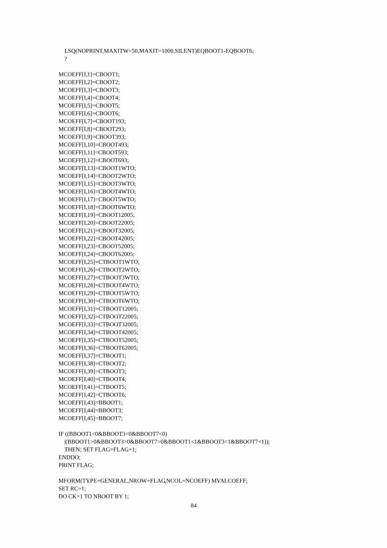
84

LSQ(NOPRINT,MAXITW=50,MAXIT=1000,SILENT)EQBOOT1-EQBOOT6; ? MCOEFF[I,1]=CBOOT1; MCOEFF[I,2]=CBOOT2; MCOEFF[I,3]=CBOOT3; MCOEFF[I,4]=CBOOT4; MCOEFF[I,5]=CBOOT5; MCOEFF[I,6]=CBOOT6; MCOEFF[I,7]=CBOOT193; MCOEFF[I,8]=CBOOT293; MCOEFF[I,9]=CBOOT393; MCOEFF[I,10]=CBOOT493; MCOEFF[I,11]=CBOOT593; MCOEFF[I,12]=CBOOT693; MCOEFF[I,13]=CBOOT1WTO; MCOEFF[I,14]=CBOOT2WTO; MCOEFF[I,15]=CBOOT3WTO; MCOEFF[I,16]=CBOOT4WTO; MCOEFF[I,17]=CBOOT5WTO; MCOEFF[I,18]=CBOOT6WTO; MCOEFF[I,19]=CBOOT12005; MCOEFF[I,20]=CBOOT22005; MCOEFF[I,21]=CBOOT32005; MCOEFF[I,22]=CBOOT42005; MCOEFF[I,23]=CBOOT52005; MCOEFF[I,24]=CBOOT62005; MCOEFF[I,25]=CTBOOT1WTO; MCOEFF[I,26]=CTBOOT2WTO; MCOEFF[I,27]=CTBOOT3WTO; MCOEFF[I,28]=CTBOOT4WTO; MCOEFF[I,29]=CTBOOT5WTO; MCOEFF[I,30]=CTBOOT6WTO; MCOEFF[I,31]=CTBOOT12005; MCOEFF[I,32]=CTBOOT22005; MCOEFF[I,33]=CTBOOT32005; MCOEFF[I,34]=CTBOOT42005; MCOEFF[I,35]=CTBOOT52005; MCOEFF[I,36]=CTBOOT62005; MCOEFF[I,37]=CTBOOT1; MCOEFF[I,38]=CTBOOT2; MCOEFF[I,39]=CTBOOT3; MCOEFF[I,40]=CTBOOT4; MCOEFF[I,41]=CTBOOT5; MCOEFF[I,42]=CTBOOT6; MCOEFF[I,43]=BBOOT1; MCOEFF[I,44]=BBOOT3; MCOEFF[I,45]=BBOOT7; IF ((BBOOT1<0&BBOOT3<0&BBOOT7<0) |(BBOOT1>0&BBOOT3>0&BBOOT7>0&BBOOT1<1&BBOOT3<1&BBOOT7<1)); THEN; SET FLAG=FLAG+1; ENDDO; PRINT FLAG; MFORM(TYPE=GENERAL,NROW=FLAG,NCOL=NCOEFF) MVALCOEFF; SET RC=1; DO CK=1 TO NBOOT BY 1;

85

IF ((MCOEFF[CK,43]<0&MCOEFF[CK,44]<0&MCOEFF[CK,45]<0)| (MCOEFF[CK,43]>0&MCOEFF[CK,44]>0&MCOEFF[CK,45]>0 &MCOEFF[CK,43]<1&MCOEFF[CK,44]<1&MCOEFF[CK,45]<1)); THEN; DO; DO CC=1 TO NCOEFF BY 1; MVALCOEFF[RC,CC]=MCOEFF[CK,CC]; ENDDO; SET RC=RC+1; ENDDO; ENDDO; FREQ NONE; SMPL 1 FLAG; UNMAKE MVALCOEFF SCBOOT1-SCBOOT6 SCBOOT193 SCBOOT293 SCBOOT393 SCBOOT493 SCBOOT593 SCBOOT693 SCBOOT1WTO-SCBOOT6WTO SCBOOT12005 SCBOOT22005 SCBOOT32005 SCBOOT42005 SCBOOT52005 SCBOOT62005 SCTBOOT1WTO-SCTBOOT6WTO SCTBOOT12005 SCTBOOT22005 SCTBOOT32005 SCTBOOT42005 SCTBOOT52005 SCTBOOT62005 SCTBOOT1-SCTBOOT6 SBBOOT1 SBBOOT3 SBBOOT7; GENR SBBOOT2=SBBOOT1; GENR SBBOOT4=SBBOOT3; GENR SBBOOT5=SBBOOT7; GENR SBBOOT6=SBBOOT1; ? POSTERIOR MEAN AND VARIANCE FOR ALL COEFFICIENTS DOT 1-6; MSD SCBOOT.; MSD SCBOOT.93; MSD SCBOOT.WTO; MSD SCBOOT.2005; MSD SCTBOOT.WTO; MSD SCTBOOT.2005; MSD SCTBOOT.; ENDDOT; ? DOT 1-7; MSD SBBOOT.; ENDDOT; DOT 1-7; GENR ALPHABOOT.=1-SBBOOT.; MSD ALPHABOOT.; ENDDOT; ? GENR ROTBOOT=ALPHABOOT1*SM1+ALPHABOOT2*SM2+ALPHABOOT3*SM3+ALPHABOOT4*SM4 +ALPHABOOT5*SM5+ALPHABOOT6*SM6+ALPHABOOT7*SM7; MSD ROTBOOT; ? TITLE 'ALLEN ELASTICITIES OF SUBSTITUTION'; TITLE 'SHORT RUN'; ? TITLE 'OWN PRICE ELASTICITIES OF SUBSTITUTION'; TITLE 'SHORT RUN'; ? GENR ALLENBOOT11=ALPHABOOT1+ALPHABOOT1-ROTBOOT-ALPHABOOT1/SM1; MSD ALLENBOOT11;

86

? GENR ALLENBOOT22=ALPHABOOT2+ALPHABOOT2-ROTBOOT-ALPHABOOT2/SM2; MSD ALLENBOOT22; ? GENR ALLENBOOT33=ALPHABOOT3+ALPHABOOT3-ROTBOOT-ALPHABOOT3/SM3; MSD ALLENBOOT33; ? GENR ALLENBOOT44=ALPHABOOT4+ALPHABOOT4-ROTBOOT-ALPHABOOT4/SM4; MSD ALLENBOOT44; ? GENR ALLENBOOT55=ALPHABOOT5+ALPHABOOT5-ROTBOOT-ALPHABOOT5/SM5; MSD ALLENBOOT55; ? GENR ALLENBOOT66=ALPHABOOT6+ALPHABOOT6-ROTBOOT-ALPHABOOT6/SM6; MSD ALLENBOOT66; ? GENR ALLENBOOT77=ALPHABOOT7+ALPHABOOT7-ROTBOOT-ALPHABOOT7/SM7; MSD ALLENBOOT77; ? DOT 2-7; GENR ALLENBOOT1.=ALPHABOOT1+ALPHABOOT.-ROTBOOT; MSD ALLENBOOT1.; ENDDOT; ? DOT 3-7; GENR ALLENBOOT2.=ALPHABOOT2+ALPHABOOT.-ROTBOOT; MSD ALLENBOOT2.; ENDDOT; ? DOT 4-7; GENR ALLENBOOT3.=ALPHABOOT3+ALPHABOOT.-ROTBOOT; MSD ALLENBOOT3.; ENDDOT; ? DOT 5-7; GENR ALLENBOOT4.=ALPHABOOT4+ALPHABOOT.-ROTBOOT; MSD ALLENBOOT4.; ENDDOT; ? DOT 6-7; GENR ALLENBOOT5.=ALPHABOOT5+ALPHABOOT.-ROTBOOT; MSD ALLENBOOT5.; ENDDOT; ? DOT 7; GENR ALLENBOOT6.=ALPHABOOT6+ALPHABOOT.-ROTBOOT; MSD ALLENBOOT6.; ENDDOT;

D. 2 The TSP coding for the HPD

OPTIONS MEMORY=2000; FREQ A; SMPL 1992 2011; CONST NOBS 20; ? TITLE 'VARIABLE DEFINITIONS';

87

?1= WEST AFRICA ?2= EGYPT AND SUDAN ?3= CENTRAL ASIA ?4= INDO SUB CONTINENT ?5= AUSTRALIA ?6= USA ?7= REST OF WORLD ? ? LOAD V1 Q1; 49220.676 31222.721 3203.665 1999.812 12441.52 6825.653 43984.03 22083.1 31943.134 16815.44 76006.262 43907.784 24990.415 14528.373 5834.673 3801.686 957.081 747.429 3538.164 2584.793 31980.018 31283.227 187098.571 135729.887 512497.925 308234.758 486232.866 390779.538 485175.149 369038.853 316374.088 229903.395 230105.856 136975.939 244927.036 180569.386 274397.898 155770.84 432888.218 169332.924 ; TREND TIME; GENR P1=V1*1000/Q1; PRINT V1 Q1 P1; ? ? LOAD V2 Q2; 8134.414 5715.152 192.541 65.007 53805.348 31430.991 77705.481 37829.54 37069.812 23564.476 20698.362 12720.21 1007.702 420.468 1521.454 2079.827 8170.971 4067.883 5208.626 2064.818 10536.189 5075.735 17966.101 9946.279 32148.306 15728.383 38931.879 21138.3 35574.274 14796.958 24329.122 10248.425 21509.433 8921.349 27260.42 11694.539 67051.801 23435.872 92233.659 20898.123 ;

88

GENR P2=V2*1000/Q2; PRINT V2 Q2 P2; ? LOAD V3 Q3; 3268.297 7115.957 1410.287 3014.025 92551.97 91064.938 128624.626 248387.476 92050.176 91746.716 198616.431 128578.079 54477.466 79122.662 18991.074 60397.398 24749.272 87675.716 10872.437 31181.393 24532.992 29111.368 191569.283 176805.807 358854.985 255980.876 417297.918 375245.709 556985.604 475324.941 332242.865 288243.834 305289.57 217317.578 202324.872 200611.577 757460.69 422422.593 559711.239 205069.017 ; GENR P3=V3*1000/Q3; PRINT V3 Q3 P3; ? ? LOAD V4 Q4; 27542.032 18979.892 4366.697 4961.42 9500.356 10069.236 11164.696 7827.255 77929.04 46801.642 43866.273 30371.373 13820.935 14733.498 2467.94 7837.772 11619.379 28870.74 12221.04 28911.601 444.914 1408.481 8680.425 15178.48 82179.08 60227.151 169950.406 150651.244 784144.229 637658.544 888925.674 680155.12 983404.277 643818.166 493507.073 383274.98 1861357.617 968442.931 2805763.442 1110873.788 ; GENR P4=V4*1000/Q4; PRINT V4 Q4 P4; ? LOAD V5 Q5; 6450.296 4289.597 2419.948 1777.187

89

73786.576 40050.016 50570.192 23782.936 73611.056 39434.064 187835.648 101203.232 50900.728 30459.252 25688.45 17524.581 18021.072 13042.439 25245.626 21129.198 23575.571 19949.644 36335.257 24257.634 176852.555 102983.74 274992.503 202638.804 318402.552 227948.617 171702.084 117199.88 133691.173 77037.218 148794.408 102491.544 415792.229 204918.1 1549105.63 529687.275 ; GENR P5=V5*1000/Q5; PRINT V5 Q5 P5; ? LOAD V6 Q6; 273468.736 170574.464 1998.436 3803.288 551302.912 317836.896 964342.144 521284.768 803832.128 423381.504 725273.152 420764.544 195003.6 134663.088 26733.786 33246.815 58683.336 72500.555 50636.182 63796.205 92672.655 105175.531 666387.525 529455.53 1782180.804 1091630.801 1471545.67 1213250.332 2302777.003 1747803.744 1615187.655 1154368.382 1666913.921 994313.98 891642.286 681812.344 2016425.988 1035592.043 2979460.099 1014148.542 ; GENR P6=V6*1000/Q6; PRINT V6 Q6 P6; ? LOAD VWORLD QWORLD; 457584.96 326955.296 25199.434 44775.296 936139.776 615757.056 1486725.76 1003366.592 1276438.016 751459.648 1410343.168 848835.264 381343.84 310285.728 104825.974 163871.814 137197.321 250906.032 116608.617 197097.699

90

199511.78 245061.35 1218245.977 1074961.058 3242122.824 2114129.012 3246197.095 2745287.768 4974642.693 3980021.554 3579753.596 2740434.396 3564706.744 2263696.391 2211367.939 1758926.167 5846449.51 3127633.895 9678595.164 3566339.643 ; GENR PWORLD=VWORLD*1000/QWORLD; PRINT VWORLD QWORLD PWORLD; ? GENR V7=VWORLD-V1-V2-V3-V4-V5-V6; GENR Q7=QWORLD-Q1-Q2-Q3-Q4-Q5-Q6; GENR P7=V7*1000/Q7; PRINT V7 Q7 P7; ? GENR VTOT=V1+V2+V3+V4+V5+V6+V7; DOT 1-7; NORMAL P.,2000,1; ENDDOT; PRINT P1-P7; DOT 1-7; GENR S.=V./VTOT; MSD S.; SET SM.=@MEAN(1); ENDDOT; PRINT P1-P7; GENR TOTALS=S1+S2+S3+S4+S5+S6+S7; PRINT S1-S7 TOTALS; ? LOAD DUM1993; 0 1 0 0 0 0 0 0 0 0 0 0 0 0 0 0 0 0 0 0; LOAD DUMWTO; 0 0 0 0 0 0 0 0 0 1 1 1 1 1 1 1 1 1 1 1; LOAD DUMWTO1; 0 0 0 0 0 0 0 0 0 0 1 1 1 1 1 1 1 1 1 1; LOAD DUM2005; 0 0 0 0 0 0 0 0 0 0 0 0 0 1 1 1 1 1 1 1; PRINT DUM1993 DUMWTO DUMWTO1 DUM2005; ? SMPL 1992 2011; DOT 1-6; Y.=LOG(S.)-LOG(S7); ENDDOT; PRINT Y1-Y6;

91

? TITLE 'STONE PRICE INDEX WITH CURRENT "BUDGET SHARES'; GENR PSTONE_CUR=EXP(S1*LOG(P1)+S2*LOG(P2)+S3*LOG(P3)+S3*LOG(P4)+S5*LOG(P5)+S6*LOG(P6)+S7*LOG(P7)); PRINT PSTONE_CUR; DOT 1-7; GENR LP.=LOG(P.); ENDDOT; PRINT LP1-LP7; GENR LP=LOG(PSTONE_CUR); PRINT LP; GENR DUMWTO_TIME=DUMWTO1*TIME; GENR DUM2005_TIME=DUM2005*TIME; ? LOAD CONST; 1 1 1 1 1 1 1 1 1 1 1 1 1 1 1 1 1 1 1 1; ?All EXOGENOUS VARIABLES MMAKE X CONST DUM1993 DUMWTO1 DUM2005 DUMWTO_TIME DUM2005_TIME TIME LP1 LP2 LP3 LP4 LP5 LP6 LP7; MAT INVX=(X'X)"X'; MAT XINVX=X*INVX; ?ENDOGENOUS VARIABLES MMAKE Z LP; MAT MEANPI=INVX*Z; MAT EHAT=Z-X*MEANPI; PRINT EHAT; MAT S=EHAT'EHAT; PRINT S; ?SQUARE ROOT OF S MAT EIGVAS=EIGVAL(S); PRINT EIGVAS; MAT EIGVES=EIGVEC(S); PRINT EIGVES; MAT SQS=EIGVES*SQRT(DIAG(EIGVAS))*EIGVES'; PRINT SQS; ? MAT M=IDENT(NOBS)-XINVX; PRINT M; ?BOOTSTRAP AND 3SLS MAPPING ? CONST NBOOT 1000; CONST NCOEFF 21; MFORM(TYPE=GENERAL,NROW=NBOOT,NCOL=NCOEFF) MCOEFF;

92

DO I=1 TO NBOOT BY 1; SMPL 1 NOBS; RANDOM (UNIFORM) BOOTS; GENR U=NOBS*BOOTS+1; GENR INTU=INT(U); GENR ESAMPB=0; DO J=1 TO NOBS BY 1; SET ORD=INTU(J); SET ESAMPB(J)=EHAT(ORD); ENDDO; MMAKE ESAMPX ESAMPB; SMPL 1992 2011; MAT ESAMPXX=M*ESAMPX; MAT OMBOOT=ESAMPXX'ESAMPXX; MAT SIGSTA=S*OMBOOT"S; MAT EIGVASIGSTA=EIGVAL(SIGSTA); MAT EIGVESIGSTA=EIGVEC(SIGSTA); MAT SQSIGSTA=EIGVESIGSTA*SQRT(DIAG(EIGVASIGSTA))*EIGVESIGSTA'; MAT ESAMP=ESAMPX*SQS"SQSIGSTA; MAT PIBOOT=MEANPI-INVX*ESAMP; MAT ZBOOT=X*PIBOOT; UNMAKE ZBOOT LPBOOT; DOT 1-6; FRML EQBOOT. Y.=CBOOT.+CBOOT.93*DUM1993+(CBOOT.WTO*DUMWTO1 +CBOOT.2005*DUM2005)+(CTBOOT.WTO*DUMWTO1+ CTBOOT.2005*DUM2005)*TIME+CTBOOT.*TIME+ BBOOT.*(LP.-LPBOOT)-BBOOT7*(LP7-LPBOOT); ENDDOT; PARAM CBOOT193-CBOOT693; PARAM CTBOOT1-CTBOOT6; PARAM CTBOOT1WTO-CTBOOT6WTO; PARAM CTBOOT12005 CTBOOT22005 CTBOOT32005 CTBOOT42005 CTBOOT52005 CTBOOT62005; PARAM BBOOT1-BBOOT7; PARAM CBOOT1-CBOOT6; PARAM CBOOT1WTO-CBOOT6WTO; PARAM CBOOT12005 CBOOT22005 CBOOT32005 CBOOT42005 CBOOT52005 CBOOT62005; ? SMPL 1992 2011; DOT 1-6; LSQ (NOPRINT,SILENT)EQBOOT.;; ENDDOT; ? LSQ(NOPRINT,MAXITW=50,MAXIT=1000,SILENT)EQBOOT1-EQBOOT6; ? MCOEFF[I,1]=BBOOT1-BBOOT2; MCOEFF[I,2]=BBOOT1-BBOOT3; MCOEFF[I,3]=BBOOT1-BBOOT4; MCOEFF[I,4]=BBOOT1-BBOOT5; MCOEFF[I,5]=BBOOT1-BBOOT6; MCOEFF[I,6]=BBOOT1-BBOOT7; MCOEFF[I,7]=BBOOT2-BBOOT3; MCOEFF[I,8]=BBOOT2-BBOOT4;

93

MCOEFF[I,9]=BBOOT2-BBOOT5; MCOEFF[I,10]=BBOOT2-BBOOT6; MCOEFF[I,11]=BBOOT2-BBOOT7; MCOEFF[I,12]=BBOOT3-BBOOT4; MCOEFF[I,13]=BBOOT3-BBOOT5; MCOEFF[I,14]=BBOOT3-BBOOT6; MCOEFF[I,15]=BBOOT3-BBOOT7; MCOEFF[I,16]=BBOOT4-BBOOT5; MCOEFF[I,17]=BBOOT4-BBOOT6; MCOEFF[I,18]=BBOOT4-BBOOT7; MCOEFF[I,19]=BBOOT5-BBOOT6; MCOEFF[I,20]=BBOOT5-BBOOT7; MCOEFF[I,21]=BBOOT6-BBOOT7; ENDDO; FREQ NONE; SMPL 1 NBOOT; UNMAKE MCOEFF D1-D21; MFORM(TYPE=GENERAL,NROW=1,NCOL=NCOEFF) FLAG; MFORM(TYPE=GENERAL,NROW=1,NCOL=NCOEFF) HPDP; MFORM(TYPE=GENERAL,NROW=1,NCOL=NCOEFF) MMIN; MFORM(TYPE=GENERAL,NROW=1,NCOL=NCOEFF) MMAX; DOT 1-21; MSD D.; SET DMIN.=@MIN; SET DMAX.=@MAX; ENDDOT; MMIN[1,1]=DMIN1; MMIN[1,2]=DMIN2; MMIN[1,3]=DMIN3; MMIN[1,4]=DMIN4; MMIN[1,5]=DMIN5; MMIN[1,6]=DMIN6; MMIN[1,7]=DMIN7; MMIN[1,8]=DMIN8; MMIN[1,9]=DMIN9; MMIN[1,10]=DMIN10; MMIN[1,11]=DMIN11; MMIN[1,12]=DMIN12; MMIN[1,13]=DMIN13; MMIN[1,14]=DMIN14; MMIN[1,15]=DMIN15; MMIN[1,16]=DMIN16; MMIN[1,17]=DMIN17; MMIN[1,18]=DMIN18; MMIN[1,19]=DMIN19; MMIN[1,20]=DMIN20; MMIN[1,21]=DMIN21; MMAX[1,1]=DMAX1; MMAX[1,2]=DMAX2; MMAX[1,3]=DMAX3; MMAX[1,4]=DMAX4; MMAX[1,5]=DMAX5; MMAX[1,6]=DMAX6;

94

MMAX[1,7]=DMAX7; MMAX[1,8]=DMAX8; MMAX[1,9]=DMAX9; MMAX[1,10]=DMAX10; MMAX[1,11]=DMAX11; MMAX[1,12]=DMAX12; MMAX[1,13]=DMAX13; MMAX[1,14]=DMAX14; MMAX[1,15]=DMAX15; MMAX[1,16]=DMAX16; MMAX[1,17]=DMAX17; MMAX[1,18]=DMAX18; MMAX[1,19]=DMAX19; MMAX[1,20]=DMAX20; MMAX[1,21]=DMAX21; DO CR=1 TO NBOOT BY 1; DO CC=1 TO NCOEFF BY 1; IF MMIN[1,CC]<=0&MMAX[1,CC]>=0&MCOEFF[CR,CC]<=0; THEN; FLAG[1,CC]=FLAG[1,CC]+1; ENDDO; ENDDO; DO J=1 TO NCOEFF BY 1; IF FLAG[1,J]<=(NBOOT/2); THEN; HPDP[1,J]=((NBOOT-2*FLAG[1,J])/NBOOT); ELSE; HPDP[1,J]=((2*FLAG[1,J]-NBOOT)/NBOOT); ENDDO; PRINT HPDP; DOT 1,12,20,21,14,5; SORT D.; ENDDOT; MMAKE MSORT D1 D12 D20 D21 D14 D5; DO J=1 TO 6 BY 1; PRINT MSORT[26,J]; PRINT MSORT[975,J]; ENDDO;

analyzing and testing the structure of china’s imports for

Documents