Analytical Solutions to Compartmental Indoor Air Quality

Models with Application to Environmental Tobacco Smoke

Concentrations Measured in a House∗

Wayne R. Ott

Departments of StatisticsStanford UniversityStanford, CA 94305

Neil E. Klepeis

Environmental Health SciencesSchool of Public Health

University of California andIndoor Environment Department

Lawrence Berkeley National LaboratoryBerkeley, CA 94720

Paul Switzer

Departments of StatisticsStanford UniversityStanford, CA 94305

November 27, 2002

Key Words: Environmental Tobacco Smoke, Real-Time Measurements, Mass BalanceEquation, Compartment Modeling, Laplace Transforms, Homes, Indoor Air Quality

∗This manuscript is a preprint for an article published in Journal of the Air and Waste Management Associ-ation 53(8) : 918-936, August 2003. It reflects changes made as of November 27, 2002, although there mayhave been other minor changes prior to final publication.

1

Contents

1 Introduction 31.1 Single-Compartment Models . . . . . . . . . . . . . . . . . . . . . . . . . . . 41.2 Multi-Compartment Models . . . . . . . . . . . . . . . . . . . . . . . . . . . . 6

2 Two Compartment Model Derivation 82.1 Laplace Transform for a Two Compartment Model . . . . . . . . . . . . . . . 112.2 Impulse Source Time Function and Natural Response . . . . . . . . . . . . . 112.3 Step, or Heaviside, Source Time Function . . . . . . . . . . . . . . . . . . . . 132.4 Rectangular, or Double Heaviside, Source Time Function . . . . . . . . . . . 162.5 Single-Compartment Illustration . . . . . . . . . . . . . . . . . . . . . . . . . 17

3 Model Evaluation: Experiments in a Home 203.1 Spatial Variation Within a Bedroom . . . . . . . . . . . . . . . . . . . . . . . . 223.2 Concentrations in Two Adjacent Rooms with Door Open . . . . . . . . . . . 263.3 Concentrations in Adjacent Rooms with Doors Almost Closed . . . . . . . . 28

4 Summary and Conclusions 32

A Laplace Transforms of the Source Time Functions in this Paper 37

B Laplace Approaches for Solving Differential Equations 38

2

Abstract

This paper derives solutions to multicompartment indoor air quality models forpredicting indoor air pollutant concentrations in the home and evaluates the solu-tions using experimental measurements in the rooms of a single-story residence. Themodel uses Laplace transform methods to solve the mass balance equations for onecompartment or two interconnected compartments, obtaining analytical expressions.Environmental tobacco smoke (ETS) sources such as the cigarette typically emit pol-lutants for relatively short times (7−11 min) and are represented mathematically by a"rectangular" source emission time function, a “step” function, or approximated by ashort-duration source called an "impulse" time function. Other time-varying indoorsources also can be represented. The two-compartment models includes paramtersfor cigarette or combustion source emission rate as a function of time, room volumes,compartmental air change rates, and interzonal air flows. We evaluate the indoormodel in an unoccupied two-bedroom home using cigars and cigarettes as sourceswith continuous measurements of carbon monoxide (CO), respirable suspended par-ticles (RSP), and particulate polycyclic aromatic hydrocarbons (PPAH). In our exper-iments, simultaneous measurements of concentrations at three heights in a bedroomconfirm an important assumption of the model, which is the spatial uniformity ofmixing. The parameter values of the two-compartment model were obtained usinga grid search optimization method, and the predicted solutions agreed well with themeasured concentration time series in the rooms of the home. The door and win-dow positions in each room had considerable effect on the pollutant concentrationsobserved in the home. Because of the small volumes and low air change rates of mosthomes, indoor pollutant concentrations from smoking activity in a home can be veryhigh and can persist at measurable levels indoors for a number of hours.

1 Introduction

On average, Americans spend 69% of their time at home, 18% in other indoor locations(offices, stores, etc.), 5-6% in enclosed vehicles (buses, vans, automobiles, etc.), and 8%outdoors.1 Many indoor sources of air pollution – smoking, cooking, consumer products,gas appliances, building materials – are found in homes. Despite the importance of thecontribution of the home microenvironment to a person’s total exposure to environmen-tal pollutants, relatively few indoor air quality models have been applied to the homemicroenvironment or evaluated using experimental data from real homes.2

This paper applies a compartmental indoor air quality mass balance model to a de-tached, single-story house in Menlo Park, CA to predict the concentration time seriesfrom ETS in different rooms. The home was temporarily unoccupied, allowing a varietyof experiments to be conducted with different combinations of source locations, moni-toring locations, and door and window positions. We derive analytical solutions for thepredicted concentration time series in different rooms, and evaluate the solutions usingmeasurements of carbon monoxide (CO), respirable suspended particles (RSP), and poly-cyclic aromatic hydrocarbons (PAH).

3

Nearly all indoor air quality models2−17 are based on the concept that mass releasedby an indoor source must be conserved, i.e., either the emitted mass remains in the airof the room, the mass leaves because it is carried through doors, windows, and cracks toother rooms or to the outdoors, or the mass is purged by indoor “sinks.” These modelsassume the air is sufficiently well-mixed due to indoor turbulence and other factors, sothat the concentration is approximately the same everywhere in the room at any instantof time.15−17 The mass balance assumptions of conservation of mass and uniform mixingpermit a system of linear differential equations to be derived for indoor compartments.Miller and Nazaroff13 have applied these approaches to cigarette smoking activity in thehome, verifying model predictions with experimental data. This paper builds upon thisprior research and extends the analytical solutions to cases not previously presented.

1.1 Single-Compartment Models

For sources lasting brief time periods, such as a single Marlboro cigarette smoked in thebedroom of a home in Redwood City, CA with the door closed (Figure 1), the interiorpollutant concentrations rise rapidly, then show a gradual decay over several hours. Thecharacteristic time series pattern of these plots follows closely the single-compartmentsolutions to the mass balance equation.3−17 Solutions of the single-compartment massbalance are found in the literature.3,9,11,16 In Figure 1, each curve after the cigarette hasended resembles an exponentially decaying function. An important parameter of thisfunction is the “decay rate.” A related quantity is called the “residence time,” which isthe reciprocal of the decay rate. Typical air change rates of homes range from 0.3 to 3air changes per hour (ach).18,19 If the time duration of the source is small compared withthe “residence time,” then it may be possible to represent the source as a known mass ofmaterial emitted over a very short time interval, creating a high initial concentration in theroom, or an “impulse” time function. A typical cigarette lasts 7−11 minutes, often muchless than the residence time from residential air change rates and pollutant sinks, andthus Mage and Ott16 suggest that the impulse’s conditions often are met for the cigarettein indoor settings. Some other indoor sources emit for longer durations, requiring othersource time functions.

Few data are available on cigarette smoking time durations of people in real settings,but we observed the smoking activity of 33 persons in a Las Vegas casino a decade agoand found an average cigarette duration of 9.25 minutes (standard deviation of 2.25 min-utes). Pandian et al.19 report that the median air exchange rate for 1,482 homes in theSouthwestern U.S. was 0.67 air changes per hour (ach), giving a home residence time of1/(0.67) = 1.5 hours, or 90 minutes. Comparing these two studies, we discover that theratio of the cigarette’s typical time duration to the median residence time was about 1:10,suggesting a representation of the cigarette as an impulse function, also called a Diracdelta function.20−28

In previous ETS research, Ott et al. applied the single-compartment mass balancemodel to cigarette smoking in a chamber and an automobile.9 Klepeis et al. applied themodel to public smoking lounges and found excellent agreement for CO and RSP be-

4

Figure 1: Measured respirable suspended particles (RSP or PM3.5) mass concentration andparticulate polycyclic aromatic hyderocarbons (PPAH) in the bedroom of a home with thedoor closed after a single Marlboro regular filter cigarette was smoked. Theis home waslocated in Redwood City, CA ad the models and experimetns described in this paper werecarried out in a nother home in Menlo Park, CA. The federal air quality standard, whichapplies to a 24-hour averaging time period, could be exceed indoors if multiple cigarettesare smoked each day in a home.

5

tween the predicted concentration time series and the observed concentrations measuredwith real-time monitors for two-minute averaging periods.10 In another study, Ott et al.applied the same indoor model to a 521 m3 sports bar in California11and found goodagreement between the predicted average RSP concentrations on 76 visits lasting 0.3−2hours each.

1.2 Multi-Compartment Models

Not all homes behave as a single compartment under all situations, and, therefore, morecomplicated indoor models must be considered. If a house contains many rooms, somewith closed doors, it may be necessary to use a multi-compartment model rather than asingle-compartment model. Although many indoor air quality models are discussed inthe literature, few models have been applied to residences or tested with experimentaldata from real houses.

McKone4 developed a three-compartment model to compute the 24-hour concentra-tion history of Volatile Organic Compounds (VOCs) in the shower, bathroom, and re-maining household volumes from tap water use. Wilkes et al.5 used an indoor modelimplemented on a personal computer to show that daily inhalation exposure for a personwith a contaminated water supply could exceed the person’s daily ingestion exposurefrom the same tap water. Axley and Lorenzetti6 used a multi-compartment indoor airquality modeling system based on commercially available software. Sparks et al.7 devel-oped a multi-compartment computer model for a home and verified the model for VOCsources such as wood stain, varnish, and floor wax. Indoor air quality models that can beused in homes are described in several books,2,8 although few of these models have beenapplied using measurements of secondhand smoke as an indoor source.

The research papers by Miller, Leiserson, and Nazaroff12 and by Miller and Nazaroff13

are especially relevant, because they use a two compartment indoor model with mea-surements of tracer pollutants and ETS to evaluate the performance of this model. Ourresearch extends their main findings by considering the step and rectangular source emis-sion time functions. We use Laplace transform methods20−28 to represent the source andto solve the mass balance equations. This approach gives analytical solutions that can beevaluated using a spreadsheet or hand calculator.

In this paper, we first derive the differential equations for two adjacent rooms by ac-counting for all the pollutant mass that either is emitted or contained in the interior airof the enclosed compartment of each well-mixed room. We omit deposition processesthat apply to particles, although these sink processes can be easily added. Next we useLaplace methods to solve the two compartment model for impulse, step, and rectangularsource functions of time, giving analytical solutions. Finally, we evaluate single and twocompartment indoor air models using experimental data measured in a real home.

6

Figure 2: Simplified schematic of two adjacent rooms for a two-compartment indoorair quality model with a single source in Room A and arrows representing air flowingthrough a door or walls. The doors to the other rooms of the home are not shown andare assumed to be tightly sealed off, while the openings between the two adjacent roomsallow constant air flow rates wAB and wBA in either direction. There are also air flowrates wOA and wAO between Room A and the outdoors and air flow rates wOB and wBO

between Room B and the outdoors. Each pair of flows are not necessarily equal, i.e., theymay be unbalanced.

7

2 Two Compartment Model Derivation

Consider two adjacent rooms in a house in which “A” denotes a room containing a sourceand “B” denotes an adjacent room (Figure 2). Here, the subscript “AB” denotes the Room-A-to-Room-B air movement, “BA” denotes the reverse air movement. Thus, wAB is theforward interzonal flow rate (volume of air per unit time, or units of L3/T), and wBA isthe reverse interzonal flow rate. The Outdoors-to-Room-A air flow rate is wOA, whichrepresents the air flowing into the windows from outdoors or seeping through cracks inthe walls, and wAO denotes the air flow rate from Room A to the outdoors. Similarly, theOutdoors-to-Room-B air flow rate is wOB and the flow rate from Room B to outdoors iswBO. By the principle of continuity of air flow in each room, the inflow and outflow ratesmust be the same:

wAO + wAB = wBA + wOA = wA (1)

wBO + wBA = wAB + wOB = wB (2)

In these analyses, we assume that the flow rates in Equations 1 and 2 remain constantover the full duration of the experimental time period under consideration. All flow ratesin Figure 2 are positive quantities.

It is important to specify these flow rates in both directions, because air moving fromindoors to outdoors from Room A at flow rate wAO will carry the pollutant at concen-tration xA(t) from the room itself to the outdoors, while air entering from outdoors intoRoom A at flow rate wOA will carry the outdoor pollutant indoors at concentration xO(t).To consider the mass balance for Room A, we assume that the initial concentration forRoom A is xA(t) = 0 at time t = 0. The positive terms for Room A on the left side of Equa-tion 3 account for the total mass in Room A contributed by its interior source gA(t) fromt = 0 to time t = T, the mass of pollutant entering into Room A from the adjacent RoomB, and the mass of pollutant entering into Room A from outdoors. The negative termson the left side of Equation 3 account for the total mass of pollutant lost from Room A tothe adjacent room B and to the outdoors from time t = 0 to time t = T. The sum of thesequantities at time t = T equals the mass distributed within Room A’s air volume vA attime t = T, or the total mass of vAxA(T) given on the right-hand side of Equation 3:

Room A:

T∫

0

gA(t)dt +

T∫

0

wBAxB(t)dt −

T∫

0

wABxA(t) +

T∫

0

wOAxO(t) −

T∫

0

wAOxA(t)

= vAxA(T) (3)

Room B:

T∫

0

wABxA(t)dt −

T∫

0

wBAxB(t) +

T∫

0

wOBxO(t) −

T∫

0

wBOxB(t) = vBxB(T)

(4)

8

Equation 4 is similar to Equation 3, except that it applies to Room B, which does notcontain a source, so the source term is absent. Determining the behavior of the concen-tration time series in each of the two rooms for a given source time series gA(t) requiressolving the pair of simultaneous differential equations given in Equations 3 and 4.

Differentiating Equations 3 and 4, and rearranging terms, we obtain:

vAdxA(t)

dt+ (wAB + wAO)xA(t) = gA(t) + wBAxB(t) + wOAxO(t) (5)

vBdxB(t)

dt+ (wBA + wBO)xB(t) = wABxA(t) + wOBxO(t) (6)

Overall, in addition to the source emission characteristics, the concentrations in RoomA and Room B will be determined by two interzonal flow rate parameters, two externalflow rate parameters, and the two room volumes. For the pair of attached rooms, there-fore, there are four flow rate parameters and two physical mixing volumes, giving a totalof six parameters, in addition to parameters describing the source. The form of the emis-sion rate of the source with respect to time gA(t) is important for determining the timeseries solutions in both rooms.

To facilitate the analysis, we introduce “normalized” parameter definitions. In theequations below, each room’s individual air change rate φA and φB is expressed as thenumber of air changes per unit time and the interzonal air flow factors αAB, αOB, αBA,and αOA are dimensionless ratios between 0 and 1 that describe the proportion of the airintake into the room that comes from the adjacent room or from outdoors:

φA =wAB + wAO

vA= Air Exchange Rate in Room A [T−1] (7)

φB =wBA + wBO

vB= Air Exchange Rate in Room B [T−1] (8)

αAB =wAB

wAB + wOB= Proportion of Room B’s Intake Air Coming from Room A

(9)

αOB =wOB

wAB + wOB= Proportion of Room B’s Intake Air Coming from Outdoors

(10)

αBA =wBA

wBA + wOA= Proportion of Room A’s Intake Air Coming from Room B

(11)

9

αOA =wOA

wBA + wOA= Proportion of Room A’s Intake Air Coming from Outdoors

(12)From these definitions, it follows that αBA +αOA = 1 and αAB +αOB = 1. From Equa-

tions 1 and 2, it follows that wA = wBA + wOA is the total intake air flow entering RoomA, and wB = wAB + wOB is the total intake air flow entering Room B. The total intakeair into both rooms is w = wA + wB – (wBA + wAB) = wOA + wOB. By conservation ofmass flow, the total inflow w also equals the total outflow w = wOA + wOB = wAO + wBO.These equations allow expression of an overall air change rate for both rooms combined,or the global air change rate φ = (wAO + wBO)/(vA + vB) = w/(vA + vB).

Using the normalized parameters in Equations 7−12 and temporarily removing theambient concentration xO(t) to focus only on the indoor concentrations, Equations 5 and6 can be simplified and rewritten as follows:

1

φ A

dxA(t)

dt+ xA(t) =

1

wBA + wOAgA(t) + αBAxB(t) (13)

1

φB

dxB(t)

dt+ xB(t) = αABxA(t) (14)

Note that it is possible to have values of our new normalized parameters that corre-spond to negative flow rates. Since we disallow negative flow rates in Equations 5 and6, negative values should also be excluded in evaluated solutions of Equations 13 and 14.Negative flows can arise if, for example, the flow into Room B from Room A, αABφBvB,exceeds the total flow out of Room A, φAvA.

A common way of approximating the solutions to these equations is by Runge-Kuttamethods, in which a computer program calculates a sequence iterative steps at small timeincrements using the discrete versions of these equations,26 and it is customary to repre-sent these equations by matrix algebra (see, for example, Rogers14). As an alternativeto the iterative Runge-Kutta computer approach, the Laplace transform approach26 pro-vides analytical solutions to the indoor compartmental differential equations (AppendixB), and more details are described in another report.30

Using Laplace transform methods, we can obtain analytical solutions for the concen-tration as a function of time in both rooms for a known time-varying source gA(t) locatedin one room and for defined interzonal flow rates between the rooms. The Laplace trans-formation integral (see Appendix A) can be used to derive tables of “Laplace transforms”for a great variety of input time series xA(t) that are useful for modeling indoor air qual-ity and for other engineering problems. Two examples of Laplace transforms are usedin this paper and given in the Appendix, with the methods described in greater detailelsewhere30 and in reference textbooks such as Dorf and Bishop20, D’Azzo21, D’Azzoand Houpis22, Franklin et al23, Gujic’ and Lelic’24, and Nise25, Blanchard, Devaney, andHall26, Bugl27, and Edwards and Penney.28 The methodology is outlined briefly below,followed by the solutions for three common cases obtained using the Laplace transformsin the Appendix: the impulse, step, and rectangular source time functions.

10

2.1 Laplace Transform for a Two Compartment Model

The differential equations in Equations 13 and 14 can be solved simultaneously by themethod of substitution. The first step is to solve Equation 14 for xA(t) and take its deriva-tive dxA(t)/dt. Then both xA(t) and dxA(t)/dt are substituted into Equation 13, creatinga second order differential equation containing only the variables d2xB(t)/dt2, dxB(t)/dt,and xB(t) for Room B and the source term gA(t) for Room A. Using this approach, wederive the general two compartment Laplace transform for Room B’s concentration timeseries as function of Room A’s source input Laplace transform:

L {xB(t)} =αABφAφB

wAB + wAO

1

s2 + s(φA + φB) + φAφB(1 − αABαBA)L{gA(t)}

(15)This Laplace transform equation for the two compartment model is completely gen-

eral for any time-varying source emission rate gA(t) for which a source Laplace trans-form L{gA(t)} is known30. To find the Laplace transform L{xB(t)} of the solution for aparticular source time function, we substitute the Laplace transform L{xA(t)} for RoomA’s source function into Equation 15. Thus we obtain the Laplace transform L{xB(t)} ofthe concentration in Room B directly from Equation 15, and taking its inverse Laplacetransform L−1{xB(t)} gives the time series solution for the concentration in Room B. Thisapproach recognizes that different concentration time series occur in the two rooms, allof which depend on the form of the source time function gA(t) in Room A. The next threesections use this approach to obtain the two compartment solutions for three commonindoor source time series: the impulse, step, and rectangular time functions.

2.2 Impulse Source Time Function and Natural Response

Some indoor sources are strong but emit pollutants for only a brief moment in time. Forexample, if a person cooks popcorn too long in a microwave oven, a rapid release ofsmoke particles and other pollutants occurs when the door of the microwave oven isopened. The emission time period may a few seconds or less. Under the idealized well-mixed assumption of the mass balance model, the pollutant must be treated as equallydistributed throughout the room’s mixing volume at the initial time t = 0. In practice, thewell-mixed assumption often causes relatively small error, because an indoor pollutant“puff” spreads out quickly, filling a large mixing volume such as a kitchen or a home.Mathematical steps for treating this case are discussed below.

To model an indoor impulse source in Room A, consider initial conditions in which thetotal mass released msource is distributed uniformly over the mixing volume vAat time t =0, giving an initial concentration in the room of xA(0) = (msource)/vA. Here, msource is the“source strength,” typically expressed in mass units of mg, because a source emission ratein mg/min is inappropriate for an instantaneous case. The natural solution [what is this?]of any differential equation20−28,30 is obtained by setting its input Laplace transform to

11

L{gA(t)} = 1. The “natural solution” is defined as the basic response of the systeminstead of a specific response to a particular type of source input function.

Replacing the Laplace term L{gA(t)} by unity in Equation 15, one obtains the Laplacetransform of the time series solution of the concentration in Room B, or L{gA(t)}. Thedenominator in Equation 15 contains a quadratic equation that is solved for the roots s1

and s2, the eigenvalues of the system.30 Next the method of partial fraction yields twoseparate Laplace transforms of the form of Equation 53 in the Appendix. Finally, writingthe exponential solutions based on Equation 53 for each of the two Laplace transformsand forming their sum is equivalent to obtaining the inverse Laplace transform, giving thesolution xB(t) = L−1{xA(t)}. Once the solution xB(t) for Room B is known, the solutionfor Room A is found directly by substituting xB(t) and its derivative xB’(t) into Equation14 and solving for xA(t), yielding the following analytical solutions for Rooms A and B:

xA(t) =msource

vA(s1 − s2)

{

(s1 + φB)es1t − (s2 + φB)es2t}

for t ≥ 0 (16)

xB(t) =msourceαABφB

vA(s1 − s2)

(

es1t − es2t)

for t ≥ 0 (17)

where

s1 = −1

2(φA + φB) +

1

2

√

(φA − φB)2 + 4φAφBαABαBA (18)

s2 = −1

2(φA + φB) −

1

2

√

(φA − φB)2 + 4φAφBαABαBA (19)

Equations 16 and 17, including the eigenvalues in Equations 18 and 19, are the same asthose derived by Miller, Leiserson, and Nazaroff12 and Rodgers14 for an impulse source.The time series solution for Room A (Equation 16) is the difference between two expo-nential functions of time, with a initial condition of xA(t) = (msource)/vA at time t = 0. Ast becomes increasingly large, Room A’s concentration decays toward xA(t) = 0. The timeseries solution in Room B (Equation 17) has an initial condition of xB(t) = 0 at time t = 0and a single maximum concentration at time t = tmax, after which it decays toward xB(t)= 0 as t becomes increasingly large:

tmax =1

s1 − s2ln

(

s2

s1

)

(20)

xB(tmax) =msourceαABφB

vA(s1 − s2)

(

es1tmax − es2tmax)

(21)

The exact time tmax and value of the maximum concentration xB(tmax) in Room B given bythese equations can be used for interpreting time series graphs from indoor experiments.

12

Figure 3: Heaviside or “step” function ua(t) that is zero for time t < a and ua(t) for t ≥ a.

2.3 Step, or Heaviside, Source Time Function

Some indoor sources begin emitting at a particular time aand continue at a fixed emissionrate for a long time period of many hours or even days. A burning incense stick has areasonably constant emission rate over 3 hours or more. Prior to starting time t = a, theemission rate g(t) is zero for t < a. Thereafter, a constant emission rate of gsource occursfor time t ≥ a. We represent this type of discontinuous “step” source function (Figure3) using the Heaviside function ua(t), named after the engineer Oliver Heaviside26 anddefined as ua(t) = 0 for t < a, and ua(t) = 1 for t ≥ a:

ua(t) =

{

0 for t < a1 for t ≥ a

(22)

If the Heaviside function is multiplied by a source’s fixed emission rate gsource, givingg(t) = (gsource)ua(t), this mathematical function will have zero emissions for t < a andwill jump to a fixed value g(t) = gsource for t ≥ a, remaining at the same emission rategsource thereafter. As shown by Equation 52 in the Appendix, the Laplace transform for astep function source is L{gA(t)} = 1/s if a = 0, which represents a source step functionthat begins emitting at t = 0, or g(t) = (gsource)u0(t). Substituting this Laplace transform forthe step time source function into Equation 15 for the two compartment model, solvingthe equations in the same manner as before, and taking the inverse Laplace transform ofthe result using the formulas in Appendix A gives the following solutions for the resultingtime series in Rooms A and B for the step source function:

xA(t) =gsource

wAO + wBOαAB

(

1 +s2(s2 + φA)es1t − s1(s1 + φA)es2t

(s2 − s1)φB

)

for t ≥ 0

(23)

13

xB(t) = gsourceαAB

wAO + wBOαAB

(

1 −s2es1t − s1es2t

s2 − s1

)

for t ≥ 0 (24)

The first derivatives of the concentrations in Rooms A and B for the step source, alsoneeded in the next section, are readily derived from these analytical solutions:

x′A(t) =dxA(t)

dt= gsource

1

wAO + wBOαAB

s1s2

s2 − s1{(

s2

φB+ 1

)

es2t −

(

s1

φB+ 1

)

es1t

}

for t ≥ 0 (25)

x′B(t) =dxB(t)

dt= gsource

αAB

wAO + wBOαAB

(

s1s2

s2 − s1[es2t − es1t]

)

for t ≥ 0

(26)

Several analytical expressions derived from these equations are useful for interpretingmeasurement data from indoor experiments. For example, if a step source function beginsin Room A at time t = 0, for example, then Room A’s concentration has an initial slope attime t = 0 given by:

x′A(0) =gsource

wAO + wBOαABφA(1 − αABαBA) (27)

After this initial slope at t = 0, the slope x′A(t) monotonically decreases with time. As tincreases without limit, Room A’s concentration has an asymptote given by:

limt→∞

{xA(t)} = gsource1

wAO + wBOαAB(28)

Room B’s concentration xB(t) begins with a slope of zero at t = 0 (see x′B(t) in Equation26), and xB(t) has a point of inflection t f that depends on the system’s eigenvalues s1 ands2:

t f =1

s1 − s2ln

(

s2

s1

)

(29)

The eigenvalues determine the exact time of the point of inflection for the concentration inRoom B caused by the source function in Room A. As we see in the following section, theeigenvalues also are important for determining the time that a maximum concentrationoccurs in Room B when a rectangular source function occurs in Room A.

14

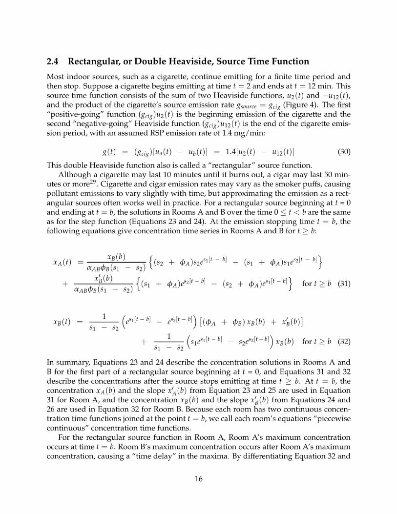
Figure 4: Rectangular source function for representing an indoor source that has zeroemissions of RSP for time t < 2 min and constant emission rate g(t) = gsource = 1.4mg/min for time 2 ≤ t < 12 min, followed by a zero emission rate for time t ≥ 12. Thisexample might represent the fine particle source emission raet for a filter cigarette smokedfor 10 min, showing the positive-going and negative-going Heaviside functions used tocreate a rectangular soruce function

15

2.4 Rectangular, or Double Heaviside, Source Time Function

Most indoor sources, such as a cigarette, continue emitting for a finite time period andthen stop. Suppose a cigarette begins emitting at time t = 2 and ends at t = 12 min. Thissource time function consists of the sum of two Heaviside functions, u2(t) and −u12(t),and the product of the cigarette’s source emission rate gsource = gcig (Figure 4). The first“positive-going” function (gcig)u2(t) is the beginning emission of the cigarette and thesecond “negative-going” Heaviside function (gcig)u12(t) is the end of the cigarette emis-sion period, with an assumed RSP emission rate of 1.4 mg/min:

g(t) = (gcig)[ua(t) − ub(t)] = 1.4[u2(t) − u12(t)] (30)

This double Heaviside function also is called a “rectangular” source function.Although a cigarette may last 10 minutes until it burns out, a cigar may last 50 min-

utes or more29. Cigarette and cigar emission rates may vary as the smoker puffs, causingpollutant emissions to vary slightly with time, but approximating the emission as a rect-angular sources often works well in practice. For a rectangular source beginning at t = 0and ending at t = b, the solutions in Rooms A and B over the time 0 ≤ t < b are the sameas for the step function (Equations 23 and 24). At the emission stopping time t = b, thefollowing equations give concentration time series in Rooms A and B for t ≥ b:

xA(t) =xB(b)

αABφB(s1 − s2)

{

(s2 + φA)s2es1[t − b] − (s1 + φA)s1es2[t − b]}

+x′B(b)

αABφB(s1 − s2)

{

(s1 + φA)es2[t − b] − (s2 + φA)es1[t − b]}

for t ≥ b (31)

xB(t) =1

s1 − s2

(

es1[t − b] − es2[t − b])

[

(φA + φB) xB(b) + x′B(b)]

+1

s1 − s2

(

s1es1[t − b] − s2es2[t− b])

xB(b) for t ≥ b (32)

In summary, Equations 23 and 24 describe the concentration solutions in Rooms A andB for the first part of a rectangular source beginning at t = 0, and Equations 31 and 32describe the concentrations after the source stops emitting at time t ≥ b. At t = b, theconcentration xA(b) and the slope x′A(b) from Equation 23 and 25 are used in Equation31 for Room A, and the concentration xB(b) and the slope x′B(b) from Equations 24 and26 are used in Equation 32 for Room B. Because each room has two continuous concen-tration time functions joined at the point t = b, we call each room’s equations “piecewisecontinuous” concentration time functions.

For the rectangular source function in Room A, Room A’s maximum concentrationoccurs at time t = b. Room B’s maximum concentration occurs after Room A’s maximumconcentration, causing a “time delay” in the maxima. By differentiating Equation 32 and

16

setting the derivative to zero, we obtain a useful expression for the time of the maximumconcentration tmax in Room B:

tmax =1

s1 − s2ln

(

F1s2 + F2s22

F1s1 + F2s21

)

+ b (33)

where F1 = (φA + φB)xB(b) + x′B(b) and F2 = xB(b). Substituting Room B’smaximum concentration time tmax from Equation 33 into Equation 32 gives the predictedvalue of the maximum concentration in Room B.

We illustrate the characteristic shapes of these two compartment solutions for a rectan-gular source by an example in which a cigar emits carbon monoxide (CO) in the kitchen ofa home (Room A), and the concentration is predicted for the adjacent living room (RoomB) using Equations 23, 24, 31, and 32 (Figure 5). In this example, we assume a cigar RoomA and emits CO at a rate of 70.6 mg/min (70,600 µg/min) and burns uniformly for 15min. The door between Room A and Room B is open only a few inches, restricting theair flow between the kitchen and living room, thus causing the rooms to behave as twocompartments. This example of a cigar as a rectangular source time function uses thefollowing values for the 6 physical parameters: kitchen and living room volumes vA = 34m3 and vB = 36 m3; air change rates φA = 4.65 air changes per hour (ach) and φB = 4.17ach; and interzonal flow factors αAB = 0.614 and αBA = 0.976. These parameter values aresimilar to those obtained using experiments in a house as described later in this paper.

At time t = 0, Figure 5 shows the concentration in Room A in this example risingsharply, with a much more gradual concentration increase in Room B. In Room A, thepredicted maximum concentration occurs at time t = 15 min, the ending time of the cigaremissions. In Room B, the predicted maximum concentration occurs at time t = 26.96 minusing Equation 33, or 11.96 min after the maximum concentration in Room A, illustratingthe time delay of the maximum in the second room. Later in this paper, we comparethe predicted two compartment solutions for a rectangular source with the experimentalmeasurement results for a cigar smoked in the kitchen, living room, and bedroom of areal home.

2.5 Single-Compartment Illustration

The familiar solutions for step and rectangular sources in a single compartment also canbe obtained by Laplace transforms, and the approach is illustrated here briefly. Equation13 for the two compartment model can be converted into a single-compartment modelfor Room A by eliminating the interzonal flow between Room A and Room B by settingwBA = 0 and αBA = 0:

1

φ A

dxA(t)

dt+ xA(t) =

1

wOAgA(t) (34)

Following the rules for solving differential equations by Laplace transforms (AppendixB) and solving for the Laplace transform XA(s) of Room A’s concentration, where GA(s)

17

Figure 5: Example showing theoretical solutions to the two-compartment indoor modelfor a rectangular time series source in Room A, the kitchen. The source ends at time b =15 min, and the analytical solution in each room consists of the difference between twopiecewise-exponential functions. The eigenvalues for the solutions in this example are s1

= 0.9924 h−1 and s2 = -7.827 h−1.

18

represents the Laplace transform of the emission rate gA(t) as a function of time givesthe following general Laplace transform solution for the single-compartment model withinitial conditions xA(0):

L{xA(t)} = XA(s) =φA

wA

GA(s)

s + φA+

xA(0)

s + φA(35)

For a step source function with a constant emission rate gsource beginning at t = 0, wesubstitute GA(s) = 1/s as before:

XA(s) =φA

(s + φA)wOAG(s) +

xA(0)

s + φA=

φA

wA

gsource

s(s + φOA)+

xA(0)

s + φA(36)

Because no prior indoor sources are present, the initial condition is xA(0) = 0 and thefar right-hand term in Equation 36 disappears. The remaining terms in Equation 36 areexpanded by partial fractions:

XA(s) =gsourceφA

s(s + φA)wOA=

gsource

swOA−

gsource

(s + φA)wOA(37)

The right-hand side of Equation 37 contains the same two Laplace transforms derivedin Appendix A with scaling factor gsource/wOA. The term containing 1/s is the Laplacetransform of the Heaviside function and the term containing 1/(s + φA) is the Laplacetransform of an exponential function with decay parameter α = φA. Using the relation-ships in Appendix A is equivalent to taking the “inverse Laplace transform” of Equation37 by inspection:

L−1{XA(s)} = xA(t) =gsource

wOAu0(t) −

gsource

wOAe−φAtu0(t) =

gsource

wOA(1 − e−φAt)u0(t)

(38)This familiar indoor solution usually is written without its Heaviside notation:

g(t) =gsource

wOA(1 − e−φAt) for t ≥ 0 (39)

Equation 39 has been used in research on ETS sources to characterize the indoor con-centrations of CO and particulate matter measured for a cigar in a tavern16 and a home.29

This model agreed well with measurements of CO and particles from cigarettes in a cham-ber and an automobile during the period in which the cigarette was burning.9

For a rectangular source of a nonreactive pollutant without major sinks that startsemitting at t = 0 and ends at time t = b, the parameter φA is the air exchange rate, oftendenoted in the literature as “a” and expressed in air changes per hour (ach or hours−1).Equation 39 can be written using another useful parameter, the residence time τ = 1/φA,or the amount of time required for one full room volume vA of air to be replaced:

xA(t) =gsource

wOA(1 − e−t/τ) for 0 ≤ t < b (40)

19

For b ≤ t, the concentration decays exponentially decays with time:

xA(t) =gsource

wOA(1 − e−b/τ)e(t − b)/τ = xA(b)e(t − b)/τ for b ≤ t (41)

The maximum concentration xA(max) occurs at the exact time t = b when the emissionsource ends:

xA(max) = xA(b) =gsource

wOA(1 − e−b/τ) (42)

Representing e−b/τ in Equation 42 as a Taylor expansion, and omitting terms raised to apower of 2 and higher gives a useful approximation for the case when the source durationb that is small compared with the residence time τ :

xA(max) =gsource

wAO

{

1 − 1 +b

τ−

1

2!

(

b

τ

)2

+1

3!

(

b

τ

)3

− ...

}

∼=(gsource)b

wOAτ

(43)For any source emitting at a constant rate gsource over a time duration b, the total massemissions generated will be msource = (gsource)b, and we can therefore substitute the sourcestrength msource for the product shown in the numerator in Equation 43. SubstitutingwAO = wOA = φAvA = vA/τ from Equation 7 for a single compartment (where wAB =wBA = 0) into the denominator in Equation 43 yields a useful practical result:

xA(max) ∼=msource

(vA/τ)τ=

msource

vA(44)

Thus, if b << τ for the single-compartment case, then the maximum concentrationin the room is approximately equal to the mass emitted msource divided by the volume ofthe room vA. This result is like imagining the mass emitted by the source to be uniformlydistributed in the air volume vA at or near the initial time t = 0, giving a predicted max-imum concentration (msoruce)/vA for a single compartment that decays exponentially fort > 0 at decay rate φA. Interestingly, the two compartment model in Equation 16 with animpulse source also yields the same initial concentration xA(max) = (msoruce)/vA at t = 0in Room A as in Equation 44.

This approximation has a practical application in both one- and two compartmentindoor air quality experiments. If the source emits for a short time period relative tothe air residence time of the room, and if its maximum concentration xA(max) can bedetermined by experiment, then the source strength can be calculated approximately asthe product of the room’s volume vA and the observed maximum concentration xA(max):

msource∼= vA · xA(max) (45)

3 Model Evaluation: Experiments in a Home

To evaluate how well compartmental indoor air models predict the time series of concen-trations for a cigarette smoked in a real home, we conducted more than 40 experiments

20

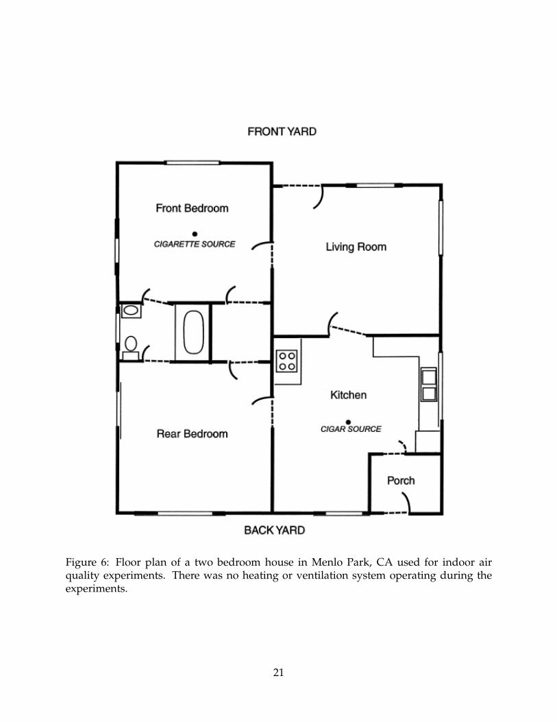
Figure 6: Floor plan of a two bedroom house in Menlo Park, CA used for indoor airquality experiments. There was no heating or ventilation system operating during theexperiments.

21

in a detached single-story, two-bedroom house with outside dimensions of 28 ft by 24ft, or 672 ft2 (62.5 m2) on Partridge Ave. in Menlo Park, CA (Figure 6). The house wasawaiting a new tenant and was not occupied, and we varied the locations of the monitorsand the door and window positions in a variety of configurations. The sources tested in-cluded Marlboro regular filter cigarettes, University of Kentucky 2R1 research cigarettes,and cigars. The Kentucky 2R1 cigarettes are standardized for research and are strongerthan commercially available cigarettes.

Selected results from these experiments were used to: (1) study the spatial variationof CO concentrations inside a single room of the residence (the bedroom), verifying thewell-mixed assumption, and calculate a cigarette mass emission rate; (2) observe howpollutant concentrations (RSP, PAH, CO) vary in two connected rooms of the residence(bedroom and living room); and (3) evaluate the equations developed in the previoussection for predicting CO concentrations observed in a pair of rooms – the kitchen andliving room.

3.1 Spatial Variation Within a Bedroom

An important assumption of the mass balance model (Equations 3 and 4) is that, for anytime t, the room is sufficiently well-mixed to give nearly the same concentration at alllocations. To evaluate this assumption, we made measurements at three widely spacedlocations in the 907.5 ft3 (25.7 m3) bedroom of this house1: (1) near the floor in the cornerof the room; (2) on a short step ladder 36" high in the center of the room; and (3) on a tallladder 8.5" from the ceiling (Figure 7). CO concentrations were measured using a LanganL15 CO Personal Exposure Measurer31 (Langan Products, San Francisco, CA). Each COsensor was connected by a wire to a DataBearTM data logger which logged the data at30-second intervals. For each CO sensor, a precision electronic operational amplifier mul-tiplied the signal by 10.0 to increase the numerical resolution, and concentrations weremeasured at high sensitivity31 and reported in parts-per-ten-million (pptm). Note that 10pptm is 1 ppm CO.

Over a period of 16 hours, three Marlboro regular filter cigarettes were smoked in thecenter of the bedroom at a 36" height with the doors closed and with one window partlyopen but covered with a shade. The first cigarette was smoked just after noon (12:46:30pm) and lasted for 6 minutes and 30 seconds; the exponential decay of the CO concentra-tions from this cigarette was quite similar for all three locations and lasted approximately4.25 hours until just before 5:00 pm (Figure 8). The second cigarette began approximatelyat 5:00 pm and lasted for 7 minutes and 16 seconds; it generated an exponential decaycurve at each of the three locations, although the concentration at the corner floor waslower than the concentration time series at the center of the room or at the ceiling. Finally,a third Marlboro cigarette was smoked at 9:56 pm for 9-1/2 minutes, and its exponentialdecay was observed until 3:49 am.. The air exchange rate was determined by subtract-ing the background concentration and taking the logarithms; the slope of the resulting

1These data have been previously analyzed by Klepeis (1999).17

22

Figure 7: Location of monitor positions in the bedroom (v = 25.7 m3) of the four-roomhouse in Menlo Park, CA in which experiments were conducted to determine the spatialvariation of indoor concentrations caused by smoking a cigarette.

23

Figure 8: Carbon monoxide (CO) concentrations measured at three locations in a 25.7m3 bedroom over a 16-hour period during which three Marlboro regular filter cigaretteswere smoked. See Figure 7 for a sketch of the room setup. The close agreement betweenmeasurements at all the three locations during the three experiments helps support the as-sumption of a spatially uniform concentration in the room, i.e., the room is “well-mixed”.

24

straight line yielded approximately the same ventilatory air exchange rate of φ = 1.2 airchanges per hour (ach) at all locations for this experiment.

Table 1: Average CO Concentration (pptm) Measured in the Bedroom at Three Locationsafter Smoking of Three Successive Marlboro Regular Filter Cigarettes

Experiment No. Corner Floor Center ofRoom

Top of Ladder Mean

1 5.62 6.81 5.90 6.112 5.18 6.30 5.61 5.703 4.19 5.16 3.88 4.41

Mean 5.00 6.09 5.13 5.41

The CO concentration time series, when averaged over each smoking episode, rangedfrom 3.88 pptm to 5.9 pptm, with an average for all episodes of 5.4 pptm (Table 1). Thecenter of the room averaged about 1-1.2 pptm (21-23%) higher than the corner floor andabout 0.7-1.3 pptm (19-33%) higher than the ceiling. One would expect a higher averageconcentration in the center, because the cigarette was smoked there within 12" of the COmonitor. It is unlikely that a person would spend several hours either at the two extremelocations – the corner floor or the ceiling – and the concentrations observed probablywould differ by less than the 19-33% from the mean. The average exposure of a personinside the room probably would be closer to the overall mean of 5.4 pptm, because theywould move around the room.

Baughman et al.15 studied a chamber with 40 sampling points to determine how rapidlythe concentrations at different points converge, and Mage and Ott16, in reviewing theirresearch, suggest three different time phases for an indoor source: an “alpha-period”in which the source is emitting and the concentrations vary spatially, a “beta-period”in which the source is off but the room is not yet well- mixed, and a “gamma-period” inwhich the coefficient of variation (i.e., the ratio of the standard deviation to the mean) acrossall monitoring points in the room is less than 0.10, and the room is judged to be “well-mixed.” There were too few monitoring locations in our bedroom experiment to computethe coefficient of variation, but Table 1 shows that the concentration time series patternafter the cigarettes end is similar at the three locations. For a cigarette, the alpha-periodis short relative to the other periods.

To estimate the cigarette mass emission rate, consider a previously published cigarette

smoking time series model,9 which expresses the average concentration xA(T) over time T

as a function of the average source strength gA(T), the instantaneous concentration x(T),the volume vA, and the air exchange rate φA:

gA(T)

φAvA− xA(T) =

xA(T)

TφA(46)

At the end of the exponential decay period, we assume xA(T) ∼= 0 so that

25

gA(T)

φAvA

∼= xA(T) (47)

The product of the average source emissions and the time T gives the total emissions mcig,so multiplying both sides of Equation 47 by TφAvA gives:

mcig = [gA(T)]T = [ x(T)]TφAvA (48)

Substituting the values of 5.41 pptm, φA = 1.2 air changes per hour (ach), vA = 25.7 m3,and the average experiment duration of 4.25 hours, we can compute the total source emis-sions for the cigarette experiment in the bedroom:

mcig = (0.541 ppm)

(

1.145mg

m3-ppm

)(

1.2air change

hr

)

(4.25 hr)

(

25.7m3

air change

)

= 81.2 mg (49)

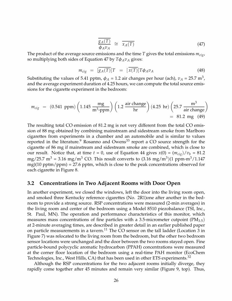
The resulting total CO emission of 81.2 mg is not very different from the total CO emis-sion of 88 mg obtained by combining mainstream and sidestream smoke from Marlborocigarettes from experiments in a chamber and an automobile and is similar to valuesreported in the literature.9 Rosanno and Owens33 report a CO source strength for thecigarette of 86 mg if mainstream and sidestream smoke are combined, which is close toour result. Notice that, at time t = 0, use of Equation 44 gives x(0) = (mcig)/vb = 81.2

mg/25.7 m3 = 3.16 mg/m3 CO. This result converts to (3.16 mg/m3)(1 ppm-m3/1.147mg)(10 pptm/ppm) = 27.6 pptm, which is close to the peak concentrations observed foreach cigarette in Figure 8.

3.2 Concentrations in Two Adjacent Rooms with Door Open

In another experiment, we closed the windows, left the door into the living room open,and smoked three Kentucky reference cigarettes (No. 2R1)one after another in the bed-room to provide a strong source. RSP concentrations were measured (2-min averages) inthe living room and center of the bedroom using a Model 8510 piezobalance (TSI, Inc.,St. Paul, MN). The operation and performance characteristics of this monitor, whichmeasures mass concentrations of fine particles with a 3.5-micrometer cutpoint (PM3.5)at 2-minute averaging times, are described in greater detail in an earlier published paperon particle measurements in a tavern.11 The CO sensor on the tall ladder (Location 3 inFigure 7) was relocated to the living room from the bedroom, but the other two bedroomsensor locations were unchanged and the door between the two rooms stayed open. Fineparticle-bound polycyclic aromatic hydrocarbon (PPAH) concentrations were measuredat the corner floor location of the bedroom using a real-time PAH monitor (EcoChemTechnologies, Inc., West Hills, CA) that has been used in other ETS experiments.32

Although the RSP concentrations for the two adjacent rooms initially diverge, theyrapidly come together after 45 minutes and remain very similar (Figure 9, top). Thus,

26

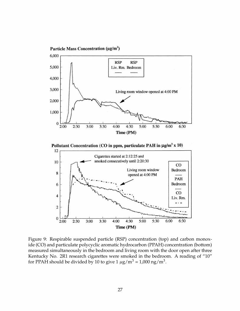
Figure 9: Respirable suspended particle (RSP) concentration (top) and carbon monox-ide (CO) and particulate polycyclic aromatic hydrocarbon (PPAH) concentration (bottom)measured simultaneously in the bedroom and living room with the door open after threeKentucky No. 2R1 research cigarettes were smoked in the bedroom. A reading of “10”for PPAH should be divided by 10 to give 1 µg/m3 = 1,000 ng/m3.

27

with the door between the bedroom and living room wide open, the two adjacent roomsbehave almost as a single compartment.

The RSP concentrations caused by the three Kentucky research cigarettes were ex-tremely high, reaching a momentary peak concentration of 5,500 µg/m3 in the bedroom.Indeed, the levels were so high that the three investigators found it necessary to open aliving room window at 4:00 pm, and the effect of opening this window in changing theair exchange rate is evident (Figure 9, bottom). Unlike CO, both RSP and particulate PAHare deposited on surfaces, and PAH therefore shows a more rapid decay than CO in thebedroom. It should be noted that the Kentucky No. 2R1 research cigarettes have higherparticulate emissions than ordinary retail cigarettes do.

3.3 Concentrations in Adjacent Rooms with Doors Almost Closed

To examine the relationships among the time series in several rooms, a cigar was smokedin the kitchen to provide a strong CO source, and the resulting CO concentrations weremeasured in the kitchen, living room, and bedroom. Long coaxial wire cables were ex-tended into each room with Langan L15 CO sensors attached at the end, and CO concen-trations on all three channels were logged using a DataBearTM data logger.29 As before,precision operational amplifiers multiplied the voltages by 10 to increase the sensitivity.31

The kitchen-to-living room door was open 3", and its position was locked in place bymasking tape. The living room-to-bedroom door was closed, and all windows in the liv-ing room and bedroom were closed. The other doors to nearby rooms were closed withtape attached around all the doors, leaving only three rooms through which CO couldreadily move.

The concentrations observed in two of the three rooms after a cigar was smoked inthe kitchen for 15 min (Figure 10) have the same general shapes as predicted by the twocompartment model in Figure 5 with a source in Room A (kitchen) and the concentrationobserved in Room B (living room). More pollutant transfer occurs if the door is open wide(Figure 9) or open a crack (3" for the kitchen door in Figure 10) than if the door is closedentirely (bedroom concentration in Figure 10), because the closed door acts as a barrierto movement of air. Except for the closed bedroom door, the doors to all the other roomsof the house were sealed tightly, so most of the air and pollutant flow occurs in the twocompartments represented by the kitchen and living room. Because of the importance ofthe door position and its effectiveness in shielding occupants of the home from ETS, itappears that additional research is needed to determine the effect of the door positionsand window positions on the interzonal pollutant movement in real homes.

To apply the two compartment model’s analytical solutions for rectangular source in-put, we must determine the values of all the parameters of the two compartment model.The volumes vA and vB are determined from physical measurement of the dimensionsof the rooms, but we still require the interzonal flow rate parameters αAB and αBA, theair change rates φA and φB, and the source strength msource. To find these values, weused a grid search method to find values of the 5 unknown parameters that yielded theminimum error. Values leading to negative flow rates were discarded. The error is de-

28

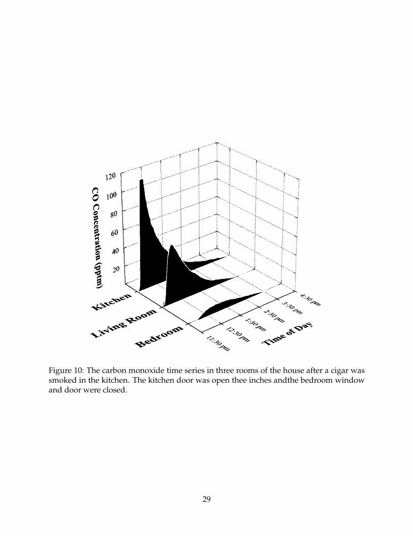
Figure 10: The carbon monoxide time series in three rooms of the house after a cigar wassmoked in the kitchen. The kitchen door was open thee inches andthe bedroom windowand door were closed.

29

Figure 11: Example of a three-dimensional plot of the optimization error surface whentwo parameters, Room A’s air exchange rate φA and the interzonal flow factor αBA re-flecting the proportion of air flow that Room A receives from Room B, are varied over awide range. This error surface is the mean absolute deviation between the predicted andobserved concentration time series, and a minimum occurs at φA = 4 h−1 and αBA = 0.95,the lowest point of a shallow channel.

fined as the mean absolute deviation between the model-predicted concentration curveand the measured concentration curve. In the grid search method, the parameter valuesbegin with an initial starting point and then small increments are subtracted or addediteratively to each parameter to reduce the error. At the end of a number of computeriterations, the final values of the parameters are those giving the smallest error. Althoughit is not possible to plot the error surface in 5 dimensions, we can give an example of theerror surface plotted in 3 dimensions as a function of the air exchange rate in the kitchenφA and the proportion of the air flow that Room A receives from Room B, αBA (Figure11). This graph shows a minimum pathway (or channel) in the error surfaceas well asflat areas with high uncertainty in the estimated parameter values (i.e., the values corre-sponding to the minimum error point). In the flat regions, there is uncertainty about thevalues of the parameters. For this particular surface, a fairly narrow channel exists frommoderate values of φA and αBA to their optimum values of 4 hr−1 and 0.95, respectively.

Figure 12 shows the two compartment model fit to the complete CO time series in thekitchen and the living room of the small residence (Figure 6), with a cigar smoked for 15min in the kitchen. This fit represents a minimum value in the error surface. The gridsearch minimization approach gave the following values of the parameters: air changerates of φA = 4 hr−1 in the kitchen and φB = 4.6 hr−1 in the living room; interzonal flowratios of αBA = 0.95 for the kitchen and αAB = 0.62 for the living room, and gsource = 60mg/min for 15 min, giving a source strength of msource = (60 mg/min)(15 min) = 900 mg,which is comparable to the CO source strengths observed in other cigar experiments.29

30

Figure 12: Comparison of carbon monoxide (CO) concentration predicted by the two-compartment model with CO concentration measured in the kitchen and living room ofthe house in Menlo Park, CA after a cigar was smoked for 15 min in the kitchen. Thevalues of the five parameters were obtained by a grid search optimization method. Theresulting air exchange rates for the kitchen and living room were φA = 4 h−1 and φB =4.6 h−1, respectively. The interzonal flow percentages were 95% for the kitchen, i.e., theproportion of air that the kitchen receives from the living room is 0.95, and 62% for theliving room, i.e., the proportion of air that the living room receives from the kitchen is0.62. The cigar’s soruce emission rate was found to be gsource=60 mg/min, which issimilar to the CO emission rates for cigars reported elsewhere.29

31

The two compartment model fits the experimental data reasonably well throughout theduration of the experiment, except for the beginning of the source room time series whereit appears that nonuniform mixing in the kitchen (Room A) during the alpha-periodcaused a decreased concentration. The living room concentration time series (Room B)fits very well, even at the very beginning. The two rooms obviously behave as two com-partments despite relatively high air change rates (4-6 hr−1) and fairly high interzonalflow rate (95% of the air entering the kitchen is from the living room and 62% of the airentering the living room is from the kitchen).

Calculating the overall air change rate with the outdoor air for the two rooms com-bined shows that it is much lower than the individual room air change rates of φA = 4 hr−1

and φB = 4.6 hr−1. For example, the total volumetric air flow in Room A is wA = vAφA =(34 m3)(4 hr−1) = 136 m3/hr, and the total volumetric air flow in Room B is wB = vBφB =(36 m3)(4.6 hr−1) = 165.6 m3/hr. Using the formulas for αAB and αBA in Equations 9 and11, we calculate the interzonal flow rates as wAB = (wAB + wOB)αAB = wBαAB = (165.6m3)(0.62) = 102.7 m3/hr and wBA = (wBA + wOA)αBA = wAαBA = (136 m3)(0.95) = 129.2m3/hr. As discussed in the text after Equations 7−12, the total air flow for rooms A and Bwith the outdoors and other rooms, minus internal flows between them is: w = wA + wB

– (wBA + wAB) = 136 + 165.6 – (102.7 + 129.2) = 301.6 – 221.9 = 69.7 m3/hr. Therefore, theoverall air change rate for the two rooms is φ = w/(vA + vB) = 69.7/(34 + 36) = 0.995hr−1. This result is close to 1 air change per hour, typical of the air change rates for asmall California residence with the external doors and windows closed. Thus, the higherair change rates for the individual rooms reflect the more rapid air flow occurring be-tween the kitchen and the living room when the door between these two adjacent roomsis open 3” (7.6 cm).

These results illustrate that one can determine all the parameters for the two compart-ment model in a single experiment, although the relatively flat error surface in Figure 11suggests that a range of parameter values around the optimal values would cause almostas good a fit to the data as the optimal values. One reason that compartmental indoorair quality experiments often use two or more tracer gases instead of the single gas usedhere is an attempt to reduce uncertainty in the parameter values. However, the flat errorsurface has a practical advantage: slight errors in the parameter values do not impair theexcellent fit of the predicted time series to the measured concentration time series in bothrooms.

4 Summary and Conclusions

In this paper, we use Laplace transforms to represent indoor sources of air pollution withemission rates that begin and end at specific times, and solve the basic indoor differentialequations algebraically for one and two compartments for impulse, step, and rectangularsource time functions. We apply the solutions to a real house where the predicted andcontinuously measured concentrations are compared in several rooms. The predictedtime series showed good agreement with the continuous measurements measured in this

32

home. Our approach yielded analytical expressions for the slopes, maxima, and pointsof inflection of the predicted curves that may be of practical use in other indoor air qual-ity studies. These analytical expressions are an alternative to Runge-Kutta methods thattake tiny iterative steps on a computer using discrete versions of the same differentialequations.

Although this paper presents analytical solutions for the impulse, step, and rectan-gular source functions, there are other common indoor source functions for which thesegeneral methods are suitable. These methods, illustrated here for ETS sources, can beapplied to any indoor source whose Laplace transform can be found.

Because the duration of a cigarette often is brief relative a house’s residence time τ(i.e.,the reciprocal of the air change rate) the cigarette source sometimes can be represented byan impulse function instead of a rectangular source function. With this approximation,the total amount of pollutant emitted by the cigarette, or its total mass source strengthmcig, is the product of the volume of the compartment vand the estimated maximumconcentration. This result agrees with common sense: if a pollutant mcig suddenly dis-persed uniformly over a single compartment’s mixing volume v, then the resulting initialmaximum concentration will be approximately equal to the mass released divided by thevolume, or (mcig)/v.

For the single-compartment case with an impulse, step, or rectangular source timefunction, the analytical solution is a single exponential function of time. For the two com-partment case, the analytical solution is the difference between two exponential functionsof time. Analytical solutions have been derived for the maxima and can be applied usinga hand calculator. The two eigenvalues for the two compartment solutions, which dependon the physical volume, air change rates, and interzonal flow factors of the rooms, deter-mine the times of occurrence of the maximum concentrations and points of inflection forthe predicted concentration time series.

In our experiments using continuous measurements in three rooms of a small, de-tached home, we found that two rooms with an open door between them behaved asa single compartment. In contrast, two adjacent rooms with the door tightly closed oropened slightly (for example, 3" or less) behaved as two separate compartments. Our ex-periments also showed that the position of the doors and windows had a large effect onthe indoor concentrations in different rooms. Our results suggest that a smoker indoorsmay be able to confine the ETS generated in a particular part of the home by closing thedoors and opening windows in the room in which the smoking takes place, thereby re-ducing the ETS exposure of other residents. More research is needed on the effectivenessof this indoor “isolation" effect.

Howard-Reed et al.18 studied the effect of window positions on the air change rates oftwo homes, and it appears that future research should focus systematically on the effectof other similar factors in the home. These factors include opening and closing inter-nal doors, the compartmental effect of hallways, the effect of fans and ventilation sys-tems, and other physical and human activities that may influence indoor pollutant con-centrations. The increasing use of real-time measurement methods in indoor residentialsettings36 promises to provide important new insights into the factors affecting indoor air

33

and human exposure to environmental pollutants in the home. Indoor predictions basedon validated models and indoor source strengths allow the findings from one home to beextended and generalized to other homes.

Acknowledgments

This research was supported in part by the Cigarette and Tobacco Surtax Fund of the Stateof California through the Tobacco-Related Disease Research Program of the University ofCalifornia (Grant No. 6RT-0118). This work was also supported by the U.S. Environmen-tal Protection Agency (EPA) National Exposure Research Laboratory through InteragencyAgreement DW-988-38190-01-0 with the U.S. Department of Energy (DOE) under Con-tract Grant No. DE-AC03-76SF00098 at Lawrence Berkeley National Laboratory (LBNL)and through an LBNL subcontract to Stanford University.

References

1. Klepeis, N.E., Nelson, W.C., Ott, .W.R., Robinson, J.P., Tsang, A.M., Switzer, P., Be-har, J.V., Hern, S.C., Engelmann, W.H. (2001) “The National Human Activity PatternSurvey (NHAPS): A Resource for Assessing Exposure to Environmental Pollutants,”Journal of Exposure Analysis and Environmental Epidemiology, Vol 11(3), pp. 231-252.

2. Wadden, R.A. and Scheff, P.A. Indoor Air Pollution: Characterization, Prediction, andControl, John Wiley & Sons (1983).

3. Ott, W.R. (1999) “Mathematical Models for Predicting Indoor Air Quality from Smok-ing Activity,” Environmental Health Perspectives, Vol. 107, Supplement 2, May 1999,pp. 375-381.

4. McKone, T.E. “Household Exposure Models,” Toxicology Letters, Vol. 49. pp. 321-339(1989).

5. Wilkes, C.R., Small, M.J., Andelman, J.B., Giardino, N.J., and Marshall, J. “InhalationExposure Model for Volatile Chemicals from Indoor Uses of Water,” Atmos. Environ.,Vol. 26A, No. 12, pp. 2227-2236 (1992).

6. Axley, J.W., and Lorenzetti, D. “IAQ Modeling Using STELLATM: A Tutorial In-troduction,” Building Technology Program, Massachusetts Institute of Technology,(Fall 1991).

7. Sparks, L.E., Tichenor, B.A., White, J. B., Chang, J. and Jackson, M.D. “Verifica-tion and Uses of the Environmental Protection Agency (EPA) Indoor Air QualityModel,” Paper No. 91-62.12 presented at the 84th Annual Meeting of the Air andWaste Management Association, British Columbia, June 16-21 (1991).

34

8. Nagda, N., ed., Modeling of Indoor Air Quality and Exposure, ASTM STP 1205, Ameri-can Society for Testing and Materials, West Conshohocken, PA (1993).

9. Ott, W., Langan, L., and Switzer, P. “A Time Series Model for Cigarette SmokingActivity Patterns: Model Validation for Carbon Monoxide and Respirable Particlesin a Chamber and an Automobile,” J. Expos. Anal. & Environ. Epidemiology, Vol. 2,Suppl. 2, pp. 175- 200 (1992).

10. Klepeis, N.E., Ott, W.R. and Switzer, P. “A Multiple-Smoker Model for PredictingIndoor Air Quality in Public Lounges,” Environ. Sci. & Technol., Vol 30, No. 9, pp.2813-2820 (1996).

11. Ott, W., Switzer, P. and Robinson, J. “Particle Concentrations Inside a Tavern Beforeand After Prohibition of Smoking: Evaluating the Performance of an Indoor AirQuality Model,” J. Air & Waste Manag. Assoc., Vol. 45, No. 12, pp. 2-16 (1996).

12. Miller, S.L., Leiserson, K., and Nazaroff, W.W., “Nonlinear Least-Squares Minimiza-tion Applied to Tracer Gas Decay for Determining Airflow Rates in a Two-ZoneBuilding,” Indoor Air, Vol. 7, pp. 64-75 (1997).

13. Miller, S.L. and Nazaroff, W.W., “Environmental Tobacco Smoke Particles in Multi-zone Indoor Environments,” Atmospheric Environment, Vol. 35, pp. 2053-2067 (2001).

14. Rogers, L.C. (1980) “Air Quality Levels in a Two-Zone Space,” ASHRAE Transac-tions, vol. 86, Part 2, pp. 92-98.

15. Baughman, A.V., Gadgil, A.J., and Nazaroff, W.W. “Mixing of a Point Source Pollu-tant by Natural Convection Flow Within a Room,” Indoor Air, Vol. 4, pp. 114-122(1994).

16. Mage, D.T., and Ott, W.R. “The Correction for Nonuniform Mixing in Indoor Mi-croenvironments,” in Tichenor, B.A., Characterizing Indoor Air Pollution and Re-lated Sink Effects, STP-1287, pp. 263-278, ASTM, West Conshohocken, PA (1996).

17. Klepeis, N.E., “Validity of the Uniform Mixing Assumption: Determining HumanExposure to Environmental Tobacco Smoke,” Environmental Health Perspectives, 1999.Vol. 107, pp. 357-363.

18. Howard-Reed, C., Wallace, L.A., and Ott, W.R., “The Effect of Opening Windows onAir Change Rates in Two Homes,” accepted for publication in the Journal of the Airand Waste Management Association 82:147-159 (2002).

19. Pandian, M., Behar, J., Ott, W., Wallace, L., Wilson, A.L., Colome, S. and Koontz, M.“Correcting Errors in the Nationwide Data Base of Residential Air Exchange Rates,”J. Expos. Anal. & Environ. Epidem. 8(4):577-586 (1998).

35

20. Dorf, R.C., and Bishop, R.H. “Introduction to Control Systems,” Addison-Wesley,Reading, MA (1996).

21. D’Azzo, J.J., Linear Control System Analysis and Design: Conventional and Modern,Fourth Edition, McGraw Hill (New York 1995).

22. D’Azzo. J. and Houpis, C.J. Feedback Control System Analysis and Synthesis, McGraw-Hill (New York 1966).

23. Franklin, G.F., Powell, J.D., and Emani-Naeini, A., Feedback Control of Dynamic Sys-tems, Third Edition, Addison-Wesley Publishing Co. (Reading, MA 1994).

24. Gujic’, Z., and M. Lelic’, Modern Control Systems Engineering, Prentice-Hall, London,(1996).

25. Nise, N.S., Control Systems Engineering, Second Edition, The Benjamin/CummingsPublishing Co. (Redwood City, CA 1995).

26. Blanchard, P., Devaney, R.L., and Hall, G.R. (1997) Differential Equations, Brooks/ColePublishing Co., Pacific Grove, CA.

27. Bugl, P. (1995) Differential Equations: Matrices and Models, Prentice Hall, EnglewoodCliffs, NJ.

28. Edwards, C.H., and Penney, D.E. (1996) Differential Equations and Boundary ValueProblems, Prentice Hall, Upper Saddle River, NJ.

29. Klepeis, N.E., Ott, W.R., and Repace, J.L.., “The Effect of Cigar Smoking on IndoorLevels of Carbon Monoxide and Particles,” Journal of Exposure Analysis and Environ-mental Epidemiology , Vol. 9, pp. 622-635 (1999).

30. Ott, W., and Switzer P. “Analytical Solutions to the two compartment Indoor Modelby Laplace Transforms,” Research Report, Department of Statistics, Sequoia Hall,Stanford, CA 94305 (2002).

31. Langan, L. “Portability in Measuring Exposure to Carbon Monoxide,” J Expos. Anal.and Environ. Epidemiology, Supplement 1, pp. 223-239 (1992).

32. Ott, W.R., Vreman, H.J., Switzer, P., and Stevenson, D.K. “Evaluation of Electro-chemical Monitors for Measuring Carbon Monoxide Concentrations in Indoor, In-Transit, and Outdoor Microenvironments,” in “Measurement of Toxic and RelatedAir Pollutants,” Proceedings of the U.S.EPA/A&WM International Symposium, Re-search Triangle Park, NC, Air and Waste Management Association, Pittsburgh, PA,VIP-50, pp. 172-177 (1995).

33. Rosanno, A.J. and Owens, D.F. “Design Procedures to Control Cigarette Smoke andOther Air Pollutants,” ASHRAE Transactions, Vol. 75, pp. 93-102 (1969).

36

34. Ott, W.R., Wilson, N.K., Klepeis, N.E., and Switzer, P. “Real-time Monitoring ofPolycyclic Aromatic Hydrocarbons and Respirable Suspended Particles from En-vironmental Tobacco Smoke in a Home,” in “Measurement of Toxic and Related AirPollutants,” Proceedings of the U.S.EPA/A&WM International Symposium, Durham,NC, EPA/600/R-94/136, Air and Waste Management Association, Pittsburgh, PA,VIP-39, pp. 887-892 (1994).

35. Wilson, N.K., Barbour, R.K., Chuang, J.C., and Mukund, R. “Evaluation of a Real-Time Monitor for Fine Particle-Bound PAH in Air,” Polycyclic Aromatic Compounds,Vol. 5, pp. 167-174 (1994).

36. Long, C.M., Suh, H.H., and Koutrakis, P. “Characterization of Indoor Particle SourcesUsing Continuous Mass and Size Monitors,” J. Air and Waste Management Associa-tion, Vol. 50, pp. 1236-1250 (July 2000).

A Laplace Transforms of the Source Time Functions in this

Paper

The general Laplace transform function X(s) of the function x(t) is defined by:

L{x(t)} = X(s) =

∞∫

0

x(t)e−stdt (50)

For the Heaviside function x(t) = ua(t), Laplace transform is derived as

L{ua(t)} =

∞∫

a

ua(t)e−stdt = limb→∞

b∫

a

ua(t)e−stdt

= limb→∞

ba

[

1

− se−st

]

= 0 −1

−se−at =

e−at

s(51)

If the Heaviside function is shifted to the origin, substituting t = 0 into Equation 51gives e0 = 1 for a Heaviside function that begins at t = 0:

L{u0(t)} =1

s(52)

For the exponential function x(t) = e−αt for t ≥ 0, where α is the decay parameter, theLaplace transform of a decaying exponential function is derived as

37

L{e−αt} =

∞∫

0

e−αte−stdt = limb→∞

b∫

0

e−(α + s)tdt

= limb→∞

b0

[

−1

α + se−(α + s)t

]

= 0 +1

α + se0 =

1

α + s(53)

B Laplace Approaches for Solving Differential Equations

Given a function x(t) with Laplace transform L{x}, the Laplace transform of dx/dt is

L

{

dx

dt

}

= sL{x} − x(0) (54)

L

{

d2x(t)

dt2

}

= sL{dx(t)

dt} − x′(0) = s[sL{x(t)} − x(0)] − x′(0)

= s2L{x(t)} − sx(0) − x′(0) (55)

38