analytical models of heat conduction in fractured...

$: Analytical models of heat conduction in fractured rocksmaeresearch.ucsd.edu/tartakovsky/Papers/ruiz-2014-analytical.pdf · JournalofGeophysicalResearch:SolidEarth RESEARCHARTICLE$
Journal of Geophysical Research: Solid Earth

RESEARCH ARTICLE10.1002/2012JB010016

Key Points:• Analytical models for heat transfer in

fracture networks are derived• Matrix diffusivity tensor is a key

parameter controlling fracturetemperature

• Classical models overestimatefracture temperature andtime-to-equilibrium

Correspondence to:D. M. Tartakovsky,[email protected]

Citation:Ruiz Martínez, Á., D. Roubinet, and D. M.Tartakovsky (2014), Analytical modelsof heat conduction in fracturedrocks, J. Geophys. Res. Solid Earth, 119,doi:10.1002/2012JB010016.

Received 29 DEC 2012

Accepted 11 DEC 2013

Accepted article online 16 DEC 2013

Analytical models of heat conduction in fractured rocksÁ. Ruiz Martínez𝟏, D. Roubinet𝟏, and D. M. Tartakovsky𝟏

1Department of Mechanical and Aerospace Engineering, University of California, San Diego, La Jolla, California, USA

Abstract Discrete fracture network models routinely rely on analytical solutions to estimate heat transferin fractured rocks. We develop analytical models for advective and conductive heat transfer in a fracturesurrounded by an infinite matrix. These models account for longitudinal and transverse diffusion in thematrix, a two-way coupling between heat transfer in the fracture and matrix, and an arbitrary configurationof heat sources. This is in contrast to the existing analytical solutions that restrict matrix conduction to thedirection perpendicular to the fracture. We demonstrate that longitudinal thermal diffusivity in the matrixis a critical parameter that determines the impact of local heat sources on fluid temperature in the fracture.By neglecting longitudinal conduction in the matrix, the classical models significantly overestimate bothfracture temperature and time-to-equilibrium. We also identify the fracture-matrix Péclet number, definedas the ratio of advection timescale in the fracture to diffusion timescale in the matrix, as a key parameterthat determines the efficiency of geothermal systems. Our analytical models provide an easy-to-use tool forparametric sensitivity analysis, benchmark studies, geothermal site evaluation, and parameter identification.

1. Introduction

Heat transfer in fractured rocks is a critical phenomenon that drives the performance of both enhancedgeothermal systems (wherein the heat transferred from hot dry rocks warms water circulating in fractures)[Willis-Richards et al., 1996; Gelet et al., 2012] and enhanced oil recovery (wherein oil viscosity is reduced byinjecting hot water or steam, thus increasing rock temperature) [Al-Hadhrami and Blunt, 2001]. Heat conduc-tion impacts the structural properties of ambient rocks by creating new or reopening existing microfractures[Wang et al., 1989; Lin, 2002] and/or modifying rock alteration patterns [Xu and Pruess, 2001]. Its negativeeffects are manifested in seismic activity induced by geothermal energy extraction [Gunasekera et al., 2003;Chen and Shearer, 2011] and in nuclear waste leakage due to heat generated by radioactive decay [Xiangand Zhang, 2012; Wang et al.,1981].

Heat transfer in fractured subsurface environments takes place in at least two distinct phases: fluid-filledfractures and ambient solid matrix. Existing analytical and semianalytical models of heat conduction infractured rocks consider single isolated fractures [Meyer, 2004] and networks of equally spaced horizontal[Bodvarsson and Tsang,1982] or vertical [Yang and Yeh, 2009; Gringarten et al., 1975] fractures. It is impor-tant to recognize that single-fracture representations are important not only in their own right but alsoas conceptual representations of mobile/immobile regions in natural fractured systems [Zhou et al., 2007].Such models are amenable to the same mathematical treatment as their counterparts developed for masstransport in discrete fracture networks. Examples of the latter include analytical [Tang et al., 1981], semiana-lytical [Roubinet et al., 2012; Sudicky and Frind, 1982], and numerical [Roubinet et al., 2010] models of solutetransport due to advection and diffusion in fractures and pure diffusion in the host matrix. A key differ-ence between heat and mass transfer in fractured environments is that heat readily diffuses through bothsolid and fluid phases, whereas solutes spread largely in the fluid phase. While potentially important [e.g.,Bataillé et al., 2006], investigation of variable-density flow and heat transport lies outside the scope of thepresent study.

Analytical solutions, such as those mentioned above, provide significant physical insight into these trans-port phenomena and act as an invaluable component in field-scale screening and management (decisionsupport) models. Yet they rely on a number of simplifying assumptions that might not be valid in a specificapplication. While these solutions routinely neglect longitudinal diffusion in the matrix, its impact on heatand mass transfer can be significant [Molson et al., 2007; Roubinet et al., 2012]. Likewise, longitudinal dif-fusion in the matrix (which is typically neglected in analytical models) is an important mechanism of heattransfer in a system of several fractures [Cheng et al., 2001; Baston and Kueper, 2009; Kolditz, 1995]. It can

RUIZ MARTíNEZ ET AL. ©2013. American Geophysical Union. All Rights Reserved. 1

http://publications.agu.org/journals/

http://onlinelibrary.wiley.com/journal/10.1002/(ISSN)2169-9356

http://dx.doi.org/10.1002/2012JB010016

http://dx.doi.org/10.1002/2012JB010016

Journal of Geophysical Research: Solid Earth 10.1002/2012JB010016

Figure 1. Single fracture embedded in an infinite matrix.

overestimate the thermal drawdown by up to 11% after 20 years of heat mining from HDRs in fracturedcrystalline rocks [Kolditz, 1995].

In the present study, we develop an analytical model of heat transfer in individual fractures, which accountsboth for longitudinal and transverse diffusion in the matrix and for longitudinal and transverse dispersionand diffusion in the fracture. Section 2 provides a mathematical formulation of the problem. Section 3 con-tains its general solution in the Fourier-Laplace space. This solution is inverted analytically under conditionsthat are typical of most geothermal reservoirs (section 3.2). We compare our analytical solutions with theirexisting counterparts in section 4 and demonstrate their physical and practical implications in section 5.Major conclusions from our study are summarized in section 6.

2. Problem Formulation

Consider fluid flow and heat transfer in a fracture with aperture 2b and infinite length that is embeddedin a homogeneous rock matrix with porosity 𝜙 (Figure 1). Following the standard practice in the field [e.g.,Kolditz, 1995; Cheng et al., 2001; Baston and Kueper, 2009; Xiang and Zhang, 2012], we assume the steadystate flow to be single phase, incompressible, and laminar; the gravity effects and density variation withtemperature to be negligible; and the fracture walls to be smooth and parallel to each other. Some of theseassumptions can be relaxed, as discussed in the concluding remarks in section 6. Since the problem is sym-metric about the plane z = 0, we restrict our analysis to the upper half of the computational domain, sothat the fracture is represented by Ωf = (x, z) ∶ −∞ < x < ∞, 0 ≤ z ≤ b and the matrix byΩm = (x, z) ∶ −∞ < x < ∞, b ≤ z < ∞. Fluid temperature in the fracture, T f (x, z, t), satisfies anadvection-dispersion equation

𝜕T f

𝜕t+ u

𝜕T f

𝜕x= Df

L

𝜕2T f

𝜕x2+ Df

T

𝜕2T f

𝜕z2+ f , 𝐱 ∈ Ωf (1)

where 𝐱 = (x, z)⊤ is the position vector, u is the fluid velocity, f (𝐱, t) is a source term, and DfL

and DfT

are thelongitudinal and transverse dispersion coefficients, respectively. For a fluid of density 𝜌f and heat capacity cf ,these are given by Df

L= 𝜆f

L∕𝛼f + Ef

L∕𝛼f and Df

T= 𝜆f

T∕𝛼f + Ef

T∕𝛼f , where 𝛼f = 𝜌f cf , 𝜆

fL

and 𝜆fT

are the longitudi-nal and transverse thermal conductivity coefficients, and Ef

Land Ef

Tthe longitudinal and transverse thermal

dispersion coefficients [Yang and Yeh, 2009].

The ambient matrix Ωm is assumed to be impervious to flow. The heat spreads throughout the matrix byconduction, so that temperature in the matrix, T m(𝐱, t), is governed by a diffusion equation

𝜕T m

𝜕t= Dm

L

𝜕2T m

𝜕x2+ Dm

T

𝜕2T m

𝜕z2, 𝐱 ∈ Ωm, (2)

where DmL= 𝜆e

L∕ce and Dm

T= 𝜆e

T∕ce are the longitudinal and transverse diffusion coefficients, ce is the effective

heat capacity of the matrix, and 𝜆eL

and 𝜆eT

the longitudinal and transverse thermal conductivity coefficientsin the matrix.

Let Ti(x, z) denote the initial temperature in the system. Then equations (1) and (2) are subject to initialconditions

T f (x, z, 0) = Ti(x, z), T m(x, z, 0) = Ti(x, z). (3)


http://dx.doi.org/10.1002/2012JB010016


Equation (1) is subject to boundary conditions

T f (±∞, z, t) = Ti,𝜕T f

𝜕z(x, 0, t) = 0, (4)

and equation (2) to boundary conditions

T m(±∞, z, t) = Ti, T m(x,∞, t) = Ti. (5)

At the fracture-matrix interface z = b, both the temperature and the heat flux are continuous, giving rise totwo interfacial conditions

T f = T m, 𝜙mDmT

𝜕T m

𝜕z= Df

T

𝜕T f

𝜕z≡ r, z = b, (6)

where 𝜙m = 𝜙 + (1 − 𝜙)𝜌scs∕(𝜌f cf ); 𝜌s and cs are the density and heat capacity of the solid phase, respec-tively; and r(x, t) is the (unknown) thermal flux between the fracture and matrix. Since the boundary valueproblems (BVPs) (1)–(6) are invariant under transformations T = T j − Ti (j = f ,m), we set, without loss ofgenerality, Ti = 0.

In what follows, we first develop general solutions of BVPs (1)–(6), which are applicable to a wide range ofsource functions f (𝐱, t). Then we proceed by analyzing these solutions in detail for f representing a pointinjection of heat at x = 0. This setting is relevant to both natural and forced convection. For example, itrepresents fluid injection through a well that intersects a fracture at x = 0. If the temperature of the injectedfluid is appreciably different from the initial temperature Ti of the host fluid, then this setup can be usedto characterize fractured rocks by collecting temperature logs at the well; Pehme et al. [2007, 2010] usedit to detect the presence of active fractures under natural groundwater flow conditions. Another exampledescribed by the model is an enhanced geothermal system, in which the fluid velocity u is induced by, e.g.,groundwater extraction at point x = xi > 0. If the fracture fluid is at the initial temperature Ti, the objective isto evaluate how the temperature of the fluid extracted at x = xi is modified by warmer/colder water injectedat x = 0 under forced flow conditions.

3. Analytical Solutions

The fracture BVP consists of (1), (3), (4) and the second condition in (6). The matrix BVP is composed of (2),(3), (5) and the second condition in (6). Let Gf (x, z; x′, z′; t − t′) and Gm(x, z; x′, z′; t − t′) denote the Green’sfunctions associated with the fracture and matrix BVPs, respectively. Their analytical expressions are given inAppendix A.

Our analytical models are first derived in the Fourier-Laplace (FL) space. For any suitable function A(x, t), wedefine its Laplace and Fourier transformations as

A(x, s) =

∞

∫0

A(x, t)e−stdt, (7a)

A(𝜉, s) = 1√2𝜋

∞

∫−∞

A(x, s)e−ix𝜉dx. (7b)

3.1. General Solution in Fourier-Laplace SpaceWe show in Appendix B that the FL transforms of the temperature in the fracture, T f (𝜉, z, s), and matrix,T m(𝜉, z, s), are given by

T f =√

2𝜋[

F1(𝜉, s)Δ (b; 𝜉; s)F2(𝜉, s) + 1∕𝛽

− Δ (z; 𝜉; s)]

(8)

and

T m = −√

2𝜋𝛽

exp

(−𝜓|z − b|√

DmT

)Δ (b; 𝜉; s)

F2(𝜉, s) + 1∕𝛽. (9)


http://dx.doi.org/10.1002/2012JB010016


Here Δ (z; 𝜉; s) = (z, 0; 𝜉; s) − (z, b; 𝜉; s), (z, z′; 𝜉; s) is the antiderivative of f Gf with respect to z′, 𝜓 =√Dm

L 𝜉2 + s, 𝛽 = 𝜙m

√Dm

T 𝜓 , and

F1 =Gf𝜉(s)

b+ 2

b

∞∑n=1

(−1)n cos(𝛼nz)Gf𝜉(s + 𝛼2

nD f

T) (10a)

F2 =Gf𝜉(s)

b+ 2

b

∞∑n=1

(−1)2nGf𝜉(s + 𝛼2

nD f

T) (10b)

where Gf𝜉(s) is given by (A4) and 𝛼n = n𝜋∕b.

The FL transform of the temperature distribution in the fracture-matrix system, (8) and (9), is free of any sim-plifying assumptions. It captures full (two-way) coupling of the fracture-matrix exchange and accounts forlongitudinal and transverse dispersion and diffusion in the fracture and matrix, respectively. It also enablesone to deal with arbitrary heat sources.

3.2. Explicit Models of Temperature in the FractureIn the case of complete transverse mixing (Df

T= ∞) and negligible longitudinal dispersion (Df

L= 0) in

the fracture, the general FL solutions (8) and (9) can be inverted analytically, yielding a closed-form expres-sion for the temperature distribution. These conditions are typical for fracture-matrix systems. Indeed, theimpact of longitudinal dispersion is limited to low velocities (≤ 10−7 m/s) [Tang et al., 1981], and transversedispersion is important only if Df

T< Dm

T[Roubinet et al., 2012].

Consider a continuous-in-time point source located at x = 0, such that f = T0u𝛿(x)(t), where T0 is thetemperature of the injected fluid (or the difference between the temperature of the injected fluid and itsinitial value Ti if the latter is not zero) and (⋅) is the Heaviside function. In the limit of Df

T→ ∞ and Df

L→ 0,

(8) reduces to

T f = 1√2𝜋s

T0u

𝛽∕b + s + u𝜉i. (11)

Let us define dimensionless ratio R, coefficient K , and critical time tmin as

R =𝜙m

√Dm

T DmL

ub, K =

𝜙m

2b

√Dm

T

DmL

, tmin = 104b2

𝜙2m

DmT

. (12)

Note that since√

DmT Dm

L is the geometric mean of the heat diffusivity in the matrix and u∕𝜙m is a scaledadvective velocity in the fracture, one can think of R as the inverse of a “fracture-matrix Péclet number” inthat it represents a ratio of advection timescale in the fracture to diffusion timescale in the matrix. We showin Appendix C that for R > 1, K > 1, and t > tmin, the inverse FL transformation of (11) yields

T f (x, t) ∼ −T0

2𝜋REi

(− 1

4t∗d

)+

T0

21

sgn(x) − erf

[sgn(x)2√

t∗d

R√]

+T0

𝜋e−R2∕(4t∗

d)

−√𝜋t∗d

2t∗a

sgn(x)

R√ +

2t∗a− 1

2t∗a3∕2

+2t∗

a− 3

12t∗a5∕2

+ 17∕2

[R2(1 − 2t∗

a)

24t∗d t∗a

+ 340t∗

a

− 316t∗

a2

]+

R2(5 − 6t∗a)

80t∗d t∗a

29∕2+

R4(2t∗a− 1)

320t∗d2t∗

a211∕2

(13)

where = R2+1 and t∗a= tu∕x and t∗

d= tDm

L∕x2 are the dimensionless advection and (longitudinal) diffusion

times, respectively.

The conditions R > 1, K > 1, and t > tmin are adequate for geothermal studies: Typical thermal diffusivityin rocks is Dm = (10−6m2∕s) [Baston and Kueper, 2009], and typical prediction times are larger than hours.Therefore, (13) provides a robust explicit prediction of spatiotemporal evolution of temperature in an infinitefracture. It accounts for both longitudinal and transverse diffusion in the matrix.


http://dx.doi.org/10.1002/2012JB010016


(b)

(a)

Figure 2. Distributions of the relative temperature along the fracture for flow velocity u = 1.4 × 10−4 m/s and different values of thedimensionless parameters R and K , computed with the analytical and numerical solutions. The liquid is injected at x = 0 during (a)t = 1 month and (b) t = 1 year.

In lieu of another example, we consider a pulse injection of duration tp. This corresponds to the source termf = T0u𝛿(x)[(t) −(t − tp)], and fracture temperature

T fp(x, t) = T f (x, t)(t) − T f (x, t − tp)(t − tp), (14)

where T f (x, t) is given by (13).

3.3. Accuracy of Analytical SolutionsOur analytical solutions, e.g., (11), are exact in the Fourier-Laplace space. Their analytical inversion inAppendix C is approximate since it is based on truncation of the Taylor series involved. We assess the accu-racy of the resulting analytical solutions, e.g., (13), by comparing them with their counterparts computedwith numerical inversion of the corresponding expressions in the Fourier-Laplace space, e.g., (11). Thelatter is accomplished by using the de Hoog et al. [1982] algorithm and the MATLAB routine ifft to com-pute the inverse Laplace and Fourier transforms, respectively. In the simulations reported below we setDm

L= Dm

T= 9.16 × 10−7 m2/s, 𝜙 = 0.1, 𝜌s = 2757 kg/m3, cs = 1180 J/kgK and 𝜙m = 0.78.

Figures 2 and 3 exhibit distributions of the relative fracture temperature T fr= T f∕T0 for two transport config-

urations. The first (Figure 2) corresponds to flow with velocity u = 1.4×10−4 m/s in a fracture whose apertureis 2b = 1.0 × 10−3, 5.0 × 10−4, and 2.0 × 10−4 m or R = 10, 20, and 50. The second (Figure 3) corresponds tou = 1.4 × 10−3 m/s, and 2b = 1.0 × 10−3, 5.0 × 10−4, and 2.0 × 10−4 m or R = 1, 2 and 5. Both cases demon-strate the agreement between the analytical and numerical solutions for t = 1 month (Figures 2a and 3a)and 1 year (Figures 2b and 3b), which is to be expected since the conditions of validity of our solutions are


http://dx.doi.org/10.1002/2012JB010016


(a)

(b)

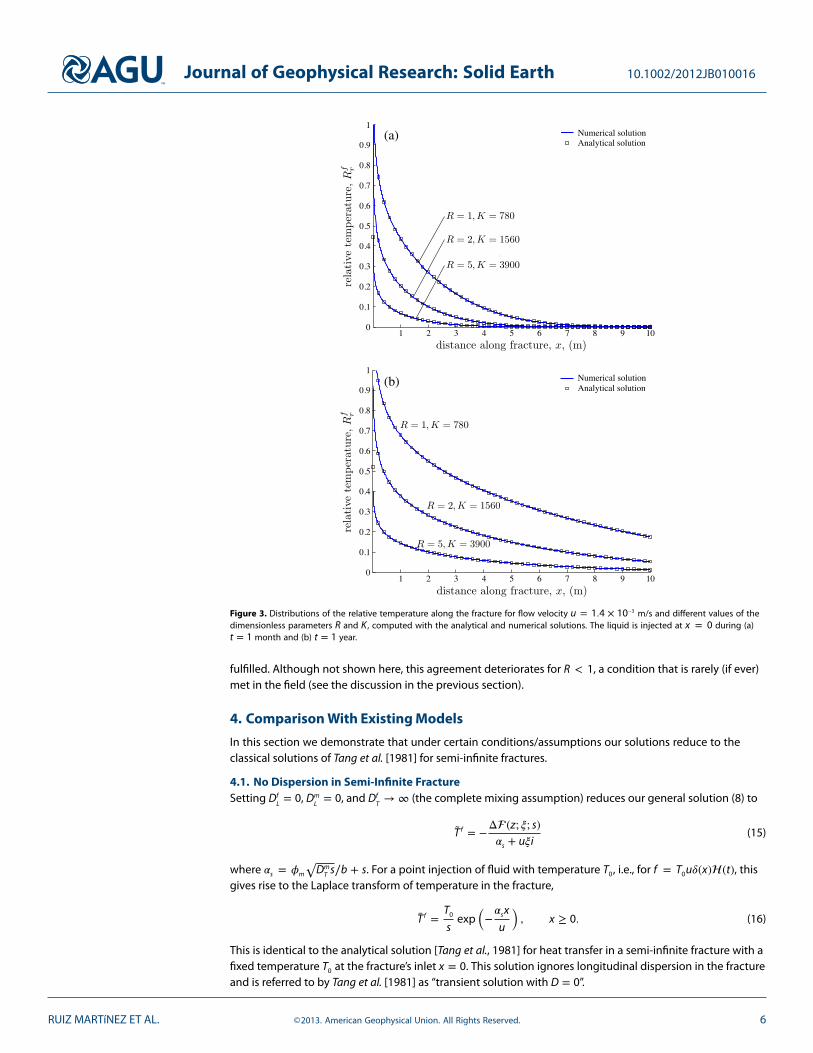
Figure 3. Distributions of the relative temperature along the fracture for flow velocity u = 1.4 × 10−3 m/s and different values of thedimensionless parameters R and K , computed with the analytical and numerical solutions. The liquid is injected at x = 0 during (a)t = 1 month and (b) t = 1 year.

fulfilled. Although not shown here, this agreement deteriorates for R < 1, a condition that is rarely (if ever)met in the field (see the discussion in the previous section).

4. Comparison With Existing Models

In this section we demonstrate that under certain conditions/assumptions our solutions reduce to theclassical solutions of Tang et al. [1981] for semi-infinite fractures.

4.1. No Dispersion in Semi-Infinite FractureSetting Df

L= 0, Dm

L= 0, and Df

T→ ∞ (the complete mixing assumption) reduces our general solution (8) to

T f = −Δ (z; 𝜉; s)𝛼s + u𝜉i

(15)

where 𝛼s = 𝜙m

√Dm

T s∕b + s. For a point injection of fluid with temperature T0, i.e., for f = T0u𝛿(x)(t), thisgives rise to the Laplace transform of temperature in the fracture,

T f =T0

sexp

(−𝛼sx

u

), x ≥ 0. (16)

This is identical to the analytical solution [Tang et al., 1981] for heat transfer in a semi-infinite fracture with afixed temperature T0 at the fracture’s inlet x = 0. This solution ignores longitudinal dispersion in the fractureand is referred to by Tang et al. [1981] as “transient solution with D = 0”.


http://dx.doi.org/10.1002/2012JB010016


4.2. Longitudinal Dispersion in Semi-Infinite FractureSetting Dm

L= 0 and Df

T→ ∞ reduces our general solution (8) to

T f = − Δ (z; 𝜉; s)𝛼s + Df

L𝜉2 + u𝜉i

. (17)

The “general transient solution” of Tang et al. [1981] is recovered from (17) by choosing the source term to be

f =T0

s

√u2 + 4Df

L𝛼s 𝛿(x). (18)

This choice accounts for the “lost” part of the injected flux due to the longitudinal diffusion in the negativehalf (−∞ < x < 0) of the infinite fracture. The resulting Laplace transform of temperature in the fracture is

T f =T0

sexp

[−

(√u2

4+ Df

L𝛼s −u2

)x

DfL

], x ≥ 0. (19)

5. Results and Discussion

The subsequent discussion serves to demonstrate the importance of accounting for two-dimensionalheat conduction in rock matrix. In this discussion, we refer to (13) and (16) as “2-D solution” and“1-D solution,” respectively.

The results below correspond to continuous point injection (x = 0) of a fluid whose temperature T0 is eitherwarmer (T0 > 0) or colder (T0 < 0) than the host fluid (the initial temperature Ti = 0). Unless specifiedotherwise, a shale matrix has the following characteristics: Dm

L= Dm

T= 9.16×10−7 m2/s, 𝜙 = 0.1, 𝜌s = 2757

kg/m3, and cs = 1180 J/kg K. Taking the fluid to be water (𝜌f = 1070 kg/m3 and cf = 4050 J/kg K) yields𝜙m = [𝜙 + (1 − 𝜙)𝜌scs∕(𝜌f cf )] = 0.78.

The results are reported in terms of the relative fracture temperature

T fr(x, t) = T f (x, t)∕T0, (20)

which ranges from 0 (temperature is at its initial value Ti) to 1 (temperature at the local heat source).

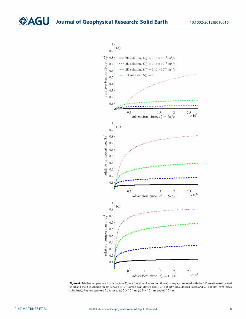
5.1. Effects of Heat Conduction in MatrixFigure 4 depicts the temporal evolution of relative temperature T f

rat the distance x = 0.5 m from the heat

source. Flow velocity in the fracture is set to u = 1.4 × 10−4 m/s, and fracture aperture to 2b = 2 × 10−4 m(Figure 4a), 5 × 10−4 m (Figure 4b), and 10−3 m (Figure 4c). This choice of fracture apertures yields the valuesof the dimensionless ratio R = 50 (Figure 4a), R = 20 (Figure 4b), and R = 10 (Figure 4c).

In the diffusion-dominated regime (Figure 4a), the 1-D solution (no longitudinal heat conduction in thematrix) underestimates the relative temperature at short times and significantly overestimates it at latertimes. The longitudinal heat conduction in the matrix (the 2-D solution) causes the fracture temperature torise at earlier times and shows that the local heat source impacts on the fracture temperature (T f

r> 0) at

much earlier times; after this initial time interval, the 1-D solution predicts a much larger rate of increase ofthe fracture temperature than the 2-D solutions do. This is because heat is transferred from the fracture intothe matrix in the vicinity of the localized injection, diffuses longitudinally in the matrix, and then returnsto the fracture at locations far from the injection. Our 2-D solution captures this heat transfer mechanism inthe diffusion-dominated regime, while the classical 1-D solution does not. Figures 4b and 4c show that thismechanism does not occur in advection-dominated regimes.

In all heat transfer regimes (Figures 4a–4c), both temperature in the fracture and the time-to-equilibriumincrease as the matrix diffusion coefficient Dm

Ldecreases. The smaller the value of R (i.e., the larger the

fracture-matrix Péclet number), the more pronounced this effect becomes. Ignoring longitudinal diffusionin the matrix (the 1-D solution) significantly underestimates the fracture-matrix transfer and significantlyoverestimates both temperature in the fracture and the time-to-equilibrium.

Overestimation of the time-to-equilibrium has important practical implications, since determination of thetime it takes a fracture-matrix system to reach thermal equilibrium (steady state) is essential for estimationof the matrix penetration depth. The latter determines the adequacy of conceptual representations of


http://dx.doi.org/10.1002/2012JB010016


(a)

(b)

(c)

Figure 4. Relative temperature in the fracture T fr, as a function of advection time t∗

a= tu∕x, computed with the 1-D solution (red dotted

lines) and the 2-D solution for DmL= 9.16×10−9 (green dash-dotted lines), 9.16×10−8 (blue dashed lines), and 9.16×10−7 m2/s (black

solid lines). Fracture aperture 2b is set to (a) 2 × 10−4 m, (b) 5 × 10−4 m, and (c) 10−3 m.


http://dx.doi.org/10.1002/2012JB010016


(a)

(b)

(c)

Figure 5. Isolines of the geothermal performance Pf in the space of advection (t∗a) and diffusion (t∗

d) times, for (a) R = 1, (b) R = 2, and

(c) R = 5.


http://dx.doi.org/10.1002/2012JB010016


(a)

(b)

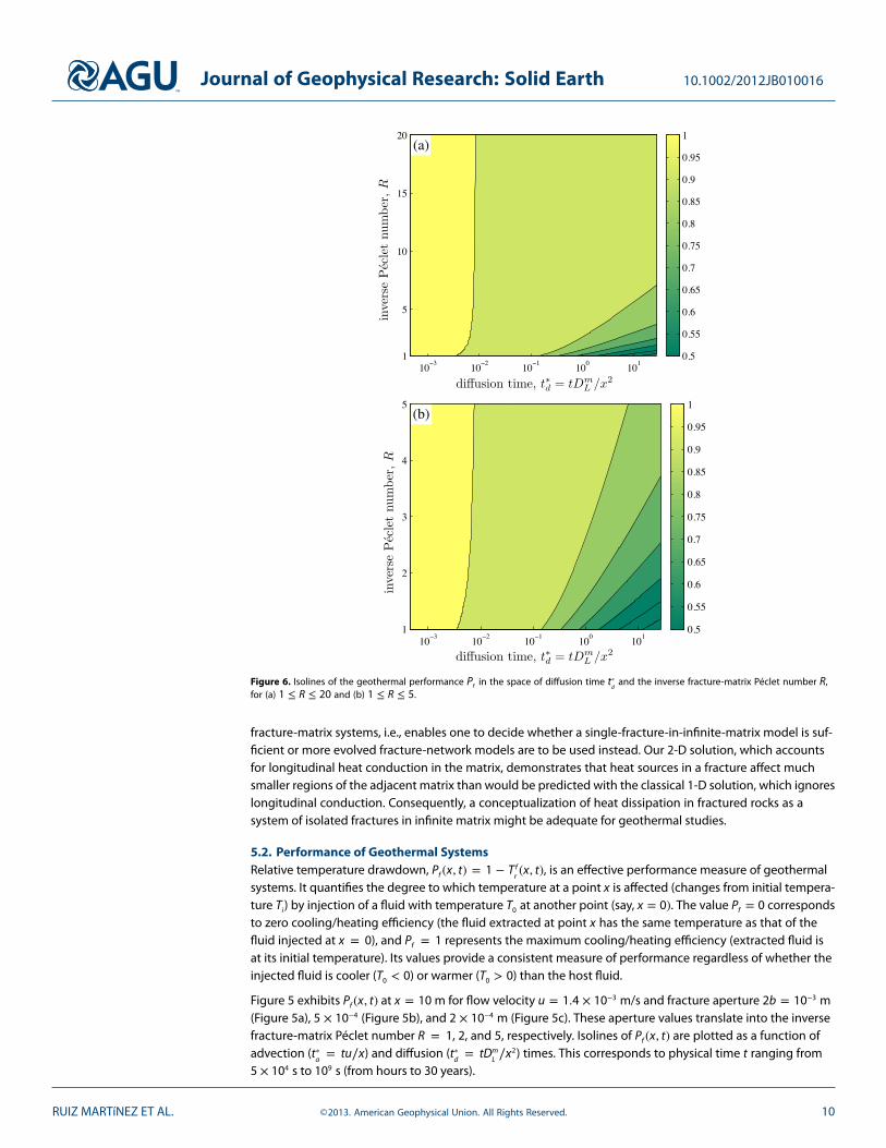
Figure 6. Isolines of the geothermal performance Pf in the space of diffusion time t∗d

and the inverse fracture-matrix Péclet number R,for (a) 1 ≤ R ≤ 20 and (b) 1 ≤ R ≤ 5.

fracture-matrix systems, i.e., enables one to decide whether a single-fracture-in-infinite-matrix model is suf-ficient or more evolved fracture-network models are to be used instead. Our 2-D solution, which accountsfor longitudinal heat conduction in the matrix, demonstrates that heat sources in a fracture affect muchsmaller regions of the adjacent matrix than would be predicted with the classical 1-D solution, which ignoreslongitudinal conduction. Consequently, a conceptualization of heat dissipation in fractured rocks as asystem of isolated fractures in infinite matrix might be adequate for geothermal studies.

5.2. Performance of Geothermal SystemsRelative temperature drawdown, Pf (x, t) = 1 − T f

r(x, t), is an effective performance measure of geothermal

systems. It quantifies the degree to which temperature at a point x is affected (changes from initial tempera-ture Ti) by injection of a fluid with temperature T0 at another point (say, x = 0). The value Pf = 0 correspondsto zero cooling/heating efficiency (the fluid extracted at point x has the same temperature as that of thefluid injected at x = 0), and Pf = 1 represents the maximum cooling/heating efficiency (extracted fluid isat its initial temperature). Its values provide a consistent measure of performance regardless of whether theinjected fluid is cooler (T0 < 0) or warmer (T0 > 0) than the host fluid.

Figure 5 exhibits Pf (x, t) at x = 10 m for flow velocity u = 1.4 × 10−3 m/s and fracture aperture 2b = 10−3 m(Figure 5a), 5 × 10−4 (Figure 5b), and 2 × 10−4 m (Figure 5c). These aperture values translate into the inversefracture-matrix Péclet number R = 1, 2, and 5, respectively. Isolines of Pf (x, t) are plotted as a function ofadvection (t∗

a= tu∕x) and diffusion (t∗

d= tDm

L∕x2) times. This corresponds to physical time t ranging from

5 × 104 s to 109 s (from hours to 30 years).


http://dx.doi.org/10.1002/2012JB010016


Geothermal performance increases with R: it is lowest in the advection-dominated regime (Figure 5a) andhighest in the diffusion-dominated regime (Figure 5c). In a given regime (as characterized by the value of R),the performance varies only slightly with t∗

a, i.e., it is relatively insensitive to convective properties of frac-

tured rocks. This is to be expected from Figure 4, which shows that temperature in the fracture stabilizesquickly as the advection time t∗

aincreases, so that subsequent increases in t∗

ahave a limited impact on

system performance.

When R = (1), the geothermal performance Pf depends strongly on the diffusion time t∗d, with high perfor-

mance occurring at small values of t∗d. Therefore, the cooling/heating efficiency increases with the reservoir

size (the distance x between fluid’s injection and extraction) and decreases with exploitation time t. As Rincreases (from R = 1 in Figure 5a to R = 5 in Figure 5c), the dependence of the geothermal performance Pf

on t∗d

diminishes, leading to stable and efficient configurations in the diffusion-dominated regime. For largevalues of t∗

d(the top of Figures 5a–5c), the geothermal performance is slightly higher at small values of t∗

a.

This implies that for rocks with large thermal diffusivity DmL

(large values of t∗d), the largest changes in fluid

temperature in the fracture occur at early times ta and the geothermal performance can be improved bydecreasing flow velocity u.

Figure 6 illustrates these points further. Extracted fluid remains at its initial temperature regardless of thetemperature of injected fluid for t∗

d< 10−2. The latter inequality holds for small values of Dm

L, short exploita-

tion times t, and/or large distances (x) between the injection and extraction points. This nearly perfectgeothermal performance (Pf > 0.9) is observed when R > 7. In other words, the diffusion-dominatedregime is best suited for geothermal exploitation, since it limits the thermal impact of injected fluids on thehost fluid in a fracture by maximizing heat dissipation into the matrix. In the advection-dominated regimewith R < 5 (Figure 6b), the geothermal performance depends strongly on t∗

d, with small values of t∗

d(short

exploitation times t or/and large injection-to-extraction distances x) improving Pf .

6. Conclusions

We developed analytical models for heat transfer in a single fracture surrounded by an infinite matrix. Thesemodels account for advection and hydrodynamic dispersion in the fracture, longitudinal and transverseconduction in the matrix, and a two-way coupling between heat transfer in the fracture and matrix. Theyalso handle any heat source configuration, such as distributed or localized heat sources of arbitrary duration.

In their most general form, these solutions are given by their Fourier and Laplace transforms and requirenumerical inversion. Under conditions that are typical of geothermal reservoirs, these solutions are invertedanalytically, giving rise to an explicit closed-form model of heat transfer in fractured rocks. By accountingfor two-dimensional heat conduction in rock matrix, this model represents a significant advance over theexisting analytical solutions that restrict matrix conduction to the direction perpendicular to the fracture.Our analysis leads to the following major conclusions.

1. Longitudinal thermal diffusivity in the matrix is a critical parameter that determines the impact of localheat sources on fluid temperature in the fracture.

2. By neglecting longitudinal conduction in the matrix, the classical models significantly overestimate bothfracture temperature and time-to-equilibrium.

3. The inverse fracture-matrix Péclet number R and diffusion timescale t∗d

are two parameters that determinethe efficiency of geothermal systems.

4. The diffusion-dominated regime (R > 7) is ideal for geothermal exploitation, since it limits the thermalimpact of injected fluids on the host fluid in a fracture by maximizing heat dissipation into the matrix.

5. In the advection-dominated regime (R < 5), the geothermal performance depends strongly on t∗d. It is

highest at small values of t∗d

(short exploitation times and/or large injection-to-extraction distances).

Our analytical models provide an easy-to-use tool for parametric sensitivity analysis, benchmark studies,and validation of numerical simulations. They can be used for geothermal site evaluation and parameteridentification. They will improve field-scale studies of geothermal reservoirs, which rely on discrete frac-ture network approaches and consider only one-dimensional heat conduction in the rock. Our solutionsobviate the need for this strong and limiting assumption, while retaining the analytic simplicity of theoriginal approaches.


http://dx.doi.org/10.1002/2012JB010016


In the follow-up studies, we will generalize these analytical models by incorporating the followingphenomena.

1. Fracture wall roughness. The numerical simulations of Neuville et al. [2010] demonstrated the effects offracture wall roughness on heat transfer in fractured rocks. Treating fracture walls as random fields, andcombining our solutions with stochastic domain mappings [Xiu and Tartakovsky, 2006; Tartakovsky andXiu, 2006; Park et al., 2012] and stochastic homogenization [Tartakovsky et al., 2003], will enable us toinvestigate these effects in a computationally efficient semi-analytical manner. The latter step will rely onthe Green’s functions derived in this study.

2. Heat transfer in fracture networks. Multiscale modeling approaches to flow and transport in fracturedrocks [e.g., Dershowitz and Miller, 1995; Cvetkovic et al., 2004; Roubinet et al., 2010, 2013] combine a dis-crete fracture network (DFN) representation at the field scale with analytical solutions at the fracture scale.We will embed our analytical solutions into particle-tracking DFN models to represent rock conductioneffects at the field scale with optimized computational cost and representation accuracy.

Appendix A: Green’s Functions

A1. Green’s Function for Fracture BVP

We represent the two-dimensional Green’s function Gf as the product of two one-dimensional Green’sfunctions, Gf = Gf

x(x; x′; t − t′)Gf

z(z; z′; t − t′) [Carslaw and Jaeger, 1959]

Gfx= 1

2√𝜋Df

L(t − t′)exp

[−[x′ − x + u(t − t′)]2

4DfL(t − t′)

](A1)

and

Gfz= 1

b+ 2

b

∞∑n=1

e−𝛼2n Df

T(t−t′) cos(𝛼nz) cos(𝛼nz′) (A2)

where 𝛼n = n𝜋∕b. The Fourier Laplace (FL) transform of Gf has the form

Gf =Gf𝜉(s)√

2𝜋b+√

2𝜋

∞∑n=1

cos(𝛼nz) cos(𝛼nz′)b

Gf𝜉(s + 𝛼2

nDf

T) (A3)

where

Gf𝜉(s) = 1

s + 𝜉2DfL + u𝜉i

. (A4)

A2. Green’s Function for Matrix BVP

The Green’s function Gm is computed as the product of one-dimensional Green’s functions, Gm = Gmx(x; x′;

t − t′)Gmz(z; z′; t − t′),

Gmx= 1

2√𝜋Dm

L (t − t′)exp

[−(x′ − x)2

4DmL (t − t′)

](A5)

and

Gmz= e−(z′−z)2∕𝜔 + e−(z′+z−2b)2∕𝜔

2√𝜋Dm

T (t − t′)(A6)

where 𝜔 = 4DmT(t − t′). The FL transform of Gm is

Gm = e−𝜓|z−z′|∕√Dm

T + e−𝜓|z+z′−2b|∕√Dm

T

2√

2𝜋DmT 𝜓

(A7)

where 𝜓 =√

DmL 𝜉

2 + s.


http://dx.doi.org/10.1002/2012JB010016


Appendix B: Integral Solutions of BVPs

Solutions of the fracture and matrix BVPs, expressed in terms of the Green’s functions, are

T f (x, z, t) =

t

∫0

∞

∫−∞

r(x′, t′)Gf (.; x′, b; .)dx′dt′

+

t

∫0

b

∫0

∞

∫−∞

f (x′, z′, t′)Gf (.; .; .)dx′dz′dt′

(B1)

and

T m(x, z, t) = − 1𝜙m

t

∫0

∞

∫−∞

r(x′, t′)Gm(.; x′, b; .)dx′dt′. (B2)

Their FL transforms are

T f =√

2𝜋⎛⎜⎜⎝rGf |z′=b +

b

∫0

f Gf dz′⎞⎟⎟⎠ (B3)

T m = −

√2𝜋 rGm|z′=b

𝜙m

, (B4)

where Gf and Gm are given by (A3) and (A7), respectively.

The FL transform of the fracture-matrix heat transfer, r(𝜉, s), is obtained from the continuity condition at theinterface, T f (𝜉, z = b, s) = T m(𝜉, z = b, s).

Appendix C: Fourier-Laplace Inversions

Since T f (𝜉, s) = T∗(−𝜉, s) (where T∗ denotes the conjugate of T f ), the inverse Fourier transform of T f is

T f = 1√2𝜋

∞

∫0

[T∗(𝜉, s)e−ix𝜉 + T f (𝜉, s)eix𝜉

]d𝜉 (C1)

and its inverse Laplace transform is

T f = 1√2𝜋

∞

∫0

[L−1[T∗]e−ix𝜉 + L−1[T f ]eix𝜉

]d𝜉 (C2)

where L−1[ ] represents the inverse Laplace operator.

C1. Inverse Laplace Transform of Tf

We decompose the FL transform T f in (11) into simple fractions

T f = A4∑

i=1

Xi

𝜓 + bi

, A =T0u√

2𝜋(C3)

where b1 = B∕2 +√

G − Di, b2 = B∕2 −√

G − Di, b3 = −b4 =√

C, X1 = 1∕[(b1 − b2)(C − b21)], X2 =

−1∕[(b1−b2)(C−b22)], X3 = −1∕2

√C[(C+b1b2)−(b1+b2)

√C], X4 = 1∕2

√C[(C+b1b2)+(b1+b2)

√C], and

B =𝜙m

√Dm

T

b, C = Dm

L𝜉2, D = u𝜉, G = B2

4+ C. (C4)

Since only 𝜓 =√

C + s depends on the Laplace variable s, and noticing that∑4

i=1Xi = 0, the inverse Laplace

of T f is

T f = −Ae−Ct

4∑i=1

Xibieb2

iterfc(bi

√t) (C5)


http://dx.doi.org/10.1002/2012JB010016


which can be recast in terms of the function w(z) = e−z2 erfc(−iz) of a complex variable z [Faddeeva andTerent’tev, 1961] as

T f =AB

√C

B2C + D2

[1 − erfc(

√Ct)

]− ADi

B2C + D2

[1 − e−Ctw(ib1

√t)]

+ AX2b2e−Ct[

w(ib1

√t) − w(ib2

√t)].

(C6)

C2. Inverse Fourier Transform of Tf

Recalling that b1 and b2 in (C6) are given by

b1 =B2+

√√G2 + D2 + G

2− i

√√G2 + D2 − G

2(C7)

b2 =B2−

√√G2 + D2 + G

2+ i

√√G2 + D2 − G

2, (C8)

expanding the square roots into Taylor series, and requiring G ≫ D leads to

b1 ≈B2+√

G + D2

4G− iD

2√

G, b2 ≈

B2−√

G + D2

4G+ iD

2√

G. (C9)

Requiring B2∕4 ≫ C, and expanding the square roots into Taylor series, yields

b1 ≈ B − iDB, b2 ≈ −C

B− D2

B3+ i

DB. (C10)

Similarly, X2b2 in (C6) is approximated by

X2b2 ≈1B2

− iDB2C + D2

. (C11)

Finally, for small values of 𝜉, we approximate b1 and b2 in the arguments of w(⋅) with b1 ≈ B and b2 ≈ iD∕B,so that

w(ib1

√t) ≈ eB2 terfc(B

√t)

w(ib2

√t) ≈ e−D2 t∕B2

erfc(iD√

t∕B).(C12)

For t > 104∕B2, expanding erfc(iD√

t∕B) into a Taylor series yields

w(ib1

√t) ≈ 0

w(ib2

√t) ≈ e−𝜀2

[1 −

(2√𝜋𝜀 + 2

3√𝜋𝜀3 + 1

5√𝜋𝜀5

)i

],

(C13)

where 𝜀 = D√

t∕B. With these approximations, (C6) is replaced with

T f ≈A√

CB2𝜅

erf(√

Ct) − ADiB2𝜅

− A(𝜅 − Di)B2𝜅

[1 −

(2𝜀√𝜋+ 2𝜀3

3√𝜋+ 𝜀5

5√𝜋

)i

]e−𝜅t (C14)

where 𝜅 = C + D2∕B2. Using (C2) to compute the inverse Fourier transform leads to (13).

C3. Limits of Applicability of Analytical Model (13)

The Fourier transform of temperature in the fracture (C14) and its exact analytical inversion (13) are derivedunder the following three conditions:

1. B2∕4 + C ≫ D2. B2∕4 ≫ C3. t > 104∕B2.

In what follows, we demonstrate the general applicability of these conditions.


http://dx.doi.org/10.1002/2012JB010016


Condition 1: Solving the first condition B2∕4 + C ≫ D as an equation results in

𝜉2 = u2

2DmL

2−𝜙2

mDm

T

4b2DmL

± u2Dm

L2

√u2 −

𝜙2m

DmL Dm

T

b2. (C15)

Thus, 𝜉 is real if

𝜙m

√Dm

L DmT

ub> 1. (C16)

Condition 2: Recalling (C4), this condition implies 𝜉2 ≪ 𝜙2m

DmT∕(4Dm

Lb2). When 𝜉 > 1, this is equivalent to

𝜉 < 𝜙m

√Dm

T ∕DmL ∕(2b), which gives

𝜙m

2b

√DT

m

DLm

> 1. (C17)

Condition 3: For B2t = 104, eB2 terfc(√

B2t) ≈ 0.0056 and we treat it as 0. This yields a third constraint,

t >104b2

𝜙2m

DmT

. (C18)

ReferencesAl-Hadhrami, H. S., and M. J. Blunt (2001), Thermally induced wettability alteration to improve oil recovery in fractured reservoirs, SPE

Reserv. Eval. Eng., 4(3), 179–186.Baston, D. P., and B. H. Kueper (2009), Thermal conductive heating in fractured bedrock: Screening calculations to assess the effect of

groundwater influx, Adv. Water Resour., 32, 231–238.Bataillé, A., P. Genthon, M. Rabinowicz, and B. Fritz (2006), Modeling the coupling between free and forced convection in a vertical

permeable slot: Implications for the heat production of an enhanced geothermal system, Geothermics, 35, 654–682.Bodvarsson, G. S., and C. F. Tsang (1982), Injection and thermal breakthrough in fractured geothermal reservoirs, J. Geophys. Res., 87(NB2),

1031–1048.Carslaw, H. S., and J. C. Jaeger (1959), Conduction of Heat in Solids, Oxford Univ. Press, New York.Chen, X., and P. M. Shearer (2011), Comprehensive analysis of earthquake source spectra and swarms in the Salton Trough, California, J.

Geophys. Res., 116, B09309, doi:10.1029/2011JB008263.Cheng, A. H.-D., A. Ghassemi, and E. Detournay (2001), Integral equation solution of heat extraction from a fracture in hot dry rocks, Int.

J. Numer. Anal. Methods Geomech., 25(13), 1327–1338.Cvetkovic, V., S. Painter, N. Outters, and J. O. Selroos (2004), Stochastic simulation of radionuclide migration in discretely fractured rock

near the Aspo Hard Rock Laboratory, Water Resour. Res., 40, W02404, doi:10.1029/2003WR002655.de Hoog, F. R., J. H. Knight, and A. N. Stokes (1982), An improved method for numerical inversion of Laplace transforms, SIAM J. Sci.

Comput., 3(3), 357–366.Dershowitz, W., and I. Miller (1995), Dual-porosity fracture flow and transport, Geophys. Res. Lett., 22(11), 1441–1444.Faddeeva, V. N., and N. M. Terent’tev (1961), Tables of Values of the Function w(z) for Complex Argument, Pergamon Press, New York.Gelet, R., B. Loret, and N. Khalili (2012), A thermo-hydro-mechanical coupled model in local thermal non-equilibrium for fractured HDR

reservoir with double porosity, J. Geophys. Res., 117, B07205, doi:10.1029/2012JB009161.Gringarten, A. C., P. A. Witherspoon, and Y. Ohnishi (1975), Theory of heat extraction from fractured hot dry rock, J. Geophys. Res., 80(8),

1120–1124.Gunasekera, R. C., G. R. Foulger, and B. R. Julian (2003), Reservoir depletion at The Geysers geothermal area, California, shown by

four-dimensional seismic tomography, J. Geophys. Res., 108(B3), 2134, doi:10.1029/2001JB000638.Kolditz, O. (1995), Modeling flow and heat-transfer in fractured rocks: Dimensional effect of matrix heat diffusion, Geothermics, 24(3),

421–437.Lin, W. (2002), Permanent strain of thermal expansion and thermally induced microcracking in Inada granite, J. Geophys. Res., 107(B10),

2215, doi:10.1029/2001JB000648.Meyer, J. (2004), Development of a heat transport analytical model for a single fracture in a porous matrix, Report for Earth 661,

University of Waterloo.Molson, J., P. Pehme, J. Cherry, and B. Parker (2007), Numerical analysis of heat transport within fractured sedimentary rock: Implications

for temperature probes, paper presented at NGWA/U.S.EPA Fractured Rock Conference: State of the Science and Measuring Success inRemediation, vol. 5017, Portland, Maine.

Neuville, A., R. Toussaint, and J. Schmittbuhl (2010), Hydrothermal coupling in a self-affine rough fracture, 82, 036,317, doi:10.1103/PhysRevE.82.036317.

Park, S.-W., M. Intaglietta, and D. M. Tartakovsky (2012), Impact of endothelium roughness on blood flow, J. Theor. Biol., 300, 152–160,doi:10.1016/j.jtbi.2012.01.017.

Pehme, P. E., J. P. Greenhouse, and B. L. Parker (2007), The active line source temperature logging technique and its application infractured rock hydrogeology, J. Environ. Eng. Geophys., 12, 307–322.

Pehme, P. E., B. L. Parker, J. A. Cherry, and J. P. Greenhouse (2010), Improved resolution of ambient flow through fractured rock withtemperature logs, Ground Water, 48, 191–205.

Roubinet, D., H.-H. Liu, and J.-R. de Dreuzy (2010), A new particle-tracking approach to simulating transport in heterogeneous fracturedporous media, Water Resour. Res., 46, W11507, doi:10.1029/2010WR009371.

AcknowledgmentsThis work was supported in part bythe National Science Foundationaward EAR-1246315 and by the Com-putational Mathematics Programof the Air Force Office of ScientificResearch.


http://dx.doi.org/10.1002/2012JB010016

http://dx.doi.org/10.1029/2011JB008263

http://dx.doi.org/10.1029/2003WR002655

http://dx.doi.org/10.1029/2012JB009161

http://dx.doi.org/10.1029/2001JB000638

http://dx.doi.org/10.1029/2001JB000648

http://dx.doi.org/10.1103/\penalty -\@M PhysRevE.82.036317

http://dx.doi.org/10.1016/j.jtbi.2012.01.017

http://dx.doi.org/10.1029/2010WR009371


Roubinet, D., J.-R. de Dreuzy, and D. M. Tartakovsky (2012), Semi-analytical solutions for solute transport and exchange in fracturedporous media, Water Resour. Res., 48, W01542, doi:10.1029/2011WR011168.

Roubinet, D., J.-R. de Dreuzy, and D. M. Tartakovsky (2013), Particle-tracking simulations of anomalous transport in hierarchicallyfractured rocks, Comput. Geosci., 50, 52–58.

Sudicky, E. A., and E. O. Frind (1982), Contaminant transport in fractured porous-media: Analytical solutions for a system of parallelfractures, Water Resour. Res., 18(6), 1634–1642.

Tang, D. H., E. O. Frind, and E. A. Sudicky (1981), Contaminant transport in fractured porous-media: Analytical solution for a singlefracture, Water Resour. Res., 17(3), 555–564.

Tartakovsky, D. M., and D. Xiu (2006), Stochastic analysis of transport in tubes with rough walls, J. Comput. Phys., 217, 248–259.Tartakovsky, D. M., A. Guadagnini, and M. Riva (2003), Stochastic averaging of nonlinear flows in heterogeneous porous media, J. Fluid

Mech., 492, 47–62, doi:10.1017/S002211200300538X.Wang, H. F., B. P. Bonner, S. R. Carlson, B. J. Kowallis, and H. C. Heard (1989), Thermal-stress cracking in granite, J. Geophys. Res., 94(B2),

1745–1758.Wang, J. S. Y., C. F. Tsang, N. G. W. Cook, and P. A. Witherspoon (1981), A study of regional temperature and thermohydrologic effects of

an underground repository for nuclear wastes in hard rock, J. Geophys. Res., 86(NB5), 3759–3707.Willis-Richards, J., K. Watanabe, and H. Takahashi (1996), Progress toward a stochastic rock mechanics model of engineered geothermal

systems, J. Geophys. Res., 101(B8), 17,481–17,496.Xiang, Y., and Y. Zhang (2012), Two-dimensional integral equation solution of advective-conductive heat transfer in sparsely fractured

water-saturated rocks with heat source, Int. J. Geomech., 12, 168–175.Xiu, D., and D. M. Tartakovsky (2006), Numerical methods for differential equations in random domains, SIAM J. Sci. Comput., 28(3),

1167–1185.Xu, T. F., and K. Pruess (2001), On fluid flow and mineral alteration in fractured caprock of magmatic hydrothermal systems, J. Geophys.

Res., 106(B2), 2121–2138.Yang, S.-Y., and H.-D. Yeh (2009), Modeling heat extraction from hot dry rock in a multi-well system, Appl. Therm. Eng., 29, 1676–1681.Zhou, Q., H.-H. Liu, F. J. Molz, Y. Zhang, and G. S. Bodvarsson (2007), Field-scale effective matrix diffusion coefficient for fractured rock:

Results from literature survey, J. Contam. Hydrol., 93, 161–187.


http://dx.doi.org/10.1002/2012JB010016

http://dx.doi.org/10.1029/2011WR011168

http://dx.doi.org/10.1017/S002211200300538X

analytical models of heat conduction in fractured...

Documents