analytical foundations of physical security system...
TRANSCRIPT

ANALYTICAL FOUNDATIONS OF
PHYSICAL SECURITY SYSTEM ASSESSMENT
A Dissertation
by
GREGORY HOWARD GRAVES
Submitted to the Office of Graduate Studies ofTexas A&M University
in partial fulfillment of the requirements for the degree of
DOCTOR OF PHILOSOPHY
August 2006
Major Subject: Industrial Engineering

ANALYTICAL FOUNDATIONS OF
PHYSICAL SECURITY SYSTEM ASSESSMENT
A Dissertation
by
GREGORY HOWARD GRAVES
Submitted to the Office of Graduate Studies ofTexas A&M University
in partial fulfillment of the requirements for the degree of
DOCTOR OF PHILOSOPHY
Approved by:
Chair of Committee, Martin A. WortmanCommittee Members, J. Eric Bickel
Daren B.H. ClineDonald R. Smith
Head of Department, Brett A. Peters
August 2006
Major Subject: Industrial Engineering

iii
ABSTRACT
Analytical Foundations of
Physical Security System Assessment. (August 2006)
Gregory Howard Graves, B.S., United States Military Academy;
M.S., Texas A&M University
Chair of Advisory Committee: Dr. Martin A. Wortman
Physical security systems are intended to prevent or mitigate potentially catas-
trophic loss of property or life. Decisions regarding the selection of one system or
configuration of resources over another may be viewed as design decisions within a
risk theoretic setting. The problem of revealing a clear preference among design alter-
natives, using only a partial or inexact delineation of event probabilities, is examined.
In this dissertation, an analytical framework for the assessment of the risk as-
sociated with a physical security system is presented. Linear programming is used
to determine bounds on the expected utility of an alternative, and conditions for
the separation of preferences among alternatives are shown. If distinguishable pref-
erences do not exist, techniques to determine what information may help to separate
preferences are presented. The linear programming approach leads to identification
of vulnerabilities in a security system through an examination of the solution to the
dual problem.
Security of a hypothetical military forward operating base is considered as an
illustrative example. For two alternative security schemes, the uncertainty inherent in
the scenario is represented using probability assessments consisting of bounds on event
probabilities and exact probability assignments. Application of the framework reveals
no separation of preferences between the alternatives. Examination of the primal and

iv
dual solutions to the linear programming problems, however, reveals insights into
information which, if obtained, could lead to a separation of preferences as well as
information on vulnerabilities in one of the alternative security postures.

v
To Wya, one of my foremost sources of certainty.

vi
ACKNOWLEDGMENTS
I offer my sincere thanks to Dr. Martin A. Wortman, Dr. Daren B. H. Cline,
Dr. Donald R. Smith, and Dr. J. Eric Bickel for serving on my advisory committee
and for insisting on excellence.
I would like to express particular appreciation to Dr. Wortman, my committee
chair. His patience, confidence, insights, and expertise were foundational throughout
the uncertainty faced in the completion of this effort.
I owe much gratitude to my wife, Wya, for carrying more than her fair share,
and to my children, Abigail, Sarah, AnnaBeth, and Hope, for their unwavering love,
patience, and understanding throughout the process.
I thank my parents for infusing me with the motivation to learn, to excel, and
to balance the important things in life.
Finally, I offer my appreciation to the U.S. Army, the U.S. Military Academy, and
the Department of Mathematical Sciences at West Point for this amazing opportunity
that has stretched me and given me additional appreciation for what we do.

vii
TABLE OF CONTENTS
CHAPTER Page
I INTRODUCTION . . . . . . . . . . . . . . . . . . . . . . . . . . 1
A. Physical Security Principles . . . . . . . . . . . . . . . . . 3
1. Asset Identification . . . . . . . . . . . . . . . . . . . 3
2. Threats . . . . . . . . . . . . . . . . . . . . . . . . . . 4
3. Threat Evaluation . . . . . . . . . . . . . . . . . . . . 4
4. Risk Mitigation . . . . . . . . . . . . . . . . . . . . . 5
5. Constraints . . . . . . . . . . . . . . . . . . . . . . . . 5
6. Evaluation of Alternatives . . . . . . . . . . . . . . . . 6
7. Decide, Implement, and Monitor . . . . . . . . . . . . 6
B. Objectives and Approach . . . . . . . . . . . . . . . . . . . 6
1. Research Objectives . . . . . . . . . . . . . . . . . . . 7
2. Approach . . . . . . . . . . . . . . . . . . . . . . . . . 8
C. Dissertation Organization . . . . . . . . . . . . . . . . . . 9
II LITERATURE REVIEW . . . . . . . . . . . . . . . . . . . . . . 10
A. Modeling of Physical Security, Antiterrorism, and Force
Protection Systems . . . . . . . . . . . . . . . . . . . . . . 10
B. Decisions in the Absence of a Unique Probability Measure 13
C. Security Decision Training: Fields and Needs . . . . . . . . 16
III RISK ASSESSMENT OF SECURITY SYSTEMS . . . . . . . . 20
A. The Expected Utility Theorem . . . . . . . . . . . . . . . . 20
B. Separation of Risk Preferences Using Sets of Probability Laws 23
C. Physical Security Decisions . . . . . . . . . . . . . . . . . . 25
IV ASSESSMENT OF PHYSICAL SECURITY SYSTEMS . . . . . 29
A. Loss Uncertainty . . . . . . . . . . . . . . . . . . . . . . . 30
B. Expected Utility of Alternatives . . . . . . . . . . . . . . . 32
C. Alternatives Having the Most Preferred Risk . . . . . . . . 35
D. Linear Programming Formulation . . . . . . . . . . . . . . 37
E. Dual Problem Solutions . . . . . . . . . . . . . . . . . . . 40
1. Bounds on Event Probabilities . . . . . . . . . . . . . 41
2. Bounds on Conditional Probabilities . . . . . . . . . . 43

viii
CHAPTER Page
F. Independence . . . . . . . . . . . . . . . . . . . . . . . . . 45
V AN APPLICATION IN A MILITARY SCENARIO . . . . . . . 48
A. Background and Scenario Setting . . . . . . . . . . . . . . 48
B. Intelligence Assessment . . . . . . . . . . . . . . . . . . . . 51
C. Description of Alternatives . . . . . . . . . . . . . . . . . . 53
D. Determining Sets of Distributions on Loss . . . . . . . . . 53
E. Analysis of Results . . . . . . . . . . . . . . . . . . . . . . 57
1. Insight from the Dual Solutions . . . . . . . . . . . . . 57
a. Dual Values as Shadow Prices . . . . . . . . . . . 57
b. Shadow Pricing for Conditional Probabilities . . . 58
2. Consistency and the Primal Solutions . . . . . . . . . 63
VI CONCLUSION . . . . . . . . . . . . . . . . . . . . . . . . . . . 66
A. Future Research Areas . . . . . . . . . . . . . . . . . . . . 67
1. Problem Description . . . . . . . . . . . . . . . . . . . 68
2. Formulation of Bilinear Programs . . . . . . . . . . . 69
B. Concluding Remarks . . . . . . . . . . . . . . . . . . . . . 71
1. Motivation and Flow of Research . . . . . . . . . . . . 71
2. Further Areas for Application . . . . . . . . . . . . . . 73
REFERENCES . . . . . . . . . . . . . . . . . . . . . . . . . . . . . . . . . . . 75
APPENDIX A . . . . . . . . . . . . . . . . . . . . . . . . . . . . . . . . . . . 84
APPENDIX B . . . . . . . . . . . . . . . . . . . . . . . . . . . . . . . . . . . 87
APPENDIX C . . . . . . . . . . . . . . . . . . . . . . . . . . . . . . . . . . . 91
APPENDIX D . . . . . . . . . . . . . . . . . . . . . . . . . . . . . . . . . . . 92
VITA . . . . . . . . . . . . . . . . . . . . . . . . . . . . . . . . . . . . . . . . 100

ix
LIST OF TABLES
TABLE Page
I Scenario Attack Types . . . . . . . . . . . . . . . . . . . . . . . . . . 52
II Sector Values (in $ thousands) . . . . . . . . . . . . . . . . . . . . . 54
III Possible Values of Li . . . . . . . . . . . . . . . . . . . . . . . . . . . 54
IV Conditional Probability Constraint Shadow Prices . . . . . . . . . . . 62
V Probability of Destruction of Sector 3 . . . . . . . . . . . . . . . . . 64

x
LIST OF FIGURES
FIGURE Page
1 Physical Security Design Process . . . . . . . . . . . . . . . . . . . . 7
2 Perimeter of Forward Operating Base Amaan . . . . . . . . . . . . . 50
3 Sectors of FOB Amaan . . . . . . . . . . . . . . . . . . . . . . . . . . 51
4 Plot of Utility Function . . . . . . . . . . . . . . . . . . . . . . . . . 56
5 Boundaries of a Utility Function . . . . . . . . . . . . . . . . . . . . 69

1
CHAPTER I
INTRODUCTION
Physical security is certainly not a new concept. The idea of protecting cities
through the construction of fortifications dates back thousands of years. Following
her excavation of Jericho and analysis of the fortifications and artifacts located there,
Kenyon [1] found that the earliest walls and towers of that ancient city dated prior
to 6000 B.C. However, a change in the way in which houses were built within the
walls indicates that the first occupants may have been conquered. Therefore, some
adversary devised a method to defeat the protection offered by those first walls.
The walls of Jericho indicate that as long as mankind has been protecting peo-
ple and property, threats from adversaries have existed as a motivation to provide
protection. As threats change, so must the safeguards. For the citizens of the United
States, the events of September 11, 2001 came as a shocking announcement that the
threats against the American people had changed. Significant threats were recognized
to exist on American soil, and these threats affect civilians, military forces, and law
enforcement agencies. Questions regarding the balance of civil liberties with security
now arise. Key concerns in this debate are: 1) the cost of security, and 2) the value of
inconvenience that people must tolerate. Physical security has emerged as a pressing
social concern.
In response to this new emphasis on physical security, government agencies, in-
dustries, and businesses are dedicating considerable resources to improving security.
The creation of the Department of Homeland Security stands as the largest reorgani-
zation within the government of the United States since the creation of the Depart-
The journal model is IEEE Transactions on Automatic Control.

2
ment of Defense in 1947. [2] Transportation security is being overhauled to address
requirements and procedures to protect not only passengers and cargo but also ter-
minals and ports. City governments in the United States are spending in excess of
$70 million per week on security. [2]
In addition to the need for security systems, the need for security education and
certification is growing. ASIS International provides professional certification in the
security industry.1 While a process for certification by ASIS International as a Certi-
fied Protection Professional has existed since 1977, new programs for certification as
Professional Certified Investigator and Physical Security Professional were launched
in 2002. [3] Prior to 2001, there were no security management or risk management
programs in higher education. [4] As of 2006, 21 colleges and universities offer degrees
in areas such as security management, risk management, security administration,
security systems, and security and loss prevention. [5] Of these, eight are graduate
degrees. While these educational programs target the security industry, other sectors
have voiced a need for security education. This need will be discussed further in
Chapter II.
In addition to the degree programs addressing security, the opportunities to
apply operations research methods to security problems are growing. Optimization
methods and decision theory lend themselves naturally to application in security
resource allocation. It is in this vein that the research reported in this dissertation
has been performed.
The research reported here is focused on applying operations research methods
to the analysis and evaluation of physical security systems. The remainder of this
introductory chapter is divided into three sections. First, we discuss physical security
1Numerous other organizations offer certification opportunities for information technology security.

3
principles. Second, we establish research objectives and the approach that is used to
accomplish them. Finally, we give the organization of the dissertation.
A. Physical Security Principles
Before introducing an analytical approach for analyzing and evaluating physical
security systems, we present an overview of the process of designing physical secu-
rity systems. This provides the context for the evaluation problem. While these
design principles may be applied to security in general, they have been drawn from
sources whose focus is on physical security. These sources include Sandia National
Laboratories [6], the United States Army [7], and texts of Garcia [8] and Fischer and
Green [2].
1. Asset Identification
The primary purpose of a physical security system is the protection of an asset
or a set of assets. These assets can include resources, personnel, facilities, homes,
locations, or other items of value. The identification of the assets to be protected and
their value in turn reveals other items that must be considered such as the environment
and threats. Additionally, specificity in identifying assets ensures that the scope of a
protective system is not too broad or too narrow. Proper determination of scope seeks
to prevent the unnecessary commitment of resources to protection and leaving items
vulnerable that require additional protection. The identification of assets establishes
the purpose of the protective system.
Included with the identification of assets is the characterization of asset environ-
ment. If assets are materials or resources, the environmental characterization may
include a description of a facility in which assets are located together with opera-

4
tional aspects of that facility. Protection of a facility requires an examination of the
operating policies and procedures for the facility and its tenants. Garcia [8] provides
a discussion of additional considerations which should be addressed when character-
izing a facility. A thorough analysis of the environment facilitates the identification
of threats which is the next principle.
2. Threats
After identifying assets and environment, threats must be identified. Some con-
siderations used to identify threats are motivations for attacking assets or goals to
be achieved through an attack. Information about a potential threat should include
the type of threat, capabilities of potential intruders, and tactics commonly used
by intruders. Information about a threat should be specific so as to allow for both
the assessment of potential damage and the identification of techniques to counter
threats.
3. Threat Evaluation
Once threats are identified, the vulnerability of assets can be investigated through
the performance of a threat evaluation or assessment. A threat evaluation requires
the analysis of the potential threat actions. These threat actions are often character-
ized in terms of “consequences” and “likelihood.” [9] Consequences of an action must
be determined by some measure of value, and likelihood is assessed using probability.
Diagrams of these assessments of threat actions, known as “risk maps” (see Scan-
dizzo [10]), can be helpful in identifying threats that pose high risk.2 These threats
2In this discussion of physical security principles, we use the word “risk” as defined by Smith, Barrett,and Box [11] to mean “uncertain consequences, and in particular exposure to potentially unfavorable circum-stances, or the possibility of incurring nontrivial loss.” This usage is in contrast to the concept of the riskas a distribution function of the reward associated with an alternative as noted in Wortman and Park. [12]

5
will require attention when identifying procedures to mitigate risk.
4. Risk Mitigation
Once threats are identified, potential countermeasures can be identified to mit-
igate risk. Garcia [8] categorizes countermeasures or safeguards according to three
primary functions: detect, defend, or respond. Detection is the identification of an
ongoing or imminent intrusion. Defense can be either the shielding of assets from
damage or the delay of an adversary through a physical barrier or obscuration. Re-
sponse involves action to interdict an intruder. Deterrence, although not a direct
countermeasure, can be a by-product of safeguards and may reduce the likelihood of
attacks by certain adversaries. This can be addressed when alternative systems are
evaluated.3
5. Constraints
Certain constraints will affect the development of alternative physical security
systems; principal among them are resource constraints. Such constraints are typ-
ically financial and reflect the price that the decision maker is willing to pay for a
security system.4 Other constraints that may arise are regulatory, legal, and confor-
mance to operational needs.
3Fischer and Green [2] consider the transfer of risk through the purchase of some type of insurance as away to mitigate risk. Insurance provides for the possible replacement of an item that is lost or damaged.Not only may replacement not be possible for unique or rare valuables, the prevention of loss or damage isthe purpose of a physical security system.
4In military tactical security operations, this constraint is primarily in terms of the forces available toengage in the operations.

6
6. Evaluation of Alternatives
After determining the constraints to which alternatives configurations must con-
form, feasible alternatives can be identified. In the case of existing systems (and
the case of no current system), the status quo may be a feasible alternative. If a
set of feasible alternatives is known, other feasible alternatives may be constructed
through the synthesis of two or more alternatives. Once alternatives are identified,
they must be evaluated with respect to the protection they provide against the iden-
tified threats and how they mitigate risk. This evaluation should provide a criterion
by which alternatives may be compared.
7. Decide, Implement, and Monitor
Evaluation of the alternatives provides the basis for a decision to select a security
system. The decision process will be discussed further in the following chapters and so
is not detailed here. Once a system is selected, it must be implemented in accordance
with its design. Additionally, the system must be monitored for performance and
reliability, and information concerning new and existing threats must be periodically
updated to determine whether modifications to individual safeguards or to the system
as a whole are warranted. With this in mind, principles two through seven serve as
an assessment cycle that should be included in security operations, not just in system
design. This process is illustrated in Figure 1.
B. Objectives and Approach
The goal of this research is to apply operations research techniques to the de-
cision of selecting from alternative physical security systems and, through the use
of these techniques, to gain insights into the primary factors affecting the decision.

7
Fig. 1. Physical Security Design Process
Conventional decision problems under conditions of uncertainty require a specified
probability measure on the σ-algebra generated by a set of atomic events or outcomes.
In this research, we consider the problem where assessments of event probabilities do
not lead to a unique probability measure. The research objectives and the approach
used to accomplish them are presented here.
1. Research Objectives
We seek to develop an analytical framework for assessment of physical security
systems requiring characterization of the risk associated with alternatives. Addi-
tionally, the framework must enable the comparison of the risk associated with each
alternative design. This approach will not be a prescriptive model dictating how

8
resources should be configured. Hence, our model is not intended to form the basis
of a decision support system. Instead, the model will allow insight into the factors
affecting the selection or non-selection of one system over another. It will provide
feedback concerning the consistency of the decision maker and the ordering of his
preferences. The model is therefore directed toward use in training decision makers.
In developing a model to examine preferences in decisions regarding physical
security, we address three primary objectives:
1. Identify an objective function for the decision which orders preferences for the
decision maker.
2. Determine conditions for the separation of preferences without complete char-
acterization of probability law.
3. Identify insights available to the decision maker through interpretation of as-
pects of the model structure.
2. Approach
The assessment of physical security systems requires addressing risk encumbered
decisions; hence, risk theory provides a suitable modeling framework. As Wortman
and Park [12] assert, risk is defined as “the (cumulative) probability distribution
of reward associated with a particular decision alternative.” Thus, to assess the
risk associated with an alternative physical security system, our model represents the
consequences of threat actions in terms of a random variable representing reward. We
characterize atomic events using random variables representing magnitude of loss to
the assets and specific types of threat actions, and we present a form of the distribution
function on reward in terms of the probabilities of these atomic events. We use this
form of the distribution function to develop an expression to calculate expected utility.

9
We then characterize a set of distribution functions on reward using assessments
of probabilities of threat actions and loss. These assessments may be specific proba-
bility values, bounds on event probabilities, or other restrictions on the distribution.
These assessments are shown to be linear constraints in terms of the probabilities of
the atomic events. Using the expression for expected utility as an objective func-
tion along with the constraints reflecting the probability assessments, we formulate
linear programs to determine bounds on expected utility. Using these bounds, we
may compare the risks associated with alternative systems and determine whether
a separation of preferences exists. Finally, we show that the primal and dual solu-
tions to the linear programs provide insights regarding consistency, identification of
threat actions about which additional information should be pursued, and areas of
vulnerability.
C. Dissertation Organization
The remainder of this dissertation is organized in five additional chapters. Chap-
ter II presents a review of literature of physical security. Chapter III provides a dis-
cussion of risk theory including the Expected Utility Theorem and the application of
risk theory to physical security decisions. Development of our analytical framework
is given in Chapter IV. In Chapter V, a hypothetical military scenario is explored.
Finally, Chapter VI considers an extension of the model along with concluding re-
marks.

10
CHAPTER II
LITERATURE REVIEW
In reviewing literature related to assessment of physical security systems, we
consider three primary areas of research. Initially, we examine the design, evaluation,
and selection of security systems to include physical security systems, antiterrorism
countermeasures, and military force protection efforts. Second, research concerning
decisions without unique probability measures on the state space is surveyed. Finally,
we review documented areas for security decision training along with identified needs
for such training.
A. Modeling of Physical Security, Antiterrorism, and Force Protection Systems
While physical security systems have received renewed interest since 2001, this
area is mature. Garcia [8] gives an integrated approach to designing physical security
systems. Of particular note are the chapters on evaluation and analysis of protective
systems as well as risk assessment. A cost-effectiveness approach is presented, and the
measure of effectiveness employed for a physical protection system is the probability
of interruption which is defined as “the cumulative probability of detection from the
start of an adversary path to the point determined by the time available for response.”
Hicks et al. [13] present a cost and performance analysis for physical protection
systems at the design stage. Their system-level performance measure is risk which
they define as follows.
Risk = P(A) × [1 - P(E)] × C
where, P(A) is Probability of Attack
P(E), Probability of System Effectiveness,

11
= P(I) × P(N),
P(I) is Probability of Interruption,
P(N) is Probability of Neutralization,
C is Consequence.
Their discussion of the cost-performance tradeoff is limited and heavily weighted
toward cost as a driver in the decision.
Doyon [14] presents a probabilistic network model for a system consisting of
guards, sensors, and barriers. He determines analytic representations for determin-
ing probabilities of intruder apprehension in different zones between site entry and
a target object. Fischer and Green [2] present a very subjective risk analysis ap-
proach to ranking threats using a probability/criticality/vulnerability matrix. Cost-
effectiveness is discussed as a possible measure of system evaluation.
Schneider and Grassie [15] and Grassie, Johnson, and Schneider [16] present a
methodology in which countermeasures are developed in response to asset-specific
vulnerabilities. They discuss issues relating to cost-effectiveness tradeoffs individual
countermeasures, but fail to give an overall security system evaluation scheme. They
do allow for a “system level impression of overall cost and effectiveness” created by
considering the interaction of the selected countermeasures.
A small subset of the literature examined presented operations research tech-
niques applied to analysis of physical security systems. Kobza and Jacobson [17] and
Jacobson et al. [18] have presented probability models for access security systems
with particular applications to aviation security. They are particularly concerned
with false clear and false alarm signals. They formulate an optimization problem to
determine the minimum false alarm rate for a system with a pre-specified false clear
standard.
In light of recent world events, much emphasis has been given to modeling secu-

12
rity systems for antiterrorism. Bier and Abhichandani [19] examine the problem of
defending simple series or parallel systems of components against an intelligent adver-
sary. They present an approach based on game theory and consider the cases where
the defender has resource constraints or is unconstrained. In considering series sys-
tems, they also differentiate between cases where the attacker has perfect knowledge
of the system’s defenses or no prior knowledge of the defensive configuration.
In developing a terrorism vulnerability assessment tool, Sher and Guryan [20]
present a network approach to site security. They consider a set of resources with
fixed locations with the objective of determining the maximum probability of an
intruder reaching or damaging potential targets within the site. They transform the
problem to a shortest path problem and apply proven methods to solve it.
Wagner[21] relates the physical security design methodology developed by Sandia
National Laboratories to a United States Port of Entry in an effort to enhance border
security. Hinman and Hammond [22] examine the bombing of the Alfred P. Murrah
federal office building in Oklahoma City and present defensive design principles for
new and existing structures.
Finally, few examples exist in the literature of analytical models of force protec-
tion scenarios or systems. Peck [23] [24] and Peck and Lacombe [25] have explored
unattended ground sensors with regard to their employment as part of an intrusion
detection system in a force protection role for base camps. They examine environ-
mental effects on system performance and are currently developing a decision aid for
sensor selection based on environmental conditions.
Cowdale and Lithgow [26] discuss combining the employment of simulation and
geographic information systems (GIS) in the development of force protection planning
aids. They describe several tools which may be used by analysts in support of planning
decisions for future force protection operations.

13
To summarize the state of the literature in this area, much effort has been placed
on analyzing security needs and countermeasures. Analytical methods have been de-
veloped for security decision making and for designing and evaluating security sys-
tems. However, techniques given for making physical security decisions have primarily
been incomplete or subjective. Moreover, risk (correctly defined) has not been used as
a performance measure for physical security systems and has not been incorporated
into an expected utility approach for physical security decisions.
B. Decisions in the Absence of a Unique Probability Measure
To address the aspect of the problem where one does not wish to or is unable to
assign a unique probability measure to the underlying measurable space, we consider
literature dealing with making decisions in situations where the assessment of proba-
bilities does not yield a unique probability distribution on the sample space of possible
outcomes. We use the rational decision criterion of maximizing expected utility in the
tradition of Bernoulli, de Finetti, and von Neumann and Morgenstern [27] and subse-
quently expounded upon by Savage [28], Good [29][30], Smith [31], and Fishburn [32]
among others.
Although the determination of expected utility depends on a probability mea-
sure over the sample space of possible outcomes, the issue of the selection of a unique
probability measure by the decision maker which represents his degree of belief re-
garding the “state of the world” has been discussed and examined by various authors.
Good [29] gives the following summary of the issue involving imprecision in decision
problems:
Because of a lack of precision in our judgment of probabilities, utilities,
expected utilities and “weights of evidence” we may often find that there

14
is nothing to choose between alternative courses of action, i.e., we may
not be able to say which of them has the larger expected utility. Both
courses of action may be reasonable and a decision may then be arrived
at by the operations known as “making up one’s mind”.
Good further allows that a probability as a degree of belief is usually imprecise and
may be viewed as lying in some interval.
Smith [31] discusses the use of upper and lower personal odds and the correspond-
ing upper and lower probabilities. He denotes any value lying in the interval bounded
by upper and lower probabilities as a medial probability. Halpern [33] presents a mea-
sure theoretic approach using upper and lower probabilities in which the axioms of
probability are preserved. He includes discussions of properties of sets of probability
measures as well as aspects of decision theory.
Fishburn [34][35] considers the selection of a strategy when the probability dis-
tribution on the possible states of nature is imprecise. He provides methods for
determining point estimates for the probabilities in the cases where 1) ordering the
probabilities is possible, 2) inequalities which relate the probabilities exist, and 3)
bounds exist on the probabilities. He also gives conditions for dominance of one
strategy over another when utilities of consequences (or “values” in Fishburn’s termi-
nology) can be ordered or bounded and when probabilities can be ordered, bounded,
or expressed as linear inequalities in terms of other probabilities. A comparative
approach is mentioned by Fishburn et al. [36]
White[37] posits that statements of likelihood or preference are representable by
sets of linear inequalities on probabilities or utilities. He discusses their use on an
extension of decision analysis known as imprecisely specified multiattribute utility
theory.

15
Yager and Kreinovich[38] provide a method for decisions when intervals for prob-
abilities are given. They use an averaging procedure to determine a single probability
measure that is consistent with all given intervals. They do not, however, assert that
this method produces optimal decisions in all cases.
Danielson and Ekenberg [39] consider decision situations where statements con-
cerning probabilities and value measures are represented by linear inequalities or
intervals. When such restrictions fail to render a unique recommendation for a course
of action, they recommend an additional decision criterion based on the strength of
one alternative compared to another. They then present conditions under which the
resulting quadratic and bilinear programming problems required to select the alter-
native with the maximal strength can be solved via linear programming algorithms.
An approach to handling the situation when assessment of event probabilities
does not lead to the complete characterization of a probability distribution is that
of using the maximum entropy distribution which has been applied in the area of
decision analysis (see Bickel and Smith [40]). Originally credited to Jaynes [41], the
principle of maximum entropy states that “when we make inferences based on in-
complete information, we should draw them from that probability distribution that
has the maximum entropy permitted by the information we do have.” [42] Entropy
is described as a criterion for the “amount of uncertainty” represented by a proba-
bility distribution. An entropy method for obtaining joint probability distributions
from probability assessments is discussed by Abbas [43]. Good [44] argues that “the
principle of maximum entropy is intended only as a heuristic principle” and that the
use of entropy involves a “degree of arbitrariness.” We do not use this approach in
this dissertation.
Finally, Lowell [45] provides an approach to reducing the number of probability
assessments required in a decision analysis scenario by examining the sensitivity of a

16
decision to the probabilistic dependence between uncertainties in the decision model.
He provides a mathematical programming formulation for the problem of determining
whether one alternative is preferred over all others when the joint probability distri-
bution over the set of uncertainties is known to lie in a set defined by probability
assessments. In his approach, however, the expected utility of the alternatives being
considered is computed using a common measurable space for all alternatives. This
condition is not required in the approach taken in this dissertation.
C. Security Decision Training: Fields and Needs
The management of security operations or systems requires the ability to decide
when a system of countermeasures is adequate or when it should be changed. In this
section we discuss areas in which a need for education or expertise in aspects of these
types of decisions has been documented or implied in research.
While the focus of this research is physical security, the area of information secu-
rity has received the most attention in recent years. The principles of physical security
apply to computer security as well, and lessons learned from this industry may be
applied to physical security in many cases. Similarly, many needs for educating stu-
dents in computer security can be applied to physical security as well. Barnett [46]
addresses the state of computer security education, the skills that should be included
in this education, and areas in which industry can facilitate computer security edu-
cation. He discusses the need for foundational training “to provide the student with
the knowledge of tools and techniques to characterize and manage risk.” He also as-
serts a need for analytical skills and practice in computer security design, evaluation,
and engineering. These skills and areas of training would serve professionals in other
security fields as well.

17
Martin [47] and Van Brabant [48] discuss issues in security training for human-
itarian aid workers and non-governmental organizations (NGOs). Martin presents
the idea of a security triangle consisting of acceptance, protection, and deterrence
which must be balanced at the local field office level. The protection portion of the
triangle correlates to the concepts of physical security. His decision making rule for
security is clearly stated. “It is a matter of identifying what security threats are of the
highest probability and greatest consequence to an NGO’s operations and prioritising
resources to these threats accordingly.” Van Brabant discusses the need for operators
in the field to have good judgement in the area of security management.1 He puts
forth needs which a curriculum in security management should fulfill. The advantage
of such a course would be “to develop the analytical, judgmental, and decision-making
skills of people with an operational management responsibility for security.”
Tzannatos [50] discusses security requirements in shipping in light of the Interna-
tional Ship and Port Facility Security (ISPS) Code which was enacted in 2003. One of
the major requirements of the code is a multi-level security plan for ships and ports.2
To enable the development of security plans, he proposes a decision support system
(DSS) which uses a risk management methodology. However, he allows that “it usu-
ally takes a specialized security expert to determine the vulnerabilities of a threatened
ship or port.” At the same time, the DSS he proposes requires that all known vulner-
abilities and all existing countermeasures be included in a vulnerability assessment
which results in a subjective assessment of residual vulnerability. Additionally, the
1The development of judgement in decision makers is a key aspect of naturalistic decision making (NDM)which is a descriptive decision theory used by the U.S. Army in decision making education. In describinghow to train decision makers under the NDM framework, Klein and Wolf [49] give four strategies: (1) buildexpertise, rather than teaching generic analytical strategies, (2) support, rather than replace, the strategiespeople use, (3) make the decision requirements specific to the task context, and (4) model the cognitiveprocesses of subject-matter experts. The last strategy involves attempting to capture the judgement usedby experts in decisions so that less experienced decision makers can benefit from it.
2Multi-level refers to the ability to handle different security levels, i.e. likelihoods of specific threatsattacking. The ISPS defined security levels are normal, elevated, and exceptional.

18
final step of using the proposed DSS requires the development of multi-level plans to
handle the scenarios which pose the most significant risk as determined by the use
of the DSS. Both the assessment of vulnerabilities and the development of plans to
handle security scenarios would require training or education in security decisions.
A study of security management practices at universities in the United Kingdom
by Baron and van Zwanenberg [51] revealed a lack of rational decision making pro-
cesses by those managers responsible for campus security operations. After studying
the indicators used by the managers to indicate the need for security services and
computing the correlations that these indicators had with campus crime, the authors
made this telling statement:
We have a picture, then, where the inputs to decision making are probably
unreliable as influencing factors, and where the outputs of the decisions
seem not to be related to the factors which are believed to be shaping
them.
Moreover, the authors note a lack of an ability on the part of the security managers to
quantify “the value given to the reduction of risk of events or any means of measuring
any effects of such risk reduction.” In this sense, educating the university security
managers in decision making techniques and concepts would provide the basis for
rational decisions regarding the provision of campus security services.
This chapter has presented a brief survey of literature in three areas. First,
literature relating to design, analysis, and selection of physical security systems was
presented and summarized. The second section of the chapter dealt with decision
making when a unique probability measure on the set of possible outcomes is not
defined. The techniques and results presented in this dissertation are not replicated
in any of the literature surveyed. The research presented here makes a contribution

19
to the fields searched as detailed in the next chapter. Finally, various areas in which
security decision education is needed were examined.

20
CHAPTER III
RISK ASSESSMENT OF SECURITY SYSTEMS
A rational approach to the selection of a physical security system requires an
assessment of the merit of each of the alternatives. Since threat actions are not
known with certainty, the value received through the selection of an alternative is
also uncertain. Since risk is a distribution function on reward, it provides a logical
indicator of the desirability of a security system. Thus, the selection of a physical
security system from among alternatives implies the identification of the alternative
with the most preferred risk.
Determining preferences among distributions on reward is possible through the
calculation of expected utility which requires the existence of a utility function. The
Expected Utility Theorem guarantees the existence of a utility function provided
certain restrictions (or axioms) governing the alternatives’ distributions on reward
are satisfied. In this chapter, we first review these axioms and the Expected Utility
Theorem. We then explore the application of the theorem to decision making in a
discussion of risk theory. Finally, we address physical security decisions using risk
theory.
A. The Expected Utility Theorem
The concept of utility has its foundations with Bernoulli’s treatment of the St.
Petersburg Paradox. Its axiomatization and proof are credited to von Neuman and
Morgenstern [27] who gave the characterization of the preferences of an individual
which enables their representation by a utility function. Fishburn [52] discusses equiv-
alent formulations of the theorem and its axioms. We use that of Puppe [53] modified
to conform to our notation.

21
Without loss of generality, let X = [a, b] ⊂ R be a compact interval containing
0. The set X can be viewed as the set of possible amounts of reward where a is
the maximum possible loss, 0 represents the status quo, and b is an upper bound on
reward. Let P be the set of all distribution functions with support contained in X .
The normative axioms underlying the Expected Utility Theorem are:
Axiom 1 (Weak Order) The relation < is a weak order, i.e. preferences are com-
plete and transitive.
The implications of the Weak Order Axiom are twofold. First, one abiding by this
axiom can compare any two alternatives and state a preference of one over another.
This is a necessary condition for making a choice based on preferences. Second, these
preferences must be transitive. This condition prevents a decision maker from being
taken advantage of via a money pump situation.
Axiom 2 (Continuity) For every F ∈ P the sets G ∈ P : G < F and G ∈ P :
F < G are closed in the topology of weak convergence.
Suppose that F is a distribution function and that XF ⊂ X is the set of points
of continuity of F . The Continuity Axiom ensures that if there exists a sequence
of distribution functions Fn∞n=1 ⊂ P which converge pointwise on XF to F , then
F ∈ P. Additionally, if for some G ∈ P, Fn < G for all n, then F < G. Likewise, if
G < Fn for all n, then G < F .
Axiom 3 (Independence) For all F, G, H ∈ P and all α ∈ [0, 1], F < G implies
αF + (1− α)H < αG + (1− α)H.
The Independence Axiom requires that preferences not change if an additional
option is added to or mixed with the alternatives that are being compared. In the

22
statement of the axiom, it is the preference of F over G that is independent of the
mixture of H with each distribution in identical proportions.
Accepting the axioms of rational preference allows the separation of preferences
with a utility function. This result is formally stated as the Expected Utility Theorem.
Theorem 1 (Expected Utility Theorem) Let < be a binary relation on P. There
exists a continuous function u : X → R such that the functional
U(F ) =
∫ b
a
u(x)dF (x),∀F ∈ P
represents < if and only if < satisfies axioms 1, 2, and 3. Moreover, the function u
is unique up to positive affine transformations.
To use the theorem in the identification of the preferred distribution, let A be
the set of alternatives. For an alternative α ∈ A, let Ωα be the sample space and F α
be a σ-algebra on Ωα. Let V α : Ωα → X α ⊂ R be a random variable representing the
value gained through the realization of an outcome. Let Pα be a probability measure
on X α. Then the distribution function Fα(x) = Pα(V α ≤ x) completely characterizes
Pα. Choose X such that ∪α∈AX α ⊂ X . Then Fα : α ∈ A ⊂ P.
Given a utility function u and an alternative α ∈ A with distribution function Fα,
we denote the expected utility of alternative α as Eα(U). We compute the expected
utility,
Eα(U) =
∫X
u(x)dFα(x).
We may thus represent a preference for one distribution over another using expected
utility by
Fα < F β ⇔ Eα(U) > Eβ(U). (3.1)
As a result of the theorem, since a utility function exists and represents the
underlying preferences, one may use it to separate preferences between alternatives

23
through the computation of the expected utility for each alternative. Determining
which alternative provides the maximum expected utility is equivalent to finding the
alternative, α∗, where
α∗ = argmaxα∈A
Eα(U). (3.2)
B. Separation of Risk Preferences Using Sets of Probability Laws
Risk is commonly defined in terms of a set of possible outcomes, the consequences
associated with the outcomes, and the outcome probabilities. Simply calculating the
expected value of the consequences does not sufficiently capture the meaning of risk.
Kaplan and Garrick [9] posit that “it is not the mean of the curve, but the curve itself
which is the risk.” The curve to which they refer is the risk curve. By examining
their construction of the risk curve, it can be seen that the risk curve provides the
same information as the distribution function on the value of the consequences. This
interpretation agrees with the definition of risk given in Chapter I.
Identification of the preferred risk, then, involves the selection of a distribution
on value or reward that is preferred to other possible distributions. A decision is
essentially a wager where the one commits an amount of time and resources in return
for the selected risk. This selection of risk is reflected in (3.2) by the fact that the only
element that varies on the right side of the equation is the distribution function. When
a single probability law can be identified to represent the risk for each alternative,
an exhaustive search over all alternatives will identify the preferred alternative using
(3.2).
However, for a sample space with a realistic number of possible outcomes, as-
sessment of a probability law can be extremely challenging. Additionally, a person’s
perception of a situation can change over time which may in turn require adjustments

24
to a probability law that has been assessed. Kaplan and Garrick [9] admit to the need
for a measure of confidence in the level of risk and suggest constructing a probability
distribution over a space of risk curves. Rather than entering the philosophical debate
concerning the propriety of probabilities of probabilities, we propose the use of a set
of probability laws each of which is a potential representation of the beliefs of the
decision maker. Such a set can be associated with each alternative.
For an alternative α ∈ A, a set of potential distribution functions Pα ⊂ P
can be defined by adding any number of additional constraints (to include zero) on
the allowable assignments of values to probabilities of outcomes or events beyond
the requirement that∫X dFα(x) = 1. Constraints may include the assignment of a
specific value to an event probability, placing bounds on the probability of an event,
or the inclusion of conditional probabilities with appropriate assessments or bounds.
The inclusion of additional constraints serves to reduce the size of Pα.
Once such a set is identified for each alternative, we may apply optimization
methods to compute bounds on the expected utility for each alternative. For each
α ∈ A, let
uαmin = min
F∈Pα∫
Ru(x)dF (x) (3.3)
and
uαmax = max
F∈Pα∫
Ru(x)dF (x). (3.4)
Wortman and Park [12] show that if alternative β has risk belonging to the set
of distribution functions Pβ and uβmax < uα
min then alternative α is preferred to
alternative β. Thus, in a condition similar to but not as strong as (3.1), we have
uαmin > uβ
max ⇒ Pα < Pβ. (3.5)
Hence, even if risk cannot be characterized by a unique probability law, (3.5) gives

25
the condition for the existence of a preference for one alternative over another if sets
of probability laws can be identified for each alternative.
C. Physical Security Decisions
The purpose of physical security systems is “to prevent or detect an attack by
a malevolent human adversary.”[8] Implicit in this definition is the idea that there
exists some asset which one wishes to protect from attacks or threat actions. The
asset may be material, human, a location, a facility, or a combination of these items.
Regardless of its composition, the asset possesses some value to a person who would
select a security system to protect it.
A physical security system is a configuration of various types of safeguards. Safe-
guards are resources which may either detect, delay, or respond to a threat action.
The selection of a security system, then, has costs in terms of the safeguards which
comprise the system both in acquiring and operating the safeguards. In order to select
the risk associated with an alternative, one commits resources equal to the present
value of these costs.
We assume that a person desiring to protect an asset has finite wealth and, hence,
a finite set of safeguards from which to configure a system. In order to determine
which safeguards to include in a system, the nature of the possible attacks on the
asset must be characterized. We assume that the number of classifications of threats
actions against an asset is finite. If a threat action involves a person moving through
an area, a motion sensor might be a safeguard to be included in a system. Using a
risk assessment approach, threat actions should, at a minimum, be characterized in
terms of consequences and likelihood. If the safeguard is of significant value, damage
or destruction of the safeguard should be included in the consequence analysis. In

26
the determination of which safeguards to include, the consequences of the possible
threat actions are most important.
Once safeguards are identified to counter threat actions against assets, a config-
uration of the safeguards must be determined. A configuration includes the quantity
of each of the different safeguards selected as well as the location and, if applicable,
the orientation of each safeguard. For example, two security cameras might be in-
stalled at the same location with each camera oriented to cover different areas. Thus,
a physical security system is comprised of a set of safeguards as well as their con-
figuration. Note that several alternative systems might be possible through different
configurations of the same set of safeguards.1
Once an alternative system, say alternative α, is identified, the characterization of
the risk associated with alternative α may be captured in terms of a set of probability
laws. Here, we require a state space Sα of mutually exclusive outcomes representing
possible threat actions and the effects of these actions. We also require a σ-algebra Σα
of subsets of Sα each of which is an event. Finally, we require a probability measure
Pα : Σα → [0, 1]. Note that the probability space (Sα, Σα, Pα) is specific to alternative
α.
The effects associated with an outcome may be expressed in terms of reward.
Reward is expressed in some acceptable common unit of value. We consider reward
to be measured in dollars and thus to take on a discrete set of possible values. Since
the combined value of an asset and the physical security system protecting it is finite,
the set of possible amounts of reward is also finite. Since reward is to be determined
by the realization of an outcome, we define a discrete random variable R : Sα → R
to represent reward.
1This situation is commonly found in military defensive scenarios. The FOB scenario in Chapter V isone such situation.

27
Since the set of possible threat action classifications is finite and set of possible
values of reward is finite, we may define a finite set of disjoint events which represent
all possible combinations of threat actions and reward. Let N be the number of
possible values of reward and M be the number of classifications of threats. We then
define
Ωα = ωij : i = 1, . . . , N, j = 1, . . . ,M.
Let Fα = 2Ωα , the set of all subsets of Ωα. Then Fα is a σ-algebra on Sα, and we
assume that Fα ⊂ Σα. The events ωij are denoted atomic events since any event
in Fα may be expressed as a union of these events.
The probability measure may then be used to assess probabilities of events in
Fα. Of particular interest are the events
R ≤ x = ωij : R(ωij) ≤ x
since these events are used to characterize the risk, FR(x) = PαR ≤ x. These
probability assessments may be expressed as either a single value in the interval [0, 1]
or by placing bounds on such values. Assessments concerning the effects of a threat
action will frequently be recorded using conditional probability distributions such as
FR|A(x|k) = Pα(R ≤ x|A = k)
where A : Sα → 1, . . . ,M is a random variable representing the classification of
threat action associated with an outcome. Other characteristics of the distribution
function FR such as the mean or variance may also be assessed. These assessments will
result in the formation of a family of distributions on reward, Pα. This distribution
family contains the risk associated with the alternative under consideration.
After determining the distribution family for each alternative, the conditions

28
given in section B above may be used to determine the existence of a separation of
preferences among alternatives. A modeling approach to this assessment methodology
is presented in the next chapter.

29
CHAPTER IV
ASSESSMENT OF PHYSICAL SECURITY SYSTEMS
In this chapter we present an analytical technique to determine whether one
alternative is preferred over another when a unique risk distribution is unavailable.
We first characterize atomic events in terms of random variables representing loss to
assets and classifications of threat actions. Using the probabilities associated with
these atomic events, we develop a characterization of the distribution function for loss.
After a transformation to a distribution on reward, we show that each alternative
may be characterized by the family of distribution functions on reward that conform
to a given set of probability assessments. We then present a method using linear
programming formulations to identify a most preferred alternative if one exists. An
examination of the optimal primal and dual solutions to the linear programs leads to
insights with respect to the bounds on expected utility and potential modifications
of alternatives. Finally, a discussion of the effects of any assumptions regarding
probabilistic independence of events concludes the chapter.
We first summarize the assessment scenario under consideration. Given assets
to be protected and a set of alternative configurations of safeguards with which to
protect the assets, the alternatives must be assessed to determine which has the
most preferred risk. Available information about threat capabilities and modes of
operation are used to classify the possible threat actions against the assets. For each
alternative configuration, probabilities regarding threat actions and their effects are
assessed. Due to the complexity of the situation, time limitations, or other reasons,
the probability assessments do not result in a unique probability law on reward.
Bounds on expected utility are computed in order to determine the preference ordering
of alternatives if separation of preferences is achieved.

30
A. Loss Uncertainty
Let A be the set of alternative configurations of safeguards. For each alternative
α ∈ A, the assets to be protected are partitioned into N sectors. Sectors may be
determined by location, by function, or by any other means desired. Sectors may
consist of safeguards as well as assets. The personnel, equipment, and functions asso-
ciated with a sector determine its value. Sectors need not be uniform in size, shape,
or value. Based on an assessment of available information about the environment,
M possible threat classifications are identified. If a sector incurs damage from a
malevolent action, a loss (or decrease in value) results.
Let (Ωα, Σα, Pα) be a probability space where Ωα is the set of all possible threat
actions and effects on the assets. We define a random variable Aα : Ωα → 1, . . . ,M
to be the classification of threat action. We define the lattice random variables Lαi :
Ωα → R to be the loss in sector i due to a threat action for i = 1, . . . , N .1 Since all
sector values are considered to be finite, each Lαi can assume a finite set of values.
Note that although these random variables only take on a finite number of real values,
they may map a possibly infinite number of outcomes to this finite set of values. Thus,
the state space need not be countable.
Define a class Cα of random variables as
Cα , Aα, Lα1 , . . . , Lα
N.
Let Fα , σ(Cα). Then Ωα may be partitioned into a set of atoms on which each of
the random variables in Cα is constant.2 An atomic event is an event consisting of
1A lattice random variable has support on a lattice L = b + h∆ : b ∈ R, h ∈ Z, ∆ ∈ (0,∞). We assumethat a common lattice contains the supports of the random variables Lα
i , i = 1, . . . , N .
2Williams [54] uses the term “Z-atoms” to denote the elements of a partition of a sample space whereeach element is a set of outcomes on which a discrete random variable Z is constant. We adopt this similarterm for the concept described here.

31
the outcomes corresponding to one atom. Since loss is a decrease in value, each Lαi
takes on non-positive values. Using a vector n = (n1, n2, . . . , nN) with all ni ≥ 0, we
can represent the values that each random variable Lαi possesses for a given atom.
Thus, we denote an atomic event as
ω(n,k) = Lα1 = −n1, . . . , L
αN = −nN , Aα = k.
Each event in Fα may be represented as a union of atomic events.
Let Lα represent the total loss to the assets. Thus,
Lα =N∑
i=1
Lαi .
Using the `1-norm defined as ‖n‖1 =∑N
i=1 ni, we see that for a specified atomic event,
we will haveN∑
i=1
Li ≤ x
only when ‖n‖1 ≥ −x. For a given threat action of classification k, we can now write
ω ∈ Ωα : Lα(ω) ≤ x, Aα(ω) = k =⋃
n∈‖n‖1≥−x
ω(n,k).
We assume that given a threat action occurs, no additional loss to the facility
will be incurred other than the loss caused by that action. Therefore, if we consider
the conditional distribution of Lα, given Aα = k, we see that
FLα|Aα(x|k) = Pα(Lα ≤ x|Aα = k).
Since the classifications of threat actions are mutually exclusive and collectively ex-

32
haustive, we can express the distribution function for Lα as
FLα(x) =M∑
k=1
FLα|Aα(x|k)PαAα = k
=M∑
k=1
PαLα ≤ x, Aα = k
=∑
(n,k)∈‖n‖1≥−x,1≤k≤M
pα(n,k)
where pα(n,k) , Pαω(n,k).
B. Expected Utility of Alternatives
The reward gained through the operation of a physical security system can be
expressed using a value measure such as money. The benefits of owning the protected
assets as well as the benefits and costs associated with operating the security system
are expressed using the same value measure. This value measure is also used to
quantify losses to the assets or to the safeguards comprising the security system.
Using such a common unit of value permits the association of some amount of reward
with each outcome. Thus, the definition of a distribution on reward is reasonable.
We assume that the reward function v(x), which incorporates both the advantage
of possessing the assets and a loss of x units of value due to damage from a threat
action, is linear in terms of x. The maximum value for reward due to ownership and
protection of the assets is v(0) = v0. This quantity incorporates the value of the
assets as well as the value of the security system.
We consider the threat actions which the system may face to have effects which
may be considered of finite value. Since there are a finite number of threat action
types and each type has a finite possible loss, the total possible loss will be finite.
We choose a as the bound on loss. The realization of this loss would give a minimum

33
value for reward of v(a) = v0 + a.
If we define Rα = v(Lα) = v0 + Lα, then the distribution function on reward,
FRα , is a straightforward transformation using FLα given by
FRα(x) = Pαv(Lα) ≤ x
= PαLα ≤ x− v0
= FLα(x− v0).
Since a joint distribution function of this form induces a probability measure, given
a utility function, u, we can compute the expected utility
Eα(U) =
∫R
u(x)dFRα(x)
=
∫ v0
v0+a
u(x)dFRα(x).
Since FRα is a monotone function and u is monotone and continuous, we may change
measures via integration. Thus
Eα(U) = u(x)FRα(x)∣∣∣v0
v0+a−
∫ v0
v0+a
FRα(x)du(x).
Since FLα(a) = 0, we have FRα(v0 + a) = 0. By construction, FRα(v0) = 1. Letting
u0 = u(v0), we have
Eα(U) = u0 −∫ v0
v0+a
FRα(x)du(x)
= u0 −∫ v0
v0+a
FLα(x− v0)du(x). (4.1)
Considering the range on possible loss, since Lα is a lattice random variable, we
may discretize the range using sufficiently small subintervals of uniform length, say

34
∆, which agrees with the spacing of the lattice containing the support of Lα. Letting
H =a
∆,
it follows that∫ v0
v0+a
FLα(x− v0)du(x) =H∑
h=1
FLα(a + (h− 1)∆)[u(a + h∆)− u(a + (h− 1)∆)]
= −u(a)FLα(a)−H−1∑h=1
u(a + h∆)[FLα(a + h∆)
−FLα(a + (h− 1)∆)] + u(a + H∆)FLα(a + (H − 1)∆).
Since FLα(a) = 0, it follows that∫ v0
v0+a
FLα(x− v0)du(x) = −H−1∑h=1
u(a + h∆)Pα(Lα = a + h∆)
+u(a + H∆)[1− Pα(Lα = a + H∆)]
= u0 −H∑
h=1
u(a + h∆)Pα(Lα = a + h∆)
= u0 −H∑
h=1
u(a + h∆)
∑(n,k)∈Nh
pα(n,k)
where
Nh = (n, k) : ‖n‖1 = −a− h∆, 1 ≤ k ≤ M.
Substituting this result into (4.1), we obtain
Eα(U) =H∑
h=1
u(a + h∆)
∑(n,k)∈Nh
pα(n,k)
(4.2)
which gives an expression which may be used to compute the expected utility of each
alternative.

35
C. Alternatives Having the Most Preferred Risk
To determine a preference ordering for a set of alternative physical security sys-
tems A, we require the risk distribution, FLα , associated with each alternative α ∈ A.
When the unique probability law is obtainable for each alternative, (4.2) gives the
value for the expected utility of each alternative. The alternative having the maxi-
mum expected utility is the alternative having the most preferred risk.
While methods exist for eliciting distribution functions (see Hampton et al. [55]
for an analysis of several methods), a complete assessment may not be practical. For
instance, in a situation where a large number of event probabilities are required in
order to completely characterize the desired distribution function, time constraints
may preclude assessing all of the probabilities. Alternatively (and usually), one’s
perception of uncertainty is limited to information on a set of events which are a
subset of those required for delineation of a unique probability law. The result of the
assessment of this reduced number of event probabilities is that many distribution
functions may agree with this limited perception. The assessed probabilities serve as
constraints which characterize this set of distribution functions.
For each alternative α ∈ A, let Pα be a set of distribution functions that capture
information on uncertainty regarding the protection offered by alternative α. Then
the expected utility of alternative α lies in the interval Iα = [uαmin, u
αmax] where uα
min
and uαmax are defined in (3.3) and (3.4). These intervals may be compared to determine
separation of preferences as shown by Wortman and Park [12].
An interval graph G = (V, E) may be constructed using the set Iα : α ∈ A
by associating a vertex vα ∈ V with each interval Iα and having an edge eαβ ∈ E if
and only if Iα ∩ Iβ is not empty. Let α∗ = arg maxαuαmin.3 Then Iα∗
is the interval
3Note that α∗ is not necessarily a unique alternative. Even if it is not unique, Lemma 1 and Corollary

36
with the greatest lower bound.
Lemma 1 (Wortman and Park [12]) With G = (V, E) and Iα : α ∈ A defined
as above, vα∗ belongs to a maximal clique and is adjacent to no other vertices.
Proof. Let Vα∗ ⊂ V be the set of vertices adjacent to vα∗ , and let S be the index
set of Vα∗ . Then β = arg minγ∈Suγmax is well defined, and β > uα∗
min. Hence,
[uα∗min, β] ⊂ Iγ,∀γ ∈ S. Thus,
⋂γ∈S Iγ 6= ∅, and by the definition of an interval
graph, the vertices in Vα∗ are mutually adjacent and thus belong to a clique. Since
vα∗ is adjacent to no vertex outside of Vα∗ , there can be no clique of G that properly
contains the clique to which Vα∗ belongs. Thus, Vα∗ is the vertex set of a maximal
clique.
The application of this lemma to the comparison of sets of distribution func-
tions or distribution families is given by the following corollary from Wortman and
Park [12].
Corollary 1 (Separation of preferences via distribution families)
1. Any alternative with risk belonging to the family of distribution functions Pβ
with uβmax < uα∗
min is less preferable than any alternative having risk belonging to
the family Pα∗.
2. Any alternative β for which uβmax ≥ uα∗
min is indistinguishable from the most
preferred alternative.
As a result of this corollary, a comparison methodology for a set A of alternative
physical security systems to determine the existence of an alternative with the most
preferred risk is as follows:
1 hold for each alternative with uαmin = uα∗
min. Moreover, a preference between such alternatives cannot bedetermined as shown in Part 2 of Corollary 1.
37
1. For each alternative α ∈ A,
a. Determine sectors and threat classifications.
b. Assess probabilities reflecting the perception of protection offered by the
alternative.
c. Compute bounds on expected utility.
2. Determine the alternative α∗ with the greatest lower bound on expected utility,
uα∗min.
3. Compare the upper bounds of all other alternatives with uα∗min.
Alternatively, any alternative whose upper bound on expected utility is exceeded
by the lower bound of another alternative cannot have the most preferred risk. Us-
ing this principle, even if a single most preferred alternative cannot be identified,
it is possible to eliminate inferior alternatives and thus cull a set of most preferred
alternatives from the original set of alternatives.
D. Linear Programming Formulation
Computing the bounds on expected utility for an alternative may be accom-
plished via linear programming. Constraints restricting the set of distribution func-
tions Pα may be specific probability values such as PαAα = 2 = 0.3. Other
constraints may be bounds such as
0.2 ≤ PαLα1 ≤ 7, A = 3 ≤ 0.4
or ordinal relationships such as
PαLα2 = 7, A = 3 ≤ 3PαL1 ≤ 7, A = 3.

38
Further constraints might include a specified mean or other characteristic of the dis-
tribution.
Since Lα is a discrete random variable, a potential probability mass function can
be represented by an assignment of values to each of the pα(n,k). The sum of all of
the atomic event probabilities must equal one, and each pα(n,k) must lie in the interval
[0, 1] in order to describe a probability law. Let D be the number of possible vectors
(n, k). Then each potential probability mass function can be mapped to a point in
the hypercube [0, 1]D and on the hyperplane defined by
∑n,k
pα(n,k) = 1. (4.3)
Additionally, the event probabilities in the constraints on Pα can be represented as
sums of the atomic event probabilities. Therefore, any constraint can be written in
the form ∑n,k
a(n,k)pα(n,k) ≤ b (4.4)
where each a(n,k) is an appropriate real coefficient and b is a constant.
Constraints obtained from bounds on conditional probabilities can also be ex-
pressed as sums and will always have a right-hand-side value of zero. Suppose that,
for events E and F , the assessment Pα(E|F ) ≤ c is given for some c ∈ [0, 1]. To
create a linear constraint, we must transform the constraint to
Pα(E ∩ F )− cPα(F ) ≤ 0.
Since any element in E ∩ F is also in F , we rewrite this as
(1− c)Pα(E ∩ F )− cPα(F\E) ≤ 0

39
in order to obtain disjoint events. This constraint may now be written as
∑(n,k)∈I1
(1− c)pα(n,k) +
∑(n,k)∈I2
(−c)pα(n,k) ≤ 0
where
I1 = (n, k) : ω(n,k) ∈ E ∩ F
and
I2 = (n, k) : ω(n,k) ∈ F\E.
Since each constraint can be written in the form given by (4.4), each constraint
represents a halfspace. Let Hα be the intersection of these halfspaces with the hy-
perplane given by (4.3). Then Hα is a polyhedral set and is thus convex. Since (4.3)
ensures that this set is bounded, Hα is a polytope representing all possible probability
mass functions corresponding to distribution functions in the set Pα. The addition of
more constraints will cut away additional regions of the polytope making the feasible
region smaller.
If the constraints reduce the polytope to a single point, then Pα is reduced to
a unique probability law corresponding to the probability mass function defined by
the coordinates of that point. These coordinates are the probabilities of the atomic
events. It is also possible that the combination of constraints will create an empty
feasible region. In this case, some of the probability assessments are inconsistent. The
constraints thus should be altered in order to define a consistent set of constraints.
Since (4.2) is also a sum of the pα(n,k), we use it as an objective function and
hence apply linear programming to determine the maximum and minimum values for
expected utility for the set of distribution functions which satisfy the constraints. Let
c(pα) =H∑
h=1
u(a + h∆)
∑(n,k)∈Nh
pα(n,k)
,

40
and let Aα and bα be the constraint matrix and right-hand-side vector which define
the polytope Hα . Then the lower bound for (4.2) is found by solving
zα = min c(pα)
s.t. Aαpα ≥ bα.
Similarly, the upper bound for (4.2) is found by solving
zα = max c(pα)
s.t. Aαpα ≥ bα.
These linear programs are solved for each alternative α ∈ A. Suppose that we
are comparing a set of alternatives A = α, β. Recalling that we are seeking the
alternative with the largest value for (4.2), we see that if zα > zβ, then alternative α
is preferred to alternative β. Likewise, if zβ > zα, then alternative β is preferred to
alternative α. If neither of these conditions exist, then a preference ordering cannot
be determined between the two alternatives.
E. Dual Problem Solutions
The solutions to the dual problems of the linear programs provide information
regarding the protection offered by a physical security system. Each variable in the
dual problems corresponds to a constraint in the primal problems. Similar to the
economic interpretation of dual variables as rates of change or marginal returns per
additional units of resources, dual variables may be used in security risk assessment
to indicate what effects changes in probability assessments for an alternative would
have on the bounds of the expected utility of that alternative. In situations where
the preference between alternatives cannot be determined, an examination of these

41
variables can be used to determine what additional information would be useful in
order to refine specific probability assessments. This might take the form of either
gathering more information about characteristics and capabilities of a specific threat
or pursuing more detailed performance characteristics of selected safeguards. Alter-
natively, an analysis of these variables could suggest a modification to an alternative
which would provide tighter bounds on expected utility causing a separation of utility
intervals and showing that the modified alternative is preferred to another alternative.
Here we consider two types of constraints along with the corresponding information
provided by their dual variables.
1. Bounds on Event Probabilities
As noted previously, an event can be represented as a union of the atomic events,
and since the atomic events are disjoint, the probability of the event is equal to the
sum of the probabilities of the atomic events. A constraint consisting of a bound on
an event probability can thus be represented by a traditional inequality constraint in
a linear optimization problem.
Suppose that E is an event and I = (n, k) : ω(n,k) ∈ E. Then if Pα(E) ≤ b for
some b ∈ [0, 1], the corresponding constraint in the linear program is
∑(n,k)∈I
pα(n,k) ≤ b.
For constraints of this type, the corresponding dual variables may be examined
after solving the linear programs. We denote the objective function value at the
optimal solution to a linear programs as z∗. Thus, either z∗ = uαmin or z∗ = uα
max,
depending on which linear program is under consideration. For nondegenerate solu-
tions, if πb is the value of the dual variable corresponding to the constraint above at

42
the optimal solution, then
∂z∗
∂b= πb.
For degenerate solutions, different right-hand and left-hand derivatives may exist for
a given constraint. Bazaraa et al. [56] give a discussion of shadow pricing in the
degenerate case.
By examining the values of the dual variables corresponding to bounded proba-
bility assessments, it is possible to determine which assessments will, if changed, have
the largest effect on the objective function. Consideration must also be given to the
amount by which the assessment may be changed. For example, if a probability is
bounded above by 0.05 and the sign of the dual variable indicates that the objective
function may be changed in the desired direction by lowering the upper bound, the
fact that the probability can be lowered by 0.05 at the most must be considered in
concert with the value of the dual variable to determine if attempting to change the
bound is reasonable. By focusing effort on the events corresponding to the dual values
of the highest magnitude and having potential for adjustment, information gather-
ing efforts may be directed toward those events which have the greatest potential to
tighten the bounds on expected utility.
Note that the tightening of a probability constraint cannot increase the size of
the feasible region. Any change in the size of the feasible region will be a reduction.
Suppose that the constraint Pα(E) ≤ b is tightened to Pα(E) ≤ b− δ with δ ∈ (0, b).
Since b− δ < b, any solution satisfying Pα(E) ≤ b− δ will also satisfy Pα(E) ≤ b, so
we are in effect adding the constraint Pα(E) ≤ b− δ to the original constraint set.
Due to the constraint (4.3), the bound on the probability of the complementary
event is also tightened. The original constraint implies that Pα(Ec) ≥ 1− b while the
tightened constraint implies Pα(Ec) ≥ 1− (b− δ) = 1− b+ δ. Since 1− b+ δ > 1− b,

43
the lower bound on the complementary event probability is increased.
Since the tightening of these probability constraints either does not affect the
size of the feasible region or reduces it, uαmin will either remain the same or increase,
and uαmax will either remain the same or decrease. Thus, any change in the length of
the interval Iα = [uαmin, u
αmax] will be a reduction in length.
2. Bounds on Conditional Probabilities
As shown earlier, a constraint obtained from a bound on a conditional probability
such as Pα(E|F ) ≤ c will always have a right-hand-side value of zero with the form
∑(n,k)∈I1
(1− c)pα(n,k) +
∑(n,k)∈I2
(−c)pα(n,k) ≤ 0.
Thus, the dual variable cannot be used with the traditional interpretation. Instead,
we want to examine what happens when the value c is changed. Thus, we must
consider how the objective function is affected by a change in the coefficient matrix
A. Freund [57] [58] considers the parameterized linear program
z(θ) = max cx
s.t. (F + θG)x = b (4.5)
x ≥ 0.
He shows that the derivative of z(θ) with respect to θ at the point θ = θ0 is
z′(θ0) = −πGx
where x is an optimal primal solution at θ = θ0 and π is an optimal solution to the
dual problem at the same point.
Applying this result to the constraint generated by the bound on a conditional

44
probability, we see that the parameter θ = c in this case. Here G is a matrix
with entries of -1 in the row corresponding to the constraint in question and in the
columns corresponding to the variables included in this constraint and with entries
of 0 in all other locations. We denote the value of the dual variable corresponding
to the constraint at the optimal solution as πj, and pα(n,k) is the value of the primal
variable pα(n,k) at the optimal solution. Then we have
∂z∗
∂cj
= πj
∑(n,k)∈I1∪I2
pα(n,k).
Note that ∑(n,k)∈I1∪I2
pα(n,k) = Pα(F )|p=p
where p is the optimal primal solution. We thus have the result that for constraints
of the form
Pα(E|F ) ≤ cj,
the partial derivative of the optimal value of the objective function with respect to
the right hand side is given by
∂z∗
∂cj
= πjPα(F )|p=p. (4.6)
Thus the partial derivative is equal to product of the dual variable and the
probability of the conditioning event. This has direct implications on attempting
to tighten the bounds on expected utility. By considering conditional probability
assessments with both a large dual value and a high conditioning event probability,
those assessments which will have the most desired effect on the utility bounds can
be identified and analyzed.4
4Incidentally, Army doctrine identifies more desirable alternatives as those which are most likely tosucceed against the most probable and most dangerous enemy actions. A typical conditional probability as-sessment would concern the event that x amount of damage occurs given that an attack of type y takes place.

45
F. Independence
Until now, independence has not been considered. The introduction of indepen-
dence has a considerable effect on the structure of the problem since the constraint
set is no longer linear.
Suppose events E and F are assumed to be independent where ωi, i = 1, . . . , D
are the atomic events and
I1 = i : ωi ∈ E
and
I2 = i : ωi ∈ F.
The independence assumption induces the constraint
Pα(E ∩ F )− Pα(E)Pα(F ) = 0.
In terms of the atomic event probabilities, this constraint is
∑i∈I1∩I2
pαi −
∑i∈I1j∈I2
pαi pα
j = 0.
This is equivalent to
∑i∈I1∩I2
[pαi − (pα
i )2]−∑
i∈I1\I2j∈I2\I1
pαi pα
j = 0.
If two of the random variables representing loss, say Lα11 and Lα
43, are assumed
to be independent, then the σ-algebras generated by those random variables are
independent. This condition induces a massive number of nonlinear constraints of the
form just shown since each event in the σ-algebra generated by Lα11 is independent
By paying particular attention to high probability attacks, the Army takes advantage of this relationshipbetween conditioning events and the objective function.

46
of each event in the σ-algebra generated by Lα43. Even though we are considering a
finite number of atomic events, this complete enumeration of pairs of events from the
separate σ-algebras leads to a sizeable number of constraints.
Since independence assumptions introduce nonlinear constraints, the forms of
the optimization problems which must be solved to determine the bounds on ex-
pected utility change. Instead of linear programming formulations, the problems are
expressed in the traditional nonlinear programming form
zα = min c(pα)
s.t. gαi (pα) ≥ 0, i = 1, . . . ,m,
and
zα = max c(pα)
s.t. gαi (pα) ≥ 0, i = 1, . . . ,m
where all constraints (both linear and nonlinear) are written as gαi (pα) ≥ 0. These
nonlinear programming problems can be approached using well-known methods.
This chapter has presented an analytical model which may be applied to the
assessment of physical security systems in the situation where a unique probability
law on reward for each alternative is not available. The model applies expected
utility theory and linear programming to determine bounds on expected utility. These
bounds may be used to determine the existence of a separation of preferences among
alternative systems. We have also shown that elements of sensitivity analysis which
are available due to the linear programming formulation can be used to focus efforts
to tighten the bounds on expected utility if a separation of preferences is not achieved.

47
In the next chapter, a military scenario is presented in which an application of the
model is illustrated.

48
CHAPTER V
AN APPLICATION IN A MILITARY SCENARIO
In this chapter, the analytical framework from Chapter IV is applied to the mil-
itary scenario of protecting a forward operating base (FOB). In this scenario, the
risks associated with alternative configurations of soldiers, weapons, and equipment
are assessed. An important and interesting aspect of this scenario is the fact that the
soldiers, weapons, and equipment are simultaneously the assets being protected and
the safeguards used to protect them. After a brief introduction to applicable military
concepts, the background for the scenario is presented. An assessment of threats
and a description of the alternative configurations are then described, followed by
the formulation of the linear programs required to provide bounds on the expected
utilities of the alternatives. Results from solving the linear programs are given, and a
description of how the dual solutions may be used to gain valuable insights into vul-
nerabilities of the alternatives is presented. A discussion on using the primal solution
to examine the consistency of the probability assessments concludes the chapter.
A. Background and Scenario Setting
Military tactical operations are classified in three categories. Defensive oper-
ations are conducted primarily to create the environment for offensive operations.
Additional purposes for defensive operations are to defeat the enemy, delay the en-
emy, conserve friendly forces, hold key terrain, or deny enemy access to an area.
Offensive operations have the primary purpose of destroying or defeating the enemy
and are the Army’s preferred type of operations since they tend to retain initiative.
Enabling operations aid in the preparation for or conduct of either offensive or defen-
sive operations. Enabling operations include reconnaissance, troop movement, relief

49
in place, and security.
The primary types of defensive tactical operations are the retrograde, the mobile
defense, and the area defense. A retrograde is a deliberate movement away from
the enemy. A mobile defense involves allowing enemy movement into a vulnerable
position and then defeating or destroying the enemy with a striking force. An area
defense is conducted to hold or deny access to key terrain.
Two specific types of key terrain are bases and installations. These are locations
which house specific functions such as logistical support or command and control
centers. The term “installation” typically carries the connotation of a location in the
United States or in a secure or friendly area. A base is defined as “a locality from
which operations are projected or supported.” [59] A base defense is established to
deny enemy access to the personnel, equipment, and facilities located within the base.
This purpose is essentially the same as the purpose of employing a physical security
system. Thus, the assessment of a course of action for a base defense is a special case
of a physical security system assessment.
As a specific type of base, a forward operating base is formally defined as “an
airfield used to support tactical operations without establishing full support facili-
ties.” [59] In practice, the function of supporting tactical operations is more definitive
than the possession of an airfield. In other words, a FOB is a location from which
tactical operations are conducted or supported which does not possess full support
facilities. FOBs “are normally run by company sized units and have shorter term
missions.” [60] However, since Army doctrine dictates that units continually improve
their positions as long they occupy them, a FOB may take on certain characteristics
of a permanent base or installation. Securing a FOB is a form of a base defense, and
this operation is the context for this scenario.
In this scenario, we consider alternative configurations of resources for the phys-

50
ical security of a hypothetical FOB. An officer has been charged with overseeing the
base defense for FOB Amaan. Resources available include soldiers, their weapons
and equipment, and construction materials. The perimeter and surroundings of FOB
Amaan are shown in Figure 2.
Fig. 2. Perimeter of Forward Operating Base Amaan
FOB Amaan is an established base in that the physical perimeter of the base
has been established. A chain link perimeter fence with concertina wire has been
erected along with observation towers at the corners. The observation towers are
each manned by a crew, and the officer must consider alternatives regarding the sizes
of the crews and the types of machine guns that they will use. Additionally, the
configurations must specify manning levels and weapons to control vehicle access to
the FOB.
FOB Amaan has been partitioned into four sectors according to location and

51
Fig. 3. Sectors of FOB Amaan
function. Sector 1 is comprised of the two southernmost observations towers and
the area surrounding each. Sector 2 is the vehicle access gate area. Sector 3 is the
living area, headquarters, and vehicle parking area. Sector 4 is the northernmost
observation towers and the area surrounding each. A schematic of the sectors is
shown in Figure 3.
The available safeguards are twenty soldiers, two heavy machine guns, five light
machine guns, five antitank weapons, and 13 rifles to deploy in the defense of the
FOB. Additionally, there are 20 soldiers in the living area at any given time, five
soldiers in the headquarters area, and five high mobility multipurpose wheeled vehicles
(HMMWV) in the parking area.
B. Intelligence Assessment
Based on intelligence about enemy activity in the area, there are four attack
types that the base might face. Let A = k be the event that an attack of type k
occurs, where the attack corresponding to k is as shown in Table I. Based on recent
intelligence estimates, the probabilities of the different types of attacks are assessed

52
Table I. Scenario Attack Types
k Attack description
1 Suicide car bomb via the road from the west
2 Improvised explosive device or suicide bomb at the vehicle gate
3 Suicide car bomb via the road from the south
4 Dismounted attack from the north
as lying in the following ranges:
P (A = 1) ≤ 0.25 (5.1)
P (A = 1) ≥ 0.15 (5.2)
P (A = 2) ≤ 0.3 (5.3)
P (A = 3) ≤ 0.2 (5.4)
P (A = 3) ≥ 0.05 (5.5)
P (A = 4) ≤ 0.35 (5.6)
P (A = 4) ≥ 0.1 (5.7)
Additionally, the certain attacks are believed to be more probable than others.
These beliefs can be described by the following probability statements:
P (A = 1) ≤ P (A = 2) (5.8)
P (A = 3) ≤ P (A = 2) (5.9)
P (A = 2) ≤ P (A = 4) (5.10)

53
C. Description of Alternatives
Two alternative configurations have been identified. The first, alternative α, is
to place three soldiers with one light machine gun, one antitank weapon, and two
rifles in each of the five observation towers. The remaining five soldiers, three rifles,
and both heavy machine guns would then be placed at the vehicle access gates. All
perimeter positions would be reinforced with sandbags.
The second option, alternative β, is to place three soldiers with one light machine
gun, one antitank weapon, and two rifles in each of the northern three observation
towers. The southern two towers would each have four soldiers, a heavy machine
gun, an antitank weapon, and three rifles. The gates would be guarded by three
soldiers with two light machine guns and one rifle. Rather than using sandbags in
this alternative, all positions are reinforced with cinder blocks and steel roofing.
D. Determining Sets of Distributions on Loss
The value measure used for the determination of loss in each sector is in terms
of dollars. The sector value is equal to the sum of equipment value and soldier value.
Due to different arrangements of soldiers and equipment in the different alternatives,
the sector values may vary from one alternative to another.
Equipment costs are based on current public information from the military and
are listed in Appendix C. A value of $550,000 is used for the life of a soldier based
on an average cost of $50,000 to train a soldier to proficiency [61], the maximum
life insurance amount of $400,000 available from the government [62], and the Fallen
Hero Compensation of $100,000 paid to a soldier’s family if the soldier is killed in a
combat zone [63].
The total value of the soldiers and equipment in the FOB is $25.39 million. Sector
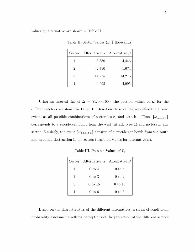
54
values by alternative are shown in Table II.
Table II. Sector Values (in $ thousands)
Sector Alternative α Alternative β
1 3,330 4,446
2 2,790 1,674
3 14,275 14,275
4 4,995 4,995
Using an interval size of ∆ = $1, 000, 000, the possible values of Li for the
different sectors are shown in Table III. Based on these values, we define the atomic
events as all possible combinations of sector losses and attacks. Thus, ω0,0,0,0,1
corresponds to a suicide car bomb from the west (attack type 1) and no loss in any
sector. Similarly, the event ω4,3,15,6,3 consists of a suicide car bomb from the south
and maximal destruction in all sectors (based on values for alternative α).
Table III. Possible Values of Li
Sector Alternative α Alternative β
1 0 to 4 0 to 5
2 0 to 3 0 to 2
3 0 to 15 0 to 15
4 0 to 6 0 to 6
Based on the characteristics of the different alternatives, a series of conditional
probability assessments reflects perceptions of the protection of the different sectors

55
by each alternative against the various attack types. These assessments are located
in Appendix A for alternative α and in Appendix B for alternative β.
The attack probability assessments (5.1)-(5.10) and the loss probability assess-
ments in the appendices are each then converted to constraints in terms of the atomic
events. We use the convention pijlmk = Pωi,j,l,m,k. Thus i corresponds to the mag-
nitude of loss in sector 1, j to loss in sector 2, l to loss in sector 3, m to loss in sector 4,
and k to the type of attack. Examples of assessments and corresponding constraints
are
Pα(Aα = 2) ≤ 0.3 ⇒∑ijlm
pαijlm2 ≤ 0.3
and
Pβ(Lβ1 = 0|Aβ = 1) ≤ 0.9 ⇒
∑jlm
0.1 pβ0jlm1 −
5∑i=1
∑jlm
0.9 pβijlm1 ≤ 0.
The final constraint for each alternative is the requirement that P (Ω) = 1 which
becomes ∑ijlmk
pijlmk = 1. (5.11)
The utility function used for the scenario was
u(x) = a + be−xρ , x ∈ [0, 28]
with a = 131.43685, b = −31.43685, and ρ = 18.87391658. This function is shown
plotted over the possible loss values in figure 4. This function returns a utility value of
100 for operation of the FOB with no losses, and a loss of $27 million, which exceeds
the value of the FOB with all its personnel and equipment, returns a utility value of

56
Fig. 4. Plot of Utility Function
zero. The objective function for the linear programs for alternative α thus becomes
c(pα) =∑ijlmk
[a + be(i+j+l+m)/ρ] pαijlmk
= a + b∑ijlmk
e(i+j+l+m)/ρ pαijlmk.
The objective function for alternative β is identical except that the decision variables
are given by the vector pβ.
The linear programs for the two alternatives were each coded using AMPL math-
ematical programming software and solved using the CPLEX solver.

57
E. Analysis of Results
As a result of solving each alternative’s formulation as both maximization and
minimization problems, the expected utility values were determined to be in the
interval [93.4667, 99.5059] for alternative α and in the interval [94.4837, 99.4554] for
alternative β. Since no separation exists between the intervals, a preference cannot be
determined for one alternative over the other with the current state of information.
However, examining the linear programming solutions provides insights regarding the
situation.
1. Insight from the Dual Solutions
The non-zero values for the dual variables from each of the solutions of the linear
programs are shown in Appendix D. Each value πc corresponds either to constraint c
in Appendix A or B (depending on the alternative being considered) or to constraints
(5.1)-(5.11). In Appendix D, these values are sorted by magnitude for each of the
optimization problems for each alternative.
a. Dual Values as Shadow Prices
The traditional interpretation of the dual variables as shadow prices for the right
hand side quantities applies here with respect only to constraints (5.1)-(5.10). The
right hand side of constraint (5.11) can never be changed, and the constraints in the
appendices are all based on conditional probabilities and will thus have a right hand
side value of zero.
For alternative α, the dual variables corresponding to constraints (5.3), (5.4),
and (5.6) are all non-zero for both the minimization and maximization problems.
Additionally, all have a negative value for the minimization problem and a positive

58
value for the maximization problem. Since each of these constraints is an upper
bound on an attack probability, tightening these upper bounds would potentially
tighten both the upper and lower bounds on expected utility. Given the choice of
which constraint to focus information gathering efforts on for alternative α, the officer
should choose either constraint (5.3) or (5.6) since the magnitudes of their dual values
are greater than those of constraint (5.4) in both the minimization and maximization
problems.
For alternative β, the dual variables for constraints (5.1), (5.3), and (5.6) are
non-zero for the minimization problem, and the dual variables for constraints (5.4),
(5.6), and (5.8) are non-zero for the maximization problem. Since the magnitude
of π5.6 is the largest of the three values in the minimization problem and since it is
the only constraint with non-zero values for both problems, the officer should focus
efforts on tightening constraint (5.6) to tighten the bounds on expected utility for
alternative β.
Given that the analysis of the dual variables for the attack probability constraints
for both alternatives point to tightening the upper bound on P (A = 4), the officer may
want to focus on gathering additional intelligence on the likelihood of a dismounted
attack from the north.
b. Shadow Pricing for Conditional Probabilities
Using Equation (4.6) to compute shadow prices for conditional probabilities is not
as straightforward as using the traditional interpretation of the dual variables. Several
factors must be considered. First, which of the constraints have a dual variable with
a large magnitudes? Second, what is the sense of the constraint that corresponds to
a large dual value? Is it an equality or an inequality? Third, for the current optimal
solution, what is the probability of the conditioning event for the constraint under

59
consideration? Once a shadow price is able to be computed, we may then turn to
the questions of whether the right hand side should be increased or decreased and
what must be done to justify such an adjustment in the mind of the officer. To show
the implications of each of these questions, we consider the minimization problem of
alternative α.
The constraints with the dual variable of the largest magnitude is constraint 52
with π52 = −59.5041. Constraint 52 is an equality constraint with a right hand side
value of one. In this scenario, constraints of this type serve the purpose of placing an
upper bound on the loss in a sector given that an attack occurs and that the loss in
the protective sector closest to the attack is not zero. The right hand side of this type
of constraint cannot be adjusted and still serve its purpose. In fact, in the probability
assessments used for this scenario, all of the equality constraints have a right hand
side of one and conditionally either place an upper bound on loss in a sector or fix
the loss in a sector at zero. Thus, we should limit the constraints under consideration
to those which are inequality constraints.
The inequality constraint with the dual value of highest magnitude is constraint
28 which is
Pα(Lα3 ≤ 1|Lα
2 > 0, Aα = 2) ≥ 0.8.
To compute the shadow price using Equation (4.6), we must compute the conditioning
event probability, Pα(Lα2 > 0, Aα = 2). In terms of the atomic event probabilities, we
see that
Pα(Lα2 > 0, Aα = 2) =
5∑j=1
∑ilm
pijlm2 = 0.09.
Before applying Equation (4.6) to compute the shadow price, we must consider that
this result was obtained from the linear program (4.5) which is a maximization prob-
lem while we are working with a minimization problem. Since the conversion from
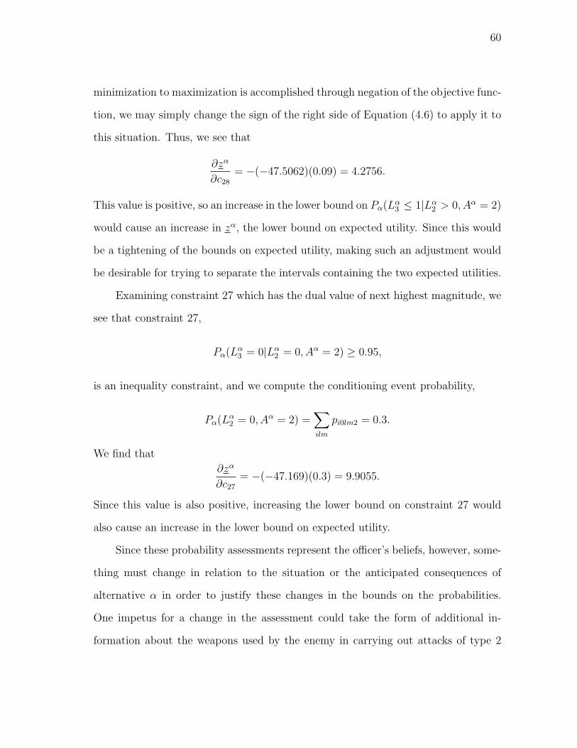
60
minimization to maximization is accomplished through negation of the objective func-
tion, we may simply change the sign of the right side of Equation (4.6) to apply it to
this situation. Thus, we see that
∂zα
∂c28
= −(−47.5062)(0.09) = 4.2756.
This value is positive, so an increase in the lower bound on Pα(Lα3 ≤ 1|Lα
2 > 0, Aα = 2)
would cause an increase in zα, the lower bound on expected utility. Since this would
be a tightening of the bounds on expected utility, making such an adjustment would
be desirable for trying to separate the intervals containing the two expected utilities.
Examining constraint 27 which has the dual value of next highest magnitude, we
see that constraint 27,
Pα(Lα3 = 0|Lα
2 = 0, Aα = 2) ≥ 0.95,
is an inequality constraint, and we compute the conditioning event probability,
Pα(Lα2 = 0, Aα = 2) =
∑ilm
pi0lm2 = 0.3.
We find that
∂zα
∂c27
= −(−47.169)(0.3) = 9.9055.
Since this value is also positive, increasing the lower bound on constraint 27 would
also cause an increase in the lower bound on expected utility.
Since these probability assessments represent the officer’s beliefs, however, some-
thing must change in relation to the situation or the anticipated consequences of
alternative α in order to justify these changes in the bounds on the probabilities.
One impetus for a change in the assessment could take the form of additional in-
formation about the weapons used by the enemy in carrying out attacks of type 2

61
(suicide bombings or improvised explosive devices). However, there is no guaran-
tee that such information would cause the probabilities to increase. The primary
matter that is under the control of the officer is the configuration, placement, and
construction of the positions in the sectors. What increasing the lower bound on
Pα(Lα3 = 0|Lα
2 = 0, Aα = 2) means, practically, is that the officer is more certain that
no damage will occur in sector 3 if an attack of type 2 occurs and no damage occurs
in sector 2. Increasing the lower bound on Pα(Lα3 ≤ 1|Lα
2 > 0, Aα = 2) would indicate
that, if damage in sector 2 occurs due to a type 2 attack, the officer is more certain
that a lower magnitude of loss would be incurred in sector 3. Since the location of a
type 2 attack is directly adjacent to sector 2, the decision maker can reduce the prob-
ability of such an attack affecting sector 3 by increasing the distance between sectors
2 and 3 or by constructing protective barriers between the sectors. Since this adds
another safeguard to the current configuration, the officer would in fact be creating
a new alternative and should consider whether the previous probability assessments
for other events are valid for the new alternative.
Rather than create a new alternative on the basis of the analysis of a limited
number of shadow prices, the officer should consider whether the implications of a
combination of shadow prices might produce a better alternative. In the problem
under consideration, the eight inequality constraints with the largest shadow price
values are shown in Table IV. Note that the partial derivatives with respect to the
right sides of these assessments are all positive.
Note that five of the eight constraints are assessments that involve loss in sector
3 and that the two highest partial derivative values are included in these five. This
is an indication that making the probability of damage to sector 3 as unlikely as
possible would increase the lower bound on expected utility. Additionally, since the
conditioning events in these assessments involve all of the other sectors in the FOB,

62
Table IV. Conditional Probability Constraint Shadow Prices
j Constraint j ∂zα/∂cj
63 Pα(Lα3 = 0|Lα
4 = 0, Aα = 4) ≥ 0.8 12.0206
27 Pα(Lα3 = 0|Lα
2 = 0, Aα = 2) ≥ 0.95 9.9055
17 Pα(Lα2 = 0|Aα = 2) ≥ 0.7 4.3069
28 Pα(Lα3 ≤ 1|Lα
2 > 0, Aα = 2) ≥ 0.8 4.2756
5 Pα(Lα2 = 0|Lα
1 = 0, Aα = 1) ≥ 0.95 3.3602
15 Pα(Lα3 ≤ 4|Lα
1 > 0, Aα = 1) ≥ 0.99 3.0048
7 Pα(Lα2 ≤ 1|Lα
1 > 0, Aα = 1) ≤ 0.9 2.9980
9 Pα(Lα3 = 0|Lα
1 = 0, Aα = 1) ≥ 0.95 2.8620
this is an indication that the possibility of placing some type of protective barrier
between sector 3 and the others should be explored. Such a barrier would practically
enclose sector 3. Since sector 3 contains the living and headquarters areas and since
those areas contain the most value due to the concentration of soldiers in those areas,
construction of hardened buildings or reinforcement of current facilities for these areas
should be considered.
This result corresponds to the intuitive notion of using more assets to protect
items or areas of higher value. However, this example shows how the analytical
technique presented can identify areas of high value which are left vulnerable. This
identification of vulnerabilities is of primary importance in the evaluation of security
system alternatives. This evaluation is fundamental in the identification of a most
preferred alternative.

63
2. Consistency and the Primal Solutions
Although other methods exist to determine consistency of probability assess-
ments, linear programming provides an automatic check for consistency through the
determination of feasibility. Additionally, an examination of the values of the primal
variables (that is, the atomic event probabilities) can provide insight into whether the
given probability assessment actually reflects one’s perception of the situation. The
non-zero variables from each of the primal solutions of the linear programs in this
scenario are shown in Appendix D. Each value for pijlmk in these tables represents a
probability which corresponds to an atomic event which, according to the probability
assessments, may have a non-zero probability and which contributes to either the
maximum or minimum value for expected utility for its respective alternative.
One consideration is whether the probabilities do, in fact, represent one’s beliefs
regarding the possible consequences of the alternative configuration for which they
were given. The probabilities in Table V are extracted from the solution for the
minimization problem for alternative α. Note that the value corresponding to the
index l is 15 for all of these events. Summing these probabilities, we see that for the
probability law corresponding to this solution,
PαLα3 = 15 = 0.097.
This indicates that the officer’s assessment of the situation allows for a probability
of almost 0.1 that the headquarters, living, and parking areas (sector 3) will be
destroyed. If the officer does not believe that the probability may be that high, he
should adjust the probability assessments to reflect this belief. If he does believe the
probability may be that high, he should consider adjusting the configuration so that
those key areas are better protected.

64
Table V. Probability of Destruction of Sector 3
i j l m k pijlmk
0 0 15 0 1 0.00375
0 0 15 0 4 0.063
0 0 15 5 3 0.001
2 3 15 0 1 0.00075
4 0 15 0 2 0.0105
4 1 15 0 2 0.018
Another consideration for the officer is whether events with non-zero probabilities
would actually occur. The first two lines in Table V correspond to events where an
attack occurs and none of the protective measures incurs any loss, yet the living area
is completely destroyed. The officer must consider whether or not he believes that
this could actually happen. If so, then, again, he should consider a modification to
the configuration to prevent such a catastrophic occurrence. If not, then he should
add constraints to reflect that belief. One possible constraint would be
Pα(Lα3 ≤ 7|Aα = 4) = 1
which would place a bound on the loss in sector 3 due to attack 4. An assessment
of this type will further constrain the feasible region and may also tighten the lower
bound on expected utility.
This chapter has presented an application of the analytical framework developed
in Chapter IV for identification of a preferred alternative under incomplete charac-
terization of probability law. A military scenario involving the security of a FOB was

65
considered as a special case of the physical security problem. Linear optimization
problems to find the bounds on expected utility for two alternatives were formulated
and solved. Results showed that, while neither alternative was preferred over the
other, an examination of the primal and dual solutions provided insight into three
primary areas:
• information that should be gathered to tighten the bounds on expected utility,
• identification of vulnerabilities in high-value areas, and
• consistency of probability assessments.

66
CHAPTER VI
CONCLUSION
This dissertation has accomplished the research objectives presented at the out-
set. The first objective was to identify an objective function for the physical security
system decision which orders preferences for the decision maker. In Chapter III,
the basis for the use of expected utility as the objective function was presented. In
Chapter IV, an objective function was derived which is a computation of expected
utility within the context of the problem examined. The second objective was to
determine conditions for the separation of preferences without complete characteri-
zation of probability law. In Chapter IV, we presented a method to determine upper
and lower bounds on expected utility through the use of linear programming. Sep-
aration of preferences occurs when the lower bound on utility for one alternative
exceeds the upper bound on utility for another. The third objective was to identify
insights available to the decision maker through interpretation of aspects of the model
structure. Chapter IV discussed sensitivity analysis methods available in linear pro-
gramming which are applicable to the formulation of the problem studied here. The
interpretation of the information provided through sensitivity analysis was illustrated
in Chapter V where we provided techniques to give insight both into vulnerabilities
that exist within a design and also into which threats merit additional information
gathering efforts.
In this final chapter, as an area for further research, we present an extension
of physical security system assessment to the case where neither the probability law
nor the utility function are uniquely specified. Finding bounds on expected utility
in this case can be accomplished via bilinear programming, and we give formulations
of these problems. Following the discussion of this research extension, we discuss

67
the motivation for considering this topic and give possible application areas for the
assessment framework.
A. Future Research Areas
In research on educating or training leaders in decision making, Cohen, Freeman,
and Thompson [64] present a descriptive model which identifies qualities and skills
of proficient decision makers and thus offers specific foci for training. Klein and
Wolf [49] include modeling the cognitive processes of subject-matter experts as one
of the primary guidelines for training decision makers. Thus, in training people to be
better decision makers, efforts are made to describe what characteristics and thought
processes a good decision maker possesses.
Applying this approach to training decision makers using an expected utility
paradigm, expert decision makers can be considered to have utility functions with
specific characteristics. In training people to make good decisions in specific situa-
tions, success could be measured by determining whether the utility function used by
the student is similar to that of an expert in that situation. One approach would be
to identify a range of utility functions that would be acceptable and then to determine
if the utility function used to make the decision falls within that range.
The model presented in Chapter IV can be extended to the case where a utility
function is not specified but is known to lie within certain boundaries. We show that
such an assessment problem may be modeled using bilinear programs which may be
solved to determine upper and lower bounds on expected utility for each alternative.
A separation of the bounds on expected utility serves to order preferences among
alternatives if such a separation exists.

68
1. Problem Description
The assessment situation is identical to that in Chapter IV except that the util-
ity function is not known. Instead, the utility function is required to lie between
certain boundaries. Some assets are to be protected, and alternative configurations
of safeguards have been identified with which to protect the assets. The assets to be
protected are partitioned into N sectors, and M possible types of threats have been
identified. For each alternative configuration, an assessment is made of the probabil-
ities of the occurrence of the attack types and of consequences of attacks, but these
probability assessments do not result in a unique probability law on reward for each
alternative.
As shown in (4.2), if a utility function u is given, the calculation of the expected
utility for alternative α is
Eα(U) =H∑
h=1
u(a + h∆)
∑(n,k)∈Nh
pα(n,k)
where
Nh = (n, k) : ‖n‖1 = −a− h∆, 1 ≤ k ≤ M.
However, in the problem under consideration, no utility function is given. We consider
two monotone, continuous functions uU : R → R and uL : R → R as boundaries on
the utility function. That is, we require that
uL(x) ≤ u(x) ≤ uU(x), x ∈ R.
An illustration of utility boundary functions is shown in Figure 5 where [a, b] is the
support of the risk distribution for alternative α. The plot of an acceptable utility
function would fall within the shaded region.

69
Fig. 5. Boundaries of a Utility Function
2. Formulation of Bilinear Programs
Considering the expression which we have derived for expected utility which we
used as an objective function in Chapter IV, we see that H evaluations of the utility
function are needed to determine a bound on expected utility. These are
u(a + h∆), h = 1, . . . , H.
Each of these evaluations may be considered to be a decision variable to which a value
must be assigned. Let
uh = u(a + h∆), h = 1, . . . , H.
Then for each uh, we have the following constraints:
uh ≥ uL(a + h∆)
uh ≤ uU(a + h∆).

70
Additionally, we require that the unknown utility function be monotone. Therefore,
we include the constraints
uh ≤ uh+1, h = 1, . . . , H − 1.
Let u = (u1, . . . , uH) be the vector of utility decision variables. Then the con-
straints on these decision variables can be expressed as
A1u ≥ b1.
Just as in Chapter IV, we denote the constraints on the probability decision variables
for alternative α ∈ A as
Aα2p
α ≥ bα2 .
The objective function which is simply the adjusted expression for expected utility
becomes
c(u,pα) =H∑
h=1
∑(n,k)∈Nh
uh pα(n,k).
Thus we have two bilinear programs for each alternative. The lower bound for
expected utility for alternative α is found by solving
zα = min c(u,pα)
s.t. A1u ≥ b1
Aα2p
α ≥ bα2 .
Similarly, the upper bound for expected utility for alternative α is found by solving
zα = max c(u,pα)
s.t. A1u ≥ b1
Aα2p
α ≥ bα2 .

71
These bilinear programs both have nonlinear objective functions and linear con-
straints. Problems of this type have been studied and various solution techniques
have been applied with success. Al-Khayyal [65] gives a thorough overview of related
problems and a survey of solution methodologies.
For two alternatives α, β ∈ A, a preference for one alternative over another can
be determined whenever zα > zβ or zβ > zα. Thus, in certain instances, it is possible
determine a preference between alternatives when neither the probability law nor the
utility function is precisely specified.
B. Concluding Remarks
In this conclusion, we first comment on the motivation and performance of the
research presented in this dissertation. We close with a discussion of other potential
application areas for our analytical framework.
1. Motivation and Flow of Research
The initial motivation for this research was to develop an analytical framework
which could be used in to educate and train current and future Army officers in
decision making. The focus was on providing an analytical framework which could be
used to develop decision scenarios to allow future Army leaders to better understand
uncertainty, to discover aspects of their own decision styles and preferences, and to
develop a sense of consistency. The need for improved education in decision making
for Army officers was recognized by General (Retired) Montgomery Meigs in the
spring of 2001, prior to the attacks of September 11 and America’s entry into the
Global War on Terror:

72
Among staff college students and about-to-be general officers as well, we
must foster a better understanding of the uncertainty inherent in opera-
tions and the processes by which they can best deal with that uncertainty.
Our professional education must engender better decisionmaking by fur-
nishing the intellectual tools that bolster leaders against stress, friction,
and fog, and against the pressures of their fears and those of their political
masters....In this regard we need a very sophisticated course of hands-on
case studies in how decisions are enabled and made, not just the study of
staff duties and political science in a military context. [66]
The desire was to provide a tool to enable the training of officers in tough, realistic,
ambiguous, combat-related decision scenarios so that making decisions under these
conditions would not be as difficult in actual combat situations.
As research into the problem continued, it became evident that the need for deci-
sion making education in the security arena was not limited to the Army. Certainly,
other branches of the military would benefit from decision education of this sort.
However, the challenges facing decision makers in Homeland Security, port security,
stadium security, and many other areas would indicate that decision making skills in
the security sector are absolutely necessary due to the high price of failure. Thus,
the focus of the research broadened, and the military decision scenario was seen to
be a special case of the more general physical security decision problem. Since such
a decision is a matter of choosing the alternative with the preferred risk, the need to
focus on security risk assessment became apparent.

73
2. Further Areas for Application
The analytical framework that was developed in this research was applied to a
military scenario where Army forces are securing a FOB, and a decision maker must
decide between alternative configurations of forces. In the scenario presented, the
decision maker is concerned with a small area and a limited number of forces. The
technique presented, however, has applications across the military services and across
the spectrum of force levels. Consider the deployment of a carrier strike group in
the U.S. Navy. A carrier strike group consists of an air craft carrier and a mission-
dependent combination of guided missile cruisers, guided missile destroyers, attack
submarines, and a combat support ship for logistical support. [67] The group com-
mander has the responsibility to protect the aircraft carrier and the other ships in
the strike group using the assets that comprise the group. He must consider the
threats to the group and array the ships and aircraft coverage to counter the threats
appropriately while simultaneously performing the group’s mission. While an Army
lieutenant or captain might oversee the security of a small FOB, a Navy rear admiral
is ultimately responsible for the security of a carrier strike group. Other possible
scenarios include the securing of a beachhead by U.S. Marines or the protection of
an air base by security forces of the Air Force. The flexibility of the framework in
military applications is evident.
Because of this flexibility in the application of the analytical framework, numer-
ous opportunities exist for employing the framework in the education and training of
military decision makers. One potential application would be to use decision scenarios
to provide feedback on consistency in both decision making and threat assessment.
Military leaders must be able to act in accordance with their values and their under-
standing of the situation at hand. An understanding of consistency and practice in

74
facing ambiguous decision scenarios will enable leaders to make decisions when facing
real life situations in the so-called “fog of war”. Another application is the employ-
ment of the model to identify weaknesses in plans and decisions under uncertainty
in training scenarios. Using the capability within the framework to identify potential
vulnerabilities, officers can learn to develop thorough plans and to see when resource
constraints leave missions or facilities exposed to unacceptable levels of loss of life or
equipment. Through the development of applications such as these, valuable experi-
ence in making hard decisions under combat-related conditions of uncertainty can be
gained.
Potential applications for the framework in educating security decision makers
exist outside of the military domain as well. Border and port security are prime
examples of situations where a fixed asset must be protected by arranging sets of
safeguards in response to uncertain threats. Not only are the threats uncertain, they
are manifold due to the amount of traffic and cargo that passes through these types
of facilities. Officials in these areas must be well versed in the consideration of threat
information and the proper response to such information. Moreover, the ability to
determine which threats warrant the pursuit of additional information would be of
value due to the large number of potential threats faced by border and port security
systems. The framework presented here can assist in providing this ability.

75
REFERENCES
[1] K. M. Kenyon, Digging Up Jericho, Frederick A. Praeger, New York, 1957.
[2] R. J. Fischer and G. Green, Introduction to Security, 7th Edition, Elsevier,
Boston, 2004.
[3] ASIS International, “ASIS International launches two additional professional
certification programs,” 2002, [Online]. Available: http://www.asisonline.org/
newsroom/pressReleases/120902certs.xml, accessed April 27, 2006.
[4] I. Horrocks, “Security training: Education for an emerging profession?,” Com-
puters & Security, vol. 20, pp. 219–226, 2001.
[5] ASIS International, “Academic institutions offering degrees and/or courses
in security,” 2006, [Online]. Available: http://www.asisonline.org/education/
universityPrograms/traditionalprograms.pdf, accessed April 27, 2006.
[6] Sandia National Laboratories, “A risk assessment methodology (RAM) for phys-
ical security,” White Paper, 2006, [Online]. Available: http://www.sandia.gov/
ram/RAM%20White%20Paper.pdf, accessed April 27, 2006.
[7] Department of the Army, Physical Security, Field Manual 3-19.30, Government
Printing Office, Washington, D.C., Jan 2001.
[8] M. L. Garcia, The Design and Evaluation of Physical Protection Systems,
Butterworth–Heinemann: Boston, 2001.
[9] S. Kaplan and B. J. Garrick, “On the quantitative definition of risk,” Risk
Analysis, vol. 1, no. 1, pp. 11–27, 1981.

76
[10] S. Scandizzo, “Risk mapping and key risk indicators in operational risk manage-
ment,” Economic Notes, vol. 34, no. 2, pp. 231–256, 2005.
[11] K. Smith, C. B. Barrett, and P. W. Box, “Participatory risk mapping for target-
ing research and assistance: With an example from east African pastoralists,”
World Development, vol. 28, no. 11, pp. 1945–1959, 2000.
[12] M.A. Wortman and J. H. Park, “Decisions in engineering design: Separat-
ing preferences via distribution families,” Working Paper, 2004, Department
of Industrial and Systems Engineering, Texas A&M University, College Station,
Texas.
[13] M. J. Hicks, M. S. Snell, J. S. Sandoval, and C. S. Potter, “Cost and perfor-
mance analysis of physical protection systems–a case study,” in Proceedings
32nd Annual 1998 International Carnahan Conference on Security Technology,
Alexandria, Virginia, 1998, pp. 79–84.
[14] L. R. Doyon, “Stochastic modeling of facility security-systems for analytical
solutions,” Computers & Industrial Engineering, vol. 5, no. 2, pp. 127–138,
1981.
[15] W. J. Schneider and R. P. Grassie, “Countermeasures development in the
physical security design process: an anti-terrorist perspective,” in Proceedings
IEEE 1989 International Carnahan Conference on Security Technology, Zurich,
Switzerland, 1989, pp. 297–302.
[16] R. P. Grassie, A. J. Johnson, and W. J. Schneider, “Countermeasures selection
and integration: a delicate balancing act for the security designer,” in Pro-
ceedings IEEE 1990 International Carnahan Conference on Security Technology:
Crime Countermeasures, Lexington, Kentucky, 1990, pp. 116–123.

77
[17] J. E. Kobza and S. H. Jacobson, “Probability models for access security system
architectures,” The Journal of the Operational Research Society, vol. 48, no. 3,
pp. 255–263, Mar 1997.
[18] S. H. Jacobson, J. E. Kobza, and A. S. Easterling, “A detection theoretic ap-
proach to modeling aviation security problems using the knapsack problem,” IIE
Transactions, vol. 33, no. 9, pp. 747–759, Sep 2001.
[19] V. M. Bier and V. Abhichandani, “Optimal allocation of resources for defense of
simple series and parallel systems from determined adversaries,” in Proceedings
of Risk-Based Decisionmaking in Water Resources X, Y. Y. Haimes, D. A. Moser,
and E. Z. Stakhiv, Eds., Santa Barbara, California, 2002, vol. 129, pp. 59–76,
American Society of Civil Engineers.
[20] J. Sher and C. Guryan, “Network optimization methods for terrorism vulnera-
bility assessment,” Presented at the 71st Military Operations Research Society
Symposium, Quantico, Virginia, Jun 2003.
[21] G. G. Wagner, “Design process of physical security as applied to a U.S. Border
Port of Entry,” in Proceedings SPIE Conference on Enforcement and Security
Technologies, A. T. DePersia and J. J. Pennella, Eds., Boston, Massachusetts,
1998, vol. 3575, pp. 182–188.
[22] E. E. Hinman and D. J. Hammond, Lessons From the Oklahoma City Bombing:
Defensive Design Techniques, American Society of Civil Engineers, New York,
1997.
[23] L. Peck, “Weather and terrain effects on electronic security systems: Impact on
force protection command decisions,” Presented at the 69th Military Operations
Research Society Symposium, Annapolis, Maryland, Jun 2001.

78
[24] L. Peck, “Ensuring effective sensor-based intrusion detection at base camps,”
Presented at the 3rd Base Camp Workshop, West Point, New York, May 2005.
[25] L. Peck and J. Lacombe, “Sensor-based base camp security,” in Proceedings
SPIE Conference on Unattended/Unmanned Ground, Ocean, and Air Sensor
Technologies and Applications VI, E. M. Carapezza, Ed., Orlando, Florida, 2004,
pp. 364–369.
[26] A. Cowdale and S. Lithgo, “Planning aids for the military commander: Force
protection simulation opportunities with GIS,” in Proceedings of the 2001 Win-
ter Simulation Conference, B.A. Peters, J.S. Smith, D.J. Medeiros, and M.W.
Rohrer, Eds., Arlington, Virginia, 2001, pp. 680–683.
[27] J. von Neumann and O. Morgenstern, Theory of Games and Economic Behavior,
Princeton University Press, Princeton, New Jersey, 2004.
[28] L. J. Savage, The Foundations of Statistics, 2nd Revised Edition, Dover, New
York, 1972.
[29] I. J. Good, “Rational decisions,” Journal of the Royal Statistical Society. Series
B., vol. 14, no. 1, pp. 107–114, 1952.
[30] I. J. Good, “The appropriate mathematical tools for describing and measur-
ing uncertainty,” in Uncertainty and Business Decisions, C. F. Carter, G. P.
Meredith and G. L. S. Shackle, Eds., The University Press of Liverpool, United
Kingdom, 1954, pp. 19–34.
[31] C. A. B. Smith, “Consistency in statistical inference and decision,” Journal of
the Royal Statistical Society. Series B., vol. 23, no. 1, pp. 1–37, 1961.

79
[32] P. C. Fishburn, The Foundations of Expected Utility, D. Reidel Publishing
Company, Dordrecht, The Netherlands, 1982.
[33] J. Y. Halpern, Reasoning about Uncertainty, The MIT Press, Cambridge,
Massachusetts, 2003.
[34] P. C. Fishburn, Decision and Value Theory, Number 10 in Publications in
Operations Research. John Wiley & Sons, New York, 1964.
[35] P. C. Fishburn, “Analysis of decisions with incomplete knowledge of probabili-
ties,” Operations Research, vol. 13, no. 2, pp. 217–237, Mar-Apr 1965.
[36] P. C. Fishburn, A. H. Murphy, and H. H. Isaacs, “Sensitivity of decisions to
probability estimation errors: A reexamination,” Operations Research, vol. 16,
no. 2, pp. 254–267, Mar–Apr 1968.
[37] C. C. White, “A survey on the integration of decision analysis and expert systems
for decision support,” IEEE Transactions on Systems, Man, and Cybernetics,
vol. 20, no. 2, pp. 358–364, Mar–Apr 1990.
[38] R. R. Yager and V. Kreinovich, “Decision making under interval probabilities,”
International Journal of Approximate Reasoning, vol. 22, pp. 195–215, 1999.
[39] M. Danielson and L. Ekenberg, “A framework for analysing decisions under
risk,” European Journal of Operational Research, vol. 104, no. 3, pp. 474–484,
1998.
[40] J. E. Bickel and J. E. Smith, “Optimal sequential exploration,” Decision Anal-
ysis, vol. 3, no. 1, pp. 16–32, Mar 2006.
[41] E. T. Jaynes, “Information theory and statistical mechanics,” Physical Review,
vol. 106, no. 4, pp. 620–630, May 1957.

80
[42] E. T. Jaynes, “On the rationale of maximum-entropy methods,” Proceedings of
the IEEE, vol. 70, no. 9, pp. 939–952, Sep 1982.
[43] A. E. Abbas, “Entropy methods for joint distributions in decision analysis,”
IEEE Transactions on Engineering Management, vol. 53, no. 1, pp. 146–159, Feb
2006.
[44] I. J. Good, “Maximum entropy for hypothesis formulation, especially for mul-
tidimensional contingency tables,” The Annals of Mathematical Statistics, vol.
34, no. 3, pp. 911–934, Sep 1963.
[45] D. G. Lowell, “Examining sensitivity to relevance in decision analysis,” in
The Foundations of Professional Decision Analysis: A Collection of Readings.
Strategic Decisions Group, Palo Alto, California, Aug 1996.
[46] S. F. Barnett, “Computer security training and education: A needs analysis,”
in Proceedings of the 1996 IEEE Symposium on Security and Privacy (SP ’96),
Oakland, California, 1996, pp. 26–27.
[47] R. Martin, “NGO field security,” Forced Migration Review, vol. 4, pp. 4–7, Apr
1999.
[48] K. Van Brabant, “Security training: where are we now?,” Forced Migration
Review, vol. 4, pp. 7–10, Apr 1999.
[49] G. Klein and S. Wolf, “Decision-centered training,” in Proceedings of the Human
Factors and Ergonomics Society 39th Annual Meeting, San Diego, California,
1995, pp. 1242–1252.
[50] E. S. Tzannatos, “A decision support system for the promotion of security in
shipping,” Disaster Prevention and Management, vol. 12, no. 3, pp. 222–229,

81
2003.
[51] V. Baron and N. van Zwanenberg, “Decision making in the provision of security
services,” Facilities, vol. 14, no. 1/2, pp. 9–16, Jan/Feb 1996.
[52] P. C. Fishburn, “Retrospective on the utility theory of von Neumann and Mor-
genstern,” Journal of Risk and Uncertainty, vol. 2, no. 2, pp. 127–157, Jun
1989.
[53] C. Puppe, Distorted Probabilities and Choice Under Risk, Number 363 in
Lecture Notes in Economics and Mathematical Systems. Springer–Verlag, New
York, 1991.
[54] D. Williams, Probability with Martingales, Cambridge University Press, Cam-
bridge, 1991.
[55] J.M. Hampton, P.G. Moore, and H. Thomas, “Subjective probability and its
measurement,” Journal of the Royal Statistical Society. Series A (General), vol.
136, no. 1, pp. 21–42, 1973.
[56] M. S. Bazaraa, J. J. Jarvis, and H. D. Sherali, Linear Programming and Network
Flows, 2nd Edition, John Wiley & Sons, New York, 1990.
[57] R. M. Freund, “The sensitivity of a linear program solution to changes in ma-
trix coefficients,” Sloan Working Paper No. 1532-84, Massachusetts Institute of
Technology, Cambridge, Massachusetts, Feb 1984.
[58] R. M. Freund, “Postoptimal analysis of a linear program under simultaneous
changes in matrix coefficients,” Mathematical Programming Study, vol. 24, 1985.

82
[59] Department of Defense, Department of Defense Dictionary of Military and Asso-
ciated Terms, Joint Publication 1-02, Government Printing Office, Washington,
D.C., Apr 2001, As Amended Through 9 May 2005.
[60] Department of Systems Engineering, “Base camp construction planning decision
support tool (DST),” Tech. Rep., United States Military Academy, West Point,
New York, Jun 2005.
[61] D. L. Thomas II, “The U.S. Army: A business? Return on investment?,”
2004, [Online]. Available: http://www.military.com/NewContent/0,13190,
120304 ArmyBusiness-P1,00.html, accessed April 5, 2006.
[62] Department of the Army, “Servicemembers Group Life Insurance,” 2005, [On-
line]. Available: https://www.hrc.army.mil/SITE/RESERVE/soldierservices/
pay/sglioverview.htm, accessed April 5, 2006.
[63] Military Advantage, “Fallen Hero Compensation,” 2006, [Online].
Available: http://www.military.com/Resources/ResourcesContent/0,13964,
30873-mil status active-1,00.html, accessed April 5, 2006.
[64] M. S. Cohen, J. T. Freeman, and B. B. Thompson, “Critical thinking skills in
tactical decision making: A model and a training method”, in Decision-Making
Under Stress: Implications for Training & Simulation, J. Canon-Bowers and E.
Salas, Eds., APA Press, Washington, D.C., 1998, pp. 155–189.
[65] F. A. Al-Khayyal, “Jointly constrained bilinear programs and related problems:
An overview,” Computers & Mathematics with Applications, vol. 19, no. 11, pp.
53–62, 1990.
83
[66] M. C. Meigs, “Operational art in the new century,” Parameters, vol. XXXI, no.
1, pp. 4–14, Spring 2001.
[67] Department of the Navy, “The Carrier Strike Group,” 2006, [Online]. Avail-
able: http://www.chinfo.navy.mil/navpalib/ships/carriers/powerhouse/cvbg.
html, accessed May 15, 2006.
[68] Department of the Navy, “United States Marine Corps Fact Files,”
2006, [Online]. Available: http://www.hqmc.usmc.mil/factfile.nsf/AVE?
openview&count=3000, accessed April 5, 2006.

84
APPENDIX A
PROBABILITY ASSESSMENTS FOR ALTERNATIVE α
The following are the probability assessments for loss under alternative α. The num-
bers to the right of each line correspond to the constraint numbers and thus dual
variable indices for those assessments.
Assessments for Attack Type 1
0.1 ≤ Pα(Lα1 = 0|Aα = 1) ≤ 0.6 (1, 2)
0.7 ≤ Pα(Lα1 ≤ 1|Aα = 1) (3)
Pα(Lα1 ≤ 2|Aα = 1) = 1 (4)
0.95 ≤ Pα(Lα2 = 0|Lα
1 = 0, Aα = 1) (5)
0.5 ≤ Pα(Lα2 ≤ 1|Lα
1 > 0, Aα = 1) ≤ 0.9 (6, 7)
0.95 ≤ Pα(Lα2 ≤ 2|Lα
1 > 0, Aα = 1) (8)
0.95 ≤ Pα(Lα3 = 0|Lα
1 = 0, Aα = 1) (9)
0.5 ≤ Pα(Lα3 ≤ 1|Lα
1 > 0, Aα = 1) ≤ 0.8 (10, 11)
0.7 ≤ Pα(Lα3 ≤ 2|Lα
1 > 0, Aα = 1) ≤ 0.95 (12, 13)
0.9 ≤ Pα(Lα3 ≤ 3|Lα
1 > 0, Aα = 1) (14)
0.99 ≤ Pα(Lα3 ≤ 4|Lα
1 > 0, Aα = 1) (15)
Pα(Lα4 = 0|Aα = 1) = 1 (16)

85
Assessments for Attack Type 2
0.7 ≤ Pα(Lα2 = 0|Aα = 2) ≤ 0.9 (17, 18)
0.85 ≤ Pα(Lα2 ≤ 1|Aα = 2) (19)
0.9 ≤ Pα(Lα2 ≤ 2|Aα = 2) (20)
0.9 ≤ Pα(Lα1 = 0|Lα
2 = 0, Aα = 2) (21)
0.6 ≤ Pα(Lα1 ≤ 1|Lα
2 > 0, Aα = 2) ≤ 0.9 (22, 23)
0.2 ≤ Pα(Lα1 ≤ 1|Lα
2 > 1, Aα = 2) ≤ 0.7 (24, 25)
Pα(Lα1 ≤ 2|Lα
2 > 1, Aα = 2) = 1 (26)
0.95 ≤ Pα(Lα3 = 0|Lα
2 = 0, Aα = 2) (27)
0.8 ≤ Pα(Lα3 ≤ 1|Lα
2 > 0, Aα = 2) (28)
0.1 ≤ Pα(Lα3 ≤ 1|Lα
2 > 1, Aα = 2) ≤ 0.5 (29, 30)
0.3 ≤ Pα(Lα3 ≤ 2|Lα
2 > 1, Aα = 2) ≤ 0.7 (31, 32)
0.6 ≤ Pα(Lα3 ≤ 3|Lα
2 > 1, Aα = 2) ≤ 0.9 (33, 34)
0.7 ≤ Pα(Lα3 ≤ 4|Lα
2 > 1, Aα = 2) ≤ 0.95 (35, 36)
0.8 ≤ Pα(Lα3 ≤ 5|Lα
2 > 1, Aα = 2) (37)
Pα(Lα3 ≤ 6|Lα
2 > 1, Aα = 2) = 1 (38)
Pα(Lα4 = 0|Aα = 2) = 1 (39)

86
Assessments for Attack Type 3
0.1 ≤ Pα(Lα1 = 0|Aα = 3) ≤ 0.6 (40, 41)
0.7 ≤ Pα(Lα1 ≤ 1|Aα = 3) (42)
Pα(Lα1 ≤ 2|Aα = 3) = 1 (43)
0.95 ≤ Pα(Lα4 = 0|Lα
1 = 0, Aα = 3) (44)
0.7 ≤ Pα(Lα4 ≤ 1|Lα
1 > 0, Aα = 3) ≤ 0.95 (45, 46)
Pα(Lα4 ≤ 2|Lα
1 > 0, Aα = 3) = 1 (47)
0.95 ≤ Pα(Lα3 = 0|Lα
1 = 0, Aα = 3) (48)
0.85 ≤ Pα(Lα3 = 0|Lα
1 > 0, Aα = 3) ≤ 0.95 (49, 50)
0.9 ≤ Pα(Lα3 ≤ 1|Lα
1 > 0, Aα = 3) (51)
Pα(Lα3 ≤ 2|Lα
1 > 0, Aα = 3) = 1 (52)
Pα(Lα2 = 0|Aα = 3) = 1 (53)
Assessments for Attack Type 4
0.7 ≤ Pα(Lα4 = 0|Aα = 4) ≤ 0.9 (54, 55)
0.8 ≤ Pα(Lα4 ≤ 1|Aα = 4) ≤ 0.95 (56, 57)
0.95 ≤ Pα(Lα4 ≤ 2|Aα = 4) (58)
0.99 ≤ Pα(Lα4 ≤ 3|Aα = 4) (59)
Pα(Lα4 ≤ 4|Aα = 4) = 1 (60)
Pα(Lα1 = 0|Aα = 4) = 1 (61)
Pα(Lα2 = 0|Aα = 4) = 1 (62)
0.8 ≤ Pα(Lα3 = 0|Lα
4 = 0, Aα = 4) (63)
0.75 ≤ Pα(Lα3 = 0|Lα
4 > 0, Aα = 4) ≤ 0.9 (64, 65)
0.95 ≤ Pα(Lα3 ≤ 1|Lα
4 > 0, Aα = 4) ≤ 0.99 (66, 67)
0.99 ≤ Pα(Lα3 ≤ 2|Lα
4 > 0, Aα = 4) (68)
Pα(Lα3 ≤ 5|Lα
4 > 0, Aα = 4) = 1 (69)
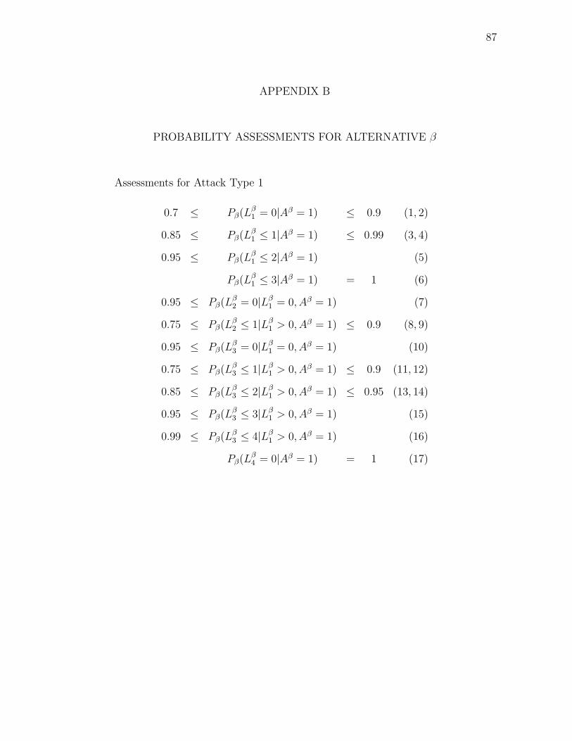
87
APPENDIX B
PROBABILITY ASSESSMENTS FOR ALTERNATIVE β
Assessments for Attack Type 1
0.7 ≤ Pβ(Lβ1 = 0|Aβ = 1) ≤ 0.9 (1, 2)
0.85 ≤ Pβ(Lβ1 ≤ 1|Aβ = 1) ≤ 0.99 (3, 4)
0.95 ≤ Pβ(Lβ1 ≤ 2|Aβ = 1) (5)
Pβ(Lβ1 ≤ 3|Aβ = 1) = 1 (6)
0.95 ≤ Pβ(Lβ2 = 0|Lβ
1 = 0, Aβ = 1) (7)
0.75 ≤ Pβ(Lβ2 ≤ 1|Lβ
1 > 0, Aβ = 1) ≤ 0.9 (8, 9)
0.95 ≤ Pβ(Lβ3 = 0|Lβ
1 = 0, Aβ = 1) (10)
0.75 ≤ Pβ(Lβ3 ≤ 1|Lβ
1 > 0, Aβ = 1) ≤ 0.9 (11, 12)
0.85 ≤ Pβ(Lβ3 ≤ 2|Lβ
1 > 0, Aβ = 1) ≤ 0.95 (13, 14)
0.95 ≤ Pβ(Lβ3 ≤ 3|Lβ
1 > 0, Aβ = 1) (15)
0.99 ≤ Pβ(Lβ3 ≤ 4|Lβ
1 > 0, Aβ = 1) (16)
Pβ(Lβ4 = 0|Aβ = 1) = 1 (17)

88
Assessments for Attack Type 2
0.5 ≤ Pβ(Lβ2 = 0|Aβ = 2) ≤ 0.8 (18, 19)
0.75 ≤ Pβ(Lβ2 ≤ 1|Aβ = 2) ≤ 0.95 (20, 21)
0.95 ≤ Pβ(Lβ1 = 0|Lβ
2 = 0, Aβ = 2) (22)
0.75 ≤ Pβ(Lβ1 ≤ 1|Lβ
2 > 0, Aβ = 2) ≤ 0.9 (23, 24)
0.85 ≤ Pβ(Lβ1 ≤ 2|Lβ
2 > 0, Aβ = 2) ≤ 0.99 (25, 26)
Pβ(Lβ1 ≤ 3|Lβ
2 > 0, Aβ = 2) = 1 (27)
0.95 ≤ Pβ(Lβ3 = 0|Lβ
2 = 0, Aβ = 2) (28)
0.8 ≤ Pβ(Lβ3 ≤ 1|Lβ
2 > 0, Aβ = 2) ≤ 0.95 (29, 30)
0.9 ≤ Pβ(Lβ3 ≤ 2|Lβ
2 > 0, Aβ = 2) (31)
0.95 ≤ Pβ(Lβ3 ≤ 3|Lβ
2 > 0, Aβ = 2) (32)
0.99 ≤ Pβ(Lβ3 ≤ 4|Lβ
2 > 0, Aβ = 2) (33)
0.2 ≤ Pβ(Lβ3 ≤ 1|Lβ
2 = 2, Aβ = 2) ≤ 0.5 (34, 35)
0.4 ≤ Pβ(Lβ3 ≤ 2|Lβ
2 = 2, Aβ = 2) ≤ 0.7 (36, 37)
0.6 ≤ Pβ(Lβ3 ≤ 3|Lβ
2 = 2, Aβ = 2) ≤ 0.9 (38, 39)
0.7 ≤ Pβ(Lβ3 ≤ 4|Lβ
2 = 2, Aβ = 2) ≤ 0.95 (40, 41)
0.8 ≤ Pβ(Lβ3 ≤ 5|Lβ
2 = 2, Aβ = 2) (42)
0.9 ≤ Pβ(Lβ3 ≤ 6|Lβ
2 = 2, Aβ = 2) (43)
0.99 ≤ Pβ(Lβ3 ≤ 7|Lβ
2 = 2, Aβ = 2) (44)
Pβ(Lβ4 = 0|Aβ = 2) = 1 (45)

89
Assessments for Attack Type 3
0.7 ≤ Pβ(Lβ1 = 0|Aβ = 3) ≤ 0.9 (46, 47)
0.85 ≤ Pβ(Lβ1 ≤ 1|Aβ = 3) ≤ 0.99 (48, 49)
0.95 ≤ Pβ(Lβ1 ≤ 2|Aβ = 3) (50)
Pβ(Lβ1 ≤ 3|Aβ = 3) = 1 (51)
0.99 ≤ Pβ(Lβ4 = 0|Lβ
1 = 0, Aβ = 3) (52)
0.7 ≤ Pβ(Lβ4 ≤ 1|Lβ
1 > 0, Aβ = 3) ≤ 0.95 (53, 54)
Pβ(Lβ4 ≤ 2|Lβ
1 > 0, Aβ = 3) = 1 (55)
0.99 ≤ Pβ(Lβ3 = 0|Lβ
1 = 0, Aβ = 3) (56)
0.9 ≤ Pβ(Lβ3 = 0|Lβ
1 > 0, Aβ = 3) ≤ 0.99 (57, 58)
0.95 ≤ Pβ(Lβ3 ≤ 1|Lβ
1 > 0, Aβ = 3) (59)
Pβ(Lβ3 ≤ 2|Lβ
1 > 0, Aβ = 3) = 1 (60)
Pβ(Lβ2 = 0|Aβ = 3) = 1 (61)

90
Assessments for Attack Type 4
0.7 ≤ Pβ(Lβ4 = 0|Aβ = 4) ≤ 0.9 (62, 63)
0.8 ≤ Pβ(Lβ4 ≤ 1|Aβ = 4) ≤ 0.95 (64, 65)
0.95 ≤ Pβ(Lβ4 ≤ 2|Aβ = 4) (66)
0.99 ≤ Pβ(Lβ4 ≤ 3|Aβ = 4) (67)
Pβ(Lβ4 ≤ 4|Aβ = 4) = 1 (68)
Pβ(Lβ1 = 0|Aβ = 4) = 1 (69)
Pβ(Lβ2 = 0|Aβ = 4) = 1 (70)
0.8 ≤ Pβ(Lβ3 = 0|Lβ
4 = 0, Aβ = 4) (71)
0.75 ≤ Pβ(Lβ3 = 0|Lβ
4 > 0, Aβ = 4) ≤ 0.9 (72, 73)
0.95 ≤ Pβ(Lβ3 ≤ 1|Lβ
4 > 0, Aβ = 4) ≤ 0.99 (74, 75)
0.99 ≤ Pβ(Lβ3 ≤ 2|Lβ
4 > 0, Aβ = 4) (76)
Pβ(Lβ3 ≤ 5|Lβ
4 > 0, Aβ = 4) = 1 (77)

91
APPENDIX C
EQUIPMENT VALUES
Equipment Value [68]
M16 Rifle $1,200
M2 .50 Caliber Machine Gun $14,000
M60 7.62mm Machine Gun $6,000
AT4 Light Anti-Armor Weapon $1,500
AN/PVS-4 Individual Weapon Night Sight $4,800
AN/TVS-5 Crew Served Weapon Night Sight $4,000
High Mobility Multipurpose Wheeled Vehicle (HMMWV) $75,0001
1The value of the M998 variant is $50,000. This variant includes no armor plating. An additional $25,000was added to the value to account for armor plating and communications equipment.

92
APPENDIX D
LINEAR PROGRAMMING RESULTS
Alternative α Minimization Primal Solution
i j l m k pαijlmk i j l m k pα
ijlmk
0 0 0 0 1 0.07125 1 0 0 1 3 0.12
0 0 0 0 2 0.189 2 0 1 0 1 0.0075
0 0 0 0 3 0.019 2 0 2 0 1 0.015
0 0 0 0 4 0.252 2 0 3 0 1 0.015
0 0 15 0 1 0.00375 2 2 4 0 1 0.00375
0 0 15 0 4 0.063 2 3 4 0 1 0.003
0 0 0 2 4 0.0175 2 3 15 0 1 0.00075
0 0 0 3 4 0.00875 2 0 0 1 3 0.006
0 0 1 3 4 0.00525 2 0 0 2 3 0.027
0 0 1 4 4 0.00175 2 0 1 2 3 0.009
0 0 2 4 4 0.0014 2 0 2 2 3 0.018
0 0 5 4 4 0.00035 4 0 0 0 2 0.0105
0 0 15 5 3 0.001 4 0 15 0 2 0.0105
1 0 1 0 1 0.03 4 1 1 0 2 0.018
1 1 1 0 2 0.054 4 1 15 0 2 0.018

93
Alternative α Minimization Dual Solution
c πc c πc
52 -59.5041 22 -6.34895
28 -47.5062 43 -4.82928
27 -47.1690 55 -3.43077
69 -46.7866 60 -2.75566
5 -44.8021 5.3 -2.68875
15 -40.0634 5.6 -2.68662
7 -39.9728 8 -2.61346
9 -38.1606 14 -2.22938
48 -38.1606 51 -2.22938
63 -38.1606 66 -2.22938
16 -27.5136 12 -2.11434
39 -27.5136 49 -2.11434
44 -21.1104 59 -2.11434
38 -16.6252 10 -2.00523
61 -16.4295 45 -2.00523
53 -15.6270 64 -2.00523
62 -14.8206 3 -1.90175
17 -14.3562 42 -1.90175
4 -13.2153 58 -1.90175
47 -8.2747 40 -1.69226
30 -8.2391 26 -0.70971
68 -7.4427 5.4 -0.33845
21 -7.4211 5.11 95.28130

94
Alternative α Maximization Primal Solution
i j l m k pαijlmk
0 0 0 0 1 0.09
0 0 0 0 2 0.27
0 0 0 0 3 0.12
0 0 0 0 4 0.315
0 1 0 0 2 0.027
0 0 0 1 4 0.014
0 0 1 1 4 0.00315
0 0 2 1 4 0.00035
0 0 0 2 4 0.0175
1 0 0 0 1 0.042
1 0 0 0 3 0.072
1 0 1 0 3 0.004
1 0 2 0 1 0.009
1 0 3 0 1 0.003
1 2 0 0 1 0.006
1 0 0 2 3 0.004
2 1 0 0 2 0.003

95
Alternative α Maximization Dual Solution
c πc
5.11 98.831000
7 3.705360
11 3.705360
23 3.705360
46 3.705360
2 2.922410
18 2.081080
13 2.005230
41 1.985990
55 1.909920
67 1.901750
50 1.803610
57 1.803610
65 1.803610
5.3 0.960856
5.6 0.887791
5.4 0.374569

96
Alternative β Minimization Primal Solution
i j l m k pβijlmk i j l m k pβ
ijlmk
0 0 0 0 1 0.16625 2 2 1 0 2 0.006
0 0 0 0 2 0.1425 2 2 2 0 2 0.0015
0 0 0 0 3 0.0693 2 0 0 1 3 0.006
0 0 0 0 4 0.252 2 0 0 2 3 0.004
0 0 15 0 4 0.063 3 1 1 0 1 0.01875
0 2 15 0 1 0.00875 3 2 2 0 1 0.0075
0 0 0 2 4 0.0175 3 2 2 0 2 0.0075
0 0 0 3 4 0.00875 3 2 3 0 1 0.0075
0 0 1 3 4 0.00525 3 2 3 0 2 0.0075
0 0 1 4 4 0.00175 3 2 4 0 1 0.003
0 0 2 4 4 0.0014 3 2 4 0 2 0.006
0 0 5 4 4 0.00035 3 2 7 0 2 0.0012
0 0 15 5 3 0.0007 3 2 15 0 1 0.00075
1 1 1 0 1 0.0375 3 2 15 0 2 0.0003
1 1 1 0 2 0.1125 3 0 0 2 3 0.002
1 0 0 1 3 0.015 3 0 1 2 3 0.0015
2 1 1 0 2 0.0015 3 0 2 2 3 0.0015
2 1 2 0 2 0.006 5 0 15 0 2 0.0075

97
Alternative β Minimization Dual Solution
c πc c πc c πc
60 -61.9277 22 -9.5355 8 -2.3507
33 -59.1201 55 -8.7250 25 -2.3507
41 -50.3952 7 -7.7799 59 -2.3507
28 -49.7356 76 -7.4427 5.1 -2.3223
77 -46.7866 5.6 -5.2626 11 -2.2294
16 -40.0634 1 -5.1670 57 -2.2294
10 -38.1606 51 -5.0921 74 -2.2294
56 -38.1606 18 -4.6989 29 -2.1143
71 -38.1606 3 -4.1196 50 -2.1143
44 -31.3385 46 -3.8635 67 -2.1143
17 -27.5136 63 -3.4308 23 -2.0052
45 -27.5136 5.3 -3.1703 53 -2.0052
52 -21.1104 68 -2.7557 72 -2.0052
69 -21.1104 15 -2.6135 48 -1.9018
6 -13.2153 32 -2.6135 66 -1.9018
27 -13.2153 13 -2.4786 34 -0.1150
61 -10.1397 31 -2.4786 5.11 97.8573
70 -10.1397

98
Alternative β Maximization Primal Solution
i j l m k pβijlmk i j l m k pβ
ijlmk
0 0 0 0 1 0.2025 0 0 0 2 4 0.0175
0 0 0 0 2 0.1125 1 0 0 0 1 0.01575
0 0 0 0 3 0.18 1 0 0 0 3 0.0168
0 0 0 0 4 0.315 1 0 1 0 3 0.0002
0 1 0 0 2 0.07875 1 0 2 0 1 0.001125
0 2 0 0 2 0.01125 1 0 3 0 1 0.001125
0 2 2 0 2 0.0045 1 2 0 0 1 0.00225
0 2 3 0 2 0.0045 1 0 0 2 3 0.001
0 2 4 0 2 0.001125 2 0 0 0 1 0.00225
0 2 5 0 2 0.001125 2 0 0 0 3 0.002
0 0 0 1 4 0.014 2 1 0 0 2 0.010125
0 0 1 1 4 0.00315 3 1 0 0 2 0.001125
0 0 2 1 4 0.00035

99
Alternative β Maximization Dual Solution
c πc c πc
41 212.46300 26 2.00523
33 210.11300 47 1.91384
5.11 99.10150 63 1.90992
21 15.23750 75 1.90175
35 3.90698 4 1.80361
9 3.70536 49 1.80361
12 3.70536 58 1.80361
24 3.70536 65 1.80361
54 3.70536 73 1.80361
2 2.55187 5.4 0.68907
39 2.22938 5.8 0.62526
37 2.11434 5.6 0.61732
14 2.00523

100
VITA
Gregory Howard Graves earned his Bachelor of Science degree in engineering
management from the United States Military Academy at West Point, New York
in 1988. In 1998, he received his Master of Science degree in industrial engineering
from Texas A&M University at College Station, Texas. He returned to Texas A&M
University in 2003 and completed his Doctor of Philosophy in industrial engineering in
2006. He is a lieutentant colonel in the United States Army, and his research interests
include decision making, probability, and security. LTC Graves may be reached at
Department of Mathematical Sciences, United States Military Academy, 646 Swift
Road, West Point, New York 10996. His email address is [email protected].