NASA Technical Memorandum lb0748

Analytical Derivation and

Verification of Zero-Gyro Controlfor the IUE Satellite

Tiffany Bowles andJohn Croft

NOVEMBER 1989

(NASA-TM-100748) ANALYTICAL DERIVATION AND

VERIFICATION OF ZERO-GYRO CONTROL FOR THE

IUE SATFLLITE (NASA) 48 p CSCL 149

G3135

N90-13767

NASA

https://ntrs.nasa.gov/search.jsp?R=19900004451 2020-04-24T23:33:36+00:00Z

NASA Technical Memorandum 100748

Analytical Derivation andVerification of Zero-Gyro Controlfor the IUE Satellite

Tiffany Bowles and

John Croft

Goddard Space Flight Center

Greenbelt, Maryland

NI ANational Aeronautics and

Space Administration

Goddard Space Flight CenterGreenbelt, MD

1989 -

Analytical Derivation and Verification of

Zero-Gyro Control for the IUE Satellite

PREFACE

The International Ultraviolet Explorer (IUE) satellite was launched

January 26, 1978 into a geosynchronous orbit over South America. From its stationary

position, the telescope maintains continuous communication with the control centers at

the National Aeronautics and Space Administration's (NASA's) Goddard Space Flight

Center (GSFC) in Greenbelt, Maryland, and at the European Space Agency's (ESA's)

Villafranca del Castillo Satellite Tracking Station in Spain. Since its launch in 1978,

the satellite has gradually lost four of the original six gyroscopes in the Inertial

Reference Assembly (IRA). In August 1985 the fourth of the original six gyros failed

and a two-gyro system developed by NASA-GSFC is ready for use in case of another

gyro failure. In the event that the sixth gyro should also fail, a zero-gyro system is

being developed. The goal of this system is to provide inertial target pointing without

the use of gyroscopes. The satellite has sun sensors to provide attitude information

about two of the three axes. It relies upon the exchange of reaction wheel momenta to

determine angular position and rate of the third axis.

PRECEDING PAGE BLANK NOT FILMED

,o.

III

Table of Contents

I Background 1

II Zero-Gyro Design 3

III Stability Analysis 9

A. Linear Analysis 9

B. Simulations 13

IV Results and Conclusions 14

Table 1 :

Table 2:

Tables

Gain Margins Found with Root Locus and Simulations

for the 13=90 Control Law 14

Gain Margins Found with Root Locus and Simulations

for the 13_=90 Control Law 15

Appendices

Appendix A: Symbolic Block Diagram for Yaw Axis Control A1

Appendix B: Small Angle Approximations for the Yaw ControlLaw B1

Appendix C: Control Constants and derivations C1

Appendix D: Root Locus Plots D1

Appendix E: Simulation Plots E1

PRECEDING PAGE BLANK NOT FILMED

V

I. Background

The original control concept for the IUE satellite was a control

system based upon momentum exchange. The satellite's roll, pitch

and yaw axes were controlled on a single-axis basis using gyros as

sensors and reaction wheels as torquers. The control system

hardware also included sun sensors, a hydrazine propulsion system,

and an on-board computer.

The reaction wheels are arranged with one wheel on each of

the body axes (see figure 1 for satellite axes) and an extra wheel

skewed symmetrically with respect to each of the other three axes.

The fourth wheel is no_ necessary for primary control of the

satellite but was added as insurance in case any of the other wheels

should fail.

There are six gyroscopes on IUE; three are necessary for

complete attitude determination and the other three provide for

redundancy. The gyros are positioned so that each has some

component of body rate about each spacecraft control axis so

combining the components of three gyros gives complete attitude

determination.

An inertial reference assembly consisting of fine sun sensors

and fine error sensors is used for inertial star acquisition, hold and

slew maneuvers.

A hydrazine propulsion system was used to adjust the satellite

into its initial orbit. It has subsequently helped maintain orbit

control and will continue to do so for the life of the satellite. It

provides torquing capability for some acquisition modes, delta-V for

orbit adjustment maneuvers, and finally, it is used to counteract

reaction wheel momentum buildup from environmental disturbances.

SPACECRAFTCOORDINATES

'_,pn'c_AX_ Z,YAW

A

FIGURE 1

INATES

B

SLEW MANEUVERING:get the S/C in _ vic_ty of the desk'ed target _ere targetp_on is de_e¢l by teleSOOl:_deciimdJon and lunline ingiel

In the edl_o plane.

I.) Perform pitch maneuver usk_g Ihefine sun sensor with s_ Ik',e angle

held constant. Ho

..+ H;. ?,r,°,oon,

C

to1

reaclion wheel

2 axis fine r

'"° "'_' L

ax,,-reeclbn wheel

axis

0

yawaxisomo4pap=

(7, ROLL ANGLE -- FSS

PtTCH ANGLE -- FSS

'¥ YAW ANGLE --

. INVERSE TANGENT (-HP/HR)

D

Due to the high altitude of the orbit of IUE, magnetic and gravity

gradient unloading techniques could not be used to unload the

reaction wheels, and the hydrazine system provided a good

alternative. The IUE on-board computer is used for the primary

attitude control functions of acquisition, holding and slewing.

Since its launch in 1978, IUE has lost four of its six gyros. A

two gyro control system is currently used for control. In the event

that the fifth gyro fails, a one gyro system has been developed and is

ready for uplink to the satellite. The remainder of this paper

addresses a zero gyro control system concept for the IUE satellite.

II. Zero-Gyro Design

The goal of the zero-gyro attitude control system for IUE is to

perform sunline and pitch slews to point the telescope boresight to

within +8 arc minutes of an inertial target (see figure lc) at which

2

time the fine error sensor control law takes over. (The fine error

sensor is currently in operation and has a field of view of 16 arc

minutes.) When all gyros aboard the IUE satellite have failed, we

will only be able to rely on the fine sun sensors and fine errorsensor for satellite attitude information. IUE is equipped with two

fine sun sensors to provide angle information about the pitch and

p x s axes (the p x s axis is the cross product of the pitch andsunline axes, see figure l a,b) leaving us with no means to measure

angular position along the sunline axis.The zero gyro system uses the fine sun sensor to provide

position information for control of the pitch and pxs axes (figure

ld). Note that at beta=90 degrees, the PxS axis is the roll axis. Thissensor information is used to derive standard position and derived

rate control laws. In order to explain our method for controlling the

sunline axis, let us first start with a simple case by aligning the

yaw axis with the sunline. Here a sunline maneuver is confined to

the pitch-p x s plane (see figure 2).

roll&

pxs control coordinates

= body coordinates

for I3=90o

sunline

& yaw (out of paper)

pitch

Figure 2

Thrusters will be used to place a momentum 'anchor', ho, along

the north ecliptic pole. It is possible to compute the sunline (yaw

axis for 13=90 °) angle using the satellite wheel momenta information

from the reaction wheels. From the law of conservation of

3

momentum it is known that as the satellite rotates, ho will be

transferred from one axis to another (assuming that externaltorques are negligible). If the satellite is considered to be

inertially fixed, the satellite momentum is equal to the reactionwheel momentum; therefore, as the satellite rotates the momentum

is transferred amongst the three wheels.

(& PX SAX_fo, p,.9o) x

w_ SPACECRAJFT M_

,I-40

i ro,,

B

• X A.gIN

FIGURE 3

Looking at the inertial coordinate system, we can see that the

angle psi, rotation about the sunline axis (yaw axis for 13=90°), lies

in the x-y plane (see figure 3a). For a pure yaw maneuver, the case

where beta is 90 degrees, the transfer of momentum is confined to

the pitch and roll axes. Control computations become more difficult

when momentum transfer involves all three axes (see figure 3b).

The first case to consider is when the spacecraft is positioned with

its yaw axis along the sunline, 13=90 °. With the yaw axis aligned

along the sunline, the control coordinate system coincides with the

spacecraft coordinate system making satellite control easier to

visualize.

The desired control law is derived from the symbolic block

diagram shown in Appendix A. It uses both the angular position of

the satellite and the angular rate to determine the desired torque.

For sunline (yaw at beta=90 degrees) control, the torque about the

sunline axis, T sunline is:

4

T sunline = A(_-_c )+ C_(i)

where •I' = Sunline angle

• c = Commanded Sunline angle

= Sunline rate

A = position gain = Iz _,_li_e

C = rate gain = 2 Iz _ (On,unUne

The position and rate gain come from the standard proportional-plus-

derivative (PD) controller definitions for the approximation of a second-

order system. Iz is the moment of inertia about the yaw axis, conis the

sunline control bandwidth, and r_ is the sunline damping ratio (see appendix

C for values).

Figure 4 shows how the angle psi is defined. From

trigonometry we have the relation tan • = -Hp/Hr, and from that it

is easy to see

q_ = tan -l(-Hp/Hr). (2)

Hp = pitch wheel momentum

Hr -- roll wheel momentum

roll

Hr

Ho

v

'" -Hppitch

Figure 4

The derivative of psi, the sunline rate, comes from the two relations

Hr = Ho cos_I " and (3a)

Hp = -Ho sin re. (3b)

Taking the derivative of equation 3b gives

5

lip = -Ho cos W W, and the

substitution of Hr from equation 3a results in

,i,=-li---PH r"

(4)

With the substitutions of equations 2 and 4 and the introduction of

commanded sunline angle (T sunline=T yaw=Tz), the control law in

equation 1 becomes

Hp_ Wc)- C lip (5)Tz = -A (arctan_-_- Hr"

The small angle approximations explained in Appendix B, can further

simplify the general control law to

(-_-r - liPTz = -A + tan Wc)(cos Wc) 2 C -_- (6)

The control law for the pitch axis at 13=90 degrees is based on

position and derived rate from the fine sun sensor (Tp = T pitch).

Tp = Kp(13-13cmd) + Kr(13present-13past) (7)At

where Kp = position gain

Kr = rate gain

A p x s angle of zero degrees is maintained by a position and derived

rate control from the fine sun sensor.

The only modifications needed for the general sunline control

law for 13=90 ° are due to the presence of singularities in the tangent

function. In trying to command various sunline maneuvers from P ,,

0 ° to 360 ° it will be necessary to pass through those singularities.

To combat this problem, sunline control has been broken into four

quadrants (see figure 5) with a modified control law for each

quadrant• The four quadrant sunline control laws are as follows:

Note " at beta=90 degrees , Tq sunline = Tz

q/com)(COStlJcom) 2- -_Quadl: Tqsunline=-AI-_ +tan q d-45°-<Wcom<45° (8a)

6

Quad II: Tq sunline=-AtH_ - cot Wcom)(sinWeom)2-_H_

W 2 lipQuadlll:Tqsunline=At-_-tanWcom)(COS corn) +_-_

Quad IV: Tq sunline=A_-_ + cot _Pcom)(sin_eom)2 +_

45°<Weom<135 ° (8b)

135°<Weom-<225 ° (8C)

225°<Weom <315° (8d)

A

pxs axis pxs axis

H sic_P=45 ° _15 °

II IV

p'x_ axis _'x_ axisW=135 ° W=225 °

Ill

Figure 5

ORIENTATION OF PxS AXIS WITH RESPECT TO MOMENTUM ANCHOR

AS A FUNCTION OF SUNLINE ANGLE

The roll and yaw control laws become more complicated when

the spacecraft yaw axis is no longer aligned with the sunline (13490 °)

because it is necessary to work in two different coordinate frames,

the body coordinates and the control coordinates (see figure 3b).

The control torques are logically computed in the control coordinate

frame where the bandwidth and damping ratio are defined (see

Appendix C). However, the control law is dependent upon body

inertias, which are intrinsic to the body coordinate frame, so the

7

reaction wheel momenta must first be expressed in control

coordinates. After the control torques have been determined in the

control coordinate frame it is necessary to convert them to body

frame torques (i.e. commands to the reaction wheels). This requires

several modifications to the original control law.

It is first necessary to express the reaction wheel momenta in

control coordinates. This can be done through a simple coordinate

transformation shown below. With these momenta it is now

possible to compute the control torques in control coordinates

(Tpxs, Tpitch, Tsunline defined on page 12, equations 18, 19, 20).

Hpxs] [ sin 13 O cos 13Hp J= 0 1 0Hs -cos [3 0 sin

I-IroN ]Hpitch

Hyaw

control body

In order to implement the necessary control torques they must be

transformed into body coordinates. It is desirable to use a

coordinate transformation to convert control frame accelerations

into body frame accelerations instead of transforming the control

torques (see appendix C for conversion of torque to acceleration).

These accelerations are now transformed into the body frame

through the following transformation.

I Atoll I [ sin [3 0 -cos[_Apitch = 0 l 0

Ayaw cos j3 O sin [3

Apxs ]ApitchAsun

body control

Recomputing the body torques from the transformed accelerations

with the familiar relation T=[o_ gives the following torques for

quadrant I control:

= .

Troll=sin 13[rkp O_+rkr o_1

_cosI3[_At Hp tHr sin13+Hycos_ _-tanWc)(COSWc)2-CHr

Tpitch=kp(13-_c)+kr13•.Iyaw

Tyaw=cos13[kp or.+ kr cq _-_-

+sin I3[_Af Hp . tHr sin 13+Hy cos _ +tan We)(cosW¢)2-C Hr

lip

sin 13-_y .)] Irollcos _ Iyaw(9)

(10)

lip^l)]. ( 1 1 )

sin [3+HyCOS

The control laws for the remaining three quadrants can be developed

with the same series of transformations.

III. Stability Analysis

After developing the control laws it is necessary to perform a

stability analysis to determine the range of control law gains that

provide stable control of the satellite. If the nominal gains chosen

are adequately stable, the next step is to determine acceptable gain

margins for slewing and settling. The stability analyses were done

in two stages• The control laws for operation at 13=90 °, _= 0 ° to

360 ° were analyzed first (see block diagram in figure 6), and once

working gain margins were established by linear analysis and linear

and non-linear simulations, analysis began on the 13_=90°, • = 0 ° to

360 ° , control laws thereby covering stability of the entire

operational range•

A. Linear Analysis

The equations of motion for each body frame axis are derived

using Euler's equation and setting the external torques to zero.

Ho = -_ x Ho ( 1 2)

It is known that the momentum on each axis is a sum of the

spacecraft momentum and the reaction wheel momentum. The torque

is the derivative of the momentum and can be represented as

fix = Ix(bx + fix (1 3a)

]ily= lyO)y + fly (1 3b)

I:tz -- Iz_z + llz (1 3C)

where H = spacecraft momentum, and h = wheel momentum.

9

BLOCK DIAGRAM FOR BETA=90 DEGREES

&

RollLoop

rKp + rKr s t

ComputerInversion

Kp + Kr s

Pitch

Loop

Figure 6

Expanding the ¢oxH term on the right side of equation 12 above leads

to

x Ho = (oxyHz-o_zHy)i + (t.ozHx-tOxHz)j + (t.oxHy-t_yHx

which can be combined with the momentum equations 13a-c into

three equations for roll, pitch, and yaw.

0 = Ix_x + fix + COyHz- COzily roll

10

0 = Iy_ +fly + cozH,`- ¢o,`H, pitch

0 = Iz_ + ]az+ co,`Hy - (_H,` yaw

Under the assumption that the spacecraft is inertially fixed, the

first derivatives of the direction angles (alpha, beta, and psi) can be

substituted for the spacecraft rates co,,, coy, and o_ in the equations

above. It is also necessary to allow for some initial momentum bias

on each of the reaction wheels. Let h=ho+ Ah on each axis where ho

is the steady-state momentum and Ah is the momentum input from

the reaction wheels. These modifications bring us to the three

equations of motion.

0 = Ixa+Ahx+_(Iz_+hzo+Ahz)-_(Iy_+hyo+Ahy) (1 4)

0 = Iy_+Ahy+_/tIxa+hxo+Ahx)-a(Iz_/+hzo+Ahz) (1 5)

0 = Iz_+Ahz+d(ly_+hyo+Ahy)-_(Ixd+hxo+Ahx) ( 1 6)

The control equations for 13=90 ° are developed by using the

torque equations 6 and 7 along with the torque on the wheels.

T = Ah = Io(d),/c + (;_heel) ( 1 7)

The product Ico&,/¢ is small enough in comparison with the other term

to be considered negligible, and for practical purposes may be

discarded. Combining the two torque equations 7 and 17 for both the

roll and pitch axes will give the control equations for those axes.

The yaw control torque was explained earlier (equations 1-6) and,

along with the wheel torque leads to the yaw control equation.

Ahx = RKp a + RKr d roll (1 8)

Ahy = Kp(_- _c) + Kr [3 pitch (19)

Ahz = -A(-_-r- + tan We) (cosWc) 2- C FI.___ppHryaw (20)

The momentum bias on the wheels can be represented in the

same manner as it was for the equations of motion.

At this point linearization is accomplished by setting values

for constants and zeroing other constants depending on what point

we are linearizing about (i.e., at 13=90 °, _'=0 °, hyo=0, Ahx=0). All six

equations, three equations of motion and three control equations, are

linearized to eliminate all higher order terms. They are represented

below having been transformed into the s-plane.

ll

0 = Ix 0_ s2 + Ahx s - _g hyo s (21a)

0 = Iy 13s2 + Ahy s + _g hxo s (21 b)

0 = Iz_ s2 + Ahz s + (z hyo s - [3 hxo s (21 C)

0 = Ahx s - RKp a - RKr a s (21 d)

0 = Ahy s- Kp ([3- _c)- Kr _ s (21 e)

0 = Ahz hxo s + A hyo (cos _c) 2 + A Ahy (cos _e) 2 + A hxo tan _Fc (cos _Fc)2

+ A Ahx tango (cos _c) 2 + C Ahy s (21 f)

Developing the control equations for 13_90 ° differs from the

13---90° case because the body coordinates are no longer aligned with

the control coordinates, and transformations between the two

coordinate systems must be taken into account. The control laws

are discussed with the necessary coordinate transformations in the

previous section. The final control torques are equations 9-11. The

equations of motion, equations 21a-c, remain the same, and the

steps for linearization of the control laws do not change with the

new equations. The resulting control equations for roll, pitch, and

yaw become

0=Ah, slh,d sin [3 + Ahr s[hy_ cos 13- tx (sin B)2 Ih,d (RKp+RKr s)

Iy I__y-A tan Wc (cos _c) 2 (cos [3)2 Ahy L-r - C COS _ Ahp s Ir

Iy Iy-A tan Wc (cos Wc) 2 (cos [3)2 Ahy L-r" C cos _ Ahp s L-r (22a)

0 = Ahp s- Kp(_- J3c)- Kr [3 s (22b)

0 = Ahy S [h,d sin [3 + Ahy s ]hy_ cos 13- ct cos B (RKp + RKr s) [h_J sin

- (z (cos _)2 (RKp + RKr s)[hy_ + A sin _ (cos We) 2 Ahp

+ A Ahr tan Wc (sin _)2 (cos ugc)2 + A Ahy sin j3cos _ (cos _c) 2

+ C sin [5Ahp s (22c)

Using the linearized equations, root locus plots were made for

several different combinations of beta and psi angles and different

parameters (Kp, Kr, A, C, Kp and Kr, and A and C, [see figure 6]).

From the root locus plots it is possible to determine the stability

margins for the linearized system. These stability margins were

used to help find acceptable operating gain margins for the entire

non-linear system.

The numerical analysis was done using the Interactive

12

Controls Analysis (INCA) software package. From the plots it was

possible to determine the gains that would drive the system

unstable (see "boundary crossings" on plots). Appendix D containsroot locus plots for the nominal operation points as well as the

points where instability occurs.

B. Simulations

The gain margins found using the root locus plots represent the

instability points for the linearized system. To find acceptableoperating points for the system, a computer simulation was written

to simulate the actual responses of the satellite to different

commanded angles with the zero-gyro control laws.

Using the simulation it was possible to test the margins found

in the root locus analysis, examine performance and settling time,

adjust the margins slightly and reexamine the results several times.

Appendix E contains plots generated with data from the

simulation. The data included has plots for nominal operating points

as well as instability points. It begins with the linear case and non-

linearities (including reaction wheel torque limits, computer

sampling, wheel tachometer quantization, D/A converter

quantization) are gradually added. Table 1 compares the instability

points found using the root locus plots with the instability points

found in the simulation. For the simulation, results are given for

both the linear and complete non-linear cases.

The simulation is organized into four main parts. It models a

dynamic simulator, attitude sensors, an on-board computer, and

reaction wheels. The sensors take information about wheel and body

momentum from the dynamic simulator and determine the attitude

of the spacecraft in terms of the roll, pitch, and yaw angles. The

current attitude and the commanded attitude are fed into the on-

board computer. The computer uses this information and the control

laws to compute the control torque and command voltage for the

reaction wheels. The reaction wheel model receives a voltage from

the computer and accelerates the proper amount. The dynamic

simulator is responsible for integrating the equations of motion,

13

determining the motion of the body, and converting this to theattitude sensor information, which in turn feeds the control law.

IV. Results and Conclusions

For the case where 13=90 degrees, the linear analysis and

simulation stability points compare favorably, and in some cases the

addition of non-linearities actually gives the system more gain

margin. The linear version of the simulation eliminates as many

non-linearities as possible; however, it was not possible to create a

completely linear simulation. This may account for some of the

discrepancies between the root locus and linear simulation gain

margins. From this analysis it appears that the control laws for

13=90 ° may be able to provide fine error sensor target capture for the

IUE satellite. Table 1 gives the stability points for the root locus,

linear and non-linear simulations of the 13=90 ° control laws.

Linear analysis has been completed for quadrant I only of the

13490 ° control laws. Linear simulations done for this operating range

have compared favorably with the linear analysis. Operation of the

13_90 ° control law in the range where 13 is 90 degrees also compares

Table 1

Gain Margins Found with Root Locus and Simulations

for the 13=90 ° Control Laws

Parameter Angle Psi Root Locus

_¢grees dB dB

Kp +/- 45 -23.35 <-30

Kr +/- 45 -15.92 -1 5.9

A +/- 45 20.79 21.9

C +/- 45 22.54 22.6

Kt* 0 -25.73 <-30

Pitch loop 0,+/- 45 -26.28 <-30

Yaw loop 0,+/- 45 19.71 17.7

Low Fidelity Simulation

Linear Non-linear

dB

-26

22.9

(note: the pitch parameters have a lower gain margin; yaw

parameters have an upper gain margin)

14

favorably to the results of the 13=90 ° control laws. However,

problems do exist. The full operational range of the IUE satellite is

not stable with nominal gains chosen for the 13_90 ° control law.

These gains will be changed based on the root locus plots and the

whole process will be iterated until the entire operational envelope

is stable. Table 2 shows the stability points of the root locus,

linear and non-linear simulations for the 13;_90° control laws as well

as regions where nominal stability does not exist. For the regions

where nominal stability does not exist, fine adjustment of the gains

will be necessary to produce operational stability. Some of the

numbers in Table 2 do not represent complete instability; however,

the settling time at this poi_t is so large that it would not be

practical.

Table 2

Gain Margins Found with Root Locus and Simulations

for the 13=90 Control Laws

using Nominal 13--90 Gains

Angles

degrees

13=90,'£=0

9=90,_=44

13=90 ,'t'=-44

13=45,'t'=0

13=45,'-I,=44

13=45,'_'=-44

Low Fidelity Simulation

Pitch or Yaw Root Locus Linear Non-linear

_1_ _B dB

Pitch -20.87 -20 <-30

Yaw 21.03 13.44 19.0

Pitch -21.03 -20 <-30

Yaw 20.50 19.55 22.28*

Pitch -21.25 -20 <-30

Yaw 20.50 19.55 22.28*

Pitch -22.53 -20 <-30

Yaw 21.04 13.62 9.54

Pitch Unstable using 13=90 Gains

Yaw Unstable using 13=90 Gains

Pitch Unstable using 13=90 Gains

Yaw Unstable using 13=90 Gains

*Values where system is stable, but settling time is very large.

15

Currently, analysis and simulations are in progress to achieve

global stability of the IUE zero-gyro control system. Full non-linear

simulations of all operational scenarios will follow and will be

documented in another technical memorandum.

The authors would like to credit Henry Hoffman and Dr. Thomas

Flatley of the Guidance and Control Branch of the NASA Goddard

Space Flight Center (GSFC) with the development of the zero-gyro

concept. Credit also goes to Mr. James Donohue, also at NASA GSFC

for the beginning linear analysis and gain selection work which

provided the foundation on which this paper is based. Technical

consultants included Mike Femiano (GSFC), Dr. Thomas Flatley, Henry

Hoffman, and several Bendix employees at the IUEOCC at GSFC.

]6

Appendix A

Symbolic Block Diagram for Yaw Axis Control Law

_IJcom T_

I A+Cs ! ','_

T, t, = A( tp" com _tp') _ C

wheel torque = - spacecraft torque

Tw = A(W'-qJ'com) + C_

where

T_, = torque exerted by the reaction wheel onto

the spacecraft

Tw-- torque command to reaction wheel

A1

Appendix B

Small Angle Approximations for the Yaw Control Law

The yaw control law was simplified using some trigonometric

identities and small angle approximations. In order to prove the validity

of the simplifications, it is necessary to show that

- Hp 2 Hparctan(-_r_ ) - kP'com_ - (COSkPcom) (-_-- + tan _I'#com).

After taking the tangent of both sides the following identity is helpful

_x±_y

_=l_x_y

Expanding the equation will give

H___pp_tan*FcomHr

HpI -_- tanq'_om

2

= tan (- (cos(-_ + tan q'_om)) )

Using the small angle approximation tan x = x on the right-hand side of the

equation we are left with

- 1(_-_Pr+ tan _com)

I-_H-_-tPan WcomHr

Hp 2= -(COS(_ t- + tall kI'tcom) ) .

The term -](_-r_+mn_m) will cancel from both sides and the remaining

expression is

l - (COS kI#com) 2.I-.1,.,,

1 - _VrVan q'_om

From here, cross multiplication and the substitution of

will yield

tan qJcom-sin kI'#com and _ HpCOS t{'#com tan _Pe,,m- -

BI

(COS _IJeom) 2 + (sin _eom) 2= 1 .

Therefore the simplifications made in the yaw control law from equation

5 to equation 6 are valid.

B2

Appendix C

Control Constants

Axis Bandwidth (rad/sec) Damping

p X 80.2 0.076

pitch 0.2 0.076

sunline 0.015 0.076

SPACECRAFT CONTROL CONSTANTS

Ix = 109.3 slug-ft 2

ly = 211.5 slug-ft 2

Iz = 242.9 slug-ft 2

Kt = reaction wheel torque constant = 0.012 ft-lb/volt

+/- 2.5 volts full scale

x = reaction wheel time constant = 640 seconds

hro = initial roll wheel momentum for beta=90 degrees, psi=0

= 0.26 ft-lb-sec

degrees in linear analysis model

CONTINUED ON NEXT PAGE

C!

ConversionfromControlFrameComputedTorqueto Acceleration:let [Ib] = body frame inertias ; [Ic] = inertias represented in control frame ;

[R] = body frame to control frame transformation ; [R] T = control frame to body frame

transformation ; T¢ = computed torque in control frame ;

(zc = control frame acceleration ; 0_b = body frame acceleration

PROOF"

= ([Ic] -1)To ---) oc---_= (([R][Ib][R] T) -1 )To _ O_b= [R] T (Xc -')

ab =[R] T(([R] T) -l([Ib]) -I([R]) -1)To _ (Zb =([R] T[R][Ib] -I[R] T)Tc -")

ab = (lib] -1[R] T)Tc -") (to = ([Ib] -1)To assuming no products of inertia

Therefore, acceleration in the control frame can be computed by taking the torque computed

in the control frame and dividing by the body inertias.

C2

Appendix D

Root Locus Plots

The following pages contain root locus plots for the linear analysis

of both the [3=90 and 1_90 control laws with psi angles of 0 and 45

degrees. Included are root loci of the pitch and yaw loop gains. The

plots include root loci for the following control laws and angles:

13(deg) • (deg)

D1 13--90 control law pitch loop 90 0

D2 13=90 control law yaw loop 90 0

D3 13=90 control law pitch loop 90 45

D4 I]=90 control law yaw loop 90 45

D5 13490 control law pitch loop 90 0

D6 ]3_90 control law pitch loop 90 45

D7 13_90 control law pitch loop 45 0

D8 13490 control law yaw loop 90 0

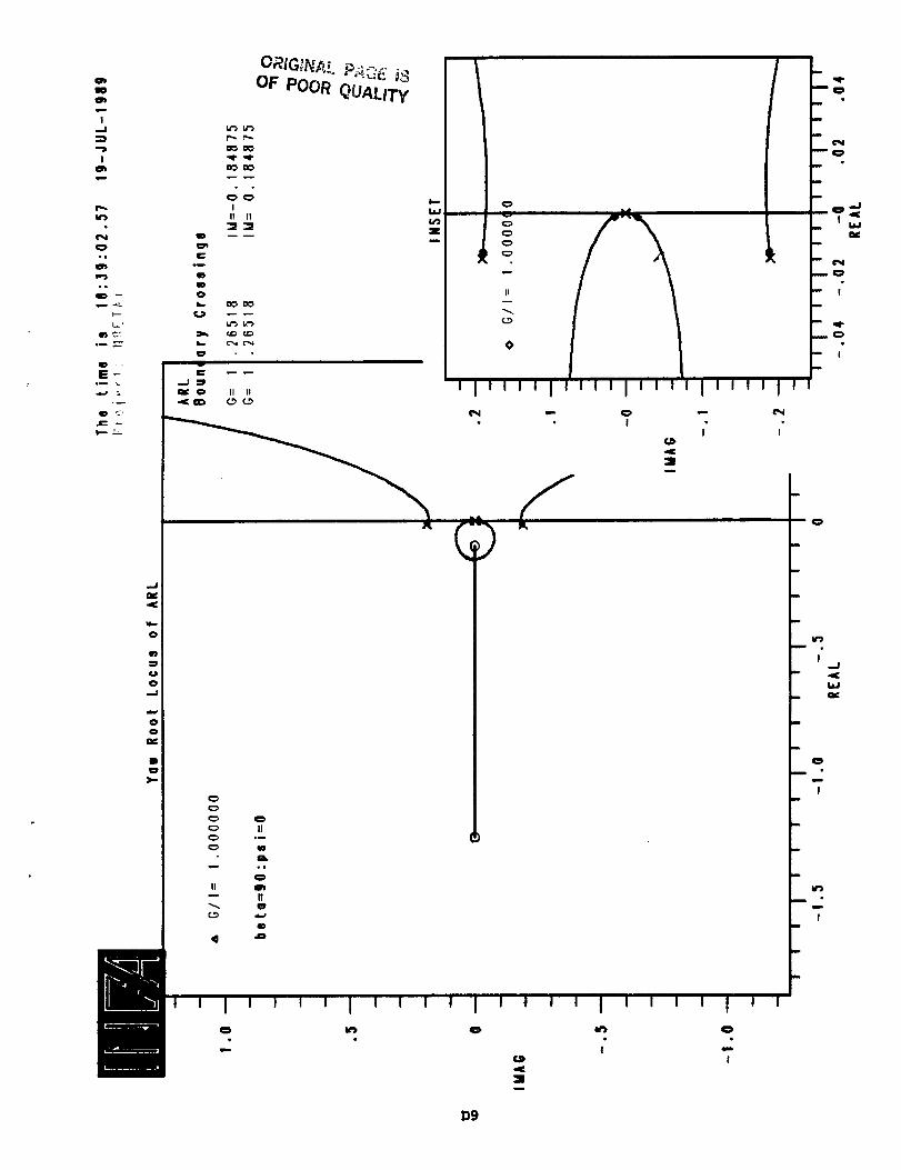
D9 13_90 control law yaw loop 90 45

D10 13_=90 control law yaw loop 45 0

D1

0 !

II

I

!

1

D2

IO

m

i

i

Z

,,,¢

!

c'_

¢h

p,.,=

t,D

m

L=-'

,i --

I=--,i ...-

¢D,,.

O

O

_.I

D

:=,-.

O

qD

u

..,.]

=,=i

O_GINAL PAGE t_

OF _R QUALITY

=..°_

IrJ

O

r'.-

=OClO

w

c_,_

!

!I il

"J= :_I

"_ ',,,e-

t_ C_

S*")

Z

.,I= 0 tl f;

c_

c_

C_

It

,,,i,,,/¢_f m I0

I

I

-a=

¢"W

I

I

,.J

n..,

C_

C",,,l

¢=,

-.J

t'N

I

|. •

I I

D3

I

=i iin ill |1 --

,.,'J" OF POOR QUALITY

_ -r5 -°

_._. =_, __l_ Jl _- _ ............ "

2

O

o

I

!

I

O'J

m

I

Z

I

,,q,.

n-,

'ID -

jr" _

OR,_o,,_,._ P:],GE IS

OF POOR QUALITY

i I I I

II

¢

I

I

I

I

I I

m_

m

m

I

I

m• '_I i. _

D_

m

I

D5

!

!

ql"

m_

_r'> it> I--, _ Q .

• " _1 _ _ I'1_I _ I

_--- 0 L,h,,I I,_ | _

l

, .-.,- Lt : , , i : i i a i_2 _ ,_,_ : , I ! 11 i I t i I t I I ! ' '

0 II 11 - I • "

,L,,_,,__ _ _ ! I

_3

- -o P_GE IS=__ OFPOOR UA _"

'r l"UOR QUALITY I-

i t T--

m

w

m

m

!m

m

I

I

D6

II

I

D7

I

ORiG_,'_h,= PAGEOF POOR QUALITY

{".W

'lO I I

I_. _.a.J [aJ

I ,.o r.o

=_ f..l=, f._

I e.... r.--

Ir'w

I

II II

elm

o--

** IlID

O

.=

o-- _.I=

E- ,,.,o

I I

LLJ l.i.l

•q- 'ql"

•q=,-_

It It

___ _._

I,--

z

m

m

11

4

lll lltllllStJllJllll I

I

3

I"

I

D8

m

io

T

.--j

I

¢h

r_

c_.i

m

..

L,._,

qD --

IE--

qD _"

O'_DO

I

11 II

9D

qlO

0

II_ rJ_ rj_

.==/

0 II II

OF POOR QUALITy

I'--

ELI

V'J

Z

m

IIm

O

Jllllll I I

0

I

0

O

..1

-g0

B

]p-

¢_

C_

C_, O

c_, U

c_

O

II m

N

4D

4 "_

¢,D

m

J I I

I"

I I J !

I"

m

n

m

m

m

m

m

.,,J

! W

O1[m

m

n

_O

-- I

J

0

m

m

I..I

la, J

m

!m

m

m

Im

D9

!

!

w-

,o

=J

L

0

...J

0

D

iwu

_ v

°

II

I°

I_I II'I_I I ! I I I I I

°

f:

_) -

ORIGINAL PAGE °_J3

OF POOR QUALITY

I I I

m

m

m

w

I

ms

m

Im

w

m

m

m

!m

m

m

o •

! l

!

DIO

¢1=

lib

w

!

!

tlD

°,

,i

t=Lf

m• w _._

Q -.

t=-

I,-. F...-

c

o_

II

¢=0

0

0

ml=

m

D11

Appendix E

Simulation Plots

The following pages contain plots of the performance of the IUE

satellite in response to various slew maneuvers using the zero-gyro

control laws as predicted by the low-fidelity simulation. The plots

represent the movement of the satellite in terms of its three

rotation angles, alpha, beta, and psi. In some cases, the rate of

rotation about the sunline is examined instead of the psi angle (this

is labelled psi rate) due to the difficulty in computing the actual

angle psi within the simulation itself. The plots represent the

following control laws and commanded angles:

E1

E2

E3

E4

E5

E6

E7

E8

E9

El0

,8 (deg)

13=90 linear control law 91 0

13=90 linear control law 90 44

13=90 non-linear control law 90 5

_=90 non-linear control law 90 44

13_90 linear control law 91 0

13_90 linear control law 90 44

_90 linear control law 45 0

13_90 non-linear control law 91 0

_90 non-linear control law 90 44

_90 non-linear control law 45 0

(deg)

E1

rife: rUEEA JUT the lime Is 14:35:4_,Sl 26-F_B-_lB!

BETA-If:PSI=O,0;_OHIHAL ;AIM$;TSAWP-O,2AL_HA

.I0

.05

i -°O5

10

!1 .5

gl .010 5

IO .0

5i°-5

-10

! 1 I ! I I I

E2

_ir_: IUEEA gUT

BETkolO;PSla=44;HOHIH_L G_INS ¢2_LpH _

The time is 1i:18:5B.07 21-F[B-IISI

01 -"

-D

-.01

- g2w ,, . .. , i

, , i , I ' ' ' ' I ' ' w , I1000 2000 _ _,gOO

i

4QO_ 5_

gO 01

81 l!

4000

10

4_00

5O

E3

UD

O

m-

I

.ml

I

.o

ID

J

o

J_

i-..

o

m

_D

m

g

¢)

c

.o

Q

t_

B_m

E0

II

-- ¢)

m

• " If

W

I--/1 I t I i I I

m

m

m

m

m_

m

m

m

m

m

m

m

w_

_m

m

m

_0

w

w

0

0 0 0 m m

¢_ 0 0 4_ m

4_ _ 818 DO

E4

!

--J

==)

I

w'#

w')

t_

o.

qrJ

°_

Eol

..1=

I-.-

I=1

,C

qD

D

!

t=

O

I=

16

,w

C

EO

I=

I1

._- ,m

_ZF ,a

"" II

w

,m 0

L_- ,a

.... '.... J- , C:_

U")

_._C

r_ " " " _ U_' .

t'q

t_

r'q

° ___ ° °

....

0 0 0 _'

O q" I_I0 0 0 _h

0 _ _ gtI I

Ill

Dm

!

!

tin)*o

w

l

m

Q.

Q..

Zm

.J

Z

,.J-CZ

O

•7 e

"" I!

i I--

t'_ 0 t'_ ql"! Q Q

I0 C:)

u_umm

glIO

I,--,I

I

P,,l..P,,l

o.

w

II

II

E.m

o

I..--

01:

Zm

.--I

+.

X

'51ID

i-- ++

- II

l+._ O,.

-- ,_

o',i.- If

--

.-- i_i

t..,._

Z

o,,.,,.J

LIJQD

Q.

i n

< <)> °

> "+

i

Q

i m

),+. ( o

r

c",,lO

I" I _' O

'llJllleil0' o,, o,+mBo

Ol

010

O O Q

olw, r.J3_ilO

E7

0wl.

I

I"ql"

O

-4.

im

Io

r'.

mq_

DE

ZCb..J

laJ

m

0.

Zm

Zw.m

II

,0

• - I!

.-- Ld

1" O

O...... O

O

•.-,.ram U

q_' ql* .qm ql" ° * °

F_ Im

E8

Q

O

qm

mD

lira

4m,

!

iJ

!

c_J

o

o

w-J

Q

ol

wl

w

Q

E4_

Q

P

Z

r_

°_

.o

V_

Z

--J

14C

LAJ

_E

II

!

Z

0

Z

oo

Z

4_

_J

-.IFm

,!O

Z

_a

I!

u

Q,

gw

CB_

l!

W,m

nr_

O 10

m m

f

C_

Jl

c_

m

_mUllb.L

_1 _m m 0 O

jma

q_ r_l Q C_

I

ummta

E9

I8O

sin,I

--I

I

v7

.°

v_

.°

m

w

QE

.u

Q

I,--

Z¢1..,,,J

Z

--J!

Z0Z,6

.j,m

Z

1o

II

0_j--_, ,j

-- 14")qr

"-- WtL. ¢D

_r

EIO

i

0

I

O

!m_

!

Ell

Report Documentation PageNalolal Aefon_licsand_c_._*eACIrnl+_slralo+,

1. Report No.

NASA TM-I00748

4. Title and Subtitle

2. Government Accession No. 3. Recipient's Catalog No.

5. Report Date

Analytical Derivation and Verification of Zero-Gyro

Control for the IUE Satellite

7. Author(s)

Tiffany Bowles and John Croft

9. PedormingOrganizationNameand Address

Goddard Space Flight Center

Greenbelt, Maryland 20771

12. Sponsoring AgencyNameand Addre_

National Aeronautics and Space Administration

Washington, D.C. 20546-0001

November 1989

6. Performing Organization Code

712

8. Pedorming Organization Report No.

89B00245

10. Work Unit No.

11. Contract or Grant No.

13. Type of Report and Period Covered

Technical Memorandum

14. Sponsoring Agency Code

15. Supplementary Notes

16, Abstmct The International Ultraviolet Explorer (IUE) satellite was launched

January 26, 1978 into a geosynchronous orbit over South America. From its

stationary position, the telescope maintains continuous communication with

the control centers at NASA's Goddard Space Flight Center in Greenbelt, Mary-

land, and at the European Space Agency's (ESA's) Villafranca del Castillo

Satellite Tracking Station in Spain. Since its launch in 1978, the satellite

has gradually lost four of the original six gyroscopes in the Inertial Reference

Assembly (IRA). In August 1985, the fourth of the original six gyros failed and

a two-gyro system developed by NASA-GSFC was uplinked to the satellite and is

currently in use. A one-gyro system also developed by NASA-GSFC is ready for

use in case of another gyro failure. In the event that the sixth gyro should

also fail, a zero-gyro system is being developed. The goal of this system is to

provide inertial target pointing without the use of gyroscopes. The satellite

has sun sensors to provide attitude information about two of the three axes.

It relies upon the exchange of reaction wheel momenta to determine angular

position and rate of the third axis.

17. Kw Words(Suggem_ byAuthor(s))

International Ultraviolet Explorer,

attitude gyros, satellite guidance,

inertial reference systems

19. Security Classif. (of this report)

Unclassified

NASA FORM 1626 OCT 86

18. Distribution Statement

Unclassified - Unlimited

Subject Category 18

20. Security Cla_if.(ofthispage)

Unclassified

21 No. of pages

45

22. Price