analytical and numerical solutions of ...im.pcz.pl/konferencja/dokumenty/mmft2017/ciesielski...
TRANSCRIPT

ANALYTICAL AND NUMERICAL SOLUTIONS
OF DIFFERENT TYPES OF EQUATIONS
USED FOR MODELING HEAT CONDUCTION
UNDER LASER PULSE HEATING
Mariusz CiesielskiInstitute of Computer and Information Sciences,
Czestochowa University of Technology, Czestochowa, Poland
IX Konferencja Modelowanie Matematyczne w Fizyce i Technice (MMFT 2017) 18-21.09.2017, Poraj

Introduction
In the paper, the problem of heat transfer proceeding in a thin film subjected to a short pulse laser heating is considered.The mathematical model presented concerns a 1D problem.For most short laser pulse interactions with thin films, the laser spot size is much larger than the film thickness.
Domain considered
The pulse duration is of the order of femtoseconds (1 fs = 10"#$ s).The thickness of the film is of the order of nanometers& ~ 100 − 200 nm (1 nm = 10"* m)

Introduction
Experimental dataS.D. Brorson, J.G. Fujimoto, E.P. Ippen, Femtosecond electronic heat-transport dynamics in thin gold films, Phys. Rev. Lett. 59, 1987, pp. 1962-1965.T.Q. Qiu, et al., Femtosecond laser heating of multi-layer metals - II. Experiments, International Journal of Heat and Mass Transfer 37, 17, 1994, pp. 2799–2808.
Schematic of the experimental setup Front-surface data for Au films Auto-correlationof laser pulses
1 Å = 0.1 nm
Introduction
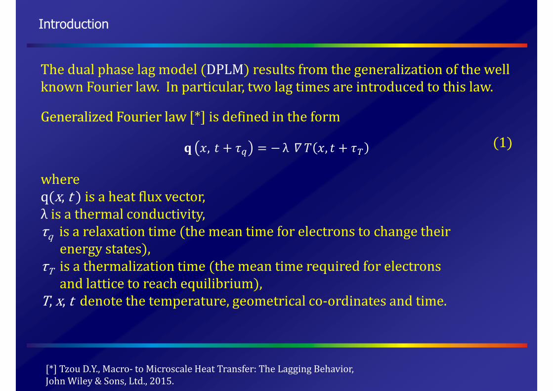
The dual phase lag model (DPLM) results from the generalization of the well known Fourier law. In particular, two lag times are introduced to this law.Generalized Fourier law [*] is defined in the form (1)where q(x, t ) is a heat flux vector, λ is a thermal conductivity, τq is a relaxation time (the mean time for electrons to change theirenergy states), τT is a thermalization time (the mean time required for electrons and lattice to reach equilibrium), T, x, t denote the temperature, geometrical co-ordinates and time.
J L, M + OP = − λ Q R L, M + OS
[*] Tzou D.Y., Macro- to Microscale Heat Transfer: The Lagging Behavior, John Wiley & Sons, Ltd., 2015.

Introduction
Using the Taylor series expansions, the following first-order approximation of Eq. (1) can be taken into account
Next, this formula is introduced to the well known macroscopic energy equation
wherec is a volumetric specific heat, Q is a capacity of internal heat sources.
J L, M + τP ZJ L, MZM = − λ QR L, M + τS Z QR L, MZM
[ ZR L, MZM = −Q ⋅ J L, M + ^ L, M

Introduction
Finally, the energy equation called the dual phase lag equation is defined as(2)
In 1-D Cartesian coordinates and for `=const :If OP = 0, OS = 0 : the Fourier-type heat conductionIf OP > 0, OS = 0 : the hyperbolic Cattaneo-Vernotte modelIf OP > 0, OS > 0 : the DPLMThe energy equation is the hyperbolic PDE containing a first and second order time derivative and higher order mixed derivative in both time and space. Dual phase lag equation is supplemented by the appropriate boundary and initial conditions.
[ ZR L, MZM + OP ZcR L, MZMc = Q ⋅ λ QR L, M + OS Z Q ⋅ λ QR L, M ZM+ ^ L, M + OP Z^ L, MZM
Q ⋅ λ QR L, M = λ Zc R L, MZ Lc

Introduction
Initial-boundary conditionsThe Eq. (2) is supplemented by the no-flux conditions(3)where d ⋅ Q R L, M is a normal derivative.One can see, that the Neumann-type boundary condition differs from the similar one in the classical heat conduction model.
The initial conditions for the problem considered are of the form(4)where T0(x) is the known temperature and T1(x) is the initial heating rate (for the task considered T1(x) is assumed to be equal to 0).
L ∈ g: − ` d ⋅ QR L, M + OS Z d ⋅ QR L, M Z M = 0
M = 0: R(L, M) = Rh(L), Z R(L, M)Z M |jkh = R#(L)

Introduction
The effects of the femtosecond laser pulse irradiation on the surface x = 0 causes that the energy is delivered into the metal and its absorption occurs. The internal heat source Q (x, t) generated inside of metal is related with the action of laser beam
where I0 is a laser intensity, R is a reflectivity of irradiated surface, δ is an optical penetration depth, β = 4 ln2,tp is a characteristic time of laser pulse.
^ L, M = lm 1 − nMop qhexp − Lp − l M − 2MoMoc

Analitytical solution
The solution of the 1D hypergeometric PDE (2) with the initial conditions (4) and the no-flux boundary conditions (3) can be found in the general form as [*]
where r L, s, M is the Green functionand t L, M = #u vw ^ L, M + OP xy z,jxj .
R L, M = { { t s, O r L, s, M − O|h
}s}Ojh
− { Rh s|h
ZZO r L, s, M − O vkh }s + { R# s + 1OP Rh s r L, s, M }s|h
[*] Polyanin A.D., Nazaikinskii V.E., Handbook of Linear Partial Differential Equations forEngineers and Scientists, Second Edition, CRC Press, Boca Raton-London, 2016.

Analitytical solution
The Green function r L, s, M is determined by solving the following homogenous equation
which satisfies the initial conditionsand the homogenous boundary conditionsThe Green’s function can be expressed as
where functions �� and �� should be determined. [*] Polyanin A.D., Nazaikinskii V.E., Handbook of Linear Partial Differential Equations forEngineers and Scientists, Second Edition, CRC Press, Boca Raton-London, 2016.
r L, s, M = � �� L �� s‖��‖ �� M�
�kh, ‖��‖ = { ��c L|
h }L
Zr L, s, MZL |zkh = 0, Zr L, s, MZL |zk| = 0r L, s, M |jkh = 0, Zr L, s, MZM |jkh = p L − s
Zcr L, s, MZMc + 1OPZr L, s, MZM = `[OP Zcr L, s, MZLc + OS Z�r L, s, MZMZLc

Analitytical solution
The particular solution of Eq. (2) for t L, M = 0 is the product of the functions (*)Introducing Eq. (*) into Eq. (2) (and omitting the term t L, M )one obtains the equation
Separating variables, we obtain
where the two expressions have been set equal to the constant −��c .
R L, M = � L � M
[ � L d � Md M + OP� L d c� Md Mc = ` d c� Ld Lc � M + OS d c� Ld Lc d � Md M
[̀ OP d c� Md Mc + d � Md M� M + OS d � Md M = d c� Ld Lc� L = −��c

Analitytical solution
This yields two ODE’s: (*)(**)The eigenfunctions and eigenvalues of the Sturm-Liouville problem (*) with the
boundary conditions d� zdz |zkh = 0, d� zdz |zk| = 0are the followingThe functions �� are determined by solving Eq. (**) with the initial conditions � 0 = 0 and d� M d⁄ M|jkh = 1 . For OP < OS the solution of the considered initial problem simplifies to the form
where
d c� LdLc + ��c� L = 0,
OP d c� Md Mc + 1 + ��c [̀� OS d� MdM + ��c [̀� � M = 0
�� L = cos ��L , �� = �m& , � = 0,1, . . .
�� M = exp −}� M sinh �� M�� }� = 12OP 1 + ��c [̀ OS �� = }�c − ��c [̀ 1OP

Analitytical solution
The analytical solution of the initial-boundary value problem (2)-(4) under the assumption that OP < OS is the following [*](5)where
R L, M = t �h M + 2 � cos ��L �� M��k# + Rh
t = 1 − n qh[OP&
�� M = 1 − −1 �exp − & p⁄1 + pc �� c exp −4l4�� �2 lm OPMo exp − }� + �� M − exp − }� − �� M+ 1 − OP }� + �� exp ��� c − }� + �� M erfc ��� − erfc ��� − lMo M− 1 − OP }� − �� exp ��" c − }� − �� M erfc ��" − erfc ��" − lMo M �
�� = �m& }� = 12OP 1 + ��c [̀ OS �� = }�c − ��c [̀ 1OP��± = 2 l + j�c � }� ± �� n = 0,1,….[*] M. Ciesielski, Analytical solution of the dual phase lag equation decribing the laser heating of thin metal film, Journal of Applied Mathematics and Computational Mechanics, 2017, 16, 1, 33-40.

Numerical solution
To find the approximate solution of the problem (2)-(4) the Control Volume Method (CVM) is used.The first stage of the method application is the division of the domain considered into N +1 small cells (known as the control volumes CV) with the central nodes 0 = x0 < x1 < … < xi < … < xN = L , xi = i ∆x , ∆x = L/N .The values of the successive volumes ∆Vi and the values of surfaces ∆Ailimiting CV can be easily determined.
Mesh of control volumesThe aim of the CVM is to find the transient temperature field at the set of control volumes.

Numerical solution
The average temperatures in the all control volumes can be found on the basis of energy balances for the successive CV. The energy balances corresponding to the heat exchange between the analyzed control volume and adjacent ones result from the integration of energy equation with respect to volume and time.Integration of Eq. (2) over the control volume CVi leads to
(6)[ � Z R L, MZ M + OP Zc R L, MZ Mc }����
= ` � Zc R L, MZ Lc + OS ZZ M Zc R L, MZ Lc }����
+ � ^ L, M + OP Z^ L, MZ M }����

Numerical solution
The integral occurring on the left-hand side of Eq. (6) can be approximated in the form (7)where R� ≡ R(L� , M). In a similar way the numerical approximation of the source term in Eq. (6) can be found (8)where ^� ≡ ^� M is the average value of the heat source in the volume CVi .• ^� ≅ ^ L�, M - the simplest way, but inexact approximation,• ^� ≅ #¢�� £ ^ L, M }���� - can be calculated analytically or using numerical integration methods.
[ � Z R L, MZ M + OP Zc R L, MZ Mc }����
≅ [ d R�d M + OP d cR�d Mc ¤¥�
� ^ L, M + OP Z^ L, MZ M }����
≅ ^� + OP d ^�d M ¤¥�

Numerical solution
Applying the divergence theorem to the term determining heat conduction (right hand side of Eq. (6)) between the volume CVi bounded by the surfaces ∆Ai and its neighbourhoods one obtains (taking into account the boundary conditions)
(9)wherewhile n = ¤ L `⁄ is the thermal resistance.
` � Zc R L, MZ Lc + OS ZZ M Zc R L, MZ Lc }����
= ` d ⋅ � ZR L, MZ L + OS ZZ M ZR L, MZ L }§¨�
≅ ` ¤§�
R# − Rh¤L + OS }}M R# − Rh¤L for � = 0R��# − R�¤L + OS }}M R��# − R�¤L + R�"# − R�¤L + OS }}M R�"# − R�¤L for � = 1, . . . , © − 1Rª"# − Rª¤L + OS }}M Rª"# − Rª¤L for � = ©
= ¤§� «�«� = R��# − R�n + OS }}M R��# − R�n ¬® �¯ª + R�"# − R�n + OS }}M R�"# − R�n ¬® �°h

Numerical solution
Putting Eqs. (7)-(9) into Eq. (6), one obtains
or (10)where
[ d R�d M + OP d cR�d Mc ¤¥� = «� ¤§� + ^� + OP d ^�d M ¤¥�
[ d R�d M + OP d cR�d Mc = «� t� + ^� + OP d ^�d M
t� = 1¤L , for � = 1, . . . , © − 1, th = tª = 2¤L

Numerical solution
The second stage of CVM is the integration of Eq. (10) with respect to time. So, the time grid: 0 = t 0 < t 1 < … < t f < … < t F, t f = f ∆t is introduced.The Crank-Nicolson method involves a combination of implicit and explicit schemes. The energy balance for the transition M± → M±�#, f = 2,...,F written in the convention of the α-scheme takes the form
(11)
where α ∈ [0,1] is the weighting factor (α = 0 leads to the ‘explicit’ scheme, and α = 1 to the fully ‘implicit’ scheme).
[ R�±�# − R�±¤M + OP R�±�# − 2R�± + R�±"#¤M c
= ´ «�±�#t� + 1 − ´ «�±t� + ^�±�# + OP ^�±�# − ^�±¤M

Numerical solution
After the transformations, the following system of equations is obtained(12)
where �P = OP ¤⁄ M, �S = OS ¤⁄ M and
From the initial conditions (4) results R�h = R�# = Rh.µ�"#± = ´�S − 1 − ´ 1 + �Sn R�± − R�"#± + 1 − ´ �Sn R�±"# − R�"#±"#µ��#± = ´�S − 1 − ´ 1 + �Sn R�± − R��#± + 1 − ´ �Sn R�±"# − R��#±"#
[ 1 + �P¤M + ´ 1 + �Sn t�¶® � ¯ª + ´ 1 + �Sn t�¶® �°h R�±�# − ´ 1 + �Sn t�R��#±�#¶® �¯ª− ´ 1 + �Sn t�R�"#±�#¶® �°h
= [ 1 + 2�P R�± − �PR�±"#¤M + µ�"#± ·® �°h + µ��#± ·® �¯ª t� + 1 + �P ^�±�# − �P^�±
for � = 0, . . . , ©

Example of computations
The 1D domain (plate) with dimensions L = 100·10-9 m is considered.Thermophysical parameters of thin film (gold): λ = 317 W/(mK), c = 2.4897·106 J/(m3K), τq = 8.5·10-12 s, τT = 90·10-12 s.The parameters of the laser pulse: I0 = 13.7 W/m2, R = 0.93, δ = 15.3·10-9 m, tp = 100·10-15 s. The initial temperature of the metal: T0 = 20 oC.

Results of computations
The analytical solution of the DPL equation
The temperature histories at the selected points from the domain:x = {0, 25, 50, 100 nm}The temperature profilesfor the times:t = {0.2, 0.5, 1, 3 ps}

Results of computations
The numerical calculations wereperformed for different time meshsizes: ∆t = {10-15, 10-16, 10-17 s}and ∆x = 10-9 m (N = 100)α = 0.5
The errors of the numerical solutions (the Crank-Nicolson method)¤R L, M = R¼�¼½¾j�u¼½ L, M − R�¿ÀÁÂ�u¼½ L, M

Results of computations
The numerical calculations wereperformed for different time meshsizes: ∆t = {10-15, 10-16, 10-17 s}and ∆x = 10-10 m (N = 1000)α = 0.5
The errors of the numerical solutions (the Crank-Nicolson method)¤R L, M = R¼�¼½¾j�u¼½ L, M − R�¿ÀÁÂ�u¼½ L, M

Results of computations
The numerical calculations wereperformed for ∆t = 10-16 s, ∆x = 10-9 mat the points x = (0, 25, 50 nm).In Figures, the influence of parameterα ={0, 0.5, 1} on numerical errors ispresented.
The errors of the numerical solutions (the Crank-Nicolson method)¤R L, M = R¼�¼½¾j�u¼½ L, M − R�¿ÀÁÂ�u¼½ L, M

Results of computations
The influence of different values of parameters τq , τT on the solutionsDPLM
τq = 8.5·10-12 s, τT = 90·10-12 s.
C-V modelτq = 8.5·10-12 s,
τT = 0 s.
Fourier modelτq = 0 s, τT = 0 s.

Conclusions
Heat transfer processes can be described using the Fourier and non-Fourier heat conduction models, but the dual phase lag model seems to be adequate for mathematical description of microscale heat transfer. One of the main subjects of the paper is the comparison of the results obtained using the analytical and numerical methods. In the case of the numerical solution, the control volume method and Crank-Nicolson schemehave been used.The results of numerical computations confirm the effectiveness of the presented algorithm.The 1D solution of the problem discussed is, as a rule, sufficiently exact, but the author has developed the computer programs realizing the computations for geometrically more complex domains.