C

Ao

YDa

b

c

h

•

•

•

a

ARR1AA

KVIPIR

1

bhi

f

0h

Analytica Chimica Acta 807 (2014) 36– 43

Contents lists available at ScienceDirect

Analytica Chimica Acta

jou rn al h om epage: www.elsev ier .com/ locate /aca

hemometrics

strategy that iteratively retains informative variables for selectingptimal variable subset in multivariate calibration

ong-Huan Yuna, Wei-Ting Wanga, Min-Li Tana, Yi-Zeng Lianga,∗, Hong-Dong Lia,ong-Sheng Caob, Hong-Mei Lua, Qing-Song Xuc

College of Chemistry and Chemical Engineering, Central South University, Changsha 410083, PR ChinaCollege of Pharmaceutical Sciences, Central South University, Changsha 410083, PR ChinaSchool of Mathematics and Statistics, Central South University, Changsha 410083, PR China

i g h l i g h t s

Considers the possible interactioneffect among variables through ran-dom combinations.Four kinds of variables were distin-guished.It was more efficient when comparedwith CARS, GA-PLS and MC-UVE-PLS.

g r a p h i c a l a b s t r a c t

r t i c l e i n f o

rticle history:eceived 21 August 2013eceived in revised form3 November 2013ccepted 14 November 2013vailable online 21 November 2013

a b s t r a c t

Nowadays, with a high dimensionality of dataset, it faces a great challenge in the creation of effectivemethods which can select an optimal variables subset. In this study, a strategy that considers the possibleinteraction effect among variables through random combinations was proposed, called iteratively retain-ing informative variables (IRIV). Moreover, the variables are classified into four categories as stronglyinformative, weakly informative, uninformative and interfering variables. On this basis, IRIV retains boththe strongly and weakly informative variables in every iterative round until no uninformative and inter-

eywords:ariable selection

nformative variablesartial least squaresteratively retaining informative variables

fering variables exist. Three datasets were employed to investigate the performance of IRIV coupled withpartial least squares (PLS). The results show that IRIV is a good alternative for variable selection strategywhen compared with three outstanding and frequently used variable selection methods such as geneticalgorithm-PLS, Monte Carlo uninformative variable elimination by PLS (MC-UVE-PLS) and competitiveadaptive reweighted sampling (CARS). The MATLAB source code of IRIV can be freely downloaded for

webs

andom combination academy research at the

. Introduction

Variable (feature or wavelength) selection techniques have

ecome a critical step in the analysis for the datasets withundreds of thousands of variables in several areas. These areas

nclude genomics, bioinformatics, metabonomics, near infrared

∗ Corresponding author. Tel.: +86 731 8830824/+86 13808416334;ax: +86 731 8830831.

E-mail addresses: yizeng liang@263.net, yizengliang@gmail.com (Y.-Z. Liang).

003-2670/$ – see front matter © 2013 Elsevier B.V. All rights reserved.ttp://dx.doi.org/10.1016/j.aca.2013.11.032

ite: http://code.google.com/p/multivariate-calibration/downloads/list.© 2013 Elsevier B.V. All rights reserved.

and Raman spectroscopy, and quantitative structure-activity rela-tionship (QSAR). The goal of variable selection can be summarizedin three aspects: (1) improving the prediction performance of thepredictors, (2) providing faster and more cost-effective predictorsby reducing the curse of dimensionality, (3) providing a betterunderstanding and interpretation of the underlying process thatgenerated the data [1,2]. In the face of the situation that the num-

ber of samples is much smaller than the number of variables (largep, small n) [3,4], a large amount of variable selection methods hasbeen employed to tackle this challenge in the field of multivari-ate calibration. There are two directions in these methods. One is

Chimi

bcmk[r(eaoogss(cpbahicabpobBfatrdDsBh

nmiuibtvogHatiacitIeaiivt

ws

Y.-H. Yun et al. / Analytica

ased on statistical features of the variables through some kind ofriteria, such as correlation coefficient, t-statistics and Akaike infor-ation criterion (AIC), and selects the significant variables. This

ind of method includes uninformative variable elimination (UVE)5], Monte Carlo based UVE (MC-UVE) [6], competitive adaptiveeweighted sampling (CARS) [7,8], successive projection algorithmSPA) [9], random frog [10,11]. Although they have computationalfficiency, a common disadvantage is that they select the vari-bles individually while ignoring the joint effect of variables. Thether kind is based on the optimized algorithm to search theptimal variables. However, since the space of variable subsetsrows exponentially with the number of variables, a partial searchcheme is often used, such as stepwise selection [12], forwardelection [12,13], backward elimination [12–14], genetic algorithmGA) [15–21] and simulated annealing (SA) [22]. It is unpractical toonduct the greedy search by exhaustively searching through allossible combinations of variable sets. The process of finding theest variable subsets, not only using an effective search scheme butlso considering the interaction of variables in the search space,as been an important part in variable selection research. Margin

nfluence analysis (MIA) proposed by Li et al. [23] considers theombination of variables using Monte Carlo sampling techniquend ranks all the variables based on P value of hypothesis testing,ut the number of variables to be sampled is often set to be a fixedarameter predefined by user’s input. Sampling a fixed set numberf variables result in the chance of every variable to be sampled noteing the same. Some are selected more frequently, but some not.inary matrix shuffling filter (BMSF) [24] provides effective search

or informative variables in the infinite dimensional search space,nd also considers the synergetic effect among multiple variableshrough random combination. It consists of a guided data-drivenandom search algorithm using a binary matrix to convert the high-imensional variables space search into an optimization problem.ifferent from MIA, BMSF assures that all the variables have the

ame chances to be sampled with the binary matrix. Furthermore,MSF is an iterative filtering algorithm [25] which eliminate aboutalf of the variables on each round of filtering using a criterion.

Based on the core idea of BMSF, in this study, we propose aovel variable selection strategy, called Iteratively Retaining Infor-ative Variables (IRIV). Additionally, we also divided the variables

nto four categories as strongly informative, weakly informative,ninformative and interfering variables, which is regarded as an

mprovement of the definition on the classification of variablesy Wang and Li [26], where the variables are only classified intohree categories, as informative, uninformative and interferingariables. Their definition is illustrated in next section. As the namef IRIV implies, it conducts many rounds until it reaches conver-ence. For every round, a large amount of models is generated.ere, we introduce a novel methodology called model populationnalysis (MPA) [23,26–28] to distinguish the four kinds of variableshrough the analysis of a ‘population’ of models. Generally, stronglynformative variables indicate that they are always necessary forn optimal subset. Some variable selection methods use them toonstitute the optimal variable set ignoring the effect of weaklynformative variables. However, weakly informative variables con-ribute as well due to their beneficial effect. Based on this idea,RIV retains both the strongly and weakly informative variables invery iterative round until no uninformative and interfering vari-bles exist. When compared to obtaining the informative variablesn one round, this approach can avoid that some uninformative andnterfering variables appear in the strongly and weakly informativeariables set by chance. Finally, backward elimination is conducted

o obtain the most optimal variable set.

In this work, IRIV coupled with partial least squares (PLS) [29]as investigated through the analysis of three real near infrared

pectral datasets and better results were obtained than with the

ca Acta 807 (2014) 36– 43 37

three outstanding methods. This demonstrates that IRIV is a goodalternative of variable selection algorithm for multivariate calibra-tion. It should be pointed out that although IRIV was just testedby NIR dataset, it is a general strategy and can be coupled withother regression and classification methods and applied for otherkinds of data, such as genomics, bioinformatics, metabonomics andquantitative structure–activity relationship (QSAR) [30].

2. Methods

Given that the data matrix X contains N samples in rows andP variables in columns, and y, of size N × 1, denotes the measuredproperty of interest. In this study, PLS was used as multivariatecalibration method in the IRIV strategy. The detailed approach ofIRIV is illustrated as follows:

Step 1: In order to consider the combination of multiple vari-ables to be used for modeling, a binary matrix M that just containseither 1 or 0 with dimensions K × P is generated. K is the number ofrandom combination of variables. P is the number of variables. Thenumber “1” represents the variables that are included for modeling,while 0 represents the variables that are not included. It should bementioned that the binary matrix M contains KP/2 ones and KP/2zeros, which guarantees that there are the same choices for all vari-ables to be included or excluded for modeling. Besides, the M ispermuted by column. The number of ones and zeros in each col-umn is the same. Each row of M determines which variables are tobe considered for modeling. Different rows of M give different vari-ables sets that contain different combinations of a random numberof variables. This process is clearly illustrated in Fig. 1A.

Step 2: Each row of M is used for modeling with PLS method.Here, the mean squared error of five-fold cross validation (RMSECV)is used to assess the performance of each variables subset. Thus, aRMSECV vector (K × 1), denoted as RMSECV0, can be obtained.

Step 3: For the sake of assessing each variable’s importancethrough its interaction with other variables, a novel strategy isused. That is, in a variable set (a row of M), the performance ofthe inclusion and exclusion of one variable is compared, while thestate (inclusion or exclusion) of other variables are left unchanged.Thus, for the ith (i = 1, 2, . . ., P) variable, we can obtain matrix M1by changing all the ones in ith column of M to zero and all the zerosin ith column to one, while keeping other columns of M unchanged(shown in Fig. 1B). RMSECVi (K × 1) can be obtained after finish-ing all rows of Mi. Then, ˚0 and ˚i are collected to assess theimportance of each variable as the following formulas:

˚0k ={

kthRMSECV0 if Mki = 1

kthRMSECVi if M1ki = 1, ˚ik =

{kthRMSECV0 if Mki = 0

kthRMSECVi if M1ki = 0(1)

Where Mki is the value in the kth row and ith column of M, andM1ki is the value in the kth row and ith column of M1. Briefly, ˚0collects the value of RMSECV0 and RMSECVi that the ith variable isincluded in the variable set for modeling, while ˚i collects the valueof RMSECV0 and RMSECVi that the ith variable is excluded in thevariable set for modeling. Notice that the values of ˚0 and ˚i areput in the same order as the rows of M. Such arrangement ensuresthat the ˚0 and ˚i are in pairs so as to focus on how significantthe ith variable makes a contribution with various combinationsof multiple variables in the modeling, while the conditions of theother variables are held the same. Both ˚0 and ˚i contain theresults of K models. Therefore, model population analysis (MPA)[23,26–28,31] can be used to analyze the variable importance withthese two ‘population’ models.

Step 4: Calculate the average value of ˚ and ˚ , denoted as

0 iMEANi,include, MEANi,exclude. The difference of the two mean valuescan be calculated as:

DMEANi = MEANi,include − MEANi,exclude (2)

38 Y.-H. Yun et al. / Analytica Chimica Acta 807 (2014) 36– 43

orman

wdnPwsdwi

V

V

V

V

wVuanamTDbs

ran

aeitmf

(

(

Fig. 1. (A) the process of generating binary matrix; (B) the perf

Here, the four kinds of variables, such as strongly informative,eakly informative, uninformative and interfering variables, can beistinguished by Eq. (2) and hypothesis testing. In this study, theonparametric test method, the Mann–Whitney U test [32], is used.

value, denoted as Pi, is computed by the Mann–Whitney U testith the distribution of ˚0 and ˚i. With respect to statistics, the

maller Pi value, the more significant difference between the twoistributions. P = 0.05 is predefined as the threshold. In this sense,ith the P value and DMEANi, we can easily classify the variables

nto four categories as follows:

i ∈ Vstrongly informative if DMEANi < 0, Pi < 0.05 (3)

i ∈ Vweakly informative if DMEANi < 0, Pi > 0.05 (4)

i ∈ Vuninformative if DMEANi > 0, Pi > 0.05 (5)

i ∈ Vinterfering if DMEANi > 0, Pi < 0.05 (6)

here Vstrongly informative, Vweakly informative, Vuninformative andinterfering indicate that strongly informative, weakly informative,ninformative and interfering variables, respectively. From thebove definition, we can see that the strongly informative variablesot only have a beneficial effect on the modeling (DMEANi < 0), butlso are more significantly important (Pi < 0.05). The weakly infor-ative variables have the beneficial effect but not significantly.

he interfering variables have a significantly bad effect because ofMEANi > 0 and Pi < 0.05, while the uninformative variables have aad effect but not significantly. Finish all variables i = 1, 2, . . ., P bytep 3 and step 4.

Step 5: Remove the uninformative and interfering variables, andetain the strongly informative and weakly informative variablesccording the above definition. Go back to step 1 to perform theext round until no uninformative and interfering variables exist.

Generally, only the strongly informative variables are selecteds the optimal variable set. Although they have significant positiveffect, they are not always the optimal ones because of their ignor-

ng the positive effect of the weakly informative variables. Thus,he weakly informative variables should be retained. Conducting

any iterative rounds not one round intends to explore the unin-ormative and interfering variables that are not significant from

ce of the inclusion and exclusion of one variable is compared.

the last round. Thus, IRIV strategy can search the significant vari-ables through many rounds until no uninformative and interferingvariables exist.

Step 6: Conduct backward elimination strategy with theretained variables as the below procedure:

(a) Denote j to be the number of retained variablesb) With all j variables, obtain the RMSECV value with five-fold

cross validation using PLS, denoted as �j.(c) Leave out the ith variable and use the remaining j − 1 variables

in five-fold CV to obtain the RMSECV value �−i. Conduct this forall variables i = 1, 2, . . ., j.

d) If min {�−i, 1 ≤ i ≤ j} > �j, go to step (g)(e) When excluding the ith has the minimum RMSECV value,

remove the ith variable and change the j to be j − 1(f) Repeat (a)–(e)(g) The retained variables are the final list of informative variable.

After several iterative rounds, the number of the retained vari-ables is relatively small. Fine evaluation of conducting backwardelimination strategy can perform better because each variable istaken into account its interaction with other variables. The wholeprocess of IRIV is briefly illustrated in Fig. 2.

3. Datasets and software

3.1. Diesel fuels dataset

This benchmark dataset is freely available at http://www.eigenvector.com/data/SWRI/index.html. The original data setincludes 20 high leverage samples and the remaining samples aresplit into two random groups, which were measured at 401 wave-length channels from 750 to 1550 nm with 2 nm intervals. Theproperty of interest is boiling point at 50% recovery (BP50). As the

original author suggested, the 20 high leverage samples and oneof the two random groups (113 samples) were used to make upthe calibration set (133 samples) and the other random group (113samples) was used as the independent test.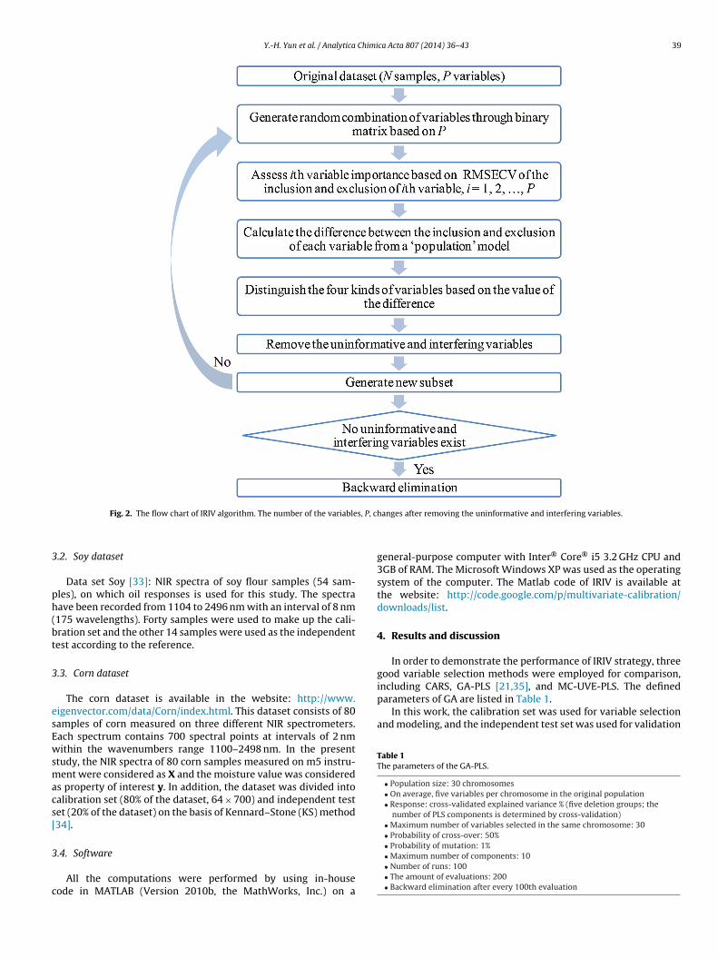

Y.-H. Yun et al. / Analytica Chimica Acta 807 (2014) 36– 43 39

s, P, c

3

ph(bt

3

esEwsmacs[

3

c

including CARS, GA-PLS [21,35], and MC-UVE-PLS. The definedparameters of GA are listed in Table 1.

In this work, the calibration set was used for variable selectionand modeling, and the independent test set was used for validation

Table 1The parameters of the GA-PLS.

• Population size: 30 chromosomes• On average, five variables per chromosome in the original population• Response: cross-validated explained variance % (five deletion groups; the

number of PLS components is determined by cross-validation)• Maximum number of variables selected in the same chromosome: 30• Probability of cross-over: 50%• Probability of mutation: 1%

Fig. 2. The flow chart of IRIV algorithm. The number of the variable

.2. Soy dataset

Data set Soy [33]: NIR spectra of soy flour samples (54 sam-les), on which oil responses is used for this study. The spectraave been recorded from 1104 to 2496 nm with an interval of 8 nm175 wavelengths). Forty samples were used to make up the cali-ration set and the other 14 samples were used as the independentest according to the reference.

.3. Corn dataset

The corn dataset is available in the website: http://www.igenvector.com/data/Corn/index.html. This dataset consists of 80amples of corn measured on three different NIR spectrometers.ach spectrum contains 700 spectral points at intervals of 2 nmithin the wavenumbers range 1100–2498 nm. In the present

tudy, the NIR spectra of 80 corn samples measured on m5 instru-ent were considered as X and the moisture value was considered

s property of interest y. In addition, the dataset was divided intoalibration set (80% of the dataset, 64 × 700) and independent testet (20% of the dataset) on the basis of Kennard–Stone (KS) method34].

.4. Software

All the computations were performed by using in-houseode in MATLAB (Version 2010b, the MathWorks, Inc.) on a

hanges after removing the uninformative and interfering variables.

general-purpose computer with Inter® Core® i5 3.2 GHz CPU and3GB of RAM. The Microsoft Windows XP was used as the operatingsystem of the computer. The Matlab code of IRIV is available atthe website: http://code.google.com/p/multivariate-calibration/downloads/list.

4. Results and discussion

In order to demonstrate the performance of IRIV strategy, threegood variable selection methods were employed for comparison,

• Maximum number of components: 10• Number of runs: 100• The amount of evaluations: 200• Backward elimination after every 100th evaluation

40 Y.-H. Yun et al. / Analytica Chimica Acta 807 (2014) 36– 43

Table 2The results of different methods on the diesel fuels dataset.

Methods nVAR nLVs RMSEC RMSEP

PLS 401 10 3.0643 3.8597GA-PLS 61.0 ± 20.5 8.8 ± 1.4 2.7438 ± 0.1334 3.4113 ± 0.1872

otcb((

4(

swtf

i

i

i

i

i

i

oci

4

tCssITrTt

trfFmow

wtno

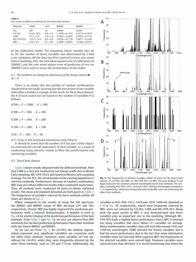
Fig. 3. The frequencies of selected variables within 50 times for the diesel fuelsdataset. (A) GA-PLS; (B) CARS; (C) MC-UVE-PLS; (D) IRIV. The gray shadows in thefigure represent the common selected wavelengths by the four methods. The vari-ables, including 852–854, 1412–1418 and 1454–1456 nm wavelengths (denoted as

CARS 17.1 ± 3.9 7.9 ± 1.4 2.7856 ± 0.1067 3.5022 ± 0.1733MC-UVE-PLS 110.7 ± 51.2 9.8 ± 0.4 2.8538 ± 0.1178 3.4477 ± 0.1367IRIV 47.0 ± 9.5 9.1 ± 0.9 2.3609 ± 0.0591 3.1568 ± 0.0727

f the calibration model. The maximum latent variable was seto 10. The number of latent variables was determined by 5-foldross validation. All the data was first centered to have zero meanefore modeling. Also, the root mean square error of calibration setRMSEC) and the root mean square error of prediction of test setRMSEP) were used to assess the performance of the model.

.1. The problem on setting the dimension of the binary matrix MK × P)

There is no doubt that the number of random combinationshould not be too small, assuring that the interaction of one variableith other variables is enough. In this work, for these three dataset,

he K of each round was set based on the number of variables P asollows:

f 500 = P < 1000, K = 500

f 300 = P < 500, K = 300

f 200 = P < 300, K = 200

f 100 = P < 200, K = 100

f 50 = P < 100, K = 50

f P < 10 go to the backward elimination step (Step 6)It should be noted that the number of K has just a little impact

n assessing the overall importance of each variable, as a result ofonducting many iterative rounds to filter the uninformative andnterfering variables.

.2. Diesel fuels dataset

Table 2 shows results obtained with the different methods. Notehat CARS is a very fast method but not always stable due to Montearlo sampling. MC-UVE-PLS is also based on Monte Carlo samplingtrategy. For GA-PLS, the chromosome of the existing population iselected randomly. Furthermore, because of random combination,RIV may also obtain different results when conducted many times.hus, all methods were conducted 50 times to obtain statisticalesults. The mean and standard deviation are both given in Table 2.he frequencies of variables selected by these methods within 50imes are shown in Fig. 3.

When compared to the results of using the full spectrum,he RMSEC and RMSEP values of IRIV decrease 23% and 18%,espectively. Clearly, IRIV has highly improved the prediction per-ormance with a reduced dimensionality. A boxplot is used inig. 4A for a better display of the prediction performance of the fourethods. From Table 2 and Fig. 4A, we also can observe that IRIV

bviously has the best prediction performance than other methodsith the lowest RMSEC and RMSEP.

As we can see from Fig. 3, for GA-PLS, the shadow regions,

hich represent very significant variables, are consistent with

he other three methods. However, some variables are not sig-ificant for GA-PLS, while they were frequently selected by thether three methods, such as 770 and 772 nm. Additionally, the

1–3, respectively), which were frequently selected by IRIV, were not selected by theother three methods.

variables at 852–854, 1412–1418 and 1454–1456 nm (denoted as1–3 in Fig. 3D, respectively), which were frequently selected byIRIV, were not selected by GA-PLS, CARS and MC-UVE-PLS. Alongwith the good results of IRIV, it was demonstrated that thesevariables play an important role in the modeling. Although MC-UVE-PLS made a slightly better performance than CARS, it selectedtoo many variables that were about 111 variables on average.Many uninformative variables may still exist like around 1522 and1104 nm wavelengths. CARS selected the fewest variables, but ithad the worst performance due to the fact that some informative

variables were not selected. With regard to IRIV, the frequencies ofthe selected variables were overall high. Nineteen variables wereselected more than 40 times. It is worth mentioning that when the

Y.-H. Yun et al. / Analytica Chimica Acta 807 (2014) 36– 43 41

Fig. 4. The boxplot of 50 RMSEP values for the four methods. (A) diesel fuels dataset;(B) soy oil dataset; (C) corn moisture dataset. On each box, the central mark is themti

veCjabv

Iikweesivaa

efwtrwe

Fig. 5. The illustration of strongly informative, weakly informative, uninformativeand interfering variables discriminated by MPA for the diesel fuels dataset; lightblue distributions represent the inclusion of ith variable, while gray distributionsrepresent the exclusion of ith variable. (A) strongly informative variables; (B) weaklyinformative variables; (C) uninformative variables; (D) interfering variables. (For

edian, the edges of the box are the 25th and 75th percentile, the whiskers extendo the most extreme data points are the maximum and minimum, and the “+”plottedndividually represents outliers.

ariables that were selected more than 40 times are used for mod-ling, the RMSEC and RMSEP are 2.6396 and 3.6826, respectively.omparing this result with the one of IRIV, we observe that the

oint effect between the most significant variables and other vari-bles made contributions. Thus, we can say that IRIV can work welly using the random combination to consider the joint effect ofariables.

In addition, it is also interesting to analyze the process ofRIV. IRIV is a strategy that retains both the strongly and weaklynformative variables with iterative rounds. For ith variable, fourinds of variables could be distinguished by MPA and Eqs. (3)–(6)ith the two RMSECV distribution of ˚0 and ˚i (inclusion and

xclusion of ith variable, respectively). Fig. 5 depicts the differ-nces between them. For instance, the variable 1236 nm thatatisfies Eq. (3) (1236 nm, DMEAN < 0 and P value = 4.8 × 10−94)s identified as strongly informative; 1050 nm (DMEAN < 0 and Palue = 0.4332 > 0.05) is weakly informative; 1468 nm (DMEAN > 0nd P value = 0.6489 > 0.05) is uninformative; 1502 nm (DMEAN > 0nd P value = 0.0128 < 0.05) is interfering.

Fig. 6 shows the change in the number of retained variables inach round (out of 50 times) for the three datasets. As for the dieseluels dataset, at the beginning, about half of the original variablesere removed. Due to removing a large number of uninforma-

ive and interfering variables, it drops very fast in the first threeounds, and then appears mild. It converges gradually at 9th roundith 72 strongly and weakly informative variables. After backward

limination, the number of the final selected variables is 42.

interpretation of the references to color in this figure legend, the reader is referredto the web version of this article.)

4.3. Soy oil dataset

The statistical results obtained by conducting the four methods50 times are reported in Table 3, including the mean and standarddeviation values. Fig. 4B clearly exhibits the difference of theresults by means of a boxplot. It can be seen that IRIV performsmuch better than the other three methods. Fig. 7 visually displaysthe frequencies of selected variables of the four methods revealing

their differences. The variables were selected by all methodsaround 1144–1152, 1216–1224, 1552–1560 and 1632–1640 nm(marked by the shadow region). But as for MC-UVE, it selected

42 Y.-H. Yun et al. / Analytica Chimica Acta 807 (2014) 36– 43

Fig. 6. The change in the number of retained informative variables in each round.The 0 value in the X axis represents the number of the variables in the originaldataset.

Table 3The results of different methods on the soy oil dataset.

Methods nVAR nLVs RMSEC RMSEP

PLS 175 8 0.8217 1.2252GA-PLS 14.0 ± 5.6 4.1 ± 0.3 0.7905 ± 0.0113 1.1236 ± 0.0435CARS 11.1 ± 4.8 5.3 ± 0.7 0.8036 ± 0.0258 1.1518 ± 0.0751

m21bvspvvc

4

Prvspaatqbttpme

Fig. 7. The frequencies of selected variables within 50 times on the soy oil dataset.

TT

MC-UVE-PLS 36.5 ± 5.6 7.2 ± 0.9 0.8158 ± 0.0312 1.1507 ± 0.0159IRIV 12.0 ± 2.6 4.5 ± 0.6 0.7789 ± 0.0138 1.0578 ± 0.0316

any uninformative variables like the variables 2288–2296 and344–2360 nm. Regarding to the variables around 1832 and920 nm, they were selected by IRIV more than 10 times but noty the other methods. We believe that these variables may be notery significant when singly considered, but they may have someynergetic effects with other variables improving the predictionerformance. Fig. 6 shows the trend that the number of retainedariables reduces in each round. For the soy oil dataset, it reducesery rapidly in the first three rounds from 175 to 37, and then it has aonvergence that no uninformative and interfering variables exist.

.4. Corn moisture dataset

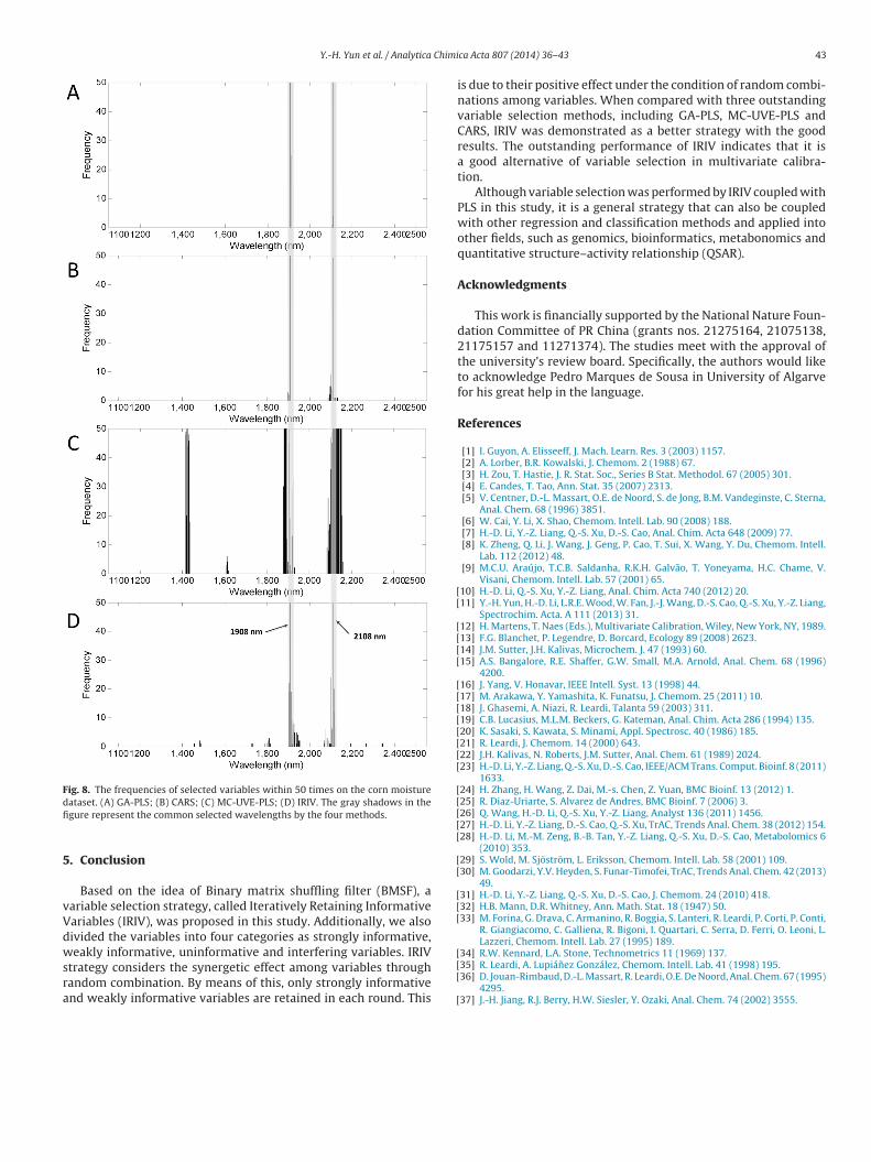
As we did in the first two datasets, GA-PLS, CARS, MC-UVE-LS and IRIV were also conducted 50 times to obtain statisticalesults. Table 4 and Fig. 4C clearly present the results. We canerify that only MC-UVE-PLS performed very badly as a result ofelecting many uninformative variables like 1422–1428 nm. Theerformance of the other methods is nearly the same. The 1908nd 2108 nm wavelengths, which are corresponding to the waterbsorption [36] and the combination of O–H bond [37], were provedo be the key wavelengths in this dataset [7]. Fig. 8 displays the fre-uencies of selected variables of the four methods. From the Fig. 8,oth of them were selected very frequently by all the methods. Fur-hermore, GA and IRIV selected them with 50 times. It can be stated

hat IRIV not only selected the most significant variables but alsoroduced better prediction performance. Additionally, for the coinoisture dataset, the change in the number of retained variables in

ach round is also shown in Fig. 6. It is consistent with the general

able 4he results of different methods on the corn moisture dataset.

Methods nVAR nLVs

PLS 700 9

GA-PLS 3.2 ± 0.7 3.2 ± 0.7

CARS 2.6 ± 1.4 2.5 ± 1.5

MC-UVE-PLS 52.7 ± 4.7 10.0 ± 0

IRIV 7.7 ± 3.6 7.0 ± 3.0

(A) GA-PLS; (B) CARS; (C) MC-UVE-PLS; (D) IRIV. The gray shadows in the figurerepresent the common selected wavelengths by the four methods. Around 1832and 1920 nm wavelengths were selected by IRIV more than 10 times but not by theother methods.

convergence process of the IRIV. The number of retained variables

reduces from 700 to 9, which means that a large amount of vari-ables is not useful. Therefore, it can be said that variable selectionis very important and necessary for multivariate calibration withthe high dimensional data.

RMSEC RMSEP

0.0149 0.02012.8 × 10−4 ± 5.5 × 10−7 3.4 × 10−4 ± 2.7 × 10−6

3.1 × 10−4 ± 3.1 × 10−4 4.0 × 10−4 ± 4.6 × 10−4

3.1 × 10−3 ± 6.9 × 10−4 3.6 × 10−3 ± 8.3 × 10−4

2.6 × 10−4 ± 1.6 × 10−5 3.5 × 10−4 ± 2.5 × 10−5

Y.-H. Yun et al. / Analytica Chimi

Fig. 8. The frequencies of selected variables within 50 times on the corn moisturedfi

5

vVdwsra

[[

[[[[

[[[[[[[[

[[[[[

[[

[[[

ataset. (A) GA-PLS; (B) CARS; (C) MC-UVE-PLS; (D) IRIV. The gray shadows in thegure represent the common selected wavelengths by the four methods.

. Conclusion

Based on the idea of Binary matrix shuffling filter (BMSF), aariable selection strategy, called Iteratively Retaining Informativeariables (IRIV), was proposed in this study. Additionally, we alsoivided the variables into four categories as strongly informative,

eakly informative, uninformative and interfering variables. IRIV

trategy considers the synergetic effect among variables throughandom combination. By means of this, only strongly informativend weakly informative variables are retained in each round. This

[[[

[

ca Acta 807 (2014) 36– 43 43

is due to their positive effect under the condition of random combi-nations among variables. When compared with three outstandingvariable selection methods, including GA-PLS, MC-UVE-PLS andCARS, IRIV was demonstrated as a better strategy with the goodresults. The outstanding performance of IRIV indicates that it isa good alternative of variable selection in multivariate calibra-tion.

Although variable selection was performed by IRIV coupled withPLS in this study, it is a general strategy that can also be coupledwith other regression and classification methods and applied intoother fields, such as genomics, bioinformatics, metabonomics andquantitative structure–activity relationship (QSAR).

Acknowledgments

This work is financially supported by the National Nature Foun-dation Committee of PR China (grants nos. 21275164, 21075138,21175157 and 11271374). The studies meet with the approval ofthe university’s review board. Specifically, the authors would liketo acknowledge Pedro Marques de Sousa in University of Algarvefor his great help in the language.

References

[1] I. Guyon, A. Elisseeff, J. Mach. Learn. Res. 3 (2003) 1157.[2] A. Lorber, B.R. Kowalski, J. Chemom. 2 (1988) 67.[3] H. Zou, T. Hastie, J. R. Stat. Soc., Series B Stat. Methodol. 67 (2005) 301.[4] E. Candes, T. Tao, Ann. Stat. 35 (2007) 2313.[5] V. Centner, D.-L. Massart, O.E. de Noord, S. de Jong, B.M. Vandeginste, C. Sterna,

Anal. Chem. 68 (1996) 3851.[6] W. Cai, Y. Li, X. Shao, Chemom. Intell. Lab. 90 (2008) 188.[7] H.-D. Li, Y.-Z. Liang, Q.-S. Xu, D.-S. Cao, Anal. Chim. Acta 648 (2009) 77.[8] K. Zheng, Q. Li, J. Wang, J. Geng, P. Cao, T. Sui, X. Wang, Y. Du, Chemom. Intell.

Lab. 112 (2012) 48.[9] M.C.U. Araújo, T.C.B. Saldanha, R.K.H. Galvão, T. Yoneyama, H.C. Chame, V.

Visani, Chemom. Intell. Lab. 57 (2001) 65.10] H.-D. Li, Q.-S. Xu, Y.-Z. Liang, Anal. Chim. Acta 740 (2012) 20.11] Y.-H. Yun, H.-D. Li, L.R.E. Wood, W. Fan, J.-J. Wang, D.-S. Cao, Q.-S. Xu, Y.-Z. Liang,

Spectrochim. Acta. A 111 (2013) 31.12] H. Martens, T. Naes (Eds.), Multivariate Calibration, Wiley, New York, NY, 1989.13] F.G. Blanchet, P. Legendre, D. Borcard, Ecology 89 (2008) 2623.14] J.M. Sutter, J.H. Kalivas, Microchem. J. 47 (1993) 60.15] A.S. Bangalore, R.E. Shaffer, G.W. Small, M.A. Arnold, Anal. Chem. 68 (1996)

4200.16] J. Yang, V. Honavar, IEEE Intell. Syst. 13 (1998) 44.17] M. Arakawa, Y. Yamashita, K. Funatsu, J. Chemom. 25 (2011) 10.18] J. Ghasemi, A. Niazi, R. Leardi, Talanta 59 (2003) 311.19] C.B. Lucasius, M.L.M. Beckers, G. Kateman, Anal. Chim. Acta 286 (1994) 135.20] K. Sasaki, S. Kawata, S. Minami, Appl. Spectrosc. 40 (1986) 185.21] R. Leardi, J. Chemom. 14 (2000) 643.22] J.H. Kalivas, N. Roberts, J.M. Sutter, Anal. Chem. 61 (1989) 2024.23] H.-D. Li, Y.-Z. Liang, Q.-S. Xu, D.-S. Cao, IEEE/ACM Trans. Comput. Bioinf. 8 (2011)

1633.24] H. Zhang, H. Wang, Z. Dai, M.-s. Chen, Z. Yuan, BMC Bioinf. 13 (2012) 1.25] R. Diaz-Uriarte, S. Alvarez de Andres, BMC Bioinf. 7 (2006) 3.26] Q. Wang, H.-D. Li, Q.-S. Xu, Y.-Z. Liang, Analyst 136 (2011) 1456.27] H.-D. Li, Y.-Z. Liang, D.-S. Cao, Q.-S. Xu, TrAC, Trends Anal. Chem. 38 (2012) 154.28] H.-D. Li, M.-M. Zeng, B.-B. Tan, Y.-Z. Liang, Q.-S. Xu, D.-S. Cao, Metabolomics 6

(2010) 353.29] S. Wold, M. Sjöström, L. Eriksson, Chemom. Intell. Lab. 58 (2001) 109.30] M. Goodarzi, Y.V. Heyden, S. Funar-Timofei, TrAC, Trends Anal. Chem. 42 (2013)

49.31] H.-D. Li, Y.-Z. Liang, Q.-S. Xu, D.-S. Cao, J. Chemom. 24 (2010) 418.32] H.B. Mann, D.R. Whitney, Ann. Math. Stat. 18 (1947) 50.33] M. Forina, G. Drava, C. Armanino, R. Boggia, S. Lanteri, R. Leardi, P. Corti, P. Conti,

R. Giangiacomo, C. Galliena, R. Bigoni, I. Quartari, C. Serra, D. Ferri, O. Leoni, L.Lazzeri, Chemom. Intell. Lab. 27 (1995) 189.

34] R.W. Kennard, L.A. Stone, Technometrics 11 (1969) 137.35] R. Leardi, A. Lupiánez González, Chemom. Intell. Lab. 41 (1998) 195.36] D. Jouan-Rimbaud, D.-L. Massart, R. Leardi, O.E. De Noord, Anal. Chem. 67 (1995)

4295.37] J.-H. Jiang, R.J. Berry, H.W. Siesler, Y. Ozaki, Anal. Chem. 74 (2002) 3555.