analytic virtual integration for cyber-physical...

3rd Workshop on

Analytic Virtual Integration for

Cyber-Physical Systems

AVICPS 2012

In conjunction with IEEE RTSS, San Juan, Puerto Rico

December 4th, 2012

iii

Chair’s Foreword

Welcome to AVICPS 2012, the 3rd Workshop on Analytical Virtual Integration of Cyber-Physical Systems. The goal of the workshop is to explore architectural design patterns, tools and the theoretical analytical foundations for creating common system-wide composition models, where key properties can be studied and guarantees provided before the start of actual development. The concept of virtual integration has emerged with the advent of model-based development. Models allow us to reason about the system and predict its properties before the system is built. In this way, we can discover design flaws early in the development process, when errors are easier and cheaper to fix. A large fraction of errors in the system design emerge during integration, therefore analyzing integration at the modeling level is of particular importance. Cyber-physical systems (CPS) bring an additional level of complexity to system in general, and to the problem of integration in particular. CPS components may affect each other through digital communication channels, as in any other computer-based system, but also by coupling through the physical world. Physical influence on the digital communication channels has to be considered as well. This year, AVICPS brings together researchers addressing multiple aspects of virtual integration. The workshop includes papers on various modeling approaches for CPS components and system environments, architecture-driven system development, safety analysis, among others. Presentations of contributed papers are supplemented by two keynote talks by Peter Feiler (Software Engineering Institute) and Michael Whalen (University of Minnesota), who bring complementary perspectives on the area. As in the past, AVICPS is held together with the Real-Time Systems Symposium, which keeps us in touch with the larger community of researchers exploring related problems. We are grateful to RTSS organizers for providing this opportunity and handling many essential aspects of the workshop organization. We also acknowledge generous support of the Software Engineering Institute and PRECISE Center at the University of Pennsylvania. Finally, our sincere thanks go to the program committee members. This workshop would not be possible without their time and effort. We hope you will enjoy participating in AVICPS 2012, and making it a success! Sagar Chaki and Oleg Sokolsky

AVICPS 2012 co-Chairs

v

Program Committee:

Rajeev Alur, University of Pennsylvania, USA

Saddek Bensalem, Verimag, France

Ken Butts, Toyota, USA

David Broman, UC Berkeley, USA

Julien Delange, European Space Agency, Netherlands

Jorgen Hansson, Chalmers University, Sweden

Boudewijn Haverkort, Embedded Systems Institute, Netherlands

Jerome Hugues, Institute for Space and Aeronautics Engineering, France

Mirko Jakovljevic, TTTech, USA

Christoph Kirsch, University of Salzburg, Austria

Jens Knoop, TU Vienna, Austria

Bruce Krogh, Carnegie Mellon University, USA

Thomas Noll, RWTH Aachen, Germany

Roman Obermaisser, University of Siegen, Germany

K. C. Shashidhar, Mathworks, USA

Sandeep Shukla, Virginia Tech, USA

Mike Whalen, University of Minnesota, USA

Program Co-Chairs: Oleg Sokolsky, University of Pennsylvania (Penn), USA

Sagar Chaki, Software Engineering Institute (SEI), USA

vii

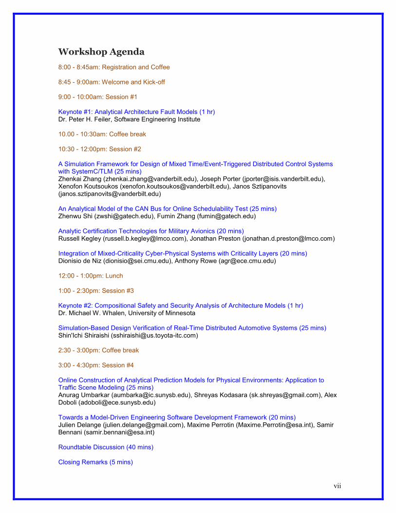
Workshop Agenda

8:00 - 8:45am: Registration and Coffee 8:45 - 9:00am: Welcome and Kick-off 9:00 - 10:00am: Session #1

Keynote #1: Analytical Architecture Fault Models (1 hr) Dr. Peter H. Feiler, Software Engineering Institute 10.00 - 10:30am: Coffee break 10:30 - 12:00pm: Session #2 A Simulation Framework for Design of Mixed Time/Event-Triggered Distributed Control Systems with SystemC/TLM (25 mins) Zhenkai Zhang ([email protected]), Joseph Porter ([email protected]), Xenofon Koutsoukos ([email protected]), Janos Sztipanovits ([email protected]) An Analytical Model of the CAN Bus for Online Schedulability Test (25 mins) Zhenwu Shi ([email protected]), Fumin Zhang ([email protected]) Analytic Certification Technologies for Military Avionics (20 mins) Russell Kegley ([email protected]), Jonathan Preston ([email protected]) Integration of Mixed-Criticality Cyber-Physical Systems with Criticality Layers (20 mins) Dionisio de Niz ([email protected]), Anthony Rowe ([email protected]) 12:00 - 1:00pm: Lunch 1:00 - 2:30pm: Session #3 Keynote #2: Compositional Safety and Security Analysis of Architecture Models (1 hr) Dr. Michael W. Whalen, University of Minnesota Simulation-Based Design Verification of Real-Time Distributed Automotive Systems (25 mins) Shin'Ichi Shiraishi ([email protected]) 2:30 - 3:00pm: Coffee break

3:00 - 4:30pm: Session #4 Online Construction of Analytical Prediction Models for Physical Environments: Application to Traffic Scene Modeling (25 mins) Anurag Umbarkar ([email protected]), Shreyas Kodasara ([email protected]), Alex Doboli ([email protected]) Towards a Model-Driven Engineering Software Development Framework (20 mins) Julien Delange ([email protected]), Maxime Perrotin ([email protected]), Samir Bennani ([email protected])

Roundtable Discussion (40 mins) Closing Remarks (5 mins)

mailto:[email protected]





ix

Keynote Speaker 1

Dr. Peter H. Feiler, Software Engineering Institute

Title: Analytical Architecture Fault Models Abstract: In this talk we summarize challenges in safety-critical software-intensive systems and introduce the concept of an analyzable architecture fault model expressed in SAE AADL and its Error Model Annex standard. We then present its use early in the development life cycle supporting hazard and fault impact analysis, show its ability to provide compositional analysis, discuss the interaction between operational and failure modes, and conclude with an illustration of its use to gain better understanding of the intricacies of desired timing behavior in safety-critical systems. Bio: Peter Feiler is a 27 year veteran and currently a senior member of the Research, Technology, and Systems Solutions (RTSS) program of the Software Engineering Institute (SEI). His current research interest is in improving the quality of safety-critical software-intensive systems, aka. cyber-physical systems, through architecture-centric virtual integration and analysis throughout the development life cycle to complement traditional testing resulting in major reduction in rework and qualification costs. Peter Feiler has been the technical lead and main author of the SAE Architecture Analysis & Design Language (AADL) standard. He has a Ph.D. in Computer Science from Carnegie Mellon.

x

NOTES

xi

NOTES

xii

Keynote Speaker 2

Dr. Michael W. Whalen, University of Minnesota

Title: Compositional Safety and Security Analysis of Architecture Models Abstract: This talk presents a design flow and supporting analysis tools for compositional analysis of system architectures. We focus on system architecture models composed from libraries of components and complexity-reducing design patterns with formally verified properties. This allows new system designs to be developed rapidly using patterns that have been shown to reduce unnecessary complexity and coupling between components. Components and patterns are annotated with formal contracts describing their guaranteed behaviors and the contextual assumptions that must be satisfied for their correct operation. We describe the compositional reasoning framework that we have developed for proving the correctness of a system design, and illustrate it with an example based on an aircraft flight control system. Bio: Dr. Michael Whalen is the Program Director at the University of Minnesota Software Engineering Center. Dr. Whalen is interested in formal analysis, language translation, testing, and requirements engineering. He has developed simulation, translation, testing, and formal analysis tools for Model-Based Development languages including Simulink, Stateflow, SCADE, and RSML-e, and has published more than 30 papers on these topics. He has led successful formal verification projects on large industrial avionics models, including displays (Rockwell-Collins ADGS-2100 Window Manager), redundancy management and control allocation (AFRL CerTA FCS program) and autoland (AFRL CerTA CPD program).

xiii

NOTES

xiv

NOTES

xv

Abstracts: A Simulation Framework for Design of Mixed Time/Event-Triggered Distributed Control Systems with SystemC/TLM

Zhenkai Zhang ([email protected]), Joseph Porter ([email protected]), Xenofon Koutsoukos ([email protected]), Janos Sztipanovits ([email protected])

Mixed time/event-triggered (TT/ET) distributed control systems are complex systems which have emerged in many cyber-physical domains but have been difficult to evaluate at early design stages. In order to reveal design flaws as early as possible, this paper proposes a simulation framework based on an executable virtual platform model in SystemC/TLM. The executable platform is generated using a model-based approach from a system designed in the Embedded Systems Modeling Language (ESMoL). The virtual platform consists of three types of abstract models, the RTOS model, the communication system model, and the hardware model, to capture different behaviors of the mixed TT/ET distributed control systems. Preliminary results from a case study using a Quadrotor flight control system are used to illustrate the approach.

An Analytical Model of the CAN Bus for Online Schedulability Test Zhenwu Shi ([email protected]), Fumin Zhang ([email protected])

Controller area network (CAN) is a prioritybased bus that supports real-time communication. Existing schedulability analysis for the CAN bus is peformed at the design stage, by assuming that all message information is known in advance. However, in pratice, the CAN bus may run in a dynamic environment, where complete specifications may not be available at the design stage and operational requirements may change at system run-time. In this paper, we develop an analytical model that describes the dynamics of message transmission on the CAN bus. Based on this analytical timing model, we then propose an online test that effectively checks the schedulability of the CAN bus, in the presence of online adjustments of message streams. Simulations show that the online test can accurately report the loss of scheduability on the CAN bus.

Analytic Certification Technologies for Military Avionics

Russell Kegley ([email protected]), Jonathan Preston ([email protected]) Historic approaches to upgrading the capabilities of military aircraft by inserting new technologies have become so costly that warfighters may be forced to operate with less than current technology can deliver. Even inserting new upgrades alongside the legacy systems can be very expensive if it requires large modifications to legacy software, triggering extensive retest. A way to meet this challenge is to insert upgrades alongside legacy systems, virtually replacing old capabilities with new while leaving the old software in place. This approach carries with it new challenges which might be met with analytic innovations.

Integration of Mixed-Criticality Cyber-Physical Systems with Criticality Layers

Dionisio de Niz ([email protected]), Anthony Rowe ([email protected])

Large Cyber-Physical Systems such as avionics and automotive systems often require large integration efforts etween third-party components. These components provide functionality at different levels of criticality yet share many of the same underlying resources (CPU, Memory, Network, Disk, Transducers). As a result, protections mechanisms are needed to prevent lower-criticality task from interfering with higher-criticality ones. In this paper, we discuss how traditional temporal protection mechanisms such ARIC 653 partitions fail to fully protect high-criticality tasks






xvi

from lower-criticality ones. We then show how the Zero-Slack QRAM scheduler (ZSQRAM) can be used in multi-layer systems to avoid these problems. Furthermore, we propose the use of criticality layers based on the asymmetric protection scheme of ZS-QRAM in order to simplify this integration, increase its robustness, and reduce its resource usage. Finally, we discuss some open issues that need to be addressed in order to remove some of the limitations of this approach.

Simulation-Based Design Verification of Real-Time Distributed Automotive Systems

Shin'Ichi Shiraishi ([email protected])

In this paper, we propose a simulation-based verification technique for real-time distributed automotive systems. The proposed technique enables accurate simulation and it utilizes only limited information that can be collected in the design phases of development. In other words, the proposed technique enables the design verification of automotive systems. Therefore, the proposed design verification during early phases of development can potentially enhance the productivity of automotive systems. Moreover, the proposed technique is developed by extending the modeling fundamentals of a single commercial tool known as OPNET Modeler. This tool is widely used in the network technology domain, and it has been provided with sufficient technical support by its vendor. Thus, the proposed method is now available for immediate application to real-world automotive system development.

Online Construction of Analytical Prediction Models for Physical Environments: Application to Traffic Scene Modeling

Anurag Umbarkar ([email protected]), Shreyas Kodasara ([email protected]), Alex Doboli ([email protected])

This paper presents a methodology to model the dynamics of traffic scenes, including the participating vehicles, vehicle clusters, the attributes and relations of the scene elements, and related events, like cluster merging and splitting. Compared to other methods, this methodology constructs the models online using data coming from sensors. The main steps are to identify the elements of a scene, to find the relations among the elements, and to construct analytical prediction models for the traffic scene dynamics. The paper discusses all the related theoretical aspects, including ontologies for traffic scene description, stochastic prediction of event sequences, and vehicle and cluster identification using sound-based vehicle localization.

Towards a Model-Driven Engineering Software Development Framework

Julien Delange ([email protected]), Maxime Perrotin ([email protected]), Samir Bennani ([email protected])

Design and Implementation of Safety-Critical Systems is becoming very difficult becauses it involves many requirements coming from different engineering domains. Due to the increase of complexity, software of such systems can no longer be produced with traditional methods, which show their limit over time. In that context, new development approaches have to be introduced to avoid actual development traps and pitfalls. Among them, the Model-Driven Engineering approach consists at representing system artifacts with models and autogenerate the code by refining them from high-level concepts down to the code. However, as for every new approach, it also brings new problems such as requirements consistency among the different notations (models) as well as integration issues (for example, making sure that implementation code from different models will behave correctly when merged on a single execution platform). This article presents our experience for integrating Guidance and Navigation Control (GNC) algorithms designed with Application Models (Simulink) with Architecture Models (AADL). The process relies on code generator for both models and integrate it on a typical execution platform. In particular, we focus on the challenges of the integration, illustrating the practical problems we faced for producing a space system using a Model-Driven Engineering Approach.

xvii

NOTES

xviii

NOTES

xix

NOTES

Simulation-Based Design Verification of Real-Time Distributed Automotive Systems

Shin’ichi SHIRAISHI

TOYOTA InfoTechnology Center, U.S.A., Inc.465 Bernardo Avenue

Mountain ViewCA 94043

Email: [email protected]

Abstract—In this paper, we propose a simulation-based veri-fication technique for real-time distributed automotive systems.The proposed technique enables accurate simulation and itutilizes only limited information that can be collected in thedesign phases of development. In other words, the proposedtechnique enables the design verification of automotive sys-tems. Therefore, the proposed design verification during earlyphases of development can potentially enhance the productivityof automotive systems. Moreover, the proposed technique isdeveloped by extending the modeling fundamentals of a singlecommercial tool known as OPNET Modeler. This tool is widelyused in the network technology domain, and it has beenprovided with sufficient technical support by its vendor. Thus,the proposed method is now available for immediate applicationto real-world automotive system development.

Keywords-Automotive Systems, System Design Verification,Simulation, Real-Time Systems, Controller Area Network,OPNET Modeler

I. INTRODUCTION

Automotive systems are highly complex distributed em-bedded systems. For example, a certain luxurious car em-ploys several automotive systems constructed on the basisof complex networks wherein nearly 100 electronic controlunits (ECUs) are interconnected. In order to efficientlydevelop such complex systems, system design verification isrequired during the early phases of development. Moreover,the upcoming automotive safety standard (ISO 26262 [1])stipulates that design phase verification is required to ensurehigh-level functional safety.

In spite of such a high demand for early-phase verifi-cation in real-world automotive system development, thereis no straightforward approach to design verification. Thisdrawback is particularly critical in software development;hence, early-phase verification before the implementationphase is not possible without prototyping. Unfortunately,existing techniques cannot simultaneously deal with thevarious aspects of automotive systems, such as, (1) real-timesystems, (2) complex distributed systems based on networks,and (3) cost-sensitive system development.

Regarding the first aspect, most automotive systems arereal-time systems; an accurate analysis is required in terms

of the timeliness. The timeliness of automotive systems isusually verified by using cycle-accurate simulation tech-niques with instruction set simulators. This type of simula-tion is generally known as virtual prototyping, and it requiressoftware implementation, i.e., a set of source code. Althoughvirtual prototyping allows us to avoid hardware prototyping,it does not enable the design-phase verification of software.Virtualization can also be achieved using virtual platforms.Virtual platforms enable us to implement software withoutany RTL descriptions of its execution platform (hardware);however, it requires a set of source code.

The second aspect implies that most automotive systemsare highly distributed systems based on multiple intercon-nected ECUs. In other words, for design verification, it is notsufficient to consider only the software used in automotivesystems, and its execution platform (hardware part), includ-ing microcontrollers, RAMs, and ROMs. Such hardware andsoftware components are the main verification objectives insimulations based on virtual prototyping or virtual platforms;however, the network component of automotive systems isbeyond their scope. Thus, we need an end-to-end verificationtechnique for the network component, which interconnectsthe ECUs, hardware, and software.

The third aspect reflects the strict cost constraint onautomotive system development. This implies that car man-ufacturers (OEMs) cannot afford to implement all the nec-essary development techniques as in-house tools. Thus, weneed to effectively use commercial tools that support early-phase verification, and exploit technical support from theirvendors. A recent paper [2] proposes a holistic simulationtechnique for automotive systems; however, its pragmaticapplication is unlikely because it does not offer any toolimplementation. Another recent paper [3] presents a co-simulation technique based on multiple simulation tools.Despite the advantages of such techniques, they are notconsidered practical from the viewpoint of the purchase andmaintenance cost of multiple commercial tools.

Therefore, in this paper, we try to overcome the afore-mentioned drawbacks and develop a novel design veri-fication technique for automotive systems using a single

commercial tool. More precisely, we propose a high-levelmodeling approach to the holistic simulation of real-timedistributed automotive systems. The proposed technique cansimultaneously simulate the detailed behavior of the threetypes of components: software, hardware, and networks; itutilizes only the limited information available in the designphases. Thus, the proposed simulation technique enablesseveral end-to-end analyses that are essential for the veri-fication of real-time systems. In addition, we can evaluatethe performance of systems under development in theirdesign phases. Such early performance estimation facilitatessystem design verification; hence, the proposed techniquecan potentially enhance the quality and productivity ofautomotive systems. In addition, the proposed techniquedepends only on a single commercial tool that is widely usedin the network technology domain. Therefore, this techniquehas the potential for rapid deployment among stakeholdersinvolved in automotive system development.

II. REAL-WORLD EXAMPLE: REAL-TIME DISTRIBUTED

AUTOMOTIVE SYSTEMS

In this section, we present a real-world example ofcomplex automotive systems. Through this case study, weclarify the difficulties related to the design verification ofautomotive systems.

A. Automotive Systems Based on Complex In-Vehicle Net-works

Figure 1 shows an in-vehicle controller area network(CAN) [4] of a certain luxurious car in the Japanese market.Three CAN buses are interconnected via a gateway ECU(hereafter, referred to as a GW ECU), and each CAN bushas 10–20 ECUs. Over this large-scale network, more than200 types of messages are exchanged. The network shownin Fig. 1 is a part of the entire structure of networks inthe sampled car. In general, luxury-class cars have approxi-mately 100 ECUs that are interconnected by 10 buses suchas CAN and LIN (local interconnect network) [5] buses.This implies that besides the GW ECU shown in Fig. 1,luxurious cars have several types of GW ECUs with differentspecifications. For example, one GW ECU bridges differentspeed buses such as 250 kbps and 500 kbps; another GWECU bridges different protocols such as CAN and LIN, andso on.

Networks in which several ECUs are interconnected serveas platforms that support various real-time automotive sys-tems such as adaptive cruise control systems, vehicle dy-namics integrated management systems, and pre-crush safetysystems. For example, an adaptive cruise control systemrequires an engine control ECU, a skid control ECU, and aradar sensor ECU; these ECUs must be interconnected via anetwork. Simultaneously, the pre-crush safety system utilizesthe same components. Similarly, numerous components areshared among several different systems; thus, networks

V Bus

...

...

...

Gateway

ECU

ECU CAN BUS

Suspension

Control

Steering

Control

Engine

Control

ECU 3A

ECU 2A

ECU 1A

Steering Bus

Chassis Bus

Figure 1. Distributed Automotive Systems (CAN-based Network).

and GW ECUs are typical components shared by multiplesystems.

To summarize, a new end-to-end analysis technique isrequired for shared components such as networks and GWECUs for the purpose of system design verification, whichis required by the ISO 26262 standard.

B. Architecture of CAN–CAN Gateway ECU

When we discuss design verification of automotive sys-tems, we need to focus on the fact that GW ECUs areimportant components for system design verification. Asmentioned earlier, most automotive systems are real-timesystems; hence, we need to analyze the timeliness of suchsystems in an end-to-end manner. On the other hand, delaysproduced by GW ECUs have a significant impact on end-to-end analysis; however, the early estimation of end-to-enddelays is complicated owing to the complex functionalitiesof GW ECUs. Paradoxically, this means that GW ECUs areideal subjects for discussing design verification in detail;hence, they are central to this paper, hereafter. It should benoted that the following discussion can be applied to othertypes of ECUs.

Figure 2 shows the architecture of the GW ECU shown inFig. 1. This figure indicates that the GW ECU is equippedwith priority control in order to realize end-to-end QoS man-agement. Moreover, a computation-intensive functionality,i.e., routing, is realized by hardware, whereas the others areimplemented by software. This design decision is motivatedby a trade-off between the latency and the flexibility of theGW ECU. This implies that design verification must be aco-verification of hardware and software. In addition to thehardware and software components, some buffers are locatedat the borders among hardware, software, and networks. Thebehavior analysis of these buffers, such as a buffer overflowor underflow, is critical to design verification.

III. POTENTIAL APPROACHES TO SYSTEM

VERIFICATION AND THEIR DRAWBACKS

There exist two potential approaches to system design ver-ification: an analytical (formal) approach and a simulation-based approach. The analytical approach is effective in in-vestigating corner cases. If we apply the analytical approach

RX

Register

V

RX

Register

Steering

RX

Register

Chassis

Routing

Logic

FIFO

FIFO

FIFO

TX

Register

TX

Register

TX

Register

V

Steering

Chassis

Priority

Control

Priority

Control

Priority

Control

Hardware Software

Figure 2. Architecture of Multi-Channel CAN Gateway ECU.

to the GW ECU discussed in Sect. II, we can estimate themaximum delay, maximum buffer usage, etc. On the otherhand, the simulation-based approach can be adopted forperformance analyses. For example, we can estimate severalperformance parameters such as mean delays and averagebuffer utilization. Both these approaches are important forsystem design verification because they can be appliedto different design subphases. Although we are actuallyinvestigating the analytical approach, we will focus on thesimulation-based approach in the remainder of this paperowing to space constraints1.

Reviewing the discussions in Sect. II, a system designverification technique must be able to handle the followingtwo types of behavior.

1) Inter-ECU behavior: The interconnection of ECUs vianetworks.

2) Intra-ECU behavior: The interaction between the hard-ware and the software within ECUs.

In the following sections, we will discuss two different typesof approaches that can potentially handle the two behaviorsstated above.

A. Network-oriented Approach

The first potential approach to system design verificationis to use network simulation technologies. This approachseems to be able to perform end-to-end analysis of automo-tive systems. Network simulation tools, e.g., OPNET Mod-eler [7], enable us to simulate the network component, i.e.,CAN, LIN buses, etc. Unfortunately, such a simulation isnot sufficient for the holistic analysis of complex automotivesystems such as the one shown in Fig. 1. As discussed inSect. II, the GW ECU shown in Fig. 1, which interconnectsmultiple CAN buses, provides complex functionalities viasoftware. More precisely, it enables priority control as shownin Fig. 2. Thus, it is not feasible to simplify the GW ECUinto a simple delay element that can be easily handled bynetwork simulators. In other words, network simulators can-not replicate the detailed behavior of the GW ECU, whichis dominant in design verification and must be analyzedthrough simulation.

1See [6] for details of our research on the analytical approach.

System Design

SystemArchitecture

Task

Work Product

Hardware Design

HadwareArchitecture

Software Design

SoftwareArchitecture

Hardware Implementation

RTL

Software Implementation

Source Code

SoC

ROM

Compiler

Compiler

Virtual Platform

Virtual Prototyping

System

Objective of This Paper

IntegrationDesign Phase ImplementationFigure 3. Workflow of Hardware and Software Co-Design with HardwareVirtualization.

B. Hardware Virtualization Approach

The second potential approach is to use co-verificationtechniques with hardware virtualization that have been es-tablished in the ESL (electronic system-level) field. Forexample, the internal behavior of ECUs is usually ana-lyzed via cycle-accurate techniques featuring instruction setsimulators, e.g., CoMET [8]. This type of technique isknown as virtual prototyping, and its typical workflow isshown in Fig. 3. Virtual prototyping is useful for timelinessverification of systems under development. However, it isclear from Fig. 3 that virtual prototyping can be applied onlyto test phases because it requires implemented software, i.e.,a set of source code. Unfortunately, the cost of eliminatingdefects in test phases is much higher that in design phases.Furthermore, unlike network simulators, virtual prototypingcannot enable end-to-end analysis of systems while consid-ering network components such as CAN and LIN buses.

Virtualization can also be achieved using virtual plat-forms. Although virtual platforms enable system verificationbased on a hardware design, software implementation isrequired. On the other hand, the objective of this paper is toachieve system design verification based on both hardwareand software design specifications.

C. Co-simulation Approach

Co-simulation [3] is another potential approach to systemdesign verification. Combining the two techniques describedabove would be possible from a technical point of view.This approach can enable end-to-end analysis based on thedetailed behavior of ECUs. However, the co-simulation ap-proach is not considered pragmatic because it uses multipletools for the same verification and it involves high runningcosts.

As discussed in Sects. III-A and III-B, existing techniquesare insufficient for the realization of design verification ofautomotive systems. Thus, a new verification technique isrequired to deal with the combination of hardware, software,and networks. On the other hand, future automotive systemswill be not be standalone systems, and their connectivitywill be mandatory. Thus, from the viewpoint that multiple

Network Topology

Node

Protocol Stack within Node

Processor

State Machine of Process

Procedure within State

State

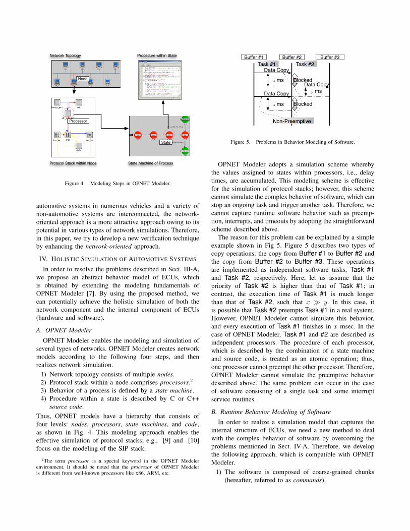
Figure 4. Modeling Steps in OPNET Modeler.

automotive systems in numerous vehicles and a variety ofnon-automotive systems are interconnected, the network-oriented approach is a more attractive approach owing to itspotential in various types of network simulations. Therefore,in this paper, we try to develop a new verification techniqueby enhancing the network-oriented approach.

IV. HOLISTIC SIMULATION OF AUTOMOTIVE SYSTEMS

In order to resolve the problems described in Sect. III-A,we propose an abstract behavior model of ECUs, whichis obtained by extending the modeling fundamentals ofOPNET Modeler [7]. By using the proposed method, wecan potentially achieve the holistic simulation of both thenetwork component and the internal component of ECUs(hardware and software).

A. OPNET Modeler

OPNET Modeler enables the modeling and simulation ofseveral types of networks. OPNET Modeler creates networkmodels according to the following four steps, and thenrealizes network simulation.

1) Network topology consists of multiple nodes.2) Protocol stack within a node comprises processors.2

3) Behavior of a process is defined by a state machine.4) Procedure within a state is described by C or C++

source code.Thus, OPNET models have a hierarchy that consists offour levels: nodes, processors, state machines, and code,as shown in Fig. 4. This modeling approach enables theeffective simulation of protocol stacks; e.g., [9] and [10]focus on the modeling of the SIP stack.

2The term processor is a special keyword in the OPNET Modelerenvironment. It should be noted that the processor of OPNET Modeleris different from well-known processors like x86, ARM, etc.

Buffer #1 Buffer #2 Buffer #3

Data Copy

Non-Preemptive

x ms

x ms

Data Copy

Data Copy

Task #1 Task #2

y ms

Blocked

Blocked

Figure 5. Problems in Behavior Modeling of Software.

OPNET Modeler adopts a simulation scheme wherebythe values assigned to states within processors, i.e., delaytimes, are accumulated. This modeling scheme is effectivefor the simulation of protocol stacks; however, this schemecannot simulate the complex behavior of software, which canstop an ongoing task and trigger another task. Therefore, wecannot capture runtime software behavior such as preemp-tion, interrupts, and timeouts by adopting the straightforwardscheme described above.

The reason for this problem can be explained by a simpleexample shown in Fig 5. Figure 5 describes two types ofcopy operations: the copy from Buffer #1 to Buffer #2 andthe copy from Buffer #2 to Buffer #3. These operationsare implemented as independent software tasks, Task #1and Task #2, respectively. Here, let us assume that thepriority of Task #2 is higher than that of Task #1; incontrast, the execution time of Task #1 is much longerthan that of Task #2, such that x � y. In this case, itis possible that Task #2 preempts Task #1 in a real system.However, OPNET Modeler cannot simulate this behavior,and every execution of Task #1 finishes in x msec. In thecase of OPNET Modeler, Task #1 and #2 are described asindependent processors. The procedure of each processor,which is described by the combination of a state machineand source code, is treated as an atomic operation; thus,one processor cannot preempt the other processor. Therefore,OPNET Modeler cannot simulate the preemptive behaviordescribed above. The same problem can occur in the caseof software consisting of a single task and some interruptservice routines.

B. Runtime Behavior Modeling of Software

In order to realize a simulation model that captures theinternal structure of ECUs, we need a new method to dealwith the complex behavior of software by overcoming theproblems mentioned in Sect. IV-A. Therefore, we developthe following approach, which is compatible with OPNETModeler.

1) The software is composed of coarse-grained chunks(hereafter, referred to as commands).

Initiation

Idle

Command

Queueing

Command

End

Command

Start

State

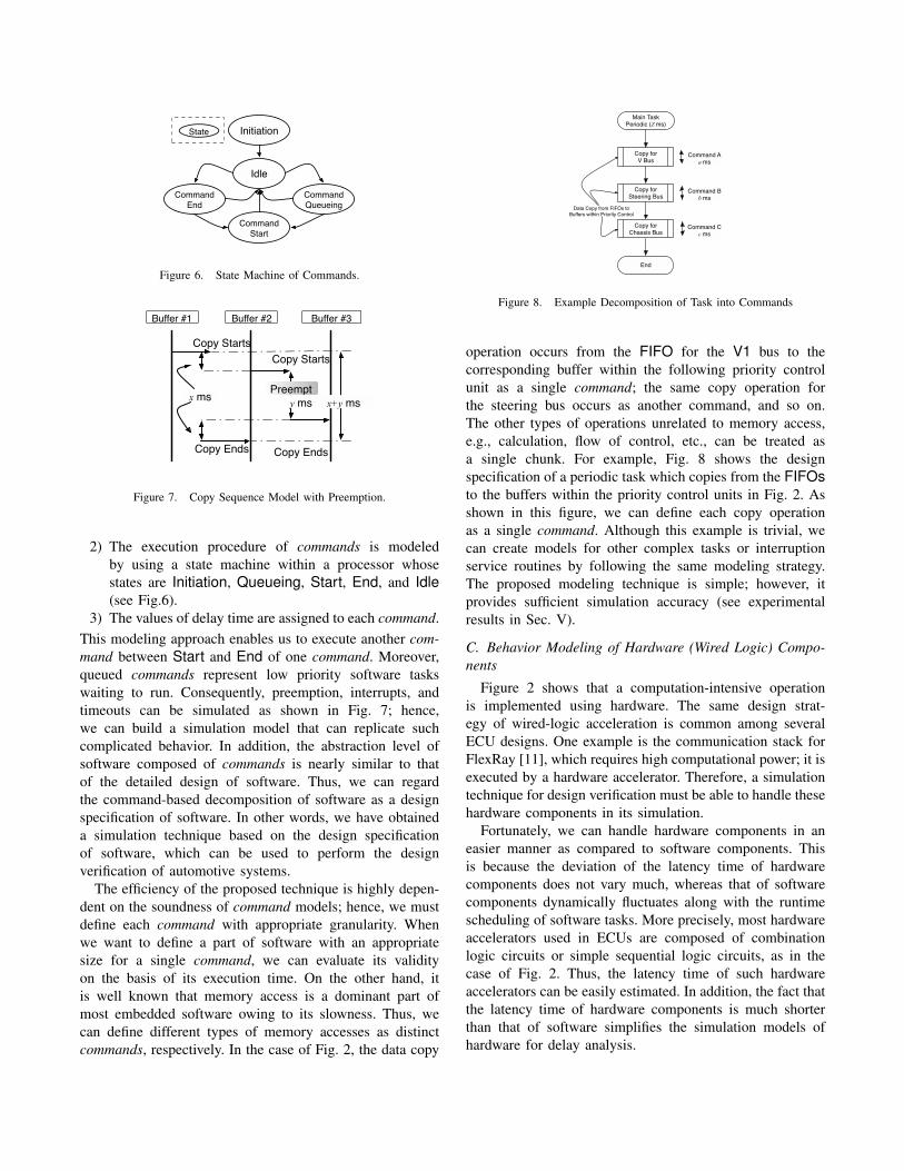
Figure 6. State Machine of Commands.

Buffer #1 Buffer #2 Buffer #3

Copy Starts

Copy Ends Copy Ends

Copy Starts

Preempt

y msx ms

x+y ms

Figure 7. Copy Sequence Model with Preemption.

2) The execution procedure of commands is modeledby using a state machine within a processor whosestates are Initiation, Queueing, Start, End, and Idle(see Fig.6).

3) The values of delay time are assigned to each command.This modeling approach enables us to execute another com-mand between Start and End of one command. Moreover,queued commands represent low priority software taskswaiting to run. Consequently, preemption, interrupts, andtimeouts can be simulated as shown in Fig. 7; hence,we can build a simulation model that can replicate suchcomplicated behavior. In addition, the abstraction level ofsoftware composed of commands is nearly similar to thatof the detailed design of software. Thus, we can regardthe command-based decomposition of software as a designspecification of software. In other words, we have obtaineda simulation technique based on the design specificationof software, which can be used to perform the designverification of automotive systems.

The efficiency of the proposed technique is highly depen-dent on the soundness of command models; hence, we mustdefine each command with appropriate granularity. Whenwe want to define a part of software with an appropriatesize for a single command, we can evaluate its validityon the basis of its execution time. On the other hand, itis well known that memory access is a dominant part ofmost embedded software owing to its slowness. Thus, wecan define different types of memory accesses as distinctcommands, respectively. In the case of Fig. 2, the data copy

Main TaskPeriodic (Z ms)

End

Copy for V Bus

Copy for Steering Bus

Copy for Chassis Bus

Data Copy from FIFOs to

Buffers within Priority Control

Command Aa ms

Command Bb ms

Command Cc ms

Figure 8. Example Decomposition of Task into Commands

operation occurs from the FIFO for the V1 bus to thecorresponding buffer within the following priority controlunit as a single command; the same copy operation forthe steering bus occurs as another command, and so on.The other types of operations unrelated to memory access,e.g., calculation, flow of control, etc., can be treated asa single chunk. For example, Fig. 8 shows the designspecification of a periodic task which copies from the FIFOsto the buffers within the priority control units in Fig. 2. Asshown in this figure, we can define each copy operationas a single command. Although this example is trivial, wecan create models for other complex tasks or interruptionservice routines by following the same modeling strategy.The proposed modeling technique is simple; however, itprovides sufficient simulation accuracy (see experimentalresults in Sec. V).

C. Behavior Modeling of Hardware (Wired Logic) Compo-nents

Figure 2 shows that a computation-intensive operationis implemented using hardware. The same design strat-egy of wired-logic acceleration is common among severalECU designs. One example is the communication stack forFlexRay [11], which requires high computational power; it isexecuted by a hardware accelerator. Therefore, a simulationtechnique for design verification must be able to handle thesehardware components in its simulation.

Fortunately, we can handle hardware components in aneasier manner as compared to software components. Thisis because the deviation of the latency time of hardwarecomponents does not vary much, whereas that of softwarecomponents dynamically fluctuates along with the runtimescheduling of software tasks. More precisely, most hardwareaccelerators used in ECUs are composed of combinationlogic circuits or simple sequential logic circuits, as in thecase of Fig. 2. Thus, the latency time of such hardwareaccelerators can be easily estimated. In addition, the fact thatthe latency time of hardware components is much shorterthan that of software simplifies the simulation models ofhardware for delay analysis.

RX

Register

V (500 kbps)

RX

Register

MS (250 kbps)

Priority

Control

FIFO

FIFO

TX

Register

TX

Register

V

MS

Software

Figure 9. Architecture of Dual-Channel CAN Gateway ECU.

Actually, in the GW ECU architecture in Fig. 2, thehardware component, which executes routing operations,produces constant latency from the RxRegisters to theFIFOs, unless simultaneous receptions of multiple messagesfrom different buses occur. This means that we only haveto consider such conflict conditions in simulation. Hence,we can calculate the delay of a certain message from thecorresponding RxRegister to FIFO by simply multiplyingthe latency time of the non-conflict case, i.e., two or threetimes longer when simultaneously receiving from two orthree buses, respectively.

According to the aforementioned modeling strategy, OP-NET Modeler can simulate the internal behavior of ECUswhile considering both hardware and software. Furthermore,OPNET Modeler is inherently able to simulate CAN buses,which interconnects multiple ECUs, in a straightforwardmanner. Eventually, combining the three types of models,i.e., the software model, hardware model, and networkmodel, we can perform an exhaustive holistic simulation ofautomotive systems using a single tool (OPNET Modeler).

V. EXPERIMENTAL RESULTS

In this section, we present some experimental results toverify the effectiveness of the proposed holistic simulationtechnique. In the experiments, two different types of GWECUs are used (see Table I). The first gateway (GW ECU#1) is identical to the GW ECU shown in Fig. 2. Thesecond one (GW ECU #2) connects two CAN buses withdifferent speeds, and its architecture is shown in Fig. 9. Thesimulation results of the proposed technique are comparedwith those of conventional virtual prototyping using CoMET.

Figures 10(a) and 10(b) show the simulation (OPNET)models obtained by applying the proposed technique to thesetwo GW ECUs. These simulation models enable severaltypes of analyses from the following viewpoints.(1) Message delay.

• Delay in buffers and GW ECUs.• End-to-end delay.

(2) Buffer utilization.• Average buffer utilization.

Table ISPECIFICATIONS OF TARGET GATEWAY ECUS.

Name GW ECU #1 GW ECU #2

Type CAN–CAN CAN–CAN

Channels 3 channels 2 channels

Buses V, Steering, and Chassisbuses

V and MS buses

Bus Speed 500 kbps 500 kbps (V) and 250kbps (MS)

Logic Hardware & Software Software

Architecture Figure 2 Figure 9

• Buffer overflow and underflow.• Maximum buffer usage and minimum buffer usage.

(3) Message lost.Regarding message delay, comparisons between the pro-

posed OPNET-based simulation and CoMET-based simula-tion are provided below. Figures 11 and 12 show com-parisons of the mean message delays estimated using theproposed technique and CoMET-based simulation. Moreprecisely, Figs. 11(a) and 12(a) illustrate the estimated GWdelays that are equivalent to the latency between messagereception in RX registers and transmission from TX regis-ters. Figs. 11(b), 11(c), 12(b), and 12(c) partially showthe breakdown of the GW delays: estimated delays in RXregisters and FIFOs.

In these figures, we can find some deviations of thedelays estimated by the two approaches; however, they areapproximately less than 20% in most cases. In particular,the proposed technique provides equivalent accuracy in thecases of important messages with high priorities. In addition,comparing Figs. 11 and 12, we can recognize that theproposed technique can achieve high accuracy, irrespectiveof the architectures of simulation targets (see Figs. 2 and 9).

Figures 13(a) and 13(b) show comparisons of estimatedend-to-end delays, which is the latency time between mes-sage transmission from source ECUs and reception in sinkECUs. This end-to-end delay analysis was infeasible whenwe used only CoMET-based simulation; however, they werefeasible using the proposed holistic simulation technique.

From the viewpoints of buffer utilization such as overflow,underflow, and maximum usage, and message lost, theresults obtained by using both the simulations are identical.This implies that the deviations of the simulation resultsshown in Figs. 11 and 12 do not have any impact on thearchitecture decisions of the GW ECUs.

Based on the discussion presented above, the proposedtechnique provides sufficient accuracy despite its coarsegranularity. Moreover, the proposed technique enables anend-to-end delay analysis, unlike the CoMET-based tech-nique. Besides the accuracy, the simulation speed of the pro-posed method also enhances its effectiveness. The proposed

!

Gateway ECU #1

V Bus

Steering Bus

Chassis Bus

(a) GW ECU #1 and CAN buses.

Gateway ECU #2

V Bus

MS Bus

(b) GW ECU #2 ECU and CAN buses.

Figure 10. OPNET Models of Distributed Automotive Systems.

��

��

��

��

��

�� !�"�#$%��& ��'��!��(�&�)$

(a) Mean GW Delay.

��

��

��

��

��

��

��

��

�� ! ��"�#�$%& ��' ��(��"��)�'�*%�

(b) Mean Delay in Rx Register

��

��

��

��

��

�� !�"�#$%��& ��'��!��(�&�)$

(c) Mean Delay in FIFO.

Figure 11. Comparisons between Simulation Results of OPNET andCoMET Models (GW ECU #1).

simulation technique is around 1.5 times faster than execu-tion in a real-time environment, even under an ordinary PCenvironment (Intel Core 2 Duo 2.33GHz); such accelerationcannot be expected in the case of fine-grained simulationsuch as virtual prototyping.

Summarizing the quantitative discussion presented aboveon the basis of the experimental results and the qualitative

��

��

��

��

��

��

��

�� !"� �#�$�%&'��( ��)� �#� �*�(�+&�

(a) Mean GW Delay.

��

��

��

��

��

��

��

�� ! ��"�#�$%& ��' ��(��"��)�'�*%�

(b) Mean Delay in Rx Register

��

��

��

��

��

��

�� !�"�#$%��& ��'��!��(�&�)$

(c) Mean Delay in FIFO.

Figure 12. Comparisons between Simulation Results of OPNET andCoMET Models (GW ECU #2).

��

��

��

��

��

��

�� !�"#

(a) Simulation Results of GW ECU #1.

��

��

��

��

��

��

��

�� !"

(b) Simulation Results of GW ECU #2.

Figure 13. End-to-End Delay Estimated by Proposed Technique.

discussion presented in Sects. III and IV, we derive acomparison between the proposed technique and CoMET-based simulation, as shown in Table II. The table showsthat each approach has different characteristics, and hence,different applicable phases. This implies that we can useboth approaches in a collaborative way for different typesof verification, i.e., the proposed technique is used fordesign verification, and CoMET-based simulation is used forimplementation verification.

Table IICOMPARISON BETWEEN PROPOSED AND COMET-BASED SIMULATION.

Approaches Proposed CoMET-Based

Coverage Software, hardware,and network

Software and hardware

Abstraction High Low

Design models (e.g.Fig. 8)

Source code (softwareand hardware)

Accuracy Medium High

Simulation Speed High Medium

Applicable Phase Design Test

Required Literacy C language C language and HDL

System Design

SysML Model

Task

Work Product

Hardware Design

MARTE Model

Software Design

MARTE Model

OPNET Model

Translation

Co-Design Co-Verification

Simulation

Figure 14. Model-Based Development using Proposed OPNET-basedSimulation (Future Work).

VI. CONCLUSION AND FUTURE WORK

In this paper, we proposed an OPNET-based simulationof real-time distributed automotive systems. The proposedtechnique can deal with the three important componentsof automotive systems, i.e., hardware and software withinECUs, and networks among ECUs. Thus, it enables a holisticsimulation of automotive systems. Moreover, the end-to-endanalysis is a new feature enabled by the proposed holisticsimulation, which was infeasible when we used CoMET-based simulation. The proposed technique enables designverification; hence, the efficiency of system development canbe potentially enhanced by using this technique. In addition,the proposed technique depends on a single commercial tool;hence, it has low running costs and it can be immediatelydeployed for real-world development.

In the future, it will be necessary to ensure that theproposed technique conforms with standardized modelingmethods, e.g., SysML, MARTE, etc. Once the alignmentwith these standards is established, model-based develop-ment in close collaboration with the proposed simulationtechnique should be possible, as shown in Fig.14.

VII. ACKNOWLEDGEMENT

The author would like to extend his gratitude to Fu-miyuki KAGARA (Toyota Technical Development), Hiroki

KONDO and Naoki OHTA (CIJ) for their contribution.

REFERENCES

[1] ISO/DIS 26262 Road vehicles – Functional safety –.ISO/TC22/SC3/WG16, June 2009.

[2] C. Lauer, R. German, and J. Pollmer, “Discrete event simula-tion and analysis of timing problems in automotive embeddedsystems,” in Systems Conference, 2010 4th Annual IEEE,2010, pp. 18 –22.

[3] M. Karner, E. Armengaud, C. Steger, and R. Weiss, “Holisticsimulation of flexray networks by using run-time modelswitching,” in Design, Automation Test in Europe ConferenceExhibition (DATE), 2010, 2010, pp. 544 –549.

[4] CAN Specification Version 2.0. R. Bosch GmbH, September1991.

[5] LIN Specification Package Revision 2.0. LIN Consortium,September 2003.

[6] M. Sebastian, P. Axer, R. Ernst, N. Feiertag, and M. Jersak,“Efficient reliability and safety analysis for mixed-criticalityembedded systems,” in the SAE World Congress, 2011, pp.544 –549, to be published.

[7] OPNET Modeler. http://www.opnet.com.

[8] CoMET. http://www.synopsys.com.

[9] H. Atrianfar and Z. Ayatollahi, “Expansion of OPNET mod-eler’s SIP model for performance evaluation of hierarchicalcall routing in NGN,” in International Conference on Scien-tific Computing (ICSC 2008), 2008, pp. 179 –185.

[10] T. Le, S. Cook, G. Kuthethoor, P. Sesha, G. Hadynski, D. Ki-wior, and D. Parker, “Performance analysis for SIP basedVoIP services over airborne tactical networks,” in AerospaceConference, 2010 IEEE, 6-13 2010, pp. 1 –8.

[11] FlexRay Communications System Protocol Specification Ver-sion 2.1. FlexRay Consortium, May 2005.

A Simulation Framework for Design of MixedTime/Event-Triggered Distributed Control Systems

with SystemC/TLMZhenkai Zhang, Joseph Porter, Xenofon Koutsoukos, and Janos Sztipanovits

Institute for Software Integrated Systems (ISIS)Department of Electrical Engineering and Computer Science

Vanderbilt UniversityNashville, Tennessee, USA

Email: {zhenkai.zhang, joseph.porter, xenofon.koutsoukos, janos.sztipanovits}@vanderbilt.edu

Abstract—Mixed time/event-triggered (TT/ET) distributedcontrol systems are complex systems which have emerged inmany cyber-physical domains but have been difficult to evaluateat early design stages. In order to reveal design flaws as earlyas possible, this paper proposes a simulation framework basedon an executable virtual platform model in SystemC/TLM. Theexecutable platform is generated using a model-based approachfrom a system designed in the Embedded Systems ModelingLanguage (ESMoL). The virtual platform consists of three typesof abstract models, the RTOS model, the communication systemmodel, and the hardware model, to capture different behaviors ofthe mixed TT/ET distributed control systems. Preliminary resultsfrom a case study using a Quadrotor flight control system areused to illustrate the approach.

Keywords-Mixed Time/Event-Triggered Distributed ControlSystems; Virtual Platform; SystemC/TLM; Graphical Models;

I. INTRODUCTION

Nowadays, most complex cyber-physical systems (CPSs),such as automotive vehicles, air planes and trains, use dis-tributed control systems, in which several ECUs are connectedby network(s)/bus(es) [22]. Typically, these control systemsare hard real-time systems. Traditionally, these control sys-tems are composed of event-triggered (ET) tasks and useevent-triggered communication systems, such as CAN bus.As time-triggered architectures (TTA) offer advantages suchas determinism, predictability, and composability [9], manynew systems tend to be built using TTA. However, manysporadic events make the designs not fit into the strict periodicframework [13]. These CPS control systems often consistof both TT and ET tasks and use a mixed communicationprotocol (e.g. FlexRay and TTEthernet) to form mixed TT/ETdistributed control systems [17].

When designing mixed TT/ET distributed control systems,many challenges arise due to a large design space and lack oftools to explore it. First, the hardware platform needs to be de-signed including a set of nodes connected by a communicationsystem. Trade-offs between cost and performance drive theselection of the appropriate processors. The communicationsystem bandwidth and topology also need to be considered

in order to meet performance and redundancy requirements.Then, partitioning tasks into TT or ET needs to be considered.Moreover, mapping the tasks on the hardware platform is alsoimportant and affects timing [17]. After mapping, the mixedcommunication system needs to be configured using properparameters. Thus, the space of possible design configurationsis large and early evaluation is necessary to eliminate baddesign decisions which may cause the system to fail to meetits requirements at a later design stage. However, most existingwork focuses on specifying the control system [23], analyz-ing the system’s schedulability [18], optimizing partitioning,mapping and bus cycle [17], and inter-task communicationmechanism [21], but not evaluating the whole system.

For mixed TT/ET distributed control systems, both com-putation and communication should be captured to enableevaluation of the whole system with respect to functionality,timing, and performance. Both computation and communica-tion concerns are coupled to the application software, systemsoftware and hardware platform. The ability to model, inte-grate, and simulate all parts together is essential for designspace exploration during early development. A virtual platformincluding both hardware and embedded software can be usedas a pivot in this evaluation framework, since it is availablemuch earlier than the real system [7].

System-Level Design Languages (SLDLs), such as SystemCand SpecC, can be used to model both hardware platformsand embedded software. In addition, most SLDLs support theconcept of transaction-level modeling (TLM) which separatesthe design of the computation and communication. A TLMcommunication structure abstracts away communication de-tails to speed up simulation while keeping required accuracy.SystemC has been a de facto SLDL [3]. It also has a TLMlibrary for modeling memory-mapped buses. SystemC/TLM-based virtual platforms on system-level can model the hard-ware behavior with good simulation efficiency and sufficienttiming accuracy at early stages [4].

In order to evaluate a mixed TT/ET system, we pro-pose a simulation framework based on a virtual platform inSystemC/TLM and is combined with a model-based design

environment in GME [12]. The virtual platform consists of amixed TT/ET computation model and communication model.For the computation model, an abstract RTOS model andabstract hardware models such as processor and peripheralsare needed. The abstract RTOS model is built in SystemCand takes charge of task scheduling, inter-task communication,synchronization and interrupt handling [5] [11] [24]. Thebehaviors of both TT and ET tasks should be captured bythe abstract RTOS model, and abstract hardware models formthe underlying computational platform. For the communicationmodel, an abstract communication system model which cancapture the behaviors of both TT and ET communication isneeded. Since FlexRay has been widely used in many CPSdomains, it is a good reference for modeling the mixed TT/ETcommunication [2]. The abstract communication system modelin this framework is based on FlexRay.

The simulation framework is also integrated with a model-based design environment in GME called Embedded SystemsModeling Language (ESMoL) [19]. The mixed TT/ET dis-tributed control systems in ESMoL can be transformed tothe virtual platform models using automated model transfor-mations. This integration makes the design and simulationof the mixed TT/ET systems effective and efficient. As theframework is still in progress, preliminary results from a casestudy using a Quadrotor flight control system are used toillustrate the approach. The bandwidth of two communicationsystems is evaluated for the designed mixed TT/ET system.

There have been efforts to establish simulation frameworksfor design of distributed real-time control systems. In [15],a framework based on generated virtual execution platformis proposed, in which VaST tool is used to model a cycle-accurate hardware platform and µC/OS-II RTOS is ported tothe modeled platform. Although the simulation can be veryaccurate, the very low abstraction level makes it not suitablefor early design evaluation. Compared to [15], a frameworknamed E-TTM is proposed on a very high abstraction level forthe design of TTA-based real-time control systems in [16]. Toohigh level of abstraction also impedes the use of the frameworkdue to inaccuracy. In [14], a UML-based design framework isproposed. A system is described in UML, and then the UMLmodel can be converted into SystemC model for simulation.However, this framework is only for TT applications withoutconsidering mixed TT/ET systems.

Compared to the related efforts, the main contributions ofthis proposed framework are: (1) it uses abstract computationand communication models to establish a universal simulationframework for mixed TT/ET systems, while the levels ofabstraction are appropriate to keep the simulation efficient andaccurate; (2) the framework is also integrated with a model-based design tool to improve its usability.

The rest of this paper is organized as follows: Section 2introduces the virtual platform model in the proposed sim-ulation framework which consists of three types of models;Section 3 describes how to transform an ESMoL designinto an executable virtual platform; Section 4 gives a casestudy on the design of a Quadrotor flight control system

and uses the simulation framework to evaluate the influenceof the bandwidths of the communication systems; Section 5concludes this paper and gives future work.

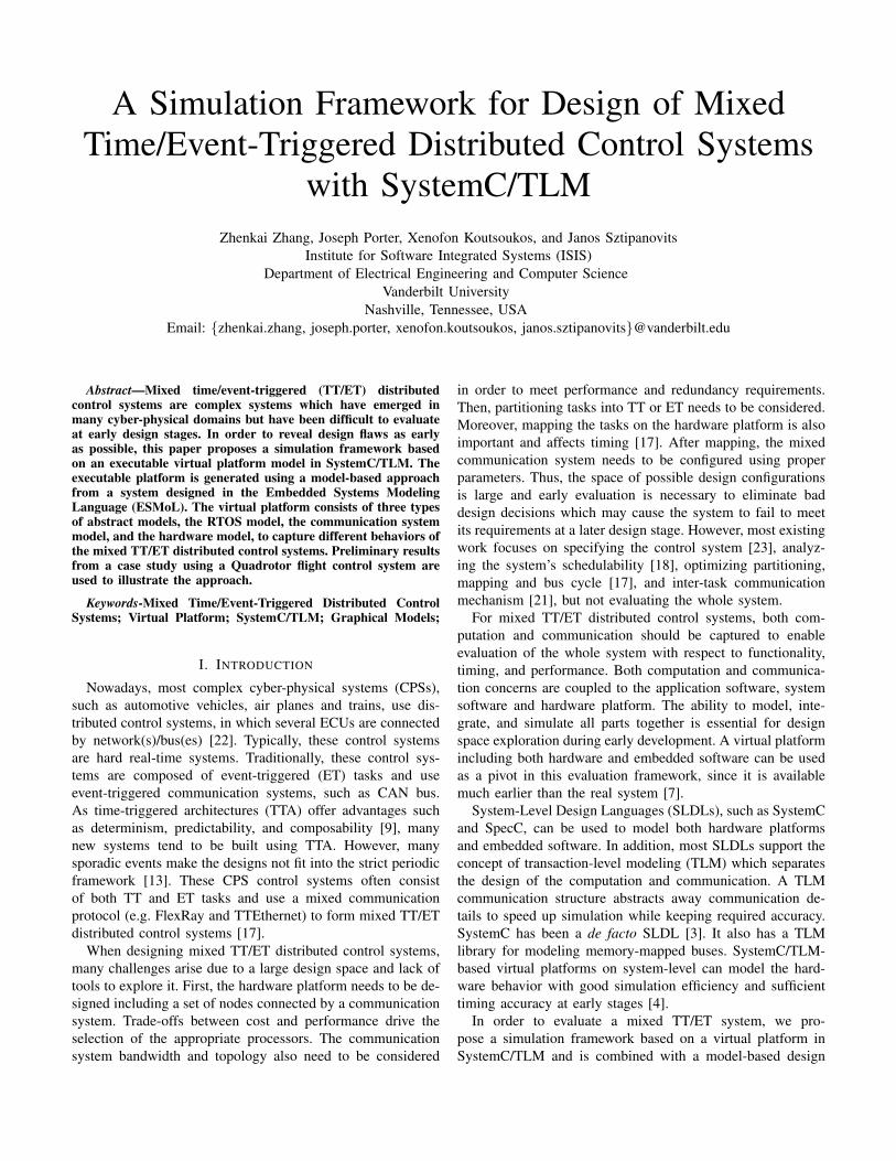
II. VIRTUAL PLATFORM MODEL

Fig. 1. Virtual platform with abstract RTOS model, abstract communicationsystem model, and abstract hardware model.

The virtual platform, as shown in Fig. 1, consists of threetypes of models which are the abstract RTOS model, the ab-stract hardware model, and the abstract communication systemmodel. The models are implemented in SystemC by inheritingfrom the sc module class in which concurrent behaviors aremodeled by a set of SystemC processes (SC THREAD orSC METHOD). These three models can be instantiated andintegrated to be an executable model for simulating mixedTT/ET control systems.

A. RTOS Modeling

On a node of a distributed system, TT and ET tasks whichrealize the desired functionalities interact with an RTOS. TheRTOS captures the dynamic behaviors of the tasks.

The abstract RTOS model has three SC THREAD processes,which are the RTOS service process interacting with TT andET tasks, the time-trigger process taking charge of triggeringTT tasks according to a static schedule, and the interrupthandling process invoking an interrupt service routine (ISR)to handle the corresponding interrupt. Fig. 2 shows the funda-mental services supported by the abstract RTOS model.

1) Task Management: In a mixed TT/ET system, tasksare divided into TT tasks and ET tasks. Time-triggered tasksare activated according to a predefined schedule. When anode’s synchronized local clock reaches a predefined timeinstant, the corresponding TT task will be put into the readyqueue. TT tasks can be non-preemptive or preemptive. ETtasks are activated dynamically depending on the occurrenceof associated events. ET tasks can also be non-preemptive orpreemptive.

Each task in the abstract RTOS model corresponds toa SystemC SC THREAD process. In order to serialize thetasks and control their execution, each task pends on its ownsc event object. The RTOS scheduler controls the executionby notifying the task’s sc event object. A task’s execution

Fig. 2. Abstract RTOS model with supported primitives

information is stored in its Task Control Block (TCB). Sincein SystemC the execution between two wait() statements isin zero simulation time, we need to advance time and modelexecution of tasks by using wait() statements. The executiontime of a section of code is modeled by inserting timingannotations into the task. The annotation can be coarse-grainedon the task level or fined-grained on the basic block orstatement level.

There are a set of primitives provided by the RTOS modelto manage a task’s creation, termination, resumption and sus-pension. When created, each task needs a task name, a worstcase execution time (WCET), and a deadline. In addition,each TT task also needs a predefined schedule passed as aparameter, and each event-triggered task needs a user-definedpriority and/or a period depending on the scheduling policy.

2) Scheduling: The scheduler is the heart of the RTOS,which allocates CPU time to a selected task from the readyqueue. The scheduler’s behavior depends on a specific schedul-ing algorithm. In the abstract RTOS model, the scheduler hasthree common priority-based scheduling policies which arerate monotonic (RM), deadline monotonic (DM), or earliestdeadline first (EDF). Other scheduling algorithms can also beeasily added into the RTOS model. The scheduler’s timingproperties are RTOS- and hardware platform-specific. Basi-cally, there are two main parameters of its timing properties:scheduling overhead and context switching overhead. Thereis some research work on how to accurately acquire theseparameters [6] [8], which is not the focus of this paper, so weassume the parameters are already available for a particularsystem.

The task state transitions are modeled by two finite statemachines as shown in Fig. 3, one for TT tasks and theother one for ET tasks. The Created state is for any newtask. Depending on the task type (TT or ET), it transitions

to the corresponding state. A TT task enters the Idle state,and an ET task enters the Ready state. A TT task enters theReady state statically according to an a priori schedule table,while an ET task enters the Ready state dynamically when theevent happens. There is only one ready queue, which containsboth time-triggered and event-triggered “ready-to-run” tasks.The scheduler schedules this ready queue using the assignedscheduling policy. Only one task can be in the Running stateat a time which is chosen by the scheduler.

Fig. 3. Task state transitions of TT/ET tasks.

3) Inter-Task Communication: In a multi-tasking RTOS,tasks need to communicate with others synchronously orasynchronously using inter-task communication mechanisms.In the abstract RTOS model, inter-task communication on onenode can be achieved by shared memory or message queue,and inter-task communication between different nodes can beachieved by message-passing. Shared memory is used betweenTT tasks, since it can be accessed without race-conditions.Semaphore synchronization is used by ET tasks to serializeaccess to shared memory and maintain task dependencies.

Communication between TT and ET tasks on a single nodeoccurs through message queue. An agent is associated with aTT task in the message queue as a state message keeper. Ifthe message queue is empty, when an ET task tries to poll amessage from it, it will be blocked on it; whereas, for a TTtask, the agent will give the task the message in the queue ifit is available, and then update its state message as the latestdequeued message or give the task the state message if thequeue is empty. So when a TT task accesses the messagequeue, it will never be blocked even if there is no messageavailable in the queue.

Communication between two tasks on different nodes arethrough message passing. Two types of messages are sup-ported in the model, one is TT and the other one is ET. TTmessages are transmitted in the predefined static time slots of acommunication cycle. ET messages are transmitted accordingto the combination of their priorities and the dynamic slots.

4) Interrupt Handling: SystemC has some disadvantagesfor RTOS modeling, which can be summarized as non-interruptible wait-for-delay time advance and non-preemptivesimulation processes. When an interrupt happens, it requiresthe real-time system to react and handle it in a timely manner.Modeling an accurate interrupt handling mechanism plays animportant role in RTOS modeling. We adopt the method from

[24] which makes task use wait-for-event other than wait-for-delay to advance its execution time. A system call of the RTOSmodel taking execution time as its argument makes the taskwait on a sc event object which will be notified after thegiven execution time elapses if no interrupt happens. Whenan interrupt happens and its corresponding ISR preempts theexecution of the task, the notification of the sc event objectwill be canceled and a new notification time will be calculatedaccording to how much time the preemption took and howmuch execution time already passed.

B. Communication System Modeling

In a distributed control system, the timing behavior of thecommunication system has an important impact on systemperformance. There are a few communication protocols thatprovide predictable message delays [20]. The abstract commu-nication system model in this framework is based on FlexRayprotocol [2], which can handle both time-triggered and event-triggered communication. The data granularity of the modelis at the message-level, since we only need to considermessage delay rather than the detailed timing of underlyingoperations for evaluation of the system. The behavior of thecommunication system is modeled by a state chart as shownin Fig. 4. The abstract communication system model takesadvantage of the global time in the SystemC simulation kernel,and uses it as its synchronized time base.

The communication controller model realizes the behavioralmodel of the communication system and takes charge oftransmitting and receiving messages through the underlyingmedium. Its implementation class is also derived from thesc module class of SystemC. It also utilizes the TLM-2.0library in SystemC to realize the underlying transmission.The TLM-2.0 library is mainly for modeling memory-mappedbuses, so we change some of its semantics to model ourcommunication system. The controller acts as both an initiatorand a target for TT/ET bus transactions, and the TT/ET busis an interconnect component. The controller also acts as atarget for memory-mapped bus transactions within a node.The write command of a transaction means to transmit themessage included in the generic payload. For simplicity, onlythe blocking transport interface (b transport() method) is used.

Bus communication is organized in cycles. Each cycleconsists of three segments including a time-triggered staticsegment, an event-triggered dynamic segment and a waitingsegment. The time-triggered part is based on a time-divisionmultiple-access (TDMA) medium access protocol (MAC), andthe event-triggered part is based on flexible TDMA as inFlexRay and Byteflight [2] [1]. For time-triggered communica-tion, a predefined schedule is also needed and passed througha configuration file.

In the static segment superstate, if the current time slot isscheduled to receive a message from the bus, the communi-cation controller goes into RECV state; if scheduled to senda message, it transitions to the SEND state to start a messagetransmission. Otherwise, it will stay in the IDLE state. When astatic time slot is elapsed, the model checks whether the time-

Fig. 4. Behavior of the abstract communication system model based onFlexRay protocol.

triggered communication part is finished by comparing if theslot counter has reached the allocated number of static slots.The schedule guarantees there are no transmission contentions,so dynamic arbitration is not necessary.

The dynamic segment superstate takes charge of event-triggered communication. The segment is divided into a set ofminislots. A frame ID variable is updated synchronously byevery node in the system. In order to solve the contentions be-tween sending nodes, the rights of transmission are ordered bythe frame ID assigned to each node. Different from FlexRay,in this model the dynamic messages are put in a single queue.The queue is sorted by the priorities assigned to the messagesassociated with the task’s priorities, and the messages with thesame priority are ordered by FIFO. Each dynamic time slot canhave varying number of minislots. The length of a dynamictime slot depends on the size of the transmitted message. Whenthe controller transmits the data in its queue, the controllerneeds to check whether this is allowed. First, it checks if ithas the right to use the current frame ID by comparing withits assigned frame IDs. Then, it searches in the queue forthe message with the highest priority which can fit into theremaining dynamic segment time. If there is such a message,the controller sends it on the bus by calling b transport()method; otherwise, the controller defers sending and will tryin the next cycle. When the dynamic communication phase isfinished, the controller enters the WAIT state. In FlexRay, thistime is mainly for clock synchronization. Since we use theglobal time in the SystemC simulation kernel, we do not needto do clock synchronization and we use this state to model arealistic timing behavior.

C. Hardware Modeling

The abstract RTOS model is running on an abstract proces-sor model which communicates with other peripherals througha memory-mapped bus modeled in TLM-2.0, as shown in Fig.1. Peripherals are divided into communication controllers andother I/O devices. I/O devices are used to model sensors andactuators that interact with the plant dynamics. Each I/O devicehas a corresponding ISR SC THREAD process in the RTOSregistered when calling RegisterDevice(). In the current stateof the framework, the processor is modeled in a simplifiedway. The abstract RTOS model interacts with the processormodel by: (1) the tasks invoke ReadMsg(), WriteTTMsg(), andWriteETMsg() primitives to make the processor initiate bustransactions with the communication controller; (2) the pro-cessor signals the RTOS model that a registered I/O device’sISR needs to be activated; (3) the ISR signals the processor tostart bus transactions with the corresponding I/O devices. Theprocessor model has a sc port object which is a multi-portconnected by each I/O device’s interrupt request (IRQ) wire.

Each I/O device is derived from the sc module class andhas a SC THREAD process to control its IRQ behavior. Thebehavior of the IRQ can be modeled in two modes, asyn-chronously periodic and sporadic. For example, an UART’sIRQ can be modeled as sporadic if the interval between twointerrupts has a minimum period, or it can be modeled asasynchronously periodic if the interrupts have a fixed periodbut are not synchronized with the clock of the processor.When an IRQ occurs, the I/O device will trigger the IRQwire connected to the processor and corresponding ISR willbecome ready to handle the IRQ. The ISR will be put intothe ready queue first usually with the highest priority, then itwould preempt other tasks and run immediately. The order ofinterrupt handling is based on the IRQ priorities if there aremore than one IRQs at the same time. When an ISR finishes,it will check if there is any ET task pending on it and putthe corresponding blocked task into the ready queue. EachI/O device also has a SC THREAD process to interact withthe plant model. If the device is a sensor, a sense process willpull sensor data from the plant and wait for a read transaction.If the device is an actuator, an actuate process will wait for awrite transaction and send the data to the plant.

III. MODEL-BASED APPROACH

The front end of this simulation framework is a singlemulti-aspect embedded software design environment calledEmbedded Systems Modeling Language (ESMoL) [19]. Theexecutable simulation model is generated from ESMoL. Themodel transformation process is shown in Fig. 5. Two inter-preters are used to realize the model transformations.

An ESMoL model consists of different models used to cap-ture different aspects of the designed system. The design entryof an ESMoL model is to specify the control system’s func-tionality in the Simulink environment. The Simulink modelwill be imported into the ESMoL automatically to become thefunctional specification for instances of software components.

A logical software architecture model is established to cap-ture data dependencies between software component instancesindependent of their distribution over different processors. Ahardware platform model is defined hierarchically as hardwareunits with ports for interconnections. By mapping softwarecomponents to processing nodes and data messages to com-munication ports, a deployment model is created. By attachingtiming parameter blocks to components and messages, a timingmodel is established. The whole design process is describedin detail in [19].

The interpreter in stage 1 transforms the ESMoL model toan equivalent model in an intermediate language called ES-MoL Abstract. The model in this intermediate language is flat-tened and the relationships implied by structures in ESMoL arerepresented by explicit relation objects in ESMoL Abstract.This translation is similar to the way a compiler translatesconcrete syntax first to an abstract tree, and then to interme-diate semantic representations suitable for optimization. Theinterpreter in stage 2 uses the UDM model navigation API togenerate the simulation model according to the correspondingtemplates. The generation of the simulation model consists ofthree parts.

Fig. 5. ESMoL model and its corresponding SystemC model via modeltransformation using two interpreters.

The first part is to instantiate the hardware and softwaremodels according to the templates. Each processor, I/O de-vice, communication controller, bus, and RTOS in the ES-MoL Abstract model is instantiated in the sc main() function.All the instances belonging to the same node are assembledby binding the sockets or ports. The communication controllerin each node is bound to the TT/ET bus instance. Each I/Odevice is registered into the RTOS by calling RegisterDevice()

method, which will register an ISR SC THREAD processwith its timing and type information (sensor/actuator) passedthrough the ESMoL model. ISR process pends on its ownsc event object, and has the address information of the device.Each task has a corresponding SC THREAD process. Theprocess pends on its own sc event object which will be notifiedif the process is chosen to run by the scheduler. A task istime-triggered if its ExecInfo object in the ESMoL modelis a TTExecInfo object, whereas it is event-triggered if itsExecInfo object is a AsyncPeriodicExecInfo or a SporadicEx-ecInfo object. A TT task only waits on its own sc eventobject. An ET task waits on the corresponding event by callingeither WaitOnDevice, WaitOnSemaphore or WaitOnMsgQueueprimitive. When the event occurs, the ET task goes to theready queue. All the tasks are registered into the RTOSinstances by calling either CreateTTTask() (time-triggered) orCreateETTask() (event-triggered) primitive. If the task is asender of a message, it invokes WriteTTMsg() system call tosend a TT message, or WriteETMsg() if the message is an ETone. Shared variables are used for inter-task communication ofthe same task type (TT/ET). Communication channel betweena TT task and an ET task on the same node in the ESMoLmodel is translated to a message queue. The plant model alsohas a SC THREAD process for time stepping its dynamicsfunction and is instantiated in the sc main() function. Thisprocess also exchanges data with sensors/actuators via sharedmemory.

The second part generates the configuration files for themodel instances according to the specified attributes in theESMoL model, such as the static schedule tables for RTOSesand the segment configurations for communication controllers.The third part is to generate the functional C code for the tasksand the plant dynamics using Real-Time Workshop (RTW),and integrate the functional code with the generated model inthe first part. The generated codes can be easily wrapped intothe corresponding SC THREAD processes of the tasks and theplant model.

IV. CASE STUDY

In this section, we employ the simulation framework for thedesign of a Quadrotor flight control system and present somepreliminary results to illustrate the approach.

The controller for the Quadrotor is designed using two linearproportional derivative (PD) controllers, an inner loop and anouter loop, as shown in Fig. 6. The outer loop controller is

Fig. 6. Two PD controllers in the Quadrotor control system.

a “slow” PD inertial controller and the inner loop is a “fast”

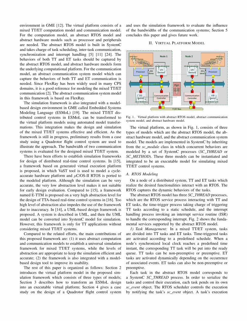
PD attitude controller. More details are described in [10]. Thecorresponding Simulink model (shown in Fig. 7) is built whichhas four blocks (ReferenceHandler, DataHandler, InnerLoopand OuterLoop). After validation of the Simulink model, themodel is automatically imported into ESMoL.

Fig. 7. Simulink model of the Quadrotor control system.

Four ESMoL models are established to capture differentaspects of the design. As shown in Fig. 8, the logical softwarearchitecture in the ESMoL model gives the data dependenciesof the tasks in the Quadrotor control system. Fig. 9 showsthe platform of the Quadrotor which has two nodes, one isbased on PXA255 processor and the other one is based onATmega128, and they are connected by a TT/ET bus. Eachnode has its I/O devices to interact with the outside plant.For task deployment as shown in Fig. 10, two tasks (Ref-erenceHandler and OuterLoop) are assigned to the PXA255node, and the other two tasks (DataHandler and InnerLoop)are assigned to the ATmega128 node. A timing model (Fig.11) is also established by attaching timing parameter blocksto components and messages. As shown in Fig. 11, theReferenceHandler task and DataHandler task are assignedas event-triggered tasks, and the other two tasks are time-triggered tasks.

In this design, we constrain the design space by usingthe above hardware platform, task type (TT/ET) assignment,and task deployment, and only focus on the influence of thebandwidth of the TT/ET bus.

Fig. 8. Software data dependencies of the Quadrotor control system.

The sampling period of the system is 20ms. For tasks oneach node, their WCETs are measured empirically. On thePXA255 processor, ReferenceHandler needs 50µs with rela-tive deadline 5ms, and OuterLoop needs 1.6ms with relativedeadline 2ms. On the ATmega128 processor, DataHandlerneeds 200µs with relative deadline 4ms, and InnerLoop needs600µs with relative deadline 1ms. The ISR of the Ethernet on

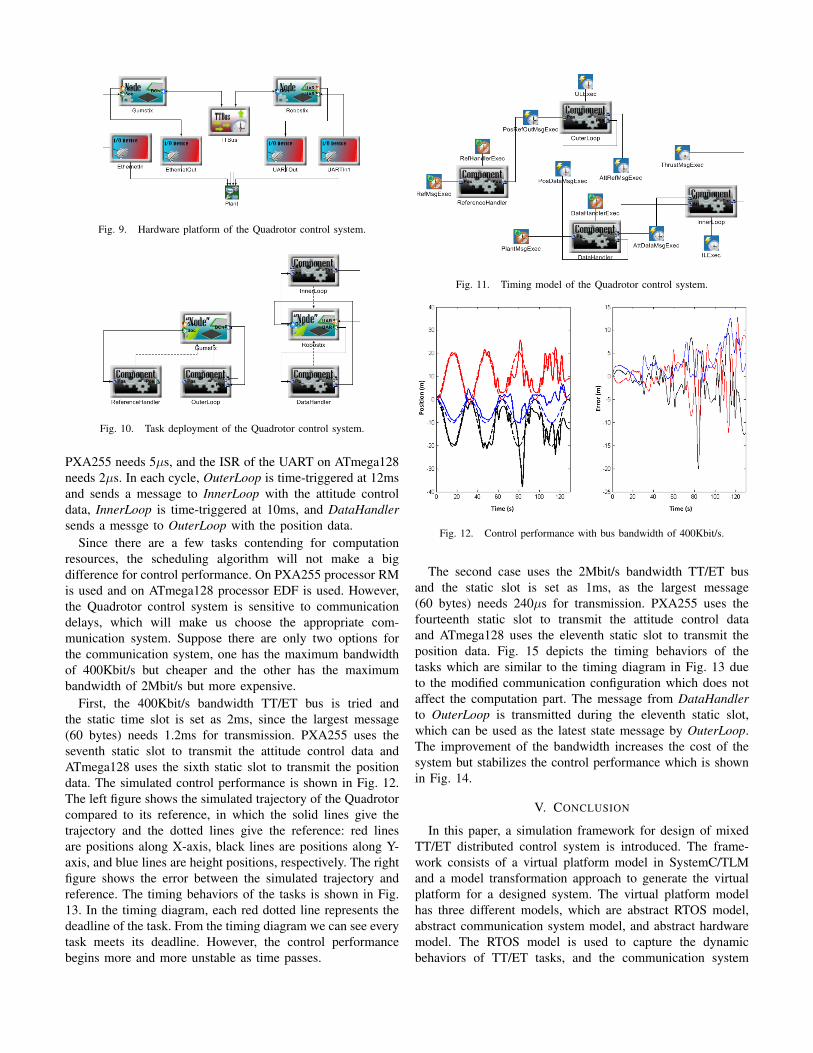
Fig. 9. Hardware platform of the Quadrotor control system.

Fig. 10. Task deployment of the Quadrotor control system.

PXA255 needs 5µs, and the ISR of the UART on ATmega128needs 2µs. In each cycle, OuterLoop is time-triggered at 12msand sends a message to InnerLoop with the attitude controldata, InnerLoop is time-triggered at 10ms, and DataHandlersends a messge to OuterLoop with the position data.

Since there are a few tasks contending for computationresources, the scheduling algorithm will not make a bigdifference for control performance. On PXA255 processor RMis used and on ATmega128 processor EDF is used. However,the Quadrotor control system is sensitive to communicationdelays, which will make us choose the appropriate com-munication system. Suppose there are only two options forthe communication system, one has the maximum bandwidthof 400Kbit/s but cheaper and the other has the maximumbandwidth of 2Mbit/s but more expensive.

First, the 400Kbit/s bandwidth TT/ET bus is tried andthe static time slot is set as 2ms, since the largest message(60 bytes) needs 1.2ms for transmission. PXA255 uses theseventh static slot to transmit the attitude control data andATmega128 uses the sixth static slot to transmit the positiondata. The simulated control performance is shown in Fig. 12.The left figure shows the simulated trajectory of the Quadrotorcompared to its reference, in which the solid lines give thetrajectory and the dotted lines give the reference: red linesare positions along X-axis, black lines are positions along Y-axis, and blue lines are height positions, respectively. The rightfigure shows the error between the simulated trajectory andreference. The timing behaviors of the tasks is shown in Fig.13. In the timing diagram, each red dotted line represents thedeadline of the task. From the timing diagram we can see everytask meets its deadline. However, the control performancebegins more and more unstable as time passes.

Fig. 11. Timing model of the Quadrotor control system.

Fig. 12. Control performance with bus bandwidth of 400Kbit/s.

The second case uses the 2Mbit/s bandwidth TT/ET busand the static slot is set as 1ms, as the largest message(60 bytes) needs 240µs for transmission. PXA255 uses thefourteenth static slot to transmit the attitude control dataand ATmega128 uses the eleventh static slot to transmit theposition data. Fig. 15 depicts the timing behaviors of thetasks which are similar to the timing diagram in Fig. 13 dueto the modified communication configuration which does notaffect the computation part. The message from DataHandlerto OuterLoop is transmitted during the eleventh static slot,which can be used as the latest state message by OuterLoop.The improvement of the bandwidth increases the cost of thesystem but stabilizes the control performance which is shownin Fig. 14.

V. CONCLUSION

In this paper, a simulation framework for design of mixedTT/ET distributed control system is introduced. The frame-work consists of a virtual platform model in SystemC/TLMand a model transformation approach to generate the virtualplatform for a designed system. The virtual platform modelhas three different models, which are abstract RTOS model,abstract communication system model, and abstract hardwaremodel. The RTOS model is used to capture the dynamicbehaviors of TT/ET tasks, and the communication system

Fig. 13. Timing diagram of the control system with bus bandwidth of400Kbit/s.

Fig. 14. Control performance with bus bandwidth of 2Mbit/s.

model is used to capture the behaviors of TT/ET communi-cation. The hardware model integrates the RTOS model andthe communication system model together. Two model trans-formations translate the ESMoL model to the correspondingvirtual platform model for simulation. We present a case studyon a Quadrotor flight control using this framework, and givethe simulation results for different bandwidths of the TT/ETbuses.

The future work includes introducing a more realisticcommunication system model with startup, restart, and clocksynchronization services and more realistic hardware modelsthat give more realistic timing behaviors.

REFERENCES

[1] Byteflight Homepage. http://www.byteflight.com.[2] FlexRay Homepage. http://www.flexray.com.[3] IEEE Standard SystemC Language Reference Manual, 2005.[4] D. D. Gajski, S. Abdi, A. Gerstlauer, and G. Schirner. Embedded System

Design: Modeling, Synthesis and Verification. Springer PublishingCompany, Incorporated, 1st edition, 2009.

[5] A. Gerstlauer, H. Yu, and D. D. Gajski. RTOS Modeling for SystemLevel Design. In Proceedings of the conference on Design, Automationand Test in Europe - Volume 1, DATE ’03, 2003.

[6] Z. He, A. Mok, and C. Peng. Timed RTOS Modeling for EmbeddedSystem Design. In Proceedings of the 11th IEEE Real Time onEmbedded Technology and Applications Symposium, RTAS ’05, pages448–457, 2005.

[7] S. Hong, S. Yoo, S. Lee, S. Lee, H. J. Nam, B.-S. Yoo, J. Hwang,D. Song, J. Kim, J. Kim, H. Jin, K.-M. Choi, J.-T. Kong, and S. Eo.Creation and Utilization of A Virtual Platform for Embedded SoftwareOptimization: An Industrial Case Study. In Proceedings of the 4thinternational conference on Hardware/software codesign and systemsynthesis, CODES+ISSS ’06, pages 235–240, 2006.

[8] Y. Hwang, G. Schirner, S. Abdi, and D. G. Gajski. Accurate TimedRTOS Model for Transaction Level Modeling. In Proceedings of theConference on Design, Automation and Test in Europe, DATE ’10, pages1333–1336, 2010.

Fig. 15. Timing diagram of the system with bus bandwidth of 2Mbit/s.

[9] H. Kopetz and G. Bauer. The Time-Triggered Architecture. Proceedingsof the IEEE, 91(1):112–126, 2003.

[10] N. Kottenstette and J. Porter. Digital Passive Attitude and AltitudeControl Schemes for Quadrotor Aircraft. In Proceedings of the 7thIEEE Intl. Conf. on Control and Automation, ICCA ’09, ChristChurch,New Zealand, 2009.

[11] R. Le Moigne, O. Pasquier, and J.-P. Calvez. A Generic RTOS Modelfor Real-time Systems Simulation with SystemC. In Proceedings of theconference on Design, automation and test in Europe - Volume 3, DATE’04, pages 30082–, 2004.

[12] A. Ledeczi, M. Maroti, A. Bakay, G. Karsai, J. Garrett, C. Thomason,G. Nordstrom, J. Sprinkle, and P. Volgyesi. The generic modelingenvironment. In Workshop on Intelligent Signal Processing, 2001.

[13] A. Metzner. Analyzing Mixed Event Triggered/Time Triggered Systems.[14] K. D. Nguyen, P. S. Thiagarajan, and W.-F. Wong. A UML-Based

Design Framework for Time-Triggered Applications. In Proceedings ofthe 28th IEEE International Real-Time Systems Symposium, RTSS ’07,pages 39–48, 2007.

[15] S. Park, W. Olds, K. G. Shin, and S. Wang. Integrating Virtual ExecutionPlatform for Accurate Analysis in Distributed Real-Time Control SystemDevelopment. In Proceedings of the 28th IEEE International Real-TimeSystems Symposium, RTSS ’07, pages 61–72, 2007.

[16] J. Perez, A. Perez, and R. Obermaisser. Executable Time-Triggered Model (E-TTM) for Real-Time Control Systems. InProceedings of the 2010 13th IEEE International Symposium onObject/Component/Service-Oriented Real-Time Distributed Computing,ISORC ’10, pages 42–49, 2010.

[17] T. Pop, P. Eles, and Z. Peng. Design Optimization of Mixed Time/Event-Triggered Distributed Embedded Systems. In Proceedings of the 1stIEEE/ACM/IFIP international conference on Hardware/software code-sign and system synthesis, CODES+ISSS ’03, pages 83–89, 2003.

[18] T. Pop, P. Eles, and Z. Peng. Schedulability Analysis for DistributedHeterogeneous Time/Event Triggered Real-Time Systems. In Proceed-ings of the 15th EuroMicro Conf. on Real-Time Systems, ECRTS ’03,pages 257–266, 2003.

[19] J. Porter and G. Hemingway et al. The ESMoL Language andTools for High-Confidence Distributed Control Systems Design. Part1: Language, Framework, and Analysis. Technical Report ISIS-10-109,ISIS, Vanderbilt Univ., 2010.

[20] J. M. Rushby. Bus Architectures for Safety-Critical Embedded Systems.In Proceedings of the First International Workshop on EmbeddedSoftware, EMSOFT ’01, pages 306–323, 2001.

[21] N. Scaife and P. Caspi. Integrating Model-Based Design and PreemptiveScheduling in Mixed Time- and Event-Triggered Systems. In Proceed-ings of the 16th Euromicro Conference on Real-Time Systems, ECRTS’04, pages 119–126, 2004.

[22] J. Sztipanovits, X. D. Koutsoukos, G. Karsai, N. Kottenstette, P. J.Antsaklis, V. Gupta, B. Goodwine, J. S. Baras, and S. Wang. Toward ascience of cyber-physical system integration. Proceedings of the IEEE,100(1):29–44, 2012.

[23] T. Yokoyama. An Aspect-Oriented Development Method for EmbeddedControl Systems with Time-Triggered and Event-Triggered Processing.In Proceedings of the 11th IEEE Real Time on Embedded Technologyand Applications Symposium, RTAS ’05, pages 302–311, 2005.

[24] H. Zabel, W. Muller, and A. Gerstlauer. Accurate RTOS Modeling andAnalysis with SystemC. In W. Ecker, W. Muller, and R. Domer, editors,Hardware-dependent Software, chapter 9, pages 233–260. SpringerNetherlands, 2009.

An Analytical Model of the CAN Bus for Online Schedulability Test

Zhenwu Shi and Fumin Zhang, Georgia Institute of Technology

Abstract—Controller area network (CAN) is a priority-based bus that supports real-time communication. Existingschedulability analysis for the CAN bus is peformed at thedesign stage, by assuming that all message information isknown in advance. However, in pratice, the CAN bus mayrun in a dynamic environment, where complete specificationsmay not be available at the design stage and operationalrequirements may change at system run-time. In this paper,we develop an analytical model that describes the dynamics ofmessage transmission on the CAN bus. Based on this analyticaltiming model, we then propose an online test that effectivelychecks the schedulability of the CAN bus, in the presence ofonline adjustments of message streams. Simulations show thatthe online test can accurately report the loss of scheduabilityon the CAN bus.

I. INTRODUCTION

Controller area network (CAN bus) is a serial bus de-signed for industrial environments. It was first deployed bythe automobile industry in the 1980s for decreasing wiringhardness and complexity among electronic control units invehicles. During the past thirty years, other industries havegradually adopted the CAN bus and applied it to a varietyof areas such as robotics, aircraft, medical equipment, andindustrial automation. The CAN bus has an important featureof supporting real-time communication. Each message onthe CAN bus is assigned a priority and the transmissionof messages follows a deterministic order decided by theirprorities [1]. This feature makes the CAN bus particularlysuitable for systems with stringent time constraints on thecommunication.

Related Works The application of the CAN bus requiresscheduling analysis to check if all messages can meet theirdeadlines. The scheduling analysis of the CAN bus hasbeen extensively studied. In 1994, Tindell et al. proposeda basic CAN schedulability analysis [2]–[4]. This result waslater recognized by Volvo Car Corporation and successfullyused as the theoretical foundation for commercial CANschedulability analysis tools [5]. However, the basic CANschedulability analysis in [2]–[4] is based on ideal assump-tions of the CAN bus that may not be supported in realapplications. Since then, a lot of research has been conductedto improve the basic CAN schedulability analysis. [6]–[9]

The research is supported by ONR grants N00014-08-1-1007, N00014-09-1-1074, and N00014-10-10712 (YIP), and NSF grants ECCS-0841195(CAREER), CNS-0931576, and ECCS-1056253.

Zhenwu Shi and Fumin Zhang are with the School of Electrical andComputer Engineering, Georgia Institute of Technology, Atlanta, GA,30332, USA zwshi, [email protected]

studied the effect of hardware limitations on the schedulinganalysis of the CAN bus. [10]–[12] extended the basic CANschedulability analysis to account for the transmission errors.[13], [14] studied the schedulability issues of the CAN buswhen messages have offsets. [15] proposed a probalisticanalysis of the response time of messages on the CAN bus.In 2007, Davis et al. revisted the basic CAN schedulabilityanalysis and corrected some significant flaws [16].

Motivation. Existing schedulability analysis for the CANbus is performed at the design stage, by assuming that all ofmessage information is known in advance. This assumptionused to be valid in the earlier design of embedded systems,which deliberately abstracted away properties of the physicalworld. However, this is not always be the case. Recent yearshave witnessed a growing trend for developing embeddedsystems that are closely integrated with the physical world.For example, Cyber Physical Systems research communityhas emerged, with the aim of underpinning the integrationof cyber and physical elements across all application sectors[17], [18]. However, one of the major design challengesbrought by this trend is that the embedded system needsto operate in a dynamic environment, where completespecifications are not possible at the design stage and/oroperational requirements may change at system runtime[19]. Particularly concerning the CAN bus in embeddedsystems, the design challenge means that the CAN bus mayfrequently experience online adjustment of communicationrequirements, such as addition, removal, and change ofmessage streams. To guarantee normal operation of the CANbus in a dynamic environment, we need an online test thatcan check the schedulability of the CAN bus during systemruntime.

Contributation. In this paper, we analytically model thedynamics of message transmission on the CAN bus througha non-block, deterministic hybrid automaton. Then, basedon this analytical timing model, we propose an online testthat re-evaluates the schedulability of the CAN bus. Ourcontribution is two manifold: (1) an analytical model of theCAN bus; and (2) an online schedulability test, which isnecessary and sufficient, hence gives the least conservativeschedulability test.

Organization. The remainder of this paper is organizedas follows. Section II presents an overview of the CANprotocol. Section III formulates the problem. Section IV usesa hybrid automaton to analytically describe the dynamics ofscheduling messages on the CAN bus. Section V proposed

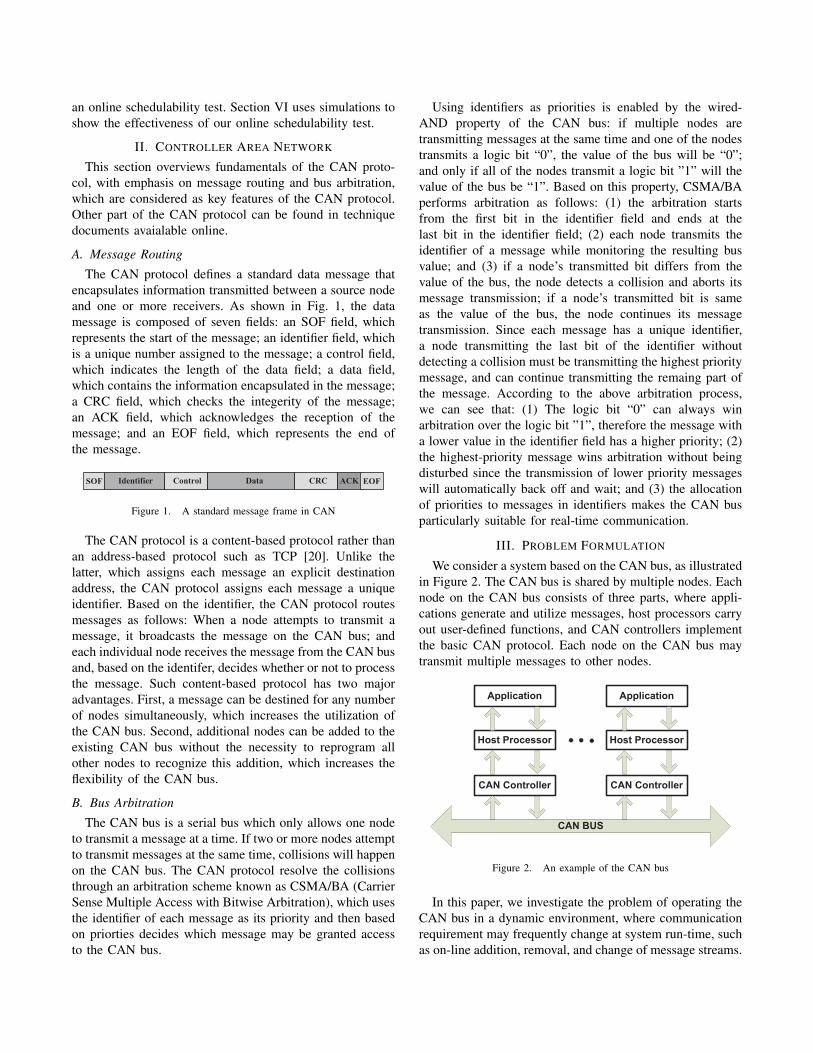
an online schedulability test. Section VI uses simulations toshow the effectiveness of our online schedulability test.

II. CONTROLLER AREA NETWORK

This section overviews fundamentals of the CAN proto-col, with emphasis on message routing and bus arbitration,which are considered as key features of the CAN protocol.Other part of the CAN protocol can be found in techniquedocuments avaialable online.

A. Message Routing

The CAN protocol defines a standard data message thatencapsulates information transmitted between a source nodeand one or more receivers. As shown in Fig. 1, the datamessage is composed of seven fields: an SOF field, whichrepresents the start of the message; an identifier field, whichis a unique number assigned to the message; a control field,which indicates the length of the data field; a data field,which contains the information encapsulated in the message;a CRC field, which checks the integerity of the message;an ACK field, which acknowledges the reception of themessage; and an EOF field, which represents the end ofthe message.

SOF Identifier Control . CRC ACK EOFCONTROLData

Figure 1. A standard message frame in CAN

The CAN protocol is a content-based protocol rather thanan address-based protocol such as TCP [20]. Unlike thelatter, which assigns each message an explicit destinationaddress, the CAN protocol assigns each message a uniqueidentifier. Based on the identifier, the CAN protocol routesmessages as follows: When a node attempts to transmit amessage, it broadcasts the message on the CAN bus; andeach individual node receives the message from the CAN busand, based on the identifer, decides whether or not to processthe message. Such content-based protocol has two majoradvantages. First, a message can be destined for any numberof nodes simultaneously, which increases the utilization ofthe CAN bus. Second, additional nodes can be added to theexisting CAN bus without the necessity to reprogram allother nodes to recognize this addition, which increases theflexibility of the CAN bus.

B. Bus Arbitration

The CAN bus is a serial bus which only allows one nodeto transmit a message at a time. If two or more nodes attemptto transmit messages at the same time, collisions will happenon the CAN bus. The CAN protocol resolve the collisionsthrough an arbitration scheme known as CSMA/BA (CarrierSense Multiple Access with Bitwise Arbitration), which usesthe identifier of each message as its priority and then basedon priorties decides which message may be granted accessto the CAN bus.

Using identifiers as priorities is enabled by the wired-AND property of the CAN bus: if multiple nodes aretransmitting messages at the same time and one of the nodestransmits a logic bit “0”, the value of the bus will be “0”;and only if all of the nodes transmit a logic bit ”1” will thevalue of the bus be “1”. Based on this property, CSMA/BAperforms arbitration as follows: (1) the arbitration startsfrom the first bit in the identifier field and ends at thelast bit in the identifier field; (2) each node transmits theidentifier of a message while monitoring the resulting busvalue; and (3) if a node’s transmitted bit differs from thevalue of the bus, the node detects a collision and aborts itsmessage transmission; if a node’s transmitted bit is sameas the value of the bus, the node continues its messagetransmission. Since each message has a unique identifier,a node transmitting the last bit of the identifier withoutdetecting a collision must be transmitting the highest prioritymessage, and can continue transmitting the remaing part ofthe message. According to the above arbitration process,we can see that: (1) The logic bit “0” can always winarbitration over the logic bit ”1”, therefore the message witha lower value in the identifier field has a higher priority; (2)the highest-priority message wins arbitration without beingdisturbed since the transmission of lower priority messageswill automatically back off and wait; and (3) the allocationof priorities to messages in identifiers makes the CAN busparticularly suitable for real-time communication.

III. PROBLEM FORMULATION

We consider a system based on the CAN bus, as illustratedin Figure 2. The CAN bus is shared by multiple nodes. Eachnode on the CAN bus consists of three parts, where appli-cations generate and utilize messages, host processors carryout user-defined functions, and CAN controllers implementthe basic CAN protocol. Each node on the CAN bus maytransmit multiple messages to other nodes.

CAN BUS

CAN Controller

Host Processor

Application

CAN Controller

Host Processor

Application

Figure 2. An example of the CAN bus

In this paper, we investigate the problem of operating theCAN bus in a dynamic environment, where communicationrequirement may frequently change at system run-time, suchas on-line addition, removal, and change of message streams.

The online adjustment of message streams may lead to theunschedulability of the CAN bus. Thus, it is necessary tointroduce a new way to re-evaluate the schedulability of theCAN bus at system run-time as follows:

Definition 3.1: An online schedulability test over a timeinterval [ta, tb] checks if all message instances are able tomeet their deadlines within [ta, tb].As the starting time increases, the time interval [ta, tb] willslide forward. The length of the interval tb − ta dependson how much into the future we want to perform theschedulability test. All mathematical tools developed in thispaper are centered around the online schedulability testwithin the time interval [ta, tb].

A. System Configuration

There are many different ways of desigining the architec-ture of the CAN bus. Each design may lead to a differentmodel. In this paper, we assume that the CAN bus in Figure2 satisfies the following conditions

1) The CAN bus is reliable such that no error exists inthe transmission;

2) At each node, among all messages that are ready fortransmission, the message with the highest prioritywill be always transmitted first.

The above conditions are conventional assumptions that havebeen widely used in the research community of the CANbus. As a first step towards the analytical modeling of theCAN bus, we rely on them for our derivation. While theabove conditions may not be satisfied in all applicationscenarios, we believe that refined modeling can be carriedout under the same framework .

Moreover, we configure the CAN bus such that eachnode will automatically drop off transmission requests ofmessages that cannot meet their deadlines.

B. Model and Notations

We describe a system model for the CAN bus and severalnotations that will be used in the rest of the paper.

Consider a set of independent messages {τ1, · · · , τN}transmitting on the CAN bus within the time interval[ta, tb]. Each message τn is characterized by a tuple{akn, Ck

n, Tkn , E

kn, P

kn} defined as follows:

• akn: the release time of the the k -th instance of τn;• Ck

n: the transmission time of the k -th instance of τn;• T k

n : the inter-release time, i.e. T kn = ak+1

n − akn;• Ek

n: the relative deadline of the k -th instance of τn;• P k

n : the identifier of the k -th instance of τn;Note that the characteristics of τn is defined at the instancelevel. Such definition allows each instance of τn to have dif-ferent characteristics, which makes our model applicable tonot only periodic messages but also non-periodic messages.

Remark 3.2: Since the CAN bus operates in a environ-ment where the communication requirement may frequentlychange, the set of messages {τ1, · · · , τN} may dynamicallyadjust at runtime.

IV. AN ANALYTICAL TIMING MODEL FOR SCHEDULINGON THE CAN BUS

In last section, we have established necessary notations todescribe a set of messages on the CAN bus. In this section,we will develop an analytical timing model that describesthe dynamics of scheduling messages on the CAN bus.

A. State Variables

To describe how message {τ1, · · · , τN} are scheduled onthe CAN bus from a dynamic system point of view, weintroduce a state vector Z(t) = [D(t), R(t), O(t)].

Definition 4.1: The first component D(t) is defined as avector D(t) = [d1(t), · · · , dN (t)], where dn(t), for n =1, 2, · · · , N , denotes how long after t the next instance ofτn will be released.

Definition 4.2: The second component R(t) is defined asa vector R(t) = [r1(t), ..., rN (t)], where rn(t), for n =1, 2, ..., N , denotes the remaining transmission time of thecurrent instance of τn after time t.

Definition 4.3: The third component O(t) is defined asa vector O(t) = [o1(t), ..., oN (t)], where on(t), for n =1, 2, ..., N , denotes how much time has elapsed before thecurrent instance of τn finishes transmission.

With the state vector well defined, we can study thedynamics of scheduling {τ1, · · · , τN} on the CAN busthrough the evolution of Z(t).

B. Evolution of State Vector

The state vector Z(t) evolve continuously most of thetime, except when two “special” events happen. One specialevent is the arrival of a new instance. When this eventhappens, the value of Z(t) is reset to the characteristics ofthe new instance. The other special event is that a messagefinishes transmission on the CAN bus and another messagestarts transmission. When this event happens, the evolutiondynamics of Z(t) switches discontinuously. Since the statevector Z(t) exhibits both continuous and discrete dynamicbehaviors, the evolution of Z(t) can be described by a hybridautomaton defined as follows.

Definition 4.4: A hybrid automaton that describes thedynamics of scheduling {τ1, · · · , τN} is a collection H ={Q,Z, F,Dom,Edge,Guard,Reset} where

• Q = {q0, q1, · · · , qN} is a set of modes, where themode q0 indicates that no message is being transmittedon the CAN bus and the mode qi (1 ≤ i ≤ N ) indicatesthat τi is being transmitted on the CAN bus;

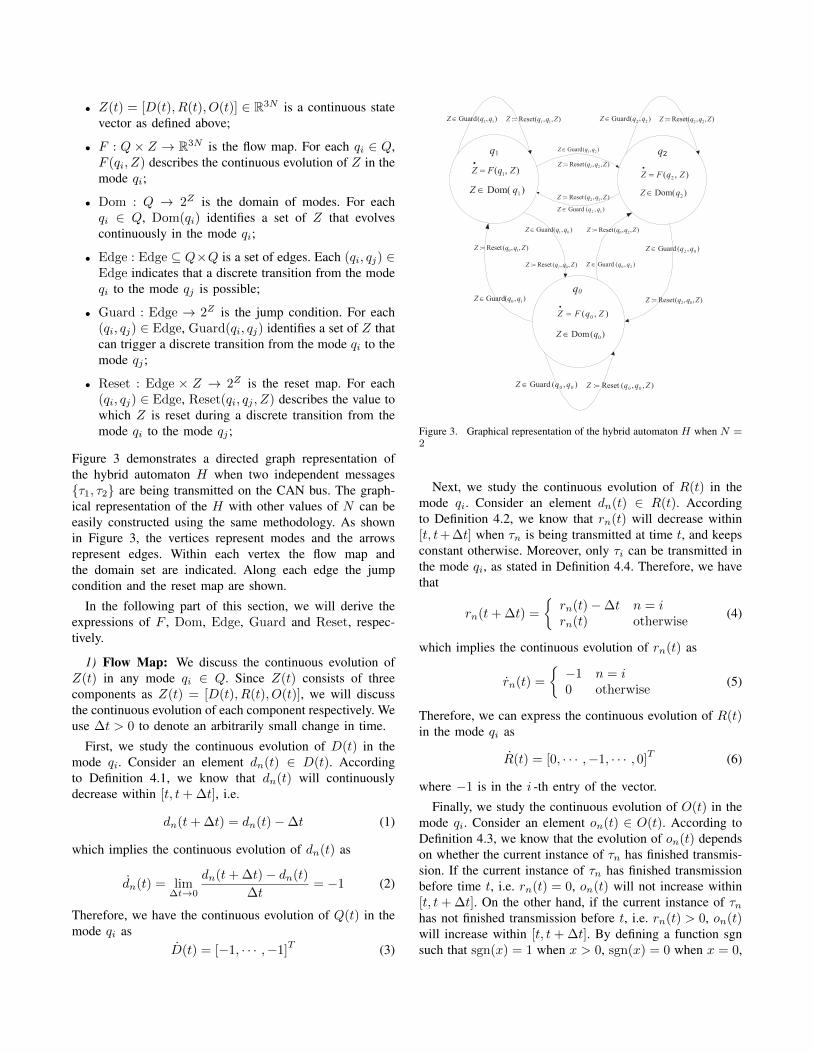
• Z(t) = [D(t), R(t), O(t)] ∈ R3N is a continuous statevector as defined above;

• F : Q× Z → R3N is the flow map. For each qi ∈ Q,F (qi, Z) describes the continuous evolution of Z in themode qi;

• Dom : Q → 2Z is the domain of modes. For eachqi ∈ Q, Dom(qi) identifies a set of Z that evolvescontinuously in the mode qi;

• Edge : Edge ⊆ Q×Q is a set of edges. Each (qi, qj) ∈Edge indicates that a discrete transition from the modeqi to the mode qj is possible;

• Guard : Edge → 2Z is the jump condition. For each(qi, qj) ∈ Edge, Guard(qi, qj) identifies a set of Z thatcan trigger a discrete transition from the mode qi to themode qj ;

• Reset : Edge × Z → 2Z is the reset map. For each(qi, qj) ∈ Edge, Reset(qi, qj , Z) describes the value towhich Z is reset during a discrete transition from themode qi to the mode qj ;

Figure 3 demonstrates a directed graph representation ofthe hybrid automaton H when two independent messages{τ1, τ2} are being transmitted on the CAN bus. The graph-ical representation of the H with other values of N can beeasily constructed using the same methodology. As shownin Figure 3, the vertices represent modes and the arrowsrepresent edges. Within each vertex the flow map andthe domain set are indicated. Along each edge the jumpcondition and the reset map are shown.

In the following part of this section, we will derive theexpressions of F , Dom, Edge, Guard and Reset, respec-tively.

1) Flow Map: We discuss the continuous evolution ofZ(t) in any mode qi ∈ Q. Since Z(t) consists of threecomponents as Z(t) = [D(t), R(t), O(t)], we will discussthe continuous evolution of each component respectively. Weuse ∆t > 0 to denote an arbitrarily small change in time.

First, we study the continuous evolution of D(t) in themode qi. Consider an element dn(t) ∈ D(t). Accordingto Definition 4.1, we know that dn(t) will continuouslydecrease within [t, t+ ∆t], i.e.

dn(t+ ∆t) = dn(t)−∆t (1)

which implies the continuous evolution of dn(t) as

dn(t) = lim∆t→0

dn(t+ ∆t)− dn(t)

∆t= −1 (2)

Therefore, we have the continuous evolution of Q(t) in themode qi as

D(t) = [−1, · · · ,−1]T (3)

q0

),( 0 ZqFZ =

·

),( 1 ZqFZ =·

)Dom( 1qZ Î

q1 q2

),(Guard 11 qqZ Î ),,(Reset: 1 ZqqZ 1=

)(Dom 0qZ Î

),( 2 ZqFZ =·

)Dom( 2qZ Î

),(Guard 22 qqZ Î ),,(Reset: 22 ZqqZ =

),(Guard 21 qqZ Î

),,(Reset: 2 ZqqZ 1=

),(Guard 12 qqZ Î

),,(Reset: 12 ZqqZ =

),(Guard 01 qqZ Î

),,(Reset: 0 ZqqZ 1=

),(Guard 10 qqZÎ


),(Guard 20 qqZ Î


),(Guard 02 qqZ Î


),(Guard 00 qqZ Î ),,(Reset: 00 ZqqZ =

Figure 3. Graphical representation of the hybrid automaton H when N =2

Next, we study the continuous evolution of R(t) in themode qi. Consider an element dn(t) ∈ R(t). Accordingto Definition 4.2, we know that rn(t) will decrease within[t, t+ ∆t] when τn is being transmitted at time t, and keepsconstant otherwise. Moreover, only τi can be transmitted inthe mode qi, as stated in Definition 4.4. Therefore, we havethat

rn(t+ ∆t) =

{rn(t)−∆t n = irn(t) otherwise

(4)

which implies the continuous evolution of rn(t) as

rn(t) =

{−1 n = i0 otherwise

(5)

Therefore, we can express the continuous evolution of R(t)in the mode qi as

R(t) = [0, · · · ,−1, · · · , 0]T (6)

where −1 is in the i -th entry of the vector.

Finally, we study the continuous evolution of O(t) in themode qi. Consider an element on(t) ∈ O(t). According toDefinition 4.3, we know that the evolution of on(t) dependson whether the current instance of τn has finished transmis-sion. If the current instance of τn has finished transmissionbefore time t, i.e. rn(t) = 0, on(t) will not increase within[t, t+ ∆t]. On the other hand, if the current instance of τnhas not finished transmission before t, i.e. rn(t) > 0, on(t)will increase within [t, t + ∆t]. By defining a function sgnsuch that sgn(x) = 1 when x > 0, sgn(x) = 0 when x = 0,

and sgn(x) = 1 when x < 0, we have that

on(t+ ∆t) = on(t) + sgn(rn(t)) ∆t (7)

which implies the continuous evolution of on(t) as

on(t) = lim∆t→0

on(t+ ∆t)− on(t)

∆t= sgn(rn(t)) (8)

Therefore, we have the continuous evolution of O(t) in themode qi as

O(t) = [sgn(r1(t)), · · · , sgn(rN (t))]T (9)

In summary, equation (3), (6) and (9) constitute the contin-uous evolution of Z(t) in any mode qi ∈ Q.

2) Domain of Modes: For the ease of expression, wedefine an auxiliary variable G(t) as follows

Definition 4.5: G(t) is a set of indices of messages, whichare active for transmission at time t.

G(t) ={n| rn(t) = Ck

n and on(t) + Ckn ≤ Ek

n

}(10)

where k represents the index of the current instance of τnat time t, rn(t) = Ck

n specifies messages that have nottransmitted yet, and on(t) + Ck

n < Ekn specifies messages

that can meet their deadlines.In the mode q0, the state Z will continuously evolve as

long as the following two conditions are both satisfied: nonew instance of {τ1, · · · , τN} is released and no message isactive for transmission on the CAN bus. To meet the firstcondition, we have that

min1≤n≤N

{D(t)} > 0 (11)

where Definition 4.1 is applied. To meet the second condi-tion, we have that

Card (G(t)) = 0 (12)

where Card(·) is a cardinality function that measures thenumber of elements in a set. Therefore, we have the domainof the mode q0 as

Dom(q0)=

{Z(t) | min

1≤n≤N{D(t)}>0 and Card(G(t))=0

}(13)

In any other mode qi where 1 ≤ i ≤ N , the state Z willcontinuously evolve as long as the following two conditionsare both satisfied: no new instance of {τ1, · · · , τN} isreleased and τi is being transmitted on the CAN bus. Tomeet the first condition, we have that

min1≤n≤N

{D(t)} > 0 (14)

where Definition 4.1 is applied. To meet the second condi-tion, we have that

0 < ri(t) ≤ Cki (15)

Therefore, we have the domain of the mode qi where 1 ≤i ≤ N as

Dom(qi)=

{Z(t)| min

1≤n≤N{D(t)} > 0 and 0 < ri(t) ≤ Ck

i

}(16)

3) Edges and Jump Conditions: According to thedefinition of Q, we know that the transition between anytwo modes is possible. Therefore, we have that

Edge = Q×Q (17)

where an edge (qi, qj) ∈ Edge represents a transition fromthe mode qi to the mode qj .

For any edge (qi, qj) ∈ Edge, we discuss the jumpcondition Guard(qi, qj). Our discussion on jump conditionscan be classified into four cases according to different edges.

Case 1: an edge where i = j. This transition is triggeredwhen any message in {τ1, · · · , τN} release a new instance,i.e.

Guard(qi, qi) = { min1≤n≤N

{D(t)} = 0} (18)

Case 2: an edge where i 6= j and 1 ≤ i, j ≤ N . Thistransition is triggered when τi finishes transmission and τjstarts transmission. Thus, we have

Guard(qi, qj) = {ri(t) = 0 and j = argminn∈G(t)

P kn} (19)

where ri(t) = 0 indicates that τi has finished transmissionon the CAN bus at time t and j = argminn∈G(t)P

kn

indicates that τj has the highest priority among all messagesthat are active for transmission at time t.

Case 3: an edge where 1 ≤ i ≤ N and j = 0. This transitionis triggered when τi finishes transmission and no messageis active for transmission at time t. Thus, we have

Guard(qi, q0) = {ri(t) = 0 and Card (G(t)) = 0} (20)

where ri(t) = 0 indicates that τi has finished transmissionat time t and Card (G(t)) = 0 indicates that no message isactive for transmission at time t.

Case 4: an edge where i = 0 and 1 ≤ j ≤ N . This transitionis triggered when τi starts its transmission after the CAN bushas been idle for a while.

Guard(q0, qj) = {Card (G(t)) > 0 and j = argminn∈G(t)

P kn}

(21)where Card (G(t)) > 0 indicates that there are messagesactive for transmission on the CAN bus at time t and j =argminn∈G(t)P

kn indicates that τj has the highest priority

among all messages that are active for transmission at timet.

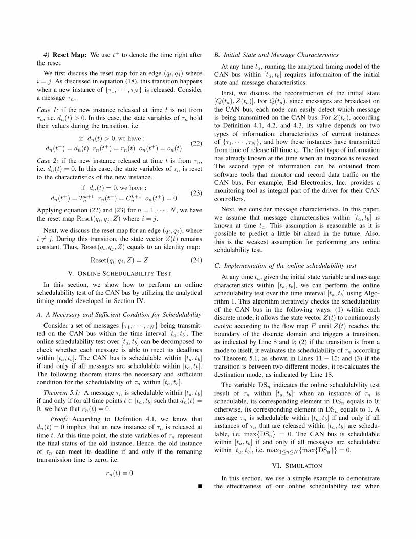
4) Reset Map: We use t+ to denote the time right afterthe reset.

We first discuss the reset map for an edge (qi, qj) wherei = j. As discussed in equation (18), this transition happenswhen a new instance of {τ1, · · · , τN} is released. Considera message τn.

Case 1: if the new instance released at time t is not fromτn, i.e. dn(t) > 0. In this case, the state variables of τn holdtheir values during the transition, i.e.

if dn(t) > 0,we have :

dn(t+) = dn(t) rn(t+) = rn(t) on(t+) = on(t)(22)

Case 2: if the new instance released at time t is from τn,i.e. dn(t) = 0. In this case, the state variables of τn is resetto the characteristics of the new instance.

if dn(t) = 0,we have :

dn(t+) = T k+1n rn(t+) = Ck+1

n on(t+) = 0(23)

Applying equation (22) and (23) for n = 1, · · · , N , we havethe reset map Reset(qi, qj , Z) where i = j.

Next, we discuss the reset map for an edge (qi, qj), wherei 6= j. During this transition, the state vector Z(t) remainsconstant. Thus, Reset(qi, qj , Z) equals to an identity map:

Reset(qi, qj , Z) = Z (24)

V. ONLINE SCHEDULABILITY TEST

In this section, we show how to perform an onlineschedulability test of the CAN bus by utilizing the analyticaltiming model developed in Section IV.

A. A Necessary and Sufficient Condition for Schedulability

Consider a set of messages {τ1, · · · , τN} being transmit-ted on the CAN bus within the time interval [ta, tb]. Theonline schedulability test over [ta, tb] can be decomposed tocheck whether each message is able to meet its deadlineswithin [ta, tb]. The CAN bus is schedulable within [ta, tb]if and only if all messages are schedulable within [ta, tb].The following theorem states the necessary and sufficientcondition for the schedulability of τn within [ta, tb].

Theorem 5.1: A message τn is schedulable within [ta, tb]if and only if for all time points t ∈ [ta, tb] such that dn(t) =0, we have that rn(t) = 0.

Proof: According to Definition 4.1, we know thatdn(t) = 0 implies that an new instance of τn is released attime t. At this time point, the state variables of τn representthe final status of the old instance. Hence, the old instanceof τn can meet its deadline if and only if the remaningtransmission time is zero, i.e.

rn(t) = 0

B. Initial State and Message Characteristics

At any time ta, running the analytical timing model of theCAN bus within [ta, tb] requires informaiton of the initialstate and message characteristics.

First, we discuss the reconstruction of the initial state[Q(ta), Z(ta)]. For Q(ta), since messages are broadcast onthe CAN bus, each node can easily detect which messageis being transmitted on the CAN bus. For Z(ta), accordingto Definition 4.1, 4.2, and 4.3, its value depends on twotypes of information: characteristics of current instancesof {τ1, · · · , τN}, and how these instances have transmittedfrom time of release till time ta. The first type of informationhas already known at the time when an instance is released.The second type of information can be obtained fromsoftware tools that monitor and record data traffic on theCAN bus. For example, Esd Electronics, Inc. provides amonitoring tool as integral part of the driver for their CANcontrollers.

Next, we consider message characteristics. In this paper,we assume that message characteristics within [ta, tb] isknown at time ta. This assumption is reasonable as it ispossible to predict a little bit ahead in the future. Also,this is the weakest assumption for performing any onlineschdulability test.

C. Implementation of the online schedulability test

At any time ta, given the initial state variable and messagecharacteristics within [ta, tb], we can perform the onlineschedulability test over the time interval [ta, tb] using Algo-rithm 1. This algorithm iteratively checks the schedulabilityof the CAN bus in the following ways: (1) within eachdiscrete mode, it allows the state vector Z(t) to continuouslyevolve according to the flow map F until Z(t) reaches theboundary of the discrete domain and triggers a transition,as indicated by Line 8 and 9; (2) if the transition is from amode to itself, it evaluates the schedulability of τn accordingto Theorem 5.1, as shown in Lines 11 − 15; and (3) if thetransition is between two different modes, it re-calcuates thedestination mode, as indicated by Line 18.

The variable DSn indicates the online schedulability testresult of τn within [ta, tb]: when an instance of τn isschedulable, its corresponding element in DSn equals to 0;otherwise, its corresponding element in DSn equals to 1. Amessage τn is schedulable within [ta, tb] if and only if allinstances of τn that are released within [ta, tb] are schedu-lable, i.e. max{DSn} = 0. The CAN bus is schedulablewithin [ta, tb] if and only if all messages are schedulablewithin [ta, tb], i.e. max1≤n≤N{max{DSn}} = 0.

VI. SIMULATION

In this section, we use a simple example to demonstratethe effectiveness of our online schedulability test when

Algorithm 1: Online Schedulability Test/*Schedulability of the CAN bus within [ta, tb] */Data: ta, tb, Q(t−a ), Z(t−a ), {Ck

n, Tkn , E

kn, P

kn}Nn=1

Result: {DSn}Nn=1

1 t = ta; mode = Q(t−a );2 for n = 1 to N do3 DSn = [ ];

4 while t < tb do5 switch mode do6 · · · · · · ;7 case n :8 while Z(t) ∈ Dom(qn) do9 Z(t) = F (qn, Z(t));

10 if min1≤n≤N

{D(t)} == 0 then

11 for n = 1 to N do12 if dn(t) == 0 and rn(t) == 0 then13 DSn = [DSn 0];

14 else if dn(t) == 0 and rn(t) > 0then

15 DSn = [DSn 1];

16 Z(t) = Reset(qn, qn, Z(t));

17 else18 Re-calculate the value of mode ;

19 · · · · · · ;

20 return {DSn}Nn=1;

message streams on the CAN bus frequently changes. Ourmethods can be easily applied to more complex examples.

At the design stage, we assume that three periodic mes-sages {τ1, τ2, τ3} start their transmission on the CAN bussimultaneously from time 0. The three messages have thefollowing characteristics[

T k1 , T

k2 , T

k3

]= [ 200, 250, 300 ] ms,[

Ck1 , C

k2 , C

k3

]= [ 40 , 50 , 60 ] ms,[

Ek1 , E

k2 , E

k3

]= [ 100, 175, 200 ] ms.

Moreover, the three messages are assigned unique identifierssuch that

P k1 < P k

2 < P k3

which implies that τ1 has a higher priority than τ2, whichhas a higher priority than τ3.

At system run-time, we consider two types of onlinecommunication adjustments. One is the change of messageperiods. We assume that τ1 and τ2 change their periodswithin [22, 26]s as[

T k1 , T

k2

]= [160, 210] ms.

The other type of online adjustment is the addition of newmessages. We assume that another periodic messages τ4appears on the CAN bus within [20, 26]s. The new messagehas the following characteristics[

T k4 , C

k4 , E

k4

]= [ 200, 50, 200] ms,

Moreover, the new message is assigned a unique identifiersuch that

P k1 < P k

4 < P k2 < P k

3

Figure 4(a) shows the transmission of four messages onthe CAN bus within the time interval [20.5, 23.5]s. Thevalue ”0.5” indicates that the transmission of the message isblocked by other higher priority messages on the CAN bus;the value ”1” indicates that the message is being transmittedon the CAN bus; and the value ”0” indicates that the messagefinishes transmission. By closely examining Figure 4(a),we can see that two instances of τ3 that are released attime 21s and time 22.8s have not been transmitted beforetheir deadlines. Figure 4(a) shows the online schedulabilitytest of the CAN bus within the time interval [20.5, 23.5].As discussed in Section V, the value ”1” indicates thatan instance fails to meet its deadline and the value ”0”indicates that an instance meets its deadline. According toFigure 4(b), we can easily see that two instances of τ3 thatare released at time 21s and time 22.8s fail to meet theirdeadlines. Therefore, the observation in Figure 4(b) exactlymatch that in Figure 4(a), which implies that our onlineschedulability test can accurately identify the unschedulablemessage instances.

VII. CONCLUSION

This paper proposes an online schedulability test of theCAN bus, which is based on an analytical model. Thesimulations show that the online schedulability test canaccurately report the lost of schedulability on the CAN bus.

REFERENCES

[1] R. B. Gmbh, “CAN Specification Version 2.0,” Stuttgart,Germany, Tech. Rep., 1991.

[2] K. W. Tindell, H. Hansson, and A. J. Wellings, “Analysingreal-time communications: controller area network (CAN),” inProc. of IEEE International Conference on Real-Time SystemsSymposium, Dec. 1994, pp. 259–263.

[3] K. Tindell and A. Burns, “Guarantee Message Latency onControl Area Network(CAN),” in Proc. of International CANConference, 1994, pp. 1–11.

[4] K. Tindell, A. Burns, and A. Wellings, “Calculating Con-troller Area Network (CAN) message response times,” Con-trol Engineering Practice, vol. 3, no. 8, pp. 1163–1169, 1995.

[5] L. Casparsson, A. Rajnak, K. Tindell, and P. Malmberg,“Volcano-a revolution in on-board communications,” VolvoTechnology Report, Tech. Rep., 1998.

20.5 21 21.5 22 22.5 23

0

1

Transmission of the First Message

20.5 21 21.5 22 22.5 23

0

1

Transmission of the Second Message

20.5 21 21.5 22 22.5 23

0

1

Transmission of the Third Message

20.5 21 21.5 22 22.5 23

0

1

Transmission of the Fourth Message

(a) Transmission of Messages

20.5 21 21.5 22 22.5 23

0

1

Schedulability of the First Message

20.5 21 21.5 22 22.5 23

0

1

Schedulability of the Second Message

20.5 21 21.5 22 22.5 23

0

1

Schedulability of the Third Message

20.5 21 21.5 22 22.5 23

0

1

Schedulability of the Fourth Message

(b) Online Schedulability Test Result

Figure 4. The dynamics of the CAN bus within [20.523.3]s

[6] M. D. Natale, “Evaluating message transmission times inController Area Networks without buffer preemption,” inProc. of Brazilian Workshop on Real-Time Systems, 2006.

[7] D. A. Khan and R. J. Bril, “Integrating hardware limitations inCAN schedulability analysis,” in Proc. of IEEE InternationalWorkshop on Factory Communication Systems, 2010, pp.207–210.

[8] R. I. Davis, S. Kollmann, V. Pollex, and F. Slomka, “Con-troller Area Network ( CAN ) Schedulability Analysis withFIFO queues,” in Proc. of Euromicro Conference on Real-Time Systems, 2011, pp. 45–56.

[9] D. A. Khan, R. I. Davis, and N. Navet, “Schedulabilityanalysis of CAN with Non-abortable Transmission requests,”in Proc. of IEEE International Conference on EmergingTechnologies and Factory Automation, Sept. 2011, pp. 1–8.

[10] I. Broster and A. Burns, “Probabilistic analysis of CAN withfaults,” in Proc. of 23rd IEEE Real-Time Systems Symposium,2002, pp. 269–278.

[11] S. Punnekkat, H. Hansson, and C. Norstrom, “Response timeanalysis under errors for CAN,” in Proc. of IEEE Real-TimeTechnology and Applications Symposium, 2000, pp. 258–265.

[12] I. Broster, A. Burns, and G. RodrIguez-Navas, “Timing Anal-ysis of Real-Time Communication under ElectromagneticInterference,” Real-Time Systems, vol. 30, pp. 55–81, 2005.

[13] M. Grenier, L. Havet, and N. Navet, “Pushing the limits ofCAN-scheduling frames with offsets provides a major per-formance boost,” in Proc. of European Congress EmbeddedReal Time Software, 2008.

[14] P. M. Yomsi, D. Bertrand, N. Navet, and R. I. Davis, “Con-troller Area Network (CAN): Response Time Analysis withOffsets,” in Proc. of IEEE International Workshop on FactoryCommunication Systems, 2012, pp. 43–52.

[15] H. Zeng, M. D. Natale, P. Giusto, and A. Sangiovanni-Vincentelli, “Stochastic Analysis of CAN-Based Real-TimeAutomotive Systems,” IEEE Transactions on Industrial In-formatics, vol. 5, no. 4, pp. 388–401, Nov. 2009.

[16] R. I. Davis, A. Burns, R. J. Bril, and J. J. Lukkien, “ControllerArea Network (CAN) schedulability analysis: Refuted, revis-ited and revised,” Real-Time Systems, vol. 35, pp. 239–272,2007.

[17] W. Wolf, “Cyber-physical systems,” Computers, vol. 42, no. 3,pp. 88–89, 2009.

[18] L. Sha, S. Gopalakrishnan, X. Liu, and Q. Wang, MachineLearning in Cyber Trust Security, Privacy, and Reliability.Springer, 2009, pp. 3–13.

[19] E. A. Lee, “Cyber Physical Systems : Design Challenges,”in Proc. of IEEE Symposium on Object Oriented Real-TimeDistributed Computing, 2008, pp. 363–369.

[20] K. Pazul, “Controller Area Network (CAN) Basics,” Mi-crochip Technology Inc., Tech. Rep., 1999.

Online Construction of Analytical PredictionModels for Physical Environments: Application to

Traffic Scene ModelingAnurag Umbarkar, Student Member, IEEE, Shreyas K Rajagopal and Alex Doboli, Senior Member, IEEE

Department of Electrical and Computer EngineeringState University of New York at Stony Brook

Stony Brook, New York, USAEmail: [email protected]

Abstract—This paper presents a methodology to model thedynamics of traffic scenes, including the participating vehicles,vehicle clusters, the attributes and relations of the scene elements,and related events, like cluster merging and splitting. Comparedto other methods, this methodology constructs the models onlineusing data coming from sensors. The main steps are to identifythe elements of a scene, to find the relations among the elements,and to construct analytical prediction models for the traffic scenedynamics. The paper discusses all the related theoretical aspects,including ontologies for traffic scene description, stochastic pre-diction of event sequences, and vehicle and cluster identificationusing sound-based vehicle localization.

I. INTRODUCTION

Modern applications, e.g., intelligent traffic systems, smartpower grid, and critical infrastructure monitoring, requirelarge-scale decision making networks that operate in tightinteractions with the natural environments. Natural environ-ments are fundamentally different than engineered systems(i.e. plants, autovehicles, and consumer goods), which havebeen the traditional beneficiaries of optimized control. Engi-neered systems have, in general, a well-defined and predictablebehavior as their operating conditions and requirements arewell defined. Natural environments are arguably more complexand diverse with respect to their composing elements andinteractions. Many interactions and conditions of the naturalworld are unknown until they are produced, hence are hardto predict and characterize a-priori. Second, natural environ-ments are continuously changing without necessarily movingtowards an end state or progressing towards a final goal. Thetwo arguments stress that the modeling and representationof natural environments must tackle dynamically changingsituations that include a large variety of emerging entities andinteractions. Precise modeling of traffic scenarios, a particularcase of natural environments, is important for the design andoptimization of many traffic related applications, includingintelligent traffic systems and smart vehicles.

Mathematical models to predict various traffic scenarioshave been a researched over the last 60 years [13], [17],[18]. More recently, stochastic modeling methods have been apopular way of representing traffic flows. Belomestny et. al. [3]discuss highway traffic modeling using Gaussian densities.

The models give good predictions if the traffic load is light,hence vehicles’ interactions are limited. For heavy traffic,however, the model fails to capture well the interactions. Adifferent approach uses conditional autoregressive modeling,in which the local interactions between vehicles follow thecharacteristics of Markovian process [7]. Ridge regression [19]and Bayesian networks [15] have been also suggested fortraffic modeling. Another approach is to use cellular au-tomata [14]. Monte Carlo simulations are used to find possibleoutcomes of a given scenario, including any outlier conditions.A similar simulation paradigm is pursued also in microscopictraffic models [2], [11]. Microscopic simulators mimic vehiclesas particles, such as the particles of a gas [18]. They capturewell the local interactions between vehicles [18], [8], [17]but often neglect their physical characteristics, like length andmass. A third approach is to represent traffic flow similar to thedynamics of flowing fluids [2], [13]. A novelty of the techniquein [2] is in that it attempts to incorporate driver-specific factors,such as the psychological element. Finally, a fourth approachis to represent traffic similar to queuing systems [9], [10], [12].They capture well situations, like traffic congestions and thepresence of traffic lights.

Modeling and representing traffic scenes remains a chal-lenging effort because of the following three main aspects:

• Incomplete sensing: The utilized sensing devices mightbe insufficient to sample all signals that are relevant incertain conditions. The traditional philosophy of embed-ded system design is to introduce specific sensors to di-rectly sample all the signals important in every situation.However, the unknown conditions invalidate this strategyas new conditions might involve signals that were notidentified a-priori. Besides, constraints, like cost, energyand power consumption, and availability of the hardwareresources needed to implement the frontends, limits thenumber and type of sensors that can be used in a practicaldesign, and hence implicitly the kind of situations inwhich the embedded node operates efficiently. Also, someof the relevant attributes cannot be directly sensed.

• Algorithmic limitations: The algorithmic descriptions in

embedded systems usually express the sequence of stepsthat transform state values (e.g., variables) for specificinputs and events. An important caveat is that the systemis completely defined, meaning that all its state variables,inputs, and expected responses are well defined for allsituations. However, this is insufficient as the identity anddefining attributes of the elements in a traffic scene areoften not known at the time of specification development.Also, the variety of interacting objects is huge andthe importance of interactions can change dramaticallyfor specific conditions. New cause-effect schemes canemerge so that new kinds of correlations are inducedbetween the objects. This makes it difficult to use al-gorithmic descriptions to represent an environment.

• Human and social dimension: The importance of theseelements depends to a significant degree on the specificinteractions among individuals and groups, and how theirbehavior adjusts to such interactions. For example, indi-vidual drivers might decide to adjust their behavior andexpectations based on specific external conditions (e.g.,weather, time, and so on), their subjective state (i.e. stateof emotions), and the behavior of the other individuals(including collaborative and competitive interactions withother individuals). The nature and quality of decisionmaking depends to a large degree on factors that mustbe analyzed for the specific scenario.

This discussion suggests that modeling natural environmentsin which CPS operate must first understand the semanticsof a given scenario, and then produce prediction modelsthat capture the possible outcomes of the models. Scenariounderstanding involves identifying the components of a scene,the attributes of the components, the interactions betweencomponents, and their dynamics in time.

This paper proposes a modeling methodology to expressthe dynamics of traffic scenes, including the vehicles andvehicle clusters forming the scene, the attributes and relationsamong the scene elements, and events, such as cluster mergingand splitting. Compared to other methods, this methodologyconstructs the models online using data coming from sensors.The methodology has three steps: identifying the elements of ascene, finding the relations among elements, and constructingprediction models for the traffic scene dynamics. Scene ele-ments are identified using an ontology describing the possiblecomponents, and an algorithm that clusters instances (e.g.,vehicles) using the common attributes of the instances andseparates existing clusters using the distinguishing attributes.The clustering algorithm is based on Support Vector Machines(SVM). Prediction models are built by relating the analyticalexpressions of the identified scene elements (the analyticalexpressions are part of the ontology) through a stochasticscheme which predicts the likelihood of having various eventsequences, like cluster merging and splitting. Cluster identi-fication (using SVMs) using sound-based vehicle localizationis also discussed in the paper.

The paper has the following structure. Section II discussesthe ontology used in representing traffic situations and then

suggests a method to construct the representation for a realtraffic environment. Section III presents the procedure to esti-mate the dynamics of certain traffic events, like vehicle clustermerging and splitting. Section IV introduces our solutionfor detecting clusters and events based on sensor readings.Conclusions end the paper.

II. PROBLEM DESCRIPTION

The goal of this work is to understand at run time the se-mantics of traffic scenes (environments) based on audio rangeinputs collected through a network of embedded nodes withsound processing features [1]. Understanding traffic scenesincludes the following main challenges:• Finding the components of a scene: This capability iden-

tifies the elements of a traffic scene and their definingattributes. The elements include not only physical objects(e.g., objects with attributes directly sensed through thesensors) but also more abstract elements that are usedin the reasoning process, like concepts which are notdirectly sensed but impact the observed signals as wellas abstract concepts and categories. Scene componentsare characterized by a set of well defined, repeatableattributes (which creates the invariant identity of a com-ponent) and a set of attributes that distinguish the conceptfrom other concepts.

• Understanding the relations between the components ina scene: This capability finds the interdependencies andcorrelations that exist between the components in a scene,including cause - effect relations, in which a certainelement causes or enables a given effect, and variouskinds of correlations between elements.Getting insight into the cause of the existing relations isa first main requirement. In addition to the correlationsthat result directly from the nature of the application,other correlations are produced due to specific conditionsand properties of the participating elements. For example,traffic flow can be obstructed by an obstacle on the road(direct cause) or a set of drivers with specific drivingprofiles that slow each other down. The second situationcan be inferred from the scene characteristics even if itis not directly specified as a cause for slow traffic.Disambiguation is a second main requirement as multiplecauses can produce similar effects. For example, groupof vehicles slowing down can be either because of someconservative drivers or due to potholes present in theroad. The sensed information must be used to deducethe more likely cause that produces a situation amongthe two possibilities.

• Predicting the evolution of a scene: The capability refersto the dynamics (evolution) of a traffic scene, includingthe possible situations that can emerge within a futuretime window. Predictions are important to correct erro-neous data from the sensors, to identify the necessaryand sufficient data needed for scene understanding, andto preemptively adopt decisions for situations in whichreactive actions are insufficient.

(b)

cluster1

cluster 2 cluster 3

d 1,2 d2,2 d2,3 d3,3 d3,3

(a)

attributesbetweenconflict

vehicles vehicles

driver profile driver profile

slow down/ stop

change lane/no change periodic/ periodicnot

alwaysonly if queue

overall

clusters

vehicles

(c)

Fig. 1. Simple traffic scene

Example: Let’s consider the simple traffic situation in Fig-ure 1 to illustrate the three challenges in scene understanding.Figure 1(a) presents five vehicles moving on the road. Sceneunderstanding must first identify the three vehicle clusters,where a cluster comprises of the vehicles moving accordingto the same pattern (e.g., similar speed and speed variations).This pattern must be different from the patterns of otherclusters. If the clusters move with different speed then onlyspeed is sufficient for cluster identification. However, if twoclusters are moving at the same speed then additional attributesare needed for differentiating the clusters, such as the inter-spacing di,j between the vehicles. A possible differentiationcriterion is that interspacing is significantly larger than theaverage of the other interspacing.

An important aspect in concept identification (includingfinding concept attributes) is the identification of the necessaryand sufficient information that makes the identification processpossible. Moreover, inferring the information needed for sceneunderstanding helps solving the ambiguities that can occurbetween different concepts with common attributes. Hence,concept identification relies not only on finding similaritiesbetween concepts but also outliers.

Another important objective of scene understanding is get-ting insight into the causes of the relations between concepts,and solving the ambiguities that occur during this step. Theserelations are not directly evident from the description of atraffic application. For example, there can be multiple causesfor vehicle slow down, e.g., potholes, stopped cars, trafficlights, and flooded areas. However, these causes can be oftendistinguished from each other by using sufficient relevantattributes. For example, potholes force cars to mainly slowdown and change lanes, while stopped vehicles cause vehiclesonly rarely to switch lanes or to stop. Moreover, traffic lightsimpose a periodic stopping of all cars, while for other periodscars movements are not affected. Finally, flooded areas causeall vehicles to stop and wait until the cars in front pass. Inthis case, there is no attribute that distinguishes the four cases.Instead, the ontological hierarchy in Figure 1(b) must be usedfor getting insight into the traffic scene and disambiguate thepossible cause - effect relations by finding the most likelycause.

(b)

road

pothole obturence

traffic

light

preventiveaggressive

driver

trajectory

vehicle

sedan truck

weather

cluster

queue

of daytime

trajectory

trajectory

trajectory

vehicle

cluster

− size− shape− speed− accel.

− size− speed corr.− dist. corr.

(a)

Fig. 2. Simple ontology for traffic applications

Once the concepts and their relations in a scene are un-derstood, the information is used to understand the expecteddynamics (evolution) of the scene and the emergence of newrelations. For example, if the driver profile in Figure 1(c) doesnot match the speed attribute of the cluster, it is likely that thatvehicle will leave the cluster in the near future.

III. ONTOLOGY DESCRIPTION

An ontology describes the concepts, attributes (properties),and permanent relations among the concepts of an applicationclass. Ontologies offer an abstract yet complete description ofthe possible situations that can occur in reality. Each ontologydefines the concepts (components) that form a real situation,the relations according to which the concepts are linkedtogether, and the attributes (features) of the concepts, theconstraints of the attribute values (e.g., sequencing over time,impact of events, etc.). The instantiation of an ontology fora specific scenario is useful to find the mathematical modelsthat describe the scenario. The models result as a compositionof the models describing the concepts and relations identifiedfrom the ontology.

Guarino and Welty [4], [5] propose that ontologies arecharacterized using metrics, like unity and identity. Unitystates that all instances of a concept are linked to the conceptthrough a well defined set of properties. Rigidity indicates thatproperties do not change within a time window but then canchange as a result of an event. A rigid property carries identitycondition if it the existence of the property implies that theinvolved instances are equal. We propose a similar approachbased on the common attributes of the instances of a concept.

A. Traffic Scene-related Ontology

In our approach, every concept represents a group ofinstances that share a common set of attributes and aredistinguishable from other instances and concepts by anotherset of attributes. Attributes are invariant features of instances.There can be various perspectives to describe the invariantcharacter of attributes, such as invariant over time, space,population, etc.

The meaning of a traffic scene is defined in terms of a setof basic semantic elements, which cannot be defined usingmore basic elements and can be estimated based on the inputscoming from sensors. The basic semantic elements (BSEs) tobe identified and analyzed include the following aspects:• Vehicle attributes: Some of the typical vehicle attributes

include kind, speed, acceleration, position, and trajectory.• Driver’s driving profile: A profile includes his/her pre-

ferred style of driving depending on traffic and weather

functional

vehicle

car driver conditions vehicle

car driver

vehicle

car driver

cluster

emergent correlations

is−partcluster

vehicle

driver

speed

stateinstantiation

(a)

enabling

(b) (c)

Fig. 3. Relations in ontologies for traffic applications

conditions. For example, the driver’s profile describesthe likelihood of changing the speed or trajectory (e.g.,switching the lanes).

• Clusters of vehicles: Clusters are formed by vehicles thattravel while having a common set of stationary attributes,such as a constant number of vehicles in the cluster andvehicle speed variations and inter-vehicle spacing thatpertain to well-defined (yet unknown) ranges.

• Cluster attributes: Every cluster is characterized by at-tributes like size (number of vehicles), speed range, tra-jectory, time of formation and time of dispersion. Clustershave also attributes that are different from the attributesof vehicles, e.g., spacing between cars.

• Cluster-level, social behavior: The way in which thedrivers forming a cluster change their driving behaviorbased on the cluster characteristics, e.g., drivers decideto adapt to the speed of the other drivers in the cluster,or start looking for opportunities to leave the cluster.

• Cluster dynamics: Vehicle clusters go through modifi-cations, such as a cluster splitting into sub-clusters anddifferent clusters merging into a single clusters. Anotherkind of interaction is if two clusters automatically corre-late their attributes, like speed.

• Road conditions: This refers to special road conditions,e.g., the position of potholes, traffic signs, and stoppedvehicles.

• Weather conditions: This aspect relates to the nature ofweather conditions, such as the position of ice and wateron the road.

The elements above define a simple ontology for trafficapplications. They are the basic elements involved in trafficand are used for expressing the possible interactions andcorrelations in traffic scenes. Every particular traffic scene is aspecific instance of the ontology. Understanding the behaviorof traffic involves constructing the traffic scene correspondingto the ontology.

Figure 3 illustrates the nature of relations between the con-cepts of a traffic-related ontology. Figure 3(a) shows conceptinstantiation and enabling relations. Instantiation, indicatedwith solid line, defines that concept car is a more specificconcept than concept vehicle. Some of the defining attributesof concept vehicle have a more constrained description for car.For example, attribute size is restricted to a smaller range. Still,the constrained attribute allows distinguishing the conceptfrom other concepts instantiated based on concept vehicle.Enabling relations, shown with dotted lines, indicates that thecharacteristics of the related class are used to control (refine)

Sensor outputs

sense neededinformation

separate attributesto entities

find common attributedof entities

find distinguishing

attributes of entities

entities, attributes,

abstraction level

find relationships(cause − effect,

correlations)

get insight

solve ambiguities

En

tity

id

en

tifi

cati

on

concept structure

predict over time

predict over time

concept structure and its evolution

Scen

e e

vo

luti

on

Rela

tio

nsh

ip u

nd

ers

tan

din

g

Fig. 4. Traffic scene understanding methodology

more specific attribute values for the concept. For example,the attributes of concepts driver and conditions restrict theattribute values of concept vehicle.

The is-part relation in Figure 3(b) (shown with dottedline) defines that all attributes of the target concept dependon attributes of the originating concepts or instances. Thismeans that for every attribute of the target concept, everyparticipating concept has at least one attribute that influencesthe attribute. For example, all attributes of concept cluster (ofvehicles) depend on the attributes of the instances (vehicles)that form the cluster. Note that the attributes of the targetconcept might depend also on other attributes than those ofthe originating concepts or instances. A concept set Cin is acomplete description of the is−part relation with concept C,if there is no other concept that has a is− part relation withconcept C.

B. Constructing Traffic Scene Representations

Figure 4 presents the proposed methodology to constructrepresentations of traffic scenes. The methodology has threesteps: (i) identifying the entities that participate to the scene,such as individual vehicles, vehicle categories (i.e. sedan,truck, SUV, etc.), vehicle clusters, road obstacles, traffic lights,and so on; (ii) understanding the relations between the foundentities, and (iii) predicting the dynamics of the scene based onanalytical models for the scene as well as sensed data acquiredin real time.

The first step, entity identification, finds the participatingentities based on their distinguishing attributes (which separatethem from other entities). Every instance, i.e. vehicle in ascene, has physical attributes (PAs), some of which can bemeasured directly through sensors, e.g., position, dimension,weight, temperature, time, and so on. Some of the sensor

readings might be unavailable at a certain moment. Everyattribute can have values from a (constrained) domain. In ad-dition, attribute descriptions might include constraints definedover the associated attributes, including constraints betweenthe goal of the application and attributes. Common attributesof multiple instances enable the identification of the categoriesto which the individual entities pertain to, like the vehicles thatform a cluster.

Example: For traffic applications, possible PAs are position(of a vehicle), time, dimension and weight (of a vehicle).Speed, another attribute of a vehicle, is represented as thefollowing tuple: (x−x0

t−t0, (x, t), (x0, t0), t > t0, t − t0 < ε).

The speed attribute (the first component of the tuple) isdefined using two other associations of PAs, (x, t) and (x0, t0).Besides, the constraints t > t0, t − t0 < ε must be validto compute correctly the speed attribute. Similarly, the in-terspacing between two vehicles A and B is defined as(xA − xB , (xA, t), (yB , t), xA > xB).

The second step of the methodology finds the causal re-lations among concepts, such as the reasons that producecertain constraints and patterns of the attributes of entities.Causes that are directly observable through sensors are utilizedto formulate hypothesis on the causal relations that mightoriginate the constraints [16], [20]. Other potential causes,which are not directly observed, are formulated based onthe ontology of traffic scenes during the insight getting step.The likelihood of (observable and unobservable) causes arecomputed using Bayesian networks, a popular causal reasoningprocedure [15].

The third step constructs the analytical models startingfrom the identified scene elements and the causality relationsbetween them. The analytical models include the mathematicalexpressions that characterize the attributes of the elements aswell as the expressions of the causal relations. These modelsare then used to predict the future dynamics of the representedscene. Section IV illustrates the algorithm to predict trafficscene evolution, including the behavior of the current clustersand their merging and splitting.

IV. ANALYTICAL DESCRIPTIONS USING ONTOLOGIES

The identified scene description is utilized to produce au-tomatically analytical descriptions of scene. The analyticalmodels serve to predict the future behavior and characteristicsof a real scene. Such predictions are important to makedecisions on how to optimize the architecture and parametersof the monitored traffic system, including traffic lights andfeedback given to the participating drivers.

Figure 5 presents the procedure to estimate the dynamics ofa traffic situation that is monitored through sensors. The goalis to predict all events within a time window of adjustablethe length. Events correspond to cluster merging and splitting.The window length is modified at run time such that thepredictions are sufficiently close to the events of the real lifetraffic scenario.

The procedure computes a stochastic sequence of eventsknowing that every cluster merging is followed by one or more

(26)}

(2) event = select next event;

(3) time = expected time of event;

(4) S = set of clusters that could participate to event;

(5) for (all consecutive pairs i,j in set S) {

(6) for (all speed vi of cluster i) {

(7) for (all speed vj of cluster j) {

(8) if (vi < vj) {

(9) p = probability of merging Cvi and Cvj;

(10) if (p > pthresh) {

(11) T = time of merging event of Cvi and Cvj;

(12) add new splitting events at time Tj and with probability p;

(13) for (all speed vii < vi)

(14) Tii = time of splitting Cvi for speed vii;

(15) add new event at time Tii and with probability p;

(16) }

(18) Tjj = time of splitting Cvj for speed vjj;

(19) add new event at time Tjj and with probability p;

(20) }

(21) }

(22) }

(23) }

(24) }

(17) for (all speed vjj < vj) {

(25) }

(1) while (events are possible) {

Fig. 5. Predicting traffic dynamics

cluster splittings, so that the created vehicle groups reflect thedesired driving behavior of the participating vehicles. In anoptimal situation, no vehicle should drive at a lower or higherspeed than the one desired. The algorithm considers everycluster pair i and j and estimates the likelihood of the clustersbeing merged. Then, using analytical equations defined forclusters in the ontology, the algorithm computes the mergingtime (instruction 11). The condition of a subsequent clustersplitting is also verified next (instruction 12). The possiblesplitting times corresponding to different splitting scenariosare evaluated in instructions 13-16 and 17-20. The splittingtimes are also computed using analytical equations stored inthe ontological structure.

Stochastic events are generated at steps 9, 12, and 19 toindicate cluster mergings and splittings with a probability pwhich can be estimated based on the attributes of the instances(e.g., vehicles) forming a cluster. Hence, the output of the pro-cedure is a set of possible event sequences and the likelihoodof each sequence. Only the sequences with likelihood abovea threshold limit are returned.

The next subsection illustrates the analytical equations thatare used in estimating the expected time moments and proba-bilities of cluster merging and splitting events.

A. Case Study

The prediction procedure is illustrated for a traffic flowcharacterization application. The traffic flow consists of asequence of vehicle clusters, such that the vehicles in a clustermove with similar speed. The ontology description specifiesthat all a cluster is defined by all vehicles of similar speed(speed is a common attribute) and located within a closeneighborhood within each other. The distinguishing of a clusterfrom another cluster is based on differentiating attributes, suchas different vehicle speeds or inter-vehicle distances that are

beyond the specified limit. Hence, assuming that εcluster ≥ 0is the accuracy of the modeling, the speed of any pair ofvehicles i and j of a cluster is related by the followingconstraint:

|vi − vj | ≤ εcluster (1)

The parameter εcluster is an input to the analytical model.Depending on the road conditions, the minimum size of acluster is defined as Lim. For very narrow roads, Lim can beone. The value increases for wider roads.

At time moment t, every cluster CI is characterized bya set of attributes, including the number of vehicles in thecluster NCI

(t), the physical size of the cluster, e.g., thelength LCI

(t) measured on the x coordinate, and the character-istics of the vehicles forming the clusters. These attributes arePhysical Attributes (PAs) and sensed directly through sensors.

Without limiting the generality of the prediction method, themodel assumes that the vehicle characteristics refer mainly tothe driving style of the driver, such as the most likely speed vat which it would drive, if no speed constraints are set by theother cars participating to the traffic. Different formalisms havebeen proposed for modeling the driving behavior, includingMarkov Processes, neural networks, and Bayesian networks.Because of the constraining due to the other drivers of a clus-ter, the memory aspect is less important. Therefore, the drivingbehavior is expressed as a set of bins, each bin representingthe most likely driving speed, if no constraints exist. If B binsare used for modeling, then bin k, k ≥ 1, corresponds to thespeed range [vmin +(k−1) vmax−vmin

B , vmin +k vmax−vmin

B ],where vmin and vmax are the minimum and maximum speedof a vehicle in traffic. N(CI , k, t) is the number of vehiclesin cluster CI and which pertain to bin k at time moment t.The specific procedure to model the driver behavior is alsoindicated in the ontology.

Cluster descriptions in the ontology include two rules that(i) express the behavior of a cluster, and (ii) capture theinteraction between pairs of clusters. Regarding the first ruletype, depending on its composition, a cluster can split into twosubclusters, if a group of vehicles starts moving faster than therest of the cluster. A cluster is considered to be split, if thedistance between the two groups is larger than the limit DLim.Also, a vehicle i attempts to exit a cluster if its desired speeddiffers from the cluster’s speed by more than εsplit:

|vi − vcluster| ≥ εsplit (2)

The desired speed is estimated based on the predicted driver’sprofile.

Using the mathematical constraints defining the conditionsof a cluster split, the prediction procedure estimates the prob-ability of having a split. Assuming that all vehicles attemptto reach their desired speed (predicted based on the expecteddriver behavior), the probability of splitting cluster CI intotwo sub-clusters CI,1 and CI,2 is as follows:

p(CI , CI,1, CI,2) =NCI,1

NCI

(3)

∆

Cluster merging

Cluster merging

split split

Clustersplit

ClusterCluster

Fig. 6. Predicting traffic dynamics

where NCI,1 is the number of vehicles that have a desiredspeed larger than vj , where j is the first vehicle of the clustermeeting condition (2). The speed vj becomes the speed of thenew cluster CI,1, while the vehicles of cluster CI,2 continueto move at the same speed as cluster CI .

The time at which the separation occurs is modeled as:

tsplit,CI ,CI1 ,CI2=

DLim

vj − vCI

+ tr (4)

where tr is a random variable modeling the decision of avehicle to start moving faster than the rest of the cluster. Itdecreases with the value of p(CI , CI,1, CI,2):

tr =1

p(CI , CI,1, CI,2)tr0 (5)

tr0 is a constant. These analytical expressions are stored forthe rule describing cluster splitting.

With respect to the second rule type, two clusters interactwith each other only if the second cluster moves at a speedslower than the first cluster. The interaction between theclusters can proceed along two situations: (i) the second clusterdecides to slow down to the same speed as the first cluster,and (ii) the second cluster (or parts of it, if there was a split)catches up with the slower, first cluster and the two merge.The result of the first situation (no interaction) is that the twoclusters have the same speed. For the second situation, thetime of merging is expressed as:

tmerging,C1,C2 =D1,2

|vC,2 − vC,1|(6)

where D1,2 is the distance between the two clusters, and vC,2

is the speed of cluster C2, which is the faster cluster thatsucceeds cluster C1. vC,1 is the speed of cluster C1.

The prediction model uses the analytical equations of theidentified ontological entities to express the clusters’ behavioras a stochastic sequence of rules, where the above rulesare applied depending on specific conditions, like the trafficsituation and the driving patterns of the drivers. The modeloffers statistical predictions indicating the likelihood of havingcluster mergings and splits. Figure 6 illustrates the method.

Between successive cluster interactions, i.e. by applying therules for merging and no interactions, clusters are partitionedinto sub-clusters by applying zero or more times the rule forcluster splitting. The time between two consecutive interac-tions is defined as:

T =∆

|vfastest,C2 − vslowest,C1 |(7)

where ∆ is the distance between the two clusters. vfastest,C2

is the speed of the fastest sub-group that splits from the

second cluster C2 and vslowest,C1 is the speed of the slowestsub-group that splits from the first cluster C1. The modelingmethod must estimate vslowest and vfastest as well as theexpectations of the splittings that are likely during the time T .

The probability of having a certain speed v as vfastest isestimated as follows. It assumes that all splittings during timeT produce only sub-clusters that have speed v as the highest.There are numerous scenarios that result in this case. Forexample, there can be a single split that generates one clusterof speed v while the rest keeps the previous speed. Or, twosplits, in which first a lower speed is produced followed by asecond split that generates the desired speed. In general, fork splits, the first k − 1 produce sub-clusters of lesser speedthan v, while the last partition generates the sub-cluster ofspeed v. Assuming that the number of expected split pointsis E[#splits] then the probability of having a sequence of splitssuch that speed v is highest is expressed as:

p(v) = p(CI , Cv, Cvc)(1− E[#splits]

∑∀vi<v

p(CI , Cvi, Cvc

))

(8)The expected number of split points E[#splits] depends on

the time interval between consecutive splittings, as defined byformula (4). Computing a value for the expectation is difficultas the time intervals depend on the order of splittings. In-stead, an approximation cab be calculated using the followingbounds:

D12 ∆vmin

D + tr∆vmin≤ E[#splits] ≤ D12∆vmax

D + tr∆vmax(9)

The expression results by observing that relationship (4) ismonotonically increasing with the value of the speed v,thus the minimum time interval between splitting results formaximum difference in speed between v and the speed of thecluster.

V. SCENE ELEMENT IDENTIFICATION USING SENSED DATA

In the implementation of the methodology, sound basedlocalization is used to extract the intra-cluster vehicular dis-tance. Sound localization is the process of identifying thespatial coordinates of a sound source based on the soundsignals received by a microphone array. Other features ofthe sound sources, such as spatial coordinates, distance fromother sound sources, speed of movement etc. are derived fromthese localization estimates. This information is utilized foridentifying the elements of a traffic scene, including vehicleclusters, cluster merging and cluster splitting.

Each sensor node is equipped with a pair of microphonesin order to perform time difference of arrival (TDOA) estima-tion [1]. The maximum likelihood technique is applied on theGeneralized cross-correlation (GCC) equation to identify theAngle of arrival or Direction of arrival (DoA) of the soundsource [6].

The elements of the traffic scene are identified using dataclustering. Data clustering groups the data into clusters basedon a criterion function. The SVM-based clustering algorithmis unsupervised and does not assume any prior knowledge of

the input classes [21]. The algorithm starts by running a binarySVM classifier against a dataset with randomly labeled inputvectors. This first step is repeated until convergence is acheivedand the acceptable number of KKT violations are encountered.This is accomplished by using different number of allowedviolators until a lower bound is reached such that the SVMconverges.

After the first step is over, the confidence parameters forclassification are available. The data with the lowest confi-dence has the worst mislabeled vectors. So, the labels forthis data are switched to the other class. The SVM is againrun on this dataset and therefore has a higher probabilityof convergence and results in fewer mislabeled vectors. Theprocess is repeated until there is no further improvement inresults.

The following 6 scenarios are simulated to identify some ofthe semantics of the traffic. The experimental setup for eachof the scenarios is shown in Figures 7a to 7d. Two sensingnodes (N1 and N2), which are PSoC1 embedded processorsfrom Cypress Semiconductors Corporation, are used for soundlocalization. The distance between the two nodes, D, is 72inches. Four different positions (P1 to P4) are considered tosimulate the movement of vehicles. Experiments are done with1, 2, and 3 sound sources to simulate different cluster sizefor different scenarios. Sound samples are captured using themicrophones and the localization estimates are used to extractdifferent attributes such as spatial coordinates of the soundsources, their speed of movement etc. First, the feature vectorsare clustered into different classes using SVM based clusteringand then the clustered data is used to train the SVM classifier.

1) Single vehicle in favorable driving conditions: In thisscenario, only one vehicle is tracked (Figure 7a). Byfavorable driving conditions, we mean that there is nosudden change in the speed of the vehicle from oneposition to the other, that is, it remains constant.

2) Cluster of vehicles in favorable driving conditions: Acluster of vehicle is simulated using multiple soundsources, one for each vehicle in the cluster (Figure 7b).The favorable driving conditions are simulated as de-scribed previously.

3) Single vehicle in bad driving conditions: This scenariois simulated as described in Figure 7a but in this case,the speed of the vehicle varies at different positions.In real environment, the variation of speed may be dueto potholes, bad weather or road conditions. Even withvarying speed, the classifier can identify the class ofunknown feature vectors based on the intra-cluster objectdistance.

4) Cluster of vehicles in bad driving conditions: A clusterof vehicles in bad driving conditions is simulated usingmultiple sound sources (Figure 7b). In this case, thespeed of the cluster is changing with time but thespeed of all the vehicles within the cluster is the same.Also, the intra-cluster vehicular distance remains sameat different sampling positions.

5) A vehicle joining a cluster of vehicles: Figure 7c de-

!! !!

!!!!

!

!!

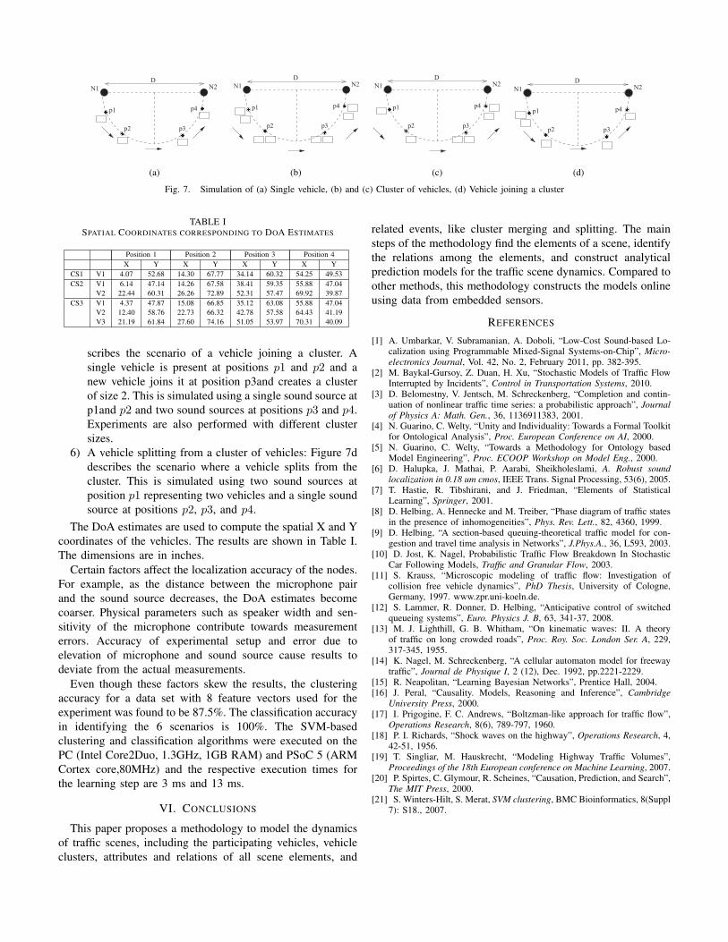
D

N1 N2

p1

p2 p3

p4

(a)

!!!!

!!!!

!! !

!!

D

N1 N2

p1

p2 p3

p4

(b)

! !!

!!!!

!

!!

D

N1 N2

p1

p2 p3

p4

(c)

! !!

!!!!

!

!!

D

N1 N2

p1

p2 p3

p4

(d)

Fig. 7. Simulation of (a) Single vehicle, (b) and (c) Cluster of vehicles, (d) Vehicle joining a cluster

TABLE ISPATIAL COORDINATES CORRESPONDING TO DOA ESTIMATES

Position 1 Position 2 Position 3 Position 4X Y X Y X Y X Y

CS1 V1 4.07 52.68 14.30 67.77 34.14 60.32 54.25 49.53CS2 V1 6.14 47.14 14.26 67.58 38.41 59.35 55.88 47.04

V2 22.44 60.31 26.26 72.89 52.31 57.47 69.92 39.87CS3 V1 4.37 47.87 15.08 66.85 35.12 63.08 55.88 47.04

V2 12.40 58.76 22.73 66.32 42.78 57.58 64.43 41.19V3 21.19 61.84 27.60 74.16 51.05 53.97 70.31 40.09

scribes the scenario of a vehicle joining a cluster. Asingle vehicle is present at positions p1 and p2 and anew vehicle joins it at position p3and creates a clusterof size 2. This is simulated using a single sound source atp1and p2 and two sound sources at positions p3 and p4.Experiments are also performed with different clustersizes.

6) A vehicle splitting from a cluster of vehicles: Figure 7ddescribes the scenario where a vehicle splits from thecluster. This is simulated using two sound sources atposition p1 representing two vehicles and a single soundsource at positions p2, p3, and p4.

The DoA estimates are used to compute the spatial X and Ycoordinates of the vehicles. The results are shown in Table I.The dimensions are in inches.

Certain factors affect the localization accuracy of the nodes.For example, as the distance between the microphone pairand the sound source decreases, the DoA estimates becomecoarser. Physical parameters such as speaker width and sen-sitivity of the microphone contribute towards measurementerrors. Accuracy of experimental setup and error due toelevation of microphone and sound source cause results todeviate from the actual measurements.

Even though these factors skew the results, the clusteringaccuracy for a data set with 8 feature vectors used for theexperiment was found to be 87.5%. The classification accuracyin identifying the 6 scenarios is 100%. The SVM-basedclustering and classification algorithms were executed on thePC (Intel Core2Duo, 1.3GHz, 1GB RAM) and PSoC 5 (ARMCortex core,80MHz) and the respective execution times forthe learning step are 3 ms and 13 ms.

VI. CONCLUSIONS

This paper proposes a methodology to model the dynamicsof traffic scenes, including the participating vehicles, vehicleclusters, attributes and relations of all scene elements, and

related events, like cluster merging and splitting. The mainsteps of the methodology find the elements of a scene, identifythe relations among the elements, and construct analyticalprediction models for the traffic scene dynamics. Compared toother methods, this methodology constructs the models onlineusing data from embedded sensors.

REFERENCES

[1] A. Umbarkar, V. Subramanian, A. Doboli, “Low-Cost Sound-based Lo-calization using Programmable Mixed-Signal Systems-on-Chip”, Micro-electronics Journal, Vol. 42, No. 2, February 2011, pp. 382-395.

[2] M. Baykal-Gursoy, Z. Duan, H. Xu, “Stochastic Models of Traffic FlowInterrupted by Incidents”, Control in Transportation Systems, 2010.

[3] D. Belomestny, V. Jentsch, M. Schreckenberg, “Completion and contin-uation of nonlinear traffic time series: a probabilistic approach”, Journalof Physics A: Math. Gen., 36, 1136911383, 2001.

[4] N. Guarino, C. Welty, “Unity and Individuality: Towards a Formal Toolkitfor Ontological Analysis”, Proc. European Conference on AI, 2000.

[5] N. Guarino, C. Welty, “Towards a Methodology for Ontology basedModel Engineering”, Proc. ECOOP Workshop on Model Eng., 2000.

[6] D. Halupka, J. Mathai, P. Aarabi, Sheikholeslami, A. Robust soundlocalization in 0.18 um cmos, IEEE Trans. Signal Processing, 53(6), 2005.

[7] T. Hastie, R. Tibshirani, and J. Friedman, “Elements of StatisticalLearning”, Springer, 2001.

[8] D. Helbing, A. Hennecke and M. Treiber, “Phase diagram of traffic statesin the presence of inhomogeneities”, Phys. Rev. Lett., 82, 4360, 1999.

[9] D. Helbing, “A section-based queuing-theoretical traffic model for con-gestion and travel time analysis in Networks”, J.Phys.A., 36, L593, 2003.

[10] D. Jost, K. Nagel, Probabilistic Traffic Flow Breakdown In StochasticCar Following Models, Traffic and Granular Flow, 2003.

[11] S. Krauss, “Microscopic modeling of traffic flow: Investigation ofcollision free vehicle dynamics”, PhD Thesis, University of Cologne,Germany, 1997. www.zpr.uni-koeln.de.

[12] S. Lammer, R. Donner, D. Helbing, “Anticipative control of switchedqueueing systems”, Euro. Physics J. B, 63, 341-37, 2008.

[13] M. J. Lighthill, G. B. Whitham, “On kinematic waves: II. A theoryof traffic on long crowded roads”, Proc. Roy. Soc. London Ser. A, 229,317-345, 1955.

[14] K. Nagel, M. Schreckenberg, “A cellular automaton model for freewaytraffic”, Journal de Physique I, 2 (12), Dec. 1992, pp.2221-2229.

[15] R. Neapolitan, “Learning Bayesian Networks”, Prentice Hall, 2004.[16] J. Peral, “Causality. Models, Reasoning and Inference”, Cambridge

University Press, 2000.[17] I. Prigogine, F. C. Andrews, “Boltzman-like approach for traffic flow”,

Operations Research, 8(6), 789-797, 1960.[18] P. I. Richards, “Shock waves on the highway”, Operations Research, 4,

42-51, 1956.[19] T. Singliar, M. Hauskrecht, “Modeling Highway Traffic Volumes”,

Proceedings of the 18th European conference on Machine Learning, 2007.[20] P. Spirtes, C. Glymour, R. Scheines, “Causation, Prediction, and Search”,

The MIT Press, 2000.[21] S. Winters-Hilt, S. Merat, SVM clustering, BMC Bioinformatics, 8(Suppl

7): S18., 2007.

Towards a Model-Driven Engineering Software Development Framework

Maxime Perrotin, Julien Delange and Samir BennaniEuropean Space Agency, TEC-SWE

Keplerlaan 12201AZ Noordwijk, The NetherlandsEmail: [email protected]

Abstract—Design and Implementation of Safety-Critical Sys-tems is becoming very difficult becauses it involves manyrequirements coming from different engineering domains. Dueto the increase of complexity, software of such systems can nolonger be produced with traditional methods, which show theirlimit over time. In that context, new development approacheshave to be introduced to avoid actual development traps andpitfalls. Among them, the Model-Driven Engineering approachconsists at representing system artifacts with models and auto-generate the code by refining them from high-level conceptsdown to the code. However, as for every new approach, it alsobrings new problems such as requirements consistency amongthe different notations (models) as well as integration issues (forexample, making sure that implementation code from differentmodels will behave correctly when merged on a single executionplatform).

This article presents our experience for integrating Guidanceand Navigation Control (GNC) algorithms designed with Ap-plication Models (Simulink) with Architecture Models (AADL).The process relies on code generator for both models andintegrate it on a typical execution platform. In particular,we focus on the challenges of the integration, illustrating thepractical problems we faced for producing a space system usinga Model-Driven Engineering Approach.

Keywords-AADL, TASTE, Simulink, MDE

I. INTRODUCTION

A. Context

Safety-critical systems are getting more complex, col-locating more functions on the same computing platform.As a consequence, their design becomes more complicated,leading to a long and potentially painful design process.Designers have to take into account requirements comingfrom different domains and specified with heterogeneousformalisms.

For that reason, producing the system using traditionalmethods is no longer feasible : checking impact betweenall requirements disseminated across different specificationsand notations is impossible, especially when the processis not automated. For that reason, new approaches mustbe designed. In our context, the Model-Driven Engineering(MDE) approach aims at separating system concerns inmodels, let engineers focus on their part of the systemwhile tools automate the integration and ensure consistenciesbetween modelling artifacts.

B. Problem

One key aspect of the MDE methodology is the sepa-ration of concerns: each engineer focuses on designing andimplementing his part of the system dedicated to his domainwhile specific tools process each implementation artifact,ensure their integration and preserve a semantic consistencybetween notations.

Despite having a clear separation between each domain,several problems remain when implementing a full MDEapproach. First of all, because of the use of different nota-tions, some requirements are sometimes captured twice indifferent models using heterogeneous notations. Then, toolsare expected to ensure their consistency but engineers arealso requested not to break them when manipulating models.Another issue is about simulation and implementation cor-rectness: even when a system was intensively tested usingsimulation functions, its integration as an implementationcode can generate a lot of errors. Most of the time, this isdue to the heterogeneous nature of the execution platform,whose environment is different from the simulation. Thus,having a dedicated process that ensures a smooth integrationof system functions by enforcing their behavior correctnessis a must.

In that context, to improve MDE approaches, it is worth-while to identify all traps and pitfalls in order to strengthenthe overall approach. Outcome of such investigations wouldmake tools more resilient to potential integration errors,the type of issue which is typically discovered just beforecompletion of a project, when few resources are available

C. Outline

The remainder of this paper is structured in two mainsections. The first one is an overview of the tools weuse: the TASTE toolset (Architecture modelling [1]), andSimulink [2] (Software modelling) and their integration.Second part of this paper presents our latest experimentsto design a spacecraft system using our MDE toolset bydesigning GNC algorithms on top of a distributed archi-tecture designed with TASTE. We provide a feedback abouttraditional traps and pitfalls of such integration, leading to anopen discussion about potential improvements of the wholeMDE development process.

II. BACKGROUND

A. Simulink

Simulink consists of a graphical modelling language anda set of tools for designing software (an example is shownin figure 2). It focuses on the definition of functionalconcerns and is mostly used to design algorithms in specificengineering domain (power control, navigation, etc.).

Simulink is a well-known and established tool, providingconvenient notation to abstract engineering concepts with auser-friendly simulation interface. Thus, it is a very efficienttool for engineers to prototype, design and implement theirpart of the system. In the context of the space industry, itis used in many engineering domains, from mechanical torobotics. In the present case-study, it was used to producethe GNC algorithms of a launcher.

B. TASTE

TASTE [3] is a project developed, maintained and sup-ported by the European Space Agency. It aims at providinga MDE toolset for the production of safety-critical systems.For that purpose, it defines the system using three views:

1) The Data View (DaV) specifies data types and encod-ing functions used to communicate between systemcomponents using the ASN.1 [4] language (see listing1 for an example). It corresponds to the externalinterfaces of the system, as specified in the ICD thatspecified all interfaces between the sub-systems (withtheir types, properties, etc.).

2) The Interface View (IV) enumerates system functions(what the system is doing), their requirements andconstraints (timing, data protection, etc.) and inter-actions among then (communication channels) usingthe AADL [5] language. Function connections refer-ence the Data View to specify types being used. Asthis model remains descriptive (a graphical sample isshown in figure 3), it has to be associated with codethat implements functions.

3) Deployment View (DeV) defines the execution plat-form (processors, buses, etc.) of the system, its con-figuration as well as deployment of functions (fromthe Interface View) into it. It also uses the AADL [5]for that purpose, an example is shown in figure 4.

These models are processed with their functional code toautomatically produce system implementation (as shown infigure 1) through the following steps:

• The Data View is translated into declarations (datatypes, functions) in the target code (C, Ada, etc.) so thatwe can use the same interfaces with different languages.

• The Interface and Deployment Views are processed tocreate an architecture code that supports the executionof the functional code. This aims at creating andconfiguring resources (tasks, mutexes, etc.) that reflect

requirements specified in the interface view (period,deadline, etc.).

• The Integration Process compiles the functional codefrom the user with the architecture code generatedfrom models, producing the program to be deployedon the execution target. This code is also automaticallytailored to the target operating system. As for now, ourtoolchain supports several architecture (x86, SPARC,etc.) and different Operating System for safety-criticalsystems such as Linux or RTEMS [6].

FIGURE 1: TASTE development process

C. Integration of Software Models into Architecture ModelsOur process (figure 1) automatically deploys application

code (written by domain-specific users, such as electri-cal/mechanical engineers) on top of architecture code. Theformer can be designed using either regular (C, Ada) ormodelling (Simulink, SDL, etc.) languages. Our toolchainautomatically generates glue code that connects functionalblocks, enabling communication between code written withdifferent languages and executed on heterogeneous architec-tures.

However, when integrating application models (such asSimulink), algorithms requirements must comply with thearchitecture constraints (timing requirements of the Inter-face View, interfaces definition of the Data View, etc.). Us-ing a traditional, manual integration, no check is performed,lack of compliance between models is discovered either afterintegration (at best), or during execution (at worst). Thefollowing section contains the description of a complete casestudy we conducted in order to experiment and validate theuse of a model-based approach with the TASTE tools.

III. CASE-STUDY AND FEEDBACK

A. OverviewIn order to validate our approach and tools, we have built a

system to support the validation of the navigation algorithms

(GNC) of a onboard launcher software. In that context, wehave developed (or reused) a large set of Simulink modelsthat represent the environment of the software: the sensorsand actuators on one side, and the flight dynamics on theother side. This way we have the means to generate realisticdata at runtime to feed the control laws and run in closedloop.

On the other side, we have the flight code of the controllaws in Ada language. The challenge is to put both piecestogether, and make them run on different platform: firstnatively on Linux to test the integration, and later on amixed platforms (x86/Linux for the environment models,and Sparc/Leon for the control law running in real-time). Atruntime, we want to observe data and plot the control laws’main parameters. TASTE provide the means to achieve thesegoals.

B. Application modelling

FIGURE 2: Simulink model of our case-study

Modelling the application with TASTE was done in threesteps

1) specify the data types in ASN.1 to describe the mes-sages exchanged between our functions (listing 1)

2) capture the logical architecture of the system (figure3) into an Interface View that references the Simulinkmodel (shown in fig:simulink-model).

3) model the deployment of the application, by mappingthe functions onto hardware components, and connectthem with buses (figure 4).

From these models, TASTE generate skeletons, that con-sist in empty code blocks that would contain the application(Simulink models). Once these code blocks have been filledby the user, tools automatically create all the glue code thatis necessary to implement the system (communication, etc.)without having to manually tweak the interfaces. This auto-connects blocks from different implementation languages(Ada, C, Simulink, etc.) smoothly, without having to changethe communication mechanisms. Using these tools gave usguarantee that there would be no inconsistencies in datarepresentation for each block. This allows to start running

simulations very quickly and make rapid prototyping ofembedded application without having to tweak applicationcode.

VEGA DEFINITIONS : : =BEGINT−GNC−LV−SIM−CONTEXT : : = SEQUENCE {

a t t i t u d e−q u a t e r n i o n T−QUAT−FLOAT32 ,ng−ve l−i n c r− i r s T−VECT3−FLOAT32 ,ng−ve l−i n c r−a c c e l e r o T−VECT3−FLOAT32 ,f i l t e r e d −a n g l e s−sample−1 T−VECT3−FLOAT32 ,f i l t e r e d −a n g l e s−sample−2 T−VECT3−FLOAT32

}

T−GNC−LV−SIM−INPUTS : : = SEQUENCE {sequ−exec−r e q u e s t−v e c t

T−HAS−SEQUENCE−EXEC−BEEN−REQUESTED−VECT,tvc−s e t−p o i n t−eng−v e c t

T−TVC−SET−POINT−ENG−VECT,r a c s−ev−cmd−v e c t

T−RACS−EV−CMD−VECT}

T−QUAT−FLOAT32 : : = SEQUENCE( SIZE ( s i z e−T−QUAT−COMPONENTS) ) OF T−FLOAT32

# . . .END

Listing 1. Data View of our case-study

FIGURE 3: Interface View of our case-study

C. Feedback

The experience gives us the ability to produce a large scalelauncher simulator that we are now running to cross-checkthe control laws of our launchers. Until now, we did most ofthese simulations entirely within the Matlab/Simulink envi-ronment. It is also a very powerful and effective approach;the drawback is that the execution is not representative ofreal targets, and that the integration of the code later on inthe real onboard software can become much more difficultwhen done at a later stage. Using automated tools to makethe models and code integration from the very early stages

of the development brings significant added value and makesthings simpler to integrate for non-software people.

However, we experienced two major issues when in-tegrating Simulink code on the real target. First of all,the generated code from application models is not fullyconsistent with the models specification, leading to errorsthat were not seen during simulation. This brings us todebug the generated code by hand to discover the problem.This should be automatically detected by the tools. Also,another issue was the programming skills of engineers : thetoolchain required adaptation of existing Simulink modelsto the TASTE interface. This job requires some modelrefactoring to fit TASTE and Simulink models and was noteasy for non computer-scientist engineers. As a result, wespent a lot of time explaining the design process to engineersso that they can use our toolchain.

IV. CONCLUSION

This article presents our feedback about the issues of thedeployment of software models with architecture, particu-larly regarding potential errors that are introduced during theintegration phase, at the latest phases of system production.These experiments were done in the context of internalprojects at the European Space Agency, while integratingGNC algorithms (designed and tested usign simulation func-tions from Simulink) with an execution runtime.

These issues convince us to strenghthen the overall de-velopment process and propose new functionalities thataim at checking system compliance between execution andsimulation. For example, being able to monitor systeminterfaces and check correctness between simulation andexecution would help developers but also support the overalldevelopment process, providing artifacts required for systemvalidation.

A. Perspectives

Verification between models could also be introduced ear-lier in the development process, prior to system integration.For example, it would be possible to check compliance be-tween heterogeneous models before generating or integratingcode. This engineering effort, even if technically feasible,would require a static analysis of the model, which requiresa huge maintainance effort due to the number of applicationlanguages supported by our toolchain.

sectionAknowledgmentThe authors would like to thank the VEGA project and

the TEC-ECN and TEC-SW laboratories for their supportand contributions to this paper.

ACRONYMS

ASN Abstract Syntax NotationICD Interface Control DescriptionGNC Guidance and Navigation ControlMDE Model-Driven Engineering

TASTE The ASSERT Set of Tools for Engineering

FIGURE 4: Deployment View of our case-study

REFERENCES

[1] L. Bass, P. Clements, and R. Kazman, Software Architecture inPractice, ser. SEI Series in Software Engineering. Addison-Wesley, 2003.

[2] O. Beucher, MATLAB und Simulink (Scientific Computing).Pearson Studium, 08 2006.

[3] M. Perrotin, E. Conquet, J. Delange, T. Tsiodras, andA. Schiele, “TASTE A real-time software engineering tool-chain,” in Proceedings of the 15th International Conferenceon System Design Languages, 07 2011.

[4] O. Dubuisson, ASN.1 Communication entre systemesheterogenes: Guide d’utilisation, manuel de reference, ser.Collection Technique Et Scientifique Des Telecommunications.Springer, 1999.

[5] As-2 Embedded Computing Systems Committee SAE, “Archi-tecture Analysis & Design Language (AADL),” SAE Standardsno AS5506, November 2004.

[6] “RTEMS : Real-Time Operating System for MultiprocessorSystems,” http://www.rtems.com.

http://www.rtems.com

Integration of Mixed-Criticality Cyber-Physical Systems with Criticality Layers

Dionisio de NizSEI - Carnegie Mellon University

Pittsburgh, PA, [email protected]

Anthony RoweECE - Carnegie Mellon University

Pittsburgh, PA, [email protected]

Abstract—Large Cyber-Physical Systems such as avionicsand automotive systems often require large integration effortsbetween third-party components. These components providefunctionality at different levels of criticality yet share manyof the same underlying resources (CPU, Memory, Network,Disk, Transducers). As a result, protections mechanisms areneeded to prevent lower-criticality task from interfering withhigher-criticality ones. In this paper, we discuss how traditionaltemporal protection mechanisms such ARIC 653 partitions failto fully protect high-criticality tasks from lower-criticality ones.We then show how the Zero-Slack QRAM scheduler (ZS-QRAM) can be used in multi-layer systems to avoid theseproblems. Furthermore, we propose the use of criticality layersbased on the asymmetric protection scheme of ZS-QRAM inorder to simplify this integration, increase its robustness, andreduce its resource usage. Finally, we discuss some open issuesthat need to be addressed in order to remove some of thelimitations of this approach.

I. INTRODUCTION

In modern Cyber-Physical Systems (CPS), such as avion-ics and automotive systems, there is increasing pressure toreduce cost while increasing functionality and managingphysical resources like power and heat. This has resultedin the consolidation of functionality of different componentsinto shared hardware resources (e.g. processor and memory).Unfortunately, such sharing can lead to interference acrosstasks (e.g. one task using the processor longer than expected)each of which may have different criticality requirementsfor the system. For instance, if we deploy an ABS brakingsystem task on the same processor as a navigation systemtask of the car, if the latter does not release the processoron time it could make the former miss its deadline. Thisproblem is a concern of growing interest and has spawnedinitiatives to investigate building blocks that can be used tosafely construct mixed-criticality systems like the Mixed-Criticality Architecture Requirements (MCAR) [1] as wellas standards like ARINC-653 [2] and ISO-26262 [3].

Copyright 2012 Carnegie Mellon University and IEEEThis material is based upon work funded and supported by the Depart-

ment of Defense under Contract No. FA8721-05-C-0003 with CarnegieMellon University for the operation of the Software Engineering Institute,a federally funded research and development center.

This material has been approved for public release and unlimited distri-bution.

Carnegie Mellon is registered in the U.S. Patent and Trademark Officeby Carnegie Mellon University. DM-0000062

The consolidation of mixed-criticality systems demandsthe temporal protection of critical functionality. Traditionalapproaches such as ARINC 653 offer a symmetric protectionscheme where not only higher-criticality functionality isprotected from lower-criticality one but also lower-criticalityis protected from higher-criticality one. Unfortunately, thistype of protection can lead to criticality inversion, i.e., lower-criticality tasks blocking a higher-criticality one. Specifi-cally, symmetric protection can stop a higher-criticality taskif it tries to run longer that its allocated budget in orderto allow a lower-criticality task to run. In contrasts, Zero-Slack Rate-Monotonic (ZSRM) scheduling [4] provides anasymmetric protection scheme where a lower-criticality taskcan be stopped in order to ensure that higher-criticalitytasks meet their deadline but a lower-criticality task cannotinterfere with higher-criticality ones. The Zero-Slack QoSResource Allocation Model-based (ZS-QRAM) [5] sched-uler extends this concept even further to systems where taskscan have the same level of criticality but provide differentutility to the user. In this case, when an overload occurs,the lower-utility tasks are degraded to a lower executionrate (longer periodicity) to allow higher utility tasks to keepexecuting at a high rate.

We believe that asymmetric temporal protection shouldbe the norm when integrating mixed-criticality CPS. Thistype of protection enables the creation of criticality layersthat support layered certification standards like DO-178C [6]and ISO-26262 [3]. In this paper, we present a layeredarchitecture based on the asymmetric temporal protectionof ZS-QRAM and related mechanisms to support differentaspects of the applications. Finally, we discuss the issuesthat still need to be addressed to provide a comprehensivesolution.

II. ZS-QRAM

In this section, we provide background information relatedto ZSRM and ZS-QRAM as a basis for our discussion onusing it in a layered manner. ZSRM is a fixed-priority pre-emptive scheduling approach for uniprocessors. In ZSRM,a criticality value (ζi) is associated with each task τi toreflect the task’s importance to the safety of the CPS1.

1Our convention is to use lower values to indicate higher criticality.

These tasks are periodic with a period Ti, an implicitdeadline at the end of the period, and two execution times.The first execution time is considered the WCET during anominal mode of operation, called Nominal-Case ExecutionTime (Ci), and the other is called the Overloaded-CaseExecution Time (Co

i ) that is considered the WCET duringan overload situation (e.g. when the number of objects toavoid is unusually large). ZSRM works on top of traditionalpriority-based preemptive real-time schedulers. It is based onthe observation that criticality inversion only matters underoverload conditions. We use this observation to create twoexecution zones for each task τi. In the first zone, everytask is allowed to execute as normal, while in the secondzone, every task τj |ζj > ζi is suspended. This suspensioneffectively blocks the interference of lower-criticality tasksin the case of an overload condition, up to the completionof the task activation. It must be noted that τi itself canalso be suspended by a task τc|ζc < ζi in τc’s second zone.The execution zones partition the execution of each task intotwo modes: the normal mode (N mode) and the critical mode(C mode). Our scheduling algorithm then calculates the lastinstant at which a task can suspend lower-criticality tasks inorder to finish before its deadline. This instant is known asthe zero-slack instant (Zi) and is used at runtime to setupa timer when a job Ji,k from τi arrives. If such an timerexpires, then the lower-criticality tasks are suspended, butif Ji,k finishes before the timer expires, then no suspensionis performed and the lower-criticality tasks are allowed tocontinue.

ZS-QRAM builds upon ZSRM by adopting mechanismsfrom the Quality-of-Service (QoS) Resource AllocationModel (Q-RAM) [7]. Q-RAM uses utility functions thatdescribe the different QoS levels that tasks can obtain alongwith the resources (e.g., processor time) that they consumeand the utility that the user derives from each QoS level. Insimple configurations, Q-RAM primarily takes advantage ofthe fact that as applications (e.g. video streaming) increasetheir QoS level, the incremental utility to the user decreases.This is known as diminishing returns. For instance, in avideo streaming application increasing the frames per secondfrom 15 to 20 gives the user higher utility (i.e., perceivedquality) than increasing from 20 to 25 frames per second.Q-RAM uses the utility functions to perform a near-optimalallocation of resources to different tasks exploiting thediminishing returns property. In particular, the diminishingreturns property manifests itself in these functions as amonotonically-decreasing utility-to-resource ratio. This ratiois know as marginal utility. Q-RAM uses the marginal utilityto perform the allocation one increment at a time startingwith the increment that derives the largest utility for thesmallest allocation of resources (largest marginal utility).In each of the subsequent steps, it selects the next largestmarginal utility increment until the entire resource (e.g. CPUutilization) has been allocated. In the ideal case, the marginal

utility of the last allocation (QoS level) of all the tasks isthe same.

ZS-QRAM is designed for tasks whose different QoSlevels are implemented using different task periods. Task pe-riods are mapped to allocation points in the utility functions.ZS-QRAM first considers utility functions based on the Ci

of the tasks, and utilizes Q-RAM to do an initial allocationwhere each increment in the allocation is represented by anincreasingly shorter period. If a task overloads at runtime,an overload management mechanism is used to degradetasks (by selecting a longer period) to keep the tasksetschedulable. This mechanism uses task utility functionsbased on their Co

i to select the tasks that render the leastutility per unit of CPU utilization (marginal utility).

ZS-QRAM supports an admission test that uses two steps.First, it performs an initial Q-RAM allocation using thenominal marginal utility of the tasks. In other words, itbuilds utility functions assuming tasks run for their Ci

and follows the Q-RAM allocation order until the availableCPU utilization is fully allocated. Second, once the Q-RAMallocation is completed, the ZS instant Zi of each task τi iscalculated. This instant is then used to degrade tasks τj withlower utility than τi. To support this degradation, tasks arestructured as a set of task modes with different utility andthe degradation is configured as a mode transition.

III. ZS-QRAM LAYER HIERARCHY

ZS-QRAM embeds both the criticality-based and theutility-based scheduling and enforcement policies. Sincethe criticality-based policy has precedence over the utility-based one, they form layers where tasks scheduled based oncriticality have precedence over tasks scheduled based onutility. We identify these layers as the criticality layer andthe utility layer respectively.

The criticality layer is divided into multiple sub-layers(called simply layers when appropriate) based on criticalitylevels (used in the taskset). Criticality layers provide twoimportant properties that simplifies the integration of mixed-criticality systems: layer isolation, and layer overbooking.Layer isolation guarantees that a higher-criticality layercannot be affected by a lower-criticality layer. In otherwords, every task τi in a high-criticality layer are guaran-tee to execute for Co

i before its deadline whether or notlower-criticality layers exist. This implies that these lower-criticality layers can be added on top of higher-criticalityones without compromising their guarantees. On the otherhand, layer overbooking allows layers of different criticalityto share CPU cycles increasing the system capacity to fitmore features. In this case, the lower criticality layer usesthese shared cycles (meeting its deadline) if no task τj in thehigher criticality layer exceeds its nominal execution timeCj . This overbooking allows an efficient and safe resourcesharing across criticality layers. It is worth noting that both

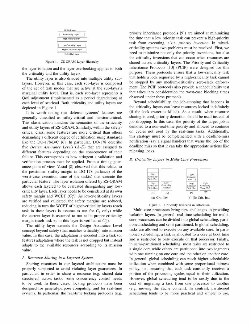
Critcality Layer

Utility Layer

High-Critcality Layer

Low-Critcality Layer

High-Utility Layer

Low-Utility Layer

Figure 1. ZS-QRAM Layer Hierarchy

the layer isolation and the layer overbooking applies to boththe criticality and the utility layers.

The utility layer is also divided into multiple utility sub-layers. However, in this case, each sub-layer is composedof the set of task modes that are active at the sub-layer’smarginal utility level. That is, each sub-layer represents aQoS adjustment (implemented as a period degradation) ateach level of overload. Both criticality and utility layers aredepicted in Figure 1

It is worth noting that defense systems’ features aregenerally classified as safety-critical and mission-critical.This classification matches the semantics of the criticalityand utility layers of ZS-QRAM. Similarly, within the safety-critical class, some features are more critical than othersdemanding a different degree of certification suing standardslike the DO-178-B/C [6]. In particular, DO-178 describefive Design Assurance Levels (A-E) that are assigned todifferent features depending on the consequence of theirfailure. This corresponds to how stringent a validation andverification process must be applied. From a timing guar-antee point-of-view, Vestal [8] observed that this relates tothe pessimism (safety-margin in DO-178 parlance) of theworst-case execution time of the task(s) that execute theparticular feature. The layer isolation offered by ZS-QRAMallows each layered to be evaluated disregarding any low-criticality layer. Each layer needs to be considered at its ownsafety margin and WCET (Co

i ). As lower-criticality layersare verified and validated, the safety margins are reduced,reducing in turn the WCET of higher-criticality layers (eachtask in these layers is assume to run for Ci only) whilethe current layer is assumed to run at its proper criticalitymargin (each task τj in this layer is verified at Co

j ).The utility layer extends the Design Assurance Level

concept beyond safety (that matches criticality) into missionvalue. In this case, the adaptation is encoded into a task (orfeature) adaptation where the task is not dropped but insteadadapts to the available resources according to its missionvalue.

A. Resource Sharing in a Layered System

Sharing resources in our layered architecture must beproperly supported to avoid violating layer guarantees. Inparticular, in order to share a resource (e.g. shared datastructures) across tasks, some concurrency control needsto be used. In these cases, locking protocols have beendesigned for general-purpose computing, and for real-timesystems. In particular, the real-time locking protocols (e.g.

priority inheritance protocols [9]) are aimed at minimizingthe time that a low priority task can prevent a high-prioritytask from executing, a.k.a. priority inversion. In mixed-criticality systems two problems must be resolved. First, weneed to minimize not only the priority inversions, but alsothe criticality inversions that can occur when resources areshared across criticality layers. The Priority-and-CriticalityInheritance Protocols [10] (PCIP) were designed for thispurpose. These protocols ensure that a low-criticality taskthat holds a lock requested by a high-criticality task cannotbe stopped by any medium-criticality zero-slack enforce-ment. The PCIP protocols also provide a schedulability testthat takes into consideration the wost-case blocking timesobserved under these protocols.

Beyond schedulability, the job-stopping that happens inthe criticality layers can leave resources locked indefinitely(if the lock owner is killed). As a result, when resourcesharing is used, priority demotion should be used instead ofjob dropping. In this case, the priority of the target job isdemoted to a non-real-time priority and allowed to continueon cycles not used by the real-time tasks. Additionally,this strategy must be complemented with a deadline-missnotification (say a signal handler) that warns the job of thedeadline miss so that it can take the appropriate actions likereleasing locks.

B. Criticality Layers in Multi-Core Processors

(a) Crit. Inv. (b) No Crit. Inv.

Figure 2. Criticality Inversion in Allocation

Multi-core processors bring new challenges to providingisolation layers. In general, real-time scheduling for multi-core processors can be divided into global scheduling, parti-tioned scheduling and semi-partitioned. In global scheduling,tasks are allowed to execute on any available core. In parti-tioned scheduling, a task is allocated to a core at boot timeand is restricted to only execute on that processor. Finally,in semi-partitioned scheduling, most tasks are restricted toa single core while others are partitioned into two segmentswith one running on one core and the other on another core.In general, global scheduling can reach higher schedulableutilization when combined with some proportional fairnesspolicy, i.e., ensuring that each task constantly receives aportion of the processing cycles equal to their utilization.However, global scheduling tend to be costly due to thecost of migrating a task from one processor to another(e.g. moving the cache content). In contrast, partitionedscheduling tends to be more practical and simple to use,

but it may suffer from fragmentation cost due to unusedutilization of a processor (where no single task can fit).However, in practice this fragmentation is rare and for safetycritical systems, the simplicity of a partitioned approach ishighly desirable. For this reason, we propose the use ofpartition scheduling for layered mixed-criticality systems.

In partitioned scheduling of mixed-criticality systems, thecriticality inversion problem can arise at the task-allocationlevel. A given allocation could favor a low-criticality task atthe expense of a high-criticality one. For instance, considerthree tasks τh1, τh2, and τl of high, high, and low criticalityrespectively, each having a normal utilization Ci

Tiof 40%

. Assuming we only have two processors P1 and P2, andτh1 is already deployed on P1, and the three tasks donot fit on P1 together, then we are forced to pack eitherτh2 or τl on P1 and the other to P2. Packing τh1 andτh2 together, and τl by itself is a possible task allocationdecision (see Figure 2(a)). In fact such an allocation decisionis commonly used in legacy systems that try to isolatecriticality levels. However, observe that such task allocationleads to a criticality inversion problem. In this scenario,if all the tasks overload, τh2 may miss its deadline butτl will not i.e. our allocation decision protected τl (a lowcriticality task) at the expense of τh2 (a high criticality task).Conversely, deploying τh1 and τl together and τh2 by itselfremoves this criticality inversion (see Figure 2(b)). Note thatusing a criticality-aware uniprocessor scheduling algorithmsuch as ZSRM will ensure that τl cannot steal cycles fromτh1 within processor P1 under overload scenarios.

In [11] we developed a mixed-criticality task allocationalgorithm called Compress-on-Overload Packing (COP) thatfirst allocates the highest-criticality tasks as if they wererunning for its overloaded execution time Co

i . Once theprocessors are full, it then recalculates the allocated utiliza-tion of the processors as if the tasks were now running fortheir nominal execution time Ci. Finally, the lower-criticalitytasks are packed “on top” of the previously allocated tasks.It is worth noting that this scheme allocates the tasks incriticality layers, from the highest to the lowest criticality.This packing highlights the advantage of sharing resourcesbetween low and high criticality tasks.

IV. OPEN ISSUES

Asymmetric protection for mixed-criticality systemsneeds to be extended across other subsystems of the com-puting platform to act as a comprehensive solution. Areascurrently not covered include: the Input-Output subsystemsincluding interrupts, DMA, and lower-level sensors andactuations. In distributed systems, protection mechanisms fornetwork bandwidth would also be required. In the multi-core arena, resources shared across cores such as cacheand memory banks require new mechanisms for asymmetrictemporal protection. Finally, the mixed-criticality synchro-nization protocols need to be extended for multiprocessors

(and multicores).

V. CONCLUDING REMARKS

In this paper, we proposed the use of the asymmetric tem-poral protection of ZS-QRAM to integrated mixed-criticalityCPS in a layered architecture. We presented the differentmechanisms that ZS-QRAM uses to build a hierarchy ofcriticality layers and the advantages of this hierarchy for thecertification of these systems in the light of safety standardslike the DO-178C. In addition, we presented the mechanismsto support resource sharing within and across criticalitylayers. We discussed the criticality inversion problem inpartitioned multiprocessor scheduling and our allocationalgorithm designed to minimize it. Finally, we discussedthe open issues that need to be addressed in order toprovide a comprehensive solution. In the end, we believe thatthe layered architecture presented here and the supportingmechanisms provide a strong design platform for mixed-criticality systems that is well aligned with the philosophy ofthe certification authorities facing commercial and militaryCPS.

REFERENCES

[1] D. Homan, “Designing future systems for airworthiness cer-tification,” http://www.cse.wustl.edu/∼cdgill/CPSWEEK09MCAR/, 2009.

[2] Avionics Application Software Standard Interface, ARINCStd. 653p1-2, 2005.

[3] ISO, “Road vehicles – functional safety,” http://www.iso.org/iso/catalogue detail.htm?csnumber=43464.

[4] D. de Niz, K. Lakshmanan, and R. Rajkumar, “On thescheduling of mixed-criticality real-time task sets,” in RTSS2009, dec. 2009.

[5] D. de Niz, L. Wrage, N. Storer, A. Rowe, and R. R. Rajkumar,“On resource overbooking in an unmanned aerial vehicle,” inICCPS, 2012.

[6] S. C. of RTCA, “DO-178C, software considerations in air-borne systems and equipment certification,” 2011.

[7] R. Rajkumar, C. Lee, J. Lehoczky, and D. Siewiorek, “Aresource allocation model for qos management,” in RTSS, dec1997.

[8] S. Vestal, “Preemptive scheduling of multi-criticality systemswith varying degrees of execution time assurance,” In Pro-ceedings of RTSS, pp. 239–243, 2007.

[9] L. Sha, R. Rajkumar, and J. Lehoczky, “Priority inheritanceprotocols: an approach to real-time synchronization,” Com-puters, IEEE Transactions on, vol. 39, no. 9, Sep 1990.

[10] K. Lakshmanan, D. de Niz, and R. R. Rajkumar, “Mixed-criticality task synchronization in zero-slack scheduling,” inProceedings of the IEEE RTAS, 2011.

[11] K. Lakshmanan, D. de Niz, R. R. Rajkumar, and G. Moreno,“Resource allocation in distributed mixed-criticality cyber-physical systems,” ICDCS, 2010.

Analytic Certification Technologies

for Military Avionics

Russell B. Kegley and Jonathan D. Preston

Lockheed Martin Aeronautics Company

Fort Worth, Texas, USA

{russell.b.kegley, jonathan.d.preston}@lmco.com

Abstract� Historic approaches to upgrading the capabilities of

military aircraft by inserting new technologies have become so

costly that warfighters may be forced to operate with less than

current technology can deliver. Even inserting new upgrades

alongside the legacy systems can be very expensive if it requires

large modifications to legacy software, triggering extensive retest.

A way to meet this challenge is to insert upgrades alongside

legacy systems, virtually replacing old capabilities with new while

leaving the old software in place. This approach carries with it

new challenges which might be met with analytic innovations.

Keywords-component; incremental upgrade, embedded

avionics, timing, specification, reuse, verification, validation,

complexity

I. INTRODUCTION

Increasingly, the lifetimes of military aircraft platforms are exceeding 40 years. Modernization of the basic airframe in the form of better engines or strengthened components is a well-understood practice. However, the industry must find new paths for upgrading software-provided capabilities. Past approaches accomplished mission software and hardware upgrades by essentially removing the old components and replacing them with entirely new systems inserted into the existing airframe. Budget realities going forward make this an unaffordable model, making it essential to be able to continue to use some functions from the legacy system while inserting new or updated capabilities alongside them. Accomplishing these incremental system upgrades challenges the analytical frameworks that defense contractors have relied on to date to ensure predictable, bounded integration times and costs, and to generate performance and deadline guarantees required for system acceptance. In this position paper, we outline the problem and point to specific challenges which we believe are key technologies required to meet them.

II. MISSION AVIONICS UPGRADES: THE PAST

Past approaches to mission avionics upgrades have followed a few general approaches. Figure 1 shows a typical legacy mission avionics system, in which the primary software domains (Controls, Displays, Weapons, etc.) are distributed over a set

of computing nodes; typically the nodes have nearly identical processing technology, with some differences to accommodate specialized I/O. The domains usually have well-defined boundaries which often correspond to hardware boundaries, meaning that changes can be localized fairly narrowly. The paper by Seeling [1] gives a fairly rare published detailed view of a specific avionics system in the context of reconfiguration options; most such system descriptions are not readily available.

Over a period of 7-15 years after an aircraft has been introduced, the industry develops new technologies and enhanced capabilities which start appearing in new products, but which are not available in the older aircraft. During this time, military customers create a body of experience and knowledge of how to use the aircraft in actual missions, and also discover functions which, if added to the aircraft, would make it better-suited to their needs. The defense purchasing community and the aircraft manufacturers jointly identify a set of capabilities to be introduced, and create a procurement program which involves removing the existing mission avionics system and replacing it in toto with a newly-developed set of hardware and software. While this new system almost always contains the same capabilities as the old software, these

Figure 1. Legacy missions avionics system

functions may be expressed in new forms, and of course the new system has additional functions which were not present in the system. Since the end product is a complete replacement, there are few backward compatibility issues to be handled. The new capabilities are typically well-crafted into the user interface, and in most respects the integration is not much harder than a complete new product would be.

Procurement bodies and contractors have long recognized that this is not the most desirable scenario, and have proposed others. The overriding concern, as noted by Duren [2] is to minimize changes to existing software, since this incurs the greatest expense. One approach proposed by Luke et al., RePLACE, uses emulation to rehost legacy software unchanged on a newer, faster processor [3]. While this method lets the integrator continue to use old software without change, and provides the CPU power to support new functions, it was not primarily concerned with the issues involved in making the new work with the old. An alternative to executing the legacy software unchanged is to simply port it in a functionally-unchanged form to the new environment; an extreme example of this is discussed in Murray [4], where assembly language code for an obsolete processor is ported to the new system. It is hard to imagine this scenario being affordable today.

The primary obstacle to continuing to do wholesale system upgrades is that while it is easier in some ways, complete mission hardware and software replacements are very expensive; forecasts for defense spending seem to rule out most of these upgrades in the future. The high cost also has another, even more important downfall: when capability upgrades are delayed for years or perhaps decades because of budget constraints, warfighters are faced with the prospect of having to conduct their missions with less capability than the technology would allow.

III. MISSION AVIONICS UPGRADES: A POSSIBLE FUTURE

A great deal of the cost associated with the upgrade practice just discussed is the result of completely replacing all of the hardware and software systems. In many cases, the old functions may have been sufficient even with new capability insertions, but the replacement approach rewrites that software so it can be hosted on the new hardware. The cost escalates � � � � � � � � � � � � � � � � � � � � � � � � � � � � � � � � � � � � � � � � � � � � � �simply replace existing functions which were still adequate, must be exhaustively tested.

Performing future upgrades could be made more affordable by carefully matching current capabilities against the desired capabilities and finding ways to keep those functions in the current system which still meet the new mission requirements. Leaving much of the current system in place and simply adding new software capabilities and hardware could eliminate a large part of the upgrade cost. Figure 2 shows this scenario in the context of a proposed refresh of a radar subsystem; this is a fairly common replacement as radar hardware and a software technology advance, and represents a great increase in warfighter capability. As shown, updating the radar involves accommodating the new temporal architecture the subsystem � � � � � � � � � � � � � � � � � � � � � � � � � � � � � � � � � � � � �

en to bridge this difference. Since the radar brings new capabilities which replace earlier functions dependent on the old radar subsystem, a new sequence of function calls or object method invocations is created on the inserted system which renders the earlier function void. In this proposed upgrade scenario, the old radar mission thread software is not removed from the legacy software; it is simply no longer exercised by any stimulus, rendering it virtually removed.

The new capabilities are of course hosted on an updated computing node, which may have a different operating system and middleware, perhaps reused from a newer military aircraft

Figure 2. Proposed more affordable upgrade practice

program. This introduces the need to analytically demonstrate the harmony of fault logic and handling across the now-diverse architecture.

IV. KEY CHALLENGE AREAS

Moving from the costly historical upgrade practices to a future practice which leaves still-functional software in place, and which virtually removes unneeded code instead of modifying the source, presents several challenges, which we detail below.

Temporal Architecture Differences The temporal architectures of the legacy and new functions may be vastly different. This difference could be relatively easy to bridge, like an old cyclic execution rate of 50Hz vs. a rate of 75Hz in the new software. However, the new software could be based on an event-driven paradigm which assumes immediate transmission of messages with an implied wait for response, such as a remote procedure call. This kind of difference may require more careful analysis, or cause changes to some of the � � � � � � � � � � � � � � � � � � � � � � � � � � � � � � � � � � � � � � � � � � � � deadlines. Thus, in some cases the new function might be able to be recast into the temporal vocabulary of the legacy behaviors, but whe

� � � � � � � � � � � � � � � � � � � � � � � � �components originally developed for some other system, it might be required to use the new functions as-is and somehow harmonize the different temporal architectures.

Unused Code The idea of leaving some legacy code in-place while virtually turning off its execution is a novel one for military systems. Current standards for safety- or mission-critical applications call for physically removing all code that is not actually executed; a key enabler to an affordable increme

� � � � � � � � � � � � � � � � � � � � � � � � � � � � � � � � � � �� exercised in the upgraded system while still leaving it in place in the legacy portion of the aircraft.

Application Architecture and Design Styles New applications likely employ different structuring approaches than legacy applications stemming from differences in programming languages, differences in computing resource constraints, and provisions for long term maintainability. Such differences come into play when it is desired to re-use legacy application code in part, or integrate software components from different suppliers. Reconciling differences can result in � � � � � � � � � � � � � � � � � � � � � � � � � � � � � � � � � � � � � � � � � � � � � � � � � �and new components.

Communication Protocol Differences Applications typically communicate across the avionics architecture using messages. However, there can be great variety in the types and styles of communication and handshaking approaches used across different generations of applications. Different schemes include: Asynchronous unacknowledged messages, acknowledged delivery, remote procedure call (RPS), singlecast and multicast. Client/server and subscription based approaches have also been used.

Infrastructure Code and Support Services Applications from different eras and suppliers often have different infrastructure software requirements and assumptions,

including those related to: operating system, security requirements, support libraries, load and startup, and persistent data storage, and scheduling.

Difference in Fault Tolerance Designs Generally, there are fault tolerance and system reliability requirements levied on avionic systems. Incremental upgrades need to be mindful of potential differences in fault detection, isolation, and response schemes. Often, fault tolerant designs are based on assumptions established very early in the initial design. Sometimes, documentation of requirements and underlying assumptions is lacking, and this can introduce risk as new functionality is added. Additionally, fault tolerance designs generally require full regression testing, even when the scope of intended design change is small and well known.

Documentation Coverage and Quality The behaviors of the legacy system may be incompletely documented or � � � � � � � � � � � � � � � � � � � � � � � � � � � � � � � � � � � � � � � � � � functional perspective may be so entwined that it is difficult to find ways to virtually sever the legacy system into behaviors that will continue to be exercised in the upgraded system and those that will be replaced by newly inserted technology.

V. CONCLUSIONS

We present a potentially more affordable route for inserting technology upgrades into military aircraft. While this approach avoids replacing existing, still-functional software, it carries with it new challenges that require analytical methods yet to be developed and proven. As Table I shows, the gap between legacy hardware, software infrastructure, and application designs can be large.

TABLE I. HISTORIC VS. FUTURE UPGRADE SUMMARY

Legacy System Future System

Processing

hardware

Single CPU per subsystem

Military-specific instruction set

Single- � � � ! " # $ %

Multiprocessor subsystems ! � & & � � ' ( ) ! " # $ %(suitably hardened)

Multicore technology

Operating

systems

Custom developed

Fixed rate scheduling

Timesliced temporal architecture

Commercial high assurance RTOS

Mix of rate- and event-

based processes

Preemptive priority based scheduling

Networks Custom or military

standard

Commercial off-the-shelf

Applications High degree of hardware dependency

Minimal dependencies between applications

Functionally constrained by

computing resources, high complexity

solutions

Hardware independent

Increased interdependencies between software functions

More complex capabilities by leveraging increased

hardware resources

Upgrade scenarios which attempt to maintain large portions of the existing software in an untouched state while virtually replacing their capabilities presents multiple specific problems related to identifying and limiting the scope of changes, demonstrating the virtual excision of legacy functions without source code changes, and accommodating new computing architectures side-by-side.

REFERENCES

[1] Seeling, K., "Reconfiguration in an integrated avionics design," 15th Digital Avionics Systems Conference, 1996, pp.471-478.

[2] Duren, R., "Options for upgrading legacy avionics systems," 21st Digital Avionics Systems Conference, 2002, pp. 12-21.

[3] Luke, J., Bittorie, J.W., Cannon, W.J., Haldeman, D.G., "Replacement strategy for aging avionics computers," IEEE Aerospace and Electronic Systems Magazine, vol.14, no.3, Mar 1999, pp.7-11.

[4] Murray, J.P., Cole, C.K., Warlick, E.S., "Re-hosting the operational flight program for a tactical fighter plane's radar data processor: a software upgrade methodology," Proceedings of the IEEE 1996 National Aerospace and Electronics Conference, vol.2, pp.490-496.

3rd Workshop on

Analytic Virtual Integration for

Cyber-Physical Systems

AVICPS 2012

In conjunction with IEEE RTSS, San Juan, Puerto Rico

December 4th, 2012

analytic virtual integration for cyber-physical...

Documents