analytic combinatorics of lattice paths with forbidden ...banderier/papers/patterns2019.pdf · 1...

Analytic combinatorics of lattice paths with forbidden patterns,1

the vectorial kernel method,2

and generating functions for pushdown automata3

Andrei Asinowski12∗ Axel Bacher3† Cyril Banderier3‡ Bernhard Gittenberger1§4

1 Technische Universität Wien, Institut für Diskrete Mathematik und Geometrie, Austria5

2 Alpen-Adria Universität Klagenfurt, Institut für Mathematik, Austria6

3 Université Paris 13, LIPN, UMR CNRS 7030, France7

Version of August 15, 2019 (to appear in Algorithmica)8

UUU9

We dedicate this article to the memory of Philippe Flajolet,10

our cheerful and inspiring mentor, founder of analytic combinatorics.11

UUU12

13 Abstract14

In this article we develop a vectorial kernel method – a powerful method which15

solves in a unified framework all the problems related to the enumeration of words16

generated by a pushdown automaton. We apply it for the enumeration of lattice paths17

that avoid a fixed word (a pattern), or for counting the occurrences of a given pattern.18

We unify results from numerous articles concerning patterns like peaks, valleys, humps,19

etc., in Dyck and Motzkin paths. This refines the study by Banderier and Flajolet from20

2002 on enumeration and asymptotics of lattice paths: we extend here their results to21

pattern-avoiding walks/bridges/meanders/excursions. We show that the autocorrelation22

polynomial of this forbidden pattern, as introduced by Guibas and Odlyzko in 1981 in23

the context of rational languages, still plays a crucial role for our algebraic languages.24

En passant, our results give the enumeration of some classes of self-avoiding walks, and25

prove several conjectures from the On-Line Encyclopedia of Integer Sequences.26

Finally, we also give the trivariate generating function (length, final altitude, number27

of occurrences of the pattern p), and we prove that the number of occurrences is normally28

distributed and linear with respect to the length of the walk: this is what Flajolet and29

Sedgewick call an instance of Borges’s theorem.30

Keywords: Lattice paths, Dyck paths, Motzkin paths, Łukasiewicz paths, pattern31

avoidance, autocorrelation, finite automata, Markov chains, pushdown automata, generat-32

ing functions, Wiener–Hopf factorization, kernel method, asymptotic analysis, Gaussian33

limit law, Borges’ theorem34

∗https://me.aau.at/~anasinowski/ https://orcid.org/0000-0002-0689-0775†https://lipn.fr/~bacher/ https://orcid.org/0000-0002-9789-7074‡https://lipn.fr/~banderier https://orcid.org/0000-0003-0755-3022§https://dmg.tuwien.ac.at/gittenberger/ https://orcid.org/0000-0002-2639-8227

https://me.aau.at/~anasinowski/

https://orcid.org/0000-0002-0689-0775

https://lipn.fr/~bacher/

https://orcid.org/0000-0002-9789-7074

https://lipn.fr/~banderier

https://orcid.org/0000-0003-0755-3022

https://dmg.tuwien.ac.at/gittenberger/

https://orcid.org/0000-0002-2639-8227

Asinowski, Bacher, Banderier, Gittenberger Lattice paths with forbidden patterns

Contents35

1 Introduction 336

2 Definitions, notations, autocorrelation polynomial 437

3 Lattice paths with forbidden patterns 738

4 Automaton, adjacency matrix A, and kernel K = |I − tA| 939

4.1 The automaton and its adjacency matrix . . . . . . . . . . . . . . . . . . . . 940

4.2 Algebraic properties of the kernel: link with the autocorrelation polynomial . . 1041

4.3 Analytic properties of the kernel: Newton polygons and geometry of branches . 1442

5 Proofs of the generating functions for walks, bridges, meanders, and excursions 1743

6 Asymptotics of lattice paths avoiding a given pattern 2444

7 Limit law for the number of occurrences of a pattern 3045

8 Examples, pushdown automata 3246

9 Conclusion 3847

2


1 Introduction48

Combinatorial structures having a rational or an algebraic generating function play a key role in49

many fields: computer science (e.g. for the analysis of algorithms involving trees, lists, words),50

computational geometry (integer points in polytopes, maps, graph decomposition), bioinformatics51

(RNA structure, pattern matching), number theory (integer compositions, automatic sequences52

and modular properties, integer solutions of varieties), probability theory (Markov chains, directed53

random walks); see e.g. [8, 22, 42, 78]. Rational functions are often the trace of a structure54

encodable by an automaton, while algebraic generating functions are often the trace of a55

structure which has a tree-like recursive specification (typically, a context-free grammar), or56

which satisfies a functional equation solvable by variants of the kernel method.57

One of the origin of this method goes back to 1968, when Knuth introduced it to enumerate58

permutations sortable by a stack; see the solution to Exercise 2.2.1–4 in The Art of Computer59

Programming ([52, pp. 536–537]), which presents a “new method for solving the ballot problem”.60

For this problem, the solution involves the root of a quadratic polynomial (the so-called kernel).61

The method was later extended to more general equations (see e.g. [9, 24, 39, 40]). We refer62

to [14] for more on the long history and the numerous evolutions of this method, which found63

many applications e.g. for planar maps, permutations, lattice paths, directed animals, polymers,64

may it be in combinatorics, statistical mechanics, computer algebra, or in probability theory.65

In this article, we show how a new extension of this method, which we call vectorial kernel66

method, allows us to solve the enumeration of languages generated by any pushdown automaton.67

Since the seminal article by Chomsky and Schützenberger on the link between context-free68

grammars and algebraic functions [27], which also holds for pushdown automata [76], many69

articles tackled the enumeration of combinatorial structures via a formal language approach.70

See e.g. [36, 56, 61] for such an approach on the so-called generalized Dyck languages. The71

words generated by these languages are in bijection with directed lattice paths, and we show72

how these fundamental objects can be enumerated when they have the additional constraint to73

avoid a given pattern. For sure, such a class of objects can be described as the intersection of74

a context-free language and a rational language; therefore, classical closure properties imply75

that they are directly generated by another (but huge and clumsy) context-free language.76

Unfortunately, despite the fact that the algebraic system associated with the corresponding77

context-free grammar is in theory solvable by a resultant computation or by Gröbner bases, this78

leads in practice to equations which are so big that no current computer could handle them in79

memory, even for generalized Dyck languages with only 20 different letters.80

Our vectorial kernel method offers a generic and efficient way to tackle such enumeration81

and bypass these intractable equations. Our approach thus generalizes the enumeration and82

asymptotics obtained by Banderier and Flajolet [9] for classical lattice paths to lattice paths83

avoiding a given pattern. This work continues the tradition of investigation of enumerative and84

asymptotic properties of lattice paths via analytic combinatorics [9,10,12,14]. This allows us to85

unify the considerations of many articles which investigated natural patterns like peaks, valleys,86

humps, etc., in Dyck and Motzkin paths, corresponding patterns in trees, compositions, . . . ;87

see e.g. [5, 16,25,33,38,53,57,60,62,66,69] and all the examples mentioned in our Section 8.88

3


2 Definitions, notations, autocorrelation polynomial89

Let S, the set of steps, be some finite subset of Z, that contains at least one negative and at90

least one positive number1. A lattice path with steps from S is a finite word w = [v1, v2, . . . , vn]91

in which all letters vi belong to S, visualized as a directed polygonal line in the plane, which92

starts at the origin and is formed by successive appending of vectors (1, v1), (1, v2), . . . , (1, vn).93

The letters that form the path are referred to as its steps. The length of w = [v1, v2, . . . , vn],94

to be denoted by |w|, is the number of steps in w (that is, n). The final altitude of w, to be95

denoted by alt(w), is the sum of all steps in w (that is, v1 +v2 + . . .+vn). Visually, (|w|, alt(w))96

is the point where w terminates.97

Under this setting, it is usual to consider two possible restrictions: that the whole path be98

(weakly) above the x-axis and that the final altitude be 0 (that is, the path terminates at the99

x-axis). Consequently, one considers four classes of lattice paths (see Table 1 page 6 for an100

illustration):101

1. A walk is any path as described above.102

The corresponding generating function is denoted by W (t, u).103

Nota bene: in all our generating functions, the variable t encodes the length of the paths,104

and the variable u the final altitude.105

2. A bridge is a path that terminates at the x-axis.106

The corresponding generating function is denoted by B(t). One has2 B(t) = [u0]W (t, u).107

3. A meander is a path that stays (weakly) above the x-axis.108

The corresponding generating function is denoted by M(t, u).109

4. An excursion is a path that stays (weakly) above the x-axis and also terminates at the110

x-axis. In other words, an excursion satisfies both restrictions.111

The corresponding generating function is denoted by E(t). One has E(t) = M(t, 0).112

For each of these classes, Banderier and Flajolet [9] gave general expressions for the113

corresponding generating functions and the asymptotics of their coefficients. The step polynomial114

of the set of steps S, denoted by P (u), is defined by115

P (u) =∑s∈S

us. (1)116

The smallest (negative) number in S is denoted by −c, and the largest (positive) number117

in S is denoted by d: that is3, if one orders the terms of P (u) by the powers of u, one has118

P (u) = u−c + . . .+ ud.119

1Without this assumption, the corresponding models are easy to solve: they are leading to rational generatingfunctions. Our enumeration results still hold in these easy cases, but are then just classical folklore.

2The notation [tn]F (t) stands for the coefficient of tn in the power series F (t).3Some weights (or probabilities) could be associated with each step. Most of the results would generalize

accordingly, we omit them in this article to keep readability.

4


We extend the study of Banderier and Flajolet by considering lattice paths with step set S120

that avoid a certain pattern of length `, that is, an a priori fixed path121

p = [a1, a2, . . . , a`] (where the ai’s belong to S). (2)122

To be precise, we define an occurrence of p in a lattice path w as a (contiguous) substring123

which coincides with p. If there is no occurrence of p in w, we say that w avoids p. For124

example, the path [1, 1, 1, 2,−3, 1, 2] has two occurrences of [1, 1], two occurrences of [1, 2],125

and it avoids [2, 1].126

Before we state our results, we introduce some notations.127

A presuffix of p is a non-empty string that occurs in p both as a prefix and as a suffix. In128

particular, the whole word p is a (trivial) presuffix of itself. If p has one or several non-trivial129

presuffixes, we say that p exhibits an autocorrelation phenomenon. For example, the pattern p =130

[1, 1,−2, 1,−2] has no autocorrelation. In contrast, the pattern p = [1, 1, 2,−3, 1, 1, 2,−3, 1, 1]131

has three non-trivial presuffixes: [1], [1, 1], and [1, 1, 2,−3, 1, 1], and thus in this case we have132

autocorrelation.133

While analysing the Boyer–Moore string searching algorithm and properties of periodic words,134

Guibas and Odlyzko introduced in 1981 [45] what turns out to be one of the key characters of135

our article, the autocorrelation polynomial4 of the pattern p. For any given word p, let Q be136

the set of its presuffixes; the autocorrelation polynomial of p is137

R(t, u) :=∑q∈Q

t|q̄|ualt(q̄), (3)138

where q̄ denotes the complement of q in p (i.e., p = qq̄). The choice of the letter R to denote139

this polynomial is a mnemonic of the fact that it encodes the relations of the pattern p.140

For example, consider the pattern p = [1, 1, 2, 3, 1, 1, 2, 3, 1, 1]. Its four presuffixes produce141

four terms of R(t, u) as follows:142

presuffix length of its complement final altitude of its complementq |q̄| alt(q̄)

[1] 9 15[1, 1] 8 14

[1, 1, 2, 3, 1, 1] 4 7[1, 1, 2, 3, 1, 1, 2, 3, 1, 1] 0 0

143

Therefore, for this p we have R(t, u) = 1 + t4u7 + t8u14 + t9u15.144

Notice that if for some p no autocorrelation occurs, then we have Q = {p} and therefore145

R(t, u) = 1.146

4A similar notion also appears in the work of Schützenberger on synchronizing words [77]. It should also beadded that the autocorrelations of a pattern allow to explain some famous paradoxes, e.g. why, in a randomsequence of coin tossings, the pattern HTT is likely to occur much sooner (after 8 tosses on average) than thepattern HHH (needing 14 tosses on average): “All patterns are not born equal!” as Flajolet and Sedgewickpleasantly write in [42, Example IV.11].

5


Finally, we define the kernel as the following Laurent polynomial:147

K(t, u) := (1− tP (u))R(t, u) + t|p|ualt(p). (4)148

It will be shown in Proposition 4.4 of Section 4.2 that each root u(t) of K(t, u) = 0 is either149

small (meaning limt→0 u(t) = 0) or large (meaning limt→0 |u(t)| =∞). Moreover, the number150

of small roots (to be denoted by e) is the absolute value of the lowest power of u, and the151

number of large roots (to be denoted by f) is the highest power of u in K(t, u). In particular,152

if R(t, u) = 1, then we have e = max{c,− alt(p)}, and f = max{d, alt(p)}.153

Equipped with these definitions, we can give a first illustration of some of our results in154

Table 1. From now on, we use the notations W/B/M/E for generating functions enumerating155

paths constrained to avoid a pattern p.156

ending anywhere ending at 0

on Z

walks

W (t, u) = R(t, u)K(t, u)

bridges

B(t) = −e∑i=1

u′i(t)ui(t)

R(t, ui)Kt(t, ui)

on N

meanders

M(t, u) = R(t, u)K(t, u)

e∏i=1

(u− ui(t))

excursions

E(t) = (−1)e+1

t

e∏i=1

ui(t)

157

Table 1: Summary of our results. For the four classes of paths and for any set of stepsencoded by P (u), we find the generating functions of such lattice paths that avoid a pattern p.The formulas involve the autocorrelation polynomial R(t, u) of p, and the e small roots ui(t) ofthe kernel K(t, u). For meanders and excursions, the table shows the formula for the specialcase when p is a meander itself; in the general case, these formulas might have a differentprefactor (see Theorem 3.2 below).

158

159

160

161

162

163

In the next section, we present in a more detailed way the generating functions of all these164

paths.165

6


3 Lattice paths with forbidden patterns166

In this section, we state our main results for the generating functions W/B/M/E of walks,167

bridges, meanders, excursions, constrained to avoid a given pattern p. In all the theorems, we168

denote by ` the length of the pattern p, and by alt(p) its final altitude.169

Theorem 3.1 (Generating function of walks, generic pattern). Let S be a set of steps, and let170

p be a pattern with steps from S.171

1. The bivariate generating function for walks avoiding the pattern p is172

W (t, u) = R(t, u)K(t, u) . (5)173

If one does not keep track of the final altitude, this yields174

W (t) = W (t, 1) = 11− tP (1) + t`/R(t, 1) . (6)175

2. The generating function for bridges avoiding the pattern p is176

B(t) = −e∑i=1

u′i(t)ui(t)

R(t, ui)Kt(t, ui)

, (7)177

where u1(t), . . . , ue(t) are the small roots of the kernel K(t, u), as defined in (4).178

In order to find the generating functions of meanders and excursions, we shall use a novel179

approach that we call vectorial kernel method. With this method, we obtain formulas that180

generalize those from the Banderier–Flajolet study (in which they considered classical paths,181

without the additional pattern constraint).182

Theorem 3.2 (Generating function of meanders and excursions, generic pattern). The bivariate183

generating function of meanders avoiding the pattern p is184

M(t, u) = G(t, u)ueK(t, u)

e∏i=1

(u− ui(t)

), (8)185

where u1(t), . . . , ue(t) are the small roots of K(t, u) = 0, G(t, u) is a polynomial in u (and a186

formal power series in t) which will be characterized in (27).187

For excursions, just take the above closed form for u→ 0.188

Although we present here this formula under the paradigm of patterns in lattice paths, it189

holds in fact much more generally for the enumeration of words generated by any pushdown190

automaton. This shall become transparent via the proof given Section 5 and via the examples191

from Section 8.192

We now introduce two classes of patterns for which the factor G(t, u) in Formula (8) has a193

very nice simple shape.194

Definition 3.3 (Quasimeanders, reversed meanders). A quasimeander is a lattice path which195

does not cross the x-axis, except, possibly, at the last step. A reversed meander is a lattice196

path whose terminal point has a (strictly) smaller y-coordinate than all other points. (Notice197

that the empty path is both a quasimeander and a reversed meander.)198

7


Theorem 3.4 (Generating function of meanders, quasimeander pattern subcase). Let p be a199

quasimeander.200

1. The bivariate generating function of meanders avoiding the pattern p is201

M(t, u) = R(t, u)ucK(t, u)

c∏i=1

(u− ui(t)

), (9)202

where u1(t), . . . , uc(t) are the small roots5 of K(t, u) = 0.203


M(t) = M(t, 1) = R(t, 1)K(t, 1)

c∏i=1

(1− ui(t)

). (10)205

2. The generating function for excursions avoiding the pattern p is206

E(t) = M(t, 0) =

(−1)c

−t

c∏i=1

ui(t) if alt(p) > −c,

(−1)c

t` − t

c∏i=1

ui(t) if alt(p) = −c.

(11)207

Theorem 3.5 (Generating function of meanders, reversed meander pattern subcase). Let p be208

a reversed meander.209

1. The bivariate generating function for meanders avoiding the pattern p is210

M(t, u) = 1ueK(t, u)

e∏i=1

(u− ui(t)

), (12)211

where u1(t), . . . , ue(t) are the small roots of K(t, u) = 0.212


M(t) = M(t, 1) = 1K(t, 1)

e∏i=1

(1− ui(t)

). (13)214

2. The generating function for excursions avoiding the pattern p is215

E(t) = M(t, 0) = (−1)e

D(t)

e∏i=1

ui(t), (14)216

where D(t) := [u0]ueK(t, u) is either some power of t, or a difference of two powers of t217

(similarly to (11), but with more cases that will be specified in the proof in Section 5).218

Remark 3.6 (Compatibility with the literature on classical lattice paths). Notice that for these219

four classes of lattice paths, if one forbids a pattern of length 1 or if one uses symbolic weights220

for each step, this recovers the formulas from Banderier and Flajolet [9].221

The proof will involve the adjacency matrix of a finite automaton which encodes accumulating222

the prefixes of the forbidden pattern. This will be introduced in the next section.223

5It will be shown in the proof that in this case we have e = c.

8


4 Automaton, adjacency matrix A, and kernel K = |I−tA|224

4.1 The automaton and its adjacency matrix225

In this section, we introduce an automaton which will allow us to tackle pattern avoidance. As226

explained in Section 2, any path is seen as word (the steps are transformed into alphabet letters).227

Let p = [a1, . . ., a`] be the “forbidden” pattern. Sharing the spirit of the Knuth–Morris–Pratt228

algorithm, we build an automaton with ` states, where each state corresponds to a proper229

prefix of p collected so far. We label these states X1, . . ., X`: the first state is labelled by the230

empty word (namely, X1 = ε) and the next states are labelled by proper prefixes of p (namely,231

Xi = [a1, a2, . . . , ai−1]). If the automaton reads a path w, then it ends in the state labelled by232

the longest prefix of p that coincides with a suffix of w. Note that the automaton is completely233

determined by P (u) and p.234

[1,2,1,2][1,2,1][1,2][1]ε

X1 X2 X3 X41 2 1 2

−1, 2 1−1 −1, 2 1 −1 1 2

u−1 + u2

u−1

u−1 + u2

u−1

u2

u

u

u

u

u

u2

u2

A =

d = 0

d = 1

d = 2

d = 3

1 2 1 22 1 2

1 2

2

1 2 1

1 2

1

A2,2 = u

A5,4 = u

A4,2 = u

A5,2 = 0

because we already have uto the right of this entry

X5

-1

-1

-1

-1

235

Figure 1: The automaton and the adjacency matrix A for S = {−1, 1, 2} and the patternp = [1, 2, 1, 2,−1]. (The 0 entries of A are replaced by dots.) The powers of u in thesuperdiagonal (in red) correspond to the pattern. For each other diagonal (consisting of entriessurrounded in colour), there is only one nonzero entry, according to a property illustrated in thebottom right part of the figure and explained hereafter.

236

237

238

239

240

9


Let us describe the transitions of this automaton more precisely. For i, j ∈ {1, . . . , `}, we241

have an arrow labelled λ from the state Xi to the state Xj if j is the maximum number such242

that Xj is a suffix of Xiλ. Its adjacency matrix (also called transition or transfer matrix by243

some authors) will be denoted by A: it is an `× ` matrix, and its (i, j) entry is the sum of all244

terms uλ such that there is an arrow labelled λ from Xi to Xj. See Figure 1 for an example.245

The following general properties of A are an easy consequence of its combinatorial definition:246

• For all i, j such that j > i+ 1, we have Ai,j = 0.247

• The superdiagonal entries are Ai,i+1 = uai .248

• For each j such that 2 ≤ j ≤ `, every entry in the j-th column is either 0 or uaj−1 ,249

depending on a procedure explained below.250

• The first column is such that all rows sum to P (u), except for the last row, where this251

entry is P (u)− ua` (because the transition with a` is forbidden in this row, as it would252

create an occurrence of the pattern p).253

The entries of A along the diagonals surrounded in colour can be determined by the following254

procedure, which is also illustrated in the bottom right of Figure 1. For d = 0, . . . , `− 2:255

1. If [a1, a2, . . . , a`−d−1] = [ad+2, ad+3, . . . , a`], then all the entries Ai,j with i−j = d, j ≥ 2,256

are 0.257

2. Otherwise, if k is the smallest number such that ak 6= ad+1+k, then Ad+k+1,k+1 = uk,258

unless a smaller d yielded uk in the same row, to the right of this position (if this happens,259

Ad+k+1,k+1 = 0).260

This more intimate knowledge of the structure of the adjacency matrix A will help us to261

compute some related determinants.262

4.2 Algebraic properties of the kernel: link with the autocorrelation polynomial263

It is well known that the matrix 1/(I − tA) = adj(I − tA)/ det(I − tA) (where I is the identity264

matrix) plays an important role in the enumeration of walks. We will see that this adjoint and265

this determinant also play a fundamental role in the enumeration of meanders. In fact, the role266

of det(I − tA) in our study is the analogue of the role played by 1 − tP (u) in the study of267

Banderier and Flajolet [9], but, as we shall see, the situation is more involved in our case.268

Proposition 4.1 (Structure of the kernel). Let S be a set of steps, and let p be a pattern with269

steps from S. Then the adjacency matrix A of the automaton satisfies270

(1 0 · · · 0) adj(I − tA) (1 1 · · · 1)> = R(t, u), (15)271272

det(I − tA) = K(t, u) = (1− tP (u))R(t, u) + t|p|ualt(p), (16)273

where R(t, u) and K(t, u) are the kernel and the autocorrelation polynomial, as defined in (3)274

and (4). In particular, in the case without autocorrelation we have det(I − tA) = 1− tP (u) +275

t|p|ualt(p), and the sum of the entries in the first row of adj(I − tA) is 1.276

Proof. Equations (15) and (16) will be proven in the course of the proof of Theorem 3.1.277

10


Another important quantity related to the adjacency matrix is what we call the autocorrelation278

vector, defined as ~v := adj(I − tA) · ~1, where ~1 denotes the column vector (1, 1, . . . , 1)> of279

size ` × 1. In Proposition 4.2 we give a simple combinatorial description of this vector ~v; in280

particular, this description has the advantage of smaller computational cost than getting it via a281

case by case matrix inversion.282

Proposition 4.2 (Structure of the autocorrelation vector). The autocorrelation vector ~v :=adj(I − tA) · ~1 satisfies

~v = R(t, u)~1−~s(t, u),where the j-th entry of ~s(t, u) is a polynomial, the generating function of a finite set Sj of283

walks (which we call the “subtracted set” of walks). The subtracted set Sj is the finite set of284

walks of length smaller than ` having the factorization w.a`.q̄, where285

1. w is any walk starting in state Xj and ending in state X`,286

2. a` is the last step of the pattern p,287

3. q̄ corresponds to a term of R(t, u) (that is, q̄ is the complement of some presuffix q of p,288

i.e. p = qq̄).289

As this proposition is a little bit hard to digest, we give an example after the proof (Ex. 4.3),290

and the reader will see that the situation is in fact simpler than what she may have feared.291

Proof. First note that (I−tA)~v = K(t, u)~1 and A~1 = P (u)~1−ua` ~e`, where ~e` = (0, . . . , 0, 1)>.292

Now define ~s by ~s := R(t, u)~1− ~v. Then293

(I − tA)~s = −(I − tA)~v + (I − tA)R(t, u)~1294

= −K(t, u)~1 +R(t, u)~1− tR(t, u)A~1295

= tua`R(t, u) ~e` − t`ualt(p)~1296

where ~e` = (0, . . . , 0, 1). This implies297

~s = (I − tA)−1~e` tua`R(t, u)− (I − tA)−1~1 t`ualt(p). (17)298

In this form, it is now easy to give a combinatorial interpretation to the column vector ~s:299

its j-th component is the generating function of certain lattice paths for which the associated300

automaton is in state Xj before the walk does its first step.301

The entries of (I − tA)−1 are the generating functions of lattice paths not containing the302

pattern p = [a1, a2, . . . , a`], specifically: the (i, j)-entry of this matrix is the generating function303

of such walks that start in state Xi and end in state Xj. Therefore, the j-th component of304

(I − tA)−1~e` tua`R(t, u) is the generating function of all lattice paths that are composed as305

follows: first, start with a p-avoiding walk w that begins in the state Xj and ends in state X`,306

followed by the single step a`, and then finally by some complement q̄ of some presuffix q of307

the pattern p. Note that if the walk w is long enough and q̄ is not the empty sequence, then308

adding the step a` to w makes it end with q. So, w.a`.q̄ has an occurrence of p at the very end.309

Furthermore, having added the step a` to w an occurrence of p is created unless w was shorter310

than `.311

11


The second term, (I − tA)−1~1t`ualt(p), is the generating function of all walks avoiding p to312

which we add p at their end. We may have a single occurrence of p at the end of the walk or313

two overlapping patterns if the first part of the walk ended with some prefix of p, which needs314

only a presuffix to complete p; the completion is done by the final occurrence of p.315

We observed that the two terms on the right-hand side of (17) correspond to sets of lattice316

paths. Clearly, any walk ending with p and having only one occurrence of p is in both sets. And317

so is any walk having two overlapping occurrences of p at its very end. However, the first set318

contains in addition paths being too short for having an occurrence of p: they are precisely319

the set of paths described in the assertion. Since this set is finite, its generating function is a320

polynomial.321

Example 4.3. Consider as an example the lattice path model with some step set S ⊇ {1, 2}322

and the pattern p = [1, 2, 1, 1, 2, 1]. The autocorrelation polynomial is R(t, u) = 1 + t3u4 + t5u7,323

and the autocorrelation vector ~v = adj(I − tA) · ~1 has the following structure:324

~v =

1 + t3u4 + t5u7

1 + t3u4

1 + t3u4 − t4u5 + t5u7

11− t2u3 + t3u4

1− tu+ t3u4 − t4u5 + t5u7

= (1 + t3u4 + t5u7)

111111

−

0t5u7

t4u5

t3u4 + t5u7

t2u3 + t5u7

tu+ t4u5

. (18)325

↑ ↑326

R(t, u) ~s(t, u)327

Now, let us interpret the polynomials subtracted from R(t, u) according to Proposition 4.2. To328

this end, it is convenient to introduce a variant of the automaton defined at the beginning of329

this section (see Figure 1), in which we add a transition with the letter a` from the last state330

to the state indexed by the longest presuffix which is shorter than the whole pattern (in our331

case, it is the state labelled by [1, 2, 1]). Marking this new transition allows us to count the332

occurrences of the pattern p, instead of just counting walks avoiding this pattern. (Section 7333

will be dedicated to this topic.) This gives the following automaton.334

[1,2,1,1][1,2,1][1,2][1]ε

X1 X2 X3 X41 2 1 1

2 1

[1,2,1,1,2]

X5 2

2 12 1 2

X6

Figure 2: Illustration to Example 4.3: the automaton marking occurrences of the pattern 121121.335

12


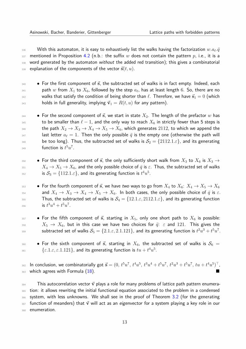
With this automaton, it is easy to exhaustively list the walks having the factorization w.a`.q̄336

mentioned in Proposition 4.2 (n.b.: the suffix w does not contain the pattern p, i.e., it is a337

word generated by the automaton without the added red transition); this gives a combinatorial338

explanation of the components of the vector ~s(t, u).339

• For the first component of ~s, the subtracted set of walks is in fact empty. Indeed, each340

path w from X1 to X6, followed by the step a`, has at least length 6. So, there are no341

walks that satisfy the condition of being shorter than `. Therefore, we have ~s1 = 0 (which342

holds in full generality, implying ~v1 = R(t, u) for any pattern).343

• For the second component of ~s, we start in state X2. The length of the prefactor w has344

to be smaller than `− 1, and the only way to reach X6 in strictly fewer than 5 steps is345

the path X2 → X3 → X4 → X5 → X6, which generates 2112, to which we append the346

last letter a` = 1. Then the only possible q̄ is the empty one (otherwise the path will347

be too long). Thus, the subtracted set of walks is S2 = {2112.1.ε}, and its generating348

function is t5u7.349

• For the third component of ~s, the only sufficiently short walk from X3 to X6 is X3 →350

X4 → X5 → X6, and the only possible choice of q̄ is ε. Thus, the subtracted set of walks351

is S3 = {112.1.ε}, and its generating function is t4u5.352

• For the fourth component of ~s, we have two ways to go from X4 to X6: X4 → X5 → X6353

and X4 → X3 → X4 → X5 → X6. In both cases, the only possible choice of q̄ is ε.354

Thus, the subtracted set of walks is S4 = {12.1.ε, 2112.1.ε}, and its generating function355

is t3u4 + t5u7.356

• For the fifth component of ~s, starting in X5, only one short path to X6 is possible:357

X5 → X6, but in this case we have two choices for q̄: ε and 121. This gives the358

subtracted set of walks S5 = {2.1.ε, 2.1.121}, and its generating function is t2u3 + t5u7.359

• For the sixth component of ~s, starting in X6, the subtracted set of walks is S6 =360

{ε.1.ε, ε.1.121}, and its generating function is tu+ t4u5.361

In conclusion, we combinatorially got ~s = (0, t5u7, t4u5, t3u4 + t5u7, t2u3 + t5u7, tu+ t4u5)>,362

which agrees with Formula (18). �363

This autocorrelation vector ~v plays a role for many problems of lattice path pattern enumera-364

tion: it allows rewriting the initial functional equation associated to the problem in a condensed365

system, with less unknowns. We shall see in the proof of Theorem 3.2 (for the generating366

function of meanders) that ~v will act as an eigenvector for a system playing a key role in our367

enumeration.368

13


4.3 Analytic properties of the kernel: Newton polygons and geometry of branches369

Let us end this section with the proof of an important property of the kernel, the number of370

“small” and “large” roots u(t) of K(t, u) = 0:371

Proposition 4.4 (Small and large roots of the kernel K). All roots u(t) of K(t, u) are either372

small (meaning limt→0 u(t) = 0) or large (meaning limt→0 |u(t)| = ∞). Let dK denote the373

degree of K(t, u) in u, i.e., dK = max{j | [uj]K(t, u) 6= 0}, and let lK denote the lowest374

power of u in the monomials of K, i.e., lK = min{j | [uj]K(t, u) 6= 0}. Then, K has e small375

roots and f large roots, where e = max(0,−lK) and f = max(0, dK)376

Remark 4.5. The nested max /min is needed for the cases where either lK > 0 or dK < 0. An377

example for such a model is S = {−1, 3} and p = [−1,−1], where we have K = 1−u3t−u2t2.378

Proof. Recall that the kernel K is defined as K(t, u) = (1 − tP (u))R(u) + t`ualt(p). Now,379

consider ueK(t, u), which is a polynomial, and draw for each of its monomials tr1ur2 a point380

(r1, r2) in the plane. This gives a set of points P . The Newton polygon6 of K is the boundary381

of the convex hull of P; of particular interest to us are the segments of this polygon that are382

visible when we look from the left: their slope (it is always a rational number) will give the383

exponent of the Puiseux expansions of each root of K. Figure 3 shows schematically all possible384

shapes for the case R(t, u) = 1 (if R(t, u) 6= 1, the possible shapes are more diverse). Each385

segment (in green) which lies below the point (0, e) (they all have a negative slope) gives the386

Puiseux expansion of a set of small roots. Each segment (in red) which lies above the point387

(0, e) (they all have a positive slope) gives the Puiseux expansion of a set of large roots. We388

now focus on the small roots and prove the proposition for them. (The proof for large roots is389

similar and can be obtained from this one by the replacement u 7→ 1u, which corresponds to the390

vertical reflection of the Newton polygon.)391

(0, c)

(1, 0)

(`, c+ h)

(1, c+ d)

(0, c)

(`, c+ h)

(1, c+ d)

(1, 0)

(0,−h)

(1, d− h)

(`, 0)

(1,−c− h)

d < h < d` −c ≤ h ≤ d −c` < h < −c(0, e) = (0, c) (0, e) = (0, c) (0, e) = (0,−h)

Figure 3: Three possibilities for the Newton polygon of the kernel K(t, u). This classificationdepends on the final altitude h of the pattern p, and is exhaustive if R(t, u) = 1. Each point(i, j) corresponds to a monomial tiuj of the numerator of K. The slopes of the convex hullsegments on the left give the Puiseux behaviour at 0 of the small and large roots ui and vj.

6See [34, pp. 106–112] or [51, Chapter 6.3] for a nice presentation of the theory of Newton polygons.

14


If the Newton polygon has no segment of negative slope (the ones drawn in green in392

Figure 3), then K is a polynomial in u (and in t as well) having the constant term 1. Hence,393

K(t, u) = 1 +Q(t, u) where Q(t, u) is a polynomial in t and u with lim(t,u)→(0,0)Q(t, u) = 0.394

This implies that any non large functions u(t) can never compensate the constant term near395

t = 0, and so there are zero small roots and dK large roots, in accordance with e = 0 and396

f = dK .397

If the Newton polygon has at least one such segment of negative slope, then consider one398

of them, denote it by Σ, and let −β/α be its slope. The two endpoints of Σ correspond to399

monomials of ueK(t, u) (some other points of Σ also possibly do). Any two such monomials400

differ by some power of tαu−β. If u ∼ C · tα/β as t → 0, then tαu−β ∼ C−β, which is some401

nonzero constant. Thus, all monomials that correspond to a point of the segment Σ are of402

the same order of magnitude as Puiseux series in t. What about the other monomials? By403

construction of the Newton polygon, their corresponding points must lie above the line containing404

the segment Σ. Hence, such a point can be represented in the form tr1+jur2+k where (r1, r2) ∈ Σ405

and k > −jβ/α. We now use the notation f(t) ≈ g(t) for limt7→0+ f(t)/g(t) = constant. If406

u ≈ tα/β, then one has407

tr1+jur2+k ≈ tr1+j+kα/βur2 .

Since k > −jβ/α, we have j + kα/β > 0 and thus the monomial tr1+jur2+k has a smaller408

order of magnitude than the monomials corresponding to the points of P on the segment Σ,409

like tr1ur2 . The arguments above show that if u ≈ tα/β, then410

ueK(t, u) ≈∑

(r1,r2)∈P∩Σtr1ur2 . (19)411

Now, let (Σ1,Σ2) denote the upper left endpoint of Σ and (Σ3,Σ4) be its lower right412

endpoint. Clearly, the highest power of u in the right-hand side of (19) is uΣ2 and the lowest413

one is uΣ4 . Thus the right-hand side of (19) is a polynomial in u that can be split into uΣ4414

and a polynomial of degree Σ2 − Σ4 which has a nonzero constant term. Hence the number of415

non-trivial solutions equals Σ2 −Σ4. All those solutions are small roots of the kernel. Moreover,416

note that Σ2 − Σ4 is the height of the segment Σ.417

Among all monomials of the form tju−e in K(t, u), let tλu−e be the one where λ is minimal.418

If we draw the Newton polygon of the polynomial ueK(t, u), then it contains the points (0, e)419

and (λ, 0). Assume that the polygonal line we obtain when traversing the boundary of the420

Newton polygon from (0, e) to (λ, 0) consists of line segments Σ1, . . . ,Σr of respective slopes421

−β1/α1, . . . , −βr/αr. Then, the line segment Σj corresponds to a set of small roots of K(t, u)422

each satisfying u(t) ≈ tαj/βj as t→ 0. The number of such roots is equal to the height of Σj,423

which is the difference of the y-coordinates of the two endpoints of Σj . In particular, this implies424

that the number of small roots of K(t, u) is equal to e.425

Using the same reasoning for the line segments (drawn in red in Figure 3) above (0, e), we426

obtain that the number of large roots of the kernel is indeed f .427

Table 2 on the next page gives several examples of plots of these small and large roots.428

Then, equipped with all these notions, we can give the proofs of our main theorems.429

15


p = [1,−2, 1, 1,−2, 1] p = [0, 1, 0, 0, 1, 0] p = [0, 0, 1, 2, 0, 0]

p = [0, 0,−1,−2, 0, 0] p = [−1,−2,−1,−2,−1,−2] p = [−1,−2,−1,−1,−2,−1]

p = [−1,−1, 0,−1,−1, 0] p = [−2,−2, 0,−2,−2, 0] p = [2,−1,−1, 2,−1, 1]

S = {−3, 1}, p = [1, 1] S = {−1, 3}, p = [−1,−1] S = {−1, 1}, p = [1,−1]

Table 2: Several examples that demonstrate the diversity of the behaviour of real branches ofK(t, u) = 0. In all the examples the set of steps is S = {−2,−1, 0, 1, 2} (except for the lastthree examples, where S is indicated explicitly), and the pattern p is as indicated. The kernelK may also have some complex branches (large or small): they are not shown in the figure, butdo play a role in our formulas.

430

431

432

433

434

16


5 Proofs of the generating functions for walks, bridges,435

meanders, and excursions436

In addition to our usual notations for generating functions of different classes of paths, we437

denote by Wα = Wα(t, u) (where 1 ≤ α ≤ `) the bivariate generating function of those walks438

avoiding the pattern p that terminate in state α; similarly Mα = Mα(t, u) for meanders avoiding439

the pattern p that terminate in state α.440

Proof of Theorem 3.1 (Generating function of walks) and proof of Proposition 4.1.441

On the one hand, we have the following vectorial functional equation:442

(W1 · · · W`) = (1 0 · · · 0) + t(W1 · · · W`) A,443

(W1 · · · W`) (I − tA) = (1 0 · · · 0),444

(W1 · · · W`) = (1 0 · · · 0) adj(I − tA)det(I − tA) .

Therefore, the generating functionW (t, u), which is the sum of the generating functionsWα(t, u)445

over all states, is equal to446

W (t, u) = (W1 · · · W`) ~1 = (1 0 · · · 0) adj(I − tA)~1det(I − tA) .447

On the other hand, the generating function for W (t, u) can be obtained using the following448

combinatorial argument which en passant also justifies the introduction of the autocorrelation449

polynomial, as done in the seminal work of Guibas and Odlyzko [45]. We first introduce450

W {p}(t, u), the generating function of the walks over S that end with p and contain no451

other occurrence of p. Then we have W + W {p} = 1 + tPW (if we add a letter from S452

to a p-avoiding walk, then we either obtain another p-avoiding walk, or a walk with a single453

occurrence of p at the end), and Wt`ualt(p) = W {p}R (a walk obtained from a p-avoiding walk454

by appending p at the end, can also be obtained from a walk ending with a single occurrence455

of p at the end by appending the complement of a presuffix of p). Solving this system, we456

obtain W (t, u) = R(t, u)/K(t, u).457

Thus, we got two representations for W (t, u):458

W (t, u) = (1 0 · · · 0) adj(I − tA)~1det(I − tA) = R(t, u)

(1− tP (u))R(t, u) + t|p|ualt(p) . (20)459

In order to see that this is the same representation (that is, the numerators and the denominators460

are equal in both fractions), we notice that det(I − tA) is a polynomial in t of degree ` and461

constant term 1. This is also the case for (1− tP (u))R(t, u) + t`ualt(p), so this allows us to say462

that the two numerators in Formula (20) are actually equal. This gives the proof of Theorem 3.1463

for walks, and also proves Proposition 4.1 on the structure of the kernel.464

We now turn to the consequences of this formula for W (t, u) when one considers bridges.465

17


Proof of Theorem 3.1 (Generating function of bridges).466

In order to find the univariate generating function B(t) for bridges, we need to extract the467

coefficient of [u0] from W (t, u). To this end, we assume that t is a sufficiently small fixed468

number, extract the coefficient of a (univariate) function by means of Cauchy’s integral formula,469

and apply the residue theorem (recall that u1, . . . , ue are the small roots of K(t, u)):470

B(t) = [u0]W (t, u) = 12πi

∫|u|=ε

W (t, u)u

du =e∑i

Resu=ui(t)W (t, u)

u.

By the formula for residues of rational functions, we have471

Resu=ui(t)W (t, u)

u= Resu=ui(t)

R(t, u)u ((1− tP (u))R(t, u) + tùalt(p))472

= R(t, u)ddu

(u ((1− tP (u))R(t, u) + tùalt(p)))

∣∣∣∣∣u=ui(t)

.473

The denominator of this expression is474

−tuP ′(u)R(t, u) + u(1− tP (u))Ru(t, u) + alt(p)tùalt(p)∣∣∣u=ui(t)

. (21)475

Next, we differentiate K(t, ui) = 0 with respect to t and obtain an expression for P ′(ui(t)).476

When we substitute it into (21), we obtain (7).477

We now consider the nonnegativity constraint for the paths.478

Proof of Theorem 3.2 (Generating function of meanders).479

We have the following vectorial functional equation:480

(M1 · · · M`) = (1 0 · · · 0) + t (M1 · · · M`) A− t {u<0}((M1 · · · M`)A

),

or, equivalently,481

(M1 · · · M`)(I − tA) = (1 0 · · · 0)− t {u<0}((M1 · · · M`)A

), (22)482

where {u<0} denotes all the terms in which the power of u is negative.483

The right-hand side of (22) is a vector whose components are power series in t and Laurent484

polynomials in u (of lowest degree ≥ −c). For α = 1, . . . , `, denote the α-th component of485

this vector by Fα = Fα(t, u) (the letter F can be seen as a mnemonic for “forbidden”, as these486

components correspond to the forbidden transitions towards a negative value as exponent of u).487

In summary, one has488

(M1 · · · M`)(I − tA) = (F1 · · · F`). (23)489

We multiply this from the right by (I − tA)−1~1 = (adj(I − tA))~1det(I − tA) . At this point, we denote490

~v = ~v(t, u) := (adj(I − tA))~1, where ~1 is the column vector (1 1 · · · 1)>. This vector ~v is491

the autocorrelation vector we encountered in Proposition 4.2. As a direct consequence of its492

definition, one has493

M(t, u) = (F1 · · · F`)~vK(t, u) . (24)494

18


The following step is the essential part of the vectorial kernel method. Let ui = ui(t) be any495

small root of K(t, u) = det(I − tA). We plug in u = ui(t) into (23). The matrix (I − tA)|u=ui496

is then singular. At this point we observe that ~v|u=ui is an eigenvector of (I − tA)|u=ui497

belonging to the eigenvalue λ = 0. Indeed, ~v|u=ui = (adj((I − tA)|u=ui))~1 is equivalent to498

(I − tA)|u=ui~v|u=ui = det((I − tA)|u=ui)~1, which implies (I − tA)|u=ui~v|u=ui = 0. Moreover,499

due to the structure of A, we have rank((I − tA)|u=ui) = `− 1, therefore, the dimension of500

the characteristic space of λ = 0 is 1, and ~v|u=ui is the unique (up to scaling) eigenvector501

of (I − tA)|u=ui that belongs to λ = 0.502

Thus, if we multiply (23) by ~v|u=ui , the left-hand side vanishes. In other words, the equation503

(F1(t, u), . . . , F`(t, u))~v(t, u) = 0 is satisfied by every small root ui(t) of K(t, u).504

Let505

Φ(t, u) := ue (F1(t, u), . . . , F`(t, u))~v(t, u). (25)506

Note that Φ is a Laurent polynomial, as the Fi’s and ~v are by construction Laurent polynomials507

in u. What is more, since Φ(t, u) = ueM(t, u)K(t, u) by (24) and since M(t, u) is a power508

series in u, Φ(t, u) has no negative powers of u and is thus a polynomial. Now, we know that509

every small root ui(t) of K(t, u) is a root of a polynomial equation510

Φ(t, u) = 0. (26)511

It follows that512

Φ(t, u) = G(t, u)e∏i=1

(u− ui(t)) (27)513

for some G(t, u) which is a formal power series in t and a polynomial in u. We substitute this514

into (24), and obtain the claimed formula515

M(t, u) = G(t, u)ueK(t, u)

e∏i=1

(u− ui(t)).516

If the degree of Φ(t, u) is precisely e, the formula simplifies as G is then just the leading517

term (in u) of Φ(t, u). As we shall show now, this happens if p is a quasimeander (as introduced518

in Definition 3.3).519

Proof of Theorem 3.4 (Generating function of meanders, when p is a quasimeander).520

First, we notice that all the powers of u in R(t, u) are non-negative, and alt(p) ≥ −c. Moreover,521

if alt(p) = −c, the cancellation of terms with u−c in K(t, u) is not possible7. Therefore, the522

lowest power of u in K(t, u) is c, and thus we have e = c by Proposition 4.4.523

Let us return to (22):524

(M1 · · · M`)(I − tA) = (1 0 · · · 0)− t {u<0}((M1 · · · M`)A

). (28)525

7The only exception is the case of p = [−c]. The case of patterns of length 1 is not interesting, so we assumefrom now on that ` ≥ 2. Yet, one can check that our formula is also valid for ` = 1, with some adjustments inthe special case p = [−c].

19


We claim that all the components of the right-hand side, except for the first component,526

are 0. Indeed, if the path arrives at state Xi with i > 1, this means that it accumulated a527

non-empty prefix of p. And since p is a quasimeander, w will always remain (weakly) above the528

x-axis while it accumulates its non-empty prefix.529

Therefore, we have Φ = uc (F1 0 · · · 0)~v, and thus by (15), Φ = ucF1R. Since the530

constant term of F1 is 1, ucF1 is a monic polynomial in u. Therefore, we have531

Φ = R ·c∏i=1

(u− ui).

This yields532

M(t, u) = R(t, u)ucK(t, u)

c∏i=1

(u− ui(t)

)(29)533

as claimed.534

Let us now simplify this formula for excursions, i.e., when u = 0.535

Proof of Theorem 3.4 (Generating function of excursions, when p is a quasimeander).536

The generating function of excursions is given by E(t) = M(t, 0). If alt(p) > −c, we have, as537

u tends to 0, K(t, u) ∼ −tu−cR(t, 0) from (16). If alt(p) = −c, then we have R(t, u) = 1 and538

K(t, u) ∼ −tu−c + t`u−c. In both cases, (11) follows.539

We now handle the next interesting class of patterns leading to generating functions with a540

nice closed form: the case of reversed meanders. Recall that a reversed meander is a lattice541

path whose terminal point has a (strictly) smaller y-coordinate than all other points. Moreover,542

we define a positive meander to be a meander that never returns to the x-axis.543

Proof of Theorem 3.5 (Gen. function of meanders, when p is a reversed meander).544

If p is a reversed meander, then all the terms of R(t, u), except for the monomial 1, contain545

negative powers of u, and we also have alt(p) < 0. Therefore, the highest power of u in K546

is d, and (by Proposition 4.4) the number of large roots of K(t, u) = 0 is d: we denote them as547

above by v1, . . . , vd. The number of small roots can be in general higher than c: as usual, we548

denote it by e, and the roots themselves by u1, . . . , ue.549

We consider the following generalization of the Wiener–Hopf factorization for lattice paths.550

If we split the walk w at its first and at its last left-to-right minimum, we obtain a decomposition551

w = m−.e.m+, where m− is a reversed meander, e is a translate of an excursion, and m+ is a552

translate of a positive meander. One also has the decomposition w = m−.m, where m = e.m+553

is a meander. Notice that these decompositions are unique.554

20


W (t, u)

M(t, u)

M−(t, u)

←−M

+(t, 1/u)

E(t) M+(t, u)

Figure 4: The Wiener–Hopf factorization of a walk: W = M−EM+, a product of a reversed-meander, an excursion, and a positive meander. See e.g. [44] for the importance of thisfactorization for lattice path enumeration. This has further consequences on pattern avoidancewhen one reverses the time.

555

556

557

558

Moreover, since p is a reversed meander, its occurrence cannot overlap the junction of two559

factors. That is, m is p-avoiding if and only if its both factors are p-avoiding, and w is p-avoiding560

if and only if its three factors are p-avoiding. Therefore, we have561

M(t, u) = E(t)M+(t, u), (30)562

and563

W (t, u) = M−(t, u)M(t, u) = M−(t, u)E(t)M+(t, u),564

where W (t, u), M−(t, u), E(t), M+(t, u) are the generating functions of p-avoiding walks,565

reversed meanders, excursions, positive meanders (respectively). This in particular implies566

M(t, u) = W (t, u)M−(t, u) . (31)567

By Theorem 3.1, we have W (t, u) = R(t, u)/K(t, u). In order to find M−(t, u), we use a568

time reversal argument. Namely, we notice that a path is a reversed meander if and only if its569

horizontal reflection (upon translating the initial point to the origin) is a positive meander. The570

precise statement is as follows. Let −S = {−s : s ∈ S}; and for the pattern p = [a1, a2, . . . , a`],571

let ←−p = [−a`, . . . ,−a2,−a1]. Then there is a straightforward bijection between p-avoiding572

reversed meanders with steps from S and ←−p -avoiding positive meanders with steps from −S573

which preserves the length and reflects the altitude. Therefore, we have574

M−(t, u) =←−M+(t, 1/u), (32)575

21


where the arrow means that it is the generating function for←−p -avoiding paths (positive meanders576

in this equation) with the step set −S (rather than p-avoiding with the step set S).577

Refer to the m = e.m+ decomposition above. As we noticed, if the pattern p is a reversed578

meander, then m is p-avoiding if and only if both e and m+ are p-avoiding. The same is true579

if p is a positive meander. Therefore, similarly to Formula (30), M(t, u) = E(t)M+(t, u), we580

also have ←−M(t, u) =←−E (t)←−M+(t, u). Combined with (32), this implies581

M−(t, u) =←−M+(t, 1/u) =←−M(t, 1/u)←−E (t)

. (33)582

Since ←−p is a meander, (9) holds for ←−M(t, u) and we have583

←−M(t, 1/u) = ud

←−R (t, 1/u)←−K (t, 1/u)

d∏j=1

(1u− 1vj(t)

)= udR(t, u)

K(t, u)

d∏j=1

(1u− 1vj(t)

). (34)584

These identities are justified as follows. The equalities ←−R (t, 1/u) = R(t, u) and ←−K (t, 1/u) =585

K(t, u) can be easily derived directly, but also notice that we have W (t, u) = R(t, u)/K(t, u)586

and ←−W (t, 1/u) =←−R (t, 1/u)/←−K (t, 1/u), and W (t, u) =←−W (t, 1/u) from the bijective horizontal587

reflection. Finally, ←−K (t, u) has d many small roots and e many large roots: if ui(t) is a small588

root of K(t, u), then 1/ui(t) is a large root of ←−K (t, u); and if vj(t) is a large root of K(t, u),589

then 1/vj(t) is a small root of ←−K (t, u).590

Similarly, Equation (11) holds for ←−E (t), and we have591

←−E (t) = (−1)d+1

t

d∏j=1

1vj(t)

. (35)592

Notice that the leading term of the polynomial ueK(t, u) is −tud+e and, therefore, one has593

ueK(t, u) = −te∏i=1

(u− ui(t))d∏j=1

(u− vj(t)). (36)594

We now substitute (34) and (35) into (33) and use (36) to obtain595

M−(t, u) = (−1)d+1 t udR(t, u)K(t, u)

d∏j=1

(vj

(1u− 1vj(t)

))(37)596

= −t R(t, u)K(t, u)

d∏j=1

(u− vj(t)) = ueR(t, u)e∏i=1

(u− ui(t)). (38)597

Finally, we substitute this into (31) and obtain598

M(t, u) = W (t, u)M−(t, u) = R(t, u)

K(t, u)1

ueR(t, u)

e∏i=1

(u− ui(t)) = 1ueK(t, u)

e∏i=1

(u− ui(t)). (39)599

600

22


Remark 5.1. It is interesting to notice that though M(t, u), for p being a quasimeander (as601

given in (29)), is similar to M(t, u), for p being a reversed meander (as given in (39)), the latter602

does not contain the factor R(t, u) even if p has a non-trivial autocorrelation.603

Remark 5.2. It is also worth mentioning that if only the terminal point of the pattern p has604

negative y-coordinate, then p is both a quasimeander and a reversed meander, and R = 1.605

Therefore, we have M(t, u) = 1ueK(t, u)

e∏i=1

(u− ui(t)) by both Theorem 3.4 and Theorem 3.5.606

Proof of Theorem 3.5 (Gen. function of excursions, when p is a reversed meander).607

Excursions are given by M(t, 0), so we need to compute D(t) := [u0]ueK(t, u). To this aim,608

first note that as p is a reversed meander (see Definition 3.3), one has the following facts.609

• In all the terms of R(t, u), the powers of u are non-positive.610

• Moreover, if tm1/uγ1 and tm2/uγ2 are two distinct terms in R(t, u) such that 0 ≤ m1 < m2,611

then we have 0 ≤ γ1 < γ2.612

Therefore, we can order the terms of R(t, u) according to the powers of t, and write ueK(t, u)613

as follows:614

ueK(t, u) = ue

(1− t( 1uc

+ · · ·+ ud))(

1 + · · ·+ tm′

uγ′+ tm

uγ

)+ t`ualt(p)

,where tm

uγ(the last term in R(t, u)) corresponds to the longest complement of a presuffix. Now,615

we have the following cases:616

• Case 1: c+ γ > − alt(p). Then e = c+ γ and we have D(t) = −tm+1.617

• Case 2: c+ γ < − alt(p). Then e = − alt(p) and we have D(t) = t`.618

• Case 3: c+γ = − alt(p) and ` 6= m+1. Then e = c+γ = − alt(p) and D(t) = t`−tm+1.619

• Case 4: c+γ = − alt(p) and ` = m+ 1. If ` ≥ 2, then m ≥ 1, and therefore R(t, u) 6= 1.620

Then e = c+ γ′ and D(t) = −tm′+1. As usual, we ignore the degenerate case ` = 1.621

In summary, we get the claim we wanted to prove, namely622

E(t) = M(t, 0) = (−1)e

D(t)

e∏i=1

ui(t), (40)623

where D(t) is either some power of t, or a difference of two powers of t.624

Now that we have proven these closed forms for the generating functions, we can turn to625

the asymptotics of their coefficients.626

23


6 Asymptotics of lattice paths avoiding a given pattern627

The aim of this section is to characterize the asymptotics of the number of paths (walks, bridges,628

meanders, excursions) with steps from S avoiding a given pattern p.629

In order to avoid pathological cases, we now focus on “generic” walks.630

Definition 6.1 (Generic walks). We call a constrained walk model generic if the following five631

properties hold:632

• Property 1. The generating functions B(t),M(t) and E(t) are algebraic, not rational.633

• Property 2. They have a unique dominant singularity, which is algebraic, not a pole.634

• Property 3. The factor G(t, u) in Equation (8) is a polynomial in t.635

• Property 4. Let ρ be the smallest positive real number such that a large branch meets a636

small branch at t = ρ. No large negative branch (i.e., a branch of K(t, u) = 0 such that637

limt→0+ u(t) = −∞) meets a small negative branch at t = ρ.638

• Property 5. The smallest positive root of K(t, 1) is simple.639

These properties are natural and it is easy to analyse the subcases for which they are not holding.640

• For Property 1, it can be the case that the forbidden pattern leads to a degenerate model,641

in the sense that it is no more involving any stack. Thus, we have words generated by a642

regular automaton (hence, the generating functions are rational and the asymptotics are643

well understood). Example: S = {−1, 1} with p = [1,−1] or p = [−1,−1].644

• For Property 2, it is proven in [7] that several dominant singularities appear if and only if645

the gcd of the pairwise differences of the steps is not 1. In this case, the asymptotics are646

obtained via [14, Theorem 8.8]. Moreover, polar singularities are possible, but these are647

easy to handle.648

• For Property 3, it is satisfied in many natural cases (like e.g. in Theorems 3.4 and 3.5)649

and we analyse in the follow-up article [3] what happens otherwise.650

• For Property 4, we conjecture that it always holds. In fact, we have a proof for many651

classes of walks, but some remaining cases are open. Note that it is possible to exhibit652

cases where one small negative root meets a large negative root, at some ρ′ > ρ: this is653

e.g. the case for S = {−2,−1, 0, 1, 2} with p = [0, 1,−2]. Moreover, it is also possible654

that two small negative roots meet at ρ: e.g. for S = {−2, 1} with p = [1,−2, 1,−2].655

• For Property 5, an example of a double root for K is given by S = {−1, 1} and p = [−1, 1]656

(this example corresponds to the very last drawing in Table 2). Double or higher multiplicity657

roots would just create additional subcases (trivial to handle) in the following theorems.658

We observe that the behaviour of real branches of K(t, u) = 0 is much more complicated659

and diverse than that in the Banderier–Flajolet study. To recall, in their case there are always two660

real positive branches (one small branch u1 and one large branch v1) that meet at a singularity661

point (t, u) = (ρ, τ), where u = τ is the only positive number such that P ′(τ) = 0. In contrast,662

in our case we may have additional positive branches – even when the autocorrelation is trivial.663

24


Table 2 from Section 4 illustrates that we always have a small branch and one large branch664

whose shape in general resembles that of u1 ∪ v1 observed for classical paths by Banderier and665

Flajolet. In one sense, the geometry of the branches of K observed for classical paths is now666

perturbed by the pattern avoidance constraint: this perturbation adds new branches. In the667

next section, we introduce the generating function W (t, u, v) where v encodes the number of668

occurrences of the pattern p. One can then play with v like if it would encode a Boltzmann669

weight/Gibbs measure (a typical point of view in statistical mechanics): moving the parameter v670

in a continuous way from 1 to 0 gives a rigorous explanation of this perturbation phenomenon,671

and shows the coherence with the emergence of new branches. More information about these672

branches (and their Puiseux expansions) can be derived from the Newton polygon associated673

with the kernel (see Proposition 4.4 and [34]).674

Lemma 6.2 (Location and nature of the dominant singularity). For any generic model, the675

dominant singularity of B(t) and E(t) is ρ, the smallest real positive number such that a small676

branch meets a large branch at t = ρ. (The branches refer to the roots of K(t, u) = 0, as677

defined in (4)). We call these branches u1 and v1. Additionally, their branching point is a square678

root singularity.679

Proof. Lattice paths avoiding a given pattern can be generated by a pushdown automaton (see680

Figure 1). Accordingly, they can be generated by a context-free grammar, and their generating681

functions thus satisfy a “positive” system of algebraic equations (see [27]). Therefore, the682

asymptotic number of words of length n in such languages is of the form Cρ−nnα. When the683

system is not strongly connected, α is either an integer (if ρ is a pole), either a dyadic number684

(if one has an iterated square root Puiseux singularity at ρ), as proven by Banderier and Drmota685

in [8]. For excursions, one has a strongly connected dependency graph (see Figure 1); the686

dominant singularity ρ (or, possibly, the dominant singularities) thus behaves like a square root,687

as we have generic walks (and not a degenerate case where we face a polar singularity).688

Now, for generic walks, because of the product formula (8) for excursions, one (or several)689

of the small roots have to follow this square root Puiseux behaviour. By Pringsheim’s theorem,690

this has to be at a place 0 < ρ ≤ 1. Note that the Pólya–Fatou–Carlson theorem [26] on pure691

algebraic functions with integer coefficients says that they cannot have radius of convergence 1.692

Therefore, the first crossing between a small and large branch is at 0 < ρ < 1 (i.e., ρ = 1 or693

any other root of t − t`, cannot be the dominant singularity). Now, by Proposition 4.1, the694

geometry of the branches implies that this branching point is at a location where a large branch695

meets a small branch, because if the branching point comes from the intersection of small roots696

only (see the examples 1, 6, 8 in Table 2 for such a case), then their product will be regular. So,697

ρ has to be the smallest real positive number where a small branch meets a large branch.698

When one does not take into account occurrences of a pattern, the generating function of699

bridges is essentially the logarithmic derivative of the generating function of excursions, and700

they have the same radius of convergence (the cycle lemma, the identity B = 1 + Et∂tA,701

Spitzer’s and Sparre Andersen’s formulas are alter egos of this relation, see the paragraph “On702

the relation between bridges and excursions” in [9, Theorem 5]). For walks with a forbidden703

pattern, this simple relation is not holding anymore and there is no apparent equation linking704

the two generating functions. Nevertheless, the numbers en of excursions and bn of bridges705

of length n still satisfy en ≤ bn ≤ nen (this is easily seen by doing the n cyclic shifts of each706

excursion). This implies that E(t) and B(t) have the same radius of convergence.707

25


Equipped with this additional information on the roots and the way they cross, we can708

derive the following asymptotic results. Note that we use the notations Kt(t, u) for (∂tK)(t, u),709

and Kuu(t, u) for (∂2uK)(t, u). We start with the asymptotics of walks on Z with a forbidden710

pattern.711

Theorem 6.3 (Asymptotics of walks on Z). Let ρK be the smallest positive root of K(t, 1).712

For any generic model, the asymptotic number of walks of length n avoiding a pattern p is713

Wn ∼ −ρKKt(ρK , 1)R(ρK , 1)ρ−nK .

Proof. This follows from the partial fraction decomposition of W (t) = R(t,1)K(t,1) , where ρK is a714

simple pole as the model is generic.715

Now, for excursions and bridges, the corresponding generating functions have an algebraic716

dominant singularity; this leads to the following theorems.717

Theorem 6.4 (Asymptotics of excursions). For any generic model, the asymptotic number of718

excursions of length n avoiding a pattern p is719

En ∼ (−1)e−1Y (ρ)G(ρ, 0)D(ρ)

√√√√ Kt(ρ, τ)2πρKuu(ρ, τ) · n

−3/2ρ−n ,

where τ := u1(ρ), Y (t) := u2(t) · · ·ue(t), and D(t) := [u0]ueK(t, u).720

Proof. We use the closed form given in Theorem 3.2. Since the model is generic, the product721G(t,0)D(t) Y (t) is analytic for |t| ≤ ρ. (Caveat: it can be the case that some small branches are not722

analytic for some |t| < ρ, however, their product is then analytic.) Now, for any generic pattern,723

D(t) is either a monomial or of the shape given in Case 3, page 23, but, as ρ < 1 (as shown in724

the course of the proof of Lemma 6.2), one thus has D(ρ) 6= 0. So, the singularity and the725

local behaviour of E(t) is completely determined by the singular behaviour of u1(t). This local726

expansion of u1 is given by a local inversion of K(t, u) at (t, u) = (ρ, τ); this leads to727

u1(t) ∼ τ −

√√√√ 2Kt(ρ, τ)ρKuu(ρ, τ)

√1− t

ρ, as t→ ρ. (41)728

The claim is then reached by singularity analysis (see [42]) on the Puiseux expansion729

E(t) ∼ E(ρ)− (−1)e−1Y (ρ)G(ρ, 0)D(ρ)

√√√√ 2Kt(ρ, τ)ρKuu(ρ, τ)

√1− t

ρ.730

26


Theorem 6.5 (Asymptotics of bridges). For any generic model, the asymptotic number of731

bridges of length n avoiding a pattern p is732

Bn ∼ −R(ρ, τ)τKt(ρ, τ)

√√√√ Kt(ρ, 1)2πρKuu(ρ, 1) · n

−1/2ρ−n .

Proof. We know from Lemma 6.2 that B(t) and E(t) have the same radius of convergence,733

where B(t) is given by Equation (7) from Theorem 3.1. Thus, the singular behaviour of u1(t)734

determines the singularity and the local behaviour of B(t). We have therefore735

B(t) ∼ − R(t, u1(t))Kt(t, u1(t))

u′1(t)u1(t) for t ∼ ρ,

with a denominator Kt which is not 0 for t = ρ. So, plugging the singular expansion of u1 into736

this formula yields the result.737

We now introduce the notion of drift, which plays a role for the asymptotics of meanders.738

Definition 6.6 (Drift of a walk). For any given set of steps S and forbidden pattern p, the739

drift is the quantity740

δ := limn→∞

average final altitude of walks on Z of length nn

.741

Thus δ > 0, δ < 0, or δ = 0 correspond to the fact that almost all the walks of length n on Z742

have a final altitude of order which is either +Θ(n), −Θ(n), or o(n), respectively. One says743

that these walks (and the corresponding meanders/excursions/bridges) have a positive, negative744

or zero drift, respectively.745

As usual, the drift is not playing a role for the asymptotics of excursions and bridges. Indeed,746

the constraint to force the walk to end at altitude zero is there “killing" the drift. This is best747

seen by a “time reversal” argument: under this transformation, a bridge stays a bridge (which748

then avoids the reverse forbidden pattern), one thus gets the same generating function (note749

that K(t, u) then becomes K(t, 1/u)); therefore, the asymptotics have to be independent of750

the drift. A similar reasoning holds for excursions. Now, the next theorem shows how the drift751

does play a role for the asymptotics of meanders. For meanders with negative or zero drift,752

the quantity ρ from Lemma 6.2 is also the radius of convergence of M(t). For meanders with753

positive drift, the radius of convergence of M(t) is the dominant pole of 1/K(t, 1).754

27


Theorem 6.7 (Asymptotics of meanders). Assume that the model is generic. Let ρ, ρK , and τ755

be defined like in the previous theorems. We have one of the following three cases:756

• If τ = 1 and ρK = ρ, then we are in the “zero drift” case.757

• If τ > 1 and u1(ρK) = 1 and all large roots v satisfy v(t) 6= 1 for ρK < t < ρ, then we758

are in the “negative drift” case.759

• If either τ < 1, or τ = 1 but ρK < ρ, or τ > 1 but some large root v satisfies v(ρK) = 1,760

then we are in the “positive drift” case.761

Then the asymptotics of the coefficients of the meander generating function762

M(t) = (1− u1(t))Y (t)G(t, 1)K(t, 1) with Y (t) :=

c∏i=2

(1− ui(t))763

is given by764

Mn ∼ G(ρ, 1)Y (ρ)√

2πρKt(ρ, 1)Kuu(ρ, 1) · n

−1/2ρ−n (“zero drift”),765

Mn ∼ −G(ρ, 1)Y (ρ)K(ρ, 1)

√√√√ ρKt(ρ, τ)2πKuu(ρ, τ) · n

−3/2ρ−n (“negative drift”),766

Mn ∼ −(1− u1(ρK))Y (ρK)G(ρK , 1)

ρKKt(ρK , 1) · ρ−nK (“positive drift”).767

Proof. Before we begin the case analysis, let us mention some preliminary facts. The line u = 1768

intersects the curve shaped by u1 ∪ v1 at some point (t0, 1) (see Figure 5). Notice that the769

right-most point of this curve is (ρ, τ). Thus t0 ≤ ρ, where equality holds if and only if τ = 1.770

Moreover, observe that K(t0, 1) = 0 and thus ρK ≤ ρ, where equality can only hold if τ = 1.771

This last fact comes as no surprise, as the growth rate of all walks on Z is larger or equal to the772

growth rate of meanders, which are a subset of walks restricted on N. It also tells us that the773

three cases listed in the assertion cover all possibilities that may appear for generic walks.774

Zero drift case: To prove the assertion, observe that the dominant singularity of the775

generating function M(t) = (1− u1(t))Y (t)G(t, 1)/K(t, 1) is at ρK = ρ and it originates from776

a simple zero in the denominator K(t, u) and from u1. The singular expansion of u1(t) at ρ777

(see Formula (41)) gives778

M(t) ∼ G(ρ, 1)Y (ρ)ρKt(ρ, 1)

√√√√2ρKt(ρ, 1)Kuu(ρ, 1)

(1− t

ρ

)−1/2

= G(ρ, 1)Y (ρ)√

2√ρKt(ρ, 1)Kuu(ρ, 1)

(1− t

ρ

)−1/2

.779

Negative drift case: We have τ > 1 and thus, by the preliminary facts listed in the first780

paragraph, ρK < ρ. So, there is a simple zero of K(t, 1) at ρK , but this is cancelled, as781

28


S = {−1, 1}p = [1,−1, 1,−1]τ = 1 (zero drift)

S = {−2, 1}p = [1,−2, 1,−2]

τ > 1 (negative drift)

S = {−1, 2}p = [2,−1, 2,−1]

τ < 1 (positive drift)

Figure 5: For the asymptotics of meanders, the key is to compare the location of the singularity ρ(the branching point of u1, v1) with the zeroes of K(t, 1), and the values t such that ui(t) = 1.

800

801

u1(ρK) = 1. Now, u1 has a square-root type singularity at ρ, thus singularity analysis gives the782

last claim of the theorem, via the following Puiseux expansion at the dominant singularity ρ783

M(t) ∼M(ρ) + G(ρ, 1)Y (ρ)K(ρ, 1)

√√√√2ρKt(ρ, τ)Kuu(ρ, τ)

√1− t

ρ.784

Note that there may be a second zero of K(t, 1), say ρ2, which is smaller than ρ (and larger785

than ρK). This means there is a small root u2(t) (large roots are excluded in the negative drift786

case) of the kernel satisfying u2(ρ2) = 1. As Y (t) contains the factor 1 − u2(t), this zero is787

cancelled. In case the root ρ2 is a multiple zero of K(t, 1), say of order ω, then there must be788

ω roots u2(t), . . . , uω+1(t) which meet at t = ρ2, causing a singularity of order ω. But then789

again the factors 1− ui(t), i = 2, . . . , ω, in Y (t) cancel the pole. The same happens if further790

zeros of K(t, 1) appear before ρ. Hence we conclude that the dominant singularity of M(t) is791

at ρ and originates from the dominant singularity of u1(t).792

Positive drift case: Here we have several subcases. Assume first that τ < 1 or τ = 1 and793

ρK < ρ. In fact, by the preliminary facts from the first paragraph, we know that we have in794

both cases ρK < ρ, and hence the generating function has the dominant singularity ρK which795

comes from the kernel only and is a simple pole. This implies796

M(t) ∼ (1− u1(ρK))Y (ρK)G(ρK , 1)ρKKt(ρK , 1)

11− t/ρK

.

If τ > 1, like in the negative drift case, and some large root v satisfies v(ρK) = 1, then there is797

no more a cancellation of the zero of K(t, 1) by one of the factors in Y (t). Thus M(t) has a798

simple pole at ρK and we get the same expression as in the other subcases.799

These asymptotics also allow us to get results on limit laws, as presented in the next section.802

29


7 Limit law for the number of occurrences of a pattern803

Our approach also allows us to count the number of occurrences of a pattern in paths. As usual,804

an occurrence of p in w is any substring of w that coincides with p, and when we count them805

we do not require that the occurrences will be disjoint. For example, the number of occurrences806

of 11 in 1111 is 3. One has807

Theorem 7.1 (Trivariate generating function for walks). The generating function of the number808

of occurrences of the pattern p in walks on Z is809

W (t, u, v) = 11− tP (u)− tùalt(p)(v − 1)/(1− (v − 1)(R(t, u)− 1)) . (42)810

Proof. We give two proofs, each of them having its own interest. Both of them are of wider811

applicability, see [42, p. 60 and p. 212].812

First proof, via symbolic inclusion-exclusion. Define a cluster as a sequence of repetitions of813

the pattern p (possibly overlapping), where each occurrence of p is marked by the variable v, so814

the set C of clusters is given by C = vp Seq(v(Q̄ − ε)), where Q̄ − ε is the set of nonempty815

complements of presuffixes of p (the generating function of which is R(t, u)−1, see Formula (3)).816

Obviously, W (t, u, v + 1) = Seq(S + C). This directly gives (42).817

Second proof, via a system/adding a jump approach. Let W ≡ W (t, u, v) and Wp ≡818

Wp(t, u, v) be the generating functions of all words and, respectively, of words ending with p,819

where v counts the number of occurrences of p. We show the following two identities:820

1 +WtP = W −Wp + v−1Wp , (43)821

Wtùalt(p) = v−1WpR− (R− 1)Wp . (44)822

To show (43), take a word and add a letter to it. If the resulting word does not end with p, it is823

counted by W −Wp; if it does, it is counted by v−1Wp. To show (44), take a word w with i824

occurrences of p and consider the contribution of w.p to both sides of the equation. Adding825

the pattern p to w creates a number j of extra occurrences of p. The path w.p can be written826

in j ways as w′r, where w′ ends with p and r is an autocorrelation factor, or j − 1 ways if we827

impose that r 6= ε. The word w.p therefore contributes with a factor vi to Wtùalt(p), with828

a factor vi+1 + · · ·+ vi+j to WpR and with a factor vi+1 + · · ·+ vi+j−1 to Wp(R − 1). The829

formula (42) follows.830

In order to get the formula for meanders, we reconsider the associated automaton and its831

adjacency matrix A: we add a mark v to the transition which would lead to an occurrence of p832

(see Figure 6). As833

W (t, u, v) = (1 0 · · · 0) adj(I − tA)~1det(I − tA) , (45)834

the above theorem has the consequence that835

det(I − tA) = (1− v)((1− tP (u))R(t, u) + tùalt(p)) + v(1− tP (u)). (46)836

This last equality follows from the fact that the denominators of the rational functions (in Q(t))837

in (45) and (42) are in fact the same irreducible polynomial of degree ` in t.838

30


[1,2,-1,1][1,2,-1][1,2][1]ε

X1 X2 X3 X41 2 −1 1

−1, 2 1−1 21

X5

12 −1−1, 2

u−1 + u2

u−1

u2

u−1 + u2

u−1

u

u

u

u−1

u2

u

A = u

u2v

Figure 6: Pushdown automaton and its associated adjacency matrix A. The automatongenerates walks with the set of steps S = {−1, 1, 2}, and marks each occurrence of the patternp = [1, 2,−1, 1, 2]. In dashed red we marked the arrow from the last state X` labelled by a`,the last letter of the pattern. Giving a weight v to this transition leads to enumerative formulasinvolving det(I − tA) as given in Equation (46).

839

840

841

842

843

Accordingly, the trivariate kernel is thus defined as K(t, u, v) := det(I − tA). Note that844

for v = 0 we get the kernel from the avoidance case (see equation (4)), and for v = 1 we get845

1− tP (which is, as expected, the kernel from [9]). The formulas for the trivariate generating846

functions of bridges, meanders, and excursions are thus like in Theorems 3.1 and 3.2, where847

the ui’s are now the small roots of the trivariate kernel. This allows us to prove a universal848

asymptotic behaviour, an instance of what Flajolet and Sedgewick pleasantly called Borges’s849

theorem (we comment more on it in the conclusion).850

Theorem 7.2 (“Borges’s theorem”: Gaussian limit laws for occurrences). Let Xn be the random851

variable which counts the number of occurrences of a pattern in a generic walk, bridge, meander,852

excursion model. Then Xn has a Gaussian limiting distribution with E[Xn] = µn+O(1) and853

Var[Xn] = σ2n+O(1) for some constants µ > 0 and σ2 ≥ 0:854

1√n

(Xn − E[Xn])→ N (0, σ2).855

Proof. All these combinatorial structures are generated by context-free grammars [7, 36, 56, 61].856

Accordingly, their generating functions satisfy a positive algebraic systems. Thus, it leads to857

Gaussian limit laws, as proven in [8, Theorem 9]: it comes from following the dependencies858

in the graph associated with the system, and applying Hwang’s quasi-power theorem to each859

component. To apply it, a positive variance condition has to be checked: this is done via860

the trivariate version of the formulas of Theorems 3.1 and 3.2, with the additional variable v861

counting the number of occurrences of the pattern.862

31


8 Examples, pushdown automata863

Directed lattice paths can be generated by context-free grammars [56], and it is well-known864

that context-free grammars and pushdown automata/counter automata are related (see the865

“Cinderella Book” [48, Sections 6.3, 6.4, and 8.5.4]). We want here to promote the idea that866

pushdown automata are a powerful approach for lattice path enumeration. Conversely, any867

pushdown automaton enumeration can be seen as a lattice path problem (the stack encodes the868

altitude of the path), this allows us to solve it via our vectorial kernel method. This is due to869

the fact that pushdown automata have mainly two notions of acceptance:870

• acceptance by empty stack, this corresponds to the generation of excursions;871

• acceptance by final state (whatever the value of the stack is), this corresponds to the872

generation of meanders.873

Let us now illustrate our method by diverse examples.874

Example 8.1 (Forbidden patterns). We start with our initial problem of lattice paths with875

forbidden patterns. Our theorems rediscover, in a uniform way, numerous results by different876

authors obtained in the last years by different methods. We present some of them in Table 3. �877

steps, pattern of length `, model generating function OEIS reference8

S = {−1, 0, 1}p = [1, 0, . . . , 0,−1]Bridges

1√1− 2t− 3t2 + 2t` − 2t`+1 + t2`

` = 2: A051286(confirms a conjecture therein onWhitney numbers; see also [21])

S = {−1, 0, 1}p = [1, 0, . . . , 0,−1]Meanders

1−3t+t`−√

1−2t−3t2+2t`−2t`+1+t2`2t(1−3t+t`)

` = 2: A091964(RNA folding, see [47])

S = {−1, 0, 1}p = [1, 0, . . . , 0,−1]Excursions

1−t+t`−√

1−2t−3t2+2t`−2t`+1+t2`2t2

` = 2: A004148 [50]` = 3: A114584 [58, 82]

S = {1,−1}p = [1,−1, 1,−1, . . . , 1]Excursions

1−t`+1−√

1−4t2+2t`+1+4t`+3−3t2`+2

2t2(1−t`−1)` = 3: ≈ A001006(Motzkin numbers [73, 81])

S = {1,−1}p = [1,−1, 1,−1, . . . ,−1]Excursions

1−t`+2−√

1−4t2+6t`+2−4t2`+2+t2`+4

2t2(1−t`)

` = 4: A078481(irreducible stacksortable permutations, [15,59])

878

Table 3: A few examples in which our theorems produce sequences listed in the On-LineEncyclopedia of Integer Sequences. They uniformly rediscover results from several earlier works,often related to Dyck/Motzkin paths, and in certain cases also confirm conjectures.

879

880

881

Next we now give several examples of a wide variety of questions on lattice paths, that can882

also be tackled with our approach. In some cases, we omit the closed forms: they are just a883

direct application of our approach, once the adjacency matrix A is known. Some pushdown884

automata lead to a system for which an additional argument is needed to identify the factor G885

in Theorem 3.2; we study this situation in more detail in [3].886

8Such references are links to the webpage dedicated to the corresponding sequence in the On-Line Encyclopediaof Integer Sequences (OEIS), https://oeis.org.

32

https://oeis.org/A051286






https://oeis.org


Example 8.2 (Motzkin paths without peaks and valleys).887

X0

X− X+

0

0

01

1

1

−1

−1 −1

The automaton on the left allows us to count Motzkin pathsby marking each peak (i.e., the pattern [1,−1]) and eachvalley (i.e., the pattern [−1, 1]). Forbidding the transitionsshown by red dashed lines, we get the automaton forMotzkin paths without peaks and valleys. Then the kernelis K(t, u) = t3u+t2u−tu2−tu−t+u

u, and it has one small root

u0(t) = 1−t+t2+t3−√

(1−t4)(1−2t−t2)2t . The degree of Φ (as in

Equation 25) is equal to the number of small roots of K,and taking care of the leading term (in u) of Φ we obtain

M(t, u) = 1− t2

1− tu0(t)u− u0(t)uK(t, u) .

888

Setting u = 1, we get the generating function for meanders889

M(t) = M(t, 1) = −(1 + t)(1− 2t− t2)−

√(1− t4)(1− 2t− t2)

2t2(1− 2t− t2) =

√1−t4

1−2t−t2 − t− 12t2 ,

which corresponds to the sequence A308435.890

Setting u = 0, we get the generating function for excursions891

E(t) = M(t, 0) =(1 + t)(1− t)2 −

√(1− t4)(1− 2t− t2)

2t2 ,

which corresponds to the sequence A004149. �892

Example 8.3 (Basketball with alternation of team scoring).893

X− X+

1, 2

−1,−2

X0

1, 2−1,−2

In the pre-1980s basketball rules, each team could score 1or 2 points at once. Zeilberger and other authors [4,11,23]therefore considered the model of (old-time) basketballexcursions, where the step set is S = {2, 1,−1,−2}. Ifwe now add the constraint that each team cannot scoretwice in a row, this gives the automaton presented on theleft. It yields the bivariate generating function

894

M(t, u) = (1 + tu+ tu2) u− (tC(t2))2

u− (t(u+ 1))2 , where C(t) = 1−√

1− 4t2t .895

896

This yields M(t, 1) = C(t2)√

1 + 2t1− 2t =

√1+2t1−2t − 1− 2t

2t2 and E(t) = M(t, 0) = C2(t2),897

which correspond to the sequences A001405 and A126120. �898

33






Example 8.4 (Walks/meanders/excursions of bounded height).899

If one consider meanders of altitude bounded by h, they are easily generated by an automaton900

with h states. In fact, the reader now familiar with our approach will realize that a pushdown901

automaton with just one state is already enough: the kernel equation will encode the boundedness902

by h and the positivity constraint! See [7, 12, 23] for further considerations on the closed forms903

obtained. This bypasses the quickly intractable resolution of a system h× h. �904

Example 8.5 (Partially directed self-avoiding walks).905

We can link some self-avoiding walks and pattern avoiding lattice paths. In fact, the enumeration906

and the asymptotics of self-avoiding walks in Z2 is one of the famous open problems of907

combinatorics and probability theory. As it is classical for intractable problems, many natural908

subclasses have been introduced, and solved. E.g., partially directed self-avoiding walks with an909

added constraint of living in a half-plane or a strip [6]: they have three kinds of steps, say n, e,910

and s, and the self-avoiding condition means that factors ns and sn are disallowed. Consider the911

following three models:912

• in the first model, the half-plane is the one over the line x = 0; the heights of the steps913

are alt(n) = 1, alt(e) = 0 and alt(s) = −1;914

• in the second model, the half-plane is the one over the line x = y; the heights are915

alt(n) = 1, alt(e) = −1 and alt(s) = −1;916

• in the third model, the half-plane is the one over the line x = −y; the heights are917

alt(n) = 1, alt(e) = 1 and alt(s) = −1.918

These models are illustrated in Figure 7. Each of them leads to an algebraic generating function,919

expressible via our method as a closed form involving the roots of the kernel. �920

Figure 7: Some models of self-avoiding walks are encoded by partially directed lattice pathsavoiding a pattern (see [6]).

921

922

34


Example 8.6 (Motzkin paths with horizontal steps only at even/odd altitude).923

If one wants to allow some specific set of steps depending on the altitude modulo some period, the924

vectorial kernel method will do the job! Let us illustrate this with Motzkin paths (S = {1, 0,−1})925

with horizontal steps only at even altitude.926

XE XO

−1, 1

−1, 1

0

XE XO

−1, 1

−1, 1

0

This pushdown automaton has two states, the first one cor-responds to even altitudes, the second one to odd altitudes.By design, it is clear that it generates Motzkin walks withhorizontal steps only at even altitude. Our vectorial kernelmethod then captures the additional constraint of the positivityof the stack, and thus gives the generating function for me-anders (A307557) and excursions (A090344). En passant, letus mention that excursions are given by a pleasant continuedfraction (see e.g. [41] for a nice survey):

E(t) =1

1− t−t2

1−t2

1− t−t2

1−t2

1− . . .

.

If we want to enumerate Motzkin paths with horizontal stepsonly at odd altitude, we adjust the automaton as shown onthe left, and obtain the sequences A327421 (for meanders) andA090345 (for excursions), see e.g. [18, 32].

927

�928

Example 8.7 (Duchon’s club without lonely visitors).929

2,−3X1

The terminology of Duchon’s club was introduced in [9] as a playful referenceto the nice article [36]. As some readers may wonder, we have to add thatit is in no way an allusion to some fancy habit of our highly honourableand very respectable colleague Philippe Duchon! Here is the story. In theearly evening, the club opens empty, and then, during the full night, peopleare entering in couples and leaving in groups of three people. Finally, theclub closes empty at the end of the night. For sure, you do not want to bealone in such a club! What is the number of possible scenarios? These areexcursions with step set S = {2,−3} and never going to altitude 1. Thisenumeration is encoded by a single state automaton, and the kernel equationthen fully handles all the constraints. This leads to the sequences A327422(for meanders) and A327423 (for excursions).

930

�931

35








Example 8.8 (Counting/avoiding humps and peaks in Motzkin paths).932

Consider Motzkin walks: S = {−1, 0, 1}. A peak is the pattern [1,−1]. A hump is an occurrence933

of the pattern [1, 0∗,−1], that is, 1 followed by a (possibly empty) sequence of 0s, followed934

by −1. Humps were considered e.g. in [35, 60,72]. We first consider the generating function of935

walks counting the number of humps, similarly to our approach from Section 7.936

X1 X2 X3

1 0

0,−1

−1

−1 0

1

1

The transition which was forbidden in thepattern avoidance setting is here representedwith a variable v in the adjacency matrix A.This yields the trivariate generating functionwith respect to length (t), final altitude (u),and number of occurrences of humps (v).In particular, this leads to a Gaussian distri-bution, see Borges’s Theorem 7.2.

937

Note that, upon a straightforward modification, the above automaton works not only for938

the Motzkin walks, but also for any set of steps S ⊇ {−1, 0, 1}. Furthermore, this offers more939

multivariate statistics “for free”. E.g., we can assign the weight v to X3−1−→ X1 and the weight940

vw to the transition X2−1−→ X1: this will count humps by v, and peaks by w. Our approach941

then gives the following closed form for the corresponding quadrivariate generating function942

F (t, u, v, w) =√

∆ + (1− w) vt3 + (vw − 2u− 2) t2 + (2u+ 2) t− 12t(uv (w − 1) t3 + (−uvw + u2 + 2u+ 1) t2 − (1 + u)2 t+ u

)943

∆ =((w − 1) vt3 − t2vw + 1

) ((w − 1) vt3 + (−vw + 4) t2 − 4 t+ 1

).944

Now, the generating function of excursions with an even number of humps is945

F (t, 0, v, w)/2 + F (t, 0,−v, w)/2.946

If one additionally wants, say, an odd number of peaks, then the generating function is947

12

(F (t, 0, v, w) + F (t, 0,−v, w)

2 − F (t, 0, v,−w) + F (t, 0,−v,−w)2

).948

Similar manipulations for different combinations of avoidance and parity constraints for peaks949

and humps lead to results summarized in the following table (we give the OEIS entries for the950

corresponding sequences of meanders and excursions).951

even numberof humps

odd numberof humps

any numberof humps

no peaks M: A325917E: A325918

M: A325919E: A325920

M: A091964E: A004148

even numberof peaks

M: A325921E: A325922

M: A325923E: A325924

M: A307575E: A307576

odd numberof peaks

M: A325925E: A325926

M: A325927E: A325928

M: A307577E: A307578

any numberof peaks

M: A307555E: A307564

M: A307572E: A307573

M: A005773E: A001006

952

We omit the case of walks with no hump, as it would lead to trivial rational functions. �953

36


























In fact, there are several thousand sequences related to directed lattice paths in the On-Line954

Encyclopedia of Integer Sequences, and several hundreds of them can be generated and analysed955

via the method presented in this article. Let us give a few examples illustrating different types956

of set of steps and constraints:957

• Dyck excursions with up steps colored in two colors (blue and red, denoted UB and UR),958

and avoiding the pattern UBUR (A006013, which also enumerates many other objects!),959

• Motzkin excursions avoiding UD, UU and DD (see A023432 and [31]),960

• Schröder bridges (also called Delannoy paths) with k occurrences of DD that cross y = 0961

(see A110121 and [13,80]),962

• excursions from (0, 0) to (3n, 0) that use steps u = (2, 1), U = (1, 2), and D = (1,−1),963

and have k peaks uD or UD (see A108425 and [30]),964

• Łukasiewicz paths with k U-steps that start at an even level (see A091894 and [16,20]).965

Moreover, there is a vast world of combinatorial models that can be encoded by pushdown966

automata and, therefore, fall under the scope of the vectorial kernel method, for example:967

• patterns in permutations (see e.g. A105633, and [67,70]),968

• patterns in trees and lambda terms (see e.g. A114997, A105633, and [19,29,74]),969

• patterns in RNA structures (see e.g. A103140 and [47,50]),970

• enumeration in Tamari-like posets (see e.g. A007477 and [5, 17]),971

• a mathematical model for bobbin lace (see A291083 and [49]).972

We also list 200 other examples at the webpage https://lipn.fr/~cb/KernelMethod/,973

where we maintain a list of OEIS references and publications focusing on objects which can974

be handled by the vectorial kernel method. Moreover, many of these OEIS entries contain975

conjectures on the recurrence satisfied by the sequence, or its asymptotics, or the algebraic976

equation satisfied by the corresponding generating function: in numerous cases such conjectures977

can directly be solved by the vectorial kernel method and basic computer algebra manipulations.978

For some of these examples, it is possible to tackle the problem by using some ad hoc979

decompositions, bijections with trees, or some variation of a classical kernel method [28, 37,43,980

46,54,55,63–65,68,71,75,79]. Some examples require to mark several patterns at once, or to981

take a diagonal of our multivariate generating function (e.g. when the number of occurrences of982

a given pattern is required to be proportional to the length n, or to the number of occurrences of983

another pattern), etc. The method is really flexible and allows playing with variants of patterns,984

step sets, colors, weights, values of the stack, constraints modulo 2, 3, . . . an endless game!985

We emphasize that the full approach is automatable (sic ?), so all such studies can now986

morally be considered as computationally solved by our vectorial kernel method, with some987

subtleties which will be presented in the follow-up article [3]. Thus, in a style dear to the heart988

of Shalosh B. Ekhad and Philippe Flajolet, the vectorial kernel method can be considered as a989

method to automatically prove enumerative and asymptotic results for pattern occurrences in990

structures given by an algebraic system of functional equations.991

37












https://lipn.fr/~cb/KernelMethod/


9 Conclusion992

In this article, we presented a unifying way which gives the generating functions and asymptotics993

of all families of lattice paths with a forbidden pattern, and we proved that the number of994

occurrences of a given pattern is normally distributed. The same techniques would, for instance,995

allow us to do the asymptotics of walks having exactly m occurrences of a given pattern, or to996

consider patterns which are no longer a word but a regular expression.997

It is also nice that our approach gives a method to solve in an efficient way the question of998

the enumeration and asymptotics of words generated by a pushdown automaton (or words999

belonging to the intersection of an algebraic language and a rational language). What is more,1000

it is possible to use our functional equation approach to analyse the intersection of two algebraic1001

languages. Note that testing whether this intersection is empty is known to be an undecidable1002

problem, even for deterministic context-free grammars (see e.g. [48]), so we cannot expect1003

too much from a generic method in this case. However, we can specify the type of system of1004

functional equations that we get: indeed, this problem is related to automata with two stacks,1005

which, in turn, are known to have the same power as Turing machines; the evolution of these1006

two stacks corresponds to lattice paths in the quarter plane (with steps of arbitrary length), the1007

complexity of the problem is reflected by the fact that one can then get generating functions1008

which are no more algebraic, D-finite, or differentially-algebraic, and we do not expect some1009

nice universal enumerative closed-form results here but a wider zoo of formulas. On the other1010

hand, some universal asymptotic behaviour is expected; it is highly believable that all these1011

cases will be new instances of what Flajolet and Sedgewick called Borges’s Theorem: Any1012

pattern which is not forbidden by design will appear a linear number of times in large enough1013

structures, with Gaussian fluctuations.1014

For sure, it is more a metatheorem, a natural credo, and the claim should be established1015

rigorously in each case. Naturally, may it be with tools of probability theory or of analytic1016

combinatorics, there is always some technical conditions to check to ensure this claim. In this1017

article, our closed form expressions for the generating functions were one of the keys, together1018

with the universal behaviour of the small roots. This allowed us to prove this Gaussian behaviour1019

for the number of occurrences of any given pattern. Year after year, this claim is established for1020

more and more combinatorial structures (it was done for patterns in Markov chains, trees, maps,1021

permutations, context-free grammars, and now... lattice paths!).1022

Let us conclude with the passage of Flajolet and Sedgewick [42, p. 61] which explains where1023

the concept of Borges’s Theorem comes from:1024

This property is sometimes called “Borges’s Theorem” as a tribute to the famous Argentinianwriter Jorge Luis Borges (1899-1986) who, in his short story “The Library of Babel”, describesa library so huge as to contain:

“Everything: the minutely detailed history of the future, the archangels’ autobiographies,the faithful catalogues of the Library, thousands and thousands of false catalogues, thedemonstration of the fallacy of those catalogues, the demonstration of the fallacy ofthe true catalogue, the Gnostic gospel of Basilides, the commentary on that gospel,the commentary on the commentary on that gospel, the true story of your death, thetranslation of every book in all languages, the interpolations of every book in all books.”

1025

38


Acknowledgements: We thank the organizers and referees of the conferences AofA 20181026

and LATA 2018, where we presented some aspects of this work (see [1, 2]). This work was1027

supported by the Austrian Science Fund (FWF), in the framework of the Special Research1028

Program Algorithmic and Enumerative Combinatorics (grant SFB F50-03) and of the project1029

Analytic Combinatorics: Digits, Automata and Trees (grant P 28466-N35).1030

References1031

[1] Andrei Asinowski, Axel Bacher, Cyril Banderier, and Bernhard Gittenberger. Analytic1032

combinatorics of lattice paths with forbidden patterns: asymptotic aspects. In 29th1033

International Conference on Probabilistic, Combinatorial and Asymptotic Methods for the1034

Analysis of Algorithms (AofA 2018), volume 110 of Leibniz International Proceedings in1035

Informatics (LIPIcs), pages 10.1–10.13, 2018.1036

[2] Andrei Asinowski, Axel Bacher, Cyril Banderier, and Bernhard Gittenberger. Analytic1037

combinatorics of lattice paths with forbidden patterns: enumerative aspects. In Language1038

and Automata Theory and Applications. LATA 2018, volume 10782 of Lecture Notes in1039

Computer Science, pages 195–206. Springer, 2018.1040

[3] Andrei Asinowski, Axel Bacher, Cyril Banderier, and Bernhard Gittenberger. Pushdown1041

automata, the vectorial kernel method, and underdetermined functional equations. In1042

preparation, 2019.1043

[4] Arvind Ayyer and Doron Zeilberger. The number of [old-time] basketball games with final1044

score n : n where the home team was never losing but also never ahead by more than w1045

points. Electron. J. Combin., 14(1):Article R19, 8 pp., 2007.1046

[5] Axel Bacher, Antonio Bernini, Luca Ferrari, Benjamin Gunby, Renzo Pinzani, and Julian1047

West. The Dyck pattern poset. Discrete Math., 321:12–23, 2014.1048

[6] Axel Bacher and Mireille Bousquet-Mélou. Weakly directed self-avoiding walks. Journal of1049

Combinatorial Theory, Series A, 118(8):2365–2391, 2011.1050

[7] Cyril Banderier. Combinatoire analytique des chemins et des cartes . PhD thesis, Université1051

Paris VI, 2001.1052

[8] Cyril Banderier and Michael Drmota. Formulae and asymptotics for coefficients of algebraic1053

functions. Combinatorics, Probability and Computing, 24(1):1–53, 2015.1054

[9] Cyril Banderier and Philippe Flajolet. Basic analytic combinatorics of directed lattice paths.1055

Theoretical Computer Science, 281(1-2):37–80, 2002.1056

39

https://lipn.univ-paris13.fr/~banderier/Papers/aofa2018_patterns.pdf



http://dx.doi.org/10.1007/978-3-319-77313-1_15

http://dx.doi.org/10.1007/978-3-319-77313-1_15

http://dx.doi.org/10.1007/978-3-319-77313-1_15

http://www.combinatorics.org/ojs/index.php/eljc/article/view/v14i1r19/pdf





https://doi.org/10.1016/j.disc.2013.12.011

https://www.sciencedirect.com/science/article/pii/S0097316511001002/pdf

https://lipn.univ-paris13.fr/~banderier/Papers/these.pdf

http://lipn.univ-paris13.fr/~banderier/Papers/Alg.pdf





[10] Cyril Banderier and Bernhard Gittenberger. Analytic combinatorics of lattice paths: enumer-1057

ation and asymptotics for the area. Discrete Math. Theor. Comput. Sci. Proc., AG:345–355,1058

2006.1059

[11] Cyril Banderier, Christian Krattenthaler, Alan Krinik, Dmitry Kruchinin, Vladimir Kru-1060

chinin, David Nguyen, and Michael Wallner. Explicit formulas for enumeration of lattice1061

paths: basketball and the kernel method. In Lattice paths combinatorics and applications,1062

Developments in Mathematics Series, Vol. 58, pages 78–118. Springer, 2019.1063

[12] Cyril Banderier and Pierre Nicodème. Bounded discrete walks. Discrete Math. Theor.1064

Comput. Sci., AM:35–48, 2010.1065

[13] Cyril Banderier and Sylviane Schwer. Why Delannoy numbers? J. Statist. Plann. Inference,1066

135(1):40–54, 2005.1067

[14] Cyril Banderier and Michael Wallner. The kernel method for lattice paths below a rational1068

slope. In Lattice paths combinatorics and applications, Developments in Mathematics1069

Series, Vol. 58, pages 119–154. Springer, 2019.1070

[15] Jean-Luc Baril. Avoiding patterns in irreducible permutations. Discrete Math. Theor.1071

Comput. Sci., 17(3):13–30, 2016.1072

[16] Jean-Luc Baril, Sergey Kirgizov, and Armen Petrossian. Enumeration of Łukasiewicz paths1073

modulo some patterns. Discrete Mathematics, 342(4), 2019.1074

[17] Jean-Luc Baril and Jean Marcel Pallo. Motzkin subposets and Motzkin geodesics in Tamari1075

lattices. Inf. Process. Lett., 114(1-2):31–37, 2014.1076

[18] Paul Barry. Continued fractions and transformations of integer sequences. J. Integer Seq.,1077

12(7):Article 09.7.6, 37 pp., 2009.1078

[19] Maciej Bendkowski, Katarzyna Grygiel, Pierre Lescanne, and Marek Zaionc. Combinatorics1079

of λ-terms: a natural approach. J. Logic Comput., 27(8):2611–2630, 2017.1080

[20] David Bevan. Permutations avoiding 1324 and patterns in Łukasiewicz paths. J. Lond.1081

Math. Soc. (2), 92(1):105–122, 2015.1082

[21] Miklós Bóna and Arnold Knopfmacher. On the probability that certain compositions have1083

the same number of parts. Ann. Comb., 14(3):291–306, 2010.1084

[22] Mireille Bousquet-Mélou. Rational and algebraic series in combinatorial enumeration. In1085

International Congress of Mathematicians. Vol. III, pages 789–826. EMS, 2006.1086

[23] Mireille Bousquet-Mélou. Discrete excursions. Sém. Lothar. Combin., 57:Article B57d,1087

23 pp., 2008.1088

40

https://hal.inria.fr/hal-01184683/document



https://arxiv.org/pdf/1609.06473



https://dmtcs.episciences.org/2792/pdf

https://hal.archives-ouvertes.fr/hal-00003233/document

https://arxiv.org/abs/1606.08412



http://jl.baril.u-bourgogne.fr/vincular.pdf

https://arxiv.org/pdf/1804.01293.pdf



http://jl.baril.u-bourgogne.fr/Motzkin.pdf



https://cs.uwaterloo.ca/journals/JIS/VOL12/Barry3/barry93.pdf





http://dx.doi.org/10.1007/s00026-010-0060-7

http://dx.doi.org/10.1007/s00026-010-0060-7

http://dx.doi.org/10.1007/s00026-010-0060-7

https://hal.archives-ouvertes.fr/file/index/docid/277255/filename/icm.pdf

http://www.emis.de/journals/SLC/wpapers/s57bousquet.pdf


[24] Mireille Bousquet-Mélou and Arnaud Jehanne. Polynomial equations with one catalytic1089

variable, algebraic series and map enumeration. Journal of Combinatorial Theory. Series B,1090

96(5):623–672, 2006.1091

[25] Charlotte Brennan and Simon Mavhungu. Visits to level r by Dyck paths. Fund. Inform.,1092

117(1-4):127–145, 2012.1093

[26] Fritz Carlson. Über Potenzreihen mit ganzzahligen Koeffizienten. Math. Z., 9(1-2):1–13,1094

1921.1095

[27] Noam Chomsky and Marcel-Paul Schützenberger. The algebraic theory of context-free1096

languages. In Computer programming and formal systems, pages 118–161. North-Holland,1097

Amsterdam, 1963.1098

[28] Nachum Dershowitz. Nonleaf patterns in trees: protected nodes and Fine numbers.1099

arXiv:1908.04329 [cs.DM], August 2019.1100

[29] Nachum Dershowitz and Shmuel Zaks. More patterns in trees: up and down, young and1101

old, odd and even. SIAM J. Discrete Math., 23(1):447–465, 2009.1102

[30] Emeric Deutsch. Another type of lattice path. Amer. Math. Monthly, 107(4):368–370,1103

2000. Problem 10658, with solution by D. Callan, M. Beck, W. Bohm, R. F. McCoart, and1104

GCHQ Problems Group.1105

[31] Emeric Deutsch and Sergi Elizalde. Statistics on bargraphs viewed as cornerless Motzkin1106

paths. Discrete Appl. Math., 221:54–66, 2017.1107

[32] Emeric Deutsch, Emanuele Munarini, and Simone Rinaldi. Skew Dyck paths, area, and1108

superdiagonal bargraphs. J. Statist. Plann. Inference, 140(6):1550–1562, 2010.1109

[33] Emeric Deutsch and Louis W. Shapiro. A bijection between ordered trees and 2-Motzkin1110

paths and its many consequences. Discrete Math., 256(3):655–670, 2002.1111

[34] Jean Dieudonné. Calcul infinitésimal. Hermann, Paris, 2 edition, 1980. 1st edition in 1968:1112

479pp., there is also an English translation of the 1st edition in 1971, 427pp.1113

[35] Yun Ding and Rosena R. X. Du. Counting humps in Motzkin paths. Discrete Appl. Math.,1114

160(1-2):187–191, 2012.1115

[36] Philippe Duchon. On the enumeration and generation of generalized Dyck words. Discrete1116

Mathematics, 225(1-3):121–135, 2000.1117

[37] Maciej Dziemiańczuk. On directed lattice paths with vertical steps. Discrete Math.,1118

339(3):1116–1139, 2016.1119

[38] Sen-Peng Eu, Shu-Chung Liu, and Yeong-Nan Yeh. Dyck paths with peaks avoiding or1120

restricted to a given set. Stud. Appl. Math., 111(4):453–465, 2003.1121

41

https://www.sciencedirect.com/science/article/pii/S0095895605001681



https://www.researchgate.net/profile/Charlotte_Brennan/publication/264970113_Visits_to_Level_r_by_Dyck_Paths/links/53fdbf460cf22f21c2f83297/Visits-to-Level-r-by-Dyck-Paths.pdf

http://dx.doi.org/10.1007/BF01378331

http://www-igm.univ-mlv.fr/~berstel/Mps/Travaux/A/1963-7ChomskyAlgebraic.pdf




http://dx.doi.org/10.1137/070687475

http://dx.doi.org/10.1137/070687475

http://dx.doi.org/10.1137/070687475

http://dx.doi.org/10.2307/2589192




http://dx.doi.org/10.1016/j.jspi.2009.12.013



https://www.sciencedirect.com/science/article/pii/S0012365X02003412/pdf




https://www.sciencedirect.com/science/article/pii/S0012365X00001503

http://arxiv.org/abs/1410.5747

https://www.math.sinica.edu.tw/www/file_upload/mayeh/2003peak-avoiding.pdf




[39] Bertrand Eynard. Counting Surfaces, volume 70 of Progress in Mathematical Physics.1122

Springer/Birkhäuser, 2016. CRM Aisenstadt chair lectures.1123

[40] Guy Fayolle, Roudolf Iasnogorodski, and Vadim Malyshev. Random Walks in the Quarter-1124

plane, volume 40 of Applications of Mathematics. Springer-Verlag, 1999.1125

[41] Philippe Flajolet. Combinatorial aspects of continued fractions. Discrete Math., 32(2):125–1126

161, 1980.1127

[42] Philippe Flajolet and Robert Sedgewick. Analytic Combinatorics. Cambridge University1128

Press, 2009.1129

[43] Evangelos Georgiadis, David Callan, and Qing-Hu Hou. Circular digraph walks, k-balanced1130

strings, lattice paths and Chebychev polynomials. Electron. J. Combin., 15(1):Article R108,1131

11 pp., 2008.1132

[44] Ira M. Gessel. A factorization for formal Laurent series and lattice path enumeration.1133

Journal of Combinatorial Theory, Series A, 28(3):321–337, 1980.1134

[45] Leonidas J. Guibas and Andrew M. Odlyzko. String overlaps, pattern matching, and1135

nontransitive games. J. Combin. Theory Ser. A, 30(2):183–208, 1981.1136

[46] Benjamin Hackl, Clemens Heuberger, and Helmut Prodinger. Ascents in non-negative1137

lattice paths. arXiv:1801.02996 [math.CO], January 2018. Long version of Counting1138

Ascents in Generalized Dyck Paths, in Proceedings of Analysis of Algorithms 2018.1139

[47] Ivo L. Hofacker, Christian M. Reidys, and Peter F. Stadler. Symmetric circular matchings1140

and RNA folding. Discrete Math., 312(1):100–112, 2012.1141

[48] John E. Hopcroft, Raghavan Motwani, and Jeffrey D. Ullman. Introduction to Automata1142

Theory, Languages, and Computation. Addison-Wesley, 3rd edition, 2006. (First edition in1143

1979).1144

[49] Veronika Irvine, Stephen Melczer, and Frank Ruskey. Vertically constrained Motzkin-like1145

paths inspired by bobbin lace. Electron. J. Combin., 26(2):Article P2.16, 27 pp., 2019.1146

[50] Emma Y. Jin, Jing Qin, and Christian M. Reidys. Combinatorics of RNA structures with1147

pseudoknots. Bull. Math. Biol., 70(1):45–67, 2008.1148

[51] Manuel Kauers and Peter Paule. The Concrete Tetrahedron. Texts and Monographs in1149

Symbolic Computation. Springer, 2011. Symbolic sums, recurrence equations, generating1150

functions, asymptotic estimates.1151

[52] Donald Ervin Knuth. The Art of Computer Programming. Vol. 1: Fundamental Algorithms.1152

Addison-Wesley, 1968.1153

42

http://dx.doi.org/10.1007/978-3-7643-8797-6

http://dx.doi.org/10.1007/978-3-642-60001-2

http://dx.doi.org/10.1007/978-3-642-60001-2

http://dx.doi.org/10.1007/978-3-642-60001-2

https://www.sciencedirect.com/science/article/pii/0012365X80900503/pdf

http://algo.inria.fr/flajolet/Publications/book.pdf

https://www.combinatorics.org/ojs/index.php/eljc/article/view/v15i1r108/pdf



https://www.sciencedirect.com/science/article/pii/0097316580900746/pdf










http://infolab.stanford.edu/~ullman/ialc.html



https://www.combinatorics.org/ojs/index.php/eljc/article/view/v26i2p16/7829






http://dx.doi.org/10.1007/978-3-7091-0445-3


[53] Christian Krattenthaler. Lattice path enumeration. In Handbook of enumerative combina-1154

torics, pages 589–678. Discrete Math. Appl. (Boca Raton), CRC Press, 2015.1155

[54] Germain Kreweras and Paul Moszkowski. A new enumerative property of the Narayana1156

numbers. J. Statist. Plann. Inference, 14(1):63–67, 1986.1157

[55] Germain Kreweras and Yves Poupard. Subdivision des nombres de Narayana suivant deux1158

paramètres supplémentaires. European J. Combin., 7(2):141–149, 1986.1159

[56] Jacques Labelle and Yeong-Nan Yeh. Generalized Dyck paths. Discrete Mathematics,1160

82(1):1–6, 1990.1161

[57] Kostas Manes, Aristidis Sapounakis, Ioannis Tasoulas, and Panagiotis Tsikouras. Strings1162

of length 3 in Grand-Dyck paths and the Chung–Feller property. Electron. J. Combin.,1163

19(2):Article P2, 10 pp., 2012.1164

[58] Kostas Manes, Aristidis Sapounakis, Ioannis Tasoulas, and Panagiotis Tsikouras. Equiv-1165

alence classes of ballot paths modulo strings of length 2 and 3. Discrete Mathematics,1166

339(10):2557–2572, 2016.1167

[59] Toufik Mansour. Statistics on Dyck paths. J. Integer Seq., 9(1):Article 06.1.5, 13 pp.,1168

2006.1169

[60] Toufik Mansour and Mark Shattuck. Counting humps and peaks in generalized Motzkin1170

paths. Discrete Appl. Math., 161(13-14):2213–2216, 2013.1171

[61] Donatella Merlini, Douglas G. Rogers, Renzo Sprugnoli, and Maria Cecilia Verri. Under-1172

diagonal lattice paths with unrestricted steps. Discrete Appl. Math., 91(1-3):197–213,1173

1999.1174

[62] Sri Gopal Mohanty. Lattice Path Counting and Applications. Academic Press, 1979.1175

[63] Emanuele Munarini and Norma Zagaglia Salvi. Binary strings without zigzags. Sém. Lothar.1176

Combin., 49:Article B49h, 15 pp., 2002.1177

[64] Heinrich Niederhausen and Shaun Sullivan. Ballot paths avoiding depth zero patterns. J.1178

Combin. Math. Combin. Comput., 74:181–192, 2010.1179

[65] Heinrich Niederhausen and Shaun Sullivan. Pattern avoiding ballot paths and finite operator1180

calculus. J. Statist. Plann. Inference, 140(8):2312–2320, 2010.1181

[66] Heinrich Niederhausen and Shaun Sullivan. Counting depth zero patterns in ballot paths.1182

Integers, 12(2):215–236, 2012.1183

[67] Ran Pan, Dun Qiu, and Jeffrey Remmel. Counting consecutive pattern matches in Sn(132)1184

and Sn(123). Adv. in Appl. Math., 105:130–167, 2019.1185

43


http://dx.doi.org/10.1016/0378-3758(86)90011-X

http://dx.doi.org/10.1016/0378-3758(86)90011-X

http://dx.doi.org/10.1016/0378-3758(86)90011-X

https://doi.org/10.1016/S0195-6698(86)80040-3

https://doi.org/10.1016/S0195-6698(86)80040-3

https://doi.org/10.1016/S0195-6698(86)80040-3

https://www.sciencedirect.com/science/article/pii/0012365X9090039K

http://www.combinatorics.org/ojs/index.php/eljc/article/view/v19i2p2/pdf



https://arxiv.org/pdf/1510.01952v1



https://cs.uwaterloo.ca/journals/JIS/VOL9/Mansour/mansour86.pdf







https://www.mat.univie.ac.at/~slc/wpapers/s49zagaglia.pdf

http://brain.math.fau.edu/Niederhausen/HTML/Papers/Sullivan/Ballot%20Paths%20Avoiding%20Depth%20Zero%20Patterns.pdf

http://math.fau.edu/Niederhausen/HTML/Papers/PatternAvoidingBallotPathsFOC.pdf



http://math.fau.edu/Niederhausen/HTML/Papers/Sullivan/Counting%20depth%20zero%20patterns%20in%20Ballot%20paths.pdf

http://dx.doi.org/10.1016/j.aam.2019.01.005




[68] Ran Pan and Jeffrey B. Remmel. Paired patterns in lattices paths. In Lattice paths1186

combinatorics and applications, Developments in Mathematics Series, Vol. 58, pages1187

382–418. Springer, 2019.1188

[69] Youngja Park and Seung Kyung Park. Enumeration of generalized lattice paths by string1189

types, peaks, and ascents. Discrete Math., 339(11):2652–2659, 2016.1190

[70] Robert Parviainen. Lattice path enumeration of permutations with k occurrences of the1191

pattern 2-13. J. Integer Seq., 9(3):Article 06.3.2, 8 pp., 2006.1192

[71] Dun Qiu and Jeffrey Remmel. Quadrant marked mesh patterns in 123-avoiding permutations.1193

Discrete Math. Theor. Comput. Sci., 19(2):Article 12, 49 pp., 2018.1194

[72] Amitai Regev. Identities for the number of standard Young tableaux in some (k, `)-hooks.1195

Sém. Lothar. Combin., 63:Article B63c, 8 pp., 2010.1196

[73] Céline Righi. Number of “udu”s of a Dyck path and ad-nilpotent ideals of parabolic1197

subalgebras of sll+1(C). Sém. Lothar. Combin., 59:Article B59c, 17 pp., 2008.1198

[74] John Riordan. Enumeration of plane trees by branches and endpoints. J. Comb. Theory,1199

Ser. A, 19(2):214–222, 1975.1200

[75] Aristidis Sapounakis, Ioannis Tasoulas, and Panagiotis Tsikouras. Counting strings in Dyck1201

paths. Discrete Math., 307(23):2909–2924, 2007.1202

[76] Marcel-Paul Schützenberger. On context-free languages and push-down automata. Infor-1203

mation and Control, 6:246–264, 1963.1204

[77] Marcel-Paul Schützenberger. On the synchronizing properties of certain prefix codes.1205

Information and Control, 7:23–36, 1964.1206

[78] Richard P. Stanley. Enumerative Combinatorics. Vol. 1 , volume 49 of Cambridge Studies1207

in Advanced Mathematics. Cambridge University Press, 2nd edition, 2011.1208

[79] Paul R. Stein and Michael S. Waterman. On some new sequences generalizing the Catalan1209

and Motzkin numbers. Discrete Math., 26(3):261–272, 1979.1210

[80] Robert A. Sulanke. Objects counted by the central Delannoy numbers. J. Integer Seq.,1211

6(1):Article 03.1.5, 19 pp., 2003.1212

[81] Yidong Sun. The statistic “number of udu’s” in Dyck paths. Discrete Math., 287(1-3):177–1213

186, 2004.1214

[82] Yan Zhuang. A generalized Goulden-Jackson cluster method and lattice path enumeration.1215

Discrete Math., 341(2):358–379, 2018.1216

44


http://dx.doi.org/10.1016/j.disc.2016.04.024



https://cs.uwaterloo.ca/journals/JIS/VOL9/Parviainen/parviainen3.pdf



https://doi.org/10.23638/DMTCS-19-2-12

https://www.univie.ac.at/EMIS/journals/SLC/wpapers/s63regev.pdf

https://www.mat.univie.ac.at/~slc/wpapers/s59righi.pdf



https://doi.org/10.1016/S0097-3165(75)80010-0






http://www-math.mit.edu/~rstan/ec/ec1.pdf

https://doi.org/10.1016/0012-365X(79)90033-5

https://doi.org/10.1016/0012-365X(79)90033-5

https://doi.org/10.1016/0012-365X(79)90033-5

https://cs.uwaterloo.ca/journals/JIS/VOL6/Sulanke/delannoy.pdf



analytic combinatorics of lattice paths with forbidden ...banderier/papers/patterns2019.pdf · 1...

Documents