analyst's earnings estimates for publicly traded food companies: how good are they?

Analysts’ Earnings Estimates for Publicly Traded FoodCompanies: How Good Are They?

Mark R. ManfredoMorrison School of Agribusiness and Resource Management, W.P. Carey School of Business,Arizona State University, 7171 E. Sonoran Arroyo Mall, Mesa, AZ 85212. E-mail: [email protected]

Dwight R. SandersDepartment of Agribusiness Economics, Southern Illinois University, Mailcode 4410, Carbondale,IL 62901. E-mail: [email protected]

Winifred D. ScottCollege of Business Sciences, Zayed University, P.O. Box 19282, Dubai, United Arab Emirates.E-mail: [email protected]

ABSTRACT

Professional analysts’ estimates of earnings per share (EPS) provide a rare source of forward-lookinginformation regarding the financial performance of publicly traded firms. Although numerous studies inthe economics, finance, and accounting literatures have examined the properties of these forecasts andprovided general insight into their performance, no known research explicitly examines the performanceof analysts’ EPS estimates for publicly traded food companies. This issue is particularly relevant giventhe influence that publicly traded agribusiness companies maintain in the agro-food supply chain(Vickner, 2002). Focusing on quarterly consensus estimates of EPS for 11 of the largest publicly tradedfood companies based on capitalization, the authors examine the point accuracy of these estimatesthrough the introduction of the mean absolute scaled error measure, their performance over time, aswell as their optimal forecast properties of bias, efficiency, and forecast encompassing. Results suggestthat professional analysts, on average, produce EPS estimates that are more accurate than time seriesalternatives, yet the differences are often not statistically significant. For many of the firms examined,analysts’ EPS estimates are found to be biased, inefficient, and do not encompass information in simpletime series alternatives. For many firms in the sample, forecast accuracy has decreased over time.However, it is difficult to determine if this decline in forecast accuracy is due to turnover of analysts inthe wake of increased financial market regulation (e.g., Sarbanes-Oxley), decline in forecasting skill, orstructural changes in the food industry, which make it more difficult to forecast earnings over time.[EconLit citations: Q140; G170; M490]. r 2010 Wiley Periodicals, Inc.

1. INTRODUCTION

As large, publicly traded food companies strive to achieve wealth maximization through thevalue of their stock price, the decisions they make can considerably impact downstreamplayers and even rural communities. ‘‘While closing a rural agricultural processing plant, orsourcing raw commodity inputs from abroad, may help bolster a food company’s falteringstock price, these strategies may also adversely affect local farm production and marketingpractices’’ (Vickner, 2002, p. 11). Indeed, agribusinesses throughout the supply chain shouldconsider the performance of publicly traded food companies. Professional analysts’ earningsestimates provide a rare source of forward looking information regarding the financialperformance of publicly traded firms.A number of studies in the economics, finance, and accounting literature have examined the

forecast properties of analysts’ estimates for a number of domestic and foreign firms (Affleck-Graves, Davis, & Mendenhall, 1990; Barefield & Comiskey, 1975; Capstaff, Paudyal, & Rees,1995; Das, Levine, & Sivaramakrishnan, 1998; Ho, 1996; Keane & Runkle, 1998; Ramnath,Rock, & Shane, 2008). Overall, these studies and others suggest that analysts’ forecasts tend tobe more accurate than alternative forecasts, yet are typically not formed in a rational manner.

Agribusiness, Vol. 27 (3) 261–279 (2011) rr 2010 Wiley Periodicals, Inc.

Published online in Wiley Online Library (wileyonlinelibrary.com/journal/agr). DOI: 10.1002/agr.20268

261

Despite the insight from these studies, there is no known research that explicitly examines theforecast properties of analysts’ earnings estimates for individual publicly traded food companies.Therefore, the overall objective of this research is to thoroughly examine the forecast

performance of professional analysts’ estimates for publicly traded companies where asignificant level of business activity is devoted to the production and marketing of food. Wefocus on professional analysts’ ability to forecast quarterly earnings per share (EPS), which isthe most commonly reported, and highly scrutinized, measures of firm-level financialperformance. A comprehensive battery of tests is used in assessing forecast performance—accuracy, bias, efficiency, forecast encompassing, and improvement over time.Understanding the forecasting performance of professional stock analysts is important

given that analysts’ EPS estimates are one of the few forward-looking estimates of a firm’sfinancial performance available to the public. As well, many of the short- and long-termstrategic business decisions made by publicly traded food companies have contributed greatlyto the structural changes realized in the agribusiness sector (Vickner, 2002). Given the volatilecommodity markets and globalization that are hallmarks of the agribusiness marketenvironment, insight into the performance of analysts’ estimates of earnings are vital, as theyprovide the only comprehensive estimate of future financial performance for these firms.Market analysts, investment funds, individual investors, management, and other stake-holders highly scrutinize earnings estimates, thus agribusiness scholars should also developan appreciation for the accuracy and information content of these estimates.This research also contributes to the vast literature that examines the performance of

analysts’ forecasts as it focuses on a single sector within the agribusiness industry andrigorously examines the performance of a group of single identified firms instead ofsummarizing the performance of numerous firms across SIC (Standard IndustrialClassification) classifications, which has been the case in most of the extant accountingand finance literature. Furthermore, most of the studies examining analysts’ forecasts foundin the accounting and finance literature were published in the 1970s, 1980s, and 1990s; hence,this research provides a needed analysis of analysts’ forecast performance during more recenttimes, which have seen considerable volatility in corporate earnings and resulting stockprices. This research also incorporates methods that have been used successfully in theagricultural economics literature in evaluating the performance of public forecasts to theproblem of examining professional analysts’ EPS forecasts. As well, this research introduces anew forecast performance measure that addresses scaling issues often encountered in previousexaminations of analysts’ EPS estimates. Therefore, this study helps bridge the accounting,finance, forecasting, and agricultural economics literatures around a common theme—analysis of analysts’ forecasts.

2. LITERATURE REVIEW

Accurate, unbiased forecasts of future earnings of an organization greatly benefit investorsand other decision makers. Accounting information, through financial statements and otherdisclosures, provide decision makers with information regarding current and historicalperformance of the firm. However, operating in a world of uncertainty, greater accuracy offorecasted earnings potentially allows decision makers to decrease their risk about futureearnings performance and improve upon their assessments of firm valuation and the cost ofcapital. As well, Clement (1999) states that forecast accuracy is important to researchersbecause they use analysts’ forecast accuracy as a proxy for the capital markets’ expectation ofearnings. Thus, meaningful and accurate earnings expectations help investors, businessesdownstream in the supply chain, and other entities in managing strategic business decisionsand allocating scarce capital resources.A rich literature exists in the fields of accounting and finance focusing on the performance

of analysts’ forecasts of earnings, as well as the performance of alternative forecasting modelsof earnings relative to those of analysts (see Ramnath et al., 2008). The predictive accuracy of

262 MANFREDO, SANDERS, AND SCOTT

Agribusiness DOI 10.1002/agr

mechanical techniques, such as time-series forecasts of earnings, has often been found to beinferior to the predictive accuracy of earnings expectations forecasted by security analysts(Barefield & Comiskey, 1975; Brown & Rozeff, 1978; Hopwood, McKeown, & Newbold,1982). Although these and other studies have routinely found that analysts’ forecasts tend tobe more accurate than alternate forecasts, they have also been found not to be formed in arational manner (Affleck-Graves et al., 1990; Capstaff et al., 1995; Das et al., 1998; Ho, 1996;Keane & Runkle, 1998).Several studies have also examined the various characteristics of analysts’ forecasts errors

and they find that the direction of analysts’ earnings forecasts errors reveals systematic andtime-persistent optimistic bias about actual firm performance (Barefield & Comiskey, 1981;Clement, 1999; Das et al., 1998; Francis & Philbrick, 1993). For example, Das et al. (1998) findthat analysts’ forecasts of earnings contain significantly more bias for low predictability firms(i.e., firms with high demands of nonpublic information). Several studies have also suggestedthat analyst optimism is motivated by maintaining/building client relationships, personalcompensation, and pleasing clients to obtain future access to management’s privateinformation (Affleck-Graves et al., 1990; Francis & Philbrick, 1993; Hong & Kubik, 2003;Hunton &McEwen, 1997). Along these lines, Lim (2001) concludes that the upward bias oftenfound in analysts’ forecasts may actually be an optimal and rational property in that positivebias helps reduce variability of information flow from management. Because managementtypically favors positive forecasts, systematic upward bias helps to maintain the flow of privateinformation from management—a critical source of private information important to analysts(Lin, 2001). On the other hand, it is possible that analysts with unfavorable information self-select and drop out of the pool of forecasters (McNichols & O’Brien, 1997). Many researchershave also found that analysts’ predictive accuracy improves as the end of the forecast yearapproaches (Crichfield, Dyckman, & Lakonishok, 1978; Sinha, Brown, & Das, 1997). Manyrefer to this as the ‘‘recency’’ effect; hence, forecast recency is positively related to forecastaccuracy. Bias may not only be a function of analysts’ behavior, but also the behavior of themanagement of the firms the analysts follow. Namely, management may try to avoid negativeearnings surprises by purposely managing earnings upward either through the management ofcash flow and discretionary accruals (Burgstahler & Eames, 2006).However, not all analysts predict earnings with the same degree of accuracy. Sinha et al.

(1997) document that forecast accuracy differs systematically among analysts. Clement(1999) finds that analysts’ characteristics may be useful in predicting differences in forecastingperformance including an increasing level of ability and skill of the analysts gained throughexperience, greater employer resources available to the analysts (e.g., larger investmenthouses may be able provide greater data and research resources), and increasing degree ofspecialization. Only a few studies provide evidence of analysts’ earnings forecast performanceby industry. Barefield and Comiskey (1981) present the distribution of average forecast errorsfor nine industries for a 1967–1972 sample period. Using a sample of eight firms representingthe combined food, beverage, and tobacco industry, they found that the coefficient ofvariation of forecast errors is positively related to the magnitude of the forecast errorsuggesting a greater volatility of earnings stream that is increasingly more difficult to predict.A rich literature also exists in the agricultural economics and agribusiness fields focusing on

the evaluation of publicly available forecasts of commodity prices and quantities (e.g., Bailey& Brorsen, 1998; Carter & Galopin, 1993; Garcia, Irwin, Leuthold, & Yang, 1997; Kastens,Schroeder, & Plain, 1998; Sanders & Manfredo, 2002). Analysts’ forecasts of corporateearnings are similar to forecasts made by public agencies such as the U.S. Department ofAgriculture (USDA) as they are forward looking and often used by investors and managersin the decision-making process. However, forecasts provided by government agencies, such asthe Hogs and Pigs Report, WASDE Report, etc., are considered to be impartial sources ofinformation. This may not always be the case with professional analysts’ forecasts of earningsas suggested by Francis and Philbrick (1993), Affleck-Graves et al. (1990), and Hunton andMcEwen (1997) given the potential relationships between analysts and firm management, aswell as potential upward employment mobility (Hong & Kubik, 2003). Thus, this research

263EARNINGS ESTIMATES FOR PUBLICLY TRADED FOOD COMPANIES


helps to bridge the gap between the accounting and finance literatures and the agriculturaleconomics literature by incorporating methods used to evaluate public forecasts in analyzingthe forecast performance of analysts’ forecasts of earnings.

3. DATA

Consensus estimates of quarterly earnings per share, as well as realized quarterly earnings pershare, from the Institutional Brokers Estimate System (I/B/E/S) are used in the analysis.1

This data was accessed via the WRDS (Wharton Research Data Services) databasemaintained by the Wharton School at the University of Pennsylvania. The I/B/E/S maintainsan extensive historical database of analysts’ forecasts of various financial performancemeasures, most notably EPS, for publicly traded companies on both domestic andinternational stock exchanges. More than 8,900 companies are covered for North America(U.S. and Canada), and over 12,000 for Latin America, Europe, and Asia combined. TheI/B/E/S provides this data to institutional money managers, brokers, financial intermediaries,and market news services. In their summary history files, I/B/E/S compiles a mean orconsensus EPS forecast, which is the simple average of all EPS forecasts submitted byparticipating analysts for a particular stock. The consensus forecasts are compiled on amonthly basis, specifically on the Thursday before the third Friday of every month (I/B/E/S).The I/B/E/S refers to this as the ‘‘statistical period.’’ Quarterly consensus estimates areestimated for the nearby quarter, up to eight quarters ahead. In this study, we focus ourefforts on the nearby quarter. That is, the consensus forecasts that we specifically used in theanalysis correspond to the last consensus forecast compiled prior to the forecast-period enddate, which is the last day of the fiscal quarter. For example, for a firm that follows a calendarquarter fiscal year (March, June, September, December), the forecast-period end date wouldbe the last day of the month. For 1990 quarter 1 (1990.1), for example, the forecast-periodend date would be March 31, 1990. Therefore, the consensus EPS estimate used would be theone calculated on March 15, 1990. Similarly, for the second quarter of 1990 (1990.2), theforecast-period end date is June 30, 1990, and the consensus forecast used is the onecalculated on June 15, 1990. If a particular analyst provides a forecast in a prior statisticalperiod, and does not provide an update for the following statistical period, their originalestimate carries over. Given the consensus estimates are compiled each month, additionalanalysts may be added to the consensus forecast and/or they may revise their estimates.Typically, the last consensus estimates calculated prior to the forecast-period end date havethe largest number of analysts contributing to the consensus forecast.The companies that we examine in this study are well-known, publicly traded food

companies. We constrained our sample to include only U.S.-based firms with total marketcapitalization over two billion dollars (Table 1). The firms studied include Kellogg Co. (K),Hershey Co. (H), Flowers Foods Inc. (FLO), Archer-Daniels-Midland Co. (ADM), Sara LeeCorp. (SLE), William Wrigley Jr. Co. (WWY), HJ Heinz Co. (HNZ), Hormel Foods Corp.(HRL), Corn Products International Inc. (CPO), General Mills (GIS), and ConAgra FoodsInc. (CAG). Each of these firms is traded on the New York Stock Exchange, and each fallswithin the general SIC code 20: Food and Kindred Products (Table 1).2 The sample spansfrom the end of the third quarter 1985 (1985.3) to end of the third quarter in 2007 (2007.3).This provides 89 observations of quarterly analysts’ consensus forecasts and realized EPSused for estimating alternative (e.g., time series) forecasts and out-of-sample forecastevaluation. For the particular sample of firms examined, there were typically anywhere

1I/B/E/S is currently owned by Thompson Financial. Thompson Financial acquired I/B/E/S in 2000. For more

information on the I/B/E/S database see http://www.thomsonreuters.com/products_services/financial/ibes]what_s_included.2Indeed, other food companies, such as Tyson Foods, have capitalizations greater than $2 billion. However, for

these firms, the I/B/E/S data files were incomplete or the histories of consensus and realized EPS were too short for

meaningful analysis.



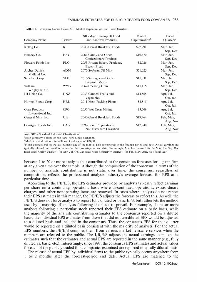
between 1 to 20 or more analysts that contributed to the consensus forecasts for a given firmat any given time over the sample. Although the composition of the consensus in terms of thenumber of analysts contributing is not static over time, the consensus, regardless ofcomposition, reflects the professional analysts industry’s average forecast for EPS at aparticular time.According to the I/B/E/S, the EPS estimates provided by analysts typically reflect earnings

per share on a continuing operations basis where discontinued operations, extraordinarycharges, and other nonoperating items are removed. In cases where analysts do not reporttheir EPS estimates in this manner, the I/B/E/S adjusts the forecast to reflect this. As well, theI/B/E/S does not force analysts to report fully diluted or basic EPS, but rather lets the methodused by a majority of analysts following the stock to prevail. For example, if one or moreanalysts following a particular stock reported their EPS estimate on a basic basis, whilethe majority of the analysts contributing estimates to the consensus reported on a dilutedbasis, the individual EPS estimates from those that did not use diluted EPS would be adjustedto a diluted basis and included in the consensus. Thus, the consensus EPS for that quarterwould be reported on a diluted basis consistent with the majority of analysts. For the actualEPS numbers, the I/B/E/S compiles them from various market newswire services when thenumbers are released to the public. The I/B/E/S adjusts the actual earnings to match theestimates such that the estimates and actual EPS are reported in the same manner (e.g., fullydiluted vs. basic, etc.). Interestingly, since 1998, the consensus EPS estimates and actual valuesfor each of the publicly traded food companies examined are reported on a fully diluted basis.The release of actual EPS by individual firms to the public typically occurs anywhere from

1 to 2 months after the forecast-period end date. Actual EPS are matched to the

TABLE 1. Company Name, Ticker, SIC, Market Capitalization, and Fiscal Quarters

Company Name TickeraSIC-Major Group 20 Food

and Kindred Products

Market

CapitalizationbFiscal

Quartersc

Kellog Co. K 2043-Cereal Breakfast Foods $22,291 Mar, Jun,

Sep, Dec

Hershey Co. HSY 2064-Candy and Other

Confectionary Products

$10,470 Mar, Jun,

Sep, Dec

Flowers Foods Inc. FLO 2053-Frozen Bakery Products,

Except Bread

$2,026 Mar, Jun,

Sep, Dec

Archer Daniels

Midland Co.

ADM 2075-Soybean Oil Mills $21,025 Mar, Jun,

Sep, Dec

Sara Lee Corp. SLE 2013-Sausages and Other

Prepared Meats

$11,831 Mar, Jun,

Sep, Dec

William

Wrigley Jr. Co.

WWY 2067-Chewing Gum $17,115 Mar, Jun,

Sep, Dec

HJ Heinz Co. HNZ 2033-Canned Fruits and

Vegetables

$14,565 Apr, Jul,

Oct, Jan

Hormel Foods Corp. HRL 2011-Meat Packing Plants $4,815 Apr, Jul,

Oct, Jan

Corn Products

International Inc.

CPO 2056-Wet Corn Milling $3,509 Apr, Jul,

Oct, Jan

General Mills Inc. GIS 2043-Cereal Breakfast Foods $19,464 Feb, May,

Aug, Nov

ConAgra Foods Inc. CAG 2099-Food Preparations,

Not Elsewhere Classified

$12,940 Feb, May,

Aug, Nov

Note. SIC5 Standard Industrial Classification.aEach company is listed on the New York Stock Exchange.bMarket capitalization is in millions of dollars as of 9/20/97.cFiscal quarters end on the last business day of the month. This corresponds to the forecast-period end date. Actual earnings are

typically released one month or more after the forecast-period end date. For example, March5 quarter 1 for the Mar, Jun, Sep, Dec

fiscal year; April5 quarter 1 for Apr, Jul, Oct, Jan fiscal year; February5 quarter 1 for Feb, May, Aug, Nov fiscal year.



corresponding forecast-period end date in the database for convenient analysis. The I/B/E/Salso adjusts estimated and actual EPS for mergers and acquisitions, asset write-offs, andcumulative changes in accounting principles that may occur. As well, when a stock splits, theI/B/E/S adjusts all historical forecasts and realized EPS in the database history. Overall, theI/B/E/S ensures that estimated and actual EPS are comparable and appropriately adjusted toaddress the issues associated with using stock data (e.g., basis vs. diluted earnings, splits,accounting changes, and mergers and acquisitions).Given that the focus is on quarterly consensus estimates and actual EPS, the data tend to

exhibit seasonality. For many of the firms, the consensus estimates and actual EPS trendupward over the sample period, consistent with overall growth in earnings for most firmsover the sample period. To account for this seasonality and to ensure stationarity of the data,we focus on quarterly seasonal differences in the data. Specifically, we define the quarterlyforecast series as FEt 5Ft�At�4 where Ft is the consensus forecast for quarter t and At�4 isthe realized EPS for the same quarter of the previous year. We also define the quarterly actualseries as AEt 5At�At�4, which is the difference between the realized EPS in quarter t and therealized EPS in the same quarter of the previous year.3 In both cases, EPS and subsequentlyFEt and AEt are expressed as cents per share.4

Table 2 provides summary statistics (mean and standard deviation) for the quarterlydifference series (FEt and AEt) from 1985.3 to 2007.3. For example, for ADM, the meanseasonal difference FEt is $0.0333 and the mean actual seasonal difference, AEt, is $0.0255.Therefore, consensus analysts’ forecasts over the sample period have estimated on averageabout a 3 cent increase in EPS from the same quarter of the previous year, while realized EPShave averaged about 2.5 cents from the same quarter of the previous year. The consensusestimates and actual EPS have been volatile as well with standard deviations for FEt and AEtfor ADM at $0.0572 and $0.0802, respectively.

4. METHOD AND RESULTS

In this research, we examine several facets of forecast performance of the consensus analysts’forecasts including point accuracy, the forecasts’ optimal properties, as well as their

TABLE 2. Summary Statistics: Forecasted and Actual EPS (cents/share), 1985.3 to 2007.3

Ticker Mean FEt SD FEt Mean AEt SD AEt

K 0.0156 0.0563 0.0256 0.0706

HSY 0.0218 0.0273 0.0214 0.0359

FLO 0.0109 0.0195 0.0098 0.0272

ADM 0.0333 0.0572 0.0255 0.0802

SLE 0.0001 0.0553 0.0058 0.0527

WWY 0.0218 0.0168 0.0235 0.0232

HNZ 0.0371 0.0635 0.0214 0.0551

HRL 0.0213 0.0349 0.0229 0.0414

CPO 0.0342 0.0817 0.0176 0.0692

GIS 0.0287 0.0916 0.0336 0.1090

CAG 0.0145 0.0437 0.0147 0.0607

Note. FEt is the quarterly difference in the consensus analyst forecast for earnings per share (EPS) reported to Institutional Brokers

Estimate System (I/B/E/S) for quarter t ðFt � At�4Þ. AEt is the realized quarterly difference for EPS for quarter t from I/B/E/S

ðAt � At�4Þ. K5Kellogg Co.; H5Hershey Co.; FLO5Flowers Foods Inc.; ADM5Archer-Daniels-Midland Co.; SLE5 Sara Lee

Corp.; WWT5William Wrigley Jr. Co.; HNZ5HJ Heinz Co.; HRL5Hormel Foods Corp.; CPO5Corn Products International

Inc.; GIS5General Mills; CAG5ConAgra Foods Inc.

3Both the series FEt and AEt were found to be stationary using the Augmented Dickey Fuller (ADF) test.4In evaluating forecast errors, the use of year-over-year differences, or difference in successive quarters, is equal.

It can easily be shown that et 5AEt�FEt 5 (At�At�4)�(Ft�At�4)5At�Ft.



improvement over time. In analyzing the performance of consensus EPS forecasts foragribusiness firms, a simple alternative is developed for comparison. Granger (1996) suggeststhe use of simple univariate time-series models for this purpose. Following this advice, weincorporate an AR(4). An AR(4) specification has been used in other studies examiningforecast performance utilizing quarterly data (Sanders & Manfredo, 2002). Although theAR(4) is an admittedly simple alternative, it describes the data well and generally picks up themajor time-series properties of the data. Although other specifications may be moreappropriate than the AR(4) for some of the companies examined, the intention of this studyis not to conduct a horserace of alternative forecasting methods of realized EPS. Rather, theAR(4) merely serves as a straw man to which the consensus forecasts can be compared. Thedata used to estimate the AR(4) are the actual earnings difference (AEt) for each of the firmsbeginning with 1985.3 going through 1993.2 (30 observations), with the corresponding one-period ahead forecast made for 1993.3. Each quarter, the AR(4) model is reestimated andthe one-period ahead forecast made, which results in a growing sample over time to estimatethe one-period ahead forecasts. Hence, the one-period ahead forecast of actual earningschanges (AEt11) corresponding to 2007.3 is estimated using data from 1985.3 to 2007.2(88 observations).Although the AR(4) is a simple model that can be used as a standard of comparison, the

forecasts generated from the AR(4) are inherently at an informational disadvantage to that ofthe consensus forecasts. This is due to the mechanical nature of time-series models, and in thecase of the data used in this research, the reliance on quarterly data. The time-series forecastsonly use information up to the quarter prior to the nearby quarter being forecasted (e.g., pastEPS up to t�1 is used to forecast EPS at time t). Analysts, on the other hand, can adjust theirforecasts up until the last statistical period, which in the case of the consensus forecasts usedin this study is approximately 2 weeks prior to the forecast-period end date. This is illustratedin Figure 1. The only way that the AR(4) could be lined up perfectly with the consensusforecasts is if companies reported their actual earnings on a weekly or biweekly basis, whichis obviously not the case in reality. If this was indeed the case, a forecast could be generatedexactly 2 weeks prior to the forecast-period end date consistent with the last day aconsensus forecast could be adjusted. Each of the evaluation tests and subsequent results areoutlined below.

4.1. Forecast Accuracy and the Mean Absolute Scaled Error

In many studies examining forecast performance, logarithmic changes (percent changes) areused in defining the forecast and actual series (see Sanders & Manfredo, 2002). However,when dealing with forecasted and actual EPS, there is the real possibility of negativeforecasted and realized EPS, which makes the expression of logarithmic changes impossible.Furthermore, many of the forecasted (FEt) and actual changes (AEt) are exact zeroobservations, or very close to zero, which is a natural tendency of earnings data. Thisphenomenon becomes particularly problematic when evaluating forecasts for different dataseries such as we have in this research. That is, forecasted and actual earnings changes for,

etaddnedoireptsaceroFtsacerofsusnesnoctsaLtsacerofseiresemiTmade for quarter t made for quarter t (last day of fiscal quarter)

(analysts can adjust forecasts up to t-2 weeks prior to quarter t)

quarter tquarter t -1 quarter t - 2 weeks

Figure 1 Timing of Consensus and Time Series Forecasts.



say, for the Archer Daniels Midland Company (ADM) may be considerably different fromHormel Foods (HRL). Thus, the data series for the various companies may have differingscale, making it difficult to make comparisons of forecast accuracy across firms, as well asassessments of other forecast properties.In the accounting literature, these issues have be addressed in many ways through various

data manipulations (see O’Brien, 1998, footnote 6, p. 60). For example, Keane and Runkle(1998) normalize predicted and realized EPS by dividing both by the stock price on the lastday of the previous quarter. Brown, Hagerman, Griffen, and Zmijewski (1987) as well asClement (1999) focus their analysis on absolute forecast errors, which by design eliminate theeconomic impact of both negative forecasted and realized earnings. Crichfield et al. (1978), inone of the early studies evaluating analysts’ forecasts, restrict their sample to include onlypositive earnings and realized values. Indeed, many of the procedures used in the accountingliterature are somewhat ad hoc in nature, and may even tamper with economicallymeaningful data points in lieu of reducing statistical problems.Hyndman and Koehler (2006) acknowledge that the aforementioned problems (zero or

near zero observations; scale; negative values) are common with many economic time series.Therefore, in evaluating and comparing the accuracy of economic forecasts with theseproperties, they propose the use of the mean absolute scaled error (MASE) instead of moretraditional accuracy measures such as mean squared error or mean absolute error, which theyclaim may yield infinite or undefined values in the presence of zero values or differing scales.Therefore, we follow Hyndman and Koehler’s suggestion and use the MASE in comparingthe forecast accuracy of analysts’ forecasts versus that of the time-series alternative.The first step in calculating the MASE is to define the scaled error, qt. The forecast error is

defined as et 5AEt�FEt. The forecast error is then scaled by the mean absolute error (MAE)of a naı̈ve, random walk forecast method where the forecast for quarter t is the previousquarter’s realized value (Ft 5At�1). Therefore:

qt ¼et

1n�1

Pni¼2 Ai � Ai�1j j

ð1Þ

where n is the number of observations (Hyndman & Koehler, 2006). The MASE is thensimply:

MASE ¼1

n

Xn

t¼1

jqtj ð2Þ

The MASE’s among competing forecasts can be compared similar to other traditionalaccuracy measures such as mean squared error. That is, the forecast with the smallest MASEwould be considered most accurate among alternatives. Furthermore, when the MASE is lessthan 1, this suggests that the forecast method, on average, provides smaller errors than thatof the one-step, naı̈ve method (Hyndman & Koehler, 2006).In every case the consensus forecasts have a smaller MASE than that of the time-series

forecasts (Table 3). This is consistent with the extant literature from the accounting field,which suggests that analysts’ forecasts tend to be more accurate than those provided fromcompeting models, in particular time-series models (Barefield & Comiskey, 1975; Brown &Rozeff, 1978; Hopwood, McKeown, & Newbold, 1982). As well, in each case for theconsensus forecasts, the MASE is less than 1 suggesting improvement relative to the naı̈ve no-change forecast. Only the MASE for ADM is reasonably close to 1 (0.9640). Interestingly, thetime-series forecasts perform quite well relative to the random walk naı̈ve model, with onlyADM being greater than 1 (1.125) and HNZ approaching 1 (0.9887). However, it may be thecase that the differences in forecast accuracy between the consensus forecasts and the timeseries alternative, as measured by the MASE, are not statistically significant (Diebold &Mariano, 1995).To test this hypothesis, we incorporate the modified Diebold-Mariano (MDM) statistic for

testing the differences in mean squared errors as suggested by Harvey, Leybourne, and



Newbold (1997).5 The MDM test uses two time series of h-step ahead forecast errors, e1t ande2t, (t5 1 to n) and a specified loss function g(e). For this research, e1t and e2t are replaced withthe respective scaled series q1t and q2t, where q1t corresponds to the scaled forecast errors of theconsensus forecasts and q2t to the scaled forecast errors of the time-series forecasts. The nullhypothesis of the MDM test is E[g(q1t)�g(q2t)]5 0, where the loss function, g(e), is the absolutevalue operator in the case of MASE. Rejection of the null hypothesis suggests that there is astatistically significant difference between the accuracy of the compared forecasts. The nullhypothesis that the sample mean ( �d) of dt 5 g(q1t)�g(q2t)5 0 is tested using the critical valuesfrom a t-distribution. The MDM statistics are presented in Table 3.Although the consensus forecasts have a smaller MASE in each case relative to the time-

series benchmark forecasts, in only four instances are the differences statistically significant.Only the consensus estimates for K, FLO, ADM, and SLE are statistically smaller than thetime-series alternative at the 5% level (4 out of 11 instances). Though certainly notunanimous, these results on average suggest that analysts provide more accurate forecaststhan simple time-series alternatives, namely the AR(4), which is consistent with findings inthe accounting and finance literature. However, the improvement is not statisticallysignificant for most of the stocks examined in the sample. Although understanding thepoint accuracy of a forecast is important, it is only one measure of overall forecastperformance.

4.2. Test for Forecast Bias

An optimal forecast is one that is both unbiased and efficient (Diebold & Lopez, 1998). Anoptimal forecast utilizes all information available to the forecaster. It is also the mostaccurate forecast in a mean squared error framework. Typically, forecast optimality is testedusing the following ordinary least squares (OLS) regression framework:

ACTt ¼ a1bFCSTt1et; ð3Þ

TABLE 3. Mean Absolute Scaled Error (MASE), 1993.3 to 2007.3

Ticker Consensus Time Series MDM testa MAE Naiveb

K 0.2269 0.5551 2.0793� 0.0897

HSY 0.0966 0.1835 0.1470 0.1319

FLO 0.5953 0.7700 �3.6674� 0.0263

ADM 0.9640 1.1252 �2.6515� 0.0533

SLE 0.1567 0.4704 2.4155� 0.0790

WWY 0.2953 0.4284 �0.9493 0.0419

HNZ 0.6039 0.9887 �0.3187 0.0406

HRL 0.2476 0.3214 0.0428 0.1016

CPO 0.2287 0.3145 �1.0861 0.1701

GIS 0.1686 0.4377 0.6358 0.1619

CAG 0.2230 0.4334 0.7671 0.1174

Note. K5Kellogg Co.; H5Hershey Co.; FLO5Flowers Foods Inc.; ADM5Archer-Daniels-Midland Co.; SLE5Sara Lee Corp.;

WWT5William Wrigley Jr. Co.; HNZ5HJ Heinz Co.; HRL5Hormel Foods Corp.; CPO5Corn Products International Inc.;

GIS5General Mills; CAG5ConAgra Foods Inc.�Significant at the 5% level.aThe t-statistics are from the Modified Diebold-Mariano Test (MDM) for equality in prediction errors (see Harvey, Leybourne, &

Newbold, 1997).bMAE Naı̈ve is the mean absolute error from a naı̈ve, random walk forecasting model where the forecast, Ft, is the previous quarter’s

actual EPS, At�4, and hence the error defined as et ¼ At � At�1. The MAE Naı̈ve serves as the scaler, x, in the development of the

scaled error terms, qt.

5The MDM statistic can be adapted for use with any evaluation metric including the proposed MASE statistic. In

the case of MASE, et is replaced by the scaled errors qt.



where ACTt is the realized value and FCSTt is the forecast. The joint null hypothesis forforecast optimality is that a5 0 and b5 1. Failure to reject the joint null implies that theforecast is indeed optimal in that it is both unbiased, a5 0, and efficient b5 1. This commontest, however, is subject to interpretative problems (Granger & Newbold, 1986; Holden &Peel, 1990). Namely, the joint null is only a necessary condition for efficiency (Granger &Newbold, 1986) and a necessary, but not sufficient, condition for unbiasedness. A rejection ofthe null hypothesis, therefore, does not provide clear insight into the optimal properties of theforecast. Therefore, to avoid these interpretive problems, we use the methodologydemonstrated by Pons (2000) which incorporates the suggestion by Granger and Newbold(1986, p. 286) that forecast optimality tests should be conducted using forecast errors(Holden & Peel, 1990). For this research, we modify this suggestion slightly and continue ourevaluation using scaled forecast errors, qt.The specific test for bias used here is an OLS regression of the scaled forecast error, qt, on

an intercept term (g) such that:

qt ¼ g1ut; ð4Þ

where ut is a random disturbance term (Pons, 2000). The null hypothesis of an unbiasedforecast, one that does not consistently under- or overestimate the actual value, is g5 0. Thenull hypothesis is tested using a two-tailed t test.6

Table 4 shows the results of the forecast bias test outlined in Equation 4. Of the 11 firmsexamined, only the consensus forecasts for K and SLE are found to exhibit a statisticallysignificant bias at the 5% level. In other words, the majority of the consensus forecasts areunbiased. In both cases where a statistically significant bias is found, the consensus forecastssystematically underestimate the actual EPS (g40). Overall, these findings suggest thatanalysts’ forecasts perform reasonably well as a group in terms of providing unbiasedpredictions of future EPS—an important aspect of forecast optimality. Likewise, as is

TABLE 4. Test for Forecast Bias (qt 5 g1ut), 1993.3 to 2007.3

Consensus Time Series

g t-Stat p-Value g t-Stat p-Value

K 0.1512 3.7600 0.0004 �0.0069 �0.0703 0.9442

HSY 0.0045 0.2478 0.8051 0.0002 0.0067 0.9947

FLO �0.0380 �0.3528a 0.7255 0.3079 1.9556a 0.0553

ADM �0.1625 �0.7738a 0.4422 0.2478 1.2804 0.2055

SLE 0.0944 2.7353a 0.0083 �0.1438 �1.4548 0.1511

WWY 0.0008 0.0153 0.9879 0.0537 0.6537a 0.5159

HNZ �0.0672 �0.5002 0.6188 �0.0037 �0.0239a 0.9810

HRL 0.0342 0.8187a 0.4163 0.0320 0.5497 0.5846

CPO �0.0702 �0.8407a 0.4040 0.0089 0.1521 0.8797

GIS 0.0262 0.6125 0.5426 �0.0188 �0.2255 0.8224

CAG 0.0166 0.2796a 0.7808 �0.0386 �0.5105a 0.6116



GIS5General Mills; CAG5ConAgra Foods Inc.aStandard error estimated with Newey-West covariance estimator.

6The data setup used in this study yields non-overlapping forecasts and actual values of quarterly EPS. Therefore,

the OLS standard errors from this and all subsequent regression models are consistent (Brown & Maital, 1981;

Clements & Hendry, 1998, p. 57). In Equation 4, and in all subsequent regression models, heteroskedasticity is tested

using White’s test. Serial correlation is tested using the Ljung-Box test. If heteroskedasticity is found, White’s

heteroskedastic consistent covariance estimator is used. If serial correlation is present, the Newey-West covariance

estimator is used (Hamilton, 1994, p. 218).



expected, there is a failure to reject the null hypothesis of g5 0 for the time-series forecasts ofEPS for each firm (5% level), illustrating that each of the time-series forecasts are unbiased.

4.3. Tests for Forecast Efficiency—Beta and Rho Efficiency

Forecast efficiency is another critical component of forecast optimality. A forecast is said tobe weakly efficient if forecast errors, et, are orthogonal to the forecasts themselves andorthogonal to past forecast errors (Nordhaus, 1987). Given this, the following regressionframework is used to test for weak efficiency in the scaled forecast errors qt of the consensusand time-series forecasts of EPS (Pons, 2000):

qt ¼ a1bFEt1ut ð5Þ

and

qt ¼ a1rqt�11ut: ð6Þ

Equation 5 is referred to as the beta efficiency test (Table 5). Here, the null hypothesis offorecast efficiency is b5 0. If the null hypothesis is rejected, this suggests that the forecast isnot a minimum variance forecast. That is, the forecast, FEt, is not efficiently or optimallyincorporating all information available regarding future EPS available at period t. If b40,the forecasts are systematically too conservative, and if bo0, the forecasts are systematicallytoo optimistic or too extreme.Equation 6 is the rho efficiency test (Table 6), which tests if forecast errors are

systematically related to past forecast errors. If the null hypothesis of r5 0 is rejected (two-tailed t test), then forecast errors in time t are related to past errors. In the case that r40, thissuggests that past forecast errors are repeated (e.g., positive autocorrelation). For example,an overestimate of AEt would likely be followed by another overestimate and visa-versa. Ifro0, then overestimates would be followed by underestimates and visa-versa.Table 5 presents the results of the beta efficiency test from Equation 5. The consensus

forecasts for 5 of the 11 firms are rejected for beta efficiency (HSY, SLE, WWY, HNZ, andCPO) at the 5% level, and one (K) at the 10% level. This suggests that analysts are notefficiently using the information available regarding future EPS for these firms at the time theconsensus forecast is computed. Interestingly, the consensus forecasts for both K and SLE werealso found to be systematically biased as discussed earlier. Four of the seven firms (SLE, HNZ,

TABLE 5. Test for Beta Efficiency (qt 5 a1bFEt1ut), 1993.3 to 2007.3


Ticker b t-Stat p-Value b t-Stat p-Value

K 1.2019 1.9276 0.0589 �2.1180 �0.9074 0.3680

HSY 1.4319 3.3970b 0.0012 �0.2825 �0.2288 0.8198

FLO �5.3708 �0.9091 0.3671 �5.4089 �0.6744 0.5028

ADM 0.4697 0.1622a 0.8717 �4.2113 �1.5942 0.1164

SLE �1.2189 �2.4390a 0.0179 �3.5953 �1.4869a 0.1426

WWY 6.8260 2.1124 0.0390 �13.2598 �1.6871b 0.0971

HNZ �7.3997 �2.0197a 0.0481 �9.1739 �1.8402b 0.0710

HRL �1.9094 �1.4855a 0.1429 �3.5976 �1.5021 0.1386

CPO �2.2650 �2.3430a 0.0226 �2.5413 �2.2058 0.0314

GIS �0.0076 �0.0168 0.9867 �1.9502 �0.9099b 0.3667

CAG 1.0362 1.1660a 0.2485 �7.8022 �3.6875 0.0005



GIS5General Mills; CAG5ConAgra Foods Inc.aStandard error estimated with Newey-West covariance estimator.bStandard error estimated with White’s covariance estimator.



HRL, and CPO) had bo0, and three firms realized b40 (K, HSY, and WWY). For example,b5�7.3997 for HNZ suggests that the forecast errors are negatively related to the consensusforecast such that a large positive forecast generates a large negative error, and that a largenegative forecast generates a large positive error. Interestingly, the time-series forecasts forCPO, HNZ, WWY, and CAG were also found to be beta inefficient. Although the AR(4) is arelatively simple model that is applied across the various stocks to serve as a simple comparisonto the consensus forecasts, this result suggests that the AR(4) may not be the most appropriatetime-series model in terms of forecasting ability. These results may also be illustrating the factthat time-series models in general are inherently penalized in forecasting quarterly EPS giventhat time-series models can only use data up to the prior quarter, whereas analysts canassimilate new information into their forecasts up to the last statistical period prior to theforecast-period end date.Results from the rho efficiency tests are presented in Table 6. The null hypothesis of r5 0 is

rejected for the consensus forecasts of ADM and CPO at the 5% level ( p-value5 0.0139 and0.0002, respectively). In each case, the estimated r40 suggests that past forecast errors arerepeated. That is, there is some positive autocorrelation in the error terms. Although it isdifficult to determine the exact reasons underlying these findings, it may be that analysts arenot adequately capturing structural changes or other phenomenon related to these firms.ADM and CPO are also firms that are directly involved in the grain trade. It may be thatanalysts are not adequately incorporating information regarding the volatility of commodityprices that may ultimately impact EPS of these firms. Considering these results relative to thetime-series benchmark, for each stock there is a failure to reject the null hypothesis at the 5%level. Given that the time series models rely on serial correlation in generating forecasts, thesefindings are not surprising. Interestingly, however, the null hypothesis of the time seriesforecast for ADM and WWY are rejected at the 10% level ( p-value5 0.0729 and 0.0912,respectively). Indeed, this at least somewhat suggests that time-series behavior in the errorterms is not adequately being captured by the AR(4) model, which was applied uniformly toall series for comparative purposes. Although it may be a matter of misspecification of thetime-series model (e.g., a more appropriate time-series specification exists for ADM andWWY), it may also be systematic structural changes or other phenomenon, such as volatilityin commodity prices, which is causing forecast errors to be repeated regardless of how theforecast is formed. This finding may also be due to nonsystematic factors strictly unique toADM and WWY. Overall, the results from the rho efficiency test suggests that at least for the

TABLE 6. Test for Rho Efficiency (qt 5 a1ret�11ut), 1993.3 to 2007.3


Ticker r t-Stat p-Value r t-Stat p-Value

K 0.1274 0.9663 0.3381 0.1512 1.1482 0.2558

HSY 0.0582 0.4179 0.6776 0.0582 0.4179 0.6776

FLO �0.1182 �0.8857 0.3796 �0.1182 �0.8857 0.3796

ADM 0.3294 2.5409 0.0139 0.2500 1.8301 0.0726

SLE 0.0442 0.5424a 0.5897 0.0881 0.6616 0.5109

WWY 0.1517 1.1493 0.2553 0.2273 1.7184 0.0912

HNZ 0.3655 1.7688a 0.0824 �0.1687 �1.2688 0.2098

HRL �0.0884 �0.9840a 0.3293 0.0320 0.2361 0.8142

CPO 0.7172 3.9177b 0.0002 �0.0699 �0.5200 0.6051

GIS 0.2253 1.7308 0.0890 0.1777 1.3626 0.1785

CAG 0.0967 0.4906a 0.6256 �0.2713 �1.1303b 0.2632






case of ADM and CPO, the consensus forecasts may not be capturing or reflecting somerelevant time-series behavior in the actual quarterly changes in EPS.

4.4. Test for Forecast Encompassing

A preferred forecast is said to encompass a competing or alternative forecast if there is nolinear combination of forecasts (e.g., a composite forecast) that would yield a smaller meansquared error relative to the preferred (Mills & Pepper, 1999). If this is the case, then thecompeting forecast contains no useful information that is not already found in the preferredforecast (Harvey, Leybourne, & Newbold, 1998).7 Forecast encompassing is tested in thefollowing regression framework (Harvey et al., 1998):

q1t ¼ a1lðq1t � q2tÞ1ut ð7Þ

where q1t are the scaled errors from the preferred forecast, q2t are the scaled errors from thecompeting forecast, q1t�q2t is the difference in the two forecast error series, and ut is arandom disturbance term. The null hypothesis is l5 0. A rejection of the null hypothesissuggests that the preferred and competing forecasts can be combined to form a compositeforecast that would result in a smaller squared error than the preferred forecast alone. In thiscase, the weight placed on the competing forecast would be the estimated l and the weightplaced on the preferred forecast would be 1�l. A failure to reject the null hypothesis suggeststhat the preferred forecast should be used by itself given it encompasses the information fromthe competing forecasts.The OLS estimates corresponding to Equation 7 are presented in Table 7. Table 7 is broken

into two sections for comparative purposes. In the first set of results, the consensus forecast isdesignated as the preferred forecast. According to the encompassing test, the null hypothesisof forecast encompassing is rejected at the 5% level for K ( p-value5 0.0004), HNZ( p-value5 0.0119), HRL ( p-value5 0.0400), and CPO (p-value5 0.0006). This suggests thatthe consensus EPS forecasts for each of these companies could be combined with the time-series forecasts to provide a forecast that has a smaller mean squared error relative to thepreferred. Interestingly and not surprisingly the consensus forecasts for CPO, which wasfound to be rho inefficient earlier, could be improved by combining with time-series forecasts.However, this was not the case for the consensus forecasts for ADM, which were alsofound to be rho inefficient at the 5% level. However, l is significant at the 10% level(p-value5 0.0602) for ADM, providing at least some evidence that analysts are notadequately incorporating the time-series properties of actual EPS when making theirforecasts. In the case of CPO, the optimal weight to place on the time-series forecast would be0.5996 (1�0.4004), and the weight to place on the consensus forecast would be l5 0.4004.The composite weights for the other consensus forecasts where a significant l was foundinclude 0.2367 and 0.7633 for HRL, 0.3129 and 0.6871 for HNZ, and �0.1923 and 1.1923 forK. In the case for K, a negative weight is placed on the consensus forecast whereas a positiveweight is placed on the time-series alternative. Although the signs on these weights aresomewhat unexpected, they are a result of the covariance relationship between the consensusforecast and the time series alternative (Harvey et al., 1998).When the preferred forecast is designated as a time-series forecast, the null hypothesis of

l5 0 is rejected for each of the firms in the sample. This result confirms that the time-seriesforecasts alone will not provide the smallest mean squared error. For example, in the case ofthe consensus forecasts for GIS, the null hypothesis of forecast encompassing (l5 0) cannotbe rejected. This suggests that the consensus forecasts used on their own will provide thesmallest mean squared error and that a composite forecast with the time-series alternativewill provide no improvement relative to the consensus forecast. When the preferred forecast

7Note that the use of the word ‘‘preferred forecast’’ does not insinuate that the particular forecast is indeed

preferred to others. Rather, it is nomenclature typically used in the forecasting literature when comparing two

forecasts in an encompassing framework.



is designated as the time series alternative, l5 0 is rejected at the 5% level with l5 1.0137.This suggests that in a composite forecast with the consensus forecast, that basically allweight should be placed on the consensus forecast and none on the time-series alternative.The fact that the consensus forecasts for more than half the firms in the sample are found

not to encompass the simple time-series alternative at either the 5% or 10% level suggeststhat professional analysts may not be doing a good job of incorporating the time seriesproperties of past realized EPS into their forecasts. That is, for the instances where the null ofl5 0 is rejected, the consensus is systematically ignoring or failing to properly incorporatethe time-series properties of historical EPS. This result is especially compelling given that thetime series alternative is inherently penalized relative to the consensus forecasts from aninformational perspective. This result is likely not to change even if the time-series forecastswere perfectly aligned with the consensus forecasts. Given that analysts contributing to theconsensus can actually update their forecasts up to 2 weeks prior to the forecast-period enddate, this result is especially interesting. Although it seems odd that analysts wouldsystematically ignore this information, it is easy to ponder situations where individualanalysts would fail to incorporate the time-series behavior of past EPS. For example, theanalyst may base their estimates strictly based on their judgment, their own model, or otherfundamental factors such as inherent knowledge of the firm, its management, product mix,etc., which does not formally or informally incorporate information in historical EPS.

4.5. Tests for Forecast Improvement

The final test used examines if the consensus forecasts have improved over time. A test forforecast improvement is presented here following the methodology of Bailey and Brorsen(1998). Again, focusing on scaled forecast errors, the test for forecast improvement is defined as:

jqtj ¼ d11d2Trendt1ut ð8Þ

where |qt| is the absolute value of the scaled forecast error and Trendt is a time trend. The nullhypothesis is that d2 5 0, which is tested with a two-tailed t test. A failure to reject the nullhypothesis implies that there is not a systematic improvement or deterioration in the absolutescaled forecast errors over time. A rejection of the null hypothesis, on the other hand,suggests that forecast errors have become systematically smaller (d2o0) or systematicallylarger (d240) over time.

TABLE 7. Test for Forecast Encompassing q1t ¼ a1lðq1t � q2tÞ1ut, 1993.3 to 2007.3

Preferred Forecast-Consensus Preferred Forecast-Time Series

Ticker l t-Stat p-Value l t-Stat p-Value

K �0.1923 �3.7751a 0.0004 1.1923 23.4102a 0.0000

HSY �0.1002 �1.0420 0.3018 1.1002 11.4420 0.0000

FLO 0.3327 1.9160 0.0604 0.6673 3.8427 0.0003

ADM 0.2551 1.9173 0.0602 0.7449 5.5989 0.0000

SLE 0.0640 1.3834a 0.1719 0.9360 20.2364a 0.0000

WWY �0.1853 �1.5029 0.1384 1.1853 9.6126 0.0000

HNZ 0.3129 2.5992b 0.0119 0.6871 5.7073 0.0000

HRL 0.2367 2.1013 0.0400 0.7633 6.7762 0.0000

CPO 0.4004 3.6407b 0.0006 0.5996 5.4522 0.0000

GIS �0.0137 �0.1714 0.8645 1.0137 12.6799 0.0000

CAG �0.0654 �0.9538a 0.3442 1.0654 15.5479 0.0000

Note. K5Kellogg Co.; H5Hershey Co.; FLO5Flowers Foods Inc.; ADM5Archer-Daniels-Midland Co.; SLE5 Sara Lee Corp.;





Results of Equation 8 are reported in Table 8. For the consensus forecasts, d2 is 40 for allfirms but HNZ and CPO. In five cases, nearly half of the sample firms, the null hypothesis ofd2 5 0 is rejected at the 5% level (K, FLO, SLE, WWY, and CAG). These results suggest thaton average, consensus analysts’ forecasts have not improved over time, but have actuallybecome systematically larger. Interestingly, similar results are found for the time seriesforecasts. In 7 out of 11 cases the null hypothesis of d2 5 0 is rejected at the 5% level. In fact,the null hypothesis for both the consensus forecasts and time-series forecasts are rejected forFLO, SLE, WWY, and CAG. The fact that there is systematic deterioration in both theconsensus forecasts and time-series forecasts implies that it may be getting increasinglydifficult to forecast earnings for these firms. This particularly may be the case for the year2000 and beyond.Indeed, since year 2000, firm-level profitability has become more variable for many

agribusiness firms given volatility in commodity markets, increased financial reportingregulation, and associated regulatory costs (e.g., Sarbanes-Oxley), consolidation in the foodand agribusiness sector, globalization, among other systematic factors (e.g., the 9/11 terroristattack) and nonsystematic factors alike (e.g., mergers and acquisitions). As well, in theaftermath of Enron and other corporate scandals, many analysts that worked for investmentbanking firms quit, were fired, or were forced to separate their analysis work from thebrokerage functions of the firms that they worked for. Therefore, there was likely a largeturnover of analysts post-2000 that may have contributed to increased forecast errors overtime. Figure 2 shows the plots of absolute forecast errors (nonscaled) for consensus forecastsand time-series forecasts for SLE and CAG (two companies for which there was statisticallysignificant deterioration in both the consensus and time-series forecasts). Indeed, a pattern ofincreasing and more volatile forecast errors over time is evident, in particular post-2000.

5. SUMMARY, CONCLUSIONS, AND IMPLICATIONS

This research provides a comprehensive examination of the forecasting performance ofprofessional analysts’ forecasts of EPS for a sample of publicly traded food companies. Inparticular, consensus estimates of EPS provided through the I/B/E/S, a division ofThompson Financial, were examined. As well, simple time-series alternative forecastsgenerated by an AR(4) model served as a point of comparison to the consensus forecasts.The food companies examined represent some of the largest agribusiness firms listed on the

TABLE 8. Test for Improvement Over Time (jqtj5 d11d2Trendt1ut), 1993.3 to 2007.3


Ticker d t-Stat p-Value d t-Stat p-Value

K 0.0053 2.8515 0.0060 �0.0003 �0.0694 0.9449

HSY 0.0003 0.4403 0.6613 0.0032 2.5928 0.0121

FLO 0.0143 3.6443a 0.0006 0.0181 3.4440a 0.0011

ADM 0.0020 0.3380 0.7366 0.0276 3.6857b 0.0005

SLE 0.0070 4.2464 0.0001 0.0207 6.8464a 0.0000

WWY 0.0064 3.2837 0.0018 1.0149 3.7894b 0.0004

HNZ �0.0039 �0.4377b 0.6633 0.0179 2.5080 0.0150

HRL 0.0023 1.2328 0.2227 �0.0014 �0.5763 0.5667

CPO �0.0072 �1.6156a 0.1117 �0.0019 �0.6385a 0.5257

GIS 0.0017 0.7666 0.4465 0.0039 1.1548a 0.2530

CAG 0.0101 5.4108a 0.0000 0.0104 2.9439a 0.0047






New York Stock Exchange, each reflecting a market capitalization of more than $2 billion.Analysts’ estimates of EPS provide a rare source of forward-looking informationregarding firm-level financial performance. Indeed, the decisions made by large publiclytraded agribusiness firms likely impact downstream players and even rural communities(Vickner, 2002).

SLE

0

0.5

1

1.5

2

2.5

3

Mar

-93

Sep

-93

Mar

-94

Sep

-94

Mar

-95

Sep

-95

Mar

-96

Sep

-96

Mar

-97

Sep

-97

Mar

-98

Sep

-98

Mar

-99

Sep

-99

Mar

-00

Sep

-00

Mar

-01

Sep

-01

Mar

-02

Sep

-02

Mar

-03

Sep

-03

Mar

-04

Sep

-04

Mar

-05

Sep

-05

Mar

-06

Sep

-06

Mar

-07

Sep

-07

cen

ts/s

har

e

CAG

0

0.5

1

1.5

2

2.5

3

Mar

-93

Sep

-93

Mar

-94

Sep

-94

Mar

-95

Sep

-95

Mar

-96

Sep

-96

Mar

-97

Sep

-97

Mar

-98

Sep

-98

Mar

-99

Sep

-99

Mar

-00

Sep

-00

Mar

-01

Sep

-01

Mar

-02

Sep

-02

Mar

-03

Sep

-03

Mar

-04

Sep

-04

Mar

-05

Sep

-05

Mar

-06

Sep

-06

Mar

-07

Sep

-07

cen

ts/s

har

e

consensustime series

consensustime series

Figure 2 Absolute Value of Scaled Forecast Errors (jqtj), 1993.3–2007.3.



The results from the forecast accuracy tests (MDM test comparing mean absolute scalederrors), test for forecast bias, test for beta efficiency, test for rho efficiency, forecastencompassing tests, and tests for forecast improvement are summarized in Table 9 for each ofthe food companies in the sample. Overall, although the results are mixed, there isconsiderable evidence suggesting that the analyst community as a whole, as reflected througha consensus EPS forecast, may not be doing well in predicting EPS for these firms. Forexample, for Kellogg (K), consensus forecasts provide more accurate point forecasts than thetime-series alternative, which is statistically significant, but they are also biased, betainefficient, and forecast errors have systematically increased over time. As well, consensusEPS forecasts for K do not encompass time series information provided by the time-seriesalternative. The consensus forecasts for Flower Foods (FLO), Archer Daniel’s Midland(ADM), and Sara Lee (SLE) all have a MASE that is smaller than that produced by the time-series alternative (statistically significant at the 5% level), but all fail in some other measure offorecast performance. For example, the consensus forecasts for SLE are found to besystematically biased, inefficient, and forecast errors have increased over time. The consensusforecasts for FLO and ADM both fail to encompass the information contained in a simpletime-series alternative, and in the case of ADM, forecast errors tend to be repeated althoughthey have increased over time for FLO. For HJ Heinz (HNZ), and Corn ProductsInternational (CPO), there is evidence that the consensus forecasts of EPS are not statisticallymore accurate than the time-series alternative, are both beta and rho inefficient, and do notencompass the information in the time-series forecasts. In terms of the optimal properties offorecasts (bias, efficiency, and forecast encompassing), the consensus forecasts for ConAgra(CAG) performed the best. However, forecast errors have systematically increased over time,and point accuracy is not statistically significant relative to a simple time-series alternative.Although these results suggest that as a group, analysts that follow food companies

produce EPS forecasts that are less than optimal, it may be the case that EPS is just becomingmore difficult to forecast in the food industry. This may be the result of a number of issuesincluding volatility of commodity prices, globalization, consolidation in the agribusinessindustry, regulatory changes (e.g., Sarbanes-Oxley), which have modified the investmentbanking and analyst environment, as well as generalized EPS volatility due to systematicinfluences in the economy postyear 2000 (e.g., 9/11, Enron, Iraq and Afghanistan wars,

TABLE 9. Summary of Forecast Performance Tests for Consensus Forecasts

Ticker MDMaBiasb

a5 0

Beta

Efficiency

b5 0

Rho

Efficiency

r5 0

Forecast

Encompassing

l5 0

Forecast

Improvement

d2 5 0

K 5% 10% 5% 5%

HSY X 5%

FLO 10% 5%

ADM 5% 10%

SLE 5% 5% 5%

WWY X 5% 5%

HNZ X 5% 10% 5%

HRL X 10% 5%

CPO X 5% 5% 5%

GIS X 10%

CAG X 5%



GIS5General Mills; CAG5ConAgra Foods Inc.aX signifies that the modified Diebold-Mariano test for equality of mean absolute scaled errors (MASEs) is not significant at the 5%

level. Therefore, although the consensus forecast has a smaller MASE than the time series alternative, it is not statistically significant.b5% reflects that the null hypothesis of the respective test was rejected at the 5% level. 10% represents that the null hypothesis of the

respective test was rejected at the 10% level.



interest rate environment, housing bubble, and general economic conditions). Still, analysts’forecasts of EPS provide one of the few, if only, forward-looking estimates of financialperformance for publicly traded companies. Thus, decision makers in the food andagribusiness sector should be cognizant of the forecast performance of EPS estimates forthese companies given their influence across the agro-food supply chain.This study provides practical insight into the performance of these forecasts such that

managers can more efficiently use analysts’ estimates in their overall decision making. Froman academic perspective, the results presented here for food companies help to corroborate thefindings generalized in the accounting and finance literature—that is analysts’ forecasts tend tobe more accurate than alternative forecasts, but are not necessarily rational. Furthermore, thisresearch introduces the mean absolute scaled error approach for comparing forecast accuracy,which is useful when forecast error observations are often zero or close to zero, or of differingscale, as is often the case when dealing with earnings data. As well, this study utilizes forecastevaluation techniques commonly used in the agricultural economics literature to examine theperformance of analysts’ EPS forecasts for publicly traded agro-food companies. Indeed, untilnow, evaluation of EPS forecasts and related issues has remained the privy of accounting andfinance scholars. Given the impact that large, publicly traded agribusiness firms have on theentire agro-food chain, it is critical that agribusiness scholars take ownership of this andsimilar lines of research such that we can better understand the behavior and performance ofthese firms and their potential impacts.

REFERENCES

Affleck-Graves, J., Davis, L.R., & Mendenhall, R.R. (1990). Analyst superiority and bias. ContemporaryAccounting Research, 6, 501–517.

Bailey, D.V., & Brorsen, B.W. (1998). Trends in the accuracy of USDA production forecasts for beef and pork.Journal of Agricultural and Resource Economics, 23, 515–525.

Barefield, R.M., & Comiskey, E.E. (1975). The accuracy of analysts’ forecasts of earnings per share. Journal ofBusiness Research, 3, 241–252.

Brown, B.W., & Maital, S. (1981). What do economists know? An empirical study of expert’s expectations.Econometrica, 49, 491–504.

Brown, L.D., Hagerman, R.L., Griffen, P.A., & Zmijewski, M.E. (1987). Security analyst superiority relative tounivariate time series models in forecasting quarterly earnings. Journal of Accounting and Economics, 9, 61–87.

Brown, L.D., & Rozeff, M.S. (1978). The superiority of analyst forecasts as measures of expectations: Evidence fromearning. The Journal of Finance, 33, 1–16.

Burgstahler, D., & Eames, M. (2006). Management of earnings and analysts’ forecasts to achieve zero and smallpositive earnings surprises. Journal of Business Finance and Accounting, 33, 633–652.

Capstaff, J., Paudyal, K., & Rees, W. (1995). The accuracy and rationality of earnings forecasts by UK analysts.Journal of Business Finance and Accounting, 22, 67–85.

Carter, C.A., & Galopin, C.A. (1993). Informational content of government hogs and pigs reports. American Journalof Agricultural Economics, 75, 711–718.

Clement, M.B. (1999). Analyst forecast accuracy: Do ability, resources, and portfolio complexity matter. Journal ofAccounting and Economics, 27, 285–303.

Clements, M.P., & Hendry, D.F. (1998). Forecasting economic time series. Cambridge: Cambridge University Press.Crichfield, T., Dyckman, T., & Lakonishok, J. (1978). An evaluation of security analysts’ forecasts. The Accounting

Review, 53, 651–668.Das, S., Levine, C.B., & Sivaramakrishnan, K. (1998). Earnings predictability and bias in analysts’ earnings

forecasts. The Accounting Review, 73, 277–294.Diebold, F.X., & Lopez, J.A. (1998). Forecast evaluation and combination. In G.S. Maddala & C.R. Rao (Eds.),

Handbook of statistics 14: Statistical methods in finance. Amsterdam: North-Holland.Diebold, F.X., & Mariano, R.S. (1995). Comparing predictive accuracy. Journal of Business and Economic Statistics,

13, 253–263.Francis, J., & Philbrick, D. (1993). Analysts’ decisions as products of multi-task environment. Journal of Accounting

Research, 31, 216–230.Garcia, P., Irwin, S.H., Leuthold, R.M., & Yang, L. (1997). The value of public information in commodity futures

markets. Journal of Economic Behavior and Organization, 32, 559–570.Granger, C.W.J. (1996). Can we improve the perceived quality of economic forecasts? Journal of Applied

Econometrics, 11, 455–473.Granger, C.W.J., & Newbold, P. (1986). Forecasting economic time series (2nd ed.). New York: Academic Press.



Hamilton, J.D. (1994). Time series analysis. Princeton, NJ: Princeton University Press.Harvey, D.I., Leybourne, S.J., & Newbold, P. (1997). Testing the equality of prediction mean squared errors.

International Journal of Forecasting, 13, 281–291.Harvey, D.I., Leybourne, S.J., & Newbold, P. (1998). Tests for forecast encompassing. Journal of Business and

Economic Statistics, 16, 254–259.Ho, L.C.J. (1996). Bias and accuracy of analysts’ forecasts: Evidence from Australia. International Journal of

Management, 13, 306–313.Holden, K., & Peel, D.A. (1990). On testing for unbiasedness and efficiency of forecast. The Manchester School, 15,

120–127.Hong, H., & Kubik, J.D. (2003). Analyzing the analysts: Career concerns and biased earnings forecasts. Journal of

Finance, 58, 313–351.Hopwood, W.S., McKeown, J.C., & Newbold, P. (1982). The additional information content of quarterly earnings

reports: Intertemporal disaggregation. Journal of Accounting Research, 20, 343–349.Hunton, J.E., & McEwen, R.A. (1997). An assessment of the relation between analysts’ earnings forecast accuracy,

motivational incentives and cognitive information search strategy. The Accounting Review, 72, 497–515.Hyndman, R.J., & Koehler, A.B. (2006). Another look at measures of forecast accuracy. International Journal of

Forecasting, 22, 679–688.Kastens, T.L., Schroeder, T.C., & Plain, R. (1998). Evaluation of extension and USDA price and production

forecasts. Journal of Agricultural and Resource Economics, 23, 244–261.Keane, M.P., & Runkle, D.E. (1998). Are financial analysts’ forecasts of corporate profits rational. Journal of

Political Economy, 106, 768–805.Lim, T. (2001). Rationality and analysts’ forecast bias. Journal of Finance, 46, 285–369.McNichols, M.F., & O’Brien, P.C. (1997). Self-selection and analyst coverage. Journal of Accounting Research, 35,

167–199.Mills, T.C., & Pepper, G.T. (1999). Assessing the forecasters: An analysis of the forecasting records of the Treasury,

the London Business School, and the National Institute. International Journal of Forecasting, 15, 247–257.Nordhaus, W.D. (1987). Forecasting efficiency: Concepts and applications. The Review of Economics and Statistics,

69, 667–674.O’Brien, P.C. (1998). Analysts’ forecasts as earnings expectations. Journal of Accounting and Economics, 10, 53–58.Pons, J. (2000). The accuracy of IMF and OECD forecasts for G7 countries. Journal of Forecasting, 19, 53–63.Ramnath, S., Rock, S., & Shane, P. (2008). The financial analyst forecasting literature: A taxonomy with suggestions

for further research. International Journal of Forecasting, 24, 34–75.Sanders, D.R., & Manfredo, M.R. (2002). USDA production forecasts for pork, beef, and broilers: An evaluation.

Journal of Agricultural and Resource Economics, 27, 114–127.Sinha, P., Brown, L.D., & Das, S. (1997). A re-examination of financial analysts’ differential earnings forecast

accuracy. Contemporary Accounting Research, 14, 1–42.Vickner, S.S. (2002, Winter). Food securities: Where Wall Street meets Main Street. CHOICES, 17, 11–14.

Mark R. Manfredo is an associate professor in the Morrison School of Agribusiness and Resource

Management, W.P. Carey School of Business, at Arizona State University, Mesa, Arizona. He received

his Ph.D. in Agricultural and Consumer Economics from the University of Illinois at Urbana-Champaign in

1999. His research interests include agribusiness finance, commodity price analysis, and forecasting.

Dwight R. Sanders is a professor of Agribusiness Economics at Southern Illinois University, Carbondale,

Illinois. Dr. Sanders earned his Ph.D. in Agricultural Economics from the University of Illinois at Urbana-

Champaign in 1995. His current research interests include agribusiness risk management, futures markets,

price analysis, and forecasting.

Winifred D. Scott, CPA is an assistant professor in the College of Business Sciences at Zayed University,

Dubai, United Arab Emirates. Dr. Scott earned her Ph.D. in Accounting from Florida State University in

2000. Her research interests include earnings management, auditor changes, audit fees, and corporate

governance issues.



analyst's earnings estimates for publicly traded food companies: how good are they?

Documents