Analysis of traffic accidents on rural highways

using Latent Class Clustering and Bayesian

Networks

By: Juan de Oña, Griselda López, Randa Mujalli and Francisco J. Calvo

This document is a post-print version (ie final draft post-refereeing) of the following

paper:

Juan de Oña, Griselda López, Randa Mujalli and Francisco J. Calvo (2013) Analysis of

traffic accidents on rural highways using Latent Class Clustering and Bayesian

Networks. Accident Analysis and Prevention, 51, 1-10.

Direct access to the published version: http://dx.doi.org/10.1016/j.aap.2012.10.016

1

Analysis of traffic accidents on rural highways using Latent Class

Clustering and Bayesian Networks

ABSTRACT

One of the principal objectives of traffic accident analyses is to identify key factors that affect

the severity of an accident. However, with the presence of heterogeneity in the raw data used,

the analysis of traffic accidents becomes difficult. In this paper, Latent Class Cluster (LCC) is

used as a preliminary tool for segmentation of 3,229 accidents on rural highways in Granada

(Spain) between 2005 and 2008. Next, Bayesian Networks (BN) are used to identify the main

factors involved in accident severity for both, the entire database (EDB) and the clusters

previously obtained by LCC. The results of these cluster-based analyses are compared with the

results of a full-data analysis. The results show that the combined use of both techniques is very

interesting as it reveals further information that would not have been obtained without prior

segmentation of the data. BN inference is used to obtain the variables that best identify

accidents with killed or seriously injured. Accident type and sight distance have been identify in

all the cases analyzed; other variables such as time, occupant involved or age are identified in

EDB and only in one cluster; whereas variables vehicles involved, number of injuries,

atmospheric factors, pavement markings and pavement width are identified only in one cluster.

Keywords: Cluster Analysis; Latent Class Clustering; Bayesian Networks; traffic accidents;

classification; injury severity; highways; road safety

1. INTRODUCTION

Traffic accidents are contingent events and analysing them requires awareness of the

particularities that define them. In general, accidents are defined by a series of variables –

generally discrete variables – that explain them. Once the nature of the variables is known,

researchers select the method that is most appropriate for developing and implementing the best

statistical models for analysing the data in each case (Lord and Mannering, 2010; Savolainen et

al., 2011; Mujalli and de Oña, in press).

One of the main problems of accident data and their modelling process is their heterogeneity

(Savolainen et al., 2011). If this is not taken into account during the analysis, certain

relationships between the data may not be detected. Researchers often try to reduce

heterogeneity by segmenting traffic accident data on the basis of expert domain knowledge,

methodological decisions or the intention to study a specific problem. Although expert

knowledge can lead to a workable segmentation, it does not guarantee that each segment

consists of a homogenous group of traffic accidents (Depaire et al., 2008). That is why specific

analysis techniques, such as cluster analysis (CA), are used as aids in traffic accident

segmentation.

CA has been used in road safety analysis as a preliminary tool for attaining several aims.

Karlaftis and Tarko (1998) used it to classify 92 areas of the state of Indiana into urban, sub-

urban and rural areas. They applied Negative Binomial (NB) regression models to the results in

order to analyse the influence of driver age on accidents. The results obtained with a model that

used all the data and models based on clustered data showed statistically significant differences.

Subsequently, Sohn (1999) used a Poisson regression model for previously clustered data (based

on the latitude and longitude of each crash) to analyse accident frequency. Using CA, GIS

(Geographic Information Systems) and NB models, Ng et al. (2002) developed an algorithm for

estimating the number of accidents and evaluating their risk in a specific area. In a later study,

Wong et al. (2004) proposed a method for evaluating the effect of a series of road safety

2

strategies implemented in Hong Kong. They used CA as a preliminary step for grouping

different road safety programmes and projects into smaller groups with significant road safety

strategies. Ma and Kockelman (2006) used CA and a Probit model to analyse the relationship

between crash frequency and severity, road design, and the characteristics of use in the state of

Washington.

Depaire et al. (2008) used Latent Class Cluster (LCC) and Multinomial Logit (MNL) models to

study the severity of traffic accidents. In their study, they identified seven clusters that represent

different types of traffic accidents. Subsequently, they applied an MNL model to the full set of

data and on each of seven identified clusters. Their results showed that the clustered data

provided information that would not have been obtained if only the full database had been used.

Recently, LCC have also been used by Park and Lord (2009) and Park et al. (2010) in order to

segment a database and analyses vehicle crash data. Finally, Pardillo-Mayora et al. (2010) used

CA to analyse data from run off road accidents to calibrate a roadside hazardous index for two-

lane roads in Spain. The four characteristics considered for the index were: roadside slope, non-

traversable obstacles, safety barrier installation, and alignment. They used CA to group the 120

combinations of the four indicators into categories with homogeneous effects on severity.

Many previous studies have focused on compressing and identifying key factors that have an

impact on the severity of the consequences of road accidents. Many different methodological

approaches have been used to analyse severity (Savolainen et al., 2011): probit models

(Bayesian ordered, binary, bivariate binary, bivariate ordered, heteroskedastic ordered,

multivariate, ordered, random parameters ordered), logit models (bayesian hierarchical

binomial, binary, generalized ordered, heteroskedastic ordered, markow switching multinomial,

mixed generalized ordered, mixed joint binary, multinomial, nested, ordered, random

parameters, random parameters ordered, sequential binary, sequential, simultaneous binary),

log-linear model, partial proportional odds model, artificial neural networks, and classification

and regression trees. Recently, Bayesian Networks (BN) are being used to analyse traffic

accident severity, with satisfactory results (Simoncic, 2004; De Oña et al., 2011; Mujalli and de

Oña, 2011).

This paper presents an analysis of traffic accidents based on a combination of Cluster Analysis

and Bayesian Networks. To the best of our knowledge, this is the first time that both approaches

have been used together. The paper is structured as follows: Section 2 shows the methodology

used to conduct the analysis, with a description of the Latent Class Clustering Analysis and

Bayesian Network techniques. Next, key characteristics of the data analysed are described.

Section 4 shows the results and discussion, followed by the conclusions.

2. METHODOLOGY

2.1. Latent Class Clustering analysis

CA is an unsupervised learning technique within the field of Data Mining, where its principal

objective is to group a finite subset of elements in a number of groups or clusters. CA is based

on heuristics that try to maximize the similarity between in-cluster elements and the

dissimilarity between inter-cluster elements (Fraley and Raftery, 2002). The similarity-based

techniques include two main approaches: the hierarchical approach (e.g. Ward’s method, a

single linkage method) and the partitioning approach (e.g. K-means). Both approaches have

been used in road safety (Sohn, 1999; Karlaftis and Tarko, 1998; Ng et al., 2002; Wong et al.,

2004; Pardillo-Mayora et al., 2010), although the statistical properties of these methods are

relatively unknown (Fraley and Raftery, 2002).

Another type of CA is Latent Class Clustering (LCC) (Moustaki and Papageorgiou, 2005;

Vermunt and Magidson, 2002). In this type, the statistical properties of probability model-based

clustering techniques are better understood (Bock, 1996; Fraley and Raftery, 2002). Although

3

when using any kind of cluster analysis method it is inevitable to introduce some kind of

subjective judgment, LCC have some important advantages over other types of cluster analysis

methods (Hair et. al, 1998, Madgison and Vermunt, 2002 and Vermunt and Magidson, 2005),

such as:

- Being able to use different types of variables (frequencies, categorical, metric variables

or a combination of them), with no need for prior standardization that could have a

bearing on the results.

- The method provides several statistical criteria that help to decide the most appropriate

number of clusters.

- LCC allow probability classifications to be made by using subsequent membership

probabilities estimated with maximum likelihood method.

Given a data sample of N cases (or accidents), measured with a set of observed variables,

Y1,…,Yj which are considered indicators of a latent variable X; and where these variables form

a Latent Class Model (LCM) with T classes. If each observed value contains a specific number

of categories: Yi contains categories, with i=1…j; then the manifest variables make a multiple

contingency table with response patterns. If denotes probability, represents the

probability that a randomly selected case belongs to the latent t class, with t=1, 2,…, T.

The regular expression of LCMs is given by:

(1)

With response-pattern vector of case i; is the prior probability of membership in cluster

t; is the conditional probability that a randomly selected case has a response pattern =

(y1,…,yj), given its membership in the t class of latent variable X. Local independence is the

underlying assumption that needs to be verified, and therefore Eq. (1) is re-written:

with and (2)

For a detailed explanation of LCC analysis see Sepúlveda (2004).

The estimation of the model is based on the nature of the manifest variables, since it is assumed

that the conditional probabilities may follow different formal functions (Vermunt and

Magidson, 2005). The method of maximum likelihood is the most widely used method for

estimating the model's parameters. Once the model has been estimated, the cases are classified

into different classes by using the Bayes rule to calculate the a posteriori probability that each n

subject comes from the t class (^ are the model's estimated values):

(4)

In practice, the set of probabilities is calculated for each response pattern and the case is

assigned to the latent case in which the probability is the highest. Thus, a specific accident may

belong to different latent cases with a specific percentage of membership (with 100% being the

sum total of membership probabilities).

2.2. Number of clusters selection

Given that the number of clusters is unknown at the start, the aim is to find the model that can

explain or adapt the best to the data being used. In this paper we have used several information

criterions for discovering the model that provides the most information on reality. The criterions

are: Bayesian Information Criterion (BIC) (Raftery, 1986), Akaike Information Criterion (AIC)

4

(Akaike, 1987) and Consistent Akaike Information Criterion (CAIC) (Fraley and Raftery,

1998).

In clustering contexts, the BIC criterion has shown better performance than other criteria

(Biernacki and Govaert, 1999). In general, the lower the value of the indicators, the better the

model is, because it is more parsimonious and adapts better to the data. Nonetheless, when

analysing large samples, the BIC and other information criteria often do not reach a minimum

value with increasing number of clusters (Bijmolt et al., 2004). In that case, the percentage of

reduction in BIC between competing models must be analysed, and additional criteria, such as

entropy, should be used to select the optimal number of clusters. Entropy (Eq. 5) varies between

0 and 1, and values over 0.90 denote a clear cluster differentiation; and also the interpretability

of the clusters (McLachlan and Peel, 2000).

(5)

2.3. Bayesian Networks

Bayesian Networks’ (BN) applications have grown extensively into different fields, with

theoretical and computational developments in many areas (Mittal et al., 2007), including:

modelling knowledge in bioinformatics, medicine, document classification, information

retrieval, image processing, data fusion, decision support systems, engineering, gaming, and

law.

Let U={x1, . . . , xn}, n≥1 be a set of variables. A BN over a set of variables U is a network

structure, which is a Directed Acyclic Graph over U and a set of probability tables Bp =

{p(xi|pa(xi), xi U)} where is the set of parents or antecedents of xi in BN and

i=(1,2,3,….,n). A BN represents joint probability distributions

Relationships between variables based on the theory of BN (Neapolitan, 2004), represented by

arcs in the graph, could represent causality, relevance or relations of direct dependence between

variables. However, for the purpose of this research we do not assume a causal interpretation of

the arcs in the networks such as in Acid et al. (2004). Consequently, the arcs are interpreted as

direct dependence relationships between the linked variables, and the absence of arcs means the

absence of direct dependence between variables; however, indirect dependence relationships

between variables could exist.

The classification task consists in classifying a variable y = x0, called the class variable, given a

set of variables U = x1 . . . xn, called attribute variables. A classifier h : U → y is a function that

maps an instance of U to a value of y. The classifier is learned from a dataset D consisting of

samples over (U, y). The learning task consists of finding an appropriate BN given a data set D

over U.

Following previous research (De Oña et al., 2011 and Mujalli and De Oña, 2011), the

hillclimbing search algorithm and the MDL score were used to build the BNs for each one of

the clusters selected in the previous step. The search algorithm and the score were applied in

this study mainly because, besides being widely used and quick, they produce good results in

terms of network complexity and accuracy (Madden, 2009).

2.4. Performance evaluation indicators

Several indicators were used to measure the model fitting for each one of the clusters. The

indicators used in this study were accuracy, specificity, sensitivity, the harmonic mean of

sensitivity and specificity (HMSS), and the ROC area.

5

(6)

(7)

(8)

(9)

Where tSI is true slight injured cases, tKSI true killed or seriously injured cases, fSI false slight

injured cases, and fKSI false killed or seriously injured cases.

Accuracy (Eq. 6) is a proportion of instances that were correctly classified. Accuracy only gives

information on the classifier’s overall performance. Sensitivity (Eq. 7) represents the proportion

of correctly predicted SI among all the observed SI. Specificity (Eq. 8) represents the proportion

of correctly predicted KSI among all the observed KSI. Another measure was the Harmonic

Mean of Sensitivity and Specificity (HMSS), which gives an equal weight both of sensitivity

and specificity (Eq. 9).

However, a trade-off exists between sensitivity and specificity. Therefore, we used the area

under a Receiver Operating Characteristic (ROC) curve as a target performance measure. ROC

curve represents the true positive rate (sensitivity) vs. the false positive rate (1-specificity). ROC

curves are more useful as descriptors of overall performance, reflected by the area under the

curve, with a maximum of 1.00 describing a perfect test and an ROC area of 0.50 describing a

valueless test.

2.5. BN inference

Inference in BNs consists of computing the conditional probability of some variables, given that

other variables are set to evidence. Inference may be done for a specific state or value of a

variable, given evidence on the state of other variable(s). Thus, using the conditional probability

table for the BN built, their values can be easily inferred. See De Oña et a. (2011) for a detailed

explanation and examples.

When using BNs, inference is necessary to interpret the analysis results from the road safety

perspective.

3. DATA

Accident data were obtained from Spanish General Traffic Accident Directorate (DGT) for rural

highways for the province of Granada (South of Spain) for a period of 5 years (2004-2008).

Only data for 1, 2 or 3 involved vehicles were used for this analysis. The total number of

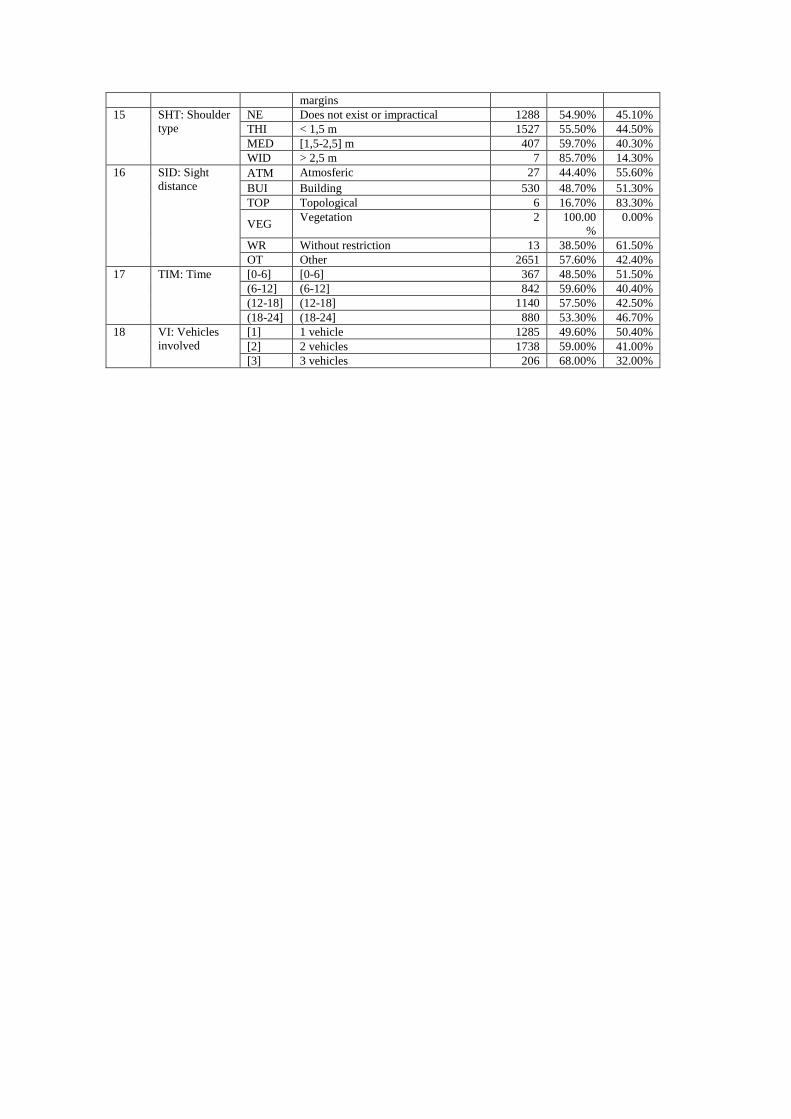
accident’s records used is 3,229. Table 1 provides information on the data used for this study.

(Table 1)

Considering that the main objective of this study is to identify the key factors that affect the

severity of traffic accidents, 18 explanatory variables based on De Oña et al. (2011) were used,

and injury severity was considered a class variable, with two classes: slightly injured (SI), or

killed or severely injured (KSI).

The data included variables describing the conditions that contributed to the accident and injury

severity: characteristics of the accident (month, time, day type, number of injuries, number of

occupants, accident type, number of involved vehicles and cause); weather information

(prevailing weather conditions and lighting); driver characteristics (age and gender); and road

characteristics (pavement width, lane width, shoulder width, paved shoulder, pavement

markings and sight distance).

6

4. RESULTS AND DISCUSSION

4.1. Cluster analysis

Latent GOLD software (v.4.0) was used for LCC analysis. Table 1 shows the 18 variables used,

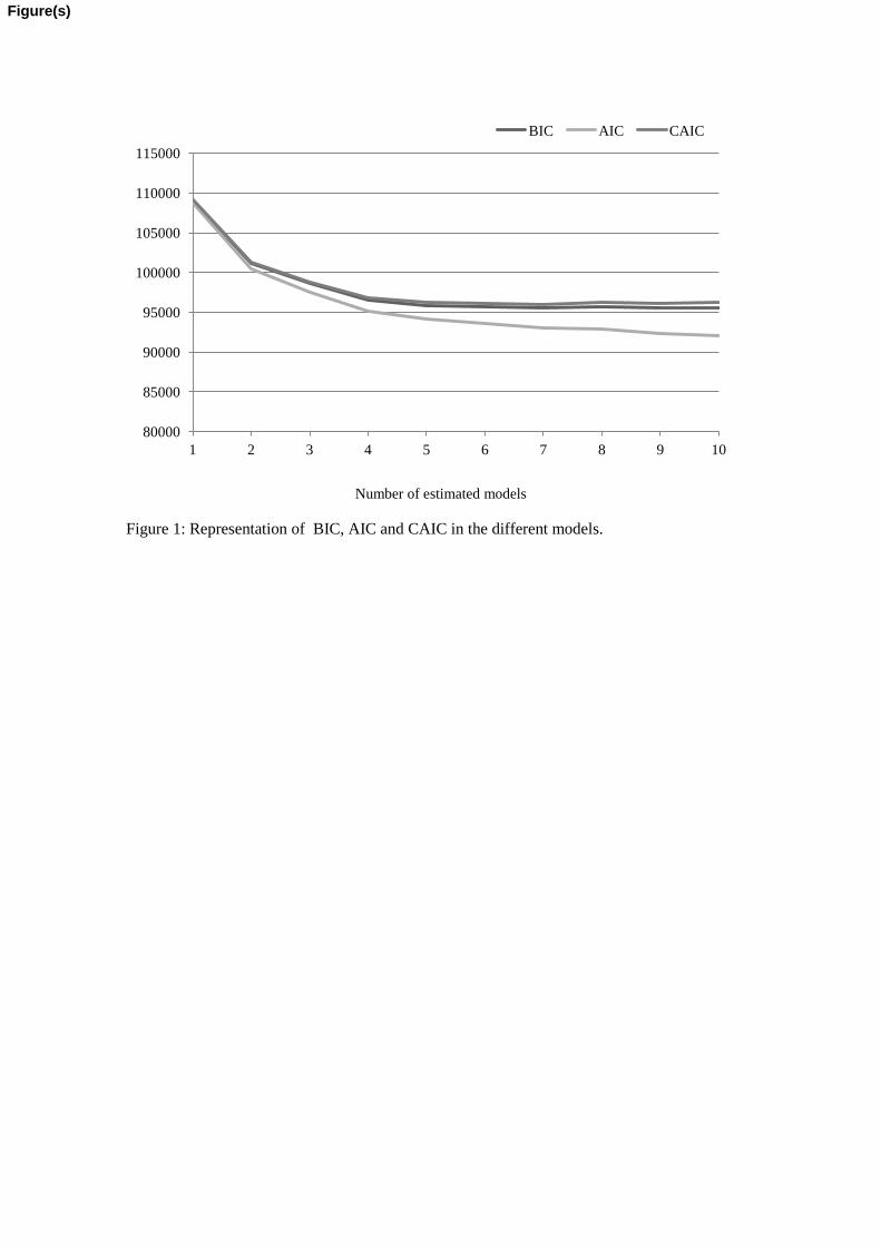
with injury severity as a dependent variable. In order to select the number of clusters, 10 models

were generated (from one to 10 clusters). Figure 1 shows the evolution of BIC, AIC and CAIC

for the 10 models. Increasing the number of clusters reduces BIC, AIC and CAIC values, but a

higher degree of clusters implies a higher degree of complexity, leading to a less obvious

clustering structure, despite a better statistical fit.

From a practical point of view, it is no so useful to have a marginal improvement in statistical

fit, but a higher degree of complexity. So, as a tradeoff between statistical fit and complexity of

clustering structure the model selected is the one with 4 clusters. In any case, this selection is in

accordance with the literature: Depaire et al. (2008) selected the model where BIC and CAIC

hardly show any additional improvement; Scheire et al. (2008) chose a model in which the

differences attained are less than 1%; In addition, the entropy for model 4 is 0.9873, which

indicates a good separation between clusters (McLachlan and Peel, 2000).

(Figure 1)

Having ascertained the number of clusters, the next step consisted in characterizing them. To

that end, it was necessary to identify the most important categories within each cluster for each

variable (using for that the highest conditional probability obtained for a determined category of

a variable given its membership to a specific cluster).

Therefore, the characterization was based on utilizing the variables that permitted differentiation

between clusters. Having performed the analysis, it was found that not all the variables could be

used for the established target for the following reasons:

- The highest value of probability was obtained for the same category of a specific

variable in all of the clusters built. This occurs in the variables time (TIM), number of

injuries (NOI), cause (CAU), atmospheric factors (ATF), lighting (LIG), age (AGE),

pavement markings (ROM) and sight distance (SID). For example, in the case of the

variable TIM, the highest probability of having an accident at each of the 4 target

clusters of the study is obtained in the same time period (12-18]. It should be noticed

that although this variable does not permit a characterisation of the clusters, it permits

knowing that the highest probability of accidents occurs during this time period.

- The probability values are distributed homogeneously between every possible category

of a variable; and therefore it does not permit clusters’ characterization. This occurs in

the variables month (MON) and day (DAY) (i.e. in cluster 1, the probability for each

category of MON (Winter, Spring, Summer and Autumn) are 24.82%, 23.15%, 26.48%

and 25.55%, respectively, and the same is true in clusters 2, 3 and 4. Thus, with these

results, it is not possible to say that an accident would have a higher probability of

occurrence in a specific season).

Finally, Table 2 shows the five variables selected to characterise the clusters, along with their

probability in each one of the 4 clusters identified.

(Table 2)

CLUSTER 1 (C1). It includes 100% of the accidents with 2 occupants or more, which occur on

highways with a shoulder that is less than 1.5 m in 77% of the cases and is a paved shoulder in

almost 100% of the cases. The collisions (with 94% of probability) are the type of accident that

characterize C1, highlighting angle or side collisions (54%); in 88% of the cases 2 vehicles were

7

involved in the accident. Thus, based on these characteristics, C1 could be called: “Collisions on

highways with shoulder”.

CLUSTER 2 (C2). It includes 67% of the accidents in which only one occupant was involved,

and which occur on highways with a shoulder width of 1.5 m in 78% of the cases, and that have

a 99% probability of being paved. They are accidents that are caused by run-off-road

with/without collision (83%), in which one vehicle was involved with 99% of probability. C2

could be called: “Run-off-road accidents and collisions with pedestrians on highways with

shoulder”.

CLUSTER 3 (C3). It includes any accident with 2 occupants or more (0% of probability for 1

occupant); but with a deviance in cluster 1, these are produced on highways without a shoulder

or with an impractical shoulder (99%). The types of accident that characterize this cluster are

collisions (with 94% of probability). Based on these characteristics, it is observed that C1 and

C3 overlap. C3 could be called: “Collisions on highways with no shoulders”.

CLUSTER 4 (C4). This cluster contains 61% of the accidents with 1 occupant. They occur on

highways that have no shoulder (99%). The type of accident that characterizes them is the run-

off-road with/without collision (85%), and in 100% of the cases there is only one vehicle

involved. Once again it is observed that C2 and C4 overlap. C4 could be called: “Run-off-road

accidents and collisions with pedestrians on highways with no shoulders”.

The previous definitions and values in Table 2 show that the data in C1 and C3 are more

homogeneous that the data in C2 and C4. Table 3 shows the number of cases in each cluster that

ranges between 19% and 40% of the total sample size. C1 stands out with close to 1,300 cases,

whereas C2, C3 and C4 are similar in size, with 600-700 cases.

(table 3)

With the data used in this study, four different clusters were identified, based on accident type,

the number of vehicles and occupant involved, the shoulder type and the shoulder pavement. It

should be highlight that the descriptive cluster analysis in this paper is focused on getting a

concise description for each cluster, which will be useful during the interpretation of BN results.

4.2. Severity injury analysis

Bayesian Networks (BN) are used in order to identify the main factor that contribute to crash

severity. BN were built for the entire database (EDB) and for each one of the four clusters (C1,

C2, C3 and C4) identified with LCC. The objective is to verify if new information and insights

are obtained from the conjoint analysis (LCC and BN). First, the five BNs were compared in

terms of performance indicators and complexity in order to evaluate the goodness of the models

obtained. Next, the possibility of obtaining new information and insights from the clusters was

studied in terms of direct dependent relationships between the variables for each BN and an

analysis of the inference in the BNs for the clusters that improve the performance indicators,

compared to the EDB.

(Table 4)

Table 4 shows accuracy, sensitivity, specificity, ROC area and HMSS for the EDB and clusters

C1 to C4. ANOVA test was performed to measure the statistical significant difference for each

cluster as compared to the EDB (p<0.05). The values of accuracy range from 64.0% in C1 to

55.1% in C4. These values are within the same range found in previous studies (Abdelwahab

and Abdel-Aty, 2001; De Oña et al., 2011; Mujalli and De Oña, 2011) that used classification

techniques for similar objectives. Table 4 shows that only C1 (64.0%) achieved a statistically

significant improvement of accuracy as compared with results obtained for the EDB (59.5%).

8

C3 obtained similar accuracy results to these obtained in the EDB (58.9% versus 59.5%). The

minimum accuracy is obtained in C4, which is also the smallest cluster. With regard to

sensitivity, both C1 and C3 obtained significant improvements if compared to the EDB. The

same repeats for specificity and for HMSS. For ROC area, only C1 improves significantly

(67.0%) with respect to 63.0% obtained for the EDB.

Another factor to be taken into consideration is network complexity (number of arcs). All the

clusters' networks show a fewer number of arcs than the EDB (33 arcs): C2’s BN is the simplest

with 19 arcs; C1, C3 and C4 present 21 arcs.

On the basis of these results, LCC enabled the identification of two clusters (C1 and C3) where

the BN models' overall performance improved with regards to the EDB. This was not the case

for clusters C2 and C4, where the results were not as good as they were for C1 and C3, and they

did not improve the results obtained for the EDB’s BN model.

Subsequently, on the basis of the BNs built for the EDB and the 4 clusters, it was possible to

identify the direct dependence relationships between severity (SEV) and the dependant variables

considered in the analysis. Table 5 shows the direct relationships between variables that were

present either in the clusters or in the EDB. The clusters that share the same relationships are

listed under the same group; in which the group refers to the number of BN that share the same

relation (e.g. the relationship “time→lighting” (TIM→LIG) exists in the BNs built using all the

4 clusters as well as using the EDB, however, the relationship “severity→atmospheric factors”

(SEV→ATF) exists only in the 4 clusters).

(Table 5)

Table 5 shows that no direct relationship of dependency between severity (SEV) and lane with

(LAW) can be observed in any of the cases (neither the EDB nor the clusters). As indicated in

Section 2.2, this does not mean that no relationship between SEV and LAW exists; only that the

relationship is not direct. In this case, indirect dependence relationships exist through other

variables, such as pavement width (PAW) and pavement markings (ROM) in the EDB, C3 and

C4, or PAW in C1 and C2 (see Table 5).

Several variables, such as month (MON), time (TIM), day (DAY), number of injuries (NOI),

accident type (ACT), cause (CAU), age (AGE), gender (GEN), pavement width (PAW),

shoulder type (SHT), pavement markings (ROM) and sight distance (SID), present a direct

dependence relationship with severity (SEV) in all groups. The fact that they appear in all the

groups may indicate that these variables have a strong correlation with SEV. There are also

other three direct relations that appear in all groups: time→lighting (TIM→LIG); number of

injuries→occupants involved (NOI→OI); and pavement width→lane width (PAW→LAW). All

the results are coherent because the variables are highly correlated with each other.

However, the main reason for using LCC analysis prior to BNs is to identify relationships that

only occur in specific clusters and not in the EDB or in the other clusters. Table 5 shows

relationships identified in the clusters that are not identified when only the EDB is analysed.

The table shows that a direct dependence relationship between severity and number of vehicles

involved in the accident (SEV→VI) only exists in C2. Table 5 also shows a direct relationship

between severity and occupant involved (SEV→OI) only for EDB and C3. There are two direct

dependence relationships that appear in three groups: severity with paved shoulder

(SEV→PAS) is observed in C1, C2 and C4; and severity with lighting (SEV→LIG) is observed

in the EDB, C2 and C4. The direct relationship between severity and atmospheric factors

(SEV→ATF) is present in all the four clusters but not in the EDB.

It is also worth mentioning a series of direct dependence relationships between SEV and other

variables that have been identified in the clusters' BN but not in the EDB’s BN. These are:

9

- A direct link between SEV and atmospheric factors (ATF) is present in all the four clusters’

BNs but it is not present for the EDB. In this case, an indirect dependence relationship

exists through month (MON).

- A direct link between SEV and paved shoulder (PAS) is present in BNs of clusters C1, C2

and C4 but it is not present for the EDB. In this case, an indirect dependence relationship

exists through several variables: pavement width (PAW), pavement markings (ROM), sight

distance (SID) and shoulder type (SHT).

- A direct link between SEV and vehicles involved (VI) is present in C2’s BN but it is not

present for the EDB. In this case, an indirect dependence relationship exists through several

variables: accident type (ACT), age (AGE), gender (GEN), time (TIM), number of injuries

(NOI) and occupants involved (OI).

The preceding analysis allowed the identification of further relationships between variables for

certain types of accidents (clusters), which would not have been obtained without prior

segmentation of the data. However, we focus on BN inference to analyse the results from a road

safety perspective. Inference is used to determine the most significant variables that are

associated with KSI (killed or severely injured) accidents for the EDB, C1 and C3. The analysis

was not made for the BN models for C2 and C4 because their performance indicators were

poorer than the EDB’s BN model.

(Table 6)

Table 6 assists in the identification of variables and values that contribute the most to the

occurrence of a KSI individual in a traffic accident considering each one of the three BN models

(EDB, C1 and C3). Since it is intended to determine which values of variables contribute the

most to the occurrence of a KSI individual in a traffic accident, this table does not include the

variables and values in which the values of probabilities of SI are always higher than those of

KSI in the EDB, C1 and C3.

For each variable and each BN model, the probability of a value was set to be 1.0 (setting

evidence) and the other values of the same variable were set to be 0.0. Thus, the associated

probability of severity was calculated. Underlined values in Table 6 show the values of

variables in which the probability of a KSI was found to be higher than that of SI.

For the EDB, Table 6 shows that assigning a probability of 1.0 to the value CP (collision with

pedestrian) of the variable accident type (ACT), the probability of SI becomes 0.3316 and the

probability of KSI becomes 0.6683. These probabilities are calculated from the conditional

probability table of the BN built for the EDB.

Setting evidences for the values of variables used to build the BN indicated that accident type

(ACT), sight distance (SID), time (TIM), occupant involved (OI), age (AGE), and lighting

(LIG) were found to be significant for the EDB. This results are coherent with previous studies

which have highlighted some of this variables as key variables in KSI accidents (Abel-Aty

2003; Al-Ghamdi, 2002; de Oña et al., 2011; Gray et al., 2008; Helai et al., 2008; Kashani and

Mohyamany, 2011; Kockelman and Kweon, 2002; Pande and Abel-Aty, 2009; Montella et al.,

2011).

Setting evidences in the cluster’s BN models (C1 and C3) shows similarities and differences

with the EDB results (see Table 6). The main similarities are:

- Although the values change with regards to the EDB, the variables accident type (ACT) and

sight distance (SID) are also significant in the case of C1 and C3.

- EDB and C3 show very similar results when setting evidences for the values of time (TIM),

occupant involved (OI) and age (AGE).

10

Accident type (ACT) has been identified in several previous studies (Al-Ghamdi, 2002; de Oña

et al., 2011; Kashani and Mohyamany, 2011; Montella et al., in press) as one of the key

variables in accident severity. Particularly, in this study head-on collision (HOC) and collision

with pedestrian (CP) were the type of accident with the highest probability of KSI (see Table 6).

These results agree with Kockelman and Kweon (2002), who found that head on crashes were

more dangerous than angle crashes, left-side, and right-side crashes; moreover, they found that

they were significant in accidents that involved KSI. Chang and Wang (2006) demonstrated that

collisions with pedestrian had a higher risk of injury than other types of collision. And de Oña et

al., (2011) highlighted that head on collision and rollover were more significant in KSI

accidents.

Yan et al. (2008) found that drivers suffering from poor visibility are less likely to attempt to

avoid crashes. And Montella (2011) identified that an inadequate sight distance was a major

factor contributory in roundabout crashes. This study shows that if sight distance (SID) is

restricted by the topography (TOP) or buildings (BUI) the probability of KSI accident increases.

The number of occupants involved (NOI) in a traffic accident was found to be a significant

variable by Dupont et al. (2010). They found that the higher the number of vehicles involved in

an accident and the level of occupancy of these vehicles, the higher the probability for each car

occupant to survive. This agrees with our results in which the probability of KSI accident

increases if there is only one occupant involved.

In accordance with previous studies (Tavris et al., 2001; Mujalli and de Oña, 2011), our results

show that teenagers (TEE) have a higher probability of KSI accidents. Tavris et al. (2001) found

that young people between 16 and 24 years were much more likely to be involved in KSI

accidents than older drivers.

When lighting conditions (LIG) are without lighting (WL) the probability of KSI is higher. This

result was also found by Gray et al. (2008). They identified that more severe injuries are

predicted during darkness. Abel-Aty (2003) and Helai et al. (2008) found the same results.

Pande and Abel-Aty (2009) concluded that there is a significant correlation between lack of

illumination and high severity crashes. Finally, de Oña et al. (2010) also pointed out that KSI

accidents are associated with roadways without lighting. This study shows that accidents

between 0 and 6 hours have a significant probability of being KSI. Our results also show that

the variables time (TIM) and lighting conditions (LIG) are directly correlated (see Table 5).

The main differences found between the clusters and the EDB’s inference are the following (see

Table 6):

- The lighting variable (LIG) is not identified as significant in clusters C1 and C3.

- The variables time (TIM), occupants involved (OI) and age (AGE) are not identified as

significant in cluster C1, which refers to collision on highways with shoulders.

- The variable vehicles involved (VI), when only 1 vehicle is involved, is identified as

significant in KSI accidents in cluster C3. This cluster contains very few accidents with

only one vehicle involved; however all of them present KSI consequences.

- The variables number of injuries (NOI), atmospheric factors (ATF), pavement markings

(ROM) and pavement width (PAW) are only identified as significant in cluster C1.

5. CONCLUSIONS AND RECOMENDATIONS

This paper presents an analysis of traffic accident injury severity on rural highways conducted

with the combined use of LCC and BN. The study uses 3,229 traffic accidents’ records on rural

highways. It is based on the standard police reports used in Spain, with information about 18

variables related with the injury severity of the accidents.

11

LCC analysis identified four clusters (C1 to C4) based on the variables accident type, shoulder

type, paved shoulder, occupant involved and number of vehicle involved. The main differences

in cluster identification are accident type (collisions or run-off road), and the existence of paved

shoulders on highways. Therefore, the conclusion is that the two variables are important in

accident analyses.

BNs were built for each one of the four clusters and for the entire database (EDB). Accuracy,

sensitivity, specificity, ROC area and HMSS were used as indicators for comparing model

fitting (EDB’s BN vs. the clusters’ BN). The models of clusters C1 and C3 (which showed the

highest homogeneity) show global results that are identical to or better than the model using the

EDB. Therefore, the results show that increasing homogeneity improves the models' overall

fitting.

The results were compared with the BN that uses the EDB and the BNs generated for each

cluster in terms of: direct dependence relationships between severity (SEV) and all the others

variables for EDB and for all the clusters; and inference for EDB and for the two clusters that

improved the performance indicators with regards to the EDB (C1 and C3). This comparison

has provided information and insights from the analysis that would not have been obtained if

only the EDB had been analysed, without making a LCC analysis beforehand.

For instance, it can be seen that a set of variables (month, time, day, number of injuries, accident

type, cause, age, gender, pavement width, shoulder type, pavement markings and sight distance)

show direct dependence relationships with severity both in the EDB and in all the clusters. This

implies that those variables are highly correlated with crash severity. On the other hand, no

direct link is observed between severity and atmospheric factors in the case of the EDB,

whereas a relationship does exist in all the clusters identifed, highlighting the important

relationship between this two variables, which has been also identify in previous studies

(Mujalli and De Oña, 2011; Xie et al., 2009).

The results from inference analysis identify several variables that have an influence on KSI

accidents. They are identified by EDB, and by C1 and C3. These variables are accident type

(ACT) and sight distance (SID). In all three cases (EDB, C1 and C3), when a collision with

pedestrians (CP) occurs on rural highways, the probability of KSI is very high (0.6663 - 0.8747,

in Table 6). Therefore, when pedestrians are frequent on such highways (i.e. on roads that link

two villages that are close to each other) it is advisable to take precautions against such

accidents (e.g. use of safety barriers on stretches of road where pedestrians walk on the

shoulder). In the three cases it is also observed that when the SID is very restricted by

topography (TOP), the probability of KSI is very high (0.6243 - 0.7497, in Table 6). Horizontal

and vertical traffic signs generally take limited visibility into account (e.g. signals for overtaking

other vehicles). However, the results also reveal that when SID is restricted by buildings (BUI),

the probability of KSI is very high for EDB and C1. Therefore, it would be advisable to take

limited visibility into account on rural highways, and to reassess visibility where there are

buildings are close to the road.

Inference also shows that certain variables that have not been identified as significant with the

EDB’s BN in determining whether or not an accident could be KSI, are identified as significant

for a specific cluster. For example, in cluster C3 if there is only one vehicle involved in a

collision (i.e. fixed object collision, run-off-road collision, or collision with pedestrian) the

probability of KSI is higher than the probability of SI. In cluster C1, the variables number of

injuries, atmospheric factors, pavement markings and pavement width are found to have a

significant impact on the probability of KSI. Taking into account these results, specific road

safety improvements could be applied. For example, in order to reduce the severity of collisions

on highways with shoulders (cluster C1), road markings should be repainted and signs of

narrow lanes should be used when road markings do not exist or are deleted or when pavement

12

width is less than 6 meters. None of these results would have been obtained if only the EDB had

been analysed, with no prior LCC analysis.

This study shows that the combined use of both methods (LCC and BNs) provide new

information and insights on the main causes of accident severity that could be useful for road

safety analysts. Therefore, this study agrees with previous research (Sohn, 1999; Karlaftis and

Tarko, 1998; Ng et al., 2002; Wong et al., 2004; Depaire et al., 2008; Pardillo-Mayora et al.,

2010) and shows that when analysing traffic accidents, it is worthwhile to segment the accident

records to increase data homogeneity before applying other analysis techniques.

Several considerations should be kept in mind when interpreting and generalizing the results of

this study. The results obtained in this paper are very dependent on the initial data (two lane

highways accidents with 1, 2 or 3 vehicles involved) and by the methods used (Latent Class

Clustering and Bayesian Networks). Different results might have been obtained if other analysis

data and methods had been used. All clustering techniques are very sensitive to the possibility

of finding a local maximum instead of a global maximum. In this regard, the solution found is

dependent on the initial parameter values. To prevent ending up with a local solution, the Latent

GOLD program uses 10 sets of random start values (Vermunt and Magidson, 2005). Bayesian

Networks need large datasets. The number of cases in EDB and C1 are comparable with

previous studies (De Oña et al., 2011; Mujalli and De Oña, 2011). However, because of the

clustering procedure, C2, C3 and C4 present a limited number of cases. Therefore, BN results

for these three clusters should be interpreted carefully.

ACKNOWLEDGEMENTS

The authors are grateful to the Spanish General Directorate of Traffic (DGT) for providing the

data necessary for this research. Griselda López wishes to express her acknowledgement to the

regional ministry of Economy, Innovation and Science of the regional government of Andalusia

(Spain) for their scholarship to train teachers and researchers in Deficit Areas, which has made

this work possible. The authors also appreciate the reviewer´s comments and effort in order to

improve the paper.

REFERENCES

Abdelwahab, H.T., Abdel-Aty, M.A. 2001. Development of Artificial Neural Network Models

to Predict Driver Injury Severity in Traffic Accidents at Signalized Intersections. Transportation

Research Record, 1746, 6–13.

Abdel-Aty, M. 2003. Analysis of driver injury severity levels at multiple locations using

ordered probit models. Journal of Safety Research 34, 597–603.

Acid, S., de Campos, L.M., Fernández-Luna, J.M., Rodríguez, S., Salcedo, J.L. 2004. A

comparison of Learning algorithms for Bayesian networks: a case study based on data from an

emergency medical service. Artificial Intelligence in Medicine, 30, 215–232.

Akaike, H. 1987. Factor analysis and AIC. Psychometrika, 52, 317-332.

Al-Ghamdi, A. 2002. Using logistic regression to estimate the influence of accident factors on

accident severity. Accident Analysis and Prevention 34 (6), 729–741.

Biernacki, C., Govaert, G. 1999. Choosing models in model-based clustering and discriminant

analysis. J. Statis. Comput. Simul. 64, 49-71.

Bijmolt, T.H., Paas, L.J., Vermunt, J.K. 2004. Country and Consumer Segmentation: Multi-

level Latent Class Analysis of Financial Product Ownership. International Journal of Research

in Marketing, 21, 323-340.

13

Bock, H. 1996. Probabilistic models in cluster analysis. Computational Statistics and Data

Analysis 23 (1), 5-28.

Chang, L.Y., Wang, H.W. 2006. Analysis of traffic injury severity: an application of non-

parametric classification tree techniques. Accident Analysis and Prevention 38, 1019–1027.

De Oña, J., Mujalli, R.O., Calvo, F.J. 2011. Analysis of traffic accident injury on Spanish rural

highways using Bayesian networks. Accident Analysis and Prevention 43, 402–411.

Depaire, B., Wets, G., Vanhoof, K. 2008. Traffic accident segmentation by means of latent class

clustering. Accident Analysis and Prevention 40 (4), 1257–1266.

Dupont, E., Martensen, H., Papadimitriou, E., Yannis, G. 2010. Risk and Protection factors in

fatal accidents. Accident; Analysis and Prevention, 42, 645–653.

Fraley, C., Raftery, A.E. 1998. How Many clusters? Which Clustering Method? Answers via

Model-Based Cluster Analysis. The Computer Journal, 41, 578-588

Fraley, C., Raftery, A.E. 2002. Model-based clustering, Discriminant Analysis, and Density

Estimation. Journal of the American Statistical Association 97 (458), 611-631.

Gray, R.C., Quddus, M.A., Evans, A. 2008. Injury severity analysis of accidents involving

young male drivers in Great Britain. Journal of Safety Research 39, 483-495.

Hair, J.F.Jr., Anderson, R.E., Tatham, R.L., Black, W.C. 1998. Multivariate Data Analysis.

Prentice Hall.

Helai, H., Chor, C.H., Haque, M.M. 2008. Severity of driver injury and vehicle damage in

traffic crashes at intersections: a Bayesian hierarchical analysis. Accident Analysis and

Prevention 40, 45–54.

Karlaftis, M., Tarko, A. 1998. Heterogeneity considerations in accident modeling. Accident

Analysis and Prevention, 30(4), 425–433.

Kashani, A., Mohaymany, A. 2011. Analysis of the traffic injury severity on two-lane, two-way

rural roads based on classification tree models. Safety Science 49, 1314-1320.

Kockelman, K.M., Kweon, Y.J. 2002. Driver injury severity: an application of ordered probit

models. Accident Analysis and Prevention 34, 313–321.

Lord, D., Mannering, F. 2010. The statistical analysis of crash-frequency data: A review and

assessment of methodological alternatives. Transportation Research Part A, 44(5), 291-305.

Ma, J., Kockelman, K. 2006. Crash Frecuency and Severity Modeling Using Clustered Data

from Washintong State. IEEE Intelligent Transportation Systems Conference. Toronto, Canadá.

Magidson, J. and Vermunt, J.K. 2002. “Latent Class Models for clustering: a comparison with

K-means”, Canadian Journal of Marketing Research, 20, pp. 37-44.

Moustaki, I., Papageorgiou, I. 2005. Latent class models for mixed variables with applications

in Archaeometry. Computational Statistics and Data Analysis 48 (3), 659-675.

14

Madden, M.G. 2009. On the classification performance of TAN and general Bayesian networks.

Journal of Knowledge-Based Systems 22, 489–495.

McLachlan, G.J. and Peel, D. 2000. Finite Mixture Models. Wiley, New York.

Mittal, A., Kassim, A., Tan, T. 2007. Bayesian Network Technologies: Applications and

Graphical Models. IGI Publishing, New York.

Montella, A., 2011. Identifying crash contributory factors at urban roundabouts and using

association rules to explore their relationships to different crash types. Accident Analysis and

Prevention, 43(4), 1451-1463.

Montella, A., Aria, M., D´Ambrosio, A., Mauriello, F., 2011. Data Mining Techniques for

Exploratory Analysis of Pedestrian Crashes. Transportation Research Record 2237, 107-116.

Montella, A., Aria, M., D´Ambrosio, A., Mauriello, F., in press. Analysis of powered two-

wheeler crashes in Italy by classification trees and rules discovery. Accident Analysis and

Prevention, doi:10.1016/j.aap.2011.04.025

Mujalli, R.O. and De Oña, J. 2011. A method for simplifying the analysis of traffic accidents

injury severity on two-lane highways using Bayesian networks. Journal of Safety Research, 42,

317–326

Mujalli, R.O., De Oña, J. in press. Injury Severity Models for Motorized Vehicle Accident: A

review. Proceedings of the Institution of Civil Engineers – Transport, doi:10.1680/tran.11.00026

Neapolitan, R. E. 2004. Learning Bayesian Networks. Upper Saddle River, NJ: Prentice Hall.

Ng, K.S., Hung, W.T. and Wong, W.G. 2002. An algorithm for assessing the risk of traffic

accident. Journal of Safety Research 33, 387-410.

Pande, A., Abdel-Aty, M. 2009. Market basket analysis of crash data from large jurisdictions

and its potential as a decision supporting tool. Safety Science 47, 145–154.

Pardillo-Mayora, J.M., Domínguez-Lira, C.A., Jurado-Piña, R. 2010. Empirical calibration of a

roadside hazardousness index for Spanish two-lane rural roads. Accident Analysis and

Prevention 42, 2018-2023.

Park, B.-J., Lord, D. 2009. Application of finite mixture models for vehicle crash data analysis.

Accident Analysis and Prevention 41, 683–691.

Park, B.-J., Lord, D., Hart, J. 2010. Bias Properties of Bayesian Statistics in Finiture Mixture of

Negative Regression Models for crash data analysis. Accident Analysis and Prevention 42, 741–

749.

Raftery, A.E. 1986. A note on Bayes factors for log-linear contingency table models with vague

prior information. Journal of the Royal Statistical Society, series B, 48, 249-250.

Savolainen, P., Mannering, F., Lord, D., Quddus, M. 2011. The statistical analysis of highway

crash-injury severities: A review and assessment of methodological alternatives. Accident

Analysis and Prevention 43, 1666-1676.

Scheier, L.M., Abdallah, A.B. Iniardi J.A., Copeland, J., Cottler, L.B. 2008. Tri-city study of

Ecstasy use problems: A latent class analysis. Drug and Alcohol Dependence 98, 249-263.

15

Sepúlveda, R.A. 2004. Contribuciones al Análisis de Clases latentes en Presencia de

Dependencia Local. Tesis Doctoral, Universidad de Salamanca.

Simoncic, M. 2004. A Bayesian network model of two-car accidents. Journal of transportation

and Statistics, 7, 13–25.

Sohn, S.Y. 1999. Quality function deployment applied to local traffic accident reduction.

Accident Analysis and Prevention 31, 751–761.

Tavris, D.R., Kuhn, E.M., Layde, P.M., 2001. Age and gender patterns in motor vehicle crash

injuries: importance of type of crash and occupant role. Accident Analysis and Prevention 33,

167–172.

Vermunt, J.K., Magidson, J. 2002. Latent class cluster analysis. J.A. Hagenaars and A-L.

McCutcheon (eds). Applied latent class analysis, Cambridge: Cambridge University Press. 89-

106.

Vermunt, J.K., Magidson, J. 2005. Latent GOLD 4.0 User's Guide. Belmont, Massachusetts:

Statistical Innovations Inc."

Wong, S.C., Leung, B.S.Y., Loo, B. P.Y., Hung W.T. and Lo, H.K. 2004. A qualitative

assesment methodology for road safety policy strategies. Accident Analysis and Prevention 36,

281–293.

Xie, Y., Zhang, Y., Liang, F. 2009. Crash Injury Severity Analysis Using Bayesian Ordered

Probit Models. Journal of Transportation Engineering ASCE, 135(1), 18–25.

Yan X, Harb R, Radwan E. 2008 Analyses of Factors of Crash Avoidance Maneuvers Using the

General Estimates System. Traffic Injury Prevention, 9, 173–180.

16

List of figures:

Figure 1: Representation of BIC, AIC and CAIC in the different models.

List of tables:

Table 1. Variables, values and actual classification by severity

Table 2. Variables, categories and probabilities of membership to each cluster

Table 3. Definition of the clusters

Table 4. Results of the Bayesian Network in the clusters and OB

Table 5. Relations between variables in the Bayesian networks

Table 6. Inference results for variables that are associated with KSI in traffic accidents for EDB,

C1 and C3.

Number of estimated models

Figure 1: Representation of BIC, AIC and CAIC in the different models.

80000

85000

90000

95000

100000

105000

110000

115000

1 2 3 4 5 6 7 8 9 10

BIC AIC CAIC

Figure(s)

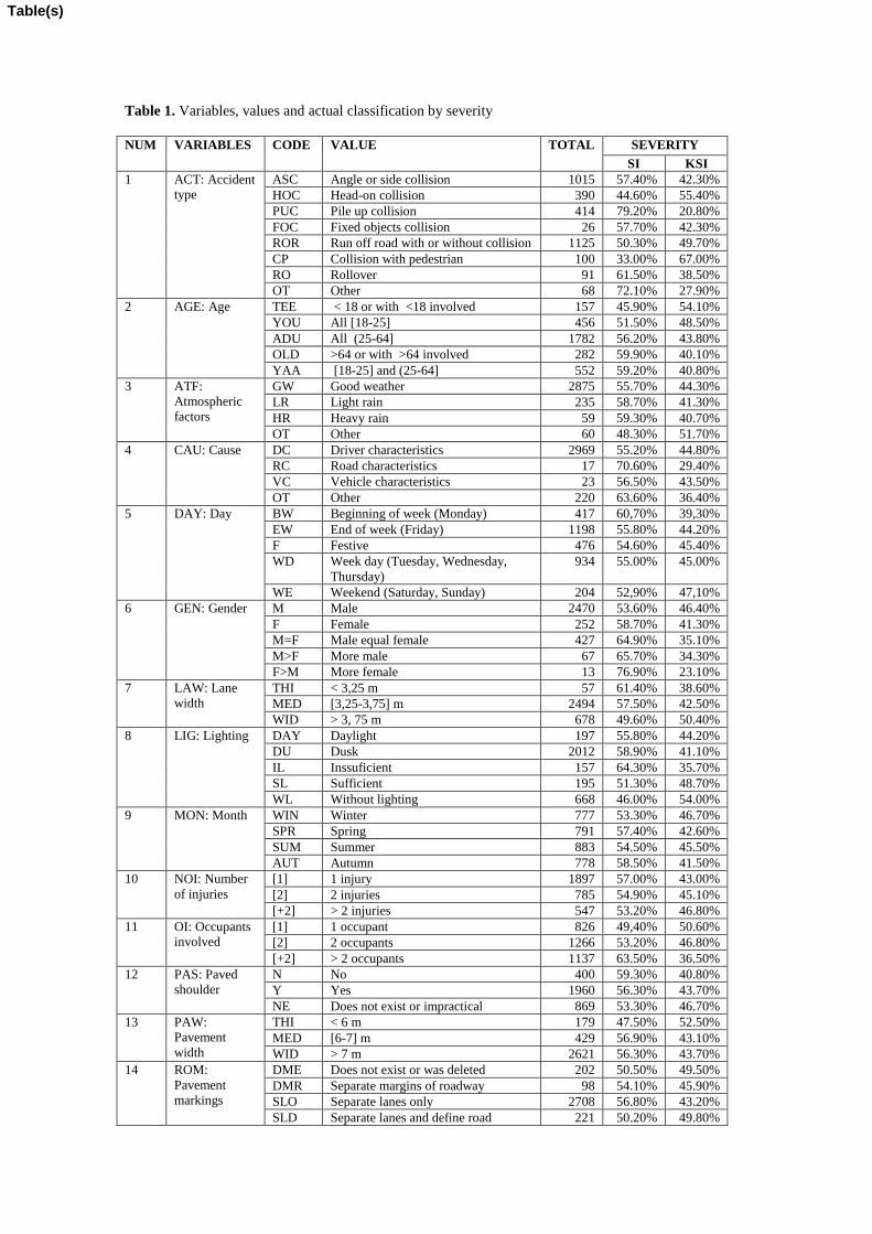
Table 1. Variables, values and actual classification by severity

NUM VARIABLES CODE VALUE TOTAL SEVERITY

SI KSI

1 ACT: Accident

type

ASC Angle or side collision 1015 57.40% 42.30%

HOC Head-on collision 390 44.60% 55.40%

PUC Pile up collision 414 79.20% 20.80%

FOC Fixed objects collision 26 57.70% 42.30%

ROR Run off road with or without collision 1125 50.30% 49.70%

CP Collision with pedestrian 100 33.00% 67.00%

RO Rollover 91 61.50% 38.50%

OT Other 68 72.10% 27.90%

2 AGE: Age TEE < 18 or with <18 involved 157 45.90% 54.10%

YOU All [18-25] 456 51.50% 48.50%

ADU All (25-64] 1782 56.20% 43.80%

OLD >64 or with >64 involved 282 59.90% 40.10%

YAA [18-25] and (25-64] 552 59.20% 40.80%

3 ATF:

Atmospheric

factors

GW Good weather 2875 55.70% 44.30%

LR Light rain 235 58.70% 41.30%

HR Heavy rain 59 59.30% 40.70%

OT Other 60 48.30% 51.70%

4 CAU: Cause DC Driver characteristics 2969 55.20% 44.80%

RC Road characteristics 17 70.60% 29.40%

VC Vehicle characteristics 23 56.50% 43.50%

OT Other 220 63.60% 36.40%

5 DAY: Day

BW Beginning of week (Monday) 417 60,70% 39,30%

EW End of week (Friday) 1198 55.80% 44.20%

F Festive 476 54.60% 45.40%

WD Week day (Tuesday, Wednesday,

Thursday)

934 55.00% 45.00%

WE Weekend (Saturday, Sunday) 204 52,90% 47,10%

6 GEN: Gender M Male 2470 53.60% 46.40%

F Female 252 58.70% 41.30%

M=F Male equal female 427 64.90% 35.10%

M>F More male 67 65.70% 34.30%

F>M More female 13 76.90% 23.10%

7 LAW: Lane

width

THI < 3,25 m 57 61.40% 38.60%

MED [3,25-3,75] m 2494 57.50% 42.50%

WID > 3, 75 m 678 49.60% 50.40%

8 LIG: Lighting DAY Daylight 197 55.80% 44.20%

DU Dusk 2012 58.90% 41.10%

IL Inssuficient 157 64.30% 35.70%

SL Sufficient 195 51.30% 48.70%

WL Without lighting 668 46.00% 54.00%

9 MON: Month WIN Winter 777 53.30% 46.70%

SPR Spring 791 57.40% 42.60%

SUM Summer 883 54.50% 45.50%

AUT Autumn 778 58.50% 41.50%

10 NOI: Number

of injuries

[1] 1 injury 1897 57.00% 43.00%

[2] 2 injuries 785 54.90% 45.10%

[+2] > 2 injuries 547 53.20% 46.80%

11 OI: Occupants

involved

[1] 1 occupant 826 49,40% 50.60%

[2] 2 occupants 1266 53.20% 46.80%

[+2] > 2 occupants 1137 63.50% 36.50%

12 PAS: Paved

shoulder

N No 400 59.30% 40.80%

Y Yes 1960 56.30% 43.70%

NE Does not exist or impractical 869 53.30% 46.70%

13 PAW:

Pavement

width

THI < 6 m 179 47.50% 52.50%

MED [6-7] m 429 56.90% 43.10%

WID > 7 m 2621 56.30% 43.70%

14 ROM:

Pavement

markings

DME Does not exist or was deleted 202 50.50% 49.50%

DMR Separate margins of roadway 98 54.10% 45.90%

SLO Separate lanes only 2708 56.80% 43.20%

SLD Separate lanes and define road 221 50.20% 49.80%

Table(s)

margins

15 SHT: Shoulder

type

NE Does not exist or impractical 1288 54.90% 45.10%

THI < 1,5 m 1527 55.50% 44.50%

MED [1,5-2,5] m 407 59.70% 40.30%

WID > 2,5 m 7 85.70% 14.30%

16 SID: Sight

distance ATM Atmosferic 27 44.40% 55.60%

BUI Building 530 48.70% 51.30%

TOP Topological 6 16.70% 83.30%

VEG Vegetation 2 100.00

%

0.00%

WR Without restriction 13 38.50% 61.50%

OT Other 2651 57.60% 42.40%

17 TIM: Time [0-6] [0-6] 367 48.50% 51.50%

(6-12] (6-12] 842 59.60% 40.40%

(12-18] (12-18] 1140 57.50% 42.50%

(18-24] (18-24] 880 53.30% 46.70%

18 VI: Vehicles

involved

[1] 1 vehicle 1285 49.60% 50.40%

[2] 2 vehicles 1738 59.00% 41.00%

[3] 3 vehicles 206 68.00% 32.00%

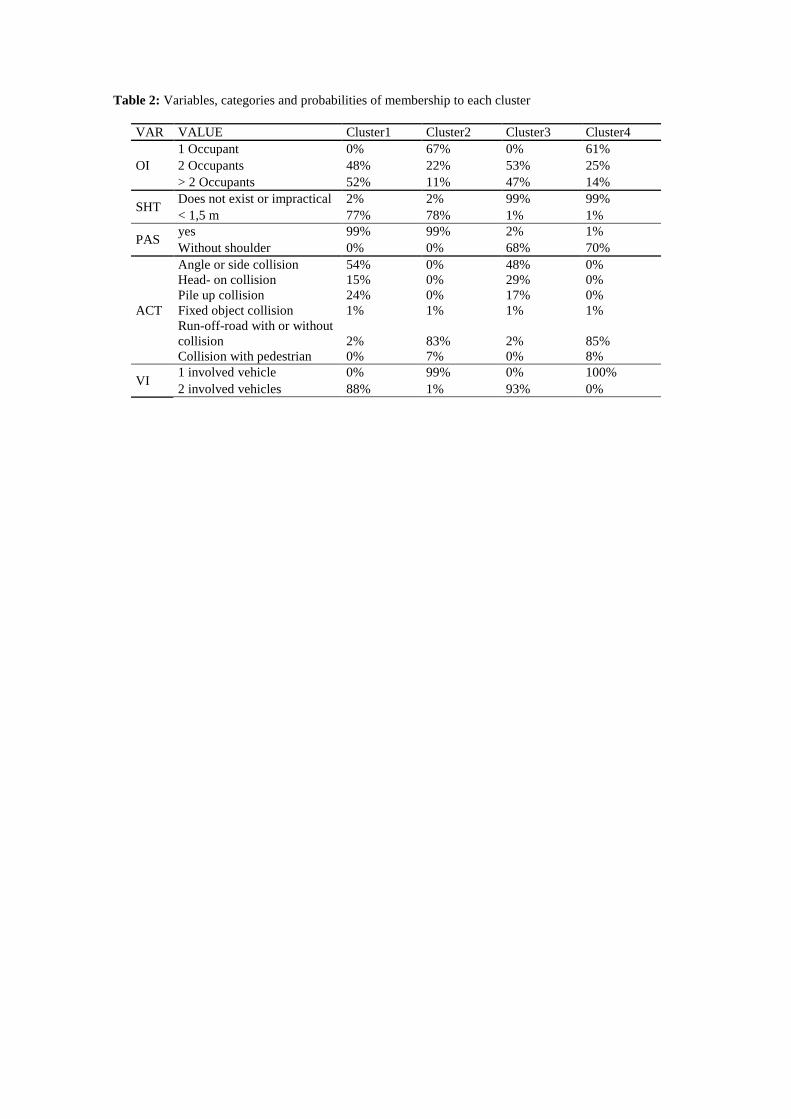
Table 2: Variables, categories and probabilities of membership to each cluster

VAR VALUE Cluster1 Cluster2 Cluster3 Cluster4

OI

1 Occupant 0% 67% 0% 61%

2 Occupants 48% 22% 53% 25%

> 2 Occupants 52% 11% 47% 14%

SHT Does not exist or impractical 2% 2% 99% 99%

< 1,5 m 77% 78% 1% 1%

PAS yes 99% 99% 2% 1%

Without shoulder 0% 0% 68% 70%

ACT

Angle or side collision 54% 0% 48% 0%

Head- on collision 15% 0% 29% 0%

Pile up collision 24% 0% 17% 0%

Fixed object collision 1% 1% 1% 1%

Run-off-road with or without

collision 2% 83% 2% 85%

Collision with pedestrian 0% 7% 0% 8%

VI 1 involved vehicle 0% 99% 0% 100%

2 involved vehicles 88% 1% 93% 0%

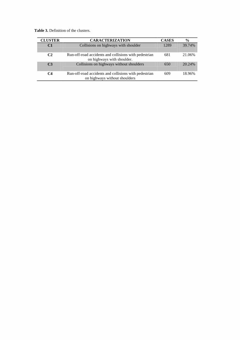
Table 3. Definition of the clusters.

CLUSTER CARACTERIZATION CASES %

C1 Collisions on highways with shoulder 1289 39.74%

C2 Run-off-road accidents and collisions with pedestrian

on highways with shoulder.

681 21.06%

C3 Collisions on highways without shoulders 650 20.24%

C4 Run-off-road accidents and collisions with pedestrian

on highways without shoulders

609 18.96%

Table 4. Results of the Bayesian Network in the clusters and OB.

Subset Accuracy Sensitivity Specificity ROC Area HMSS

C1 64.0* 78.0* 56.0* 67.0* 65.0*

C2 58.0 61.0 45.0 61.0 51.0

C3 58.9 78.0* 71.0* 57.0 74.0*

C4 55.1 47.0 37.0 56.0 41.0

EB 59.5 69.0 52.0 63.0 59.0

* denotes differences statistically significant (p < 0.05)

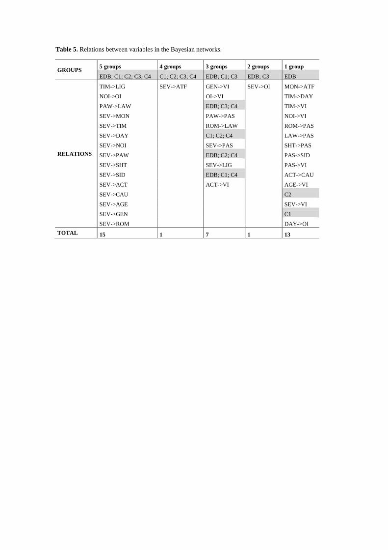
Table 5. Relations between variables in the Bayesian networks.

GROUPS 5 groups 4 groups 3 groups 2 groups 1 group

EDB; C1; C2; C3; C4 C1; C2; C3; C4 EDB; C1; C3 EDB; C3 EDB

RELATIONS

TIM->LIG SEV->ATF GEN->VI SEV->OI MON->ATF

NOI->OI

OI->VI

TIM->DAY

PAW->LAW

EDB; C3; C4

TIM->VI

SEV->MON

PAW->PAS

NOI->VI

SEV->TIM

ROM->LAW

ROM->PAS

SEV->DAY

C1; C2; C4

LAW->PAS

SEV->NOI

SEV->PAS

SHT->PAS

SEV->PAW

EDB; C2; C4

PAS->SID

SEV->SHT

SEV->LIG

PAS->VI

SEV->SID

EDB; C1; C4

ACT->CAU

SEV->ACT

ACT->VI

AGE->VI

SEV->CAU

C2

SEV->AGE

SEV->VI

SEV->GEN

C1

SEV->ROM

DAY->OI

TOTAL 15 1 7 1 13

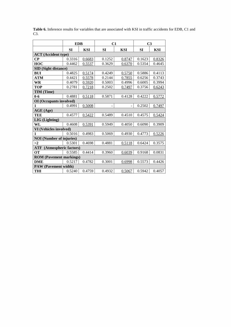
Table 6. Inference results for variables that are associated with KSI in traffic accidents for EDB, C1 and

C3.

EDB C1 C3

SI KSI SI KSI SI KSI

ACT (Accident type)

CP 0.3316 0.6683 0.1252 0.8747 0.1623 0.8326

HOC 0.4462 0.5537 0.3629 0.6370 0.5354 0.4645

SID (Sight distance)

BUI 0.4825 0.5174 0.4249 0.5750 0.5886 0.4113

ATM 0.4421 0.5578 0.2144 0.7855 0.6256 0.3743

WR 0.4079 0.5920 0.5003 0.4996 0.6005 0.3994

TOP 0.2781 0.7218 0.2502 0.7497 0.3756 0.6243

TIM (Time)

0-6 0.4881 0.5118 0.5871 0.4128 0.4222 0.5772

OI (Occupants involved)

1 0.4991 0.5008 - - 0.2502 0.7497

AGE (Age)

TEE 0.4577 0.5422 0.5489 0.4510 0.4575 0.5424

LIG (Lighting)

WL 0.4608 0.5391 0.5949 0.4050 0.6090 0.3909

VI (Vehicles involved)

1 0.5016 0.4983 0.5069 0.4930 0.4773 0.5226

NOI (Number of injuries)

>2 0.5301 0.4698 0.4881 0.5118 0.6424 0.3575

ATF (Atmospheric factors)

OT 0.5585 0.4414 0.3960 0.6039 0.9168 0.0831

ROM (Pavement markings)

DME 0.5217 0.4782 0.3001 0.6998 0.5573 0.4426

PAW (Pavement width)

THI 0.5240 0.4759 0.4932 0.5067 0.5942 0.4057