analysis of time-varying cellular neural networks for quadratic global optimization

INTERNATIONAL JOURNAL OF CIRCUIT THEORY AND APPLICATIONSInt. J. Circ. Theor. Appl., 26, 109–126 (1998)

ANALYSIS OF TIME-VARYING CELLULAR NEURAL NETWORKSFOR QUADRATIC GLOBAL OPTIMIZATION

M. GILLI∗1, P. P. CIVALLERI1, T. ROSKA2, AND L. O. CHUA3

1Cattedra di Elettrotecnica, Dipartimento di Elettronica, Politecnico di Torino, Caso Dua degli Abruzzi 24, I-10129 Torino, Italy2Computer and Automation Institute, Hungarian Academy of Sciences

3Department of Electrical Engineering and Computer Sciences, University of California, Berkeley, U.S.A.

SUMMARY

The algorithm for quadratic global optimization performed by a cellular neural network (CNN) with a slowly varyingslope of the output characteristic (see References 1 and 2) is analysed. It is shown that the only CNN which �nds theglobal minimum of a quadratic function for any values of the input parameters is the network composed by only two cells.If the dimension is higher than two, even the CNN described by the simplest one-dimensional space-invariant templateA= [A1; A0; A1], fails to �nd the global minimum in a subset of the parameter space. Extensive simulations show thatthe CNN described by the above three-element template works correctly within several parameter ranges; however, if theparameters are chosen according to a random algorithm, the error rate increases with the number of cells. c© 1998 JohnWiley & Sons, Ltd.

1. INTRODUCTION

There are several scienti�c and technological problems that can be reduced to the global optimization ofa quadratic function over a polyhedron.3 For the solution of these problems, exact algorithms which arepolynomial in the size of the problem (i.e. polynomial-time algorithms) have been found only in someparticular cases.4 Most quadratic optimization problems belongs to the class of NP-complete (non-deterministicpolynomial-time complete) problems,5 for which no polynomial-time exact algorithms are known. Severalapproximate and heuristic polynomial-time algorithms for such problems have been proposed3; 6 but theirimplementation on a fast parallel computer appears to be quite di�cult.7

Recently, new approaches, based on arti�cial neural networks and on stochastic optimization techniques (likesimulated annealing and Boltzmann machine7; 8) have been successfully exploited for solving some quadraticoptimization problems in real time. However such tecniques give rise to stochastic algorithms that do notalways converge to the optimal solution and that sometimes do not even converge to a good solution (i.e. anear-optimal solution). Some deterministic algorithms for quadratic global optimization, which exploit arti�cialneural networks, are summarized in Sections 9.2 and 9.3 of Reference 7. These algorithms try to avoid theconvergence to local minima, by gradually increasing the slope of the activation function of the network. Infully connected networks, such techniques often fail to �nd correclty the global minimum (see Reference 7).In References 1 and 2 a deterministic approach for quadratic global optimization which exploits time-varying

cellular neural networks (CNNs) has been proposed. This approach is still based on the gradual incrementof the slope of the CNN output function. However, owing to the fact that the CNN is described by a

∗Correspondence to: Dr M. Gilli, Cattedra di Elettrotecnica, Dipartimento di Elettronica, Politecnico di Torino, Caso Dua degli Abruzzi 24,I-10129 Tonno, Italy. Email: [email protected]

CCC 0098–9886/98/020109–18$17.50 Received 30 April 1996? 1998 John Wiley & Sons, Ltd. Revised 4 December 1996

110 M. GILLI ET AL.

space-invariant template, in References 1 and 2 the authors have observed the convergence to the globaloptimum in several interesting and important cases. Moreover, as pointed out in References 1 and 2, ahardware realization of the time-varying network is also possible.This paper is devoted to the theoretical investigation of time-varying CNNs with a slope of the output

function which is gradually increased from 0 to 1. The paper is organized as follows: in Section 2 we introducethe global optimization problem addressed by using the time-varying CNN; in Section 3 we describe howsuch a CNN works and which algorithm it performs; in Section 4 we discuss the correctness of the algorithmand �nally in Section 5 we draw some conclusions.

2. THE PROBLEM

The problem addressed by the time-varying CNN is the global minimization over a hypercube of the followingquadratic function:

E(y)=− 12 y

′(A− I)y − y′u; y∈Dn (1)

where A is a symmetric matrix, u is a constant vector of Rn, and Dn is the hypercube de�ned by Dn={y∈Rn; −16yi61; 16i6n}.Such a problem has been and is still widely studied in the literature (see Reference 3). Depending on the

symmetric matrix A the following particular cases may be considered:

(1) If A−I¡0 then the problem reduces to the global minimization over a polyhedron of a convex quadraticfunction and several exact algorithms have been proposed.3

(2) If A − I¿0 then the problem is equivalent to the global minimization of a concave function overa polyhedron (i.e. the hypercube); it is known that the global minimum occurs at one vertex of thehypercube.3 Moreover by substituting in (1) y=2x− 1, the problem is reduced to the minimization ofa concave quadratic function over the hypercube of vertices 0–1 and is known in the literature as thequadratic 0–1 problem. Such a problem has been shown to be NP-hard5 with respect to the number ofcomponents of the vector y and several approximate algorithms for solving it in a polynomial time havebeen proposed.6 Only in some particular cases exact polynomial-time algorithms have been found (see,for example, Reference 4 where the problem is solved under the assumption that the graph de�ned byA be series parallel). Moreover, we remark that the quadratic 0–1 optimization problem is equivalentto the max-cut problem in a weighted graph.4

(3) If the matrix A − I is neither positive nor negative, the problem, known as the inde�nite quadraticproblem, is very complex and no polynomial-time exact algorithms exist in the literature.3

3. TIME-VARYING CNNS FOR QUADRATIC GLOBAL OPTIMIZATION

In this section we study in detail the dynamics of CNNs whose output function slope is slowly increasedfrom 0 to 1 (i.e. the model proposed in References 1 and 2). In particular, we will show that, under someassumptions, the resulting time-varying CNN implements a new algorithm for the global optimization ofquadratic functions. Then we will discuss the validity and the correctness of such an algorithm.

3.1. The time-varying CNN

A time-varying CNN with a gradually increasing output function slope is described by the following equation(see References 1 and 2):

x=−x + Ay(g(t)x) + u (2)

Int. J. Circ. Theor. Appl., 26, 109–126 (1998) ? 1998 John Wiley & Sons, Ltd.

TIME-VARYING CELLULAR NETWORKS FOR OPTIMIZATION 111

where x is a vector representing the state of the network, u is the constant input and y(·) is the piecewiselinear saturation function, introduced in Reference 9:

y(w)= 12 (|w + 1| − |w − 1|) (3)

The term g(t) is a scalar monotone increasing function with the property that, for a small ”, 0¡”¡g(t)61.It is supposed that the CNN is described by a space-invariant template, from which matrix A is derived.

As a consequence all the diagonal entries of matrix A are equal; they will be denoted by A0.By substituting z= gx the above equation can be written as follows:

z=−z + g(t)Ay(z) + g(t)u+ g(t)g(t)

z (4)

If g is varied from ” to 1 in a su�ciently slow way, then the term |g(t)=g(t)|� 1 can be neglected;moreover, the dynamics of the network can be studied by considering g as the bifurcation parameter of thesystem described by the equation reported below:

z=−z + gAy(z) + gu (5)

We will denote each region of linearity of the CNN described by equation (5) by a sequence of 1’s, −1’sand X ’s according to the value of the ordered co-ordinates in the output (+1 means positive saturation, −1means negative saturation, X linear part of the characteristic for that variable).The following considerations hold:

1. For a value of g small enough (i.e. g= ”) it is easily seen by direct computation that the system (5)exhibits only one equilibrium point, close to zero and therefore belonging to the central region of theCNN (i.e. the region where all the cells work in the linear part of their characteristic). Such a pointis stable and its basin of attraction is the whole state space, i.e. each trajectory converges towards thatpoint.

2. By increasing g the position of such an equilibrium moves, describing a one-dimensional curve in Rn,that we will denote as z(g).Depending on matrix A− I we have two possibilities.(a) If A − I¡0, then by increasing g from ” to 1, the determinant of −I + gA is negative; therefore,

z(g) remains the only equilibrium point of system; since the matrix A is symmetric such a point isstable; it is concluded that from each initial condition system (4) converges towards z(1); since nonew equilibria appear it is easily shown that y(z(1)) is the global minimum of (1).

(b) If A− I is not negative de�nite, by increasing g from ” to 1, two situations may occur:i. Beyond z(g), new equilibria may appear, as a consequence of saddle-node bifurcations occurringat the border between some pairs of regions of linearity.

ii. It is not guaranteed that the equilibrium z(g) is stable for any g. A su�cient condition (denotedin the following as SC) for the stability of z(g) is that all the co-ordinates of z(g) which reacha saturation value ±1, for a given g, by increasing g do not come back to the linear part of theoutput characteristic. (The proof of this proposition is reported in Appendix I).

Depending on the stability of z(g) we have two possibilities:i. If z(g) is stable for any g∈ [”; 1], and the variation of g is su�ciently slow, then even in thiscase for any initial condition each trajectory of the time-varying system (4) converges towardsz(1). However, since new equilibria may appear it is not guaranteed that y(z(1)) is the globalminimum of (1).

ii. If z(g) is not stable for any g∈ [”; 1], a generic trajectory of the system does not converge towardsz(1), but towards one of the equilibria appearing through the saddle-node bifurcations.

? 1998 John Wiley & Sons, Ltd. Int. J. Circ. Theor. Appl., 26, 109–126 (1998)

112 M. GILLI ET AL.

3.2. The algorithm

The knowledge of the dynamic behaviour of the system permits to understand the global optimizationprocedure (i.e. the algorithm) implemented by the time-varying CNN, if the variation of the scalar functiong is slow enough.The algorithm that we report works according to the following considerations:

(1) if the su�cient condition SC for the stability of z(g) is veri�ed, then it coincides with the algorithmperformed by the CNN;

(2) if SC is violated, then the algorithm stops without giving a result. This is due to the fact that in such acase the stability of z(g) is not guaranteed and therefore the CNN might converge towards any of theequilibria, that appears through the saddle-node bifurcations.

The algorithm is listed below.

1. g∗ := 0; initialization2. s := { }; the set s of the saturated variables is initialized to the empty set3. l := {1; 2; 3; :::; n}; the set l of the non-saturated variables contains all the variables4. While g¡1 do:(a) look for the minumum value of g= gm¿g∗, such that the expressions:

zl(gm)= (I − gmAl; l)−1(gmAl; sys + gmul) (6)

zs(�)= (As; l zl(�) + As; sys + us) (7)

satis�es the following three conditions (note that the symbol |f| denotes the absolute value of f):(1) there exists one variable of index k with the property that |zlk(gm)|=1(2) all the variables of index i 6= k have the property that |zli (gm)|61(3) for any �∈ [g∗; gm] the condition SC is satis�ed, i.e. ∀j∈ s |zsj(�)|¿1The meaning of the notations of (6) and (7) is the following: zl, ul denotes the z and u vectorswithout the components belonging to s; Al; l represents the A matrix with the rows and columnsbelonging to s removed; Al; s is the matrix obtained from A by removing the rows belonging to s andthe columns belonging to l; As; l is the matrix obtained from A by removing the rows belonging tol and the columns belonging to s; As; s is the matrix obtained from A by removing the rows and thecolumns belonging to s; ys, zs and us are the y, z and u vectors, respectively, with the components,belonging to l removed.

(b) if the condition SC is satis�ed, then replace g∗ with gm and go to the next step; if the conditionSC is violated then stop and exit with a warning that the stability of z(g) is not guaranteed.

(c) l= l− {k}.(d) s= s ∪ {k}.

5. the global minimum of (1) is reached at that point where the saturated and non-saturated componentsare ys and zl(1), respectively.

From a computational point of view the principal characteristics of the above algorithm are the following:

(1) The values of the saturated variables are �xed only once and without the possibility of changing thedecision at the end of the algorithm: this introduces some rigidity, that is not shared by the otheralgorithms in the literature.3

(2) For each set l and s the algorithm minimizes over the hypercube the convex function depending onlyon the non-saturated output variables yl

E(yl)=− 12 (y

l)′(gAl; l − I)yl − (yl)′(gAl; sys + gul) (8)



This is clearly an advantage with respect to algorithms that at each step do not elaborate on a convexfunction.

4. DISCUSSION OF THE ALGORITHM

Here we discuss the validity and the correctness of the algorithm introduced in the previous section and inparticular:(1) We present some cases in which the correctness of the algorithm can be rigorously proved.(2) We present some counterexamples, i.e. examples of quadratic problems for which the above algorithm

fails to �nd the global minimum.(3) We present the results of extended simulations for various CNNs described by one-dimensional

templates with di�erent number of cells.

4.1. Cases in which the algorithm is correct

It is possible to prove the following theorem:

Theorem 1. If the variation of the scalar function g(t) is slow enough; then the global optimization algorithmperformed by the time-varying CNN described by equation (2); with A0¿1; is correct for matrices A∈R2;2;i.e. for networks composed by only two cells.

Proof. see Appendix II.

Theorem 2. If the variation of the scalar function g(t) is slow enough; then the global optimization algorithmperformed by the time-varying CNN described by equation (2) is correct for matrices A (i.e. for networks)with the property that there exists a real number g∗ such that the non-linear system

z=−z + g∗Ay(z) + g∗u (9)

exhibits one and only one stable equilibrium point; z(g∗); and such an equilibrium belongs to a saturationregion (i.e. ∀i |y(zi(g∗))|¿1):

Proof. see Appendix III.

We remark that the two-cell case de�nes a class of matrices A and vectors u for which the CNN performscorrectly the global optimization, for any values of the parameters (with the only constraint that A0¿1).On the other hand, it is easily proved that there exist no classes of matrices A and vectors u satisfying theconditions of Theorem 2, for each entry.

4.2. Cases in which the algorithm is not correct

As pointed out in the Introduction, it is rather easy to identify matrices A, corresponding to quadraticproblems for which the algorithm implemented by the network fails to �nd the global minimum. Most ofthem refer to fully connected networks, and especially to networks that cannot be described by a space-invarianttemplate.


114 M. GILLI ET AL.

Consider, for example, the following matrix A, that corresponds to a fully connected 4-cell network, whichis not described by a space-invariant template:

A=

3 2 −1 62 3 −2 3

−1 −2 3 46 3 4 3

(10)

and the vector

u=(0·1; 0·1; 0·1;−0·2)′ (11)

In such a case the global minimum of the energy (1) is reached at y=(1; 1; 1; 1)′ whereas the algorithmconverges to y=(−1;−1;−1;−1)′. Note that by varying the parameters in a neighbourhood of (10) and (11)the algorithm still fails and this means that the error does not occur only for a set of parameters of measurezero.The above counterexample shows that the algorithm implemented by the time-varying network does not

solve all the quadratic problems, because it fails at least in a set of cases of non-zero measures.It is important to identify the classes of matrices A with the property that the algorithm works correctly,

for any value of the entries aij and for any vector u.We have already proved that the algorithm �nds the global minimum for quadratic problem described by

symmetric 2× 2 matrices; such matrices exhibits the following two properties:(1) they are circulant;(2) the corresponding network is described by a space-invariant template.

We will show that the above two properties do not guarantee the correctness of the algorithm if the networkis composed by more than two cells (i.e. if the matrix A is at least 3× 3). Firstly, we will consider a circularCNN described by a one-dimensional space-invariant template; then we will examine a non-circular CNN,still described by a space-invariant template.

4.2.1. Circular CNNs.We concentrate on a circular CNN, composed by only 3 cells and described by the following one-

dimensional template A= [A1; A0; A1]; the corresponding circulant matrix A which appears in state equation(5) is

A=

A0 A1 A1A1 A0 A1A1 A1 A0

(12)

For a given g, the simple structure of the above matrix allows to state the following:

(1) in the central region equation (5) exhibits the simple eigenvalue �1 = 1− g(A0 + 2A1) and the doubleeigenvalue �23 = 1− g(A0 − A1);

(2) in the regions where only one variable is saturated one eigenvalue is −1 and the others are exactlythose of the central region of a two cell network, i.e. �12 = 1− g(A0 ± A1);

(3) in the regions where two variables are saturated there are two eigenvalues equal to −1 and one equalto 1− gA0;

(4) in the complete saturation regions all the eigenvalues equal −1.



There are cases in which the CNN fails to �nd the global minimum: one of these cases is examined in thefollowing theorem.

Theorem 3. If the parameters of the circular CNN; described by matrix (12) satisfy the following constraints:1. u2 = u3;2. u1 + 2|u2|¡0;3. A1¿0;4. A1¡u2;5. A1(u2 − u1 − 2A1) + u2(u1 + u2)¿0;

then the equilibrium point z(g) becomes unstable and this prevents from a correct behaviour of the network.

Proof. see Appendix IV.

We have veri�ed that there exist several sets of parameters, satisfying assumptions 1–5; for example:

A0 = 3; A1 = 1; u1 =−2·1; u2 = u3 = 1·03

It is worth noting that the role of the constraint u2 = u3 is that of simplifying condition 5, but it is notreally necessary. If in the above example we assume u2 = 1·03 and u3 = 1, the equilibrium z(g) still becomesunstable.

4.2.2. Non-circular CNNs.Let us consider now a non-circular CNN described by the same one-dimensional template of the previous

case A= [A1; A0; A1]. The corresponding matrix A is the following:

A=

A0 A1 0

A1 A0 A10 A1 A0

(13)

In this case too it is possible to �nd sets of parameters such that the network fails to work correctly. Oneof these cases is detailed in the following theorem.

Theorem 4. If the parameters of the CNN; described by matrix (13) satisfy the following constraints:

1. u2 =−u3¡0;2. A0¿1;3. A1¿M¿0; where M is a suitable large constant;4. 0¡u1¡�; where � is a suitable small constant;

then the time-varying CNN converges towards the saturation region (−1;−1;−1) whereas the global mini-mum of the energy (1) occurs in region (1; 1; 1).

Proof. see Appendix V.

A set of parameters satisfying the above constraints is

A0 = 3; A1 = 1; u1 = 0·1; u3 =−u2 = 0·3Even in this case the constraint u2 =−u3 may be relaxed. It is quite easy to �nd more complex one-dimensionaltemplates, whose corresponding network fails to �nd the global minimum for some values of the parameters:


116 M. GILLI ET AL.

as an example consider the template A= [A2; A1; A0; A1; A2] and assume

A0 = 3; A1 = 2; A2 = 6; u1 = 0·1; u2 = 0·11; u3 =−0·2In such a case the global minimum of the energy is in the region (1; 1; 1) whereas the network converges to(−1;−1;−1).

4.3. Results of extended simulations

We have shown in the previous two subsections that the algorithm performed by the time-varying CNNdoes not �nd correctly the global minimum in the following two cases:

(1) the equilibrium point z(g) becomes unstable for some g¡1;(2) z(g) is stable for any g¡1, but y(z(1)) is not the global minimum of (1).

In order to investigate the occurrence of errors in the algorithm performed by the CNN we have simulateda simple network described by the template [A1; A0; A1] and composed by di�erent numbers of cells. In allthe simulations the parameter A0 has been set to three.As a �rst step we have found that within several parameter ranges the CNN works correctly. As an

example we report the results related to CNNs composed by three cells with A1 =−2, and by 5 and 10 cells,respectively, with A1 = 1·5. The �rst input u1 has been varied in the interval [−2; 2], whereas the other inputsui’s have been set to the value ui=(i − 2) MOD 5 − 2. The simulations have shown that the above CNNswork correctly in the following cases:

(1) 3 cells: −0·9¡u1¡2;(2) 5 cells: (−2¡u1¡1·25)∪ (1·5¡u1¡2);(3) 10 cells: −2¡u1¡−1·5.

For inputs u1 ∈ [−2; 2] lying outside the above intervals there exists at least one value such that the algorithmfails to �nd the global minimum.Then, in order to estimate the error rate in the whole parameter space, we have chosen the term A1 and

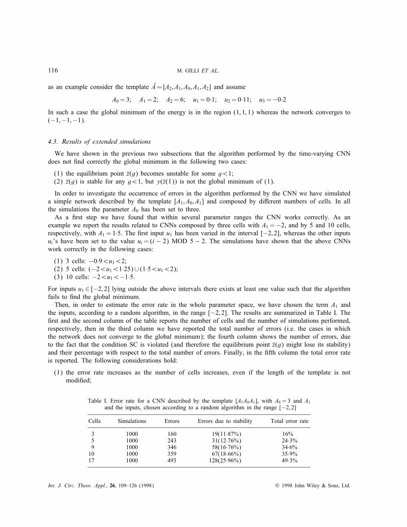
the inputs, according to a random algorithm, in the range [−2; 2]. The results are summarized in Table I. The�rst and the second column of the table reports the number of cells and the number of simulations performed,respectively, then in the third column we have reported the total number of errors (i.e. the cases in whichthe network does not converge to the global minimum); the fourth column shows the number of errors, dueto the fact that the condition SC is violated (and therefore the equilibrium point z(g) might lose its stability)and their percentage with respect to the total number of errors. Finally, in the �fth column the total error rateis reported. The following considerations hold:

(1) the error rate increases as the number of cells increases, even if the length of the template is notmodi�ed;

Table I. Error rate for a CNN described by the template [A1A0A1], with A0 = 3 and A1and the inputs, chosen according to a random algorithm in the range [−2; 2]

Cells Simulations Errors Errors due to stability Total error rate

3 1000 160 19(11·87%) 16%5 1000 243 31(12·76%) 24·3%9 1000 346 58(16·76%) 34·6%10 1000 359 67(18·66%) 35·9%17 1000 493 128(25·96%) 49·3%



(2) the percentage of errors due to the fact that the condition SC is violated increases with the number ofcells.

Note that we have veri�ed that by increasing the number of simulations the error rate does not changesigni�cantly.

5. CONCLUSIONS

We have studied the global optimization properties of a time-varying CNN, whose output function slope isslowly increased from 0 to 1 (i.e. the model introduced in References 1 and 2). We have shown the following:

(1) the only CNN which converges to the global minimum of the quadratic energy function (1) for anyvector u and any entry of the matrix A (with the only constraint that A0¿1), is the network composedby only 2 cells;

(2) if the dimension is higher than 2, even the CNN described by the simplest one-dimensional space-invariant template A= [A1; A0; A1], fails to �nd the global minimum in a subset of the parameter space;the above statement is true both for circular and non-circular connections.

The above considerations imply that, apart from the two-cell CNN, there exist no other classes of CNNswith the ability of �nding the global minimum for any entries of matrix A and of vector u. In fact a CNNdescribed by a generic, even multidimensional template, can be always reduced to the CNN described by thetemplate A= [A1; A0; A1] by simply setting to zero all the other entries.Extensive simulations have shown that for a CNN described by the template [A1; A0; A1], with the parameters

chosen according to a random algorithm, the error rate increases with the number of cells.However, the simulations have also pointed out that within some parameter ranges the time-varying CNN

works correctly.

ACKNOWLEDGEMENT

This research was entirely supported by Consiglio Nazionale delle Ricerche, Rome, Italy, under contributionsno. 9400015.CT07 and no. 96.01762.CT11.

APPENDIX I

This appendix is devoted to the proof of the following proposition.

Proposition 1. A su�cient condition for the stability of the equilibrium point z(g) is that all the co-ordinatesof z(g) which reach a saturation value ±1; for a given g; by increasing g do not come back to the linearpart of the output characteristic.

Proof. For small values of g (i.e. g= ”) the equilibrium point z(g) lies in the central region and its explicitexpression is given by (see (5))

z(g)= (I − gA)−1gu (14)

The stability of z in the central region depends on the sign of the real part of the eigenvalues of the matrixgA− I ; for g= ” such eigenvalues approaches −1 and therefore z is stable.It is easily shown that if for any g∈ [”; gc] the equilibrium z(g) belongs to the central region, then for the

same values of g it is stable. In fact for g= ” the determinant D(g) of the matrix −I+gA is negative; if thereexists a value g2¡gc such that an eigenvalue becomes positive, then D(g2)¿0; since D(g) is a continuousfunction of g, there exists a value g1¡g2¡gc such that D(g1)= 0. But for such a value g= g1, at least one


118 M. GILLI ET AL.

co-ordinate of |z(g)| would tend to ∞. This implies that z(g) leaves the central region for g¡g1¡gc, therebycontradicting the fact that z(g) belongs to the central region for any g∈ [”; gc]. It is concluded that as longas z lies in the central region, it is stable.Suppose now that at g= gc the equilibrium point crosses the border between the central region and a

generic partial saturation region, Rp. In this region, we denote with l and s the set of the non-saturated andof saturated variables, respectively.At g= gc the equilibrium point lies on the border between the central region and region Rp. Therefore its

co-ordinates can be expressed both by (14) (with g= gc) and by the following equation:

zl(gc)= (I − gcAl; l)−1(gcAl; sy s + gcul) (15)

zs(gc)= gc(As; lzl(gc) + As; sy s + us) (16)

where the notations above are de�ned in Section 3.2 (step 4 of the algorithm). The stability of z in the partialsaturation region Rp depends on the sign of the eigenvalues of the matrix −I + gAll ( because all the othereigenvalues equal −1). Since all the eigenvalues of the matrix −I + gcA are negative and the matrix All isobtained from A by deleting the rows and the columns belonging to the saturated set s, it turns out that alsothe eigenvalues of −I + gcAll are negative. Then, by increasing g, as long as the equilibrium point lies inregion Rp, the eigenvalues of −I + gAll remain negative; otherwise the determinant of the matrix −I + gAllwould become zero for some g, thereby implying that z goes out of Rp. If the saturated components of z donot come back to the linear part of the output characteristic, then by increasing g; z will reach the borderof another partial saturation region, whose matrix All can be obtained from the previous one, by deletingsome rows and columns. Therefore the same considerations of above apply and the thesis of Proposition 1is proved.

APPENDIX II

This appendix is devoted to the proof of Theorem 1.

Theorem 1. If the variation of the scalar function g(t) is slow enough; then the global optimization algorithmperformed by the time-varying CNN described by equation (2), with A0¿1; is correct for matrices A∈R2;2;i.e. for networks composed by only two cells.

Proof. If the variation of g is slow enough we have already pointed out in Section 3.1, that the dynamics ofthe time-varying CNN (2) can be studied by considering g as the scalar bifurcation parameter of the dynamicsystem below (with z= gx):

z1 =−z1 + gA0y(z1) + gA1y(z2) + gu1z2 =−z2 + gA1y(z1) + gA0y(z2) + gu2 (17)

where we have denoted by A1 the non-diagonal entries of matrix A (i.e the non-central element of the space-invariant template describing the two-cell CNN).We will prove that by increasing g, the equilibrium point z(g) moves towards the saturation region, where

the quadratic function (1) presents its global minimum, over the hypercube D2.We �rstly prove the following Lemma.

Lemma 1. if A0¿1 then the global minimum of the function (1) occurs in a vertex of the hypercube; i.e.in a saturation region of the network state-space.

Proof. For g=1 the CNN described by equation (5) is completely stable because the matrix A is symmetric(see Reference 9). Since A0¿1 all the stable equilibrium points are located in the saturation regions. Moreover,



it is shown in Reference 9 that the derivative of the energy function (1) with respect to time is negative inthe whole state space, with the exception of a set of measure zero, where it is null. We claim that the globalminimum must occur in a saturation region (i.e. in a vertex of the hypercube). In fact, if this were not thecase the global minimum would occur in an equilibrium point that belongs to a partial saturation region orto the central region where dE(y(x(t))=dt=0. But since such a point is unstable a small perturbation wouldcause a trajectory divergent from the equilibium point, with the property that along it dE(y(x(t))=dt¡0. Thisprevents that the global minimum occurs in an unstable equilibrium point.

Then we will show that the parameter space (A1; u1; u2) can be divided in four subspaces. For each subspacewe show that the equilibrium point z converges towards the vertex of the hypercube (i.e. the saturation regionof the network), which corresponds to the global minimum of the function (1) among the four vertices ofthe hypercube. This is, according to Lemma 1, the global minimum of the function (1) over the wholehypercube D2.We de�ne the following parameter subspaces that cover the whole parameter space and have a null inter-

section:

(1) S1 = S11 ∪ S12– S11 = {(A1; u1; u2): (u1¡−|u2|) ∩ (u2¿A1)}– S12 = {(A1; u1; u2): (u2¿|u1|) ∩ (u1¡−A1)}

(2) S2 = S21 ∪ S22– S21 = {(A1; u1; u2): (u1¿|u2|) ∩ (u2¡−A1)}– S22 = {(A1; u1; u2): (u2¡−|u1|) ∩ (u1¿A1)}

(3) S3 = S31 ∪ S32– S31 = {(A1; u1; u2): (u1¿|u2|) ∩ (u2¿−A1)}– S32 = {(A1; u1; u2): (u2¿|u1|) ∩ (u1¿−A1)}

(4) S4 = S41 ∪ S42– S41 = {(A1; u1; u2): (u1¡−|u2|) ∩ (u2¡A1)}– S42 = {(A1; u1; u2): (u2¡−|u1|) ∩ (u1¡A1)}

The explicit computation of the energy function (1) over the four verteces of the hypercube D2, andLemma 1 permit to state the following:

(1) if the parameters belong to subspace S1 then the global minimum of (1) occurs at y=(−1; 1)′;(2) if the parameters belong to subspace S2 then the global minimum of (1) occurs at y=(1;−1)′;(3) if the parameters belong to subspace S3 then the global minimum of (1) occurs at y=(1; 1)′;(4) if the parameters belong to subspace S4 then the global minimum of (1) occurs at y=(−1;−1)′;We �rstly consider subspace S1, which is composed by the union of S11 and S12 whose intersection is null.

In particular we concentrate on S11 and prove in detail that if the parameters (A1; u1; u2) belong to S11, thenthe equilibrium point z(g) converges towards the saturation region (−1; 1), which is the global minimum ofthe quadratic function (1) over the hypercube D2.For a small g= ”, the system described by equation (17) exhibits only one globally asymptotically stable

equilibrium point, close to the origin and therefore belonging to the central region. By increasing g theevolution of the equilibrium z(g) is described by the following equation:

z(g)=− g(e′1 · u�1

e1 +e′2 · u�2

e2

)(18)


120 M. GILLI ET AL.

where �1, �2, e1, e2, are the eigenvalues and the eigenvectors, respectively, in the central region, i.e.

�1 = g(A0 − A1)− 1�2 = g(A0 + A1)− 1e1 = 1√

2(1;−1)′

e2 = 1√2(1; 1)′

(19)

The following considerations hold:

(1) for a small value of g the two eigenvalues are both negative and close to −1;(2) since A0¿1, by increasing g from ” to 1 at least one eigenvalue �∗ ∈ {�1; �2} becomes positive; since

the two eigenvalues are continuous with respect to g, there exists a value g∗ such that �∗(g∗)= 0;(3) since z(g) is proportional to the inverse of the eigenvalues, before �∗ becomes zero (i.e. for g¡g∗)

the equilibrium z(g) has to reach the border of the central region; moreover as long as z belongs tothe central region, both the eigenvalues are negative and therefore the equilibrium is stable.

From the de�nition of S11 and by use of (19) it is seen that the following inequalities are satis�ed:

e′1 · u =1√2(u1 − u2)¡0

e′2 · u =1√2(u1 + u2)¡0

(20)

Owing to the above inequalities, by use of (18) and of the explicit expression of the two eigenvectors e1and e2 it is easily derived that by increasing g the equilibrium z moves towards the region (−1; X ), i.e. thereexists a values gXX;−1X such that z1(gXX;−1X )= − 1 and |z2(gXX;−1X )|¡1.In region (−1; X ), as in the other partial saturation regions (i.e. where one variable is saturated, whereas the

others work in the linear part of the output characteristic) the two eigenvalues are �1 = gA0− 1 and �2 = − 1.From (17) it is derived that the evolution of z(g) in region (−1; X ) is described by the following equations:

z1(g) =− ggA0 − 1[g(A

20 − A21 + A1u2 − A0u1) + (u1 − A0)]

z2(g) =− ggA0 − 1(u2 − A1)

(21)

The following considerations hold:

(1) At g= gXX;−1X both the eigenvalues of the matrix gA− I are negative; therefore also gXX;−1X A0 − 1 isnegative.

(2) Since in subspace S11; u2¿A1, by increasing g, before that the eigenvalue �1(g) becomes null, theco-ordinate z2(g) tends to saturate to the value 1.

(3) The condition (SC) is satis�ed, i.e. the equilibrium point z(g) cannot come back to the central region.In fact from equation (21) it is seen that the variable z1(g) takes the value −1 for two values of g;the �rst one is gXX;−1X , where as the second one is reported below:

g−1X;XX =−(k2 − A0) +√

((k2 − A0)2 − 4k1)2k1

(22)

wherek1 = A20 − A21 + A1u2 − A0u1 k2 = u1 − A0



Table II. Path followed by the equilibrium point z, for parameters belonging to di�erentsubsets of the parameter space

Parameter subspaces Partial saturation region Saturation region Global minimum

S11 −1; X −1; 1 −1; 1S12 X; 1 −1; 1 −1; 1S21 1; X 1;−1 1;−1S22 X;−1 1;−1 1;−1S31 1; X 1; 1 1; 1S32 X; 1 1; 1 1; 1S41 −1; X −1;−1 −1;−1S42 X;−1 −1;−1 −1;−1

On the other hand from equation (21), we derive that the variable z2(g) reaches the saturation value+1, if the following constraint is satis�ed:

z2(g)¿1→ g¿g−1X;−11 =1

u2 + A0 − A1 (23)

Now in order that the equilibrium point z does not come back to the central region it is su�cient toimpose

g−1X;−11¡g−1X;XX (24)

By substituting expressions (22) and (23) for g−1X;−11 and g−1X;XX , after some algebraic manipulationsthe above inequality (24) reduces to the following one:

(u1 + u2)(u2 − A1)¡0 (25)

which in the parameter subspace S11 is always satis�ed, because u2¿A1 and u1¡− | u2 | . There-fore, the equilibrium z(g) does not come back to the central region, but reaches the saturation re-gion (−11), where the global minimum of the energy function (1) occurs. Since by increasing gthe equilibrium point cannot leave the saturation region, this proves that if the parameters lie inthe subspace S11, then the equilibrium point z(g) converges to the saturation region (−1; 1), i.e. tothe vertex where, according to Lemma 1, the energy function (1) presents its global minimum over thehypercube D2.

As far as the other parameter subspaces are concerned, it is possible to prove the correctness of thealgorithm performed by the CNN by following exactly the same procedure developed above. The results aresummarized in Table II, where for each subspace we have reported the partial saturation region crossed by zand the saturation region, which is the �nal destination of z. We have veri�ed that in all cases the condition(SC) is satis�ed. We remark that the same proof can be carried out also for parameters lying on the boundaryamong two or more parameter subspaces. In such cases there are more than one vertices where the energyfunction takes the global minimum; moreover the equilibrium point z may directly migrate from the centralregion to a saturation region. Since such situations occur for set of parameters of measure zero we do notreport the detailed proof.

APPENDIX III

This appendix is devoted the proof of the following theorem:


122 M. GILLI ET AL.

Theorem 2. If the variation of the scalar function g(t) is slow enough; then the global optimization algorithmperformed by the time-varying CNN described by equation (2) is correct for matrices A (i.e. for networks)with the property that there exists a real number g∗ such that the non-linear system

z=− z + g∗Ay(z) + g∗u (26)

exhibits one and only one stable equilibrium point; z(g∗); and such an equilibrium belongs to a saturationregion (i:e: ∀i |y(zi(g∗)) |¿1).

Proof. For a generic g 6=1 the energy function of the dynamical system described by equation (5) can beeasily obtained by replacing in (1) the matrix A with gA and the input u with gu:

E(y; g)=− 12y

′(gA− I)y − y′gu (27)

By assumption, for g= g∗ there exists only one stable equilibrium point, z(g∗), that represents also theglobal minimum of the energy (27) (see the proof of Lemma 1, and replace the energy (1) with (27)).It is easily proved that by increasing g the point z(g) cannot leave the saturation region and therefore it is

always stable for any g¿g∗. In fact in the saturation region, the evolution of z is described by the followingequation:

z(g)= g(Ay(z(g)) + u) (28)

It is readily veri�ed that, since the output y is constant in the saturation regions and g is positive if z belongsto a saturation region at g= g∗, it remains in the same region for any g¿g∗.Then we prove that the equilibrium point z, that is the global minimum of the energy (27) at g= g∗,

remains the global minimum for any g¿g∗. In order to do that we compute the derivative, with respect to gof the energy function (27). After some algebraic manipulations we obtain

dE(y; g)dg

=1g(E(y; g)− 0:5y′y) (29)

The term y′y takes the minimum values in the saturation regions, where for an n-cell CNN, y′y= n.Moreover, at g= g∗; E(y(z); g∗) is the global minimum of E(y; g∗); (y∈Dn). Therefore, according to (29)at g= g∗ the derivative of E(y(z); g) with respect to g is less than the derivative in any other point of thestate space. Owing to the structure of the di�erential equation (29), to the fact that g¿0 and that z does notleave the saturation region, this implies that E(y(z); g) remains the global minimum for any g¿g∗.

APPENDIX IV


Theorem 3. If the parameters of the circular CNN; described by matrix (12) satisfy the following constraints:

1. u2 = u3;2. u1 + 2 | u2 |¡0;3. A1¿0;4. A1¡u2;5. A1(u2 − u1 − 2A1) + u2(u1 + u2)¿0;

then the equilibrium point z(g) becomes unstable and this prevents from a correct behaviour of the network.



Proof. Firstly we show that conditions 1–3 guarantee that by increasing g the equilibrium z(g) moves fromthe central region towards the partial saturation region where y(z1)=− 1 (i.e. region (−1; X; X )). By use ofcondition 1, the explicit computation of the evolution of z(g) in the central region yields

z(g)= (I − gA)−1gu= gD(g)

(1− gA0 − 2gA1) u1 + gA1 (u1 + 2u2)(1− gA0 − 2gA1) u2 + gA1 (u1 + 2u2)(1− gA0 − 2gA1) u2 + gA1 (u1 + 2u2)

(30)

where

D(g)= (1− gA0 + gA1)(1− gA0 − 2gA1) (31)

For a small g= � the term D(g) is positive; by resorting to the proof of Proposition 1, it is easily shownthat as long as z lies in the central region, D(g) remains positive.Condition 1 ensures that in the central region z2(g)= z3(g). Since D(g) is positive, by using conditions 2

and 3, from expression (30) we have

| z2(g) | = | (1− gA0 − 2gA1) u2 + gA1 (u1 + 2u2) | (32)

6 | (1− gA0 − 2gA1) u2 | + | gA1 (u1 + 2u2) | (33)

= (1− gA0 − 2gA1) | u2 | + gA1 | (u1 + 2u2) | (34)

6 (1− gA0 − 2gA1) | u1 | + gA1 | (u1 + 2u2) | (35)

= | (1− gA0 − 2gA1) u1 + gA1 (u1 + 2u2) | (36)

= | z1(g) | = − z1(g) (37)

This proves that by increasing g, the equilibrium z(g) moves towards the partial saturation region wherey(z1)=−1, i.e. there exists a g, such that for any �6g¡g; z(g) belongs to the central region and y(z1(g))=−1.Then we prove that conditions 1–5 together imply that by further increasing g the equilibrium z(g) moves

back to the central region for a value of g¿1=(A0 + 2A1), i.e. such that the central region is unstable.According to step 4 of the algorithm (formulas 7 and 8), for g¿g the evolution in the partial saturation

region (−1; X; X ) is described by the following equations:

z1(g)=[2A1(u2 − A1)− (u1 − A0)(A0 + A1)]g2 + (u1 − A0)g

1− g(A0 + A1) (38)

z2(g)= z3(g)=(u2 − A1)g

1− g(A0 + A1) (39)

For g= g the equilibrium z(g) is stable (i.e. all the eigenvalues of matrix A are negative); therefore alsothe eigenvalues of the matrix obtained by deleting from A the �rst column and the �rst row are negative(in particular g(A0 + A1)− 1¡0).This implies that if condition 4 is satis�ed then the variable z2(g)= z3(g) is positive for g¿g.Now, it is seen from equation (38) that z1(g) takes the value −1 for two values of g; the �rst one is g= g,

whereas the second one turns out to be

g∗= c1 + c0 +√((c1 + c0)2 − 4c2)2c2

(40)


124 M. GILLI ET AL.

where

c0 = A0 + A1

c1 = A0 − u1c2 = 2A1(u2 − A1)− (A0 + A1)(u1 − A0) (41)

On the other hand from equation (39), we derive that the variable z2(g) does not reach the saturation value,if the following constraint is satis�ed:

z2(g)¡1→ g¡g∗∗=1=c3 (42)

where

c3 = 1=(u2 + A0) (43)

Now, in order that the equilibrium point z comes back to the central region (i.e. the variable z1 crossesback the value −1 whereas the variable z2 = z3 does not leave the linear part of the output characteristic), itis su�cient to impose

g∗¡g∗∗ (44)

Since conditions 2–4 imply that c2¿0, the above inequality reduces to

c3(c1 + c0 +√((c1 + c0)2 − 4c − 2))¡2c2 (45)

and after some algebraic manipulation it turns out that if condition 5 is veri�ed then (45) holds. Henceconditions 1–5 imply that the equilibrium z(g) for g= g∗ comes back to the central region, thereby violatingthe condition (SC). Moreover, it is easily veri�ed that under conditions 1–5, g∗¿1=(A0 +2A1). Therefore forg= g∗ the equilibrium z(g) looses its stability.

APPENDIX V


Theorem 4. If the parameters of the CNN; described by matrix (13) satisfy the following constraints:

1. u2 =− u3¡0;2. A0¿1;3. A1¿M¿0; where M is a suitable large constant;4. 0¡u1¡�; where � is a suitable small constant

then the time-varying CNN converges towards the saturation region (−1;−1;−1) whereas the global mini-mum of the energy (1) occurs in region (1; 1; 1).

Proof. Since A0¿1; at g=1, all the stable equilibria of the CNN described by equation (5) lie in a saturationregion. Therefore; according to the proof of Lemma 1 (which is simple to extend from dimension 2 to 3) theglobal minimum of the function (1) occurs in a vertex of the hypercube D3.The explicit evaluation of function (1) over the 8 vertices of the hypercube D3, shows that if M¿ | u1 | +

| u2 | + | u3 | (condition 3) and u1 + u2 + u3¿0 (conditions 1 and 4), the global minimum occurs in region(1; 1; 1).



The evolution of the equilibrium point z(g) in the central region is described by the following equations:

z(g)=g

D(g)

(1− gA0)2 − (gA1)2 (1− gA0)gA1 (gA1)2

(1− gA0)gA1 (1− gA0)2 (1− gA0)gA1(gA1)2 (1− gA0)gA1 (1− gA0)2 − (gA1)2

u1

u2

u3

(46)

where

D(g)= (1− gA0)[(1− gA0)2 − 2(gA1)2] (47)

If the term u1 is small enough with respect to | u2 | and | u3 | (condition 4) then in equation (46) the termsmultiplying u1 can be neglected. We obtain (by use of condition 1):

z1(g) ≈ gD(g)

[(1− gA0)gA1 − (gA1)2]u2

z2(g) ≈ gD(g)

[(1− gA0)2 − (1− gA0)gA1]u2 (48)

z3(g) ≈ gD(g)

[(1− gA0)gA1 − (1− gA0)2 + (gA1)2]u2We remark that as long as the equilibrium z lies in the central region, the determinant of matrix I − gA

(i.e. D(g)) remains positive (see Proposition 1). Owing to the fact that D(g)¿0 and A1¿0 (condition 3),the following inequality holds:

1− gA0 − gA1¿0 (49)

From equations (48), after simple algebraic manipulations it is easily seen that if (49) is veri�ed, then thetwo inequalities below are satis�ed:

| z1(g) |¡−z2(g)| z3(g) |¡−z2(g) (50)

thereby implying that, by increasing g the variable z2(g) saturates to the value −1, i.e. a transition betweenthe central region and the partial saturation region (X;−1; X ) occurs.In such a region the system exhibits two eigenvalues equal to −1 + gA0 (that are negative because the

condition (SC) is satis�ed). The evolution of the equilibrium point z(g) in region (X;−1; X ) is given by thefollowing equations:

z1(g) =g(u1 − A1)1− gA0

z2(g) =−gA0 + g2A11− gA0 (u1 + u3 − 2A1) + gu2

z3(g) =g(u3 − A1)1− gA0

(51)

From the above equations it is veri�ed if M is large enough (condition 3) then the variable z2(g) doesnot come back to the linear part of the output characteristic (i.e. condition (SC) continues to be satis�ed)and that the variable z1(g) saturates to the value −1 (because due to condition 4, | u1 | is less than | u3 | ).Therefore, a transition from region (X;−1; X ) to region (−1;−1; X ) occurs. Then by computing the evolution


126 M. GILLI ET AL.

of the equilibrium z in region (−1;−1; X ) it is readily veri�ed that eventually also the variable z3 convergesto −1, i.e. the CNN converges to an equilibrium point lying in region (−1;−1;−1), which does not containthe global minimum.

REFERENCES

1. B. J. Sheu, R. C. Chang, T. H. Wu and S. H. Bang, ‘VLSI-compatible cellular neural networks with optimal solution capability foroptimization’, Proc. 1995 Int. Symp. Circuits Systems, Seattle, May 1995, pp. 1165–1168.

2. S. H. Bang, B. J. Sheu and E. Y. Chou, ‘A Hardware annealing method for optimal solutions on cellular neural networks’, IEEETrans. Circuits Systems. Part II, 43, 409–421 (June 1996).

3. P. M. Pardalos and J. B. Rosen, ‘Constrained global optimization: algorithms and applications’, Lectures on Computer Science,Springer, Berlin, 1987.

4. F. Barahona, ‘A solvable case of quadratic 0–1 programming’, Discrete Appl. Math. 13, 23–26 (1986).5. M. R. Garey and D. S. Johnson, Computers and Intractability: a Guide to the Theory of NP-completeness, Freeman, San Francisco,1979.

6. P. L. Hammer, P. Hansen, and B. Simeone, ‘Roof duality, complementation and persistency in quadratic 0–1 optimization’, Math.Programming 28, 121–155 (1984).

7. A. Cichocki and R. Unbehauen, Neural Networks for Optimization and Signal Processing, Wiley, New York, 1993.8. E. Aarts and J. Korst, Simulated Annealing and Boltzmann machines. A Stochastic Approach to Combinatorial Optimization andNeural Computing, Wiley, New York, 1989.

9. L. O. Chua and L. Yang, ‘Cellular neural networks: theory’, IEEE Trans. Circuits Systems, 35, 1257–1272 (1988).10. L. O. Chua and T. Roska, ‘The CNN paradigm’, IEEE Trans. Circuits Systems. Part I, 40, 147–156 (1993).


analysis of time-varying cellular neural networks for quadratic global optimization

Documents