analysis of suspended bridges for isolated...
TRANSCRIPT

Avdelningen för Konstruktionsteknik
Lunds Tekniska Högskola
Box 118
221 00 LUND
Division of Structural Engineering
Faculty of Engineering, LTH
P.O. Box 118
S-221 00 LUND
Sweden
Analysis of suspended bridges for isolated communities
- With emphasis on wind stability
Analys av lätta hängbroar för isolerade samhällen
- Med fokus på vindstabilitet
Viktor Hermansson & Jonas Holma
2015

Rapport TVBK-5243
ISSN 0349-4969
ISRN: LUTVDG/TVBK-15/5243+88p
Examensarbete
Examinator: Professor Roberto Crocetti, LTH
Handledare: Anders Klasson, LTH
Handledare: Ivar Björnsson, LTH
Handledare: Karl Lundstedt, SKANSKA
Handledare: Gustav Svensson, SKANSKA
Juni 2015
Abstract
Light suspended bridges are often used to connect villages or trail systems in geographical areas
with lacking infrastructure and demanding topology. Different international non-profit
organizations in collaboration with local promoters are building these bridges with the purpose
of connecting isolated communities with health care and education.
The design and construction of these bridges has by and large relied on engineering judgment
and design conservatism coupled with past experiences of similar construction projects. An
interest to engage in the designing of similar bridges has been shown from staff at the Division
of Structural Engineering at the Faculty of Engineering of Lund University. This master thesis
aims therefore to provide more sophisticated models of suspended bridges as material for future
work.
Suspended bridges are suitable to use for long spans, both due to low construction cost and to
efficient material usage. They can also most often be built without advanced tools or machinery.
The bridges studied in this thesis are intended for pedestrians and animals which result in a very
slim design.
Recommendations mainly from the development organization Helvetas will be compared to the
Eurocode to investigate if these creates overly conservative designs. These comparisons will be
made with both hand calculations, the finite element software Brigade/Plus and data from
existing bridges.
Vibrations and sways due to wind can be a major problem for light suspended bridges. Due to
their small dead load in combination with a low lateral stiffness, the sways and vibrations can
be very large in comparison with more common pedestrian bridges. This could lead to
temporary inoperability or in worst case structural failure. With the models made in
Brigade/Plus, wind effects can be analyzed and suitable measures or restrictions can be
proposed.
Key words: Suspended bridge, wind loads, dynamic response, vibrations, cables, FE-analysis,
modal superposition.


Sammanfattning
Lätta hängbroar används ofta för att sammankoppla samhällen i områden med bristande
infrastruktur och krävande topologi. Dessa broar byggs genom samarbete mellan internationella
hjälporganisationer och lokala initiativtagare med syftet att tillgängliggöra sjukvård och
utbildning.
Designen på de broar som byggs bygger ofta på empiriska erfarenheter. Intresse för att engagera
sig i dimensionering av liknande broar har visats från personal på Avdelningen för
Konstruktionsteknik vid Lunds Tekniska Högskola. Denna uppsats syftar därför på att skapa en
mer precis dimensionering av dessa broar som underlag för framtida arbete.
Lätta hängbroar är en mycket materialeffektiv konstruktion som kan överbrygga långa spann
till ett relativt lågt pris. De kan dessutom oftast byggas utan avancerade verktyg eller maskiner.
De broar som studeras är alla avsedda för gångtrafik från människor och djur vilket medför en
slank design.
Rekommendationer från främst organisationen Helvetas jämförs med Eurocode för att utreda
om dessa skapar onödigt robusta konstruktioner. Dessa jämförelser sker med både
handberäkningar, finita element-programmet Brigade/Plus samt data från existerande broar.
Vibrationer och svängningar orsakade av vind kan innebära ett stort problem för lätta
hängbroar. På grund av deras låga egentyngd samt deras låga styvhet i transversell riktning kan
dessa svängningar bli mycket stora i jämförelse med mer vanliga gångbrotyper. Detta kan leda
till att bron blir tillfälligt obrukbar eller i värsta fall blåser sönder. Med de modeller som byggs
upp i Brigade/Plus kommer vindeffekter att kunna analyseras och lämpliga åtgärder eller
begränsningar föreslås.
Nyckelord: Hängbro, vindlaster, dynamisk respons, vibrationer, kablar, FE-analys, modal
superpositionering


“What would be the best bridge? Well, the one
which could be reduced to a thread, a line,
without anything left over; which fulfilled
strictly its function of uniting two separated
distances.”
Pablo Picasso
Preface
This master thesis is the final phase of our five year Master Program in Civil Engineering at the
Faculty of Engineering, LTH, at Lund University. As always in the start of a project, this thesis
had a very wide objective, which during the last months has made us humble to how much we
still have to learn. However, this has been the most intensive and educational time during our
time at the university.
The subject of this thesis was proposed by the Division of Structural Engineering and the thesis
has been carried out at Skanska AB in Malmö.
There are many people we would like to thank, especially our examiner Professor Roberto
Crocetti and our supervisors Anders Klasson and Ivar Björnsson at the Division of Structural
Engineering for all your ideas and support, and Karl Lundstedt and Gustav Svensson at Skanska
Malmö for all the good advice and for letting us be a part of your team for half a year.
We would also like to thank Helvetas and Bridges to Prosperity for providing us with helpful
material, and Scanscot Technology for their Brigade/Plus support.
Finally we would like to thank our families and friends for all their support during these years,
and last, but by no means least, all our classmates in whose company these years have been
fantastic.
Lund June 2015
Viktor Hermansson & Jonas Holma


Innehållsförteckning
1 Introduction ..................................................................................................................1
1.1 Background ..............................................................................................................1
1.2 Aim ..........................................................................................................................3
1.3 Limitations ...............................................................................................................3
1.4 Outline .....................................................................................................................4
2 Background theory .......................................................................................................5
2.1 History of suspended and suspension bridges ...........................................................5
2.2 Description of a typical suspended bridge .................................................................5
2.3 Suspended bridges in aid projects .............................................................................6
2.4 Helvetas and Bridges to Prosperity ...........................................................................6
2.5 Cables ......................................................................................................................7
2.5.1 Types of cables..................................................................................................7
2.5.2 Cables as load bearing element ..........................................................................9
2.6 Statics..................................................................................................................... 11
2.7 Dynamics of cables ................................................................................................ 13
2.7.1 Dynamic behavior of the single cable .............................................................. 13
2.8 Wind effects ........................................................................................................... 18
2.8.1 Buffeting ......................................................................................................... 18
2.8.2 Flutter ............................................................................................................. 18
2.8.3 Vortex shedding .............................................................................................. 18
2.8.4 Galloping ........................................................................................................ 18
2.9 Comfort criteria ...................................................................................................... 19
2.9.1 Eurocode ......................................................................................................... 20
2.9.2 Sétra ................................................................................................................ 20
2.9.3 JRC- and ECCS-report .................................................................................... 20
2.9.4 ISO 10137 ....................................................................................................... 21
2.9.5 Nakamura ........................................................................................................ 22
2.9.6 Summary and suggestions ............................................................................... 23
2.10 Loads .................................................................................................................. 24
2.10.1 Wind loads on bridges ..................................................................................... 24
2.10.2 Static wind loads ............................................................................................. 24
2.10.3 Vertical loads .................................................................................................. 26
2.10.4 Live load ......................................................................................................... 26
2.10.5 The vertical effects from wind load ................................................................. 28

2.10.6 Load combinations .......................................................................................... 28
2.11 Fatigue ................................................................................................................ 29
2.12 Brigade/Plus ....................................................................................................... 29
2.12.1 Equation of motion SDOF ............................................................................... 29
2.12.2 Rayleigh Damping........................................................................................... 30
2.12.3 Newton-Raphson ............................................................................................. 30
2.12.4 Eigenvalue ...................................................................................................... 30
2.12.5 Modal dynamics .............................................................................................. 31
2.12.6 Implicit dynamics ............................................................................................ 31
3 Reference bridge ......................................................................................................... 33
4 Analysis of the single cable ......................................................................................... 35
4.1 Evaluation of sag .................................................................................................... 35
4.2 Modelling of a single cable in Brigade/Plus ............................................................ 40
4.3 Discussion .............................................................................................................. 41
5 Static analysis of the suspended bridge ...................................................................... 43
5.1 Hand calculations ................................................................................................... 43
5.2 Modelling ............................................................................................................... 43
5.3 Influence lines ........................................................................................................ 43
5.4 Displacements ........................................................................................................ 47
5.5 Stress distribution ................................................................................................... 49
5.6 Cable diameter and span ......................................................................................... 51
5.7 Discussion .............................................................................................................. 54
6 Dynamic Analysis........................................................................................................ 57
6.1 Modal superpositioning .......................................................................................... 57
6.1.1 Natural Frequencies ......................................................................................... 57
6.1.2 Excitation / Impulse......................................................................................... 59
6.1.3 Damping ......................................................................................................... 60
6.2 Modal analysis ....................................................................................................... 60
6.2.1 Displacements ................................................................................................. 60
6.2.2 Accelerations................................................................................................... 62
6.3 Implicit dynamic step ............................................................................................. 64
6.4 Discussion .............................................................................................................. 65
7 Conclusions ................................................................................................................. 67

7.1 Further investigations ............................................................................................. 68
8 References ................................................................................................................... 69
9 Annex .......................................................................................................................... 71
9.1 Design guide .......................................................................................................... 71
9.2 Natural frequencies and appurtenant modes ............................................................ 82


1.1 Background
1
1 Introduction
1.1 Background Cable supported bridges are widely used because of their ability to overcome large spans. The
term cable supported bridges includes many different types of bridges, for example suspended-
, suspension- and cable stayed bridges. This thesis will focus on the designing and construction
of suspended bridges.
Figure 1.1 A suspended bridge (With permission from Bridges to Prosperity)
The suspended bridge contains load carrying cables for the walkway and also often for the
handrails. Because of its natural shape the main use is as a pedestrian bridge. The reason for the
widely use of suspended bridges in aid projects around the world is that the structure is
relatively simple and have shown to be convenient for construction in rural areas since it can
cross large span in combination with being material efficient and therefore quite cheap. A
suspended bridge can most often be built without the use of heavy machinery and it requires
very little maintenance.
Suspended bridges has a typical span smaller than 200 meters, but spans up to 350 meters exist,
for example the 337 meter long Arroyo Cangrejillo Pipeline Bridge in Argentine (OPAC
Consulting Engineers, 2015) and the 344 meter long Kusma-Gyadi Bridge in Nepal (Ekantipur,
2015). Longer spans are usually pure suspension bridges but can also be a combination, i.e. a
suspension bridge with very short pylons, for example the 406 meter long Highline179 in
Ruette, Austria. Almost all bridges with spans of this magnitude are stabilized in their lateral
direction with so-called windguys to prevent wind induced movements. A suspended bridge
fitted with windguys can be seen in Figure 1.2.
1.1 Background
2
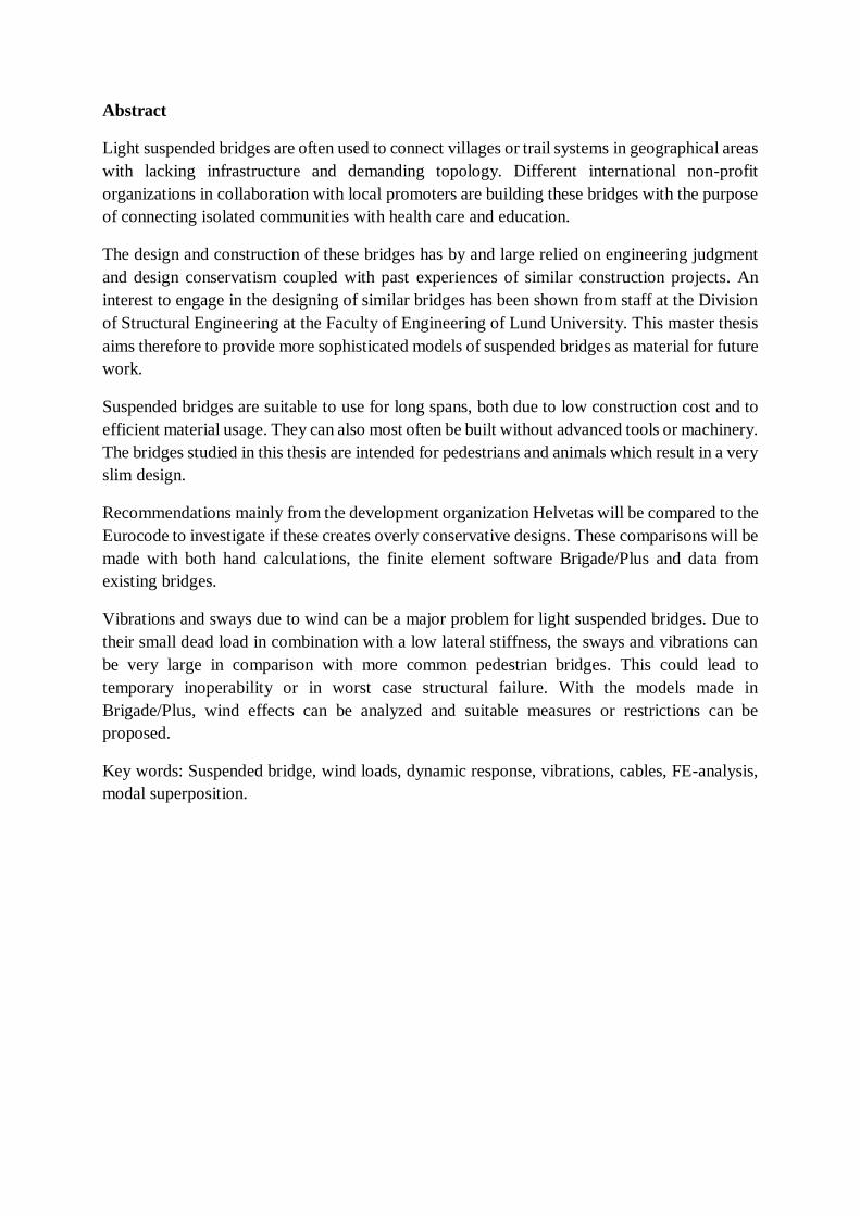
Suspended bridges can also be uses as road bridges, so-called stress ribbon bridges, but in these
cases the deck is made much stiffer and the suspended cables or ribbons are often pre-stressed.
Figure 1.2 A suspended bridge with visible windguy arrangement below (With permission from
Bridges to Prosperity)
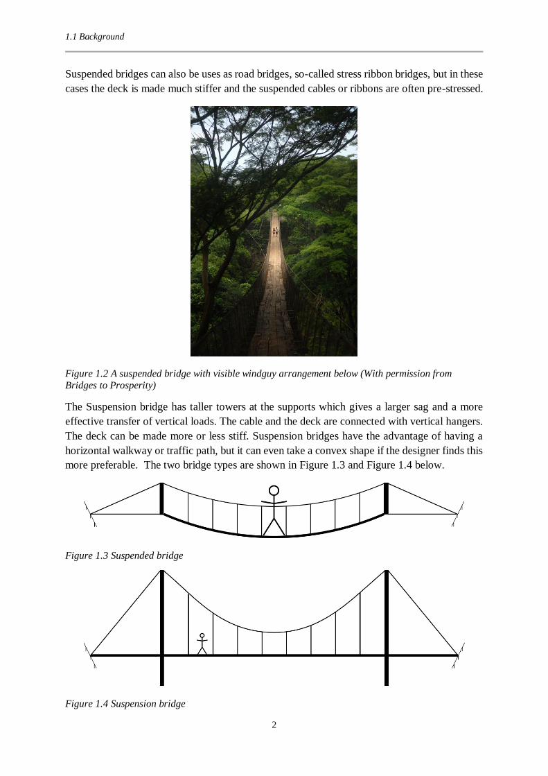
The Suspension bridge has taller towers at the supports which gives a larger sag and a more
effective transfer of vertical loads. The cable and the deck are connected with vertical hangers.
The deck can be made more or less stiff. Suspension bridges have the advantage of having a
horizontal walkway or traffic path, but it can even take a convex shape if the designer finds this
more preferable. The two bridge types are shown in Figure 1.3 and Figure 1.4 below.
Figure 1.3 Suspended bridge
Figure 1.4 Suspension bridge

1.2 Aim
3
1.2 Aim The general aim of this thesis is to highlight suspended bridges and make their design and
structural behavior more understandable for both the general reader of this thesis and,
especially, for future designers of these type of bridges.
The differences between designing according to Helvetas or Eurocode will be investigated since
this can result in a different design criteria and therefore lead to more material efficient and
cheaper bridges.
An investigation of the wind stability of light suspended bridges will be made. The aim of this
investigation is to formulate design criteria for windguys, i.e. when and why they should be
used?
Hand in hand with the wind stability goes the dynamic behavior of suspended bridges. A study
of the natural frequencies and appurtenant modes and how they are affected by the sag and the
span of the bridge will be done.
Another aim of this thesis is to create a design guide in Excel which can be used to design
suspended bridges according to both Helvetas and Eurocode. This guide will make a fast and
accurate design of the bridge main cables possible. A careful comparison between the results
from the design guide and result from finite element models will be done to validate both
methods.
1.3 Limitations It’s only the bridge structure, i.e. the structure between the saddles at the two abutments that
will be analyzed and discussed in this thesis. Everything else, for example design of abutments,
slope stability and technical survey etc, will be left for further investigations. The focus of this
thesis is on the main bearing elements which leads to that no connectors will be investigated.
The type of wind stabilization system used is windguys that are symmetrically designed around
the midpoint of the bridge. Other types of stabilization systems (which obviously exists) will
not be investigated thoroughly.
Vertical dynamic response due to pedestrian traffic will also be out of scope for this thesis.

1.4 Outline
4
1.4 Outline This thesis is divided into 9 different chapters.
Chapter 1 contains an introduction to suspended bridges and a short presentation of the thesis.
Chapter 2 contains background theory of all the forthcoming chapters. Statics and dynamics of
the singe cable, loads and an introduction to the finite element software Brigade/Plus.
Chapter 3 contains a description of the reference bridge.
Chapter 4 contains both static and dynamic analyses of the single cable.
Chapter 5 contains a static analysis of suspended bridges. This includes hand calculations
compared to finite element models, stress distribution between cables, displacements and the
connection between span and cable diameters.
Chapter 6 contains a dynamic analysis of suspended bridges. This includes displacements and
accelerations due to a wind impulse and the determination of natural frequencies.
Chapter 7 contains the conclusions from this thesis.
Chapter 8 contains all the references.
Chapter 9, the annex, contains a design guide and pictures of natural frequency modes.

2.1 History of suspended and suspension bridges
5
2 Background theory
2.1 History of suspended and suspension bridges The model of suspending a rope as main load carrying element has been used for a very long
time. The Incas connected its 39 000 km long networks of roads with suspended bridges made
of ropes (BBC, 2015). An example of such a bridge can be seen in Figure 2.1.
Figure 2.1 A replica of a traditional Inca rope bridge (Dylan Thuras; Atlas Obscura, 2015)
However, the first cable supported structure with drawn iron wires was built in 1823 in Geneva
(Gimsing, 1997). The main types used today are cable-stayed bridges with typical spans up to
1100 meters and suspension bridges with typical spans between 1000 and 2000 meters. For
example the current world record holder for suspended bridges is the Akashi Kaikyō Bridge in
Japan with a main span of 1991 meter. Bridges with longer spans are planned, for example the
Messina strait bridge, and if this bridge ever to be built, its main span will have a length of 3.3
kilometers (COWI, 2015).
2.2 Description of a typical suspended bridge As mentioned in the introduction, the span of the suspended bridges this thesis concerns seldom
exceeds 200 meters. For these bridges the design are often very similar. The two main
foundations are placed on each side of the span and the elevation of them can be either the same
(level bridge) or it can differ (inclined bridge). These main foundations are usually designed as
gravity foundations even if anchorage rods may be used if the space for gravity foundations is
limited. The cables can be attached either adjustable or nonadjustable to the main foundations.
Both the handrail and the lower cables acts as load-bearing elements and they are connected
with hanger rods throughout the bridge. The hanger rods are connected at top to the handrail

2.3 Suspended bridges in aid projects
6
cables and at the bottom to the cross-beams. The cross-beams are bolted to the main cables and
supports the walkway deck. If there is need for wind stabilization, windguys can be added to
the structure. A visualization of the bridge described above can be seen in Figure 2.2 below.
Figure 2.2 A typical suspended bridge
2.3 Suspended bridges in aid projects As described in the introduction suspended bridges are widely used in aid projects around the
world. Communities, that for several months every year are isolated due to impassible rivers,
can with a suspended bridge be provided with a safe route to education, health care and
economic possibilities. The construction of a suspended bridge requires a large community
participation. Community participation during construction includes transport of materials,
collection of locally available materials such as sand, stones and wood and site clearing and
excavation. Since the community will be both the owner and user of the bridge, it will also be
responsible for the long time bridge maintenance and repair
2.4 Helvetas and Bridges to Prosperity Helvetas and Bridges to prosperity are two organizations that designs and builds bridges to
connect isolated communities. Both organizations aims to provide better and safer access to
health care, education and economic opportunities for these communities.
Helvetas Swiss Intercooperation is an aid organization that works in more than 30 countries
(Helvetas, 2015). Since 1972, Helvetas has been involved in trail bridge building in Nepal, and
later on in other countries as well. This work has, in collaboration with other organizations,
ended up in the Short Span Trail Bridge Standard (SSTBS) and the Long Span Trail Bridge
Standard (LSTBS). These two manuals gives guidance for the construction of suspended and
suspension bridges. Both the Short Span Trail Bridge Standard and especially the Long Span
Trail Bridge Standard will be used in this thesis.
Bridges to Prosperity is an American aid organization with focus on bridge building in rural
and isolated areas. Bridges to Prosperity was founded in 2001 and they work mostly in Central
America, South America and Africa. The manual from Bridges to Prosperity are based on the
manuals from Helvetas, with some modifications.

2.5 Cables
7
2.5 Cables
2.5.1 Types of cables Parallel wire cables
Parallel wire cables, as seen in Figure 2.3, are the most widely used
cables in suspension bridges. They consist of a number of wires,
laid parallel and straight throughout the whole length of the cable.
These cables are constructed by in situ spinning or by assembling
a number of preformed parallel wire strands. The void ratio of
parallel wire cables after compaction is generally 18-22 % (Ryall,
Parke, & Harding, 2000). The stiffness of a parallel wire cable is
around E=200 MPa (LTH, Structural Engineering, 2014)
Spiral cables
Spiral cables, as seen in Figure 2.4, consist of a straight center core
wire with multiple layers of round steel twisted around it. Each
layer of wires is twisted in the opposite direction to the preceding
layer. The twist of the wires result in a 15-25 % decreased stiffness
and the cable strength is reduced to around 90 % of the sum of the
breaking strength of the individual wires (Ryall, Parke, & Harding,
2000). The stiffness of a spiral cable is around E=150 MPa (LTH,
Structural Engineering, 2014).
Locked coil cables
Locked coil cables, as seen in Figure 2.5, are very similar to spiral
cables. They consist of, just like spiral cables, a straight center core
wire with multiple layers of round steel twisted around it. They
differ in that the final layers of wire consist of Z-shaped wires.
These wires lock into each other and create a smooth exterior
surface. The Z-shaped wires also minimize the void space in the
cross-sectional area. The compact outer layers of the cable make
protective wrapping unnecessary, but they make inspection and
maintenance of the inner strands difficult (Ryall, Parke, & Harding,
2000). The stiffness of locked coil cables is around E=160 MPa
(LTH, Structural Engineering, 2014).
Wire rope / Strand rope
Wire rope, as seen in Figure 2.6, usually consists of 6 spiral cables
twisted around a core strand, but the number can vary a lot. The core
could be made of either steel or synthetic material. Wire ropes are very
flexible which makes them suitable for cranes, ski lifts etc. The
flexibility depends on the choice of material of the core. A ropewith a
synthetic core is more flexible than a rope with a steel core but it’s
Figure 2.4 Spiral cable
Figure 2.5 Locked
coil cable
Figure 2.6 Wire rope /
Strand rope
Figure 2.3 Parallel wire
cable

2.5 Cables
8
more sensitive to crushing than the steel core rope. Wire rope is not usually used in bigger
suspension bridges since the other types of cables mentioned above are more suitable for this
purpose (LTH, Structural Engineering, 2014). However, in this dissertation wire rope will be
used as main load carrying element since it’s the most common solution for suspended bridges
in rural and remote areas. Wire rope is a mass fabricated standard product which makes it more
affordable and more available in areas where this type of bridges are built. The stiffness of wire
rope varies a lot, but the wire rope that will be used in this dissertation has a Young’s modulus
of around E=110 GPa (Helvetas, 2004).
Wire rope is elastic and it will stretch or elongate when it’s subjected to a tensile force. This
stretch can be divided into three different phases which depends on the magnitude of the force
and the lifetime-situation of the cable.
Phase 1 – Constructional extension
When a wire rope is subjected to a load for the first time, the helically-laid wires will act in a
constricting manner which will lead to a compression of the core and a more tight contact of all
the rope elements. The constructional extension depends on the core material, the wire
construction and the steel quality. Ropes with fiber core extends more than ropes with steel
core. This is because the steel cannot compress as much as the synthetic core. Because of these
different factors it’s hard to set at definite value of the constructional extension. Approximate
values is 0.25 % - 0.5 % for a rope with steel core and 0.75 % - 1 % for a rope with synthetic
core (Hanes Supply, 2015).
Phase 2 – Elastic extension
Following phase 1, an elastic extension resulting mostly from recoverable deformation on the
metal will occur. The manner of this extension complies approximately with Hooke’s law which
makes it possible to quite easy calculate the elastic extension. It’s important to note that the
Young’s modulus of a wire rope is only an approximation because of the non-homogenous
cross section. This “apparent” Young’s modulus can be obtained from the manufacturer or by
making a modulus test on an actual wire rope sample.
Phase 3 – Permanent extension
Just as any other metallic structural member, wire rope has a yield point. If the tensile stress in
the wire rope exceeds the yield stress, permanent extension will occur.
Beyond these three types of extensions, both thermal extension, extension due to rotation and
extension due to wear can appear, but they won’t be taken into consideration in this thesis.

2.5 Cables
9
2.5.2 Cables as load bearing element In a comparison between using a single cable or beam as load-carrying elements for transversal
load, the two show different behavior. Due to its low bending stiffness, a cable works in almost
pure tension whilst a beam carries load by combining compression and tension in its cross
section. For simplicity it’s assumed that the cable has no bending stiffness and can therefore
only transfer load by tension. For the cable it means that the geometrical configuration is of
absolute importance, i.e. the sag. A straight cable is unable to carry any transversal load. With
a cable there will also be a horizontal reaction at the supports in Figure 2.7 which often is larger
than the vertical reaction. The beam will only be subjected to a vertical reaction at the supports.
Figure 2.7 Support reactions for a cable and a beam
The advantage in using cables compared to beams is material efficiency. This is because the
cables transfer load in the most efficient way, pure tension. Gimsing (Gimsing, 1997) illustrated
this by comparing a cable with a sag of 3 meters and a beam for the same load case, see Figure
2.8.
Figure 2.8 A cable and a beam designed for a uniform load, 27 kN/m, over a 30 meter span
For this given load case and span the amount of structural material used with a cable as load-
carrying elements is substantial less than with a beam, which can be seen in Figure 2.8 above.
A cable is showing more geometrical change due to different loading than a beam because a
cable follows the funicular shape of the loading applied to it. A few examples of different
loading on a single cable are illustrated in Figure 2.9.

2.5 Cables
10
Figure 2.9 Deflection of a cable subjected to i) uniform load, ii) partial live load and iii) asymmetric
live load

2.6 Statics
11
2.6 Statics The stress-strain behavior of cables is, due to its cross-section with much void, not linear. When
cables are loaded, the void between the strands decreases with a change in the cross-sectional
area as result. This will lead to both permanent and temporary deformations. Permanent
deformations often arises in the beginning of the lifetime of a cable. The reason for this is when
the cable is subjected to a load, a strain hardening takes place when the void between the strands
closes. This will lead to an increased axial stiffness and permanent elongations. Besides the
permanent deformations there will always be elastic deformations in the cable as well.
Since cables are subjected to large deformations, it’s necessary to formulate the equilibrium
conditions in the deformed shape of the cable. This is done by analyzing a cable element (Figure
2.10 ii)) of an arbitrary cable. This will eventually lead to the formulation of the cable equation.
The cable spans between the points A and B in Figure 2.10 i) and it has a constant axial stiffness
EA, a bending stiffness EI→0 and an initial length L. The cable is subjected to a vertical line
load q.
Figure 2.10 i) Static system ii) Cable element
Equilibrium from Figure 2.10 ii)
Horizontal equilibrium:
−𝐻 + (𝐻 + 𝑑𝐻) = 0 ⟹ 𝑑𝐻 = 0
(2.1)
The horizontal force in the cable is constant.
Vertical equilibrium:
−𝑉 + (𝑉 + 𝑑𝑉) + 𝑞 ∙ 𝑑𝑥 = 0 ⟹ 𝑞 = −𝑑𝑉
𝑑𝑥
(2.2)
Moment around point C:
𝑞 ∙ 𝑑𝑥 ∙𝑑𝑥
2+ 𝐻 ∙ 𝑑𝑧 − 𝑉 ∙ 𝑑𝑥 = 0 𝑠𝑖𝑛𝑐𝑒 𝑞 ∙ 𝑑𝑥 ∙
𝑑𝑥
2≈ 0
⟹ 𝑉 = 𝐻𝑑𝑧
𝑑𝑥= −𝐻𝑧′ ⟹ 𝑞 = −
𝑑𝑉
𝑑𝑥= −𝐻𝑧′′
(2.3)

2.6 Statics
12
The cable force S is given by:
𝑆 = √𝐻2 + 𝑉2 = √𝐻2 (1 +𝑉2
𝐻2) = 𝐻√1 + 𝑧′2
(2.4)
The differential cable length ds is derived in a similar manner:
𝑑𝑠 = √𝑑𝑥2 + 𝑑𝑧2 = √𝑑𝑥2 (1 +𝑑𝑧2
𝑑𝑥2) = 𝑑𝑥√1 + 𝑧′2
(2.5)
When the equilibrium for the cable element is formulated, the results can be used in the moment
equilibrium for the deformed cable below.
Figure 2.11 i) Cable in deformed shape ii) Cut for moment equilibrium
Moment equilibrium around point C in Figure 2.11 ii).
𝐻 ∙ 𝑧 − 𝐻 ∙ 𝑥 ∙ tan(𝛼) − 𝑅𝐴𝑥 + ∫ 𝑞 ∙ 𝑥 ∙ 𝑑𝑥 = 0𝑥
0
(2.6)
The third and fourth term in the equation above is equal to the moment �̅� in a simply supported
beam with the length L subjected to a vertical line load q.
𝑆𝑖𝑛𝑐𝑒 𝑅𝐴 ∙ 𝑥 + ∫ 𝑞 ∙ 𝑥 ∙ 𝑑𝑥 = �̅�𝑥
0
⟹ 𝑧 = 𝑥 ∙ tan(𝛼) +�̅�
𝐻
⟹ 𝑧′ = tan(𝛼) +�̅�
𝐻
⟹ 𝑧′′ = −𝑞
𝐻
(2.7)
The length of the cable s in its deformed shape is given by the cable equation:
∫ 𝑑𝑠𝑙
0
= ∫ √1 + 𝑧′2 𝑑𝑥𝑙
0
= 𝐿 (1 + 𝛼𝑇 ∙ 𝑇 −𝜎0
𝐸) + ∫
𝑆
𝐸 ∙ 𝐴𝑑𝑠
𝑙
0
(2.8)

2.7 Dynamics of cables
13
The length of the deformed cable is the sum of the original length L, the thermal deformation,
the pre-stress deformation and the elastic strain. The last part of the cable equation, the elastic
strain, is given by:
∫𝑆
𝐸 ∙ 𝐴𝑑𝑠
𝑙
0
= ∫𝑆 ∙ √1 + 𝑧′2
𝐸 ∙ 𝐴𝑑𝑥
𝑙
0
= ∫𝐻√1 + 𝑧′2 ∙ √1 + 𝑧′2
𝐸 ∙ 𝐴𝑑𝑥 =
𝑙
0
𝐻
𝐸 ∙ 𝐴∫ (1 + 𝑧′2)𝑑𝑥 =
𝑙
0
=𝐻
𝐸 ∙ 𝐴∫ (1 + (tan(𝛼) +
�̅�
𝐻)
2
) 𝑑𝑥 =𝐻 ∙ 𝐿
𝐸 ∙ 𝐴+
𝐻
𝐸 ∙ 𝐴∫ (tan(𝛼) +
�̅�
𝐻)
2
𝑑𝑥𝑙
0
𝑙
0
(2.9)
The cable equation can therefore be written as:
∫ 𝑑𝑠𝑙
0
= ∫ √1 + 𝑧′2 𝑑𝑥𝑙
0
=
= 𝐿 (1 + 𝛼𝑇 ∙ 𝑇 −𝜎0
𝐸) +
𝐻 ∙ 𝐿
𝐸 ∙ 𝐴+
𝐻
𝐸 ∙ 𝐴∫ (tan(𝛼) +
�̅�
𝐻)
2
𝑑𝑥𝑙
0
(2.10)
The cable equation can be solved in an iteratively way. Start with estimating a value of H, then
the cable curve z(x) can be calculated. With H and z(x) known, it’s possible to solve the cable
equation. If the result isn’t accurate enough, repeat the calculations with a better estimate of H
(Marti, 2012).
2.7 Dynamics of cables
2.7.1 Dynamic behavior of the single cable Cables are, due to their small mass per unit length and their small bending stiffness, very
sensitive to oscillations. To explain the dynamic behaviour of a single cable, it’s necessary to
compare the vibrations in an inextensible taut string compared to the vibrations in a sagging
cable.
The first natural vibration modes for the inextensible taut string can be seen in Figure 2.12. The
first natural frequency 𝜔1 can be found with the formula:
𝜔1 =𝜋
𝐿√
𝑇
𝑚 𝑟𝑎𝑑/𝑠
(2.11)
Where 𝑇 is the tension force in the string
𝑚 is the mass per unit length of the string
𝐿 is the length between the supports
The natural frequency 𝜔𝑖 for modes of higher order is given by:

2.7 Dynamics of cables
14
𝜔𝑛 =𝑛 ∙ 𝜋
𝐿√
𝑇
𝑚 𝑟𝑎𝑑/𝑠 𝑤ℎ𝑒𝑟𝑒 𝑛 = 1, 2, 3, …
(2.12)
Since the first mode is symmetric, symmetric modes are characterized by odd numbers and
nonsymmetrical modes by even numbers. Example of the first four modes can be seen in Figure
2.12. Note that this is just a theoretical example. It’s a good estimation for a vertical string, but
for a horizontal string gravity always affects it with a sag and a curvature as result (Gimsing,
1997).
For a cable with a sag and suspended between two points, two types of vibrations are possible.
The first type is called sway vibration. Sway vibration is an out of the vertical plane vibration
and it can be seen in Figure 2.15.
Figure 2.12 The first 4 vibration
modes for the taut string Figure 2.13 The first 4 in-plane
vibrations modes for the sagging cable
Figure 2.15 Sway vibration out of the
vertical plane. Notice the arrows Figure 2.14 In-plane vibration. Notice
the arrows

2.7 Dynamics of cables
15
Similar to the taut string, the natural frequencies for the sway vibration are given by:
𝜔𝑛 =𝑛 ∙ 𝜋
𝐿√
𝐻
𝑚 𝑟𝑎𝑑/𝑠 𝑤ℎ𝑒𝑟𝑒 𝑛 = 1, 2, 3, …
(2.13)
Where 𝐻 is the horizontal tension force in the string
For the in-plane vibration, as seen in Figure 2.14, the first four vibration modes will look like
the ones in Figure 2.13. The in-plane vibration can be either symmetric or asymmetric just like
the earlier examples, but since the cable has a sag and is considered inextensible, the first
symmetric mode with only one half wave, as seen for the taut string, cannot exist. Instead, the
first mode for the in-plane vibration is asymmetric. The asymmetric vibration modes for a
sagging cable are given by (Irvine, 1974):
𝜔𝑛 =2 ∙ 𝑛 ∙ 𝜋
𝐿√
𝐻
𝑚 𝑟𝑎𝑑/𝑠 𝑤ℎ𝑒𝑟𝑒 𝑛 = 1, 2, 3, …
(2.14)
where the first two asymmetric modes can be seen in Figure 2.13.
The symmetric in-plane modes for an inextensible cable can be found by solving the following
equation (Irvine, 1974):
tan (𝛽 ∙ 𝐿
2) =
𝛽 ∙ 𝐿
2 𝑤ℎ𝑒𝑟𝑒 𝛽 = 𝜔 ∙ √
𝑚
𝐻
(2.15)
The first two roots found for (2.15) are:
(𝛽 ∙ 𝐿)1,2 = 2,86 𝜋, 4,92 𝜋 (2.16)
Higher roots can quite accurately be found with (Irvine, 1981):
(𝛽 ∙ 𝐿)𝑛 = (2 ∙ 𝑛 + 1) ∙ 𝜋 ∙ (1 −4
((2 ∙ 𝑛 + 1)2 ∙ 𝜋2)) 𝑤ℎ𝑒𝑟𝑒 𝑛 = 3, 4, 5, …
(2.17)
The natural frequencies for an inextensible sagging cable are therefore:
𝜔1 =2,86 ∙ 𝜋
𝐿√
𝐻
𝑚 𝑟𝑎𝑑/𝑠
(2.18)
𝜔2 =4,92 ∙ 𝜋
𝐿√
𝐻
𝑚 𝑟𝑎𝑑/𝑠
(2.19)

2.7 Dynamics of cables
16
𝜔𝑛 =(2 ∙ 𝑛 + 1) ∙ (1 −
4((2 ∙ 𝑛 + 1)2 ∙ 𝜋2)) ∙ 𝜋
𝐿√
𝐻
𝑚 𝑟𝑎𝑑
𝑠 𝑤ℎ𝑒𝑟𝑒 𝑛 = 3, 4, 5, …
(2.20)
As mentioned many times in the text above, the analyzed cables are all assumed to be
inextensible. However, this is not the case for real cables. In reality, cables are always flexible
and often their supports to. The pylons in a suspension bridge are for example always flexible.
As seen in the previous examples the sag of the cable or string affects the order of the first
natural frequencies. The relationship between the geometry, the elasticity and the order of the
first natural frequencies can be seen in Figure 2.16. The abscissa 𝑃𝑔𝑒 is a parameter that governs
the dynamic behaviour of the current cable. As seen in Figure 2.16, the value of 𝑃𝑔𝑒decides the
order of the symmetric and the asymmetric modes. A low value of 𝑃𝑔𝑒 indicates that the cable
in question has a small sag and/or a small axial stiffness, for example the taut string seen in
Figure 2.16 The first four natural frequencies for a sagging cable. With permission from (Gimsing, 1997).
Figure 2.12 and a stay cable in a cable stayed bridge. For higher values of 𝑃𝑔𝑒 , the behavior of
the cable looks more like the sagging cable in Figure 2.13 with a reversed order of the modes
compared to the taut string. 𝑃𝑔𝑒 is given by (Gimsing, 1997) (Irvine, 1981):
𝑃𝑔𝑒 = (8 ∙ 𝑓
𝐿)
3
∙𝐸 ∙ 𝐴
𝑔𝑎 ∙ 𝑚 ∙ 𝐿
(2.21)
Where 𝑓 is the sag of the cable
𝐸 is the Young’s modulus of the cable
𝐴 is the cross sectional area of the cable
𝑔𝑎 is the acceleration due to gravity
𝑚 is the mass per unit length of the string
𝐿 is the length between the supports

2.7 Dynamics of cables
17
As seen in Figure 2.16, three important cases can now be considered:
I. If 𝑃𝑔𝑒 < 4𝜋2
The frequency of the first symmetric in-plane mode is less than the frequency of the first
asymmetric in-plane mode and it has no internal nodes along the span.
II. If 𝑃𝑔𝑒 = 4𝜋2
The frequency of the first symmetric in-plane mode is at this “cross-over point” equal to the
frequency of the first asymmetric in-plane mode.
III. 𝑃𝑔𝑒 > 4𝜋2
The frequency of the first symmetric in-plane mode is higher than the frequency of the first
asymmetric in-plane mode. The first symmetric in-plane mode has two internal nodes along
the span
As also seen in Figure 2.16, if 4𝜋2 ≤ 𝑃𝑔𝑒 ≤ 16𝜋2, both the first and the second symmetric
mode has two internal nodes. When 𝑃𝑔𝑒 = 16𝜋2, the frequency of the second asymmetric mode
is equal to the frequency of the second symmetric mode. 𝑃𝑔𝑒 = 16𝜋2 is therefore the second
“cross-over point”. This pattern repeats for higher values of 𝑃𝑔𝑒 .
As seen in Figure 2.16, the natural frequencies for the asymmetrical modes don’t change when
the cable is considered extensible. However, the natural frequencies for the symmetrical modes
depend on 𝑃𝑔𝑒 and are given by:
tan (𝛽 ∙ 𝐿
2) =
𝛽 ∙ 𝐿
2−
4
𝑃𝑔𝑒(
𝛽 ∙ 𝐿
2)
3
(2.22)
This equation can be used for all values of 𝑃𝑔𝑒 . For example, if the cable is considered
inextensible, i.e. 𝑃𝑔𝑒 → ∞ , equation (2.22) will be equal to equation (2.15).
As a summary, start with deciding 𝑃𝑔𝑒 of the cable and find out the order of the symmetric and
asymmetric modes. Then calculate the out of plane frequencies with equation (2.13), the
frequencies for the asymmetric modes with equation (2.14) and finally the frequencies for the
symmetric modes with equation (2.22).
2.8 Wind effects
18
2.8 Wind effects Wind loads can affect a bridge in different ways. Some bridges doesn’t become affected in a
noticeable way, while other bridges, especially cable supported bridges, can start sway or
vibrate quite heavily. These motions are often a problem for the serviceability of the bridge, but
they can in some cases be a risk for the structural capacity of the bridge. Below some wind
phenomena that’s been reported from bridges are presented. Not all are relevant for the
suspended bridges this thesis are concerning, but their existence is important for a bridge
engineer to know.
2.8.1 Buffeting Vibrations due to buffeting are a phenomenon created by wind turbulence. The natural
fluctuation in wind velocity gives an inconsistent load over time on the structure, just like the
sway of trees and bushes encountered in high winds. Buffeting actions can occur in both lateral,
vertical and torsional modes of vibration of a bridge structure and the magnitude depends on
the shape of the bridge deck (Storebaelt Publications, 1998). When the frequency of the wind
load is approaching the natural frequency of the structure, resonance occur. Buffeting does not
generally cause structural failure but it can cause problems with serviceability of the structure.
It can also lead to fatigue problems in local elements.
2.8.2 Flutter For wind induced vibrations the flutter phenomenon is maybe the most severe problem for
slender bridges and can cause failure with catastrophic consequences. The wide known collapse
of the Tacoma Narrows bridge in 1940 was caused by single degree freedom flutter (Storebaelt
Publications, 1998). This instability problem happens when the aerodynamic damping becomes
negative. The energy transfer from the airflow exceeds the energy dissipation by structural
damping. This is true for a system with one degree of freedom i.e. pure torsional motion, also
known as stall flutter. With coupled vibration modes, torsional and vertical, classical flutter can
occur even when all aerodynamic damping terms are positive (Dyrbye & Hansen, 1997).
2.8.3 Vortex shedding With airflow acting on blunt bodies, vortices are shed from the sides. These vortices are created
periodically and creates therefore alternating aerodynamic pressure. When the frequency of the
shifting aerodynamic pressure coincide with one of the torsional vibration modes of the
structure, resonance will occur. The main direction of the forces are transversal to the airflow.
The vibrations caused by these forces are often too small to cause any damage to a bridge but
they can cause an uncomfortable feeling among the users of the bridge (Ryall, Parke, &
Harding, 2000)
2.8.4 Galloping Galloping is a wind induced phenomena where the vibration is perpendicular to the wind
direction. Similar to stall flutter but with the movement in the transversal degree of freedom.
Galloping is typical for light structures with little damping and usually for non-circular bodies.
It is dependent on the velocity of the wind acting on the body. A known galloping scenario is
with ice-accreted cables. Due to the change of shape of the cable it loses aerodynamic stability.

2.9 Comfort criteria
19
2.9 Comfort criteria Due to the shape and stiffness of a suspended bridge, vibrations and sway will occur in a
stronger manner than in regular bridges and buildings. These vibrations will occur in both
vertical, lateral and torsional direction, but the main focus will be laid on the lateral sway of the
bridge since this is the direction in which the largest displacement due to wind will occur.
Vibrations due to pedestrian traffic will also occur, but these vibrations are assumed to cause
less comfort problems than the vibrations caused by the wind, and will therefore be considered
out of scope for this thesis. The thesis will also not consider dampers as a possible solution for
reducing vibration due to economic reasons.
At first, before any comfort criteria has been given, one must first note that large accelerations
or deformations sometimes has to be accepted due to, for example, achieve a low construction
cost or due to a low frequency of use. In those cases the best comfort criteria can be as simply
as a warning sign. However, there’s still reason to investigate more sophisticated comfort
criteria.
There has been many studies made that covers the human perception of horizontal vibrations in
different structures. Unfortunately, most of this work has focused on horizontal vibration in
buildings and not in bridges. (Zivanovic et al, 2005). Even if this ratio isn’t preferable, some
valuable information is given. The most fundamental fact of horizontal vibrations is that each
pedestrian has its own perception and that this is based on many different factors. According to
(Heinemeyer et al, 2009), this is some of the aspects that affect the human assessment of
vibrations on a bridge:
The number of people using the bridge
The frequency of use
The surrounding landscape and the height above ground
The motion of the human body
The exposure time
The expectation of vibrations. If a person expects a bridge to vibrate, the acceptance of
vibrations is greater.
This is some of the non-quantifiable aspects that affect the perception of vibrations. Even if the
perception is individual, some general criteria must be given. It exist different recommendations
for deciding a maximum size of the vibrations. The most common way to estimate the level of
comfort is to measure the peak value of the acceleration the bridge is subjected to. This has
been done by different scientific reports and standards.

2.9 Comfort criteria
20
2.9.1 Eurocode Eurocode 0, SS-EN 1990, appendix A2 gives the following suggestions for the peak value of
the acceleration, also known as critical acceleration of the bridge (SIS, 2010):
0.7 𝑚/𝑠2 for vertical vibrations
0.2 𝑚/𝑠2 for horizontal vibrations under normal use
0.4 𝑚/𝑠2 for horizontal vibrations under exceptional crowd conditions
These peak values should be checked if the natural frequency of the superstructure is less than
5 𝐻𝑧 for vertical vibrations and less than 2,5 𝐻𝑧 for lateral and torsional vibrations.
The national annex can give other recommendations than the ones given above. However, the
Swedish annex for example, gives no further comfort criteria.
The critical accelerations for a given frequency can be translated into displacement and velocity
with equation (2.23) and equation (2.23).
𝑎 = 𝑓2 ∙ 𝑢 (2.23)
𝑎 = 𝑓 ∙ 𝑣 (2.24)
2.9.2 Sétra Sétra, the French Technical Department for Transport, Roads and Bridges Engineering and
Road Safety, suggest that three different comfort levels with corresponding maximum
accelerations should be used for both vertical and lateral vibrations. For lateral vibrations the
following acceleration ranges are suggested (Sétra, 2006):
0 – 0,15 𝑚/𝑠2 for range 1, maximum comfort
0,15 – 0,30 𝑚/𝑠2 for range 2, mean comfort,
0,30 – 0,80 𝑚/𝑠2 for range 3, minimum comfort
> 0,80 𝑚/𝑠2 for range 4, unacceptable discomfort
Sétra also recommends a maximal acceleration of 0,1 𝑚/𝑠2 to avoid “lock-in” effects, i.e. when
a pedestrian adjust its walking frequency so it enters in phase with the bridge motion and
becomes a negative damper. A famous example of a bridge subjected to the “lock-in” effect is
the Millenium Bridge in London (Sétra, 2006). This recommendation, however, will not be
taken into consideration since it’s unnecessary due to the amount of crossing pedestrians and
also because it’s probably impossible to achieve such a low maximum acceleration.
2.9.3 JRC- and ECCS-report The Design of Lightweight Footbridges for Human Induced Vibrations by (Heinemeyer et al,
2009) is a JRC- (European Commission Joint Research Centre) and ECCS-report (The
European Convention for Constructional Steelworks). The report is a guideline for dynamic
behavior of light-weight steel structures. The recommendations given is this report are very

2.9 Comfort criteria
21
similar to the ones suggested by Sétra. The following recommendations are suggested
(Heinemeyer et al, 2009):
< 0,10 𝑚/𝑠2 for comfort class 1, maximum comfort
0,10 – 0,30 𝑚/𝑠2 for comfort class 2, medium comfort,
0,30 – 0,80 𝑚/𝑠2 for comfort class 3, minimum comfort
> 0,80 𝑚/𝑠2 for comfort class 4, unacceptable discomfort
As seen above it’s only the limit for comfort class 1 that divides these recommendations from
the ones given by Sétra.
2.9.4 ISO 10137 Bases for design of structures – Serviceability of buildings and walkways against vibration
ISO 10137 is a guideline for the serviceability of buildings and walkways against vibrations,
made by the International Organization for Standardization (ISO). Instead of 3-4 different
ranges/comfort classes, ISO uses a diagram that gives the maximum allowable acceleration for
a given frequency. This diagram should be used with four different loading scenarios and,
depending on the load scenario, the base curve of the diagram should be multiplied with a
certain factor. The load scenarios are according to ISO 10137:
Load scenario 1: A single person walking over the bridge while another person is
standing at the mid-span
Load scenario 2: A pedestrian flow of eight to fifteen walks across the bridge. The
number of persons depends on the length and width of the bridge.
Load scenario 3: A stream with significantly more than 15 person walks across the
bridge
Load scenario 4: Exceptional crowd load, for example an opening ceremony.
These load scenarios are more important for vertical vibrations since it’s only for these the
multiplying factor varies. For vertical vibrations the multiplying factor is 30 for load scenario
1 and 60 for load scenario 2-4, but then another diagram than Figure 2.17 should be used.
For horizontal vibrations the multiplying factor is 60 for every load scenario and this factor will
be multiplied with the acceleration value in Figure 2.17 below. This will give a maximal
allowed horizontal acceleration of 0.216 𝑚/𝑠2 for frequencies < 2 𝐻𝑧 and for example 0,54
𝑚/𝑠2 for a frequency of 5 𝐻𝑧.

2.9 Comfort criteria
22
Figure 2.17 Horizontal vibration according to ISO 101 37. With permission from SIS
One important thing to notice is that this acceleration recommendation from ISO isn’t,
according to (Zivanovic et al, 2005), based on published research pertinent to footbridge
vibrations. Therefore it can be questioned if these recommendations are relevant for
footbridges.
2.9.5 Nakamura Maybe the most interesting study made on horizontal vibration in footway bridges are done by
(Nakamura, 2003). In the report Field measurements of lateral vibration on a pedestrian
suspension bridge, Nakamura investigates the lateral dynamic behavior of a 320 meter long
pedestrian suspension bridge. The report focus on lateral vibrations caused by the footsteps of
the users and not the wind induced vibrations. However, since accelerations have been
measured, this report is a very important comparison since the dynamic behavior of the tested
bridge is very alike the suspended bridges studied in this master thesis. This bridge is stabilized
by windguys in the lateral direction which decreases the amplitude of the vibrations.

2.9 Comfort criteria
23
The perception of the vibrations varied between the pedestrians but some general grades of
discomfort due to a certain acceleration could be identified:
0,3 𝑚/𝑠2: Pedestrians are able to feel the vibrations. Some of them become uncomfortable
but most of them can walk normally.
0,75 𝑚/𝑠2: Some of the pedestrians find it difficult to walk normally and some must use the
handrails from time to time.
1,35 𝑚/𝑠2: Pedestrians often loses their balance and some of them have to stop temporarily
to support themselves with the help of the handrail. Some of the elderly people
aren’t able to walk at all.
2,1 𝑚/𝑠2: This acceleration occurred on the London Millennium Bridge where it was
reported that many people were unable to walk and that many people felt unsafe.
Nakamura suggest that 1,35 𝑚/𝑠2 is a suitable serviceability limit. This corresponds to a girder
amplitude of 45 𝑚𝑚 and a velocity of 0,25 𝑚/𝑠 for the bridge in the study. The acceleration
and the velocity seems reasonable for comparison with the bridges in this thesis, but the
amplitude will most likely be at least ten times bigger.
2.9.6 Summary and suggestions As seen in the sections above, the acceleration limits varies a bit between the different standards
and reports. Even if it’s always preferable that the maximum acceleration of a bridge doesn’t
exceeds the maximum comfort classes, the main focus here will be to suggest a maximum
allowable acceleration for suspended bridges. The maximum lateral accelerations
recommended by the different standards and reports can be seen in Table 2.1 below:
Eurocode Sétra JRC/ECCS ISO 10137 Nakamura
Max acceleration 𝑚/𝑠2 0,4 0,8 0,8 0,22 – 0,54 1,35
Table 2.1 Maximum allowed lateral accelerations
Since Nakamuras report is focused on pedestrian bridges and especially suspension bridges,
this recommendation seems adequate as a reference for the suspended bridges this master thesis
will focus on.
2.10 Loads
24
2.10 Loads
2.10.1 Wind loads on bridges As discussed in earlier chapters, cable supported bridges are very flexible structures and
therefore it becomes important to analyze the movement of the bridge due to wind. Different
phenomena caused by wind induced vibrations are buffeting, flutter, vortex shedding and
galloping. The total wind load on a bridge deck can divided into three parts according to (2.25).
𝐹𝑡𝑜𝑡 = 𝐹𝑞 + 𝐹𝑡 + 𝐹𝑚 (2.25)
The term 𝐹𝑞 denotes the mean wind load, 𝐹𝑡 the turbulent wind load, and 𝐹𝑚 is the motion-
induced wind load. For bigger cable supported bridges these three loads must be considered.
For the trail bridges in this report only the first part, the mean wind load 𝐹𝑞, is taken into account.
2.10.2 Static wind loads
Eurocode
Wind loads in Eurocode are given by SS_EN 1991-1-4. Unfortunately SS_EN 1991-1-4 doesn’t
give guidance on cable supported bridges, i.e. suspended bridges, suspension bridges and cable
stayed bridges. Neither the Swedish annex, the British annex, the German annex nor the Danish
annex gives any guidance on cables supported bridges. However, as a guideline the simplified
method described in SS_EN 1991-1-4 8.3.2 will be used since it´s alike the methods used by
both Helvetas and Bridges to Prosperity. The vertical load component of the wind load is
neglected by both Helvetas and Bridges to Prosperity and will therefore be neglected in this
chapter. One can question if Eurocode as design code is appropriate for these types of bridges
since they most likely will be built in places where Eurocode isn’t a standard. However, due to
the authors knowledge of Eurocode, this seems as the most effective and reliable way to verify
the size of the wind loads given by Helvetas and Bridges to Prosperity.
The first step in determining the wind load/force is to calculate the basic wind velocity 𝑤𝑏 at
10 meter above ground of terrain category II. 𝑤𝑏 is a function of wind direction and time of
year and it´s given by:
𝑤𝑏 = 𝑐𝑑𝑖𝑟 ∙ 𝑐𝑠𝑒𝑎𝑠𝑜𝑛 ∙ 𝑣𝑏,0
(2.26)
Where 𝑐𝑑𝑖𝑟 is the directional factor. Recommended value is 1.
𝑐𝑠𝑒𝑎𝑠𝑜𝑛 is the seasonal factor. Recommended value is 1.
𝑣𝑏,0 is the fundamental value of the basic wind velocity 10 meters
above ground of terrain category II
When 𝑤𝑏 is decided the basic velocity pressure 𝑞𝑏 can be calculated with:
𝑞𝑏 =1
2∙ 𝜌 ∙ 𝑣𝑏
2
(2.27)
Where 𝜌 is the density of the air. Recommended value is 1.25 kg/m3.

2.10 Loads
25
The wind force acting on the long side of the bridge can be calculated with the simplified
method described in SS_EN 1991-1-4 8.3.2:
𝐹𝑤 =1
2∙ 𝜌 ∙ 𝑣𝑏
2 ∙ 𝐶 ∙ 𝐴𝑟𝑒𝑓 = 𝑞𝑏 ∙ 𝐶 ∙ 𝐴𝑟𝑒𝑓
(2.28)
Where 𝐶 is the wind load factor based on the shape of the bridge lane and
the exposure to the wind
The manuals from Helvetas and Bridges to Prosperity recommends a wind speed of 160 km/h
or 44.4 m/s and a reference area of 0.3 m2/m. To make a comparison between the different wind
loads possible it’s assumed that the bridge used for the Eurocode wind load is situated 10 meters
above ground and that the terrain beneath is flat and of category II. This will give the following
value of the wind load factor:
𝐶 = 𝑐𝑒 ∙ 𝑐𝑓,𝑥 = 2,35 ∙ 1,3 = 3,06
(2.29)
The basic velocity pressure 𝑞𝑏 can then be calculated:
𝑞𝑏 =1
2∙ 1,25 ∙ 44,42 = 1,23 𝑘𝑃𝑎
(2.30)
With these values known the wind force can be calculated:
𝐹𝑤 =1
2∙ 1,25 ∙ 44,42 ∙ 3,06 ∙ 0,3 = 1,13 𝑘𝑁/𝑚
(2.31)
When deciding the wind loads, Bridges to Prosperity refers to Helvetas where both the Short
Span Trail Bridge Standard and the Long Span Trail Bridge Standard refer to the Report on
Windguy Arrangement for Suspended and Suspension Standard Bridges, Dr. Heinrich
Schnetzer, WGG Schnetzer Puskas Ingenieure AG, Switzerland, 2002. In this report they discuss
the wind loads used by Helvetas. The wind speed recommended by Helvetas, 160 km/h, is
considered very conservative by the authors. Instead they recommend a wind speed of 140 km/h
for normal design situations which is the value recommended by the Swiss standard SIA 160.
Only for bridges situated in exposed areas or very high above ground, a wind speed of 160 km/h
is recommended (Schnetzer, 2002). However, both Helvetas and Schnetzer recommends a final
load of 0.5 kN/m. This load is based on a reference area of 0.3 m2/m and a wind coefficient of
1.3. Note that Helvetas recommended load is based on 160 km/h and Schnetzers on 140 km/h.
Schnetzer recommends a load of 0.6 kN/m for bridges situated in exposed areas or very high
above ground.
A short summary of the recommended loads can be seen in Table 2.2 below.

2.10 Loads
26
Helvetas Schnetzer Bridges to Prosperity Eurocode
Reference wind (km/h) 160 140 160 160*
Wind pressure (kPa) 1,3 1,3 1,7 1,23
Wind load (kN/m) 0,5 0,5 0,3 (30 kgf/m) 1,13 Table 2.2 Wind loads
*Based on Helvetas and Bridges to Prosperity
Note that these loads are only recommendations for static wind loads. In every design situation
there have to be a consideration if the size of the load is correct. Helvetas has taken gorge effects
into account but the surrounding terrain must always be considered.
2.10.3 Vertical loads The vertical loads acting on a suspended bridge, i.e. the dead load and the live load, are the
most contributing factors for the design of the load carrying cables. Since recommendations
from both Helvetas and Eurocode will be used, the vertical loads and load combinations from
both of them will be presented. The characteristic loads are very alike for Helvetas and
Eurocode, in fact it’s only the live load that differs. The biggest difference between Helvetas
and Eurocode is that Eurocode uses partial coefficients as enlargement factor for the current
loads, both dead load and live loads. Helvetas doesn’t enlarge its characteristic loads, instead a
safety factor of 3 between the sum of the loads and the structural capacity is used.
2.10.3.1 Dead load
The dead load, with exception from the self-weight of the cables, doesn’t differ so much
between a suspension bridge designed according to Eurocode or Helvetas. Since Helvetas has
great experience and knowledge in the building of suspended bridges, there is no reason for not
use their recommended characteristic dead-loads for design according to both Helvetas and
Eurocode. The recommended dead loads for a suspended bridge with a 1 meter wide steel deck
can be seen in Table 2.3. If other dimensions or materials, for example a wooden deck, are
preferd, the dead loads in Table 2.3 can be modified. The additional dead load from the main
cables and possible windguy cables have to be calculated for each case. Note that the dead load
from the windties, i.e. the cables between the bridge and the windguy cable, in Table 2.3 should
only be used if windguys are installed.
Walkway 0,46 kN/m
Walkway support 0,22 kN/m
Fixation cables 0,01 kN/m
Wiremesh netting 0,06 kN/m
Windties (average) 0,03 kN/m Table 2.3 Dead loads
2.10.4 Live load Live loads are an estimation of the loads from pedestrians and wind acting on the bridge. Both
Eurocode and Helvetas has recommendations for characteristic live loads, both from wind,
which was presented in chapter 2.10.2, and from pedestrians.

2.10 Loads
27
Helvetas recommendation for pedestrian live load varies with the length of the span since the
possibility of extreme overloading due to a large crown decreases with the span length
(Helvetas, 2004). The live loads recommended by Helvetas can be seen in
𝐹𝑜𝑟 𝑠𝑝𝑎𝑛 𝑙 ≤ 50 𝑚, 𝑞 = 4 𝑘𝑁/𝑚2
(2.32)
𝐹𝑜𝑟 𝑠𝑝𝑎𝑛 𝑙 > 50 𝑚, 𝑞 = 3 +50
𝑙𝑘𝑁/𝑚2
The live load recommended by Helvetas can be seen in Figure 2.18 below:
(2.33)
Figure 2.18 Live load according to Helvetas
Eurocode has two alternatives for crowd loading. The most common crowd load is Load Model
4, defined in SS-EN 1991-2 part 4.3.5, which is a uniformly distributed load equal to 5 kN/m2.
However, it’s up to each project to define if Load Model 4 is relevant. 5 kN/m2 is a very large
load since it’s equal to almost 500 kg/m2, which is quite hard to achieve when only pedestrians
are affecting the bridge. It’s possible that these bridges will be used even for cattle, which isn’t
a problem, but some regard has to be taken to the structural capacity of the bridge, for example
some limitation of the allowed number of cattle using the bridge at the same time.
If it’s decided that Load Model 4 isn’t relevant for the specific bridge, there is another option.
The recommended load in this case is very similar to the load recommended by Helvetas, i.e. a
load that depends on the length of the span. Even here it seems like the risk of over-crowding
decreases with an increasing span length. The live load recommended by Eurocode is therefore:
𝐹𝑜𝑟 𝑎𝑙𝑙 𝑠𝑝𝑎𝑛𝑠 𝑞 = 2 +120
𝑙 + 30𝑘𝑁/𝑚2, 𝑤ℎ𝑒𝑟𝑒 2,5 𝑘𝑁/𝑚2 ≤ 𝑞 ≤ 5 𝑘𝑁/𝑚2
(2.34)
2,5
3
3,5
4
4,5
0 50 100 150 200 250 300
q (
kN/m
2)
Span length (m)
Live load q according to Helvetas for suspended bridges

2.10 Loads
28
The live load recommended by Eurocode can be seen in Figure 2.19 below.
Figure 2.19 Live load according to Eurocode
2.10.5 The vertical effects from wind load Since the wind loads are assumed to be horizontal, they
won’t affect a “normal” bridge in a vertical way. Suspended
bridges however are easily displaced by the wind, which
creates a different load situation compared to more stable
bridges. The displacement increases the load that has to be
transferred trough the cables to the abutments. This situation
can be described with seeing the bridge as a pendulum
hanging from the axial line between the abutments, which
can be seen in Figure 2.20. When there’s no wind load acting
on the bridge, the pendulum string, representing the vertical
load S carried by the bridge main cables, will hang vertical.
The force S in the string will in this case be equal to the
vertical force g. When the wind load increases the horizontal
displacement d will also increase, creating a larger force S in
the pendulum string and therefore a larger force in the
bridge main cables. The enlarged force S due to the wind
load is given by:
𝑆 =𝑔
cos(𝑟) = √𝑔2 + 𝑤2 𝑁/𝑚
(2.35)
2.10.6 Load combinations
When using Eurocode, designing in the ultimate limit state (ULS) and therefore load
combinations 6.10a and 6.10b will be used according to SS-EN 1990 6.4.3.2. The cable strength
will be designed according to equation 6.2 in SS-EN 1993-1-11.
2,0
2,5
3,0
3,5
4,0
4,5
5,0
5,5
0 50 100 150 200 250 300
q (
kN/m
2)
Span length (m)
Live load q according to Eurocode for suspended bridges
Figure 2.20 Static equilibrium for a
bridge under constant wind load

2.11 Fatigue
29
2.11 Fatigue According to (Schnetzer, 2002), damage on the cables due to fatigue hasn’t been reported from
site inspections on existing bridges without windguy arrangement. Note that the span of these
bridges didn’t exceed 120 meter. However, the wind displacements leads only to small cable
rotations at the support which therefore makes the fatigue effects negligible on the main cables
(Schnetzer, 2002). Fatigue effects on suspenders and other structural members can’t be
excluded, but this will not be investigated further.
One important factor to the absence of fatigue problems on the bridges examined by (Schnetzer,
2002) may be the high safety factor that Helvetas uses in their design. Since the dimension of
the cables are getting bigger due to the safety factor, the stress ranges in the cables decreases,
which reduces the risk of fatigue problems. If Eurocode is used in the design, it will lead to a
more slender design. This will lead to higher stress ranges and an increasing risk for fatigue
problems. It’s important to have this in mind when using Eurocode in the design.
2.12 Brigade/Plus As modelling software BRIGADE/Plus, or just Brigade as it will be called, has been chosen.
Brigade is developed by Scanscot Technology and it´s a finite element software for structural
analysis of bridges and other civil structures. Brigade includes an integrated Abaqus finite
element solver and it can handle dynamic analyses and nonlinear structural models which is
important capabilities when modelling cable supported structures.
Brigade/Plus will be used to determine the dynamic behavior of suspended bridges. The basic
theory behind the dynamic calculations will be presented in the next chapters.
2.12.1 Equation of motion SDOF The most simple oscillator system that can be described is mass spring system with a single
degree of freedom (SDOF). The components are a mass, a spring and a viscous damper. The
system is subjected to a dynamic external force, see Figure 2.21.
Figure 2.21 Mass spring system

2.12 Brigade/Plus
30
𝐹 is the external force, 𝑚 the mass, 𝑘 the spring stiffness, 𝑐 the viscous damping and 𝑢 denotes
the displacement. The spring force and the viscous dissipation force depending on the
displacement and the velocity, will be negative with the analogy from Figure 2.21.
𝑓𝑠 = −𝑘𝑢 − 𝑐�̇� (2.36)
Newton’s second law of motion with constant-mass system gives:
𝐹(𝑡) − 𝑓𝑠 = 𝑚�̈� (2.37)
The dynamic equation of motion for the system can now be written with (2.36) in (2.37) as:
𝑚�̈� + 𝑐�̇� + 𝑘𝑢 = 𝐹(𝑡) (2.38)
2.12.2 Rayleigh Damping The type of damping referred to as Rayleigh damping or classical damping is proportional to
the mass and stiffness matrices according to equation (2.39). This type of damping is suitable
for nonlinear analysis because of the proportionality to the stiffness matrix, which is updated
with the iteration scheme.
𝐶 = 𝛼𝑀 + 𝛽𝐾 (2.39)
The modal damping factor is bescribed in equation (2.40)
𝜉𝑛 =
1
2𝜔𝑛𝛼 +
𝜔𝑛
2𝛽
(2.40)
This shows that 𝛼 will be dominant for low frequencies and 𝛽 will consequently be dominant
for high frequencies.
2.12.3 Newton-Raphson Due to the geometric nonlinearities, an iterative analysis will be used. The nonlinearities comes
from the relative large displacements the bridge is subjected to. The Newton-Raphson method
is used in Brigade/Plus. The Newton-Raphson is a method used to solve the nonlinear
equilibrium equations. The load is applied in increments and the force equilibrium for every
increment is achieved with iterations with updated stiffness matrix.
2.12.4 Eigenvalue When extracting the natural frequencies and associated modes for the bridge it can be handled
as an eigenvalue problem. Considering a free vibration multi degree of freedom (MDOF)
system, equation of motion will be according to equation (2.41).
Trying to find the solution according to equation (2.42).
𝑀�̈� + Ku = 0 (2.41)
2.12 Brigade/Plus
31
u = ϕ sin(𝜔𝑡) (2.42)
Due to the time independence of ϕ the acceleration is given by equation (2.43).
Inserting eq. (2.43) in (2.41) the following is obtained:
Where 𝜔 denotes the eigenfrequencies and ϕ the eigenmodes. This gives the fundamentals for
a modal analysis.
2.12.5 Modal dynamics A Modal dynamics analysis is an analysis based on modal superposition. The natural modes
gives the most likely behavior and movement of the bridge. Before this step can be used an
extraction of the natural frequencies and associated modes of the bridge needs to be done. The
system will have equal number of mode shapes as the number of degrees of freedom. Due to
the user defined number of frequency modes that will be extracted, the system of equations will
be smaller than a full implicit analysis and therefore the calculation time will be less. The
response of the bridge will be a linear set of equations. Rayleigh damping will be used on the
modes extracted. The loads will be applied on the nodes.
2.12.6 Implicit dynamics The implicit dynamics analysis can handle nonlinear problems. The implicit analysis solves the
equation of motion and updates the velocities and displacements using a Newmark time
integration procedure. When no numerical damping is applied, the procedure is called the
trapezoidal rule. Due to the integration scheme the calculation time will be larger than the
Modal dynamics analysis.
�̈� = −𝜔2𝑢 (2.43)
(𝐾 − 𝜔2𝑀)ϕ = 0 (2.44)

2.12 Brigade/Plus
32
2.12 Brigade/Plus
33
3 Reference bridge To be able to make a more precise model, a real built bridge has to be analyzed. With help from
Bridges to Prosperity, and especially Maria Gibbs, we have received dynamic measurements
from a real suspended bridge.
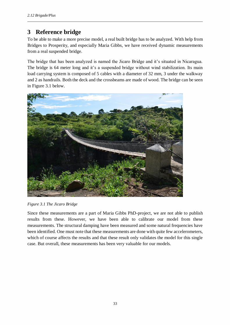
The bridge that has been analyzed is named the Jicaro Bridge and it’s situated in Nicaragua.
The bridge is 64 meter long and it’s a suspended bridge without wind stabilization. Its main
load carrying system is composed of 5 cables with a diameter of 32 mm, 3 under the walkway
and 2 as handrails. Both the deck and the crossbeams are made of wood. The bridge can be seen
in Figure 3.1 below.
Figure 3.1 The Jicaro Bridge
Since these measurements are a part of Maria Gibbs PhD-project, we are not able to publish
results from these. However, we have been able to calibrate our model from these
measurements. The structural damping have been measured and some natural frequencies have
been identified. One must note that these measurements are done with quite few accelerometers,
which of course affects the results and that these result only validates the model for this single
case. But overall, these measurements has been very valuable for our models.

2.12 Brigade/Plus
34

4.1 Evaluation of sag
35
4 Analysis of the single cable
4.1 Evaluation of sag The dynamic behavior of a suspended bridge is very affected by its sag. In some literature, for
example (Schnetzer, 2002), the natural frequencies for a suspended bridge is plotted against the
length of its span with a fixed sag/span-ratio. An example of this, made with hand calculations,
can be seen in Figure 4.1.
Figure 4.1 Natural in-plane frequencies for a single cable with a sag of L/20
When looking at Figure 4.1, it’s easy to get the impression that the natural frequencies of the
cable varies with the length of the cable. This is partly true, but the most contributing factor to
the reduction of the natural frequencies is the increasing sag of the cable due to the fixed
sag/span-ratio, i.e when the span increases, the sag of the cables also increases.
In Figure 4.2 below, a cable with a fixed sag of 5 meter has been analyzed, also this time with
hand calculations. The figure clearly shows that it is only the symetric in-plane frequencies that
changes when the span increases. The assymetric in-plane frequencies, and also all the out of
plane frequencies which aren’t showed in the figure, doesn’t change with the span length.
0,0
0,5
1,0
1,5
2,0
2,5
3,0
50 75 100 125 150
Freq
uen
cy (H
z)
Span length (m)
Natural in-plane frequencies for a single cable with a sag of L/20
1st 2nd 3rd 4th 5th 6th

4.1 Evaluation of sag
36
Figure 4.2 In-plane natural frequencies for a single cable with a fixed sag of 5 meter
When the span is shorter than 100 meter, the cable behaves just like the sagging cable it is, but
when the span length increases it behaves more and more like a taunt string. The crossover-
point for the 4th symetric- and assymetric frequencies take place at around 115 meter. The
crossover-points for higher frequencies will take place at smaller spans, but the mode shapes
for these frequencies are so small so they are not considered relevant for this report. The
remaining crossover-points happens at 130, 160 and 220 meters.
As described in the chapter Dynamics of cables, these crossover-points and the order of the
natural modes depends on the value of 𝑃𝑔𝑒
𝑃𝑔𝑒 = (8 ∙ 𝑓
𝐿)
3
∙𝐸 ∙ 𝐴
𝑔𝑎 ∙ 𝑚 ∙ 𝐿
(4.1)
Where 𝑓 is the sag of the cable
𝐸 is the Young’s modulus of the cable
𝐴 is the cross sectional area of the cable
𝑔𝑎 is the acceleration due to gravity
𝑚 is the mass per unit length of the string
𝐿 is the length between the supports
0,0
0,5
1,0
1,5
2,0
2,5
50 75 100 125 150 175 200 225 250 275 300 325 350 375 400
Freq
uen
cy (H
z)
Span length (m)
In-plane natural frequencies for a single cable with a fixed sag of 5 meter
1 Assymetric 1 Symmetric 2 Assymetric 2 Symmetric
3 Assymetric 3 Symmetric 4 Assymetric 4 Symmetric

4.1 Evaluation of sag
37
Figure 4.3 Order of the in-plane natural frequencies depending on Pge
The relationship between 𝑃𝑔𝑒 and the order of the natural in-plane frequencies can be seen in
Figure 4.3. This figure is made with the equations from (Irvine, 1981) which were presented in
the chapter Dynamics of cables. Figure 4.3 confirms the theory given in Figure 2.16 and it also
shows the next two crossover-points. The multiplier on the vertical axis in Figure 4.3 can be
used in equation (4.2).
𝑓𝑟𝑒𝑞𝑢𝑒𝑛𝑐𝑦 =𝑀𝑢𝑙𝑡𝑖𝑝𝑙𝑖𝑒𝑟
2 ∙ 𝐿√
𝐻
𝑚 𝐻𝑧
(4.2)
Where 𝐻 is the horizontal force component in the cable
𝑚 is the mass per unit length of the string
𝐿 is the length between the supports
Since the span length 𝐿 is present in both the denominator and the numerator (𝐿2 is included in
𝐻) in equation (4.2), the frequency for the symmetric modes won’t change, due to their constant
multiplier, if the length of the span varies.
A more efficient way to manipulate the natural in-plane frequencies is to change the sag of the
cable. The relationship between the frequencies and the sag can be seen in Figure 4.4, Figure
4.5 and Figure 4.6. In these figures the span length is fixed and the sag is varying which means
that all the natural frequencies, in-plane and out of plane, will be affected by the changes in the
sag. In Figure 4.4 the symmetric in-plane natural frequencies can be seen. The sign of the
0
1
2
3
4
5
6
7
8
9
10
4,9 11,6 20,0 39,0 76,2 180,6 312,0 609,5 1444,6 4875,7 39005,2
Mu
ltip
lier
Value of Pge
Order of the in-plane natural frequencies depending on Pge
1st Symmetric 1st Assymetric 2nd Symmetric 2nd Assymetric
3rd Symmetric 3rd Assymetric 4th Symmetric 4th Assymetric

4.1 Evaluation of sag
38
derivative for the symmetric frequency-curves isn’t constant since their “multiplier” is affected
by the value of 𝑃𝑔𝑒 . This is not the case for the asymmetric in-plane
Figure 4.4 Symmetric in-plane natural frequencies for a single cable with span L=150 meter
frequencies. The sign of the derivative is always constant, i.e. if the sag increases the
frequencies will always decrease. This can be seen in Figure 4.5 below.
Figure 4.5 Asymmetric in-plane natural frequencies for a single cable with span L=150 meter
0,0
0,5
1,0
1,5
2,0
2,5
3,0
3,5
4,0
4,5
L/100 L/75 L/50 L/30 L/20 L/10 L/5
Freq
uen
cy (H
z)
Sag
Symmetric in-plane natural frequencies for a single cable with span L=150 meter
1st 2nd 3rd 4th 5th
0,0
0,5
1,0
1,5
2,0
2,5
3,0
3,5
4,0
4,5
5,0
L/100 L/75 L/50 L/30 L/20 L/10 L/5
Freq
uen
cy (H
z)
Sag
Asymmetric in-plane natural frequencies for a single cable with span L=150 meter
1st 2nd 3rd 4th 5th

4.1 Evaluation of sag
39
The first three symmetric and three antisymmetric in-plane frequencies have been plotted
together in Figure 4.6. This figure clearly shows three crossover-points on the way from
behaving like a taut string at a sag of L/100 to having like a sagging cable from sag bigger than
L/20.
Figure 4.6 In-plane natural frequencies for a single cable with span L=150 meter
Since it’s quite easy to calculate the natural frequencies for a single cable, it would be useful if
theses frequencies corresponds to the one that’s been calculated from the bridge models in
Brigade/Plus. This connection will be researched further in chapter 0.
0,00
0,50
1,00
1,50
2,00
2,50
3,00
L/100 L/75 L/50 L/30 L/20 L/10 L/5
Freq
uen
cy (H
z)
Sag
In-plane natural frequencies for a single cable with span L=150 meter
1st Symmetric 1st Assymetric 2nd Symmetric
2nd Assymetric 3rd Symmetric 3rd Assymetric

4.2 Modelling of a single cable in Brigade/Plus
40
4.2 Modelling of a single cable in Brigade/Plus As a first step in the modelling of a suspended bridge, a single cable has been modelled. Since
it has been shown in chapter 2.7 that it’s easy to calculate the natural frequencies by hand, this
is a good way to start working with Brigade since it’s possible to compare the result from the
model with the hand calculated results. This is a good way to check if the results from the model
is reasonable. The chosen cable has the diameter of 35 mm which gives an approximate metallic
area of 544 mm2. A rough sketch of the cable can be seen in Figure 4.7 below.
Length L: 60 meter
Sag f: 3 meter
Mass: 4.27 kg/m
E-modulus: 110 GPa
Metallic area: 544 mm2
The cable in the model is composed of two node beam elements and it’s pinned in both ends.
Figure 4.8 Brigade model
The Brigade model can be seen in Figure 4.8 above. The cable force near the supports in the
model is 6,37 kN. Since the sag is increased in the cables deformed stadium and the hand
calculation estimate the cable force to be 6.41 kN it’s seem like a reasonable result.
The eigenmodes and appurtenant frequencies have been calculated for both in plane- and out
of plane vibrations. Since the 𝑃𝑔𝑒-number is quite high, 𝑃𝑔𝑒 ≈ 1500, the cable will act like a
sagging cable (which it is) and not like a taut string or anything in between. This causes the first
vertical eigenmode to be assymetric, which both the hand calculations and the Brigade model
has shown. As seen in the tables below, the frequencies calculated by hand and the ones
calculated in the model are very alike.
Figure 4.7 Sketch of the cable
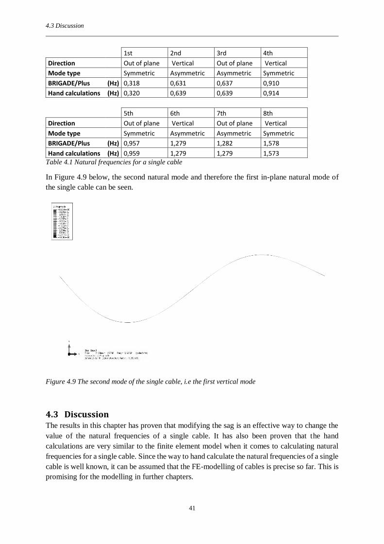
4.3 Discussion
41
1st 2nd 3rd 4th
Direction Out of plane Vertical Out of plane Vertical
Mode type Symmetric Asymmetric Asymmetric Symmetric
BRIGADE/Plus (Hz) 0,318 0,631 0,637 0,910
Hand calculations (Hz) 0,320 0,639 0,639 0,914
5th 6th 7th 8th
Direction Out of plane Vertical Out of plane Vertical
Mode type Symmetric Asymmetric Asymmetric Symmetric
BRIGADE/Plus (Hz) 0,957 1,279 1,282 1,578
Hand calculations (Hz) 0,959 1,279 1,279 1,573 Table 4.1 Natural frequencies for a single cable
In Figure 4.9 below, the second natural mode and therefore the first in-plane natural mode of
the single cable can be seen.
Figure 4.9 The second mode of the single cable, i.e the first vertical mode
4.3 Discussion The results in this chapter has proven that modifying the sag is an effective way to change the
value of the natural frequencies of a single cable. It has also been proven that the hand
calculations are very similar to the finite element model when it comes to calculating natural
frequencies for a single cable. Since the way to hand calculate the natural frequencies of a single
cable is well known, it can be assumed that the FE-modelling of cables is precise so far. This is
promising for the modelling in further chapters.

4.3 Discussion
42

5.1 Hand calculations
43
5 Static analysis of the suspended bridge
5.1 Hand calculations Designing a suspended bridge with regard to only static loads isn’t a difficult task for a person
with some knowledge of structural engineering. The design procedure can be made systematic
which has led to the creation of a design guide in the form of an Excel sheet. The Excel sheet
can be used to design a suspended bridge according to both Helvetas and Eurocode and also
with or without windguys as lateral stabilization. Since the main and handrail cables in a
suspended bridge are the structural members that carries the whole load of the bridge and its
users, the main focus in the design guide is to determine the appropriate dimensions for these
cables. A design example for a 150 meter long suspended bridge made with this design guide
can be seen in the appendix.
Note that unless otherwise stated, all hand calculations presented are calculated with the design
guide.
5.2 Modelling Component Part Element
Cable Wire 3D deformable B31
Crossbeam Wire 3D deformable B31
Suspender Wire 3D deformable T3D2 Table 5.1 Properties for components in Brigade/Plus
B31 is a 2 node beam element in 3D space with a linear interpolation function. And T3D1 is a
2 node truss element in 3D space. This means that the connection between the suspender and
the crossbeam will be a joint due to the lack of rotational degrees of freedom in the truss
element.
5.3 Influence lines An influence line shows the deflection, moment, shear force etc for a certain position on the
bridge due to a force placed somewhere on the bridge. In this case, influence lines showing the
deflection for two points on a 150 meter long suspended bridge has been made. The bridge is
designed according to Eurocode. The two points are:
𝑥 =𝐿
2= 75 𝑚
𝑥 =𝐿
4= 37.5 𝑚.
The influence lines had been made with the Brigade/Plus model and the recorded displacements
has been normalized to achieve a displacement factor 𝜂 that can be multiplied with an acting
force on the bridge. Since the unit of 𝜂 is 𝑚/𝑁, the user of the influence line can multiply the
value of the force with the displacement factor 𝜂 for the location of the force.

5.3 Influence lines
44
One important matter to notice is the nonlinearity in the force-displacement relationship. This
nonlinearity is important to have this in mind when using the influence lines. The influence
lines in Figure 5.1 and Figure 5.2 has been made by recording the displacement due to a vertical
force with a magnitude of 100 newton.
Figure 5.1 Vertical displacements at x=75 meter
Figure 5.2 Vertical displacement at x=37,5 meter
-7E-05
-6E-05
-5E-05
-4E-05
-3E-05
-2E-05
-1E-05
0E+00
1E-05
2E-05
0 10 20 30 40 50 60 70 80 90 100 110 120 130 140 150 160
η(m
/N)
x (m)
Influence line for vertical displacement at x=75 m
Extracted with F=100 N
-8E-05
-7E-05
-6E-05
-5E-05
-4E-05
-3E-05
-2E-05
-1E-05
0E+00
1E-05
2E-05
3E-05
4E-05
0 10 20 30 40 50 60 70 80 90 100 110 120 130 140 150 160
η(m
/N)
x (m)
Influence line for vertical displacement at x=37.5 m
Extracted with F=100 N

5.3 Influence lines
45
To investigate the assumption of nonlinearity two another influence lines was made. These two
recorded the deflections due to a vertical force of 2000 newton for the same points as the earlier
ones. In Figure 5.3 and Figure 5.4 the influence lines for the force of 2000 newton has been
inserted. Both of the influence lines in each figure has been normalized and as expected a small
difference between the lines can be seen. When using the influence lines, interpolation have to
be used even if the difference between the lines isn’t big.
If one want to use the influence lines for a uniformly distributed load, the influence line have
to be integrated over the length of the uniformly distributed load. For example, if the maximum
possible displacement for the midpoint of the bridge should be determined, the influence line
should be integrated over the distance 𝑥 ≈ 43 − 𝑥 ≈ 107 and then multiplied with the
uniformly distributed load that should be placed over the same distance.
Figure 5.3 Vertical displacements at x=75 meter
-7E-05
-6E-05
-5E-05
-4E-05
-3E-05
-2E-05
-1E-05
0E+00
1E-05
2E-05
0 10 20 30 40 50 60 70 80 90 100 110 120 130 140 150 160
η(m
/N)
x (m)
Influence line for vertical displacement at x=75 m
Extracted with F=100 N
Extracted with F=2000 N

5.3 Influence lines
46
Figure 5.4 Vertical displacement at x=37,5 meter
An example of how to use an influence line can be seen below. A force with a magnitude of 1
kN has been placed at the position 𝑥 = 20 𝑚. This can be seen in Figure 5.5. The displacement
for the two positions can be calculated with interpolation between the two influence lines in
Figure 5.3 and Figure 5.4:
Deformation at 𝑥 = 37.5 𝑚: 𝑣37.5 = 1000 ∙ −3,1 ∙ 10−5 = −31 𝑚𝑚
Deformation at 𝑥 = 75 𝑚: 𝑣75 = 1000 ∙ 1,35 ∙ 10−5 = 13,5 𝑚𝑚
Figure 5.5 Deflection due to a vertical force with the position x=20 meter
-8E-05
-7E-05
-6E-05
-5E-05
-4E-05
-3E-05
-2E-05
-1E-05
0E+00
1E-05
2E-05
3E-05
4E-05
0 10 20 30 40 50 60 70 80 90 100 110 120 130 140 150 160
η(m
/N)
x (m)
Influence line for vertical displacement at x=37.5 m
Extracted with F=100 N
Extracted with F=2000 N

5.4 Displacements
47
Another example can be seen below. A force with a magnitude of 1 kN has been placed at the
position 𝑥 = 75 𝑚. This can be seen in Figure 5.6. The displacement for the two positions can
be calculated with interpolation between the two influence lines in Figure 5.3 and Figure 5.4:
Deformation at 𝑥 = 37.5 𝑚: 𝑣37.5 = 1000 ∙ 0,75 ∙ 10−5 = 7,5 𝑚𝑚
Deformation at 𝑥 = 75 𝑚: 𝑣75 = 1000 ∙ −6,0 ∙ 10−5 = −60 𝑚𝑚
Figure 5.6 Deflection due to a vertical force with the position x=75 meter
5.4 Displacements Due to their slim and flexible shape, suspended bridges can be subjected to large vertical and
lateral displacements. In this chapter, displacements due to static loads will be discussed.
Displacements in the vertical direction will always occur, in fact the dead load sag is a
displacement from the hoisting sag, i.e. the sag the cables are hoisted to during construction.
The vertical displacements for the two investigated bridges can be seen in Table 5.2.
The vertical displacements for the 150 meter long bridge have been determined with Brigade,
influence lines and hand calculations. The live load used is the characteristic live load according
to Eurocode for a 150 meter long bridge, and this load acts on the whole length of the bridge.
The calculated displacements are quite similar and they span from 1,6 – 1,75 meter, which
seems like a reasonable result. These displacements won’t significantly affect the users of the
bridge, with a possible exception for old or disabled people. However, live loads of this
magnitude are extremely rare. For a smaller but still large live load, 1000 kN/m, the vertical
displacement becomes approximately 0,78 meter.
Span Dead load Live load Total load Displacement
Vertical (m) (N/m) (N/m) (N/m) (m)
Brigade 150 460 2670 3137 1,65
influence line 150 460 2670 3137 1,6
Hand calculations 150 460 2670 3137 1,75
Brigade 64 490 2670 3167 0,36
Hand calculations 64 490 2670 3167 0,33 Table 5.2 Vertical displacements

5.4 Displacements
48
The deformed shape of the 150 meter long bridge can be seen in Figure 5.7 below.
Figure 5.7 Vertical displacements due to a live load of 2,67 kN/m.
Lateral displacements due to wind load are hard to determine in a realistic way. Due to the non-
steady state of wind loads, static displacements are more an easy calculated estimation of
possible lateral displacements. More lateral displacements due to wind will be presented in the
dynamics chapter 0
The lateral displacements in Table 5.3 below are based on wind speeds of 10, 15 and 20 m/s
and the wind loads are determined according to equation (2.31. For both the Brigade and the
hand calculations, the bridge has only been subjected to its own dead load since this will be the
worst case with regard to lateral displacements. Live load would have increases the reference
area for the wind load, but since the vertical load is greater than the increased wind load, this
would have reduced the lateral displacements.
Span Windguys Wind Dead load Wind load Displacement
Lateral (m) (m/s) (N/m) (N/m) (m)
Brigade 150 - 10 460 57 0,99
Brigade 150 Yes 10 460 57 0,18
Hand calculations 150 - 10 460 57 0,92
Brigade 150 - 15 460 129 2,16
Brigade 150 Yes 15 460 129 0,34
Hand calculations 150 - 15 460 129 2,01
Brigade 150 - 20 460 229 3,55
Brigade 150 Yes 20 460 229 0,51
Hand calculations 150 - 20 460 229 3,32
Table 5.3 Lateral displacements
As it can be seen in Table 5.3, the lateral displacements determined with Brigade and hand
calculations are very similar. The hand calculations are done with the “pendulum theory”
presented in chapter 2.10.5. The lateral displacements determined with the Brigade model

5.5 Stress distribution
49
without windguys are approximately 7% bigger than the displacements determined by the hand
calculations. It can therefore be stated that quite simple hand calculations are very similar to
finite element models when calculating lateral displacement due to static wind load for bridges
without windguys.
The lateral displacements due to a wind speed of 20 m/s for the 150 meter long bridge with and
without windguys can be seen in Figure 5.8 below.
Figure 5.8 Lateral displacements due to a static wind of 20 m/s
Figure 5.9 Lateral displacements due to a static wind of 20 m/s
5.5 Stress distribution The main part of the loads on a suspended bridge acts on the walkway deck. If this load shall
be uniformly distributed over both the walkway cables and the handrail cables, the suspenders
have to be very stiff. Since the suspenders, and therefore the connection, between the handrail

5.5 Stress distribution
50
and walkway cables aren’t completely stiff, there will be a difference between the forces in
these cables.
To be able to investigate the force and the appurtenant stress distribution in the cables, both the
models of the Jicaro Bridge and the 150 meter bridge have been analyzed. The cable diameter
of the Jicaro Bridge in the model has in this case been changed to a diameter that’s
recommended by Eurocode. The comparison between the two bridges would otherwise have
been poor.
The two bridge models have been subjected to both their design load and their dead load and
the stresses in the cables have been measure for these load cases. An additional load step was
used for the Jicaro Bridge, which can be seen in Figure 5.10. In this figure, two lines can be
seen. The upper line corresponds to the stress in one of the walkway cables and the lower line
corresponds to the stress in one of the handrail cables. The stress is plotted against time, where
the dead load was applied in steps during the first second and the 1 kN/m load was applied in
steps during the second second.
The stress difference starts during the first load steps. Since most of the dead load are situated
in the lower parts of the bridge, the stress in the walkway cables will increase first. Since the
handrail cables are connected with suspenders to the walkway cables, a vertical displacement
of the walkway cables must occur before the suspenders will be tensioned and the lower part of
the bridge starts to “hang” in the handrail cables. So if the suspenders aren’t pre-tensioned,
which seems hard to achieve, the deformation and therefore the stresses on the walkway cables
will be greater, at least for small loads.
Figure 5.10 Stress distribution for walkway cables and handrail cables for the Jicaro Bridge
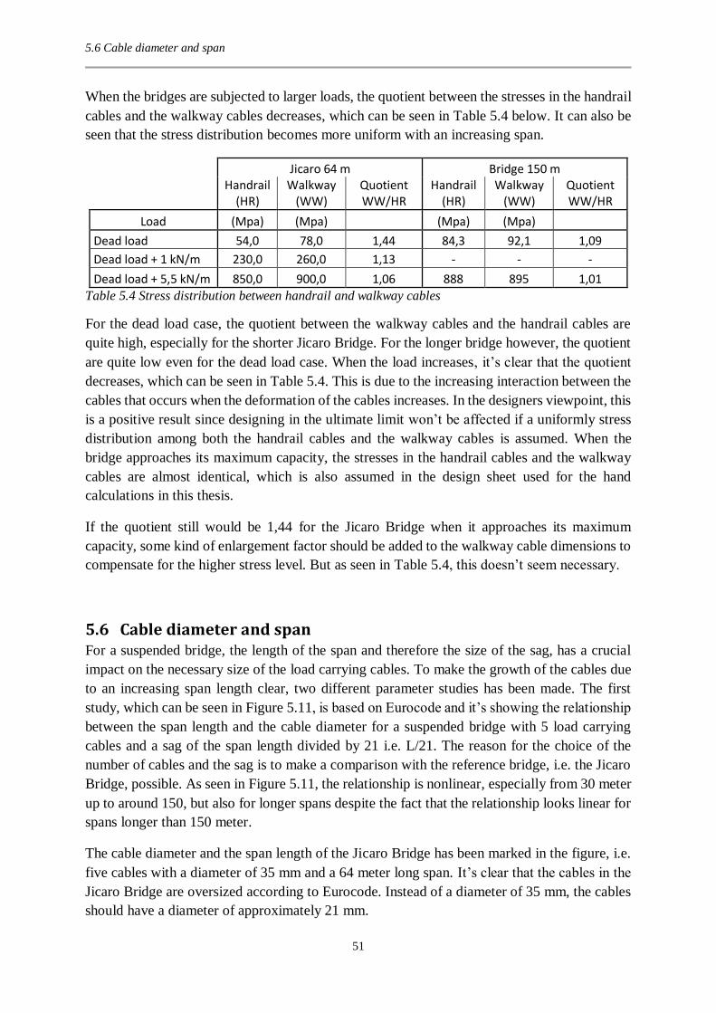
5.6 Cable diameter and span
51
When the bridges are subjected to larger loads, the quotient between the stresses in the handrail
cables and the walkway cables decreases, which can be seen in Table 5.4 below. It can also be
seen that the stress distribution becomes more uniform with an increasing span.
Jicaro 64 m Bridge 150 m
Handrail
(HR) Walkway
(WW) Quotient WW/HR
Handrail (HR)
Walkway (WW)
Quotient WW/HR
Load (Mpa) (Mpa) (Mpa) (Mpa)
Dead load 54,0 78,0 1,44 84,3 92,1 1,09
Dead load + 1 kN/m 230,0 260,0 1,13 - - -
Dead load + 5,5 kN/m 850,0 900,0 1,06 888 895 1,01 Table 5.4 Stress distribution between handrail and walkway cables
For the dead load case, the quotient between the walkway cables and the handrail cables are
quite high, especially for the shorter Jicaro Bridge. For the longer bridge however, the quotient
are quite low even for the dead load case. When the load increases, it’s clear that the quotient
decreases, which can be seen in Table 5.4. This is due to the increasing interaction between the
cables that occurs when the deformation of the cables increases. In the designers viewpoint, this
is a positive result since designing in the ultimate limit won’t be affected if a uniformly stress
distribution among both the handrail cables and the walkway cables is assumed. When the
bridge approaches its maximum capacity, the stresses in the handrail cables and the walkway
cables are almost identical, which is also assumed in the design sheet used for the hand
calculations in this thesis.
If the quotient still would be 1,44 for the Jicaro Bridge when it approaches its maximum
capacity, some kind of enlargement factor should be added to the walkway cable dimensions to
compensate for the higher stress level. But as seen in Table 5.4, this doesn’t seem necessary.
5.6 Cable diameter and span For a suspended bridge, the length of the span and therefore the size of the sag, has a crucial
impact on the necessary size of the load carrying cables. To make the growth of the cables due
to an increasing span length clear, two different parameter studies has been made. The first
study, which can be seen in Figure 5.11, is based on Eurocode and it’s showing the relationship
between the span length and the cable diameter for a suspended bridge with 5 load carrying
cables and a sag of the span length divided by 21 i.e. L/21. The reason for the choice of the
number of cables and the sag is to make a comparison with the reference bridge, i.e. the Jicaro
Bridge, possible. As seen in Figure 5.11, the relationship is nonlinear, especially from 30 meter
up to around 150, but also for longer spans despite the fact that the relationship looks linear for
spans longer than 150 meter.
The cable diameter and the span length of the Jicaro Bridge has been marked in the figure, i.e.
five cables with a diameter of 35 mm and a 64 meter long span. It’s clear that the cables in the
Jicaro Bridge are oversized according to Eurocode. Instead of a diameter of 35 mm, the cables
should have a diameter of approximately 21 mm.

5.6 Cable diameter and span
52
Figure 5.11 Cable diameter according to Eurocode for a bridge with a sag of L/21
A more obvious method to describe the relationship between the span length and the cable size
is to use the metallic cross-sectional area instead of the cable diameter, which can be seen in
Figure 5.12. The metallic cross-sectional area are direct proportional to the total strength of the
cables and it’s approximately 55-56 % of the total cross-sectional area of the type of wire rope
used in this report. The cables use in the Eurocode design is of rope class 1570 MPa, with 𝑓𝑢 =
1570 𝑀𝑃𝑎 and 𝑓0.2 = 1370 𝑀𝑃𝑎.
In Figure 5.12 it’s even clearer that the Jicaro Bridge are oversized according to Eurocode. The
metallic cross-sectional area of the Jicaro Bridge is almost three times bigger than the necessary
area suggested by Eurocode.
Figure 5.12 Metallic cross-sectional area according to Eurocode for a bridge with a sag of L/21

5.6 Cable diameter and span
53
The other bridge marked in Figure 5.12 is the Trift Bridge, which is a suspended bridge
spanning over a gorge close to the Trift glacier in Switzerland. This bridge was opened in 2009
when it replaced a few year older bridge that suffered from wind instability. The Trift Bridge
has a similar sag ratio and it’s design for a similar load as the load recommended by Eurocode
(Pfaffen, Brog, & Van Rooden, 2009). As seen in Figure 5.12, the dimension of the cables in
the Trift Bridge are slightly bigger but still close to the dimensions recommended by Eurocode.
One reason for the bigger dimension can be the Trift Bridge are fitted with pre-tensioned
windguys which creates an extra vertical force since the windguys aren’t completely horizontal.
Another reason for using the metallic cross-sectional area as unit for the relationship between
span length and cable size is that a comparison between the Jicaro Bridge and the dimensions
suggested by Helvetas is possible. When using the Helvetas design guide it recommends
different cable combinations depending on the size of the calculated force. Since the number
and diameter of the cables used in these combinations varies, it’s impossible to use the cable
diameter as unit for the cable size. However, the metallic cross-sectional area for each cable
combination is given which makes a comparison possible. In Figure 5.13 below, a maximum
span for each cable combination has been calculated.
Even according to Helvetas, the cables in the Jicaro Bridge seems to be oversized. If the Jicaro
Bridge should have been designed according to Helvetas, the recommended cable combination
should have been point number three in the line in Figure 5.13 below, i.e. 4 cables with a
diameter of 26 mm under the walkway and 2 cables with a diameter of 26 mm as handrails.
This gives a metallic cross-sectional area of 1751 mm2 even if approximately 1500 mm2 is
necessary.
The cables in the Trift Bridge are undersized according to Helvetas. Since the dimension of the
cables where close to the Eurocode dimensions, this result was expected.
Figure 5.13

5.7 Discussion
54
Not surprisingly, the curves in Figure 5.12 and Figure 5.13 has a quite constant factor between
them, which can be seen in Figure 5.14. The areas calculated according to Helvetas are
approximately 60 % bigger than the areas calculated according to Eurocode. However, for a
span of 64 meter, both these areas are much smaller than the metallic cross-sectional area of the
cables in the Jicaro Bridge. The Trift Bridge positions itself between the Helvetas- and the
Eurocode curves. Its metallic cross-sectional area is approximately 400 mm2 bigger than the
Eurocode recommendations and 1000 mm2 smaller than the Helvetas recommendation.
Note that neither the Helvetas nor the Eurocode curves are calculated with regard to windguys.
Figure 5.14
5.7 Discussion The influence lines are a good tool to identify the most crucial load positions for a suspended
bridge but they should be used with care. The influence lines presented in chapter 5.3 are created
specifically for a 150 meter long bridge designed according to Eurocode and the displacement
axis should only be used for this bridge. However, the shape of the influence lines won’t differ
much from bridges with different span but with the same span/sag-ratio. They can therefore be
used with quite good accuracy to determine the displacements for different load positions.
The stress distribution between the handrail and walkway cables showed to be more and more
uniformly distributed when the vertical load was increased, i.e. the cables deforms uniformly.
The interaction between the handrail and the walkway cables depends on the suspenders
connecting them. The difference between the vertical deformations, and therefore the stresses,
in the cables will decrease with an increasing load. Since the stresses in the cables are almost
similar when the bridge reaches its structural capacity, the design in the ultimate limit state can
be made with the assumption of full interaction between the cables.

5.7 Discussion
55
Hand calculations have proved to be very alike the Brigade-calculations when it comes to
displacements due to static loads. The need for time-consuming FEM-models is therefore small
when only static loads are used in the design.
The design according to Helvetas must be seen as oversized in comparison with Eurocode since
the recommended cable dimensions by Helvetas are approximately 60 % larger than the
recommended dimensions by Eurocode. Bridges to Prosperitys design guide is based on the
Helvetas design guide, but as it can be seen in Figure 5.14, the design of the Jicaro Bridge is
very oversized according to both Helvetas and Eurocode. The cross-sectional area of the cables
in the Jicaro Bridge is almost identical with the over 100 meter longer Trift Bridge even if the
cable quality can differ between them. It’s however determined that damage due to fatigue
aren’t common on suspended bridges designed according to Helvetas (Schnetzer, 2002). If this
is because of the larger dimensions will remain uncertain, but it’s clear that the larger
dimensions aren’t a disadvantage when it comes to reducing fatigue damage.
The available cables sizes on the building site must also be considered in the design. Perhaps
it’s cheaper to buy a larger cable dimension on site than transport a smaller cable a long way.
This could be one reason to the oversized design of the Jicaro Bridge. Since it’s only the
walkway and handrail cables that are the main load carrying elements, it’s quite cheap to
increase the cable size and therefore the structural capacity of the bridge.

5.7 Discussion
56

6.1 Modal superpositioning
57
6 Dynamic Analysis
6.1 Modal superpositioning
6.1.1 Natural Frequencies The extracting of the natural frequencies is done both by hand calculation for a single cable and
it’s also treated as an eigenvalue problem in Brigade/plus. The step in Brigade that is used is a
linear perturbation step called frequency. When the whole bridge is modelled one can obtain
torsion modes in addition to vertical and out of plane modes. The number of natural frequencies
and modes extracted is user defined but in theory it’s possible to extract a number equal to the
number of degrees of freedom. 3 vertical, out of plane and torsional frequencies are extracted
both from the Jicaro Bridge and the 150 m span bridge. A few different modes are presented
below while the rest can be seen in appendix.
Figure 6.1 First out of plane mode shape for the Jicaro Bridge
Figure 6.2 Second out of plane mode shape for the Jicaro Bridge

6.1 Modal superpositioning
58
Figure 6.3 First in- plane mode shape for the Jicaro Bridge
Figure 6.4 First torsional mode shape for the 150 meter span bridge
A comparison between hand calculated and FEM modelled frequencies has been done. The
frequencies from these calculations can be seen in Table 6.1 below.

6.1 Modal superpositioning
59
Jicaro Bridge Single cable Modelled bridge Single cable
64 meter 64 meter 150 meter 150 meter
Natural frequencies Brigade/Plus Hand calculated Brigade/Plus Hand calculated
Out of plane (Hz) (Hz) (Hz) (Hz)
1st 0,318 0,320 0,201 0,209
2nd 0,608 0,639 0,388 0,419
3rd 0,910 0,959 0,567 0,628
In-plane
1st 0,620 0,639 0,401 0,419
2nd 0,887 0,911 0,563 0,592
3rd 1,249 1,279 0,805 0,837 Table 6.1 Comparison of natural frequencies calculated by FEM-models and by hand
Note that the bridges in the Brigade/Plus-models are subjected to their own dead load, i.e. the
weight from cables, suspenders, crossbeams etc. The single cables are only subjected to the
dead load of the cable itself.
6.1.2 Excitation / Impulse To analyse the dynamic response of the bridges, energy need to be added to the system.
Consequently the response will be very much dependent on the energy added. The excitation
of the bridge in the horizontal direction is based on the wind velocities of 10, 15 and 20 m/s.
Since “real” wind loads are very difficult to model, a reference method is used where the load
is applied as a line load on the side of the bridge in the out of plane direction. The load is built
up under a 2 second period and then decayed under a period of 0.1 second. This will allow free
vibration of the bridges in the excited modes when load has decayed to zero. The load is applied
with Smooth Step in Brigade. This gives the transition between the input values of the amplitude
as a fifth degree polynomial. The first and second derivative will be zero at the start and end
value. Figure 6.5 shows the transition of the load between two input values.
Figure 6.5 Amplitude curve for Smooth Step

6.2 Modal analysis
60
6.1.3 Damping The Rayleigh damping coefficients are extracted from experimental dynamic pluck tests on the
Jicaro Bridge in Nicaragua. The pluck tests are performed by Bridges to Prosperity and Maria
Gibbs. According to (Austrell, 2015) the damping ratio on lightly damped systems can be given
by equation (6.1).
6.2 Modal analysis In Brigade the modal super positioning analysing step is a linear perturbation step called modal
dynamics. This step needs to be preceded by the frequency step where the natural frequencies
are extracted. The number of natural frequencies used for the modal analysis is set to 25.
Because of the excitation of the bridges is done along the whole span, one can suspect that the
dominant mode will be the first mode in the out of plane direction, see Figure 6.1. The results
extracted from the analyses will be displacements and accelerations for the midpoints of the
three bridges, Jicaro Bridge (64 m), 150 m span bridge and 150 m span bridge with windguys
installed.
6.2.1 Displacements The response in the form of displacements is shown in Figure 6.6, Figure 6.7 and Figure 6.8.
Each figure shows the response from the three different wind velocities acting on one of the
bridges.
Figure 6.6 Lateral displacement in the center of Jicaro Bridge
-1,2-1,1
-1-0,9-0,8-0,7-0,6-0,5-0,4-0,3-0,2-0,1
00,10,20,30,40,50,60,70,80,9
0 1 2 3 4 5 6 7 8 9 10 11 12 13 14 15 16 17 18 19 20 21 22 23
Dis
pla
cem
ents
(m
)
Time (s)
Lateral Displacement Jicaro Bridge (64 m)
10 m/s
15 m/s
20 m/s
𝜉 =1
2πj∙ ln (
𝑢𝑖
𝑢𝑖+𝑗)
(6.1)

6.2 Modal analysis
61
Figure 6.7 Lateral displacement in the center of the 150 m span bridge
Figure 6.8 Lateral displacement in the center of the 150 m span bridge with windguys
-2,8-2,6-2,4-2,2
-2-1,8-1,6-1,4-1,2
-1-0,8-0,6-0,4-0,2
00,20,40,60,8
11,21,41,61,8
22,2
0 1 2 3 4 5 6 7 8 9 10 11 12 13 14 15 16 17 18 19 20 21 22 23
Dis
pla
cem
ents
(m
)
Time (s)
Lateral Displacements 150 span bridge
10 m/s
15 m/s
20 m/s
-1,3-1,2-1,1
-1-0,9-0,8-0,7-0,6-0,5-0,4-0,3-0,2-0,1
00,10,20,30,40,50,60,70,80,9
11,11,2
0 1 2 3 4 5 6 7 8 9 10 11 12 13 14 15 16 17 18 19 20 21 22 23 24 25
Dis
pla
cem
ents
(m
)
Time (s)
Lateral Displacements 150 m span bridge with windguys
10 m/s
15 m/s
20 m/s

6.2 Modal analysis
62
6.2.2 Accelerations The response in the form of accelerations is shown in Figure 6.9, Figure 6.10 and Figure 6.11.
Each figure shows the response from the three different wind velocities acting on one of the
bridges.
Figure 6.9 Lateral accelerations in the center of Jicaro Bridge
-8
-7
-6
-5
-4
-3
-2
-1
0
1
2
3
4
5
6
7
8
9
0 1 2 3 4 5 6 7 8 9 10 11 12 13 14 15 16 17 18 19 20 21 22 23
Acc
eler
atio
ns
(m/s
2)
Time (s)
Lateral accelerations Jicaro Bridge (64 m)
10 m/s
15 m/s
20 m/s
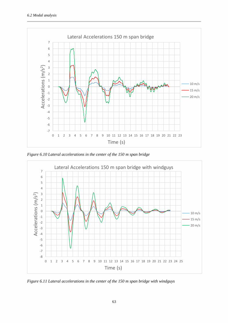
6.2 Modal analysis
63
Figure 6.10 Lateral accelerations in the center of the 150 m span bridge
Figure 6.11 Lateral accelerations in the center of the 150 m span bridge with windguys
-7
-6
-5
-4
-3
-2
-1
0
1
2
3
4
5
6
7
0 1 2 3 4 5 6 7 8 9 10 11 12 13 14 15 16 17 18 19 20 21 22 23
Acc
eler
atio
ns
(m/s
2)
Time (s)
Lateral Accelerations 150 m span bridge
10 m/s
15 m/s
20 m/s
-8
-7
-6
-5
-4
-3
-2
-1
0
1
2
3
4
5
6
7
0 1 2 3 4 5 6 7 8 9 10 11 12 13 14 15 16 17 18 19 20 21 22 23 24 25
Acc
eler
atio
ns
(m/s
2)
Time (s)
Lateral Accelerations 150 m span bridge with windguys
10 m/s
15 m/s
20 m/s

6.3 Implicit dynamic step
64
6.3 Implicit dynamic step As stated before the cables gives a nonlinearity to the problem. And because a modal analysis
only can handle linear problems a comparison is made with an implicit dynamic analysis. The
comparison is made on the 150 meter span bridge without windguys and a wind velocity of 10
m/s. It should also be noted that the modal analysis only uses the first 25 modes which also can
give a deviation between the different analyses. The response comparison in the form of
displacements and accelerations are shown in the figures below.
Figure 6.12 Lateral displacement comparison between modal and implicit dynamic analysis
-1,2
-1
-0,8
-0,6
-0,4
-0,2
0
0,2
0,4
0,6
0,8
0 1 2 3 4 5 6 7 8 9 10 11 12 13 14 15 16 17 18 19 20 21 22 23 24 25
Dis
pla
cem
ents
(m
)
Time (s)
Lateral displacement comparison Modal and Implicit Dynamic analysis
10 m/s Modal
10 m/s Implicit

6.4 Discussion
65
Figure 6.13 Lateral accelerations comparison between modal and implicit dynamic analysis
6.4 Discussion One must first mention that hand calculations and FE-models aren’t the only way to identify
the dynamic behavior of bridges. Wind tunnel tests are still in use when designing larger bridges
since computer models haven’t replaced this method as a way of identifying the dynamic
behavior. This fact must be considered with respect.
The natural frequencies that are extracted from Brigade seems to conform with the hand
calculations for a single cable with the same sag and span and only its own self weight acting
on it. This means that hand calculations is a good way to approximate the first few natural
frequencies in the in-plane and out of plane directions for this type of bridges without the need
to use more advanced FE-models. With the Brigade model, torsional modes can be identified
which can be useful if further investigation is done on wind effects. One conclusion of this
chapter is that a good way to affect the natural frequencies of a suspended bridge is to modify
the size of its sag.
The response for different type of bridges follows its first out of plane frequency. The
displacement of the midpoint increases with a larger span which also has been concluded in
chapter 5.4. With windguys installed the displacement again decreases. The acceleration peak
values on the other hand decreases with a larger span but seems to be unchanged with or without
-2
-1
0
1
2
0 1 2 3 4 5 6 7 8 9 10 11 12 13 14 15 16 17 18 19 20 21 22 23 24 25
Acc
eler
atio
ns
(m/s
2)
Time (s)
Lateral acceleration comparison Modal and Implicit dynamic analysis
10 m/s Modal
10 m/s Implicit

6.4 Discussion
66
the windguys. One can make the conclusion that the design criteria for using windguys is based
on allowed lateral displacement rather than allowed accelerations of the bridge.
The acceleration values for the three bridge types are relative large compared to the suggested
accelerations by Nakamura. The choice of excitation parameters that are put into the system is
of great importance for the response of the bridge and will greatly influence the values. It’s
possible that it’s more important in this case to analyse the change in behavior with greater span
and windguys rather than analysing the actual peak values.
In the comparison between a modal analysis and an implicit analysis in Figure 6.12 and Figure
6.13, a difference can be distinguished in the early peak values for the displacements. The
implicit analysis gives larger displacements than the modal analysis. The peak values for the
accelerations seems to conform in a better way. A small difference in frequency of the response
can also be seen. The modal analysis gives overall a good approximation of the response of the
bridge but to fully analyse the nonlinearities that occur with cables, an implicit analysis is
needed. Note that the modal analysis requires less calculation time than the implicit dynamic
analysis.

6.4 Discussion
67
7 Conclusions Since all the results have been discussed in each chapter, this chapter will summarize them
shortly.
Modifying the sag is the best way to affect the natural frequencies.
The Brigade model and hand calculations gives very alike result for both vertical and lateral
displacements due to static loads.
The stress distribution between the handrail and the walkway cables is not a problem for
designing in ultimate limit state. The stress distribution becomes more uniformly distributed
between the cables when the vertical load increases, i.e. the cables will deform uniformly.
When analyzing the natural frequencies of a suspended bridge, a good approximation will be
to evaluate a single cable with the same sag and span subjected to its self weight.
The criteria for using windguys should rather be based on displacements than accelerations. It
could also be a combination of the two.
In Brigade/plus the cables, and therefore the whole bridge, will have no stiffness before the
dead load is applied which means that the sag will get larger than what it’s initially modeled
as. This needs to be accounted for when modelling a suspended bridge in Brigade/plus.
Bridges designed with design guides from Helvetas and Bridges to Prosperity requires larger
cable dimensions compared with bridges designed according to Eurocode.
When determining the lateral dynamic response from wind loads, a modal dynamics analysis
gives a good approximation of the behavior of the bridge. However, a full implicit dynamic
analysis is preferred.

7.1 Further investigations
68
7.1 Further investigations In this section a number of suggestions are made for further investigations and analyses that
have not been included in this thesis.
More full dynamic implicit analyses should be done to fully understand the nonlinear
behavior of the dynamic response.
If possible make experimental tests on existing suspended bridges for calibrating
models. This can for instance be a simple pluck test to identify natural frequencies.
Try to find a criteria depending on displacements, accelerations and span length for
when windguys should be installed.
The effect of temperature changes. Very low temperature will lead to a temporary
shortening of the cables which will increase the stress levels.
Corrosion protection of the cables.

7.1 Further investigations
69
8 References Austrell, P. E. (2015, 06 08). VSMN10 Strukturdynamiska Beräkningar. Retrieved from
VSMN10 Strukturdynamiska Beräkningar:
http://www.byggmek.lth.se/fileadmin/byggnadsmekanik/SDOF_with_damping_mod.p
df
BBC. (2015, 11 7). BBC. Retrieved from BBC: http://www.bbc.com/news/magazine-
33291373
Certex. (n.d.). Certex. Retrieved 01 29, 2015, from Certex:
http://www.certex.co.uk/steelwirerope/steelwireropes/technicalinformation/properties-
of-extension-of-steel-wire-ropes
COWI. (2015, 05 18). COWI. Retrieved from COWI:
http://www.cowi.com/menu/NewsandMedia/News/Newsarchive/Pages/italytohavethe
worldslargestbridge.aspx
Dylan Thuras; Atlas Obscura. (2015, 05 18). Atlas Obscura. Retrieved from Atlas Obscura:
http://www.atlasobscura.com/places/last-handwoven-bridge
Dyrbye, C., & Hansen, S. O. (1997). Wind Loads on Structures. Chichester: John Wiley &
Sons Ltd.
Ekantipur. (2015, 05 18). Ekantipur. Retrieved from Ekantipur:
http://www.ekantipur.com/photo-gallery/2010-03-03/218/2494
Gimsing, N. J. (1997). Cable supported bridges (Second Edition ed.). Baffins Lane,
Chichester: John Wiley & Sons Ltd.
Hanes Supply. (2015, Mars 19). Hanes Supply. Retrieved from Hanes Supply:
http://www.hanessupply.com/content/pdfs/wireRope101.pdf
Heinemeyer et al. (2009). Design of leightweight footbridges for human induced vibrations.
JRC-ECCS cooperation.
Helvetas. (2004). Long span trail bridge manual. Kathmandu: His Majesty's Government of
Nepal, Helvetas Nepal.
Helvetas. (2015, 05 22). Helvetas. Retrieved from Helvetas:
http://www.helvetas.org/about_us/at_a_glance/
Irvine, H. M. (1974). Studies in the statics and dynamics of simple cable system. Pasadena,
California: Californina Institute of Technology.
Irvine, H. M. (1981). Cable Structures. Cambridge, Massachusetts: MIT Press.
LTH, Structural Engineering. (2014, 12 10). Structural Engineering, Advanced Course,
Design of Bridges. Retrieved 01 29, 2015, from Structural Engineering, Advanced

7.1 Further investigations
70
Course, Design of Bridges:
http://www.kstr.lth.se/fileadmin/kstr/pdf_files/vbk041/forelas/7_Suspension.pdf
Marti, P. (2012). Baustatik. Berlin: Wilhelm Ernst & Sohn.
Nakamura, S.-I. (2003). Field measurements of lateral vibration on a pedestrian suspension
bridge. The Structural Engineer.
OPAC Consulting Engineers. (2015, 05 18). OPAC Consulting Engineers. Retrieved from
OPAC Consulting Engineers: http://www.opacengineers.com/projects/Cangrejillo
Pfaffen, H., Brog, W., & Van Rooden, C. (2009). Hochseilakt. Tec21, pp. 23-32.
Ramiro Matos, Smithsonian. (2015, 01 23). Smithsonian. Retrieved from Smithsonian:
http://newsdesk.si.edu/photos/inka-suspension-bridge
Ryall, M., Parke, G., & Harding, J. (2000). The Manual of Bridge Engineering. London:
Thomas Telford Publishing.
Schnetzer, D. H. (2002). Expertise on windguy arrangement for BBLL standard bridges.
Basel: WGG Schnetzer Puskas Ingenieure AG.
Sétra. (2006). Footbridges, Assessment of vibrational behaviour of footbridges under
pedestrian loading. Paris.
SIS. (2010). SS-EN 1990. Swedish Standard Institute.
Storebaelt Publications. (1998). East Bridge. Köbenhavn: A/S Storebaeltsforbindelsen.
Zivanovic et al. (2005). Vibration serviceability of footbridges under human-induced
excitation: a literature review. Journal of sound and vibration.

9.1 Design guide
71
9 Annex
9.1 Design guide This part gives a short guidance on how to use the excel design sheet. All formulas and labels
are based on the design guides made by Helvetas, especially the Long Span Trail Bridge
Standard, but the loads and the safety criteria has been adjusted to also fit Eurocode. The excel
sheet has five different parts, each for different design situations, for example if the bridge
should be fitted with windguys or not, or if it should be designed according to Eurocode or
Helvetas. Note that the authors don’t take responsibility for any design created with this excel
sheet. It’s only a guideline and reasonable check should always be done after the use of this
sheet.
In the design example below, a suspended bridge with a span of 150 meter will be designed
according to Eurocode. Since the span length exceeds 120 meter, the sheet >120 Eurocode is
chosen. The first step is to determine the basic geometry of the bridge. This is done in the first
part of the sheet which can be seen in Figure 9.1 below. A green cell means that a value must
be given. A white cell will be calculated automatically.
Figure 9.1 Geometry

9.1 Design guide
72
𝑙 The design span is the horizontal distance between the two saddles.
𝑏𝑑 The dead load sag is the sag of the bridge when it’s subjected to its own dead
load. The recommended min-, max-, and mean dead load sag is given in the cells
to the right.
𝑏ℎ The hoisting sag is the sag the cables should be hoisted to during construction.
When suspenders, crossbeams, walkway etc. are installed, the cables will sink to
their dead load sag.
𝑏𝑓 The full load sag is the sag of the bridge when it’s subjected to its maximal vertical
load. Note that if a certain freeboard is required for a bridge, the full load sag must
be checked against the height requirement for the freeboard.
Note that the prefixes 𝑑, 𝑏, 𝑓 stands for dead load, hoisting load and full load.
ℎ The height difference between the saddles which can be seen in Figure 9.1.
𝐿 The cable length is the total length of the cable.
𝑓𝑑 The vertical distance between the lowest point on the cable and the highest saddle.
𝑓𝑑 is marked with an 𝑓 in Figure 9.1.
𝑒 The horizontal distance between the lowest point on the cable and the highest
saddle.
The next part concerns the properties of the main load carrying cables. This part is very
important since many cells have to be filled in and it’s important to get the right information
from the cable manufacturer.
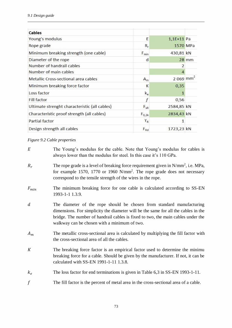
9.1 Design guide
73
Figure 9.2 Cable properties
𝐸 The Young’s modulus for the cable. Note that Young’s modulus for cables is
always lower than the modulus for steel. In this case it’s 110 GPa.
𝑅𝑟 The rope grade is a level of breaking force requirement given in N/mm2, i.e. MPa,
for example 1570, 1770 or 1960 N/mm2. The rope grade does not necessary
correspond to the tensile strength of the wires in the rope.
𝐹𝑚𝑖𝑛 The minimum breaking force for one cable is calculated according to SS-EN
1993-1-1 1.3.9.
𝑑 The diameter of the rope should be chosen from standard manufacturing
dimensions. For simplicity the diameter will be the same for all the cables in the
bridge. The number of handrail cables is fixed to two, the main cables under the
walkway can be chosen with a minimum of two.
𝐴𝑚 The metallic cross-sectional area is calculated by multiplying the fill factor with
the cross-sectional area of all the cables.
𝐾 The breaking force factor is an empirical factor used to determine the minimu
breaking force for a cable. Should be given by the manufacturer. If not, it can be
calculated with SS-EN 1991-1-11 1.3.8.
𝑘𝑒 The loss factor for end terminations is given in Table 6,3 in SS-EN 1993-1-11.
𝑓 The fill factor is the percent of metal area in the cross-sectional area of a cable.

9.1 Design guide
74
𝐹𝑢𝑘 The characteristic value of breaking strength is calculated according to equation
6,4 in SS-EN 1993-1-11.
𝐹0,2𝑘 The characteristic proof strength is the maximum strength of the cable without
exceeding a permanent strain of 0,2 %.
𝛾𝑅 The partial factor used in equation 6,2 in SS-EN 1993-1-11.
𝐹𝑅𝑑 The total design strength for all cables is calculated with equation 6,2 in SS-EN
1993-1-11. The equation can be seen below:
𝐹𝑅𝑑 = 𝑚𝑖𝑛 {𝐹𝑢𝑘
1,5 ∙ 𝛾𝑅;𝐹𝑘
𝛾𝑅
} (9.1)
In Figure 9.3 below, the loads acting on the bridge can be seen. These loads are the same as the
loads presented in chapter 2.10.3. The only load that has to be given is the horizontal wind load
for the current bridge. The other loads, both dead load and live load, will be calculated
automatically. The load combination creating the worst load situation will be the design load.
In almost all cases, load combination 6,10b will be the design load combination.
In this sheet, the windguys are assumed to carry all the horizontal wind load. In the sheet for
spans under 120 meter, an enlargement factor will be added to the vertical loads to compensate
for the displacement caused by the wind load, as described in chapter 2.10.5. This enlargement
factor will be calculated and added automatically.
Figure 9.3 Loads
When the loads and load combinations are determined the hoisting sag and the full load sag
can be determined. This is done in an iterative way for both the hoisting sag and the full load
sag. The numbers of iterations varies depending on the loads.

9.1 Design guide
75
Figure 9.4 Hoisting sag iteration procedure
𝐿 The cable length is the total length of the cable.
𝐶 The constant factor gather all the constants in the iteration procedure. The formula
used can be seen in Figure 9.4.
𝑏ℎ∗
𝑠𝑡𝑎𝑟𝑡 The primary hoisting sag is the starting value for the hoisting sag in the iteration
procedure. The starting value is set to 93 % of the dead load sag.
𝑔∗ The primary hoisting load is the load used for calculating the primary hoisting sag
in every iteration. Will with every iteration move closer to the real hoisting load.
𝑏ℎ∗ The primary hoisting sag is the sag determined with the primary hoisting load in
the current iteration.
∆𝑔𝑖 The load difference is the difference between the primary hoisting load and the
real hoisting load, i.e. ∆𝑔𝑖 = 𝑔ℎ − 𝑔∗. The condition to be fulfilled is that |∆𝑔𝑖| ≤
0,01 𝑘𝑁/𝑚. If this condition is fulfilled, the cell to the right will sign OK.
𝑏ℎ The final hoisting sag is set to the 𝑏ℎ∗ in the first iteration that fulfills the condition
|∆𝑔𝑖| ≤ 0,01 𝑘𝑁/𝑚. For example, in Figure 9.4 above, the 4th iteration fulfilled
the condition and 𝑏ℎ is therefore set to 6,11 meter.
When the hoisting sag has been determined, the same procedure is followed to determine the
full load sag. The same unit are used as in the hoisting sag procedure. The only difference is
that the prefixes are changed from ℎ to 𝑑, which can be seen in FIGURE XXX

9.1 Design guide
76
Figure 9.5 Full load sag iteration procedure
As it can be seen in Figure 9.5, the maximum tension in the cables due to the full load, is
calculated with the full load sag. In the figure above, the full load sag is determined to be 9,2
meter and the tension in the cables 1,67 MN. In the bottom of the figure is the structural capacity
for the cables checked against the maximum tension. If the capacity is greater than the
maximum tension in the cables, the safety factor, i.e. the capacity divided by the maximum
tension, is larger than 1. If this condition is fulfilled, the cell to the right will sign “OK”. If the
condition isn’t fulfilled, it will sign “Not OK”. When this condition is fulfilled, the design of
the load carrying cables of the bridge is done.
Windguys
Designing the windguys is a more complicated task. Four different anchors have to be installed.
Hopefully, the ground conditions are favorable so a symmetric position of the anchors is
possible. Otherwise a more detailed design procedure have to be done.
But let’s assume favorable ground conditions and a bridge with no height difference between
its saddles. This means that the windguys will be symmetric and that it’s enough to design only
one of the windguys. This has been assumed in the design guide, and otherwise the Helvetas
Long San Trail Bridge Standard should be used. Note that the design guide contains many
pictures explaining the geometric properties of the windguys. These picture has not been
included in this document due to publicity rights. The figure below contains the geometric
properties, the wind load and the resulting tension in the windguy cable/cables.

9.1 Design guide
77
Figure 9.6 Windguy geometry
Note that when the term in-plane is used here it mean as viewed in plan.
𝑙 The design span is the horizontal distance between the two saddles.
𝑣𝑅 The horizontal distance from the right abutment to the in-plane vertex for the
windguy cable. For a bridge with abutments at the same height, 𝑣𝑅 has the same
value as 𝑒 for the bridge.
𝑓𝑤 The in-plane sag of the windguy cable measured from the right abutment of the
bridge.
𝐻1 Elevation of the highest bridge abutment. In this case the elevation is the same for
both the abutments.
𝐻𝑅 Elevation of the right windguy foundation.
𝐻𝐿 Elevation of the left windguy foundation.
ℎ𝑤 The horizontal in-plane distance between the crossing points between the
windguy cable and the abutments, i.e. the in-plane distance from the windguy
cable to the bridge axis at the left abutment minus the same distance at the right
abutment. For a symmetric windguy, this distance is zero.

9.1 Design guide
78
𝑏𝑤 The in-plane sag of the windguy cable at midspan. If ℎ𝑤 = 0, i.e. a symmetric
windguy, 𝑏𝑤 = 𝑓𝑤 .
𝑑 The distance between the windties, i.e. the cables connection the windguy to the
bridge. 𝑑 should be equal to 6 meter for suspended bridges.
𝑘 The distance from the midpoint of the crossbeam to the connection with the
windtie.
𝑤 The wind load, which is determined in the earlier parts of the design guide.
𝐻𝑤 The horizontal force in the windguy cable
𝑇𝑅 The force in the windguy cable at the right foundation
𝑇𝐿 The force in the windguy cable at the left foundation
𝑇𝑤,𝑚𝑎𝑥 The largest of 𝑇𝑅 and 𝑇𝐿.
In the figure below, the cables are designed in the same way as in the earlier part. The only
difference is that one have to choose the number of cable in each windguy, 𝑛𝑤, which most
often is one or two. For example,in the figure below it was enough with one.
Figure 9.7 Windguy porperties

9.1 Design guide
79
𝐵𝑅 The horizontal distance from the right abutment to the first windtie.
𝐵𝐿 The horizontal distance from the left abutment to the first windtie.
𝛼𝑅 The in-plane inclination between the windguy and the bridge axis at the right
abutment.
𝛼𝐿 The in-plane inclination between the windguy and the bridge axis at the left
abutment.
𝐶𝑅 The in-plane, orthogonal to the bridge axis, distance between the right bridge
abutment and the right windguy foundation.
𝐶𝐿 The in-plane, orthogonal to the bridge axis, distance between the left bridge
abutment and the left windguy foundation.
𝐶𝑅𝑜 The in-plane, orthogonal to the bridge axis, distance between the right bridge
abutment and the windguy.
𝐶𝐿𝑜 The in-plane, orthogonal to the bridge axis, distance between the left bridge
abutment and the windguy.
𝐷𝑅 The in-plane, along the bridge axis, distance between the right bridge abutment
and the right windguy foundation. Negative if the windguy foundation is closer
than the abutment to the midpoint of the span.
𝐷𝐿 The in-plane, along the bridge axis, distance between the left bridge abutment and
the right windguy foundation. Negative if the windguy foundation is closer than
the abutment to the midpoint of the span.
𝐹 The safety factor is finally determined by dividing the structural capacity of the
windguy, 𝑓𝑅𝑑 with the maximum force 𝑇𝑤,𝑚𝑎𝑥. If the safety factor exceeds 1, the
design is correct.
Windties
The windties connects the bridge to the windguy. The length of the windties can be determined
with a series of parabolas that describes the shape of the bridge and the windguy in both plan
and elevation.

9.1 Design guide
80
Figure 9.8 Windties properties
𝛾 The inclination between the windtie at the walkway vertex and the horizontal
plane.
𝑦𝑙𝑝 The horizontal distance from the windguy to the wintie connecting bolt at the
vertex of the walkway.
∆ℎ𝑙𝑝 The vertical distance from the windguy to the wintie connecting bolt at the vertex
of the walkway.
𝑃𝑎𝑟𝑎𝑏𝑜𝑙𝑎 1 The parabola that describes the elevation of the suspended bridge.
𝑃𝑎𝑟𝑎𝑏𝑜𝑙𝑎 2 The parabola that describes the elevation of the windguy to the right side of the
walkway vertex.
𝑃𝑎𝑟𝑎𝑏𝑜𝑙𝑎 3 The parabola that describes the elevation of the windguy to the left side of the
walkway vertex.
𝑃𝑎𝑟𝑎𝑏𝑜𝑙𝑎 4 The parabola that describes the plan of the windguy.
The parabola equation used is:
𝑦 𝑜𝑟 𝑧 = 𝑎𝑖 ∙ 𝑥2 + 𝑐𝑖
where x is parallel to the bridge axis. The parabolas and the geometry can be seen in the design
guide.
Finally the length of the windties is determined.

9.1 Design guide
81
Figure 9.9 Length of windties
As it can be seen in the figure above, it’s important to use parabola 2 for values x>0 and parabola
for values x<0.
Finally, note that if a non-symmetric bridge is designed, formulas might need to be changed.
Please check the Long Span Trail Bridge Standard in this case.

9.2 Natural frequencies and appurtenant modes
82
9.2 Natural frequencies and appurtenant modes
Figure 9.10 Third out of plane mode shape for Jicaro Bridge
Figure 9.11 Second in-plane mode shape for Jicaro Bridge

9.2 Natural frequencies and appurtenant modes
83
Figure 9.12 Third in-plane mode shape for Jicaro Bridge
Figure 9.13 First out of plane mode shape for 150 m span bridge

9.2 Natural frequencies and appurtenant modes
84
Figure 9.14 Second out of plane mode shape for 150 m span bridge
Figure 9.15 Third out of plane mode shape for 150 m span bridge
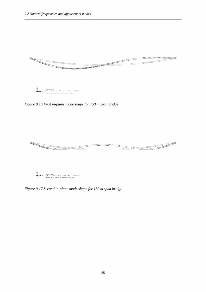
9.2 Natural frequencies and appurtenant modes
85
Figure 9.16 First in-plane mode shape for 150 m span bridge
Figure 9.17 Second in-plane mode shape for 150 m span bridge

9.2 Natural frequencies and appurtenant modes
86
Figure 9.18 Third in-plane mode shape 150 m span bridge
Figure 9.19 First out of plane mode shape 150 m span bridge with windguys

9.2 Natural frequencies and appurtenant modes
87
Figure 9.20 Second out of plane mode shape 150 m span bridge with windguys
Figure 9.21 Third out of plane mode shape 150 m span bridge with windguys

9.2 Natural frequencies and appurtenant modes
88
Figure 9.22 First in-plane mode shape 150 m span bridge with windguys
Figure 9.23 Second in-plane mode shape 150 m span bridge with windguys
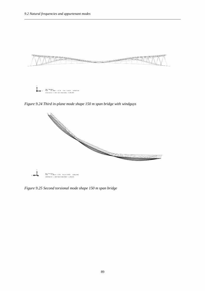
9.2 Natural frequencies and appurtenant modes
89
Figure 9.24 Third in-plane mode shape 150 m span bridge with windguys
Figure 9.25 Second torsional mode shape 150 m span bridge
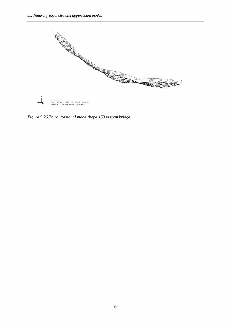
9.2 Natural frequencies and appurtenant modes
90
Figure 9.26 Third torsional mode shape 150 m span bridge