ANALYSIS OF SOME KRYLOV SUBSPACE APPROXIMATIONS

TO THE MATRIX EXPONENTIAL OPERATOR

Y. SAAD ∗

Abstract. In this note we present a theoretical analysis of some Krylov subspace approximationsto the matrix exponential operation exp(A)v and establish a priori and a posteriori error estimates.Several such approximations are considered. The main idea of these techniques is to approximatelyproject the exponential operator onto a small Krylov subspace and carry out the resulting smallexponential matrix computation accurately. This general approach, which has been used with successin several applications, provides a systematic way of defining high order explicit-type schemes forsolving systems of ordinary differential equations or time-dependent Partial Differential Equations.

1. Introduction. The problem of approximating the operation exp(A)v for agiven vector v and a matrix A is of considerable importance in many applications.For example, this basic operation is at the core of many methods for solving systems ofordinary differential equations (ODE’s) or time-dependent partial differential equations(PDE’s). Recently, the use of Krylov subspace techniques in this context has been ac-tively investigated in the literature [2, 3, 4, 9, 10]. Friesner et al. [2] and Gallopoulos andSaad [3] introduced a few different ways of applying this approximation to the solutionof systems of ordinary differential equations. The paper [3] presents some analysis onthe quality of the Krylov approximation and on the ODE integration schemes derivedfrom it. In this note we make the following contributions.

1. We introduce and justify a few new approximation schemes (Section 2);2. We analyze the Krylov subspace approach from an approximation theory view-

point. In particular we establish that the Krylov methods are equivalent tointerpolating the exponential function on the associated Ritz values (Section3);

3. We generalize some of the a priori error bounds proved in [3] (Section 4);4. Finally, we present a posteriori error bounds (Section 5) that are essential for

practical purposes.The basic idea of the Krylov subspace techniques considered in this paper is to

approximately project the exponential of the large matrix onto a small Krylov subspace.The only matrix exponential operation performed is therefore with a much smallermatrix. This technique has been successfully used in several applications, in spite ofthe lack of theory to justify it. For example, it is advocated in the paper by Park andLight [10] following the work by Nauts and Wyatt [7, 8]. Also, the idea of exploiting theLanczos algorithm to evaluate terms of the exponential of Hamiltonian operators seemsto have been first used in Chemical Physics, by Nauts and Wyatt [7]. The general Krylovsubspace approach for nonsymmetric matrices was used in [4] for solving parabolicequations, and more recently, Friesner et al. [2] demonstrated that this technique can

∗ University of Minnesota, Computer Science department, EE/CS building, Minneapolis, MN 55455.Work supported by the NAS Systems Division and/or DARPA via Cooperative Agreement NCC 2-387between NASA and the University Space Research Association (USRA).

1

be extended to solving systems of stiff nonlinear differential equations. In the workby Nour-Omid [9] systems of ODEs are solved by first projecting them onto Krylovsubspaces and then solving reduced tridiagonal systems of ODEs. This is equivalentto the method used in [10] which consists of projecting the exponential operator onthe Krylov subspace. The evaluation of arbitrary functions of a matrix with Krylovsubspaces has also been briefly mentioned by van der Vorst [13].

The purpose of this paper is to explore these techniques a little further both from apractical and a theoretivcal viewpoint. On the practical side we introduce new schemesthat can be viewed as simple extensions or slight improvements of existing ones. We alsoprovide a-posteriori error estimates which can be of help when developing integrationschemes for ODE’s. On the theoretical side, we prove some characterization results anda few additional a priori error bounds.

2. Krylov subspace approximations for eAv . We are interested in approxi-mations to the matrix exponential operation exp(A)v of the form

eAv ≈ pm−1(A)v,(1)

where A is a matrix of dimension N , v an arbitrary nonzero vector, and pm−1 is apolynomial of degree m − 1. Since this approximation is an element of the Krylovsubspace

Km ≡ span{v, Av, . . . , Am−1v},

the problem can be reformulated as that of finding an element of Km that approximatesu = exp(A)v. In the next subsections we consider three different possibilities for findingsuch approximations. The first two are based on the usual Arnoldi and nonsymmetricLanczos algorithms respectively. Both reduce to the same technique when the matrixis symmetric. The third technique presented can be viewed as a corrected version ofeither of these two basic approaches.

2.1. Exponential propagation using the Arnoldi algorithm. In this sectionwe give a brief description of the method presented in [3] which is based on Arnoldi’s al-gorithm. The procedure starts by generating an orthogonal basis of the Krylov subspacewith the well-known Arnoldi algorithm using v1 = v/‖v‖2 as an initial vector.

Algorithm: Arnoldi

1. Initialize: Compute v1 = v/‖v‖2.2. Iterate: Do j = 1, 2, ...,m

(a) Compute w := Avj

(b) Do i = 1, 2, . . . , ji. Compute hi,j := (w, vi)ii. Compute w := w − hi,jvi

(c) Compute hj+1,j := ‖w‖2 and vj+1 := w/hj+1,j.

2

Note that step 2-(b) is nothing but a modified Gram-Schmidt process. The abovealgorithm produces an orthonormal basis Vm = [v1, v2, . . . , vm] of the Krylov subspaceKm. If we denote the m×m upper Hessenberg matrix consisting of the coefficients hij

computed from the algorithm by Hm, we have the relation

AVm = VmHm + hm+1,mvm+1eTm,(2)

from which we get Hm = V Tm AVm. Therefore Hm represents the projection of the linear

transformation A onto the subspace Km, with respect to the basis Vm. Based on this,the following approximation was introduced in [3]:

eAv ≈ βVmeHme1.(3)

Since V Tm (τA)Vm = τHm and the Krylov subspaces associated with A and τA are

identical we can also write

eτAv ≈ βVmeτHme1,(4)

for an arbitrary scalar τ . The practical evaluation of the vector exp(τHm)e1 is discussedin Section 2.4. Formula (4) approximates the action of the operator exp(τA) which issometimes referred to as the exponential propagation operator. It has been observedin several previous articles that even with relatively small values of m a remarkablyaccurate approximation can be obtained from (3); see for example [3, 2, 9].

2.2. Exponential propagation using the Lanczos algorithm. Another well-known algorithm for building a convenient basis of Km is the well-known Lanczos algo-rithm. The algorithms starts with two vectors v1 and w1 and generates a bi-orthogonalbasis of the subspaces Km(A, v1) and Km(AT , w1).

Algorithm: Lanczos

1. Start: Compute v1 = v/‖v‖2 and select w1 so that (v1, w1) = 1.2. Iterate: For j = 1, 2, . . . ,m do:

• αj := (Avj, wj)• vj+1 := Avj − αjvj − βjvj−1

• wj+1 := AT wj − αjwj − δjwj−1

• βj+1 :=√

|(vj+1, wj+1)| , δj+1 := βj+1.sign[(vj+1, wj+1)]• vj+1 := vj+1/δj+1

• wj+1 := wj+1/βj+1

If we set, as before, Vm = [v1, v2, ...., vm] and, similarly, Wm = [w1, w2, ...., wm] then

W TmVm = V T

m Wm = I ,(5)

where I is the identity matrix. Let us denote by Tm the tridiagonal matrix

Tm ≡ Tridiag[δi, αi, βi+1].3

An analogue of the relation (2) is

AVm = VmTm + δm+1vm+1eTm,(6)

and an approximation similar to the one based on Arnoldi’s method is given by

eAv ≈ βVmeTme1,(7)

in which as before β = ‖v‖2. The fact that Vm is no longer orthogonal may cause somenonnegligible numerical difficulties since the norm of Vm may, in some instances, bevery large.

What can be said of one of these algorithms can often also be said of the other.In order to unify the presentation we will sometimes refer to (3) in which we use thesame symbol Hm to represent either the Hessenberg matrix Hm in Arnoldi’s methodor the tridiagonal matrix Tm in the Lanczos algorithm. In summary, the features thatdistinguish the two approaches are the following:

• In the Arnoldi approximation Vm is orthogonal and Hm is upper Hessenberg;• In the Lanczos approximation Hm is tridiagonal and Vm is not necessarily

orthogonal;• In the symmetric case Vm is orthogonal and Hm is tridiagonal and symmetric.

2.3. Corrected schemes . In this section we will use the same unified notation(3) to refer to either the Arnoldi based approximation (3) or the Lanczos based ap-proximation (7). In the approximations described above, we generate m + 1 vectorsv1, ..., vm+1 but only the first m of them are needed to define the approximation. A nat-ural question is whether or not one can use the extra vector vm+1 to obtain a slightlyimproved approximation at minimal extra cost. The answer is yes and the alternativescheme which we propose is obtained by making use of the function

φ(z) =ez − 1

z.(8)

To approximate eAv we write

eAv = v + Aφ(A)v

and we approximate φ(A)v by

φ(A)v ≈ Vmφ(Hm)βe1.(9)

Denoting by sm the error sm ≡ φ(A)v1−Vmφ(Hm)e1 and making use of the relation (2)we then have

eAv1 = v1 + Aφ(A)v1

= v1 + A(Vmφ(Hm)e1 + sm)

= v1 + (VmHm + hm+1,mvm+1eTm)φ(Hm)e1 + Asm

= Vm[e1 + Hmφ(Hm)e1] + hm+1,meTmφ(Hm)e1vm+1 + Asm

= VmeHme1 + hm+1,meTmφ(Hm)e1vm+1 + Asm.(10)

4

The relation (10) suggests using the approximation

eAv ≈ β[

VmeHme1 + hm+1,meTmφ(Hm)e1 vm+1

]

(11)

which can be viewed as a corrected version of (3). As is indicated by the expression(10), the error in the new approximation is βAsm.

The next question we address concerns the practical implementation of these cor-rected schemes. The following proposition provides a straightforward solution.

Proposition 2.1. Define the (m + 1) × (m + 1) matrix

Hm ≡

(

Hm 0c 0

)

(12)

where c is any row vector of length m. Then,

eHm =

(

eHm 0cφ(Hm) 1

)

.(13)

The proof of the proposition is an easy exercise which relies on the Taylor seriesexpansion of the exponential function. Taking c = hm+1,meT

m, it becomes clear fromthe proposition and (11) that the corrected scheme is mathematically equivalent to theapproximation:

eAv ≈ βVm+1eHme1(14)

whose computational cost is very close to that of the original methods (3) or (7). Inthe remainder of the paper the matrix Hm is defined with c = hm+1,meT

m.Note that the approximation of φ(A)v is an important problem in its own right. It

can be useful when solving a system of ordinary differential equations w = −Aw + r,whose solution si given by w(t) = w0 + tφ(−tA)(r −Aw0). A transposed version of theabove proposition provides a means for computing vectors of the form φ(Hm)c whichcan be exploited for evaluating the right hand side of (9). In addition, the φ functionalso plays an important role in deriving a-posterior error estimates, see Section 5.

2.4. Use of rational functions. In this section we briefly discuss some aspectsrelated to the practical computation of exp(Hm)e1 or φ(Hm)e1. Additional details maybe found in [3]. Since m will, in general, be much smaller than N , the dimension of A, itis clear that any of the standard methods for computing exp(Hm)e1 may be acceptable.However, as was discussed in [3], for large m the cost may become nonnegligible ifan algorithm of order m3 is used especially when the computations are carried outon a supercomputer. In addition, the discussion in this section is essential for thedevelopment of the a posteriori error estimates described in Section 5.

Consider the problem of evaluating exp(H)b where H is a small, possibly dense,matrix. One way in which the exponential of a matrix is evaluated is by using rationalapproximation to the exponential function [3, 4]. Using a rational approximation R(z),

5

of the type (p, p), i.e., such that the denominator has the same degree p as the numerator,it is more viable and economical to use the partial fraction expansion of R, see [3],

R(z) = α0 +p

∑

i=1

αi

z − θi

,(15)

where the θi’s are the poles of R. Expressions for the αi’s and the θi’s for the Chebyshevapproximation to e−z on the positive real line are tabulated once and for all. Theapproximation to y = exp(H)b for some vector b can be evaluated via

y = α0b +p

∑

i=1

αi(H − θiI)−1b ,(16)

which normally requires p factorizations. In fact since the roots θi seem to come gen-erally in complex conjugate pairs we only need about half as many factorizations tobe carried out in complex arithmetic. The rational functions that are used in [3] aswell as in the numerical experiments section in this paper are based on the Chebyshevapproximation on [0,∞) of the function e−x, see [1] and the references therein. Thisapproximation is remarkably accurate and, in general, a small degree approximation, assmall as p = 14, suffices to obtain a good working accuracy. We also observe that theHessenberg or tridiagonal form are very desirable in this context: assuming the matrixH is of size m it costs O(pm2) to compute exp(H)e1 when H is Hessenberg and onlyO(pm) when it is tridiagonal. This is to be compared with a cost of O(m3) for a methodthat would compute exp(Hm) based on the Schur decomposition.

Concerning the computation of vectors of the form φ(A)b it is easily seen that ifthe rational approximation R(z) to ez is exact at z = 0, i.e., if R(0) = 1, then we canderive from the definition (8) the following rational approximation to φ(z):

Rφ(z) =p

∑

i=1

αi

θi(z − θi).(17)

As a result, the same tables for the coefficients αi and the roots θi can be used tocompute either exp(H)b or φ(H)b. This is exploited in Section 5.

3. Characterization and Exactness. Throughout this section we will refer tothe eigenvalues of the matrix Hm (resp. Tm) as the Ritz values 1. We will denote byσ(X) the spectrum of a given square matrix X.

There are two theoretical questions we would like to address. First, we would like toexamine the relation between the methods described earlier and the problem of approx-imating the exponential function. As will be seen, these methods are mathematicallyequivalent to interpolating the exponential function over the Ritz values. Second, wewould like to determine when the Krylov approximation (3) becomes exact.

1 This constitutes a slight abuse of the terminology since this term is generally used in the Hermitiancase only.

6

3.1. Characterization. The following lemma is fundamental in proving a numberof results in this paper.

Lemma 3.1. Let A be any matrix and Vm, Hm the results of m steps of the Arnoldior Lanczos method applied to A. Then for any polynomial pj of degree j ≤ m − 1 thefollowing equality holds

pj(A)v1 = Vmpj(Hm)e1(18)

Proof. Consider the Arnoldi case first. Let πm = VmV Tm be the orthogonal projector

onto Km as represented in the original basis. We will prove by induction that Ajv1 =VmHj

me1, for j = 0, 1, 2, ...,m − 1. The result is clearly true for j = 0. Assume that itis true for some j with j ≤ m− 2. Since the vectors Aj+1v1 and Ajv1 belong to Km wehave

Aj+1v1 = πmAj+1v1 = πmAAjv1 = πmAπmAjv1 .

The relation (2) yields πmAπm = VmHmV Tm . Using the induction hypothesis we get,

Aj+1v1 = VmHmV Tm VmHj

me1 = VmHj+1m e1.

This proves the result for the Arnoldi case. The proof for the Lanczos approximation(7) is identical except that πm must be replaced by the oblique projector VmW T

m.Let now qν be the minimal polynomial of an arbitrary matrix A, where ν is its

degree. We know that any power of the matrix A can be expressed in terms of apolynomial in A, of degree not exceeding ν − 1. An immediate consequence is that iff(z) is an entire function then f(A) = pν−1(A) for a certain polynomial of degree atmost ν − 1. The next lemma determines this polynomial. Recall that a polynomial pinterpolates a function f in the Hermite sense at a given point x repeated k times if f

and p as well as their k − 1 first derivatives agree at x.Lemma 3.2. Let A be any matrix whose minimal polynomial is of degree ν and

f(z) a function in the complex plane which is analytic in an open set containing thespectrum of A. Moreover, let pν−1 be the interpolating polynomial of the function f(z),in the Hermite sense, at the roots of the minimal polynomial of A, repeated accordingto their multiplicities. Then:

f(A) = pν−1(A) .(19)

See [5] for a proof.Consider now a Hessenberg matrix H. It is known that whenever hj+1,j 6= 0, j =

1, 2, ...,m − 1, the geometric multiplicity of each eigenvalue is one, i.e., the minimalpolynomial of H is simply its characteristic polynomial. Therefore, going back to theHessenberg matrix provided by the Arnoldi process, we can state that

eHm = pm−1(Hm).(20)

7

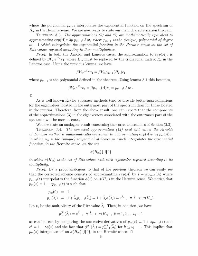
where the polynomial pm−1 interpolates the exponential function on the spectrum ofHm in the Hermite sense. We are now ready to state our main characterization theorem.

Theorem 3.3. The approximations (3) and (7) are mathematically equivalent toapproximating exp(A)v by pm−1(A)v, where pm−1 is the (unique) polynomial of degreem − 1 which interpolates the exponential function in the Hermite sense on the set ofRitz values repeated according to their multiplicities.

Proof. In both the Arnoldi and Lanczos cases, the approximation to exp(A)v isdefined by βVmeHme1, where Hm must be replaced by the tridiagonal matrix Tm in theLanczos case. Using the previous lemma, we have

βVmeHme1 = βVmpm−1(Hm)e1

where pm−1 is the polynomial defined in the theorem. Using lemma 3.1 this becomes,

βVmeHme1 = βpm−1(A)v1 = pm−1(A)v .

As is well-known Krylov subspace methods tend to provide better approximationsfor the eigenvalues located in the outermost part of the spectrum than for those locatedin the interior. Therefore, from the above result, one can expect that the componentsof the approximations (3) in the eigenvectors associated with the outermost part of thespectrum will be more accurate.

We now state an analogous result concerning the corrected schemes of Section (2.3).Theorem 3.4. The corrected approximation (14) used with either the Arnoldi

or Lanczos method is mathematically equivalent to approximating exp(A)v by pm(A)v,in which pm is the (unique) polynomial of degree m which interpolates the exponentialfunction, in the Hermite sense, on the set

σ(Hm)⋃

{0}

in which σ(Hm) is the set of Ritz values with each eigenvalue repeated according to itsmultiplicity.

Proof. By a proof analogous to that of the previous theorem we can easily seethat the corrected scheme consists of approximating exp(A) by I + Apm−1(A) wherepm−1(z) interpolates the function φ(z) on σ(Hm) in the Hermite sense. We notice thatpm(z) ≡ 1 + zpm−1(z) is such that

pm(0) = 1

pm(λi) = 1 + λipm−1(λi) = 1 + λiφ(λi) = eλi , ∀ λi ∈ σ(Hm).

Let νi be the multiplicity of the Ritz value λi. Then, in addition, we have

p(k)m (λi) = eλi , ∀ λi ∈ σ(Hm) , k = 1, 2, ..., νi − 1

as can be seen by comparing the successive derivatives of pm(z) ≡ 1 + zpm−1(z) and

ez = 1 + zφ(z) and the fact that φ(k)(λi) = p(k)m−1(λi) for k ≤ νi − 1. This implies that

pm(z) interpolates ez on σ(Hm)⋃

{0}, in the Hermite sense.8

The above result justifies the term “corrected schemes” used for the techniquesderived in Section 2.3, since these correspond to adding one additional constraint to theapproximations. They can therefore be expected to be slightly more accurate than theparent schemes while their costs are essentially identical.

3.2. Exactness. By analogy with conjugate gradient algorithms, we might wonderif the degree of the minimal polynomial of v with respect to A is also an upper boundon the dimension m needed to get the exact solution by the formula (3). As will beshown the answer is yes. In this section we consider only the Arnoldi based method ofSection 2.1.

Consider the case where at some step m we have hm+1,m = 0 in the Arnoldi process.In this situation, the algorithm stops. This is referred to as a ‘lucky breakdown’ because(2) simplifies into AVm = VmHm, which implies that Km is an invariant subspace.Moreover, it is clear that Km will be the first of the sequence of Krylov subspacesKi for which this happens; otherwise the algorithm would have stopped at an earlierstep. As a result of the above relation we will have AkVm = VmHk

m for all k and theTaylor series expansion of the exponential function shows that the approximation (3)is exact. Clearly, (4) is also exact for any τ in this situation. As is well-known, this‘lucky breakdown’ occurs if and only if the minimum degree of v is equal to m and wehave therefore proved the following result.

Proposition 3.5. When the minimal polynomial of v is of degree equal to m, theKrylov approximation (4) is exact for all τ . In particular, since the minimum degreeof v cannot exceed N , the algorithm will deliver the exact answer for m ≤ N . Theabove exactness condition is also sufficient, as is shown next.

Theorem 3.6. The following three conditions are equivalent:(i) eτAv = βVmeτHme1 , ∀τ ;(ii) The Krylov subspace Km is invariant under A, and no subspace Ki with i < m is

invariant;(iii) The minimal polynomial of v is of degree equal to m.

Proof. That (iii) is equivalent to (ii) is a simple and well-known result on Krylovsubspaces and was essentially proved above, see also [11]. In addition, the previousproposition shows that (ii) → (i).

It remains to show that (i) → (ii). Taking the derivative of order k (with respectto τ) of the condition in (i) we get,

AkeτAv = βVmHkmeτHme1 , ∀ τ.

In particular, taking τ = 0 leads to the relation

Akv = βVmHkme1 ,

which establishes that Akv is in Km for all k. This proves in particular that any vectorin AKm which is a linear combination of the vectors Akv, k = 1, . . . ,m is in Km. Asa result Km is invariant under A. Moreover, we cannot have a Ki invariant under Awith i<m; otherwise the dimension of Km would be less than m, which would be acontradiction since Vm is an orthogonal basis of Km.

9

We note that the characteristic properties shown in the previous section could alsohave been used to prove the above theorem.

4. General a priori error bounds. In this section we establish general a priorierror bounds for the approximations defined in Section 2. Related results have beenshown in [3] for the Arnoldi-based algorithm. Here we aim at showing general errorbounds for all the algorithms presented earlier. Some analysis on their optimality isalso provided.

4.1. Preliminary Lemmas. The following lemma shows how to systematicallyexploit polynomial approximations to ex, in order to establish a priori error bounds.They generalize a result shown in [3].

Lemma 4.1. Let A be an arbitrary matrix and Vm, Hm the results of m steps of theArnoldi or the Lanczos process. Let f(z) be any function such that f(A) and f(Hm)are defined. Let pm−1 be any polynomial of degree ≤ m − 1 approximating f(z), anddefine the remainder rm(z) ≡ ez − pm−1(z). Then,

f(A)v − βVmf(Hm)e1 = β [rm(A)v1 − Vmrm(Hm)e1](21)

Proof. As a result of the relation f(z) = pm−1(z) + rm(z) we have

f(A)v1 = pm−1(A)v1 + rm(A)v1.(22)

Lemma 3.1 implies that

pm−1(A)v1 = Vmpm−1(Hm)e1.(23)

Similarly to (22) we can write for Hm

pm−1(Hm)e1 = f(Hm)e1 − rm(Hm)e1.(24)

To complete the proof, we substitute (24) in (23) and the resulting equation in (22) toget, after multiplying through by β

f(A)v = βVmf(Hm)e1 + β[rm(A)v1 − Vmrm(Hm)e1].

Note that for Arnoldi’s method the orthogonality of Vm immediately yields

‖f(A)v − βVmf(Hm)e1‖2 ≤ β(‖rm(A)‖2 + ‖rm(Hm)‖2)(25)

whereas for the Lanczos process we can only say that

‖f(A)v − βVmf(Hm)e1‖2 ≤ β(‖rm(A)‖2 + ‖Vm‖2‖rm(Tm)‖2).(26)

The following lemma will be useful in proving the next results.

10

Lemma 4.2. Let sm−1 be the polynomial of degree m − 1 obtained from the partialTaylor series expansion of ex, i.e.,

sm−1(x) =m−1∑

j=0

xj

j!,

and let tm(x) = ex − sm−1(x) be the remainder. Then, for any nonnegative real numberx and any nonnegative integer m:

tm(x) =xm

m!(1 + o(1)) ≤

xmex

m!(27)

Proof. The integral form of the remainder in the Taylor series for ex is

tm(x) =xm

(m − 1)!

∫ 1

0e(1−τ)xτm−1dτ(28)

Following the argument in the proof of Theorem 1 in [12], we notice that as m increasesthe term inside the integrand becomes an increasingly narrow spike centered aroundτ = 1. As a result the function e(1−τ)x in that narrow interval can be assimilated to theconstant function whose value is one and we can write

∫ 1

0e(1−τ)xτm−1dτ = (1 + o(1))

∫ 1

0τm−1dτ =

1

m(1 + o(1))

which proves the first part of (27). The inequality in the right-hand-side of (27) isobtained by using the inequality e(1−τ)x ≤ ex in the integral (28).

4.2. A priori error bounds for the basic schemes. We will now prove thefollowing theorem.

Theorem 4.3. Let A be any matrix and let ρ = ‖A‖2. Then the error of theapproximation (3) obtained using Arnoldi’s method is such that

‖eAv − βVmeHme1‖2 ≤ 2βtm(ρ) ≤ 2βρmeρ

m!.(29)

Similarly, the error of the approximation (7) obtained using the Lanczos method is suchthat

‖eAv − βVmeTme1‖2 ≤ β[tm(ρ) + ‖Vm‖2tm(ρ)] ≤(

ρmeρ + ‖Vm‖2ρmeρ

)

(30)

in which ρ = ‖Tm‖2.Proof. The proof of the theorem makes use of the particular polynomial sm(z)

where sm is defined in Lemma 4.2. For this polynomial, we have,

‖rm(A)v1‖2 = ‖∞∑

j=m

1

j!Ajv1‖2 ≤

∞∑

j=m

1

j!‖Ajv1‖2 ≤

∞∑

j=m

ρj

j!= tm(ρ).(31)

11

We consider first the Arnoldi case. We can prove that similarly to (31) we have

‖rm(Hm)e1‖2 ≤ tm(ρ) ,(32)

where ρ = ‖Hm‖2 = ‖V Tm AVm‖2. Observing (e.g. from (28)) that tm is an increasing

function of x for x positive, and that ρ ≤ ρ, we obtain

tm(ρ) ≤ tm(ρ).(33)

Substituting (33), (32) and (31) in inequality (25) yields the first part of the result (29).The second part of (29) is a consequence of the inequality in Lemma 4.2.

For the Lanczos case, (32) becomes

‖rm(Tm)e1‖2 ≤ tm(ρ)

where ρ = ‖Tm‖2 = ‖W TmAVm‖2. Unfortunately, in this case we cannot relate ρ and ρ.

Moreover, the norm of Vm is no longer equal to one. The result (30) follows immediatelyfrom (26), (31) and the above inequality.

We would like now to briefly discuss an asymptotic analysis in an attempt to de-termine how sharp the result may be in general. First, for m large enough in the aboveproof, the norm ‖A‖2 can be replaced by the spectral radius of A. This is because ‖Aj‖2

is asymptotically equivalent to |λmax|j, where |λmax| is the spectral radius. Secondly,

as is indicated by Lemma 4.2, tm(ρ) is in fact of the order of ρm/m!. In reality, wetherefore have

‖Error‖2 ≤ 2β|λmax|

m

m!(1 + o(1))

Moreover, as is indicated in [12], the polynomial sm−1 will be (asymptotically) near thepolynomial that best approximates the exponential function on a circle centered at theorigin. Therefore, if the eigenvalues of A are distributed in a circle of radius |λmax| onecan expect the above inequality to be asymptotically optimal.

In fact we now address the case where the matrix A has a spectrum that is enclosedin a ball of center α located far away from the origin. In such a case, the polynomialused in the above proof is inappropriate, in that it is likely to be far from optimal, andthe following lemma provides a better polynomial. In the following D(α, ρ) denotes theclosed disk of the complex plane centered at α and with radius ρ.

Lemma 4.4. Let sm−1 be the polynomial defined in Lemma 4.2 and let for any realα,

cm−1,α(z) = eαsm−1(z − α).

Then

maxz∈D(α,ρ)

|ez − cm−1,α(z)| ≤ eαtm(ρ) ≤ρmeρ+α

m!.(34)

12

Proof. From Lemma 4.2 for any z with |z − α| ≤ ρ we have

|ez−α − sm−1(z − α)| ≤∞∑

j=m

ρj

j!= tm(ρ) ≤

ρmeρ

m!(35)

Multiplying both sides by eα yields (34).As an application, we can prove the following theorem.Theorem 4.5. Let A be any matrix and ρα = ‖A − αI‖2 where α is any real

scalar. Then the error of the approximation (3) satisfies

‖eAv − βVmeHme1‖2 ≤ 2βeαtm(ρα) ≤ 2βρm

α eρα+α

m!.(36)

Proof. The proof is identical with that of Theorem (4.3) except that it uses thepolynomial cm−1,α defined in the previous lemma.

Ideally, we would like to utilize the best α possible in order to minimize the right-hand side of the inequality (36). However, this seems to be a rather difficult minimiza-tion problem to solve. The important factor in the inequality of the theorem is theterm ρα, which may be made much smaller than ρ, the norm of A, by a proper choiceof α. As a result we can nearly minimize the right-hand side of (36) by minimizingρα with respect to α, since the term eρα is asymptotically unimportant. According to(36) and to the discussion prior to the theorem, we can say that in the case where theeigenvalues of A are distributed in a disk of center α, and radius r, the error will behaveasymptotically like eαrm/m!, and this is likely to be an asymptotically sharp result. Inpractice the interesting cases are those where the spectrum is contained in the left halfof the complex plane. An important particular case in some applications is when thematrix A is symmetric negative definite.

Corollary 4.6. Let A be a symmetric definite negative matrix and let ρ = ‖A‖2.Then the error of the approximation (3) satisfies

‖eAv − βVmeHme1‖2 ≤ βρm

m!2m−1.(37)

Proof. We apply the previous theorem with α = −‖A‖2/2 and use the fact that the2-norm of a Hermitian matrices is equal to its spectral radius. Since A is symmetricdefinite negative, we have that ρα = |ρ/2| = −α. The proof follows immediately from(36).

In [3] it was shown that the term eρ in the right-hand side of (29) can be replacedby the term max(1, eη) where η = max{λi(A + AT )/2)} is the ‘logarithmic norm’ of A.

4.3. A priori error bounds for the corrected schemes. The corrected schemesare based on approximations using polynomials of the form p(z) = 1 + zpm−1(z), i.e.,polynomials of degree m satisfying the constraint p(0) = 1. In this section we proveresults similar to those of the Section 4.2, for the Arnoldi-based corrected scheme. We

13

do not consider the Lanczos-based approximation for which similar results can also beproved.

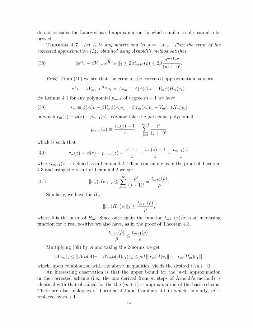
Theorem 4.7. Let A be any matrix and let ρ = ‖A‖2. Then the error of thecorrected approximation (14) obtained using Arnoldi’s method satisfies

‖eAv − βVm+1eHme1‖2 ≤ 2βtm+1(ρ) ≤ 2β

ρm+1eρ

(m + 1)!.(38)

Proof. From (10) we see that the error in the corrected approximation satisfies

eAv − βVm+1eHme1 = Asm ≡ A(φ(A)v − Vmφ(Hm)e1).

By Lemma 4.1 for any polynomial pm−1 of degree m − 1 we have

sm ≡ φ(A)v − βVmφ(A)e1 = β[rm(A)v1 − Vmrm(Hm)e1](39)

in which rm(z) ≡ φ(z) − pm−1(z). We now take the particular polynomial

pm−1(z) ≡sm(z) − 1

z=

m−1∑

j=1

zj

(j + 1)!

which is such that

rm(z) = φ(z) − pm−1(z) =ez − 1

z−

sm(z) − 1

z=

tm+1(z)

z(40)

where tm+1(z) is defined as in Lemma 4.2. Then, continuing as in the proof of Theorem4.3 and using the result of Lemma 4.2 we get

‖rm(A)v1‖2 ≤∞∑

j=m

ρj

(j + 1)!=

tm+1(ρ)

ρ.(41)

Similarly, we have for Hm

‖rm(Hm)e1‖2 ≤tm+1(ρ)

ρ,

where ρ is the norm of Hm. Since once again the function tm+1(x)/x is an increasingfunction for x real positive we also have, as in the proof of Theorem 4.3,

tm+1(ρ)

ρ≤

tm+1(ρ)

ρ.

Multiplying (39) by A and taking the 2-norms we get

‖Asm‖2 ≤ ‖A(φ(A)v − βVmφ(A)e1)‖2 ≤ ρβ [‖rm(A)v1‖ + ‖rm(Hm)e1‖] ,

which, upon combination with the above inequalities, yields the desired result.An interesting observation is that the upper bound for the m-th approximation

in the corrected scheme (i.e., the one derived from m steps of Arnoldi’s method) isidentical with that obtained for the the (m + 1)-st approximation of the basic scheme.There are also analogues of Theorem 4.2 and Corollary 4.1 in which, similarly, m isreplaced by m + 1.

14

5. A posteriori error estimates. The error bounds established in the previoussection may be computed, provided we can estimate the norm of A or A−αI. However,the fact that they may not be sharp leads us to seek alternatives. A posteriori errorestimates are crucial in practical computations. It is important to be able to assess thequality of the result obtained by one of the techniques described in this paper in orderto determine whether or not this result is acceptable. If the result is not acceptable thenone can still utilize the Krylov subspace computed to evaluate, for example, exp(Aδ)vwhere δ is chosen small enough to yield a desired error level. We would like to obtainerror estimates that are at the same time inexpensive to compute and sharp. Withoutloss of generality the results established in this section are often stated for the scaledvector v1 rather than for the original vector v.

5.1. Expansion of the error. We seek an expansion formula for the error interms of Akvm+1, k = 0, 1, ...,∞. To this end we need to define functions similar to theφ function used in earlier sections. We define by induction,

φ0(z) = ez

φk+1(z) =φk(z) − φk(0)

z, k ≥ 0

We note that φk+1(0) is defined by continuity. Thus, the function φ1 is identical withthe function φ used in Section 2. It is clear that these functions are well-defined andanalytic for all k. We can now prove the following theorem. Recall that we are using aunified notation: Hm may in fact mean Tm in the case where Lanczos is used insteadof the Arnoldi algorithm.

Theorem 5.1. The error produced by the Arnoldi or Lanczos approximation (3)satisfies the following expansion:

eAv1 − VmeHme1 = hm+1,m

∞∑

k=1

eTmφk(Hm)e1A

k−1vm+1 ,(42)

while the corrected version (14) satisfies,

eAv1 − Vm+1eHme1 = hm+1,m

∞∑

k=2

eTmφk(Hm)e1A

k−1vm+1 .(43)

Proof. The starting point is the relation (10)

eAv1 = VmeHme1 + hm+1,meTmφ(Hm)e1vm+1 + As1

m(44)

in which we now define, more generally,

sjm = φj(A)v1 − Vmφj(Hm)e1 .

Proceeding as for the development of the formula (10), we write

φ1(A)v1 = φ1(0)v1 + Aφ2(A)v1

15

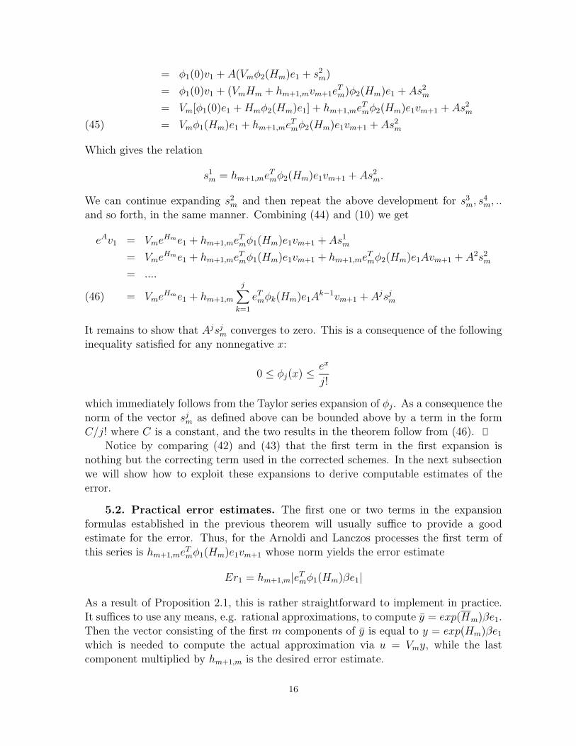
= φ1(0)v1 + A(Vmφ2(Hm)e1 + s2m)

= φ1(0)v1 + (VmHm + hm+1,mvm+1eTm)φ2(Hm)e1 + As2

m

= Vm[φ1(0)e1 + Hmφ2(Hm)e1] + hm+1,meTmφ2(Hm)e1vm+1 + As2

m

= Vmφ1(Hm)e1 + hm+1,meTmφ2(Hm)e1vm+1 + As2

m(45)

Which gives the relation

s1m = hm+1,meT

mφ2(Hm)e1vm+1 + As2m.

We can continue expanding s2m and then repeat the above development for s3

m, s4m, ..

and so forth, in the same manner. Combining (44) and (10) we get

eAv1 = VmeHme1 + hm+1,meTmφ1(Hm)e1vm+1 + As1

m

= VmeHme1 + hm+1,meTmφ1(Hm)e1vm+1 + hm+1,meT

mφ2(Hm)e1Avm+1 + A2s2m

= ....

= VmeHme1 + hm+1,m

j∑

k=1

eTmφk(Hm)e1A

k−1vm+1 + Ajsjm(46)

It remains to show that Ajsjm converges to zero. This is a consequence of the following

inequality satisfied for any nonnegative x:

0 ≤ φj(x) ≤ex

j!

which immediately follows from the Taylor series expansion of φj. As a consequence thenorm of the vector sj

m as defined above can be bounded above by a term in the formC/j! where C is a constant, and the two results in the theorem follow from (46).

Notice by comparing (42) and (43) that the first term in the first expansion isnothing but the correcting term used in the corrected schemes. In the next subsectionwe will show how to exploit these expansions to derive computable estimates of theerror.

5.2. Practical error estimates. The first one or two terms in the expansionformulas established in the previous theorem will usually suffice to provide a goodestimate for the error. Thus, for the Arnoldi and Lanczos processes the first term ofthis series is hm+1,meT

mφ1(Hm)e1vm+1 whose norm yields the error estimate

Er1 = hm+1,m|eTmφ1(Hm)βe1|

As a result of Proposition 2.1, this is rather straightforward to implement in practice.It suffices to use any means, e.g. rational approximations, to compute y = exp(Hm)βe1.Then the vector consisting of the first m components of y is equal to y = exp(Hm)βe1

which is needed to compute the actual approximation via u = Vmy, while the lastcomponent multiplied by hm+1,m is the desired error estimate.

16

If a rough estimate of the error is desired, one may avoid invoking the φ1 functionby replacing φ1(Hm) by exp(Hm) leading to the estimate

Er2 = hm+1,m|eTmym|.

The above expression is reminiscent of a formula used to compute the residual norm oflinear systems solved by the Arnoldi or the Lanczos/ Bi-Conjugate Gradient algorithms.

For the corrected schemes a straightforward analogue of Er2 is

Er3 = hm+1,m|eTmφ1(Hm)βe1|.

We can also use the first term in the expansion (43) to get the more elaborate errorestimate for the corrected schemes:

Er4 = hm+1,m|eTmφ2(Hm)βe1|‖Avm+1‖2.

The above formula requires the evaluation of the norm of Avm+1. Although this iscertainly not a high price to pay there is one compelling reason why one would liketo avoid it: if we were to perform one additional matrix-vector product then whynot compute the next approximation which belongs the Krylov subspace Km+2? Wewould then come back to the same problem of seeking an error estimate for this newapproximation. Since we are only interested in an estimate of the error, it may besufficient to approximate Avm+1 using some norm estimate of A provided by the Arnoldiprocess. One possibility is to resort to the scaled Frobenius norm of Hm:

‖Avm+1‖2 ≈ ‖Hm‖F ≡

1

m

m∑

j=1

j+1∑

i=1

h2i,j

1/2

which yields

Er5 = hm+1,m|eTmφ2(Hm)βe1|‖Hm‖F .

There remains the issue of computing eTmφ2(Hm)(βe1) for Er4 and Er5. One

might use a separate calculation. However, when rational approximations are usedto evaluate exp(Hm)(βe1), a more attractive alternative exists. Assume that the vectory = exp(Hm)(βe1) is computed from the partial fraction expansion

y =p

∑

i=1

αi(Hm − θiI)−1(βe1).(47)

A consequence of Proposition 2.1 is that the last component of the result is eTmφ1(Hm)(βe1)

but we need eTmφ2(Hm)(βe1). Now observe that if instead of the coefficients αi we were

to use the coefficients αi/θi in (47) then, according to the formula (17) in Section 2.4,we would have calculated the vector φ1(Hm)(βe1) and the last component would bethe desired eT

mφ2(Hm)(βe1). This suggests that all we have to do is to accumulate thescalars

p∑

i=1

αi

θi

eTm+1(Hm − θiI)−1e1,(48)

17

a combination of the last components of the consecutive solutions of (47), as thesesystems are solved one after the other. The rest of the computation is in no waydisturbed since we only accumulate these components once the solution of each linearsystem is completed. Notice that once more the cost of this error estimator is negligible.We also point out that with this strategy there is no difficulty in getting more accurateestimates of the error which correspond to using more terms in the expansion (43). Forexample, it suffices to replace αi/θi in (48) by αi/θ

2i to get eT

mφ3(Hm)e1, and thereforea similar technique of accumulation can be used to compute the higher order terms inthe expansion.

These error estimates have been compared on a few examples described in Section 6.

5.3. Error with respect to the rational approximation. The vector eHme1

in (3) may be evaluated with the help of a rational approximation to the exponentialof the form (15), i.e., the actual approximation used is of the form

eAv1 ≈ VmR(Hm)e1(49)

In the symmetric case, the Chebyshev rational approximation to the exponential yields aknown error with respect to the exact exponential, i.e., using the same rational functionR,

‖eAv1 − R(A)v1‖2 = ηp

is known a priori from results in approximation theory. As a result one may be ableto estimate the total error by simply estimating the norm of the difference R(A)v1 −VmR(Hm)e1.

Proposition 5.2. The following is an exact expression of the error made whenR(A)v1 is approximated by VmR(Hm)e1.

R(A)v1 − VmR(Hm)e1 =p

∑

i=1

αiεi(A − θiI)−1vm+1(50)

in which

εi = −hm+1,meTm(Hm − θiI)−1e1.

Proof. We have

R(A)v1 − VmR(Hm)e1 = α0(v1 − Vme1) +p

∑

i=1

αi

[

(A − θiI)−1v1 − Vm(Hm − θiI)−1e1

]

=p

∑

i=1

αi(A − θiI)−1[v1 − (A − θiI)Vm(Hm − θiI)−1e1](51)

Using once more the relation (2) we have

v1 − (A − θiI)Vm(Hm − θiI)−1e1 = −hm+1,meTm(Hm − θiI)−1e1vm+1

18

Table 1

Actual error and estimates for basic method on example 1.

m Actual Err Er1 Er2

3 0.301D-01 0.340D-01 0.889D-015 0.937D-04 0.102D-03 0.466D-036 0.388D-05 0.416D-05 0.232D-047 0.137D-06 0.146D-06 0.958D-068 0.424D-08 0.449D-08 0.339D-079 0.119D-09 0.123D-09 0.105D-0810 0.220D-10 0.301D-11 0.287D-10

Table 2

Actual error and estimates for the corrected method on example 1.

m Actual Err Er4 Er5 Er3

3 0.484D-02 0.571D-02 0.599D-02 0.340D-015 0.992D-05 0.112D-04 0.115D-04 0.102D-036 0.351D-06 0.389D-06 0.399D-06 0.416D-057 0.108D-07 0.119D-07 0.121D-07 0.146D-068 0.298D-09 0.323D-09 0.329D-09 0.449D-089 0.230D-10 0.788D-11 0.803D-11 0.123D-0910 0.218D-10 0.174D-12 0.176D-12 0.301D-11

With the definition of εi the result follows immediately.Note that |εi| represents the residual norm for the linear system (A − θiI)x =

v1 when the approximation Vm(Hm − θiI)−1e1 is used for the solution, while εi(A −θiI)−1vm+1 is the corresponding error vector. Thus, an interpretation of the result ofthe proposition, is that the error R(A)v1 −VmR(Hm)e1 is equal to a linear combinationwith the coefficients αi, i = 1, ..., p of the errors made when the solution of each linearsystem (A − θI)x = v1 is approximated by Vm(Hm − θI)−1e1. These errors may beestimated by standard techniques in several different ways. In particular the conditionnumber of each matrix (A−θiI) can be estimated from the eigenvalues/ singular valuesof the Hessenberg matrix Hm − θiI.

6. Numerical experiments. The purpose of this section is to illustrate with thehelp of two simple examples how the error estimates provided in the previous sectionbehave in practice. In the first example we consider a diagonal matrix of size N = 100whose diagonal entries λi = (i + 1)/(N + 1), are uniformly distributed in the interval[0, 1]. In the second example the matrix is block diagonal with 2 x 2 blocks of the form

(

ai c−c ai

)

in which c = 12

and aj = (2 j − 1)/(N + 1) for j = 1, 2, ..., N/2. In the first examplethe vector v was selected so that the result u = exp(A)w is known to be the vector

19

Table 3

Actual error and estimates for basic method on example 2.

m Actual Err Er1 Er2

3 0.114D+00 0.128D+00 0.337D+005 0.164D-02 0.178D-02 0.816D-026 0.124D-03 0.134D-03 0.744D-037 0.107D-04 0.114D-04 0.751D-048 0.593D-06 0.627D-06 0.473D-059 0.399D-07 0.419D-07 0.358D-0610 0.181D-08 0.189D-08 0.180D-0711 0.105D-09 0.102D-09 0.109D-0812 0.346D-10 0.351D-11 0.425D-10

(1, 1, 1..., 1)T . In the second example it was generated randomly.To compute the coefficient vector ym we used the rational approximation outlined

in Section 2.4. Moreover, for the corrected schemes we used the same rational approxi-mations and the a posteriori errors have been calculated following the ideas at the endof Section 5.2. The rational function used in all cases is the Chebyshev approximationto ex of degree (14,14) on the real negative line [3].

Table 1 shows the results for example 1 using the Arnoldi method which in thiscase amounts to the usual symmetric Lanczos algorithm. The estimates are based onthe formulas Er2 and Er1 of Section 5.2. Using the corrected version of the Arnoldi al-gorithm we get the results in Table 2. Tables 3 and 4 show similar results for example 2.Note that as expected the columns Er1 and Er3 are identical.

We can make the following observations. First, the estimate Er1 is far more accu-rate than the estimate Er2 for the basic Arnoldi-Lanczos methods. However, we startseeing some difficulties for large values of m. These are due to the fact that the ratio-nal approximation does not yield an accurate enough answer for exp(Hm)e1. In factfor larger values of m the actual error stalls at the level 2.3 10−11 while the estimatescontinue to decrease sharply. Unfortunately, we did not compute the coefficients of therational approximation, as described in Section 2, beyond the degree (14, 14) used here.In fact one can speculate that the estimated errors in the tables should be close to theactual error that we would have obtained had we used more accurate rational approxi-mations. Second, the estimates Er1 and Er5 based on just one term of the expansionof the error shown in Theorem 5.1, are surprisingly sharp in these examples. Finally,note that, as expected from the theory, the corrected approximations are slightly moreaccurate than the basic approximations. The tables indicate that, roughly speaking,for the larger values of m we gain one step for free. Note also that for these examplesthe scaled Frobenius norm seems to give a rather good estimate of the norm ‖Avm+1‖2

as is revealed by comparing the values of Er4 and Er5.

7. Conclusion. The general analysis proposed in this paper shows that the tech-nique based on Krylov subspaces can provide an effective tool for approximating the

20

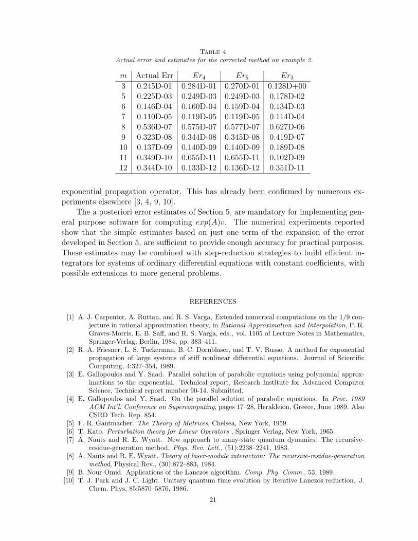
Table 4

Actual error and estimates for the corrected method on example 2.

m Actual Err Er4 Er5 Er3

3 0.245D-01 0.284D-01 0.270D-01 0.128D+005 0.225D-03 0.249D-03 0.249D-03 0.178D-026 0.146D-04 0.160D-04 0.159D-04 0.134D-037 0.110D-05 0.119D-05 0.119D-05 0.114D-048 0.536D-07 0.575D-07 0.577D-07 0.627D-069 0.323D-08 0.344D-08 0.345D-08 0.419D-0710 0.137D-09 0.140D-09 0.140D-09 0.189D-0811 0.349D-10 0.655D-11 0.655D-11 0.102D-0912 0.344D-10 0.133D-12 0.136D-12 0.351D-11

exponential propagation operator. This has already been confirmed by numerous ex-periments elsewhere [3, 4, 9, 10].

The a posteriori error estimates of Section 5, are mandatory for implementing gen-eral purpose software for computing exp(A)v. The numerical experiments reportedshow that the simple estimates based on just one term of the expansion of the errordeveloped in Section 5, are sufficient to provide enough accuracy for practical purposes.These estimates may be combined with step-reduction strategies to build efficient in-tegrators for systems of ordinary differential equations with constant coefficients, withpossible extensions to more general problems.

REFERENCES

[1] A. J. Carpenter, A. Ruttan, and R. S. Varga, Extended numerical computations on the 1/9 con-jecture in rational approximation theory, in Rational Approximation and Interpolation, P. R.Graves-Morris, E. B. Saff, and R. S. Varga, eds., vol. 1105 of Lecture Notes in Mathematics,Springer-Verlag, Berlin, 1984, pp. 383–411.

[2] R. A. Friesner, L. S. Tuckerman, B. C. Dornblaser, and T. V. Russo. A method for exponentialpropagation of large systems of stiff nonlinear differential equations. Journal of ScientificComputing, 4:327–354, 1989.

[3] E. Gallopoulos and Y. Saad. Parallel solution of parabolic equations using polynomial approx-imations to the exponential. Technical report, Research Institute for Advanced ComputerScience, Technical report number 90-14. Submitted.

[4] E. Gallopoulos and Y. Saad. On the parallel solution of parabolic equations. In Proc. 1989

ACM Int’l. Conference on Supercomputing, pages 17–28, Herakleion, Greece, June 1989. AlsoCSRD Tech. Rep. 854.

[5] F. R. Gantmacher. The Theory of Matrices, Chelsea, New York, 1959.[6] T. Kato. Perturbation theory for Linear Operators , Springer Verlag, New York, 1965.[7] A. Nauts and R. E. Wyatt. New approach to many-state quantum dynamics: The recursive-

residue-generation method, Phys. Rev. Lett., (51):2238–2241, 1983.[8] A. Nauts and R. E. Wyatt. Theory of laser-module interaction: The recursive-residue-generation

method, Physical Rev., (30):872–883, 1984.[9] B. Nour-Omid. Applications of the Lanczos algorithm. Comp. Phy. Comm., 53, 1989.

[10] T. J. Park and J. C. Light. Unitary quantum time evolution by iterative Lanczos reduction. J.Chem. Phys. 85:5870–5876, 1986.

21

[11] Y. Saad and M. H. Schultz. GMRES: a generalized minimal residual algorithm for solvingnonsymmetric linear systems. SIAM J. Sci. Statist. Comput, 7:856–869, 1986.

[12] L. N. Trefethen. The asymptotic accuracy of rational best approximation to ez in a disk. J.

Approx. Theory, 40:380-383, 1984.[13] H. van der Vorst. An iterative solution method for solving f(A) = b using Krylov subspace

information obtained for the symmetric positive definite matrix A. J. Comput. Appl. Math.,18:249–263, 1987.

22