analysis of singapore's foreign exchange market … the microstructure approach to exchange...
TRANSCRIPT

Singapore Management University
Institutional Knowledge at Singapore Management University
Analysis of Singapore's Foreign Exchange MarketMicrostructureChee Wai Wan

ANALYSIS OF SINGAPORE’S FOREIGN EXCHANGE
MARKET MICROSTRUCTURE
WAN CHEE WAI
SINGAPORE MANAGEMENT UNIVERSITY 2011

Copyright (2011) Wan Chee Wai
Analysis of
Singapore’s Foreign Exchange
Market Microstructure
by
Wan Chee Wai
Submitted to the School of Economics in partial fulfillment of the requirements for the Degree of Master of Science in Economics
Thesis Committee:
Tse Yiu Kuen (Supervisor/Chair) Professor of Economics Singapore Management University
Hoon Hian Teck Professor of Economics Singapore Management University Anthony Tay Associate Professor of Economics Singapore Management University
Singapore Management University 2011

Analysis of
Singapore’s Foreign Exchange
Market Microstructure
Wan Chee Wai
Abstract
This paper analyses the Singapore foreign exchange market from a
microstructure approach. Specifically, by applying and modifying the empirical
methodology designed by Bollerslev and Melvin (1994), we examine the
relationship between bid-ask spreads and the underlying volatility of the
USD/SGD. Our data set comprises high-frequency USD/SGD tick data of three
separate years (April-June 1989, April-May 2006, April-May 2009). We found
that for the USD/SGD: i) the size of bid-ask spreads are positively related to the
underlying exchange rate volatility; ii) the magnitude of the dependence on
underlying volatility increases as tick volume increases; and iii) the size of the
bid-ask spreads may also be positively related to the directional movement of
exchange rates.

i
Table of Contents
Table of Contents ......................................................................................................i
Acknowledgement ..................................................................................................iv
1 Introduction.......................................................................................................1
1.1 The Singapore Foreign Exchange Market ........................................................................2 1.2 The Microstructure Approach to Exchange Rate Economics ...........................................5 1.3 Organization of Thesis......................................................................................................9
2 Bid-Ask Spreads in Exchange Rates...............................................................10
2.1 Bid-Ask Spreads and Asymmetric Information.............................................................. 11 2.2 Bid-Ask Spreads and Volatility.......................................................................................18 2.3 Bollerslev & Melvin’s Model of Volatility and Bid-Ask Spread ....................................21
3 Empirical Analysis ..........................................................................................27
3.1 Empirical Methodology ..................................................................................................28 3.2 Description of the Data...................................................................................................34 3.3 GARCH Analysis ...........................................................................................................44 3.4 Ordered Response Analysis ............................................................................................47 3.5 Incorporating Returns .....................................................................................................50 3.6 Summary.........................................................................................................................53
4 Conclusion ......................................................................................................55
References..............................................................................................................57
Appendix 1 – EViews Results................................................................................60
A.1.1 Dataset 1: USD-DEM April 1989 to June 1989: ........................................................60 A.1.1.1 MA(1)-GARCH(1,1) Results: ....................................................................................60 A.1.1.2 Ordered Probit Results: 4 Ordered Values..................................................................61 A.1.1.3 Ordered Probit (with Returns) Results: 4 Ordered Values..........................................62 A.1.1.4 Ordered Probit Results: 10 Ordered Values................................................................63 A.1.1.5 Ordered Probit (with Returns) Results: 10 Ordered Values........................................64 A.1.1.6 Ordered Logit Results: 4 Ordered Values ...................................................................65 A.1.1.7 Ordered Logit (with Returns) Results: 4 Ordered Values ...........................................66 A.1.1.8 Ordered Logit Results: 10 Ordered Values .................................................................67 A.1.1.9 Ordered Logit (with Returns) Results: 10 Ordered Values .........................................68 A.1.2 Dataset 2: USD-USD April 1989 to June 1989: .........................................................69 A.1.2.1 MA(1)-GARCH(1,1) Results: ....................................................................................69 A.1.2.2 Ordered Probit Results: 4 Ordered Values..................................................................70 A.1.2.3 Ordered Probit (with Returns) Results: 4 Ordered Values..........................................71 A.1.2.4 Ordered Probit Results: 10 Ordered Values................................................................72 A.1.2.5 Ordered Probit (with Returns) Results: 10 Ordered Values........................................73 A.1.2.6 Ordered Logit Results: 4 Ordered Values ...................................................................74 A.1.2.7 Ordered Logit (with Returns) Results: 4 Ordered Values ...........................................75
ii
A.1.2.8 Ordered Logit Results: 10 Ordered Values .................................................................76 A.1.2.9 Ordered Logit (with Returns) Results: 10 Ordered Values .........................................77 A.1.3 Dataset 3: USD-USD April 2006 to May 2006: .........................................................78 A.1.3.1 MA(1)-GARCH(1,1) Results: ....................................................................................78 A.1.3.2 Ordered Probit Results: 4 Ordered Values..................................................................79 A.1.3.3 Ordered Probit (with Returns) Results: 4 Ordered Values..........................................80 A.1.3.4 Ordered Probit Results: 10 Ordered Values................................................................81 A.1.3.5 Ordered Probit (with Returns) Results: 10 Ordered Values........................................82 A.1.3.6 Ordered Logit Results: 4 Ordered Values ...................................................................83 A.1.3.7 Ordered Logit (with Returns) Results: 4 Ordered Values ...........................................84 A.1.3.8 Ordered Logit Results: 10 Ordered Values .................................................................85 A.1.3.9 Ordered Logit (with Returns) Results: 10 Ordered Values .........................................86 A.1.4 Dataset 4: USD-USD April 2009 to May 2009: .........................................................87 A.1.4.1 MA(1)-GARCH(1,1) Results: ....................................................................................87 A.1.4.2 Ordered Probit Results: 4 Ordered Values..................................................................88 A.1.4.3 Ordered Probit (with Returns) Results: 4 Ordered Values..........................................89 A.1.4.4 Ordered Probit Results: 10 Ordered Values................................................................90 A.1.4.5 Ordered Probit (with Returns) Results: 10 Ordered Values........................................91 A.1.4.6 Ordered Logit Results: 4 Ordered Values ...................................................................92 A.1.4.7 Ordered Logit (with Returns) Results: 4 Ordered Values ...........................................93 A.1.4.8 Ordered Logit Results: 10 Ordered Values .................................................................94 A.1.4.9 Ordered Logit (with Returns) Results: 10 Ordered Values .........................................95

iii
List of Figures & Tables
Figure 1: USD/SGD vs GDP & Quotes .....................................................................................3
Table 1: USD/SGD April-May 2006 Spread Behavior ..............................................................8 Table 2: Distribution of Spreads of USD/DEM April-June 1989.............................................32 Table 3: Quote Volume differences between B&M and Purchased Data USD/DEM 1989 .....35 Table 4: Frequency of No Spread Change reported by B&M USD/DEM 1989 ......................36 Table 5: Frequency of No Spread Change with Olsen USD/DEM 1989 .................................36 Table 6: Frequency Distribution of Spreads USD/DEM 1989 .................................................37 Table 7: Volume of Quotes of USD/SGD April-June 1989......................................................37 Table 8: Frequency of No Spread Change for USD/SGD April-June 1989 .............................38 Table 9: Frequency Distribution of Spreads USD/SGD April-June 1989 ................................39 Table 10: Volume of Quotes of USD-SGD April-May 2006....................................................39 Table 11: Frequency of No Spread Change for USD-SGD April-May 2006 ...........................40 Table 12: Frequency Distribution of Spreads USD-SGD April-June 2006..............................41 Table 13: Volume of Quotes of USD/SGD April-May 2009....................................................41 Table 14: Frequency of No Spread Change for USD-SGD April-May 2009 ...........................42 Table 15: Frequency Distribution of Spreads USD-SGD April-May 2009..............................43 Table 16: GARCH Estimates for all Datasets ..........................................................................45 Table 17: Ordered Probit Estimates for all Datasets (4 ordered indicator values) ...................47 Table 18: Ordered Logit Estimates for all Datasets (4 ordered indicator values).....................47 Table 19: Ordered Probit Estimates for all Datasets (10 ordered indicator values) .................49 Table 20: Ordered Logit Estimates for all Datasets (10 ordered indicator values)...................50 Table 21: Ordered Probit Estimates (with Returns) for all Datasets (4 ordered values)...........51 Table 22: Ordered Logit Estimates (with Returns) for all Datasets (4 ordered values)............51 Table 23: Ordered Probit Estimates (with Returns) for all Datasets (10 ordered values).........52 Table 24: Ordered Logit Estimates (with Returns) for all Datasets (10 ordered values)..........52

iv
Acknowledgement
I would like to thank Professor Tse Yiu Kuen, Professor Hoon Hian Teck and
Professor Anthony Tay for their patience, guidance and advice to me with
regards to the completion of this thesis. Due to challenges in my professional
life (overseas posting!) and priorities in my personal life (wedding!), my
academic life (the completion of this thesis!) had unfortunately taken a backseat.
Without the generous assistance of these kind professors, this paper would never
have seen the light of day.
I also like to thank Ms. Lilian Seah for her tireless efforts with regards to the
administrative aspects of the thesis, and for tolerating my nonsense.
Lastly, I would like to thank Erfei for her love, patience, and steadfast
encouragement to me during this time when I spent more time on this thesis than
with her. I promise this will be my last part-time academic pursuit.

1
1 Introduction
In “Bid-Ask Spreads and Volatility in the Foreign Exchange Market – An
Empirical Analysis”, an early microstructure paper in 1994, Tim Bollerslev, and
Michael Melvin (henceforth, B&M), performed an empirical analysis on the
USD/DEM, one of the most highly-traded currency pair in 1989, and showed
that the size of the bid-ask spread of is positively related to its underlying
exchange rate uncertainty. Their dataset consist of more than 300,000
continuously recorded USD/DEM quotes over a 3 month period from April to
June in 1989.
In this paper, we want to examine whether B&M’s result is applicable to a much
lesser-traded currency belonging to a much smaller developing economy with a
government-managed floating exchange rate regime – the USD/SGD. We begin
with a dataset of the USD/SGD in the same 3 month period as per B&M. The
volume of USD/SGD quotes from April to June in 1989 is slightly over 8,000.
We also want to examine how relationship between the size of the bid-ask
spreads and exchange rate volatility changes as the USD/SGD grows in volume
and significance, and as Singapore evolves into a developed country. Hence, we
fast-forward 17 and 20 years into the future from 1989, and repeat the analysis
on over 600,000 USD/SGD quotes from April to May 2006, and on over 1
million USD/SGD quotes from the same months in 2009.

2
This paper examines the Singapore foreign exchange market from a
microstructure approach, specifically focusing on the bid-ask spreads of the
USD/SGD. We also present a review of some microstructure literature in this
area. But first, we provide more background to these two underlying themes in
the next two sections:
1.1 The Singapore Foreign Exchange Market
The Monetary Authority of Singapore operates a float regime for the Singapore
dollar that is managed against a basket of currencies of the country’s major
trading partners and competitors. The various currencies are given different
weights depending on the extent of trade dependence with that particular country.
The composition of the basket is revised periodically to take into account
changes in Singapore’ trade patterns.
The trade-weighted exchange rate is allowed to fluctuate within an undisclosed
policy band, which provides flexibility for the system to accommodate
short-term fluctuations in the foreign exchange markets as well as some buffer
in the estimation of Singapore’s equilibrium exchange rate.
On a trade-weighted basis, the SGD has appreciated against the exchange rates
of its major trading partners and competitors since 1981, reflected rapid
economic development, high productivity growth, and high savings rate.
3
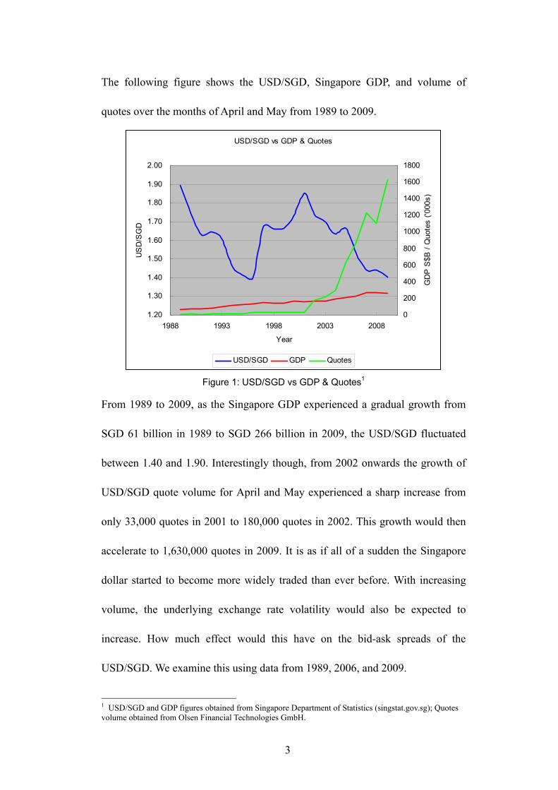
The following figure shows the USD/SGD, Singapore GDP, and volume of
quotes over the months of April and May from 1989 to 2009.
USD/SGD vs GDP & Quotes
1.20
1.30
1.40
1.50
1.60
1.70
1.80
1.90
2.00
1988 1993 1998 2003 2008
Year
US
D/S
GD
0
200
400
600
800
1000
1200
1400
1600
1800
GD
P S
$B /
Quo
tes
('000
s)
USD/SGD GDP Quotes
Figure 1: USD/SGD vs GDP & Quotes1
From 1989 to 2009, as the Singapore GDP experienced a gradual growth from
SGD 61 billion in 1989 to SGD 266 billion in 2009, the USD/SGD fluctuated
between 1.40 and 1.90. Interestingly though, from 2002 onwards the growth of
USD/SGD quote volume for April and May experienced a sharp increase from
only 33,000 quotes in 2001 to 180,000 quotes in 2002. This growth would then
accelerate to 1,630,000 quotes in 2009. It is as if all of a sudden the Singapore
dollar started to become more widely traded than ever before. With increasing
volume, the underlying exchange rate volatility would also be expected to
increase. How much effect would this have on the bid-ask spreads of the
USD/SGD. We examine this using data from 1989, 2006, and 2009.
1 USD/SGD and GDP figures obtained from Singapore Department of Statistics (singstat.gov.sg); Quotes volume obtained from Olsen Financial Technologies GmbH.

4
In 2006 the global economy had recorded a fourth consecutive year of strong
growth despite the drag from crude oil prices, a buildup in global electronics
inventories and adjustment in the US housing market. The MAS Annual Report
for 2005/2006 reported that “despite higher oil prices, rising interest rates and
natural disasters, the global economy expanded at a robust pace in 2005. This
growth momentum continued unabated in the first quarter of 2006. The strength
of the US economy was a major factor underpinning the continued growth of the
world economy last year. The US economy displayed remarkable resilience
against the backdrop of hurricane Katrina and 11 successive increases in the Fed
funds rate from 2.25% at the beginning of 2005 to 5% in May 2006. In the first
quarter of 2006, growth picked up strongly, led by a rebound in consumer
spending and business investment spending on equipment and software.”
The Singapore economy was also in a state of stability, as reported by the MAS
Annual Report 2005/2006: “In the early months of 2006, some signs of easing in
the domestic economy emerged with growth momentum slowing to 6.8% in Q1.
However, this is not indicative of a broad-based slowdown, but rather a
retraction to a more sustainable pace of growth.”
In 2009 the world found itself in the midst of the worst global financial crisis
ever since the Great Depression. The MAS Annual Report 2008/2009 reported
that “2008 was a tumultuous year for the global economy. While the surge in

5
commodity prices led to strong inflationary pressures in the first half of the year,
the onset of the global financial crisis caused world growth to fall sharply in the
later part of 2008 and into early 2009. The emergence of the Influenza A (H1N1)
virus in recent months has added a new dimension of risk to the fragile global
economy.”
The global financial crisis, which saw the collapse of Lehman Brothers in
September 2008, caused massive economic fallout worldwide. Amidst an
erosion of confidence, global trade and industrial production collapsed in the
first half of 2009, resulting in a 2.4% year-on-year contraction in world GDP
over the same period. During this time, the quote volume for USD/SGD (over
April and May) grew to over 1.6 million quotes, suggesting the increase in
volatility in the exchange rate.
1.2 The Microstructure Approach to Exchange Rate Economics
Exchange rate economics, the branch of international economics and finance
which attempt to explain the foreign exchange market, is an intriguing area of
research.
There are many theories of exchange rate determination, from the open economy
IS-LM models that are mandatory fare for any undergraduate economics course,
to more advanced models such as the Mundell-Fleming model, the

6
sticky/flexible-price monetary models, and the portfolio balance model. More
recently, new open-economy macroeconomists attempt for formalize exchange
rate in the context of dynamic general equilibrium models with explicit
microfoundations, nominal rigidities and imperfect competition.
When tested against empirical evidence, these theories have various degrees of
success in forecasting long-run exchange rates. All of them however are not able
to convincingly explain short-run exchange rate fluctuations.
From a common-sense perspective, this is hardly surprising. If the long-run
exchange rate between two countries is expected to change due to some shifting
fundamental value (say productivity level, for example), how would any macro
model (even one with microfoundations) designed to determine the “new”
equilibrium exchange rate be able to take into account all the possible paths
taken to transit from the “old” equilibrium rate to the “new” one? Some foreign
exchange transactions between the two countries might be related to shifting
fundamentals (e.g. import/export transactions), but others transactions may not
(e.g. tourism, speculation in each others’ asset markets, etc).
Macro foreign exchange models often assume that foreign exchange rates will
move when fundamentals move. But foreign exchange rates can only move
through a trading process in a foreign exchange market. Foreign exchange

7
microstructurists study this trading process.
In his book, “The Microstructure Approach to Exchange Rates”, Richard Lyons
(2001) defined “Order Flow” and “Bid-Ask Spreads”, two variables that are
absent from the macro approach, as the two hallmarks of the microstructure
approach. These are analogous to “Quantity” and “Price” in the dimension of
exchange rates.
Order flow is essentially transaction volume which is “signed”, meaning it
includes information if the transaction is a sale or a purchase. Such data is
usually hard to come by and are proprietary to banks and other high-level
participants in the foreign exchange market.
Well-connected researchers, such as Martin D. D. Evans and Richard K. Lyons
managed to obtain proprietary data on all end-user EUR/USD trades received at
Citibank over 6.5 years. In their 2007 paper “Exchange Rate Fundamentals and
Order Flow", they tested and established four empirical results: (1) transaction
flows forecast future macro variables such as output growth, money growth, and
inflation, (2) transaction flows forecast these macro variables significantly better
than the exchange rate does, (3) transaction flows (proprietary) forecast future
exchange rates, and (4) the forecasted part of fundamentals is better at
explaining exchange rates than standard measured fundamentals.

8
Data for the other hallmark, Bid-Ask Spreads, on the other hand, is much easier
to obtain. In fact, the four datasets for this paper were purchased from Olsen
Financial Technologies GmbH, while B&M obtained theirs by collecting every
USD/DEM quote posted on the Reuters screen for the interbank foreign
exchange market for three months in 1989. But other than being easily
obtainable, Lyons highlighted that one reason spreads receive so much attention
is because, being a core element of most data sets, they are a ready target for
testable hypotheses. This is in contrast to other features in the trading that are
not so easily measurable, such as information flow, belief dispersion, etc.
The behavior of bid-ask spreads in the foreign exchange markets offers many
opportunities for research. For example, Table 1 below shows the distribution of
over 600,000 USD/SGD quotes in April and May 2006, divided into nine
categories of price and spread movements.
SPREAD SPREAD SPREADUP SAME DOWN
PRICE UP 32.46% 6.35% 3.53%PRICE SAME 4.05% 7.52% 3.42%PRICE DOWN 3.21% 6.60% 32.85%
Total 39.73% 20.47% 39.81% Table 1: USD/SGD April-May 2006 Spread Behavior
Out of over 600,000 quotes over two months, the spread remained unchanged
6.35% of the time when the price moved up, and 6.60% of time when the price
moved down. Though we may somewhat expect for spreads to move when
prices move, what is intriguing is that when prices move up, spreads tended to
9
widen 32.46% of the time, but yet narrowed only 3.53% of the time, Conversely,
when prices move down, spreads tended to narrow 32.85% of the time but yet
widened only 3.21% of the time.
Spread behavior like in the previous example may differ across different
currencies within the same time period, and may also differ across different time
periods within the same currency. The empirical objective of this paper is thus to
examine the relationship between the bid-ask spread and the underlying
exchange rate volatility from such two angles. The main currency for analysis is
the USD/SGD. For comparison against a different currency within the same time
period, we use B&M’s results for the USD/DEM. For comparison against
different time periods within the same currency, we perform this analysis for the
USD/SGD from the months of April and May in 1989, 2006, and 2009. In
addition, we also perform an empirical analysis on the phenomenon described
above in Table 1.
1.3 Organization of Thesis
The rest of this paper shall be organized as follows: Chapter 2 begins with a
review of microstructure papers which concerns bid-ask spreads, and ends with
a description of B&M’s model that relates volatility to bid-ask spreads. Chapter
3 describes B&M’s empirical methodology and presents the empirical analyses
for each dataset. Chapter 4 concludes.

10
2 Bid-Ask Spreads in Exchange Rates
As previously mentioned in Chapter 1, Lyons (2001) cites bid-ask spreads as
one of the two hallmarks of the microstructure approach. Besides being
relatively obtainable, he explained that spreads receive so much attention
because they form a core element of most data sets and are a ready target for
testable hypotheses. He also gave two more reasons for the heavy attention and
resources focused on bid-ask spreads.
The second reason was because practitioners are “intensely concerned with
managing trading costs”. The third reason had to do with the history of the field
of market microstructure which in its early days sought to distinguish itself from
the literature on trading under rational expectations. Rational expectations
models generally omit trading mechanisms when characterizing the relationship
between fundamentals and price. Contrastingly market microstructure focused
on how trading mechanisms affected prices, and this had led to “a focus on the
determination of real-world transaction prices – spreads.”
For the first section of this Chapter, guided by Sarno & Taylor (2002), we
present a short survey on some early microstructure literature that concerns the
determination of bid-ask spreads, and focus on “adverse selection” as a popular
theme. We then present the views of a more contemporary paper which refutes

11
“adverse selection” as a determinant of bid-ask spreads and proposes that
asymmetric information might be a more plausible candidate.
From the second section of this Chapter we return to our main topic of interest –
bid-ask spreads and exchange rate volatility. Similarly, following Sarno &
Taylor (2002), we first present a short survey on the literature which analyses
the proportional relationship between spreads and exchange rate volatility.
We then close this Chapter by presenting B&M’s simple asymmetric
information model which forms the framework for our empirical investigation.
2.1 Bid-Ask Spreads and Asymmetric Information
Sarno & Taylor (2002) identifies three main determinants of the bid-ask spread:
the cost of dealer services, inventory holding costs, and the cost of adverse
selection.
Cost of Dealer Services
The cost of dealer services is formally analyzed by Demsetz (1968) who
assumes the existence of some fixed costs of providing “predictable immediacy”
as the service for which compensation is required by market makers. While
Demsetz focused on the New York Stock Exchange, his definition for cost of
dealer services could also be applicable to the foreign exchange market.

12
According to Demsetz, “predictable immediacy is a rarity in human actions, and
to approximate it requires that costs be borne by persons who specialize in
standing ready and waiting to trade with the incoming orders of those who
demand immediate servicing of their orders. The ask-bid spread is the markup
that is paid for predictable immediacy of exchange in organized markets; in
other markets, it is the inventory markup of retailer or wholesaler”.
Inventory Holding Costs
The original argument of inventory costs as a crucial determinant of bid-ask
spreads was first propositioned by Barnear & Logue (1975), who tested a
modified theory of market-maker behavior first espoused by Bagehot (1971).
Barnear & Logue modified the theory of the market-maker spread by
distinguishing between the two major components of inventory risk. The second
component, which they termed “marketability risk”, relates to the market
maker's ability to make inventory adjustments when the market for an issue is
"thin." They showed that volume has a negative effect on the bid-ask spread for
two reasons: 1) high volume implies more competition if it implies more
competition among alternative market makers; and 2) high volume implies less
marketability risk, and, therefore, lower positioning costs.
Amihud & Mendelson (1980) considers the problem of a price-setting
monopolistic market-maker in a Garman (1976) dealership market where the

13
stochastic demand and supply are depicted by independent Poisson processes.
The focus of their analysis is the dependence of the bid-ask prices on the
market-maker’s inventory position. They derived the optimal policy the results
are shown to be consistent with some conjectures and observed phenomena, like
the existence of a ‘preferred’ inventory position and the downward monotonicity
of the bid-ask prices.
Ho & Stoll (1981) considers the stochastic dynamic programming problem of
solving for the optimal behavior of a single dealer of a single stock who is faced
with a stochastic demand for his services and return risk on his stock and on the
rest of his portfolio. They show that as time unfolds and transactions occur, the
dealer is able to set his bid price and ask price relative to his opinion of the
"true" price of the stock so as to maximize the expected utility of terminal
wealth. The bid-ask spread is given by a risk neutral spread that maximizes
expected profits for the given stochastic demand functions plus a risk premium
that depends on transaction size, the return variance of the stock and the dealer's
attitude toward risk. The bid-ask spread does not depend on the dealer's
inventory position, but the dealer’s price adjustment does. When inventory
increases both bid price and ask price decline, and the converse is true when
inventory decreases.

14
Generally, inventory costs models assume that market-markers optimize their
inventory holding, and generally imply that market-makers shift the spread
downwards and increase the width of the spread when a positive inventory is
accumulated.
Cost of Adverse Selection
Adverse selection is a common argument to explain the existence of bid-ask
spreads. The origin of this argument could be traced back to Bagehot (1971),
whose model includes two types of market participants – those are willing to
pay the price of the spread to the market-maker in exchange for predictable
immediacy and those who can speculate at the expense of the market-maker
using some private insider information. An adverse selection arises because
market-makers are not able to distinguish between the two types of participants
and resort to widening the spreads for both types. The bid-ask spread then
becomes the market-maker’s defense against adverse selection in “in the form of
exploitation of arbitrage opportunities”. Since Bagehot, numerous
microstructure papers have drawn on adverse selection as their primary
interpretive framework.
Copeland & Galai (1983) analyses the determination of bid-ask spreads in
organized financial markets, where the trading is done through economic agents
who specialize in market-making for a limited set of securities. The commitment

15
made by dealers to buy or sell at the bid and ask prices, respectively, is analyzed
as a combination of put and call options. Given the behavior of liquidity traders
and informed traders, the dealer is assumed to offer an out-of-the-money
straddle option for a fixed number of shares during a fixed time interval. The
exercise prices of the straddle determine the bid-ask spread. The dealer
establishes his profit maximizing spread by balancing the expected total
revenues from liquidity trading against the expected total losses from informed
trading. They showed that a monopolistic dealer will establish a wider bid-ask
spread than will perfectly competitive dealers, and that the bid-ask spread
increases with greater price volatility in the asset being traded, with a higher
asset price level, and with lower volume.
Glosten & Milgrom (1985) analyzed a model of a securities market in which the
arrival of traders over time is accommodated by a market-maker. They showed
that adverse selection, by itself, could account for the existence of a bid-ask
spread, and the average magnitude of the spread depends on many parameters,
including the exogenous arrival patterns of insiders and liquidity traders, the
elasticity of supply and demand among liquidity traders, and the quality of the
information held by insiders. They also showed that, because transaction prices
are informative, bid-ask spreads tend to decline with trade.

16
Lyons (1995) was likely one of the first who departed from early microstructure
work that focused almost entirely on stock markets and applied such theory to
foreign exchange markets. He presented a model which incorporated a number
of institutional features relevant to the FX market, such as the facts that major
currencies are traded in decentralized dealership markets; that over 80% of the
trading volume is between market-makers; that market net volume is only
partially observable; and that customer order flow is an important source of
private information. Lyons showed that trade size and the bid-ask spreads of a
particular dealer were positively related.
Payne (2003) estimates a VAR decomposition of interdealer trades and quotes
and interprets the results through the lens of adverse selection. Specifically, he
used one trading week’s worth of USD/DEM data derived from an electronic
foreign exchange brokerage and employed the framework contained in
Hasbrouck & Sofianos (1993) to test for the existence of private information
effects of trading on prices. His basic results confirm the existence of private
information on FX markets, indicating that adverse selection costs account for
around 60% of the half-spread.
Osler, Mende & Menkhoff (2006) however shows evidence that the behavior of
bid-ask spreads is inconsistent with adverse selection. They outline three factors
that seem likely to be important. The first factor, fixed operating costs, can
17
explain the negative relation between trade size and bid-ask spreads if some
costs are fixed, but cannot explain the cross-sectional variation across customer
types. To explain why bid-ask spreads are larger for commercial than financial
customers they suggest that asymmetric information – in the broad sense of
information that is held by some but not all market participants – may influence
spreads through two channels distinct from adverse selection, one involving
market power and a second involving strategic dealing.
The market power hypothesis suggests that firms, even in a market with
hundreds of competitors like foreign exchange, gain market power from holding
information. It can be costly for customer firms to search out the best available
quotes in the foreign exchange market, so each individual dealer can exert a
certain amount of market power despite the competition. As suggested in Green
et al. (2005), dealers may quote the widest spreads when their market power is
greatest, and market power in quote-driven markets depends on knowledge of
current market conditions. In foreign exchange, commercial customers typically
know far less about market conditions than financial customers so they might be
expected to pay wider spreads, as they do.
The second channel through which asymmetric information might affect bid-ask
spreads in foreign exchange involves strategic dealing. Building on abundant
evidence that customer order flow carries information (e.g., Evans and Lyons
18
(2007), Daníelsson et al. (2002)), Osler et al argue that rational foreign exchange
dealers might strategically vary spreads across customers, subsidizing spreads to
informed customers in order to gain information which they can then exploit in
upcoming interbank trades. In standard adverse-selection models, by contrast,
dealers passively accept the information content of order flow. The idea that
dealers strategically vary spreads to gather information was originally explored
in Leach and Madhavan (1992, 1993). When applied to two-tier markets in Naik
et al. (1999) it implies that bid-ask spreads will be narrower for trades with
information, consistent with the pattern in foreign exchange.
2.2 Bid-Ask Spreads and Volatility
The directly proportional relationship between bid-ask spreads and exchange
rate volatility now represents a fairly stylized fact in the microstructure literature.
Early studies modeled the spread as a function of transaction costs, the bank’s
profit from providing liquidity services, and the market-maker’s payoff for
facing the exchange rate risk when assuming an open position. The main
conclusions of these early studies are that exchange rate spreads are wider under
floating exchange rate than under fixed-exchange rate regimes (e.g. Aliber,
1975), and that measures of exchange rate volatility are followed closely by
exchange rate spreads (e.g. Fieleke, 1975; Overturf, 1982).

19
Glassman (1987) provides a significant contribution to this literature in that she
builds a model where variables representing transactions frequency are included
explicitly and the non-normality of the distribution of exchange rates is taken
into account. The model not only provides additional evidence on the
proportional relationship between exchange rate volatility and bid-ask spreads in
the foreign exchange market, but also suggests that market-makers consider
moments of the exchange rate higher than the second moment in order to
evaluate the probability of large exchange rate changes.
Admanti & Pfleiderer (1988) provides another fundamental theoretical
contribution to this area. In their model, there are three types of agents: informed
traders, who have relatively superior information and only trade on terms
favorable to them; discretionary liquidity traders, who must trade during a day
but can choose when to trade during the day in order to minimize costs; and
non-discretionary liquidity traders, who must trade at a precise time during the
day regardless of the cost. In this model, trading volume is explained by the
concentration of trade of informed traders and discretionary liquidity traders at
certain points in time: the concentrations occur because it is profitable for
informed traders to trade when there are many liquidity traders who do not have
the same information as themselves and because discretionary liquidity traders
are attracted because the larger the number of traders lowers the cost of trading.

20
Bollerslev & Domowitz (1993) used intradaily data to investigate the behavior
of quote arrivals and bid-ask spreads. They recorded quote arrivals and bid-ask
spreads over the trading day, across geographical locations as well as across
market participants. They found that trading activity and the bid-ask spreads for
traders whose activity is restricted to regional markets can be described by a
U-shaped distribution, which is consistent with Admanti & Pfleiderer’s (1989)
model. The patterns of trading activity and spreads during the day also strongly
suggest some degree of traders’ risk aversion, given which, the more trading
activity is executed by informed traders, the higher the cost of trading.
Goodhart & Figliuoli (1991) reported a study of minute bid-ask quotes on three
days in 1987 at a Reuters screen and found evidence that leptokurtosis and
heteroscedasticity are time-varying, and are less pronounced at the
minute-by-minute frequency than at lower frequencies. They also found that
trading volume is time-varying, being higher at the European and North
American openings and lower at the European lunch hour. The series was also
found to exhibit first-order negative serial correlation, which is especially
pronounced after immediately after jumps in the exchange rate. Multivariate
analysis suggested significant relationships between lagged exchange rates and
the current spot rate.

21
2.3 Bollerslev & Melvin’s Model of Volatility and Bid-Ask Spread
B&M is the main inspiration for this thesis, providing most importantly a
methodology to analyze the relationship between bid-ask spreads of exchange
rates and its underlying volatility.
In the early 1990’s as B&M were writing their paper, the bid-ask spread
component of transactions costs in the foreign exchange market had not received
much attention in the literature. Earlier studies on the subject, such as Glassman
(1987) and Boothe (1988), concentrated on the own statistical properties of the
spread. Researchers, such as Goodhart (1990), Bossaerts and Hillion (1991),
Black (1991), Melvin and Tan (1996) and Bollerslev and Domowitz (1993), had
attempted to offer empirical and theoretical analyses of the determinants of
foreign exchange market spreads, but no one had performed any explicit
analysis of the relationship between the magnitude of foreign exchange market
spreads and the underlying exchange rate volatility. Hence, B&M is likely to be
the first paper to touch on this subject.
B&M opined that while unambiguous 'good' or 'bad' news regarding the
fundamentals of the exchange rate should have no systematic effect on the
spread, as both the bid and the ask prices should adjust in the same direction in
response to the traders receiving buy or sell orders that reflect the particular
news event, however greater uncertainty regarding the future spot rate, as

22
associated with greater volatility of the spot rate, is likely to result in a widening
of the spread.
We now outline B&M’s simple theoretical framework that illustrates this role of
volatility in determining the spread.
The formal setup for B&M’s stylized market microstructure model is based on
the analysis in Glosten and Milgrom (1985), Admati and Pfleiderer (1989), and
Andersen (1993).
The model assumes that the foreign exchange market comprises two kinds of
traders: liquidity traders and information-based traders. Liquidity traders
participate in foreign exchange transactions only due to the needs of their
normal business activity which require international trade of goods, services and
financial assets. They are also not speculators. Information-based traders profit
by intermediating the demands and supplies of foreign exchange for the liquidity
traders. These traders also take positions in the foreign exchange market based
on information advantages received through their dealings with the liquidity
traders or, more generally, information asymmetries regarding fundamentals
underlying the determination of the spot exchange rate.

23
The liquidity traders constitute the proportion (1— ) of the total market
participants. The liquidity traders receive a signal to either buy or sell foreign
currency regardless of the actual value of the currency in comparison with the
bid or ask prices prevailing at the time. Informed traders constitute the
remaining proportion of the market. This group of traders receives some
information about the true underlying fundamental value of the exchange rate st.
This fundamental value is assumed to evolve over time according to a
martingale model,
(1)
where Et-1( t)=0, Et-1( t2)= t
2, and Et-1(噝) denotes the conditional expectation
based on the information set generated by the past values of st. B&M further
assumes that the standardized innovations, t t-1, are independent and
symmetrically, but not necessarily identically, distributed through time.
At time t-1, one of the many market-making traders will set bid and ask quotes,
Bt and At, good for trading at time t. The bid-ask spread is assumed to be set
symmetrically around the known fundamental price prevailing at the time of
quote formation, i.e. At = st-1 + kt,t-1, and Bt = st-1 – kt,t-1. Thus, the quoted spread
for trades at time t, Kt = At, - Bt = 2kt,t-1 depends on time t-1 information only.

24
Trades at existing quotes will generate losses, on average, for the market-maker
when the opposite party an information-based trader. Information-based traders,
who received the signal t buy currency if At < st and sell currency if st, < Bt. For
values of Bt İ st İ�At, the information-based traders cannot profit from
knowing the true fundamental value revealed by t. The liquidity traders only
know st-1 and expect t to equal zero.
Trader positions are limited by the convention that existing quotes are only good
for up to some maximum quantity of currency. Assuming that the market-makers
limit trading to one unit of currency at existing quotes, the loss for the quoting
trader relative to the true value st arising from informed trading is therefore
(2)
Let Pt-1(噝) denote the probability conditional on the time t-1 information. Since
the standardized innovations, Zt = t t-1, are assumed to be independent and
symmetrically distributed through time, the expected loss from informed trading
may be expressed as
(3)

25
Assuming an equal probability of a buy or a sell order from the liquidity traders,
it follows that the expected profit for the quoting trader conditional on an
uninformed trade equals:
(4)
Combining the expected trading loss in Eq. (3) with the gain in Eq. (4) yields the
expected profit for the market-maker conditional on time t-1 information:
In equilibrium, competition from other banks or market-makers will drive this
expected profit to zero. Expressing this zero profit condition in terms of the total
spread, Kt =2kt,t-1 yields
(6)
Since the conditional expectation and probabilities on the right-hand side of Eq.
(6) only depend on the time t-1 information set through t-1kt,t-1, it follows that in

26
equilibrium the spread must move proportional to the conditional standard
deviation of the true fundamental value of the exchange rate.
B&M noted that while this simple proportionality condition would no longer
hold true in a more general model with endogenous information acquisition, the
result that an increase in t2 leads to an increase in Kt would still remain
generally valid.
Based on this relationship between exchange rate volatility and the bid-ask
spread, B&M designed the empirical methodology that we will describe in the
next chapter.

27
3 Empirical Analysis
B&M performed an empirical analysis on the USD/DEM, one of the most
highly-traded currency pair between two of the largest economies in the world in
1989 and showed that the size of the bid-ask spread of the USD/DEM is
positively related to its underlying exchange rate uncertainty. The USD/DEM is
a free-floating exchange rate. Their dataset consist of more than 300,000
continuously recorded USD/DEM quotes over a 3 month period from April to
June in 1989.
We are curious if 1) B&M’s result would hold for the USD/SGD, a semi-floating
currency from a much smaller economy, where over the same period from April
to May 1989, there were only slightly over 8,000 quotes; 2) B&M’s result would
hold 17 years later for that same currency, as that country becomes a significant
regional economic power in South-east Asia, and when the volume of quotes
increased to over 600,000 over April and May 2006.; and 3) B&M’s result
would hold as that economy enters into a period of worldwide financial crisis.
For the above purposes we purchased four sets of data from Olsen Financial
Technologies GmbH. Before we discuss the data and empirical results, we first
describe B&M’s empirical methodology and how we adapted it for this paper.

28
3.1 Empirical Methodology
B&M’s empirical methodology comprises two major steps.
Step 1: Creating a Proxy for Exchange Rate Volatility
The first step involves using a GARCH model as an explicit proxy for the
time-varying volatility of the spot rate, and as noted by Bollerslev et al. (1992),
such representations have been documented by numerous studies. B&M
employed a two-stage estimation procedure in which the conditional variance
for the spot exchange rate is first estimated as a GARCH process. These
estimates for the conditional variance are then used as the proxy for exchange
rate volatility in the second-stage model for the temporal behavior of the spread.
B&M use the ask price for estimation purposes; the bid and ask prices have
virtually identical higher order moments and differ only very slightly in their
conditional means. They found that the MA(1)-GARCH(1,1) model of the form
below seemed to fit their dataset well:
(7)
where It-1 denotes the time t-1 information set, and , , , , and are the
parameters to be estimated. The time t subscript refers to the place in the order

29
of the series of quotes, so that A,t2 provides an estimate of the price volatility
between quotes.
The particular specification for the conditional variance in Eq. (7) may be
justified by the theoretical arguments in Nelson (1990, 1992). Intuitively, if the
sample path for the true unobservable volatility process is continuous, it follows
that on interpreting the GARCH(1,1) model as a non-parametric estimator, or a
one-sided filter, the resulting estimates for the conditional variance will
generally be consistent as the length of the sampling interval goes to zero.
The primary purpose of the GARCH estimation was to create proxies for the
conditional variance of the exchange rate to be used in the investigation of the
determinants of the spread.
But it was 1993 then, and B&M noted that estimating a GARCH model with
more than 300,000 observations in practice was not feasible in practice. Hence,
they divided up their dataset into 12 weeks of data and estimated each set for the
above GARCH parameters. They then saved all the estimates for the conditional
variances from each of the 12 models and combined into a single time series of
volatility estimates for the full set of weekday quotes. Today, we use modern
econometrics software EViews to perform GARCH analysis on our datasets and
to obtain the conditional variance time series.

30
Step 2: Estimate Relationship between Spreads and Proxy for Volatility
The second major step of the methodology involved using ordered response
models to estimate the relationship between the time series of volatility
estimates obtained in the first step and the bid-ask spreads.
Specifically, B&M used an Ordered Probit model with multiplicative
heteroskedasticity for this purpose.
The observed spread, Kt, is assumed to take on only a fixed number of discrete
values, a1, a2, … aJ. The unobservable continuous random variable, K*, is
defined by
K*t = Xi’ + K,t (8)
The vector Xt denotes a set of predetermined variables that affect the conditional
mean of K*t and K,t, is conditionally normally distributed with mean zero and
variance, 2K,t
(9)
B&M allowed for multiplicative heteroskedasticity in the spread by
parameterizing the logarithm of 2K,t as a linear function of the same

31
explanatory variables that enter the conditional mean of K*t.
We depart from this path in our analysis, firstly by omitting multiplicative
heteroskedasticity (more due to the limitations of EViews than by choice), and
secondly by estimating the relationships with both Ordered Probit models and
Ordered Logit models (to allow more flexibility in the behaviour of the error
term, since we omitted multiplicative heteroskedasticity).
In our analyses, the observed spread, Kt, is similarly assumed to take on only a
fixed number of discrete values, a1, a2, … aJ, but the unobservable continuous
random variable, K*, is defined by
K*t = Xi’ + (10)
where is i.i.d. standard normal for the Ordered Probit model, and takes the
form of the logistic distribution for the Ordered Logit model.
The ordered response models relate the observed spreads to K* via
(11)
where the Aj’s form an ordered partition of the real line into J disjoint intervals.

32
The probability that the spread takes on the value aj is equal to the probability
that K* falls into the appropriate partition, Aj.
For tractability reasons, B&M based the empirical analysis on a classification of
the spread into only four different categories. From the distribution of spreads of
the USD/DEM in 1989, the four most commonly observed spreads account for
97.0 percent of the total quotes.
USD/DEMFrequency Distribution fof SpreadsSpread All Quotes0 < . < 5 2,304 (0.8%)5 77,856 (25.6%)5 < . < 7 607 (0.2%)7 34,878 (11.5%)7 < . < 10 2,977 (1.0%)10 170,892 (56.1%)10 < . < 15 329 (0.1%)15 11,534 (3.8%)15 < . < 20 39 (0.0%)20 2,616 (0.9%)20 < . 572 (0.2%)Note: Spreads converted into basis points
Table 2: Distribution of Spreads of USD/DEM April-June 1989
We also performed the ordered response analyses with four ordered indicator
values. In addition, as we will see later, because the spreads distribution for the
USD/SGD 2006 and 2009 data have more converging points (certain spread
sizes where there are more quotes than others) than both the USD/DEM and the
USD/SGD in 1989, we used up to 10 ordered indicator values in our own

33
ordered response analyses.
In the case of B&M where by four ordered indicator values of aj’s were used, the
corresponding intervals for the unobservable latent variable K* are defined by:
(12)
The partition parameters, I, are estimated jointly with the other parameters of
the model.
The ordered response model defined above allows us to estimate the probability
of a particular spread being observed as a function of the predetermined
variables, Xt. In order to test the hypothesis that the spread is partly determined
by the volatility of the spot rate, the GARCH estimate of the conditional
variance for the ask prices is included as one of the elements in Xt.
B&M noted that Bollerslev and Domowitz (1993) indicated a distinct intra-day
pattern in the spread distribution and tt is possible that any significant effect of
the conditional variance in isolation may merely reflect this dependence rather
than provide an independent influence on the spread process. In order to take
34
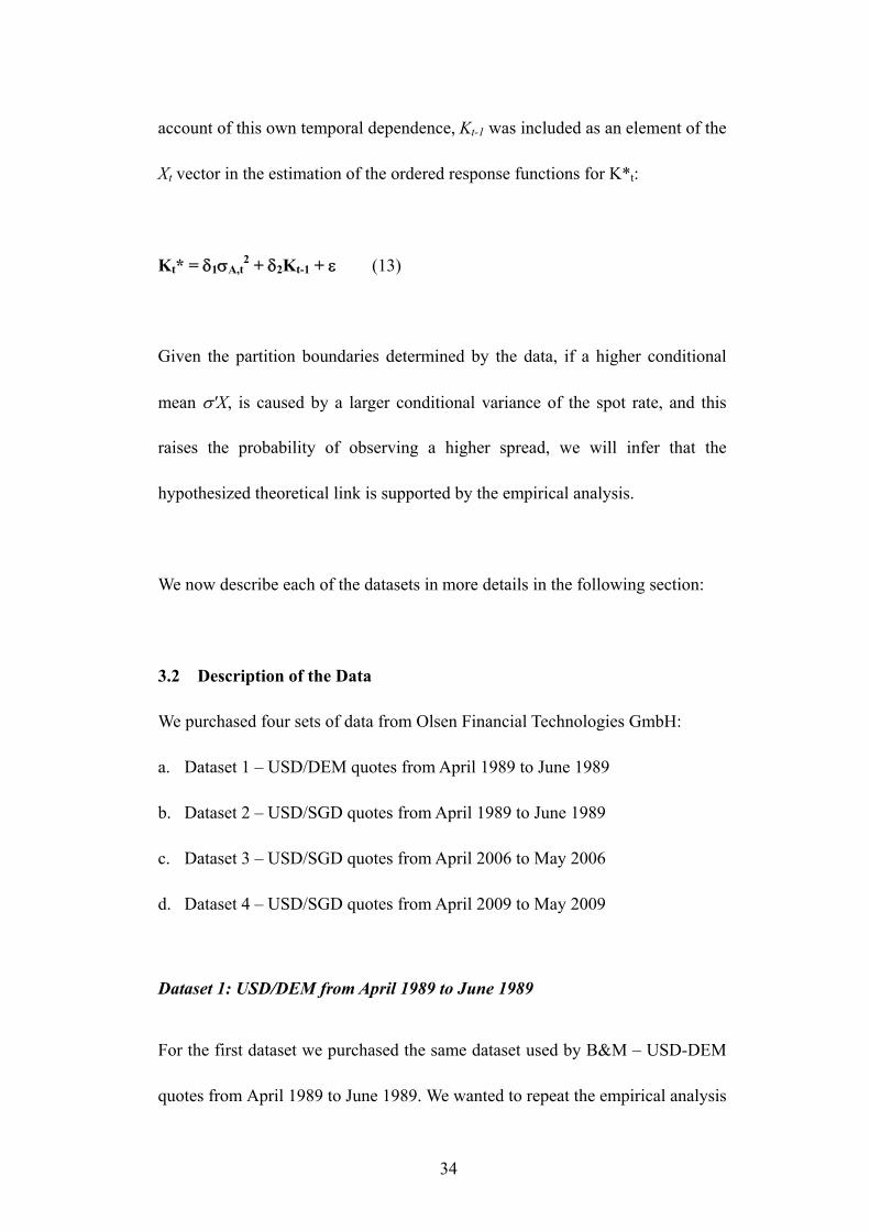
account of this own temporal dependence, Kt-1 was included as an element of the
Xt vector in the estimation of the ordered response functions for K*t:
Kt* = 1 A,t2 + 2Kt-1 + (13)
Given the partition boundaries determined by the data, if a higher conditional
mean 'X, is caused by a larger conditional variance of the spot rate, and this
raises the probability of observing a higher spread, we will infer that the
hypothesized theoretical link is supported by the empirical analysis.
We now describe each of the datasets in more details in the following section:
3.2 Description of the Data
We purchased four sets of data from Olsen Financial Technologies GmbH:
a. Dataset 1 – USD/DEM quotes from April 1989 to June 1989
b. Dataset 2 – USD/SGD quotes from April 1989 to June 1989
c. Dataset 3 – USD/SGD quotes from April 2006 to May 2006
d. Dataset 4 – USD/SGD quotes from April 2009 to May 2009
Dataset 1: USD/DEM from April 1989 to June 1989
For the first dataset we purchased the same dataset used by B&M – USD-DEM
quotes from April 1989 to June 1989. We wanted to repeat the empirical analysis
35
on the dataset again to allow for an apples-to-apples comparison between the
USD/DEM 1989 and the USD/SGD 1998 results.
First, B&M’s results were obtained in 1993 using probably not so
technologically advanced means. We wanted to repeat the estimation processes
again using EViews. Furthermore, as mentioned in the previous Chapter, we
departed from B&M’s ordered probit procedure by omitting multiplicative
heteroskedasticity. Second, B&M’s data were obtained from Reuters. From their
paper we were unable to ascertain the accuracy of this data, or how they
presented 12 workweeks of data from an actual 13 weeks in April to June 1989.
We obtained ours by purchasing from Olsen Financial Technologies GmbH and
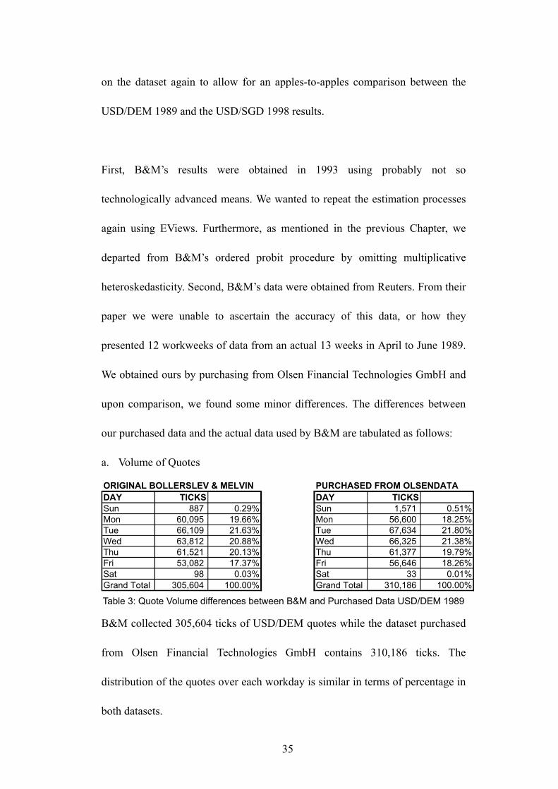
upon comparison, we found some minor differences. The differences between
our purchased data and the actual data used by B&M are tabulated as follows:
a. Volume of Quotes
ORIGINAL BOLLERSLEV & MELVIN PURCHASED FROM OLSENDATADAY TICKS DAY TICKSSun 887 0.29% Sun 1,571 0.51%Mon 60,095 19.66% Mon 56,600 18.25%Tue 66,109 21.63% Tue 67,634 21.80%Wed 63,812 20.88% Wed 66,325 21.38%Thu 61,521 20.13% Thu 61,377 19.79%Fri 53,082 17.37% Fri 56,646 18.26%Sat 98 0.03% Sat 33 0.01%Grand Total 305,604 100.00% Grand Total 310,186 100.00% Table 3: Quote Volume differences between B&M and Purchased Data USD/DEM 1989
B&M collected 305,604 ticks of USD/DEM quotes while the dataset purchased
from Olsen Financial Technologies GmbH contains 310,186 ticks. The
distribution of the quotes over each workday is similar in terms of percentage in
both datasets.

36
b. Frequency of No Spread Change
USD/DEMNo. of Quotes, & Frequency of No Spread Change
No Change in SpreadNumber Bid-Ask Rise Bid-Ask Fall
All quotes 304,619 8.00% 8.30% Table 4: Frequency of No Spread Change reported by B&M USD/DEM 1989
B&M reported that 8% of all the quotes observed no change in spread when the
bid-ask price rose and that 8.3% of all the quotes observed no change in spread
when the bid-ask price fell. It was not clear, however, whether these percentages
where calculated based on Number of Ticks with No Spread Change divided by
Number of Ticks Moved, or on Number of Ticks with No Spread Change
divided by Total Number of Ticks. We make this distinction clearer with the
purchased data.
SPREAD SPREAD SPREADUP SAME DOWN
PRICE UP 64384 32787 23767PRICE SAME 13083 39422 13523PRICE DOWN 24045 33407 64164Grand Total 101512 105616 101454
SPREAD SPREAD SPREADUP SAME DOWN
PRICE UP 53.24% 27.11% 19.65%PRICE SAME 19.81% 59.70% 20.48%PRICE DOWN 19.77% 27.47% 52.76%GRAND TOTAL 32.90% 34.23% 32.88%
SPREAD SPREAD SPREADUP SAME DOWN
PRICE UP 20.86% 10.63% 7.70%PRICE SAME 4.24% 12.78% 4.38%PRICE DOWN 7.79% 10.83% 20.79%GRAND TOTAL 32.90% 34.23% 32.88%
NO. OF QUOTES
DIVIDED BY NO OF TICKS MOVED
DIVIDED BY TOTAL NO. OF TICKS
Table 5: Frequency of No Spread Change with Olsen USD/DEM 1989
Among all ticks, we counted that 10.63% and 10.83% of all ticks observed no
change in spreads when the price rose and fell respectively.

37
c. Frequency Distribution of Spreads
Frequency Distribution of SpreadsSpread0 < . < 5 2,304 (0.8%) 2,562 (0.8%)5 77,856 (25.6%) 81,368 (26.4%)5 < . < 7 607 (0.2%) 660 (0.2%)7 34,878 (11.5%) 35,682 (11.6%)7 < . < 10 2,977 (1.0%) 3,192 (1.0%)10 170,892 (56.1%) 171,264 (55.5%)10 < . < 15 329 (0.1%) 327 (0.1%)15 11,534 (3.8%) 10,389 (3.4%)15 < . < 20 39 (0.0%) 38 (0.0%)20 2,616 (0.9%) 2,547 (0.8%)20 < . 572 (0.2%) 553 (0.2%)
ORIGINAL OLSENDATA
Note: Spreads converted into basis points Table 6: Frequency Distribution of Spreads USD/DEM 1989
It appears that the frequency distribution of spreads is quite similar between the
dataset reported by B&M and the dataset purchased from Olsen Financial
Technologies GmbH. The most common bid-ask spread is 10 basis points,
followed by 5 basis points.
Dataset 2: USD/SGD from April 1989 to June 1989
The second dataset are USD/SGD quotes from April 1989 to June 1989.
a. Volume of Quotes
DAY USD/SGDSun 6 0.07%Mon 1,307 15.43%Tue 2,024 23.89%Wed 1,876 22.14%Thu 1,652 19.50%Fri 1,586 18.72%Sat 21 0.25%Grand Total 8,472 100.00%
Table 7: Volume of Quotes of USD/SGD April-June 1989
Compared against a major currency in 1989 over the same period from April to
June, there are only 8,472 USD/SGD quotes compared to over 310,000 for the
USD/DEM. Distribution of the quotes over the week are however quite similar,
38
with volume peaking during midweek.
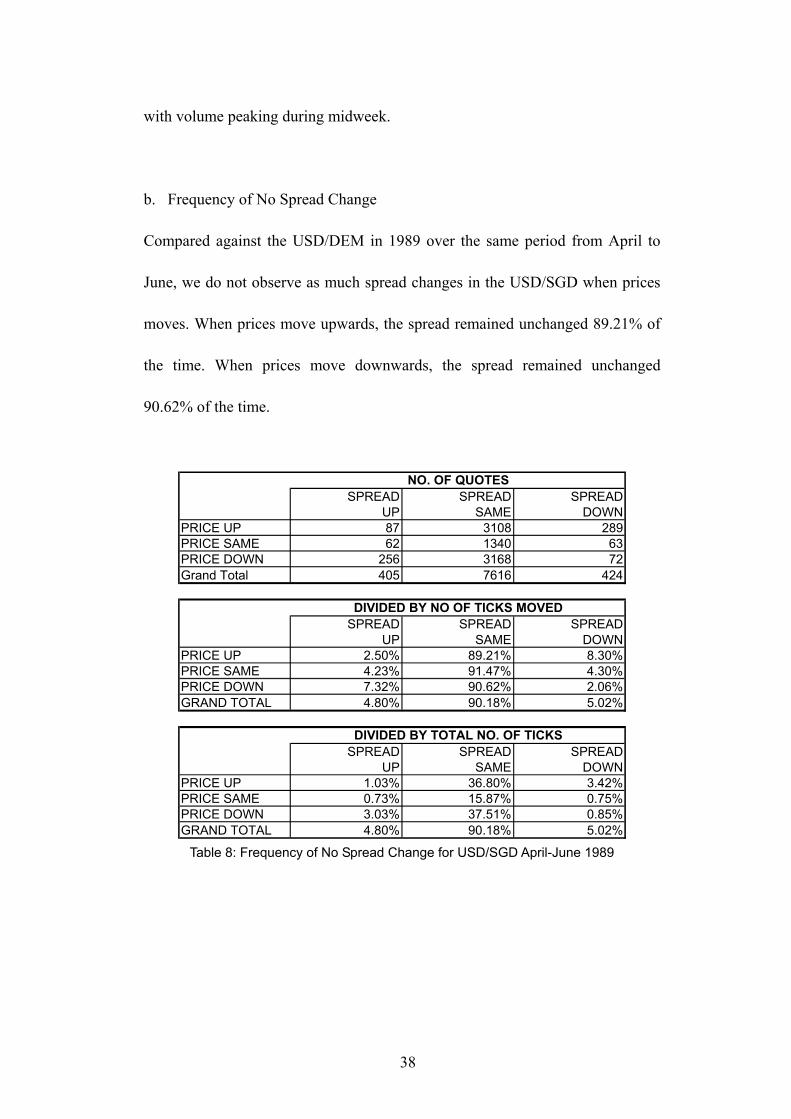
b. Frequency of No Spread Change
Compared against the USD/DEM in 1989 over the same period from April to
June, we do not observe as much spread changes in the USD/SGD when prices
moves. When prices move upwards, the spread remained unchanged 89.21% of
the time. When prices move downwards, the spread remained unchanged
90.62% of the time.
SPREAD SPREAD SPREADUP SAME DOWN
PRICE UP 87 3108 289PRICE SAME 62 1340 63PRICE DOWN 256 3168 72Grand Total 405 7616 424
SPREAD SPREAD SPREADUP SAME DOWN
PRICE UP 2.50% 89.21% 8.30%PRICE SAME 4.23% 91.47% 4.30%PRICE DOWN 7.32% 90.62% 2.06%GRAND TOTAL 4.80% 90.18% 5.02%
SPREAD SPREAD SPREADUP SAME DOWN
PRICE UP 1.03% 36.80% 3.42%PRICE SAME 0.73% 15.87% 0.75%PRICE DOWN 3.03% 37.51% 0.85%GRAND TOTAL 4.80% 90.18% 5.02%
NO. OF QUOTES
DIVIDED BY NO OF TICKS MOVED
DIVIDED BY TOTAL NO. OF TICKS
Table 8: Frequency of No Spread Change for USD/SGD April-June 1989

39
c. Frequency Distribution of Spreads
Frequency Distribution of SpreadsSpread0 < . < 5 6 (0.1%)5 137 (1.6%)5 < . < 7 22 (0.3%)7 122 (1.4%)7 < . < 10 43 (0.5%)10 7,854 (93.0%)10 < . < 15 6 (0.1%)15 76 (0.9%)15 < . < 20 1 (0.0%)20 164 (1.9%)20 < . 14 (0.2%)
USD/SGD
Note: Spreads converted into basis points Table 9: Frequency Distribution of Spreads USD/SGD April-June 1989
While spread changes in the USD/SGD are uncommon when prices moves, we
note similar characteristics to the USD/DEM in that the most common bid-ask
spread is 10 basis points. When spreads do change, they are most likely to be 5,
7 or 20 basis points.
Dataset 3: USD/SGD from April 2006 to May 2006
The third dataset are USD/SGD quotes from April 2006 to May 2006.
a. Volume of Quotes
DAY USD/SGDSun 3,832 0.63%Mon 104,327 17.24%Tue 126,812 20.96%Wed 147,084 24.31%Thu 135,037 22.32%Fri 87,332 14.44%Sat 555 0.09%Grand Total 604,979 100.00%
Table 10: Volume of Quotes of USD-SGD April-May 2006
15 years later, the USD/SGD has grown to become a major currency in
Southeast Asia. Compared against itself in 1989 over the period from April to
May, the volume of quotes of the USD/SGD has grown from over 8,400 ticks in
40
3 months to over 604,000 ticks in 2 months. The distribution of quotations over
the week remains consistent with volume peaking during midweek.
b. Frequency of No Spread Change
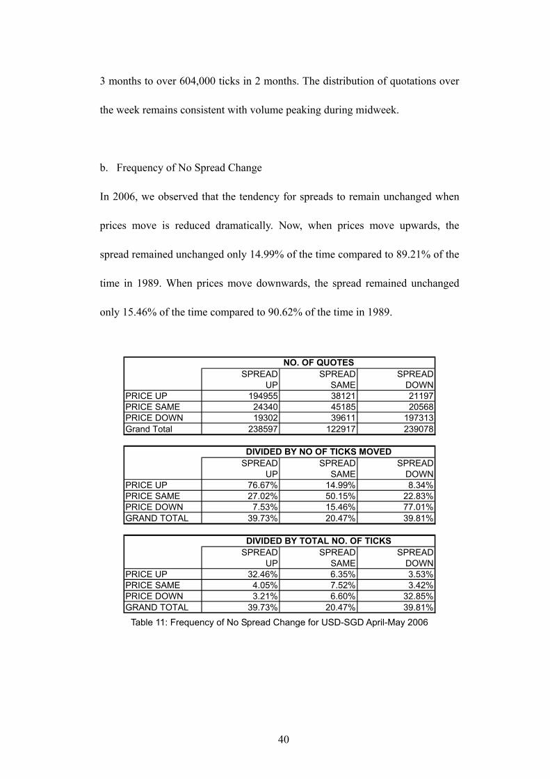
In 2006, we observed that the tendency for spreads to remain unchanged when
prices move is reduced dramatically. Now, when prices move upwards, the
spread remained unchanged only 14.99% of the time compared to 89.21% of the
time in 1989. When prices move downwards, the spread remained unchanged
only 15.46% of the time compared to 90.62% of the time in 1989.
SPREAD SPREAD SPREADUP SAME DOWN
PRICE UP 194955 38121 21197PRICE SAME 24340 45185 20568PRICE DOWN 19302 39611 197313Grand Total 238597 122917 239078
SPREAD SPREAD SPREADUP SAME DOWN
PRICE UP 76.67% 14.99% 8.34%PRICE SAME 27.02% 50.15% 22.83%PRICE DOWN 7.53% 15.46% 77.01%GRAND TOTAL 39.73% 20.47% 39.81%
SPREAD SPREAD SPREADUP SAME DOWN
PRICE UP 32.46% 6.35% 3.53%PRICE SAME 4.05% 7.52% 3.42%PRICE DOWN 3.21% 6.60% 32.85%GRAND TOTAL 39.73% 20.47% 39.81%
NO. OF QUOTES
DIVIDED BY NO OF TICKS MOVED
DIVIDED BY TOTAL NO. OF TICKS
Table 11: Frequency of No Spread Change for USD-SGD April-May 2006

41
c. Frequency Distribution of Spreads
Frequency Distribution of SpreadsSpread0 < . < 5 51,090 (8.5%)5 224,763 (37.2%)5 < . < 7 51,163 (8.5%)7 68,377 (11.3%)7 < . < 10 53,582 (8.9%)10 155,466 (25.7%)10 < . < 15 25 (0.0%)15 17 (0.0%)15 < . < 20 15 (0.0%)20 1 (0.0%)20 < . 0 (0.0%)
USD/SGD
Note: Spreads converted into basis points Table 12: Frequency Distribution of Spreads USD-SGD April-June 2006
The characteristics of the frequency distribution of spreads have also changed
almost completely over 15 years. The most common spread in 2006 is 5 basis
points, followed by 10 basis points. Most of the spreads recorded are either 10
basis points or lower, while quotes with spreads of more than 10 basis points
make up less than 0.01% of the entire spectrum of quotes.
Dataset 4: USD/SGD from April 2009 to May 2009
The fourth dataset are USD/SGD quotes from April 2009 to May 2009.
a. Volume of Quotes
DAY USD/SGDSun 9,336 0.87%Mon 183,055 17.02%Tue 217,496 20.22%Wed 237,508 22.08%Thu 237,604 22.09%Fri 190,603 17.72%Sat 32 0.00%Grand Total 1,075,634 100.00%
Table 13: Volume of Quotes of USD/SGD April-May 2009
In the year of the 2009 economic crisis, we observed a dramatic increase in
volume of USD-SGD quotes over the period of April to May 2009, as compared
to the same period in 2006, although we noted earlier that the volume growth
42
had been exponential since 2002. The volume of quotes of the USD-SGD has
grown from over 604,000 ticks, to exceeding 1 million quotes over a 2 month
period.
b. Frequency of No Spread Change
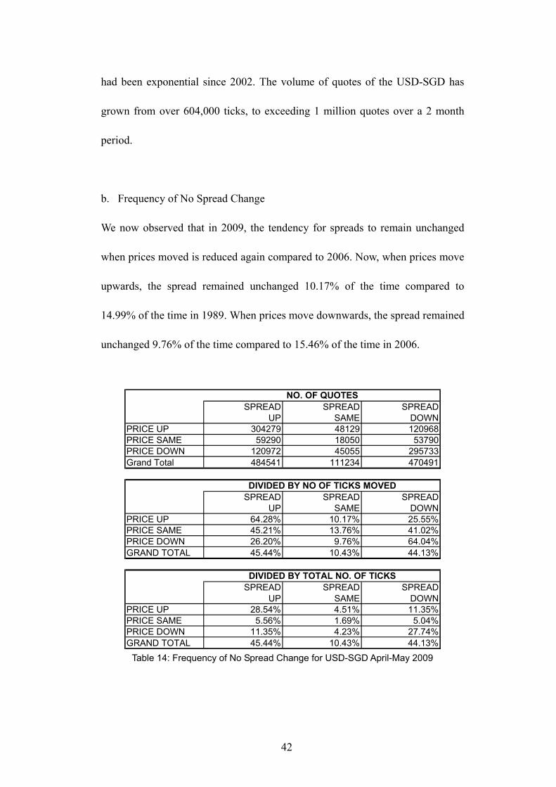
We now observed that in 2009, the tendency for spreads to remain unchanged
when prices moved is reduced again compared to 2006. Now, when prices move
upwards, the spread remained unchanged 10.17% of the time compared to
14.99% of the time in 1989. When prices move downwards, the spread remained
unchanged 9.76% of the time compared to 15.46% of the time in 2006.
SPREAD SPREAD SPREADUP SAME DOWN
PRICE UP 304279 48129 120968PRICE SAME 59290 18050 53790PRICE DOWN 120972 45055 295733Grand Total 484541 111234 470491
SPREAD SPREAD SPREADUP SAME DOWN
PRICE UP 64.28% 10.17% 25.55%PRICE SAME 45.21% 13.76% 41.02%PRICE DOWN 26.20% 9.76% 64.04%GRAND TOTAL 45.44% 10.43% 44.13%
SPREAD SPREAD SPREADUP SAME DOWN
PRICE UP 28.54% 4.51% 11.35%PRICE SAME 5.56% 1.69% 5.04%PRICE DOWN 11.35% 4.23% 27.74%GRAND TOTAL 45.44% 10.43% 44.13%
DIVIDED BY NO OF TICKS MOVED
DIVIDED BY TOTAL NO. OF TICKS
NO. OF QUOTES
Table 14: Frequency of No Spread Change for USD-SGD April-May 2009

43
c. Frequency Distribution of Spreads
Frequency Distribution of SpreadsSpread
<2.00 13 (0.0%)2 13,684 (1.3%)
2.00 < . < 3.00 8,422 (0.8%)3 54,432 (5.1%)
3.2 20,407 (1.9%)3.20 < . < 3.50 6,484 (0.6%)
3.5 114,907 (10.7%)3.50 < . < 4.00 10,882 (1.0%)
4 88,441 (8.2%)4.00 < . < 5.00 13,748 (1.3%)
5 59,572 (5.5%)5.00 < . < 6.00 6,932 (0.6%)
6 54,354 (5.1%)6.00 < . < 7.00 2,903 (0.3%)
7 165,828 (15.4%)7.00 < . < 8.00 2,080 (0.2%)
8 268,577 (25.0%)8.00 < . < 9.00 1,158 (0.1%)
9 39,789 (3.7%)9.00 < . < 10.00 830 (0.1%)
10 91,613 (8.5%)10.00 < . < 11.00 579 (0.1%)
11 11,304 (1.1%)> 11.00 38,696 (3.6%)
USD/SGD
Note: Spreads converted into basis points
Table 15: Frequency Distribution of Spreads USD-SGD April-May 2009
The characteristics of the frequency distribution of spreads have changed again
over 3 years. The most common spread in 2006 was 5 basis points, followed by
10 basis points. In 2009, the most common spread had risen to 8 basis points,
followed by 7 basis points and 3.5 basis points respectively. Most of the spreads
recorded are still either 10 basis points or lower, but quotations with spreads of
more than 10 basis points have increased to slightly under 5% of the entire
spectrum of quotations.
Two observations are of noteworthy regarding the 2009 dataset. First, the most
common spreads are no longer “significant” numbers such as 5 or 10. This could
indicate advancement in the market’s ability to evaluate foreign exchange risk,

44
and hence being able to price bids and asks more accurately. Second, the volume
of quotes with spreads of more than 10 basis points increased from 0.01% in
2006 to slightly under 5% in 2009. This could be attributed to the increased
amount of uncertainty in the financial markets during that period of global
economic crisis. Both phenomena could warrant future research.
3.3 GARCH Analysis
The primary purpose of the GARCH estimation was to create proxies for the
conditional variance of the exchange rate to be used in the investigation of the
determinants of the spread. Recall from Section 3.1 that, following B&M, we
estimate for each dataset with the following MA(1)-GARCH(1,1) model:
(7)
where It-1 denotes the time t-1 information set, and , , , , and are the
parameters to be estimated. The time t subscript refers to the place in the order
of the series of quotes, so that A,t2 provides an estimate of the price volatility
between quotes.
Following B&M, we first removed all weekend quotes. We then used EViews to
estimate the parameters for each dataset and the full results are attached in
45
Appendix 1. Here we present a summary of the results:
B&MDEM1989 DEM1989 SGD1989 SGD2006 SGD2009
0.0065 0.0069 0.0452 0.0025 0.0023(0.0042) (0.0013) (0.0138) (0.0004) (0.0003)
-0.5953 -0.5867 -0.3281 -0.7817 -0.7802(0.0052) (0.0014) (0.0114) (0.0009) (0.0006)
0.1008 0.0500 0.6833 0.0578 0.0453(0.0053) (0.0005) (0.0256) (0.0008) (0.0002)
0.0652 0.0561 0.2650 0.0632 0.0513(0.0018) (0.0003) (0.0081) (0.0006) (0.0002)
0.9057 0.9327 0.6540 0.9025 0.9197(0.0030) (0.0003) (0.0075) (0.0009) (0.0003)
0.9708 0.9888 0.9190 0.9657 0.9710304,608 308,748 8,444 551,355 1,006,736
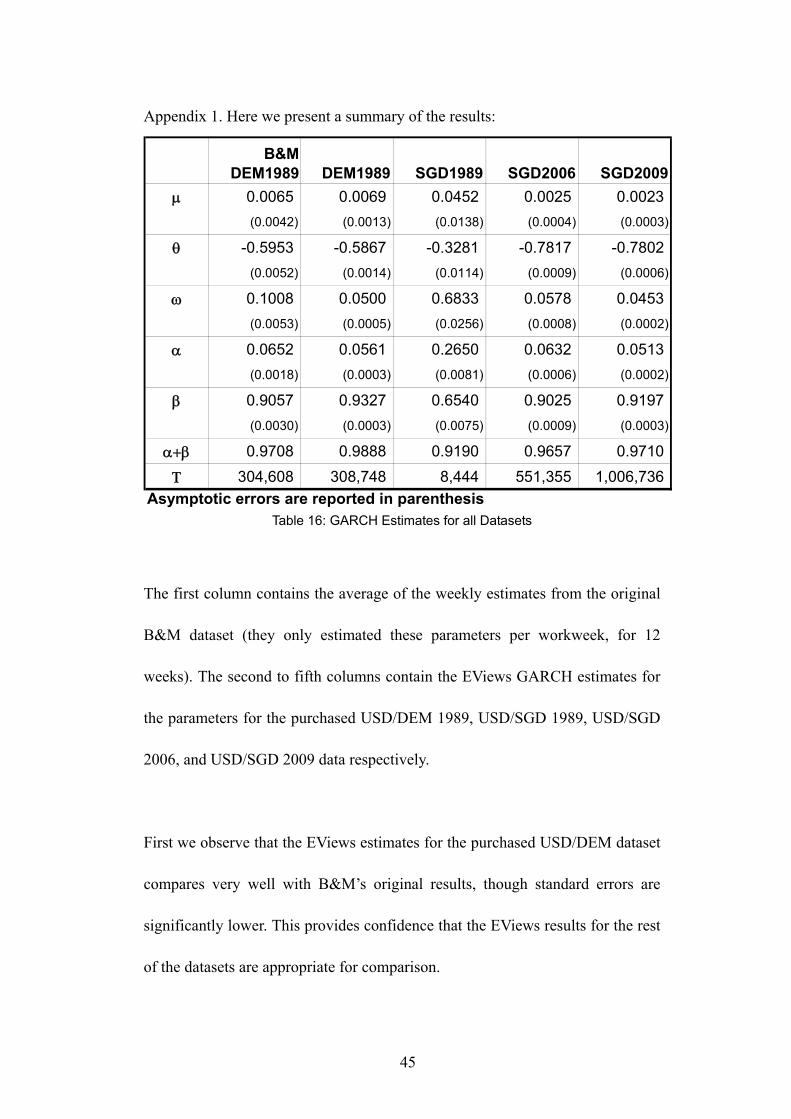
Asymptotic errors are reported in parenthesis Table 16: GARCH Estimates for all Datasets
The first column contains the average of the weekly estimates from the original
B&M dataset (they only estimated these parameters per workweek, for 12
weeks). The second to fifth columns contain the EViews GARCH estimates for
the parameters for the purchased USD/DEM 1989, USD/SGD 1989, USD/SGD
2006, and USD/SGD 2009 data respectively.
First we observe that the EViews estimates for the purchased USD/DEM dataset
compares very well with B&M’s original results, though standard errors are
significantly lower. This provides confidence that the EViews results for the rest
of the datasets are appropriate for comparison.

46
The second observation is that all estimates for are negative, which
corresponds to B&M’s results, and they noted that “the negative estimates for
may be partly attributed to a non-synchronous quoting phenomenon; see Lo and
MacKinlay (1990) for a formal analysis.”
The GARCH effects for all datasets are all highly significant. Comparing
GARCH effects between the USD/DEM 1989 dataset and USD/SGD 1989
dataset, it is clear that the USD/DEM dataset shows much stronger effects, and
stronger + volatility persistence. This is expected, as the USD/DEM dataset
contains at least 36 times more observations and from Table 8, the spread did not
change 90.18% of the time.
As the Singapore economy grows and the USD/SGD becomes a significant
regional currency, the results show that the GARCH effects and persistence of
volatility is consistent with this phenomenon.
The primary purpose of the GARCH estimation was to create proxies for the
conditional variance of the exchange rate to be used in the investigation of the
determinants of the spread. To this end, we used EViews to obtain GARCH
variance series for each dataset.

47
3.4 Ordered Response Analysis
Recall from Section 3.1 that we estimate for each dataset with the following
ordered response model (probit and logit):
Kt* = 1 A,t2 + 2Kt-1 + (13)
We first use four ordered indicator values and B&M’s definitions for aj’s:
a1: <= 5 a2: 5 < . < 10 a3: = 10 a4: > 10
The results for the above parameters for all four datasets are attached in
Appendix 1, but a summary is presented below:
DEM1989 SGD1989 SGD2006 SGD20090.0214 0.0091 0.0464 0.0988(73.9604) (10.6719) (29.2412) (113.8863)
0.3116 0.0422 -0.1306 0.2622(135.3568) (22.3298) -(69.4622) (177.1729)
308,748 8,444 551,355 1,006,736Z-statistics are reported in parenthesis
Table 17: Ordered Probit Estimates for all Datasets (4 ordered indicator values)
DEM1989 SGD1989 SGD2006 SGD20090.1299 0.0231 0.0802 0.2146
(102.6436) (9.2342) (28.9306) (109.5740)
0.4330 1.8160 -0.2040 0.4395(108.2955) (23.1592) -(66.7912) (169.4684)
308,748 8,444 551,355 1,006,736Z-statistics are reported in parenthesis
Table 18: Ordered Logit Estimates for all Datasets (4 ordered indicator values)

48
The positive 1 coefficients for both ordered probit and logit analyses above
suggest that there is a significantly positive effect of exchange rate volatility on
the spread for all datasets. The conditional mean of Kt* is an increasing function
of A,t2. This is consistent with the implications drawn from B&M’s theoretical
model. The estimates for 2 are indicative of intra-day persistence in the spread
process.
The magnitude of 1 for each dataset supports what we intuitively already know.
Comparing the USD/DEM and USD/SGD in 1989, although both 1 values are
statistically significant, volatility appears to play a much larger role in
determining the size of the spread for the USD/DEM. After all, as noted above,
the spread remained the same 90.18% of the time for the USD/SGD in 1989. For
the same reason, the 2 values show that the dependence on the previous spread
appears to be more significant for the USD/SGD than for the USD/DEM.
As the country grow in economic significance and the SGD becoming a major
regional currency over 17 years, the magnitude of the 1 values almost
quadrupled, coincidentally matching the growth in quote volume. It is
interesting to note the negative 2 values for the USD/SGD 2006 dataset, but it
might be due to seasonality.
49
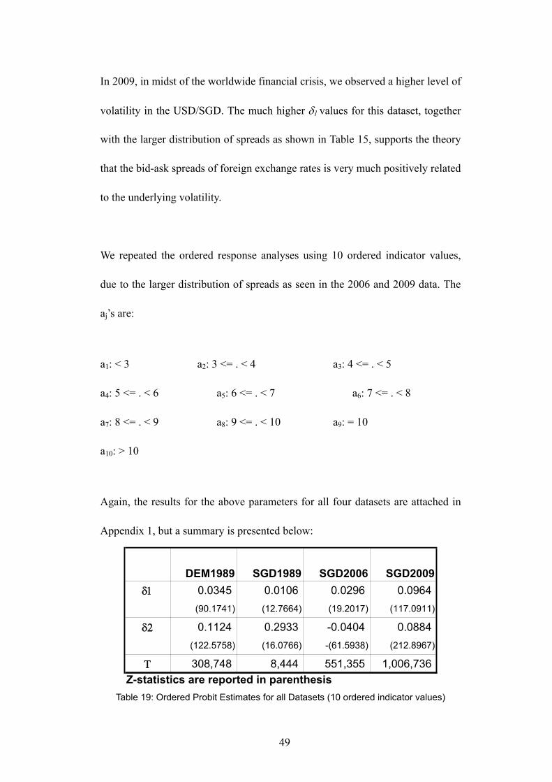
In 2009, in midst of the worldwide financial crisis, we observed a higher level of
volatility in the USD/SGD. The much higher 1 values for this dataset, together
with the larger distribution of spreads as shown in Table 15, supports the theory
that the bid-ask spreads of foreign exchange rates is very much positively related
to the underlying volatility.
We repeated the ordered response analyses using 10 ordered indicator values,
due to the larger distribution of spreads as seen in the 2006 and 2009 data. The
aj’s are:
a1: < 3 a2: 3 <= . < 4 a3: 4 <= . < 5
a4: 5 <= . < 6 a5: 6 <= . < 7 a6: 7 <= . < 8
a7: 8 <= . < 9 a8: 9 <= . < 10 a9: = 10
a10: > 10
Again, the results for the above parameters for all four datasets are attached in
Appendix 1, but a summary is presented below:
DEM1989 SGD1989 SGD2006 SGD20090.0345 0.0106 0.0296 0.0964(90.1741) (12.7664) (19.2017) (117.0911)
0.1124 0.2933 -0.0404 0.0884(122.5758) (16.0766) -(61.5938) (212.8967)
308,748 8,444 551,355 1,006,736Z-statistics are reported in parenthesis
Table 19: Ordered Probit Estimates for all Datasets (10 ordered indicator values)

50
DEM1989 SGD1989 SGD2006 SGD20090.1557 0.0305 0.0599 0.2047
(115.2591) (10.8283) (22.1246) (110.9948)
0.1599 0.5637 -0.0755 0.1493(100.3382) (16.7295) -(67.7863) (205.0571)
308,748 8,444 551,355 1,006,736Z-statistics are reported in parenthesis
Table 20: Ordered Logit Estimates for all Datasets (10 ordered indicator values)
Generally, the conclusions from the previous ordered response analyses with 4
ordered indicator values still holds after we attempt to be more discerning with
the ordered indicator values.
3.5 Incorporating Returns
Recall that we noted (see Tables 5, 11 and 14) an interesting phenomenon
regarding the behavior of bid-ask spreads of foreign exchange rates. When
prices move up, and the bid-ask spreads change, they tend to widen. Conversely,
when prices move down, and the bid-ask spreads change, they tend to narrow.
Previously we were examining the relationship between bid-ask spreads and the
underlying volatility of exchange rates and found that positive relationships
generally exists between the two. We are now curious if there is any relationship
between bid-ask spreads and price movement. To examine this we repeat the
ordered response analyses by including the Returns variable from the
MA(1)-GARCH(1,1) model into the ordered response model:

51
Kt* = 1 A,t2 + 2Kt-1 + 310,000* logAt + (14)
We repeated the ordered probit and ordered logit analyses for all four datesets
using both 4 and 10 ordered indicator values. The results are attached in
Appendix 1, but we summarize the results below:
DEM1989 SGD1989 SGD2006 SGD20090.0148 0.0093 0.0325 0.0406(51.4649) (10.9454) (19.1288) (44.7718)
0.0383 1.0090 0.5203 0.2606(16.2662) (23.4338) (210.7702) (146.0215)
0.0970 0.0827 0.6241 0.4158(98.3419) (12.2743) (449.5486) (437.6876)
308,748 8,444 551,355 1,006,736Z-statistics are reported in parenthesis
Table 21: Ordered Probit Estimates (with Returns) for all Datasets (4 ordered values)
DEM1989 SGD1989 SGD2006 SGD20090.1319 0.0235 0.0485 0.2225
(101.6830) (8.7724) (14.8530) (96.1127)
0.6732 1.9380 1.0532 1.9644(154.6104) (24.1228) (229.6602) (494.6543)
0.3205 0.1796 1.2152 1.3865(174.0656) (12.2520) (409.7483) (585.1713)
308,748 8,444 551,355 1,006,736Z-statistics are reported in parenthesis
Table 22: Ordered Logit Estimates (with Returns) for all Datasets (4 ordered values)
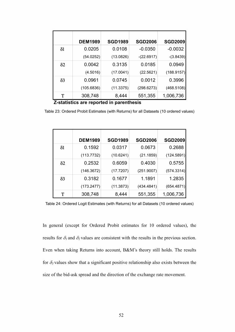
52
DEM1989 SGD1989 SGD2006 SGD20090.0205 0.0108 -0.0350 -0.0032(54.0252) (13.0826) -(22.6917) -(3.8439)
0.0042 0.3135 0.0185 0.0949(4.5016) (17.0041) (22.5621) (188.9157)
0.0961 0.0745 0.0012 0.3996(105.6836) (11.3375) (298.6273) (468.5108)
308,748 8,444 551,355 1,006,736Z-statistics are reported in parenthesis
Table 23: Ordered Probit Estimates (with Returns) for all Datasets (10 ordered values)
DEM1989 SGD1989 SGD2006 SGD20090.1592 0.0317 0.0673 0.2688
(113.7732) (10.6241) (21.1859) (124.5891)
0.2532 0.6059 0.4030 0.5755(146.3672) (17.7207) (251.9007) (574.3314)
0.3182 0.1677 1.1891 1.2835(173.2477) (11.3873) (434.4841) (654.4871)
308,748 8,444 551,355 1,006,736 Table 24: Ordered Logit Estimates (with Returns) for all Datasets (10 ordered values)
In general (except for Ordered Probit estimates for 10 ordered values), the
results for 1 and 2 values are consistent with the results in the previous section.
Even when taking Returns into account, B&M’s theory still holds. The results
for 3 values show that a significant positive relationship also exists between the
size of the bid-ask spread and the direction of the exchange rate movement.

53
One interesting result to note are the negative 1 and 2 values for the ordered
probit analyses of 2006 and 2009 for 10 ordered indicator values (see Table 23).
Not only does this violate B&M’s prediction, the observation that the 1 values
appear to decrease with increasing tick volume runs counter to the rest of the
ordered response results. One possible explanation for this is that multiplicative
heteroskedasticity, which our ordered response models omitted but has been
shown to be significant by B&M, is likely to be the cause of this results.
Also since we know that the error term of equations 13 and 14 are not i.d.d.
standard normal, the results for the ordered logit analyses are probably more
meaningful.
3.6 Summary
B&M provided the theoretical framework and showed empirical evidence that
the size of the bid-ask spread of exchange rates is positively related to the
exchange rate’s underlying volatility. Their empirical subject was over 300,000
USD/DEM quotes from April to June of 1989. The USD/DEM was obviously
one of the most traded currency pair during that time, and both the USD and
DEM belonged to floating exchange rates regimes of two of the top three largest
world economies in 1989.

54
We then wanted to see if both theory and empirical results would hold for a
much lesser traded subject currency, if the currency belonged to a small country
and from a semi-floating exchange rate regime – the USD/SGD.
We applied a modified version of B&M’s methodology on the USD/SGD from
the same months of April to June 1989 and found that the evidence (as
documented in the previous section) supported their theory. Furthermore, we
repeated the analysis on the USD/SGD 17 years later in 2006 when the world
economy was at a point of stability, and again in 2009 when the world economy
was somewhat in disarray. We found that B&M’s theory was still supported by
the evidence.
Along the way we also noted the interesting phenomenon regarding the behavior
of bid-ask spreads of foreign exchange rates. When prices move up, and the
bid-ask spreads change, they tend to widen. Conversely, when prices move
down, and the bid-ask spreads change, they tend to narrow. We repeated the
analyses on the datasets and included Returns as additional variable in the
ordered response models. We found that the relationship between bid-ask
spreads and price direction is positive and significant.

55
4 Conclusion
This paper has set out to empirically test B&M’s theory against a lesser-traded
currency from a developing country with a managed floating rate regime. The
results generally hold, and we found that the effects of the tested parameters
grew in strength as that currency grew in economic significance in its region.
We departed from B&M’s methodology by omitting multiplicative
heteroskedasticity, but we tested our data using both Ordered Probit and Ordered
Logit models. The generally “better-behaving” results from the Logit models
suggests that the disturbances are indeed not standard normal, and that future
work in this area using the same methodologies should include multiplicative
heteroskedasticity.
We also noted the interesting phenomenon regarding the behavior of bid-ask
spreads of foreign exchange rates. We included returns as additional variable in
the ordered response models and found that the relationship between bid-ask
spreads and price direction is positive and significant. Future work in this area
should attempt to build a model which links bid-ask spreads not only to
volatility and also returns.
We provided a simple survey on microstructure literature. We first touched on
those which analyses bid-ask spreads and asymmetric information, and also

56
presented snapshots of research involving bid-ask spreads and volatility. Bid-ask
spreads, one of two “hallmarks” of the microstructure approach, remain a
popular theme for research today.
57
References Admanti, A., and Pfleiderer, P., (1988), “A Theory of Intraday Patterns: Volume and
Price Variability,” Review of Financial Studies, 1, pp. 3-40 Admanti, A.R. and Pfleiderer, P., (1989), “Divide and Conquer: A Theory of
Intra-day and Day of the Week Effects,” Review of Financial Studies, 2, pp. 189-223
Aliber, R.Z., (1975), “Monetary Independence under Floating Exchange Rates,”
Journal of Finance, 30, pp. 365-376 Amihud, Y. and Mendelson, H. (1980), “Dealership Market: Market-making with
Inventory”, Journal of Financial Economics, pp. 31-53 Bagehot, W. (1971), “The Only Game in Town,” Financial Analysts Journal, 22, pp.
12-14 Barnea, A. and Logue, D.E. (1975), “The Effect of Risk on the Market Maker’s
Spread”, Financial Analysts Journal, 31, pp. 45-49 Black, S.W., (1991), “Transactions Costs and Vehicle Currencies,” Journal of
International Money and Finance, 10, pp. 512-526 Bollerslev, T., Chou, R.Y., and Kroner, K.F., (1992), “ARCH Modeling in Finance:
A Review of the Theory and Empirical Evidence,” Journal of Econometrics, 52, pp. 5-59
Bollerslev, T., and Domowitz, I., (1993), “Trading Patterns and Prices in the
Interbank Foreign Exchange Market,” Journal of Finance, 48, pp. 1421-1443 Bollerslev, T. and Melvin, M. (1994), “Bid-ask Spreads and Volatility in the Foreign
Exchange Market – an Empirical Analysis,” Journal of International Economics, 36, pp. 355-372
Boothe, P., (1988), “Exchange Rate Risk and the Bid-Ask Spread: A Seven Country
Comparison,” Economic Inquiry, 26, pp. 485-492 Bossaerts, P. and Hillion, P., (1991), “Market Microstructure Effects of Government
Intervention in the Foreign Exchange Market,” Review of Financial Studies, 4, pp. 513-541
Copeland, T. and Galai, D. (1983), “Information Effects on the Bid-Ask Spread,”
58
Journal of Finance, 38, pp. 1457-1469 Demsetz, H (1968), “The Cost of Transacting”, Quarterly Journal of Economics, 82,
pp. 33-53 Evans, M. and Lyons, R. (2007), “Exchange Rate Fundamentals and Order Flow,”
NBER Working Papers 13151, National Bureau of Economic Research, Inc. Fieleke, N.S., (1975), “Exchange Rate Flexibility and the Efficiency of Foreign
Exchange Markets,” Journal of Financial and Quantitative Analysis, 10, pp. 409-428
Glassman, D.A., (1987), “Exchange Rate Risks and Transaction Costs: Evidence
from Bid-Ask Spreads,” Journal of International Money and Finance, 6, pp. 479-490
Glosten, L.R. and Milgrom, P.R. (1985), “Bid, Ask and Transaction Prices in a
Specialist Market with Heterogeneously Informed Traders,” Journal of Financial Economics, 14, pp. 71-100
Goodhart, C.A.E., and Figliuoli, L., (1991), “Every Minute Counts in Financial
Markets,” Journal of International Money and Finance, 10, pp. 23-52 Goodhart, C.A.E., (1990), “News and the Foreign Exchange market,” FMG
Discussion Papers dp71, Financial Markets Group Green, R., Hollified, B. and Schurhoff, N. (2005), “Financial Intermediation And
The Costs Of Trading In An Opaque Market,” FAME Research Paper Series rp130, International Center for Financial Asset Management and Engineering
Hasbrouck, J. and Sofianos, G.. (1993), “The Trades Of Market Makers: An
Empirical Analysis Of NYSE Specialists,” Journal of Finance, 48, pp. 1565-1593.
Ho, T. and Stoll, H. (1981), “Optimal Dealer Pricing under Transactions and Return
Uncertainty,” Journal of Financial Economics, 9, pp. 757-84 Leach, C.J., and Madhavan, A.N., (1992), “Intertemporal Price Discovery By
Market Makers: Active Versus Passive Learning,” Journal of Financial Intermediation, 2, pp. 207-235
Leach, C.J., and Madhavan, A.N., (1993), “Price Experimentation And Security
Market Structure”, Review of Financial Studies, 6, pp. 375-404

59
Lo, A.W. and Mackinlay, A.C., (1990), “An Econometric Analysis of Non-Synchronous Trading,” Journal of Econometrics, 45, pp. 181-210
Lo, A.W., and MacKinlay, A.C., (1992), “An Ordered Probit Analysis of
Transaction Stock Prices,” Journal of Financial Economics, 31, pp. 319-379 Lyons, R. (1995), “Tests of Microstructural Hypotheses in the Foreign Exchange
Market”, Journal of Financial Economics, 39, pp. 321-351 Lyons, R. (2001) The Microstructure Approach to Exchange Rates, The MIT Press,
Cambridge, MA Melvin, M. and Tan, K.H., (1996), “Foreign Exchange Market Bid-Ask Spreads and
the Market Price of Social Unrest,” Oxford Economic Papers, Oxford University Press, 48(2), pp. 329-41
Monetary Authority of Singapore Annual Report 2005/2006 Monetary Authority of Singapore Annual Report 2008/2009 Naik, N.Y., Neuberger, A. and Viswanathan, S., (1999), “Trade Disclosure
Regulation In Markets With Negotiated Trades,” Review of Financial Studies, 12, pp. 873-900
Nelson, D.B., (1990), “ARCH Models as Diffusion Approximations,” Journal of
Econometrics, 45, pp. 7-38 Nelson, D.B., (1992), “Filtering and Forecasting with Misspecified ARCH Models I:
Getting the Right Variance with the Wrong Model,” Journal of Econometrics, 52, pp. 61-90
Osler, C., Mende, A. and Menkhoff, L. (2006), “Price Discovery in Currency
Markets,” Diskussionspapiere der Wirtschaftswissenschaftlichen Fakultät der Universität Hannover dp-351, Universität Hannover, Wirtschaftswissenschaftliche Fakultät.
Overturf, S.F., (1982), “Risk, Transaction Charges, and the Market for Foreign
Exchange Services,” Economic Inquiry, 20, pp. 291-302 Payne, R. (2003), “Informed Trade In Spot Foreign Exchange Markets: An
Empirical Investigation,” Journal of International Economics, 61, pp. 307-329 Sarno, L. and Taylor M. (2002) The Exconomics of Exchange Rates Cambridge
University Press, Cambridge, UK
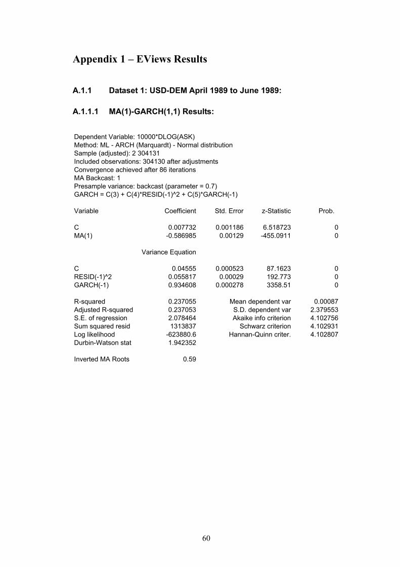
60
Appendix 1 – EViews Results
A.1.1 Dataset 1: USD-DEM April 1989 to June 1989:
A.1.1.1 MA(1)-GARCH(1,1) Results:
Dependent Variable: 10000*DLOG(ASK)Method: ML - ARCH (Marquardt) - Normal distributionSample (adjusted): 2 304131Included observations: 304130 after adjustmentsConvergence achieved after 86 iterationsMA Backcast: 1Presample variance: backcast (parameter = 0.7)GARCH = C(3) + C(4)*RESID(-1)^2 + C(5)*GARCH(-1)
Variable Coefficient Std. Error z-Statistic Prob.
C 0.007732 0.001186 6.518723 0MA(1) -0.586985 0.00129 -455.0911 0
Variance Equation
C 0.04555 0.000523 87.1623 0RESID(-1)^2 0.055817 0.00029 192.773 0GARCH(-1) 0.934608 0.000278 3358.51 0
R-squared 0.237055 Mean dependent var 0.00087Adjusted R-squared 0.237053 S.D. dependent var 2.379553S.E. of regression 2.078464 Akaike info criterion 4.102756Sum squared resid 1313837 Schwarz criterion 4.102931Log likelihood -623880.6 Hannan-Quinn criter. 4.102807Durbin-Watson stat 1.942352
Inverted MA Roots 0.59

61
A.1.1.2 Ordered Probit Results: 4 Ordered Values
Dependent Variable: AJMethod: ML - Ordered Probit (Quadratic hill climbing)Sample (adjusted): 2 304131Included observations: 304130 after adjustmentsNumber of ordered indicator values: 4Convergence achieved after 4 iterationsCovariance matrix computed using second derivatives
Variable Coefficient Std. Error z-Statistic Prob.
GARCHVAR 0.021372 0.000289 73.96036 0AJ(-1) 0.311626 0.002302 135.3568 0
Limit Points
LIMIT_2:C(3) 0.190472 0.005775 32.98297 0LIMIT_3:C(4) 0.557843 0.005798 96.21363 0LIMIT_4:C(5) 2.633627 0.007509 350.7163 0
Pseudo R-squared 0.041442 Akaike info criterion 2.077312Schwarz criterion 2.077487 Log likelihood -315881.5Hannan-Quinn criter. 2.077363 Restr. log likelihood -329538.1LR statistic 27313.29 Avg. log likelihood -1.03864Prob(LR statistic) 0

62
A.1.1.3 Ordered Probit (with Returns) Results: 4 Ordered Values
Dependent Variable: AJMethod: ML - Ordered Probit (Quadratic hill climbing)Sample (adjusted): 2 304131Included observations: 304130 after adjustmentsNumber of ordered indicator values: 4Failure to improve Likelihood after 12 iterationsCovariance matrix computed using second derivatives
Variable Coefficient Std. Error z-Statistic Prob.
GARCHVAR 0.014821 0.000288 51.46485 0AJ(-1) 0.038314 0.002355 16.26616 010000*DLOG(ASK) 0.096973 0.000986 98.34188 0
Limit Points
LIMIT_2:C(4) -0.569596 0.005843 -97.47589 0LIMIT_3:C(5) -0.204094 0.005933 -34.39776 0LIMIT_4:C(6) 1.828335 0.007386 247.5462 0
Pseudo R-squared 0.041202 Akaike info criterion 2.077839Schwarz criterion 2.078049 Log likelihood -315960.6Hannan-Quinn criter. 2.0779 Restr. log likelihood -329538.1LR statistic 27155.04 Avg. log likelihood -1.0389Prob(LR statistic) 0

63
A.1.1.4 Ordered Probit Results: 10 Ordered Values
Dependent Variable: AJMethod: ML - Ordered Probit (Quadratic hill climbing)Sample (adjusted): 2 308749Included observations: 307943 after adjustmentsNumber of ordered indicator values: 10Convergence achieved after 7 iterationsCovariance matrix computed using second derivatives
Variable Coefficient Std. Error z-Statistic Prob.
GARCHVAR 0.034469 0.000382 90.17413 0AJ(-1) 0.112367 0.000917 122.5758 0
Limit Points
LIMIT_2:C(3) -2.206482 0.01721 -128.2094 0LIMIT_3:C(4) -1.756869 0.010998 -159.7475 0LIMIT_4:C(5) -1.538779 0.00944 -162.9984 0LIMIT_5:C(6) 0.322974 0.006894 46.85067 0LIMIT_6:C(7) 0.329696 0.006894 47.8258 0LIMIT_7:C(8) 0.666276 0.006924 96.2254 0LIMIT_8:C(9) 0.693844 0.006929 100.1396 0LIMIT_9:C(10) 0.694678 0.006929 100.2579 0LIMIT_10:C(11) 2.788901 0.008505 327.928 0
Pseudo R-squared 0.037526 Akaike info criterion 2.258734Schwarz criterion 2.259114 Log likelihood -347769.7Hannan-Quinn criter. 2.258844 Restr. log likelihood -361329LR statistic 27118.64 Avg. log likelihood -1.129331Prob(LR statistic) 0

64
A.1.1.5 Ordered Probit (with Returns) Results: 10 Ordered Values
Dependent Variable: AJMethod: ML - Ordered Probit (Quadratic hill climbing)Sample (adjusted): 2 308749Included observations: 307943 after adjustmentsNumber of ordered indicator values: 10Failure to improve Likelihood after 9 iterationsCovariance matrix computed using second derivatives
Variable Coefficient Std. Error z-Statistic Prob.
GARCHVAR 0.020522 0.00038 54.02521 0AJ(-1) 0.004221 0.000938 4.501637 010000*DLOG(ASK) 0.096148 0.00091 105.6836 0
Limit Points
LIMIT_2:C(4) -3.04669 0.017039 -178.812 0LIMIT_3:C(5) -2.605993 0.011008 -236.7287 0LIMIT_4:C(6) -2.393098 0.00953 -251.1147 0LIMIT_5:C(7) -0.605194 0.006997 -86.49427 0LIMIT_6:C(8) -0.598756 0.006998 -85.56097 0LIMIT_7:C(9) -0.277872 0.007077 -39.26293 0LIMIT_8:C(10) -0.251959 0.007086 -35.55753 0LIMIT_9:C(11) -0.251127 0.007086 -35.43857 0LIMIT_10:C(12) 1.820135 0.008402 216.6283 0
Pseudo R-squared 0.034829 Akaike info criterion 2.26507Schwarz criterion 2.265485 Log likelihood -348744.3Hannan-Quinn criter. 2.26519 Restr. log likelihood -361329LR statistic 25169.41 Avg. log likelihood -1.132496Prob(LR statistic) 0
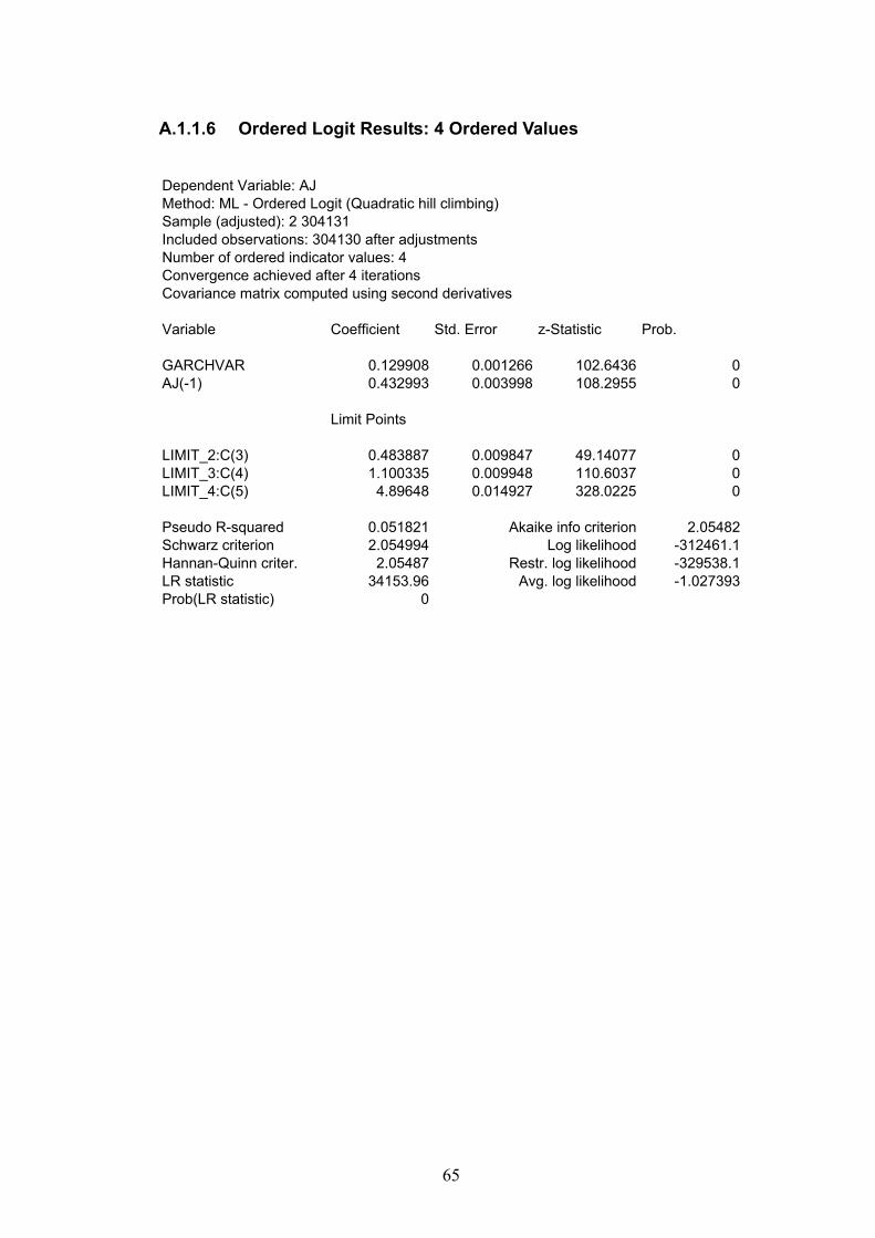
65
A.1.1.6 Ordered Logit Results: 4 Ordered Values
Dependent Variable: AJMethod: ML - Ordered Logit (Quadratic hill climbing)Sample (adjusted): 2 304131Included observations: 304130 after adjustmentsNumber of ordered indicator values: 4Convergence achieved after 4 iterationsCovariance matrix computed using second derivatives
Variable Coefficient Std. Error z-Statistic Prob.
GARCHVAR 0.129908 0.001266 102.6436 0AJ(-1) 0.432993 0.003998 108.2955 0
Limit Points
LIMIT_2:C(3) 0.483887 0.009847 49.14077 0LIMIT_3:C(4) 1.100335 0.009948 110.6037 0LIMIT_4:C(5) 4.89648 0.014927 328.0225 0
Pseudo R-squared 0.051821 Akaike info criterion 2.05482Schwarz criterion 2.054994 Log likelihood -312461.1Hannan-Quinn criter. 2.05487 Restr. log likelihood -329538.1LR statistic 34153.96 Avg. log likelihood -1.027393Prob(LR statistic) 0
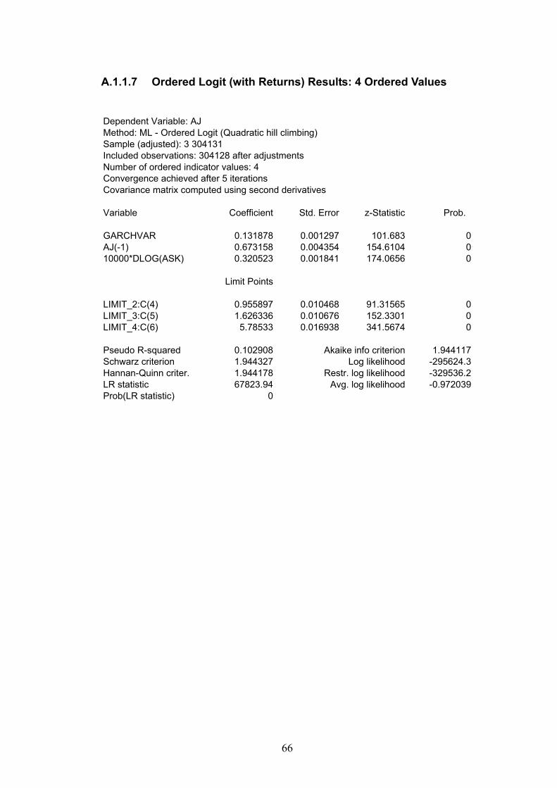
66
A.1.1.7 Ordered Logit (with Returns) Results: 4 Ordered Values
Dependent Variable: AJMethod: ML - Ordered Logit (Quadratic hill climbing)Sample (adjusted): 3 304131Included observations: 304128 after adjustmentsNumber of ordered indicator values: 4Convergence achieved after 5 iterationsCovariance matrix computed using second derivatives
Variable Coefficient Std. Error z-Statistic Prob.
GARCHVAR 0.131878 0.001297 101.683 0AJ(-1) 0.673158 0.004354 154.6104 010000*DLOG(ASK) 0.320523 0.001841 174.0656 0
Limit Points
LIMIT_2:C(4) 0.955897 0.010468 91.31565 0LIMIT_3:C(5) 1.626336 0.010676 152.3301 0LIMIT_4:C(6) 5.78533 0.016938 341.5674 0
Pseudo R-squared 0.102908 Akaike info criterion 1.944117Schwarz criterion 1.944327 Log likelihood -295624.3Hannan-Quinn criter. 1.944178 Restr. log likelihood -329536.2LR statistic 67823.94 Avg. log likelihood -0.972039Prob(LR statistic) 0

67
A.1.1.8 Ordered Logit Results: 10 Ordered Values
Dependent Variable: AJMethod: ML - Ordered Logit (Quadratic hill climbing)Sample (adjusted): 2 308749Included observations: 307943 after adjustmentsNumber of ordered indicator values: 10Convergence achieved after 7 iterationsCovariance matrix computed using second derivatives
Variable Coefficient Std. Error z-Statistic Prob.
GARCHVAR 0.155742 0.001351 115.2591 0AJ(-1) 0.159926 0.001594 100.3382 0
Limit Points
LIMIT_2:C(3) -5.137085 0.053891 -95.32363 0LIMIT_3:C(4) -3.762068 0.028652 -131.3013 0LIMIT_4:C(5) -3.158783 0.022402 -141.0075 0LIMIT_5:C(6) 0.717831 0.011771 60.98525 0LIMIT_6:C(7) 0.729267 0.011771 61.95536 0LIMIT_7:C(8) 1.29396 0.011879 108.9279 0LIMIT_8:C(9) 1.339747 0.011894 112.6399 0LIMIT_9:C(10) 1.341132 0.011895 112.7518 0LIMIT_10:C(11) 5.194799 0.016561 313.6803 0
Pseudo R-squared 0.04758 Akaike info criterion 2.23514Schwarz criterion 2.23552 Log likelihood -344136.9Hannan-Quinn criter. 2.23525 Restr. log likelihood -361329LR statistic 34384.2 Avg. log likelihood -1.117534Prob(LR statistic) 0
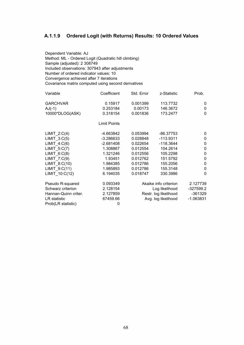
68
A.1.1.9 Ordered Logit (with Returns) Results: 10 Ordered Values
Dependent Variable: AJMethod: ML - Ordered Logit (Quadratic hill climbing)Sample (adjusted): 2 308749Included observations: 307943 after adjustmentsNumber of ordered indicator values: 10Convergence achieved after 7 iterationsCovariance matrix computed using second derivatives
Variable Coefficient Std. Error z-Statistic Prob.
GARCHVAR 0.15917 0.001399 113.7732 0AJ(-1) 0.253184 0.00173 146.3672 010000*DLOG(ASK) 0.318154 0.001836 173.2477 0
Limit Points
LIMIT_2:C(4) -4.663842 0.053994 -86.37753 0LIMIT_3:C(5) -3.286633 0.028848 -113.9311 0LIMIT_4:C(6) -2.681408 0.022654 -118.3644 0LIMIT_5:C(7) 1.308867 0.012554 104.2614 0LIMIT_6:C(8) 1.321246 0.012556 105.2298 0LIMIT_7:C(9) 1.93451 0.012762 151.5792 0LIMIT_8:C(10) 1.984385 0.012786 155.2056 0LIMIT_9:C(11) 1.985893 0.012786 155.3148 0LIMIT_10:C(12) 6.194035 0.018747 330.3986 0
Pseudo R-squared 0.093349 Akaike info criterion 2.127739Schwarz criterion 2.128154 Log likelihood -327599.2Hannan-Quinn criter. 2.127859 Restr. log likelihood -361329LR statistic 67459.66 Avg. log likelihood -1.063831Prob(LR statistic) 0

69
A.1.2 Dataset 2: USD-USD April 1989 to June 1989:
A.1.2.1 MA(1)-GARCH(1,1) Results:
Dependent Variable: 10000*DLOG(ASK)Method: ML - ARCHSample (adjusted): 2 8445Included observations: 8444 after adjustmentsConvergence achieved after 37 iterationsMA Backcast: 1Presample variance: backcast (parameter = 0.7)GARCH = C(3) + C(4)*RESID(-1)^2 + C(5)*GARCH(-1)
Variable Coefficient Std. Error z-Statistic Prob.
C 0.045205 0.013771 3.282516 0.001MA(1) -0.3281 0.011435 -28.693 0
Variance Equation
C 0.683349 0.025552 26.7437 0RESID(-1)^2 0.265029 0.008055 32.9008 0GARCH(-1) 0.653991 0.007513 87.05354 0
R-squared 0.046483 Mean dependent var 0.001809Adjusted R-squared 0.04637 S.D. dependent var 2.611027S.E. of regression 2.549771 Akaike info criterion 4.444882Sum squared resid 54884.24 Schwarz criterion 4.449051Log likelihood -18761.29 Hannan-Quinn criter. 4.446305Durbin-Watson stat 1.819609
Inverted MA Roots 0.33

70
A.1.2.2 Ordered Probit Results: 4 Ordered Values
Dependent Variable: AJMethod: ML - Ordered Probit (Quadratic hill climbing)Sample (adjusted): 2 8445Included observations: 8444 after adjustmentsNumber of ordered indicator values: 4Convergence achieved after 5 iterationsCovariance matrix computed using second derivatives
Variable Coefficient Std. Error z-Statistic Prob.
GARCH01 0.009127 0.000855 10.67187 0AJ(-1) 0.942999 0.042231 22.3298 0
Limit Points
LIMIT_2:C(3) 0.61897 0.123303 5.019921 0LIMIT_3:C(4) 1.002232 0.121611 8.241273 0LIMIT_4:C(5) 4.898957 0.134626 36.38941 0
Pseudo R-squared 0.115395 Akaike info criterion 0.581462Schwarz criterion 0.585632 Log likelihood -2449.933Hannan-Quinn criter. 0.582885 Restr. log likelihood -2769.524LR statistic 639.1806 Avg. log likelihood -0.290139Prob(LR statistic) 0

71
A.1.2.3 Ordered Probit (with Returns) Results: 4 Ordered Values
Dependent Variable: AJMethod: ML - Ordered Probit (Quadratic hill climbing)Sample (adjusted): 2 8445Included observations: 8444 after adjustmentsNumber of ordered indicator values: 4Convergence achieved after 5 iterationsCovariance matrix computed using second derivatives
Variable Coefficient Std. Error z-Statistic Prob.
GARCHVAR 0.00933 0.000852 10.94538 0AJ(-1) 1.008975 0.043056 23.43378 010000*DLOG(ASK) 0.08268 0.006736 12.27428 0
Limit Points
LIMIT_2:C(4) 0.775747 0.125149 6.198581 0LIMIT_3:C(5) 1.166192 0.12345 9.446642 0LIMIT_4:C(6) 5.148438 0.138288 37.22976 0
Pseudo R-squared 0.142475 Akaike info criterion 0.563936Schwarz criterion 0.568939 Log likelihood -2374.936Hannan-Quinn criter. 0.565644 Restr. log likelihood -2769.524LR statistic 789.1746 Avg. log likelihood -0.281257Prob(LR statistic) 0

72
A.1.2.4 Ordered Probit Results: 10 Ordered Values
Dependent Variable: AJMethod: ML - Ordered Probit (Quadratic hill climbing)Sample (adjusted): 2 8445Included observations: 8444 after adjustmentsNumber of ordered indicator values: 10Convergence achieved after 7 iterationsCovariance matrix computed using second derivatives
Variable Coefficient Std. Error z-Statistic Prob.
GARCHVAR 0.010588 0.000829 12.7664 0AJ(-1) 0.293255 0.018241 16.07658 0
Limit Points
LIMIT_2:C(3) -1.046148 0.251299 -4.162967 0LIMIT_3:C(4) -0.925167 0.225398 -4.104586 0LIMIT_4:C(5) -0.71307 0.195539 -3.646689 0.0003LIMIT_5:C(6) 0.463308 0.159031 2.91332 0.0036LIMIT_6:C(7) 0.525466 0.158821 3.308537 0.0009LIMIT_7:C(8) 0.77686 0.158252 4.908998 0LIMIT_8:C(9) 0.837742 0.158161 5.296765 0LIMIT_9:C(10) 0.843638 0.158153 5.334317 0LIMIT_10:C(11) 4.644992 0.167892 27.66655 0
Pseudo R-squared 0.069425 Akaike info criterion 0.65859Schwarz criterion 0.667763 Log likelihood -2769.568Hannan-Quinn criter. 0.661721 Restr. log likelihood -2976.191LR statistic 413.2452 Avg. log likelihood -0.327992Prob(LR statistic) 0
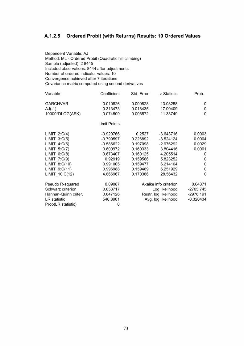
73
A.1.2.5 Ordered Probit (with Returns) Results: 10 Ordered Values
Dependent Variable: AJMethod: ML - Ordered Probit (Quadratic hill climbing)Sample (adjusted): 2 8445Included observations: 8444 after adjustmentsNumber of ordered indicator values: 10Convergence achieved after 7 iterationsCovariance matrix computed using second derivatives
Variable Coefficient Std. Error z-Statistic Prob.
GARCHVAR 0.010826 0.000828 13.08258 0AJ(-1) 0.313473 0.018435 17.00409 010000*DLOG(ASK) 0.074509 0.006572 11.33749 0
Limit Points
LIMIT_2:C(4) -0.920766 0.2527 -3.643716 0.0003LIMIT_3:C(5) -0.799597 0.226892 -3.524124 0.0004LIMIT_4:C(6) -0.586622 0.197098 -2.976292 0.0029LIMIT_5:C(7) 0.609972 0.160333 3.804416 0.0001LIMIT_6:C(8) 0.673407 0.160125 4.205514 0LIMIT_7:C(9) 0.92919 0.159566 5.823252 0LIMIT_8:C(10) 0.991005 0.159477 6.214104 0LIMIT_9:C(11) 0.996988 0.159469 6.251929 0LIMIT_10:C(12) 4.866967 0.170386 28.56432 0
Pseudo R-squared 0.09087 Akaike info criterion 0.64371Schwarz criterion 0.653717 Log likelihood -2705.745Hannan-Quinn criter. 0.647126 Restr. log likelihood -2976.191LR statistic 540.8901 Avg. log likelihood -0.320434Prob(LR statistic) 0

74
A.1.2.6 Ordered Logit Results: 4 Ordered Values
Dependent Variable: AJMethod: ML - Ordered Logit (Quadratic hill climbing)Sample (adjusted): 2 8445Included observations: 8444 after adjustmentsNumber of ordered indicator values: 4Convergence achieved after 7 iterationsCovariance matrix computed using second derivatives
Variable Coefficient Std. Error z-Statistic Prob.
GARCHVAR 0.023145 0.002506 9.234157 0AJ(-1) 1.816022 0.078415 23.15919 0
Limit Points
LIMIT_2:C(3) 1.151811 0.221143 5.208446 0LIMIT_3:C(4) 2.052707 0.215518 9.524505 0LIMIT_4:C(5) 9.285628 0.252771 36.73541 0
Pseudo R-squared 0.11296 Akaike info criterion 0.583059Schwarz criterion 0.587229 Log likelihood -2456.677Hannan-Quinn criter. 0.584483 Restr. log likelihood -2769.524LR statistic 625.6929 Avg. log likelihood -0.290938Prob(LR statistic) 0

75
A.1.2.7 Ordered Logit (with Returns) Results: 4 Ordered Values
Dependent Variable: AJMethod: ML - Ordered Logit (Quadratic hill climbing)Sample (adjusted): 2 8445Included observations: 8444 after adjustmentsNumber of ordered indicator values: 4Convergence achieved after 8 iterationsCovariance matrix computed using second derivatives
Variable Coefficient Std. Error z-Statistic Prob.
GARCHVAR 0.023498 0.002679 8.772378 0AJ(-1) 1.937969 0.080338 24.12276 010000*DLOG(ASK) 0.179594 0.014658 12.25201 0
Limit Points
LIMIT_2:C(4) 1.431605 0.224685 6.371611 0LIMIT_3:C(5) 2.341427 0.219477 10.66822 0LIMIT_4:C(6) 9.770045 0.261472 37.36562 0
Pseudo R-squared 0.139367 Akaike info criterion 0.565974Schwarz criterion 0.570977 Log likelihood -2383.542Hannan-Quinn criter. 0.567682 Restr. log likelihood -2769.524LR statistic 771.9628 Avg. log likelihood -0.282276Prob(LR statistic) 0

76
A.1.2.8 Ordered Logit Results: 10 Ordered Values
Dependent Variable: AJMethod: ML - Ordered Logit (Quadratic hill climbing)Sample (adjusted): 2 8445Included observations: 8444 after adjustmentsNumber of ordered indicator values: 10Convergence achieved after 6 iterationsCovariance matrix computed using second derivatives
Variable Coefficient Std. Error z-Statistic Prob.
GARCHVAR 0.030535 0.00282 10.82827 0AJ(-1) 0.563651 0.033692 16.72951 0
Limit Points
LIMIT_2:C(3) -3.399721 0.756259 -4.495444 0LIMIT_3:C(4) -2.993661 0.63663 -4.702359 0LIMIT_4:C(5) -2.298438 0.488651 -4.703637 0LIMIT_5:C(6) 0.926596 0.286528 3.233876 0.0012LIMIT_6:C(7) 1.076884 0.285436 3.77277 0.0002LIMIT_7:C(8) 1.66173 0.282811 5.875773 0LIMIT_8:C(9) 1.797737 0.282485 6.364009 0LIMIT_9:C(10) 1.810792 0.282458 6.41083 0LIMIT_10:C(11) 8.845043 0.310773 28.46145 0
Pseudo R-squared 0.068507 Akaike info criterion 0.659237Schwarz criterion 0.66841 Log likelihood -2772.3Hannan-Quinn criter. 0.662368 Restr. log likelihood -2976.191LR statistic 407.7821 Avg. log likelihood -0.328316Prob(LR statistic) 0

77
A.1.2.9 Ordered Logit (with Returns) Results: 10 Ordered Values
Dependent Variable: AJMethod: ML - Ordered Logit (Quadratic hill climbing)Sample (adjusted): 2 8445Included observations: 8444 after adjustmentsNumber of ordered indicator values: 10Convergence achieved after 8 iterationsCovariance matrix computed using second derivatives
Variable Coefficient Std. Error z-Statistic Prob.
GARCHVAR 0.031698 0.002984 10.62409 0AJ(-1) 0.605872 0.03419 17.72067 010000*DLOG(ASK) 0.167709 0.014728 11.38731 0
Limit Points
LIMIT_2:C(4) -3.108606 0.756454 -4.109446 0LIMIT_3:C(5) -2.702375 0.63687 -4.243211 0LIMIT_4:C(6) -2.004677 0.48917 -4.098116 0LIMIT_5:C(7) 1.236004 0.289368 4.271391 0LIMIT_6:C(8) 1.387414 0.288368 4.811259 0LIMIT_7:C(9) 1.976024 0.286018 6.908731 0LIMIT_8:C(10) 2.112879 0.285744 7.394317 0LIMIT_9:C(11) 2.126018 0.285722 7.440867 0LIMIT_10:C(12) 9.336144 0.318108 29.349 0
Pseudo R-squared 0.09058 Akaike info criterion 0.643914Schwarz criterion 0.653921 Log likelihood -2706.607Hannan-Quinn criter. 0.64733 Restr. log likelihood -2976.191LR statistic 539.1676 Avg. log likelihood -0.320536Prob(LR statistic) 0

78
A.1.3 Dataset 3: USD-USD April 2006 to May 2006:
A.1.3.1 MA(1)-GARCH(1,1) Results:
Dependent Variable: 10000*DLOG(ASK)Method: ML - ARCH (Marquardt) - Normal distributionSample (adjusted): 2 551356Included observations: 551355 after adjustmentsConvergence achieved after 14 iterationsMA Backcast: 1Presample variance: backcast (parameter = 0.7)GARCH = C(3) + C(4)*RESID(-1)^2 + C(5)*GARCH(-1)
Variable Coefficient Std. Error z-Statistic Prob.
C 0.002535 0.000358 7.075531 0MA(1) -0.781719 0.000858 -911.204 0
Variance Equation
C 0.057826 0.000813 71.15628 0RESID(-1)^2 0.063219 0.000558 113.2785 0GARCH(-1) 0.902484 0.000889 1015.04 0
R-squared 0.372225 Mean dependent var -0.000425Adjusted R-squared 0.372224 S.D. dependent var 1.657286S.E. of regression 1.313106 Akaike info criterion 3.302185Sum squared resid 950669.3 Schwarz criterion 3.302287Log likelihood -910333.2 Hannan-Quinn criter. 3.302214Durbin-Watson stat 1.97678
Inverted MA Roots 0.78

79
A.1.3.2 Ordered Probit Results: 4 Ordered Values
Dependent Variable: AJMethod: ML - Ordered Probit (Quadratic hill climbing)Sample (adjusted): 2 551356Included observations: 551355 after adjustmentsNumber of ordered indicator values: 4Convergence achieved after 4 iterationsCovariance matrix computed using second derivatives
Variable Coefficient Std. Error z-Statistic Prob.
GARCHVAR 0.046421 0.001588 29.24124 0AJ(-1) -0.130554 0.001879 -69.46221 0
Limit Points
LIMIT_2:C(3) -0.267391 0.004557 -58.67524 0LIMIT_3:C(4) 0.497267 0.004577 108.652 0LIMIT_4:C(5) 3.624999 0.036661 98.87791 0
Pseudo R-squared 0.00466 Akaike info criterion 2.122714Schwarz criterion 2.122815 Log likelihood -585179.4Hannan-Quinn criter. 2.122742 Restr. log likelihood -587919.3LR statistic 5479.851 Avg. log likelihood -1.061348Prob(LR statistic) 0

80
A.1.3.3 Ordered Probit (with Returns) Results: 4 Ordered Values
Dependent Variable: AJMethod: ML - Ordered Probit (Quadratic hill climbing)Sample (adjusted): 2 551356Included observations: 551355 after adjustmentsNumber of ordered indicator values: 4Convergence achieved after 6 iterationsCovariance matrix computed using second derivatives
Variable Coefficient Std. Error z-Statistic Prob.
GARCHVAR 0.032475 0.001698 19.12882 0AJ(-1) 0.520271 0.002468 210.7702 010000*DLOG(ASK) 0.624067 0.001388 449.5486 0
Limit Points
LIMIT_2:C(4) 0.803072 0.005446 147.4683 0LIMIT_3:C(5) 1.84724 0.00582 317.4066 0LIMIT_4:C(6) 6.264271 0.051481 121.682 0
Pseudo R-squared 0.202812 Akaike info criterion 1.700133Schwarz criterion 1.700255 Log likelihood -468682.4Hannan-Quinn criter. 1.700167 Restr. log likelihood -587919.3LR statistic 238473.8 Avg. log likelihood -0.850056Prob(LR statistic) 0

81
A.1.3.4 Ordered Probit Results: 10 Ordered Values
Dependent Variable: AJMethod: ML - Ordered Probit (Quadratic hill climbing)Sample (adjusted): 2 551356Included observations: 530382 after adjustmentsNumber of ordered indicator values: 10Convergence achieved after 5 iterationsCovariance matrix computed using second derivatives
Variable Coefficient Std. Error z-Statistic Prob.
GARCHVAR 0.029623 0.001543 19.20169 0AJ(-1) -0.040361 0.000655 -61.5938 0
Limit Points
LIMIT_2:C(3) -2.770052 0.008137 -340.4275 0LIMIT_3:C(4) -2.123895 0.005776 -367.693 0LIMIT_4:C(5) -1.541017 0.005154 -299.0033 0LIMIT_5:C(6) -0.292156 0.004841 -60.34619 0LIMIT_6:C(7) -0.076775 0.004831 -15.89255 0LIMIT_7:C(8) 0.218854 0.004827 45.33503 0LIMIT_8:C(9) 0.463249 0.00484 95.70278 0LIMIT_9:C(10) 0.472672 0.004841 97.63469 0LIMIT_10:C(11) 3.593189 0.037289 96.36043 0
Pseudo R-squared 0.00228 Akaike info criterion 3.351617Schwarz criterion 3.351849 Log likelihood -888807.6Hannan-Quinn criter. 3.351682 Restr. log likelihood -890838.9LR statistic 4062.696 Avg. log likelihood -1.675788Prob(LR statistic) 0

82
A.1.3.5 Ordered Probit (with Returns) Results: 10 Ordered Values
Dependent Variable: AJMethod: ML - Ordered Probit (Quadratic hill climbing)Sample (adjusted): 2 551356Included observations: 530382 after adjustmentsNumber of ordered indicator values: 10Failure to improve Likelihood after 17 iterationsCovariance matrix computed using second derivatives
Variable Coefficient Std. Error z-Statistic Prob.
GARCHVAR -0.035043 0.001544 -22.69168 0AJ(-1) 0.01852 0.000821 22.56212 010000*DLOG(ASK) 0.365238 0.001223 298.6273 0
Limit Points
LIMIT_2:C(4) -2.768453 0.008501 -325.6782 0LIMIT_3:C(5) -2.089688 0.006173 -338.5115 0LIMIT_4:C(6) -1.484632 0.00565 -262.7437 0LIMIT_5:C(7) -0.148442 0.005549 -26.74997 0LIMIT_6:C(8) 0.084178 0.005598 15.03649 0LIMIT_7:C(9) 0.395925 0.005688 69.60886 0LIMIT_8:C(10) 0.648621 0.005789 112.0419 0LIMIT_9:C(11) 0.659757 0.005795 113.8488 0LIMIT_10:C(12) 4.041679 0.025918 155.9393 0
Pseudo R-squared 0.101511 Akaike info criterion 3.018282Schwarz criterion 3.018535 Log likelihood -800409.1Hannan-Quinn criter. 3.018353 Restr. log likelihood -890838.9LR statistic 180859.6 Avg. log likelihood -1.509118Prob(LR statistic) 0

83
A.1.3.6 Ordered Logit Results: 4 Ordered Values
Dependent Variable: AJMethod: ML - Ordered Logit (Quadratic hill climbing)Sample (adjusted): 2 551356Included observations: 551355 after adjustmentsNumber of ordered indicator values: 4Convergence achieved after 4 iterationsCovariance matrix computed using second derivatives
Variable Coefficient Std. Error z-Statistic Prob.
GARCHVAR 0.080152 0.00277 28.93061 0AJ(-1) -0.204018 0.003055 -66.79117 0
Limit Points
LIMIT_2:C(3) -0.41091 0.007581 -54.20336 0LIMIT_3:C(4) 0.830244 0.007658 108.4198 0LIMIT_4:C(5) 9.135262 0.144521 63.21045 0
Pseudo R-squared 0.004388 Akaike info criterion 2.123295Schwarz criterion 2.123397 Log likelihood -585339.7Hannan-Quinn criter. 2.123324 Restr. log likelihood -587919.3LR statistic 5159.321 Avg. log likelihood -1.061638Prob(LR statistic) 0

84
A.1.3.7 Ordered Logit (with Returns) Results: 4 Ordered Values
Dependent Variable: AJMethod: ML - Ordered Logit (Quadratic hill climbing)Sample (adjusted): 2 551356Included observations: 551355 after adjustmentsNumber of ordered indicator values: 4Convergence achieved after 6 iterationsCovariance matrix computed using second derivatives
Variable Coefficient Std. Error z-Statistic Prob.
GARCHVAR 0.048475 0.003264 14.85304 0AJ(-1) 1.053246 0.004586 229.6602 010000*DLOG(ASK) 1.215211 0.002966 409.7483 0
Limit Points
LIMIT_2:C(4) 1.600267 0.009958 160.7016 0LIMIT_3:C(5) 3.453473 0.011048 312.5789 0LIMIT_4:C(6) 13.6294 0.167398 81.41909 0
Pseudo R-squared 0.216154 Akaike info criterion 1.671678Schwarz criterion 1.671801 Log likelihood -460838.1Hannan-Quinn criter. 1.671713 Restr. log likelihood -587919.3LR statistic 254162.3 Avg. log likelihood -0.835828Prob(LR statistic) 0

85
A.1.3.8 Ordered Logit Results: 10 Ordered Values
Dependent Variable: AJMethod: ML - Ordered Logit (Quadratic hill climbing)Sample (adjusted): 2 551356Included observations: 530382 after adjustmentsNumber of ordered indicator values: 10Convergence achieved after 5 iterationsCovariance matrix computed using second derivatives
Variable Coefficient Std. Error z-Statistic Prob.
GARCHVAR 0.059869 0.002706 22.12459 0AJ(-1) -0.07549 0.001114 -67.78632 0
Limit Points
LIMIT_2:C(3) -5.681481 0.021378 -265.7677 0LIMIT_3:C(4) -3.965107 0.011679 -339.4939 0LIMIT_4:C(5) -2.690845 0.009268 -290.3316 0LIMIT_5:C(6) -0.512979 0.008257 -62.12349 0LIMIT_6:C(7) -0.168038 0.008229 -20.41918 0LIMIT_7:C(8) 0.3095 0.008227 37.61812 0LIMIT_8:C(9) 0.714603 0.008278 86.32978 0LIMIT_9:C(10) 0.73051 0.008281 88.22038 0LIMIT_10:C(11) 9.036028 0.147643 61.20197 0
Pseudo R-squared 0.0028 Akaike info criterion 3.34987Schwarz criterion 3.350102 Log likelihood -888344.5Hannan-Quinn criter. 3.349936 Restr. log likelihood -890838.9LR statistic 4988.841 Avg. log likelihood -1.674915Prob(LR statistic) 0

86
A.1.3.9 Ordered Logit (with Returns) Results: 10 Ordered Values
Dependent Variable: AJMethod: ML - Ordered Logit (Quadratic hill climbing)Sample (adjusted): 2 551356Included observations: 530382 after adjustmentsNumber of ordered indicator values: 10Convergence achieved after 6 iterationsCovariance matrix computed using second derivatives
Variable Coefficient Std. Error z-Statistic Prob.
GARCHVAR 0.067262 0.003175 21.18593 0AJ(-1) 0.402995 0.0016 251.9007 010000*DLOG(ASK) 1.189108 0.002737 434.4841 0
Limit Points
LIMIT_2:C(4) -3.894364 0.022026 -176.8036 0LIMIT_3:C(5) -2.114505 0.012808 -165.0968 0LIMIT_4:C(6) -0.7165 0.010767 -66.54475 0LIMIT_5:C(7) 2.04924 0.010738 190.8341 0LIMIT_6:C(8) 2.528082 0.010914 231.6353 0LIMIT_7:C(9) 3.225475 0.011271 286.1774 0LIMIT_8:C(10) 3.846774 0.011692 329.0122 0LIMIT_9:C(11) 3.872262 0.011712 330.6322 0LIMIT_10:C(12) 13.94908 0.170499 81.81305 0
Pseudo R-squared 0.146499 Akaike info criterion 2.867156Schwarz criterion 2.867409 Log likelihood -760331.9Hannan-Quinn criter. 2.867227 Restr. log likelihood -890838.9LR statistic 261014.1 Avg. log likelihood -1.433555Prob(LR statistic) 0
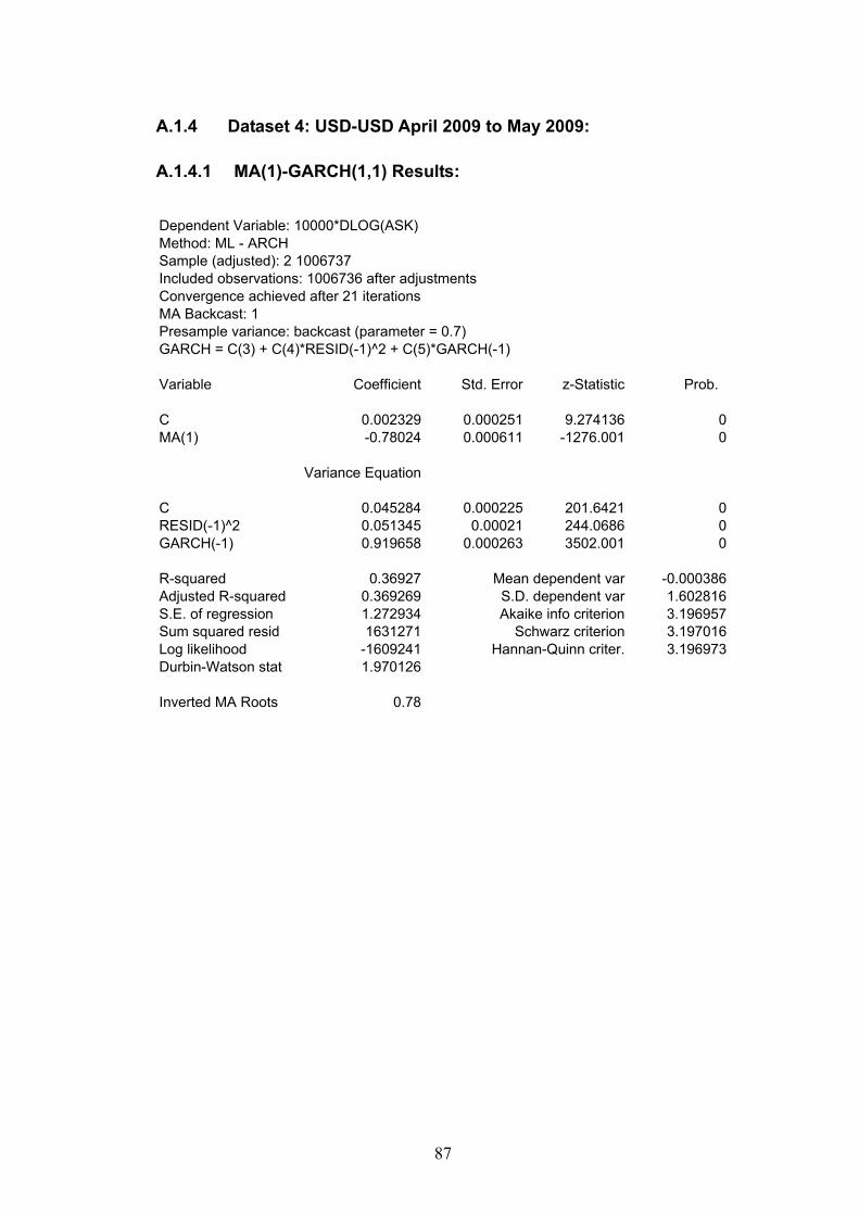
87
A.1.4 Dataset 4: USD-USD April 2009 to May 2009:
A.1.4.1 MA(1)-GARCH(1,1) Results:
Dependent Variable: 10000*DLOG(ASK)Method: ML - ARCHSample (adjusted): 2 1006737Included observations: 1006736 after adjustmentsConvergence achieved after 21 iterationsMA Backcast: 1Presample variance: backcast (parameter = 0.7)GARCH = C(3) + C(4)*RESID(-1)^2 + C(5)*GARCH(-1)
Variable Coefficient Std. Error z-Statistic Prob.
C 0.002329 0.000251 9.274136 0MA(1) -0.78024 0.000611 -1276.001 0
Variance Equation
C 0.045284 0.000225 201.6421 0RESID(-1)^2 0.051345 0.00021 244.0686 0GARCH(-1) 0.919658 0.000263 3502.001 0
R-squared 0.36927 Mean dependent var -0.000386Adjusted R-squared 0.369269 S.D. dependent var 1.602816S.E. of regression 1.272934 Akaike info criterion 3.196957Sum squared resid 1631271 Schwarz criterion 3.197016Log likelihood -1609241 Hannan-Quinn criter. 3.196973Durbin-Watson stat 1.970126
Inverted MA Roots 0.78

88
A.1.4.2 Ordered Probit Results: 4 Ordered Values
Dependent Variable: AJMethod: ML - Ordered Probit (Quadratic hill climbing)Sample (adjusted): 2 1006737Included observations: 1006736 after adjustmentsNumber of ordered indicator values: 4Convergence achieved after 3 iterationsCovariance matrix computed using second derivatives
Variable Coefficient Std. Error z-Statistic Prob.
GARCHVAR 0.098754 0.000867 113.8863 0AJ(-1) 0.262245 0.00148 177.1729 0
Limit Points
LIMIT_2:C(3) 0.300383 0.003019 99.50314 0LIMIT_3:C(4) 1.797373 0.003373 532.8891 0LIMIT_4:C(5) 2.392075 0.003801 629.366 0
Pseudo R-squared 0.024794 Akaike info criterion 2.069774Schwarz criterion 2.069833 Log likelihood -1041853Hannan-Quinn criter. 2.069791 Restr. log likelihood -1068342LR statistic 52977.45 Avg. log likelihood -1.034882Prob(LR statistic) 0

89
A.1.4.3 Ordered Probit (with Returns) Results: 4 Ordered Values
Dependent Variable: AJMethod: ML - Ordered Probit (Quadratic hill climbing)Sample (adjusted): 2 1006737Included observations: 1006736 after adjustmentsNumber of ordered indicator values: 4Convergence achieved after 12 iterationsCovariance matrix computed using second derivatives
Variable Coefficient Std. Error z-Statistic Prob.
GARCHVAR 0.040619 0.000907 44.7718 0AJ(-1) 0.260624 0.001785 146.0215 010000*DLOG(ASK) 0.415817 0.00095 437.6876 0
Limit Points
LIMIT_2:C(4) 0.072632 0.003441 21.10602 0LIMIT_3:C(5) 1.741812 0.004059 429.1621 0LIMIT_4:C(6) 2.420409 0.004675 517.7516 0
Pseudo R-squared 0.176356 Akaike info criterion 1.748103Schwarz criterion 1.748173 Log likelihood -879933.1Hannan-Quinn criter. 1.748122 Restr. log likelihood -1068342LR statistic 376817.7 Avg. log likelihood -0.874046Prob(LR statistic) 0

90
A.1.4.4 Ordered Probit Results: 10 Ordered Values
Dependent Variable: AJMethod: ML - Ordered Probit (Quadratic hill climbing)Sample (adjusted): 2 1006737Included observations: 1006736 after adjustmentsNumber of ordered indicator values: 10Convergence achieved after 4 iterationsCovariance matrix computed using second derivatives
Variable Coefficient Std. Error z-Statistic Prob.
GARCHVAR 0.096416 0.000823 117.0911 0AJ(-1) 0.088372 0.000415 212.8967 0
Limit Points
LIMIT_2:C(3) -1.466867 0.003573 -410.4852 0LIMIT_3:C(4) -0.169471 0.002717 -62.38151 0LIMIT_4:C(5) 0.142757 0.00271 52.67088 0LIMIT_5:C(6) 0.32063 0.002718 117.9753 0LIMIT_6:C(7) 0.463947 0.002729 170.0266 0LIMIT_7:C(8) 0.855945 0.002774 308.5626 0LIMIT_8:C(9) 1.630826 0.002965 549.9868 0LIMIT_9:C(10) 1.799457 0.003034 593.0574 0LIMIT_10:C(11) 2.394888 0.003495 685.2099 0
Pseudo R-squared 0.016257 Akaike info criterion 4.058805Schwarz criterion 4.058934 Log likelihood -2043062Hannan-Quinn criter. 4.05884 Restr. log likelihood -2076824LR statistic 67525.47 Avg. log likelihood -2.029392Prob(LR statistic) 0

91
A.1.4.5 Ordered Probit (with Returns) Results: 10 Ordered Values
Dependent Variable: AJMethod: ML - Ordered Probit (Quadratic hill climbing)Sample (adjusted): 2 1006737Included observations: 1006736 after adjustmentsNumber of ordered indicator values: 10Convergence achieved after 9 iterationsCovariance matrix computed using second derivatives
Variable Coefficient Std. Error z-Statistic Prob.
GARCHVAR -0.003187 0.000829 -3.843887 0.0001AJ(-1) 0.094896 0.000502 188.9157 010000*DLOG(ASK) 0.399614 0.000853 468.5108 0
Limit Points
LIMIT_2:C(4) -1.889585 0.00377 -501.2568 0LIMIT_3:C(5) -0.540899 0.002964 -182.4773 0LIMIT_4:C(6) -0.211211 0.003013 -70.09902 0LIMIT_5:C(7) -0.014555 0.003062 -4.753915 0LIMIT_6:C(8) 0.153294 0.003113 49.24206 0LIMIT_7:C(9) 0.615502 0.003255 189.0877 0LIMIT_8:C(10) 1.481455 0.003579 413.8783 0LIMIT_9:C(11) 1.676514 0.003697 453.4845 0LIMIT_10:C(12) 2.40264 0.004378 548.8559 0
Pseudo R-squared 0.096012 Akaike info criterion 3.729748Schwarz criterion 3.729889 Log likelihood -1877424Hannan-Quinn criter. 3.729787 Restr. log likelihood -2076824LR statistic 398801.1 Avg. log likelihood -1.864862Prob(LR statistic) 0

92
A.1.4.6 Ordered Logit Results: 4 Ordered Values
Dependent Variable: AJMethod: ML - Ordered Logit (Quadratic hill climbing)Sample (adjusted): 2 1006737Included observations: 1006736 after adjustmentsNumber of ordered indicator values: 4Convergence achieved after 4 iterationsCovariance matrix computed using second derivatives
Variable Coefficient Std. Error z-Statistic Prob.
GARCHVAR 0.214626 0.001959 109.574 0AJ(-1) 0.43948 0.002593 169.4684 0
Limit Points
LIMIT_2:C(3) 0.593662 0.00533 111.3912 0LIMIT_3:C(4) 3.114943 0.006332 491.9238 0LIMIT_4:C(5) 4.301442 0.007555 569.3761 0
Pseudo R-squared 0.024601 Akaike info criterion 2.070184Schwarz criterion 2.070243 Log likelihood -1042059Hannan-Quinn criter. 2.0702 Restr. log likelihood -1068342LR statistic 52565.01 Avg. log likelihood -1.035087Prob(LR statistic) 0

93
A.1.4.7 Ordered Logit (with Returns) Results: 4 Ordered Values
Dependent Variable: AJMethod: ML - Ordered Logit (Quadratic hill climbing)Sample (adjusted): 2 1006737Included observations: 1006736 after adjustmentsNumber of ordered indicator values: 4Convergence achieved after 5 iterationsCovariance matrix computed using second derivatives
Variable Coefficient Std. Error z-Statistic Prob.
GARCHVAR 0.222491 0.002315 96.11273 0AJ(-1) 1.964362 0.003971 494.6543 010000*DLOG(ASK) 1.38648 0.002369 585.1713 0
Limit Points
LIMIT_2:C(4) 2.992082 0.007366 406.2264 0LIMIT_3:C(5) 6.796605 0.010304 659.6204 0LIMIT_4:C(6) 8.504201 0.012206 696.7327 0
Pseudo R-squared 0.27793 Akaike info criterion 1.532523Schwarz criterion 1.532594 Log likelihood -771417.2Hannan-Quinn criter. 1.532543 Restr. log likelihood -1068342LR statistic 593849.5 Avg. log likelihood -0.766256Prob(LR statistic) 0
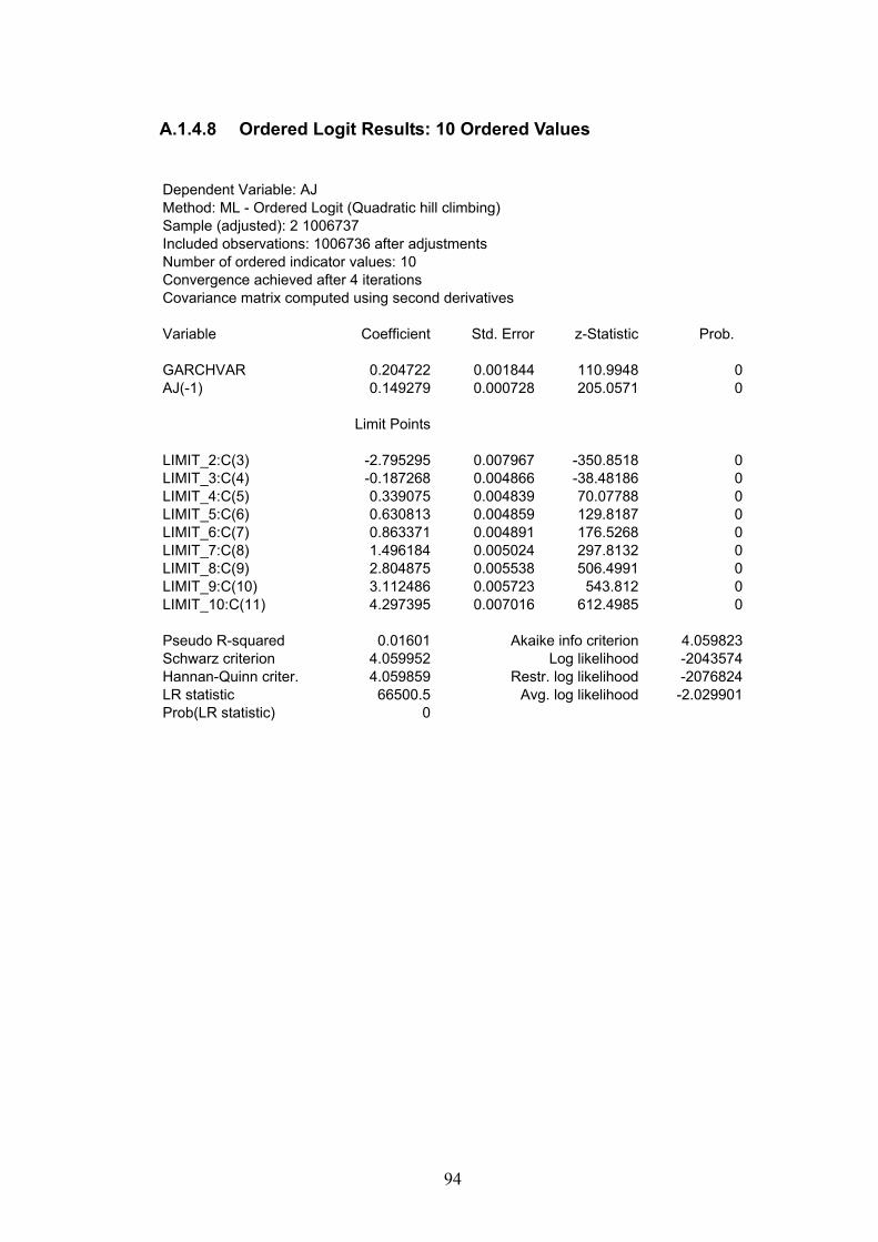
94
A.1.4.8 Ordered Logit Results: 10 Ordered Values
Dependent Variable: AJMethod: ML - Ordered Logit (Quadratic hill climbing)Sample (adjusted): 2 1006737Included observations: 1006736 after adjustmentsNumber of ordered indicator values: 10Convergence achieved after 4 iterationsCovariance matrix computed using second derivatives
Variable Coefficient Std. Error z-Statistic Prob.
GARCHVAR 0.204722 0.001844 110.9948 0AJ(-1) 0.149279 0.000728 205.0571 0
Limit Points
LIMIT_2:C(3) -2.795295 0.007967 -350.8518 0LIMIT_3:C(4) -0.187268 0.004866 -38.48186 0LIMIT_4:C(5) 0.339075 0.004839 70.07788 0LIMIT_5:C(6) 0.630813 0.004859 129.8187 0LIMIT_6:C(7) 0.863371 0.004891 176.5268 0LIMIT_7:C(8) 1.496184 0.005024 297.8132 0LIMIT_8:C(9) 2.804875 0.005538 506.4991 0LIMIT_9:C(10) 3.112486 0.005723 543.812 0LIMIT_10:C(11) 4.297395 0.007016 612.4985 0
Pseudo R-squared 0.01601 Akaike info criterion 4.059823Schwarz criterion 4.059952 Log likelihood -2043574Hannan-Quinn criter. 4.059859 Restr. log likelihood -2076824LR statistic 66500.5 Avg. log likelihood -2.029901Prob(LR statistic) 0

95
A.1.4.9 Ordered Logit (with Returns) Results: 10 Ordered Values
Dependent Variable: AJMethod: ML - Ordered Logit (Quadratic hill climbing)Sample (adjusted): 2 1006737Included observations: 1006736 after adjustmentsNumber of ordered indicator values: 10Convergence achieved after 5 iterationsCovariance matrix computed using second derivatives
Variable Coefficient Std. Error z-Statistic Prob.
GARCHVAR 0.268841 0.002158 124.5891 0AJ(-1) 0.575528 0.001002 574.3314 010000*DLOG(ASK) 1.283457 0.001961 654.4871 0
Limit Points
LIMIT_2:C(4) -1.499334 0.008444 -177.5703 0LIMIT_3:C(5) 1.549476 0.005795 267.3935 0LIMIT_4:C(6) 2.288018 0.005979 382.6506 0LIMIT_5:C(7) 2.734323 0.006163 443.6451 0LIMIT_6:C(8) 3.100859 0.006343 488.8769 0LIMIT_7:C(9) 4.034615 0.006789 594.2899 0LIMIT_8:C(10) 5.85286 0.007889 741.9462 0LIMIT_9:C(11) 6.285226 0.008209 765.6376 0LIMIT_10:C(12) 7.959922 0.010167 782.9249 0
Pseudo R-squared 0.158021 Akaike info criterion 3.473909Schwarz criterion 3.47405 Log likelihood -1748643Hannan-Quinn criter. 3.473948 Restr. log likelihood -2076824LR statistic 656363.1 Avg. log likelihood -1.736943Prob(LR statistic) 0