ANALYSIS OF RAIL RATES FOR WHEAT RAIL TRANSPORTATION IN MONTANA;

COMPARING RATES IN A CAPTIVE MARKET TO ONE WITH MORE INTRAMODAL COMPETITION

by

MATTHEW MCKAMEY

B.S., MONTANA STATE UNIVERSITY, 1999

A THESIS

Submitted in partial fulfillment of the

requirements for the degree

MASTER OF AGRIBUSINESS

Department of Agricultural Economics

College of Agriculture

KANSAS STATE UNIVERSITY

Manhattan, Kansas

2009

Approved by:

Major Professor DR. MICHAEL W. BABCOCK, Ph D.

ABSTRACT Today’s rail industry is the outcome of years of regulatory and technological

change. Since the passage of the Staggers Rail Act of 1980 the industry has seen

consolidation through mergers and acquisitions.

The rail industry in Montana has a rich rail history that includes the

completion of a northern east-west route over 100 years ago that provided a

commerce route from the interior of the US heartland to the ocean ports in the

Pacific Northwest. In those hundred years the rail traffic across Montana has seen

dramatic change. In the past, those routes have provided access for Montana

freight; today those routes primarily serve the needs of consumers and industries

far beyond Montana.

While the state’s economy is primarily agricultural, the largest user of rail

transportation is the energy industry. This leaves the agriculture industry with a

lower priority for access, providing a quandary for rail service for the grain industry

in the state.

In a state where more than eight national and regional rail carriers once

operated, Montana is now only serviced by a small handful, one of which operates

over 80% of the rail miles within its borders. Furthermore that carrier provides

service through those regions that are almost strictly agricultural, needing the

greatest access to the most cost effective means of transportation for the bulk

movement of grain.

The objectives of this thesis are to develop a model to measure railroad

costs and competition; determine the principal cost determinants and measure

intramodal competition by comparing the rates in a captive market (Montana) to

one with more intramodal competition (Kansas).

iv

TABLE OF CONTENTS

LIST OF TABLES ................................................................................................................. V 

LIST OF FIGURES ............................................................................................................. VI 

ACKNOWLEDGMENTS .................................................................................................. VII 

CHAPTER 1: INTRODUCTION .......................................................................................... 1 

1.1 Thesis Statement ...................................................................................................... 7 

1.2 Organization ............................................................................................................... 7 

CHAPTER 2: LITERATURE REVIEW .............................................................................. 8 

CHAPTER 3: THEORY ...................................................................................................... 16 

3.1 Railroad Reform Rationale .................................................................................... 16 

3.2 Perfect Competition ................................................................................................ 17 

3.3 Monopoly .................................................................................................................. 18 

3.4 Oligopoly ................................................................................................................... 18 

3.5 Intermodal Transportation System Theory ........................................................ 19 

3.6 Theoretical Model ................................................................................................... 20 

CHAPTER 4: EMPIRICAL MODEL ................................................................................. 22 

CHAPTER 5: DATA AND EMPIRICAL RESULTS ...................................................... 26 

5.1 Data ........................................................................................................................... 26 

5.2 Empirical Results .................................................................................................... 28 

CHAPTER 6: CONCLUSION ............................................................................................ 30 

REFERENCES ..................................................................................................................... 31 

v

LIST OF TABLES TABLE 1.1: RAILROADS OPERATING IN MONTANA, 2008 ................................... 3

TABLE 1.2: MONTANA WHEAT PRODUCTION 2003 – 2007 .................................. 6

TABLE 5.1: MONTANA AND KANSAS TRUCK MILES FROM ORIGINS ........... 26

TABLE 5.2: MEAN AND STANDARD DEVIATION OF VARIABLES .................... 27

TABLE 5.3: MONTANA AND KANSAS RAIL MILES FROM ORIGINS ................ 28

TABLE 5.4: RAILROAD RATE REGRESSION EQUATION ..................................... 29

vi

LIST OF FIGURES FIGURE 1.1: MONTANA RAIL MAP, 2008 ..................................................................... 5 

FIGURE 3.1: HYPOTHETICAL TRIP COST CURVES FOR RAIL (RR’), TRUCK (TT’), AND WATER (WW’), MODES OF TRANSPORTATION FOR A GIVEN ORIGIN/DESTINATION ..................................................................................................... 20 

FIGURE 4.1: METHOD FOR CALCULATION FOR BNSF RATES PER CWT-MILE ....................................................................................................................................... 23 

vii

ACKNOWLEDGMENTS

I wish to acknowledge several individuals who supported my efforts in

completing this thesis.

I wish to thank my parents, Les and Wendy McKamey, for their

encouragement and example to further pursue education and continually be a

student of learning. Thank you to my “in-laws”, Dan and Sandra DeBuff for

providing additional support, ideas and discussing the rail industry in Montana.

Thanks to my classmates within the MAB program for giving me the

opportunity to associate with and learn from their experiences and knowledge. I

would like to specifically thank Alex Offerdahl and Keith Kennedy for their

encouragement and example in completing my thesis.

I would like to thank the MAB Faculty and Staff for providing an opportunity

to pursue such an endeavor and for their patience and willingness to assist me in

completing the program. Thanks to Dr. Michael Babcock for his knowledge,

feedback, patience and tireless efforts he dedicated to my thesis.

Thanks to my children, Carson, Jackson and Mattison for their

understanding that allowed me the time to work at the computer uninterrupted.

Finally, and most importantly, I wish to express gratitude for my wife, Cindy,

for her never ending patience and careful reminders encouraging me to

accomplish my Masters Degree goal. Without her support and “forced” study time,

this project would have never been a reality.

1

CHAPTER 1: INTRODUCTION

Railroads are important for shipping agricultural commodities from producing

regions to the domestic processing locations and export ports. These shipments

typically involve large scale movements of a bulk commodity over long distances,

markets in which railroads have a cost advantage relative to other modes. This is

the situation in Montana where 70% of the Montana wheat crop is shipped by rail

to Portland and Seattle for export.

Railroads were the most heavily regulated transportation mode prior the

passage of the Staggers Rail Act in 1980. Deregulation gave the railroads a great

deal of pricing flexibility that was previously unavailable. Prices could be set as

low as variable cost and as high as 180% of variable cost without Interstate

Commerce Commission (ICC) jurisdiction or review. The Staggers Act set time

limits for ICC decisions regarding abandonments and mergers. Thus Class I

railroads were able to quickly abandon or sell branchlines that lost money.

Mergers reduced the number of Class I railroads from 40 in 1980 to seven today.

Deregulation led to railroad pricing innovations. The introduction of unit

trains (also called shuttle trains) rewarded shippers for large volume movements.

Unit trains typically involve shipments of one commodity in a 100-110 car train

between a single origin and destination. The train stays together as a unit which

means cars and locomotives of a unit train aren’t periodically assigned to other

movements. Unit trains significantly reduce railroad costs per ton-mile and thus

rail prices are relatively low for unit train service.

2

In some locations deregulation created the necessity to improve efficiency

and service since railroads faced intramodal competition that did not exist prior to

1980. This competition led to lower rail prices. For example, Babcock et al. (1985)

found that export wheat rates from many Kansas origins increased an average of

64% in the four years prior to 1980 and then fell 34% in the four years after 1980

as a result of intramodal competition (trucks and water carriers are non-competitive

modes for these shipments). MacDonald (1989) also found that intermodal

competition from barges has strong effects on rail rates. The farther the shipper is

from competing water transportation, the higher railroad grain rates rise. For

example, wheat shippers located 400 miles from water competition paid rates 40%

greater than shippers 100 miles from water competition. MacDonald (1989) also

found that intramodal competition has a major impact on rail grain rates; he found

that moving from a monopoly to a duopoly in a corn market reduced rates by 18%,

and moving further to a triopoly reduced rates another 11%.

Some of the trends previously discussed have occurred in Montana. Prior

to 1970, Montana was serviced by six Class I railroads. The trend towards

consolidation and mergers generating significant impacts began in 1970. The

largest of those consolidations was the Great Northern and the Northern Pacific

merging to become part of the Burlington Northern (BN) line. Two other Class I

railroads were also part of that merger, bringing a total of four Montana Class I

railroads to the BN entity. This merger allowed the BN to operate both the

northern and southern east-west railroads in the state. At the time the only other

Class I railroad left with an east-west line to compete with BN was the Chicago,

3

Milwaukee, St. Paul and Pacific Railroad (Milwaukee Road or MILW), however the

company was in poor financial condition. While the State of Montana made an

attempt to purchase the MILW in 1980, it ultimately was unable to and the

properties that were not sold to BN and Union Pacific (UP) were abandoned.

Table 1.1 reflects the railroads in Montana in 2008.

Montana is a captive market for railroad shipment of wheat. The degree of

intermodal competition is limited due to the great distances to barge loading

facilities and export ports. Montana's nearest barge loading facility is Lewiston,

Idaho, located over 400 miles from major Montana wheat growing areas. Thus,

limits on rail rates due to barge competition are likely to be negligible. Further, the

great distances from Montana origins to Pacific Northwest ports suggest that

railroads have a substantial cost advantage over trucks in transporting Montana's

wheat.

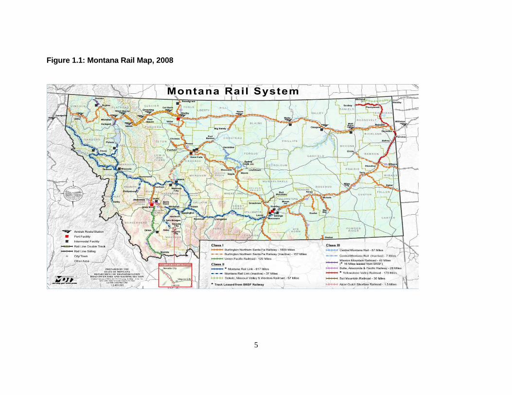
Table 1.1: Railroads Operating in Montana, 2008

Railroad Mileage Employees

Class IBurlington and Santa Fe Railway Company 2135 2,236Union Pacific 125 N/A

Class IIRegional Montana Rail Link 812 942

Dakota Missouri Valley and Western Railroad, Inc. 57 4

Local RailroadsCentral Montana Rail, Inc. 87 6

Montana Western Railway Co 59 16Rarus Railway Company 69 13

Source: Montana Department of Transportation

4

Intramodal competition is also limited in Montana. BNSF operates on 2,135

miles of track, while the only other Class I railroad in the state, UP, operates 125

miles of track. Regional operators include Montana Rail Link (MRL) and Dakota,

Missouri Valley and Western Railroad, Inc. (DMVWR). The regional classification

for DMVWR is misleading as the railroad only operates 57 miles of track in

Montana. While MRL operates a large amount of track (812 miles), it serves as a

bridge carrier for BNSF and consequently does not provide intramodal

competition. MRL operates and maintains the track, however BNSF still owns the

mainline. MRL must obtain permission from BNSF to perform interchange with

any other railroad and origins on the MRL line are treated as BNSF origins.

Furthermore, BNSF has agreed to provide a given level of bridge traffic on the line,

tying much of MRL traffic and financial health to that of BNSF. DMVWR is

affiliated with the Canadian Pacific Railroad (CP) and ties into CP lines in central

North Dakota. Other short lines include Central Montana Rail, Inc. (87 miles),

Montana Western Rail Co. (59 miles), and Rarus Railway Company (69 miles).

However each links to one or the other Class I railroads, thus not providing

competition. Figure 1 reflects the railroads operating in Montana in 2008.

Until recent years, hard red spring wheat has been the primary type of

wheat grown in Montana. As reflected in Table 1.2, 2007 spring wheat production

was just over 55.2 million bushels, while 2005 and 2006 production was 81.6 and

63.8 million bushels, respectively (NASS). The 2006 and 2007 production is

indicative of the impact of multiple years of drought in the region, causing the low

total wheat production since 2003. This has forced many customary spring wheat

5

Figure 1.1: Montana Rail Map, 2008

6

production areas to rotate to more drought sustainable winter wheat. Hard red

spring wheat production is primarily in the north central and northeast areas of the

state. These two areas accounted for over 42 million bushels of the 55 million

produced in 2007 (NASS). This area, while covering over 2.5 million acres in

cropped acres alone, is serviced almost exclusively by BNSF. Hard red spring

wheat is not produced in abundant quantities in barge competitive regions of the

country, suggesting that rail rates in Montana are unlikely to be constrained by

competing traffic in other regions that moves at lower rail rates. In other words,

geographic competition is unlikely to be significant for Montana wheat.

Table 1.2: Montana Wheat Production 2003 – 2007 (Thousands of Bushels)

Year Winter Wheat Durum Wheat Other Spring Wheat Total Wheat

2003 67,340 14,490 60,500 142,330

2004 66,830 17,985 88,350 173,165

2005 94,500 16,380 81,600 192,480

2006 82,560 6,715 63,800 153,075

2007 83,220 11,400 55,200 149,820

Total 394,450 66,970 349,450 810,870

Average 2003-2007 78,890 13,394 69,890 162,174Source: U.S. Department of Agriculture, National Agricultural Statistics ServiceRetrieved June 10, 2008 from http://www.nass.usda.gov/QuickStats

While there have been many studies of railroad pricing of agricultural

commodities, few of these have focused on Montana, where the competitive

restraints on rail grain prices appear to be minimal. The overall objective of this

thesis is to investigate railroad pricing behavior in the shipment of Montana wheat.

Specific objectives include the following:

7

1. Develop a model to measure the impacts of railroad costs and competition on

rail rates for Montana wheat.

2. Identify and measure the principal cost determinants of rail prices such as

distance, shipment volume, and weight per car.

3. Measure intramodal competition by comparing rail rates in a captive market

(Montana) to one with more intramodal competition (Kansas).

1.1 Thesis Statement Montana has limited intramodal competition for grain shipments across the

state and has been called a captive shipper due to the lack of rail competition. By

comparing a location with intramodal competition, would the presence of that

competition provide reduced shipping rates for wheat transportation in Montana?

1.2 Organization

The document is composed of six chapters and one appendix. Chapter 1 is

an introduction to the thesis topic and the organization of the paper. Chapter 2 is a

literature review, a summary of selected pertinent publications and their potential

application to the thesis. Chapter 3 is a discussion of the theoretical basis of the

research. Chapter 4 is a discussion of the research methods and the proposed

model to address the thesis problem. Chapter 5 is a discussion of the data

methods and the quantitative analysis of the topic. Chapter 6 is a discussion of the

findings of the research and its potential application. The attached appendix

includes additional reference information that may contribute to understanding of

the thesis.

8

CHAPTER 2: LITERATURE REVIEW

The depth of literature addressing the issue of competition in the railroad

transportation industry is significant, providing various degrees of analysis as to

the impact of competition within the industry. Much of the analysis investigates the

impact of deregulation after the Staggers Rail Act of 1980. A significant amount of

the literature is regional in scope and occurred in the decade post-Staggers.

Change continues within the railroad industry as both technology and infrastructure

advancements have occurred. These factors provide inherent limitations to the

findings of prior studies and will continue to do so with any such study as the

regional nature of the railroad transportation networks vary. What follows is not a

complete survey of the prior research conducted related to railroad competition;

however, the works cited provide a foundation and background for the

development of a railroad pricing model. Emphasis of this review is on the factors

that affect railroad competition on rail grain transportation prices.

The research article often cited in the works below is a piece entitled,

“Impact of the Staggers Rail Act on Agriculture: A Kansas Case Study”, Babcock,

Sorenson, Chow and Klindworth (1985). One objective of the study was to

describe and quantify rail initiatives in the Kansas wheat transportation market

following the implementation of the Staggers Act. They found in the four year

period of 1981 through 1984 substantial railroad reduction had occurred in the

level and arrangement of railroad rates. A pattern of rate changes suggested

competition among railroads and between individual railroads and truck-barge

9

combinations. They found that tariff rates to the Gulf of Mexico, in the post-

Staggers time frame had been reduced by 34%, compared to a 64% increase in

the four years preceding Staggers.

MacDonald (1989) examined Waybill samples as means of quantifying the

impact of deregulation on export grain rail shipping rates for wheat, corn and

soybeans. Using regression analysis, he found that interrail competition was

strongest for corn, and when rail service goes from monopoly to a duopoly, it leads

to a rate decline of 18%. Moving further to a triopoly, rates declined at a smaller

rate of 11%. He also found that access to water movement impacted rates as rail

rates increased as barge competition became less likely. This was most

noticeable on the rates associated with the transportation of wheat as wheat

origins are typically significantly greater distances from water than that of either

corn or soybeans. MacDonald found that shippers who were 400 miles from barge

access paid rates 40% more than those 100 miles away. He concluded that

concentration measures in all crop reporting areas indicated tight oligopolies and

the addition of a competitor makes a difference. Competition from barges has a

strong impact.

Chow (1986) examined rail grain rate changes for the Central Plains in the

post-Staggers period 1981-1986. He assessed the magnitude of rail rate

reductions for domestic and export markets as well as examined the change in

patterns of rates among rail firms within different regions of the Central Plains. His

analysis indicated an overall reduction in rates for wheat in the five year period

after Staggers of 34.5%, with the rate reductions occurring most significantly in the

10

export markets. He found that railroads adopted different strategies for rate-

adjustments with some being very consistent in their rate changes over their entire

systems, while others had greater rate reductions for some routes and less with

others. While rail contracts between carriers and shippers were not available for

the analysis, Chow asserted that the contract rates would be significantly lower

than the published rates. This would show a greater impact in the rate reductions

than the data used for the analysis indicated.

Adam and Anderson (1985) examined the effect of the Staggers Act on the

level of country elevator bid prices and if there was indeed an increase in bid

prices since Staggers passage. Using econometric models with corn and soybean

elevator bid prices in Nebraska, they found that both corn and soybean bid prices

were increased. However the impact on soybeans was higher at a level up to 14

cents per bushel. The impact on corn appeared to be offset by competing elevator

bids. However, the study also identified the buildup of capacity for the transport of

corn and the decline in the export market at the time, both exigent circumstances

such that the rail rate reduction was not seen in the increase of bid prices for corn.

The capacity build up during the time frame reflected the growth of unit train

activity. In 1977, there were only eight elevators in Nebraska with unit train

handling capabilities. By 1982 the growth in unit train handling facilities combined

with the decline in export markets provided over 200% of the capacity necessary

to move corn to the West Coast ports.

Kwon, Babcock, and Sorenson (1994) studied the impacts of Staggers in

the latter half of the 1980s as most prior studies investigated the impact

11

immediately post-Staggers. They investigated whether railroads have the ability to

practice differential pricing in a highly competitive and unregulated market as well

as sought to measure the determinants of rail differential pricing specific to the

transportation of Kansas wheat. Through the development of two econometric

models, one for intra Kansas shipments and one for export movements, to account

for the average car size differences (10 cars for intra Kansas and 20 for export);

they found that differential pricing was practiced by railroads in both cases. They

also found substantial differences in determining the factors affecting rate-to-

variable cost ratios (R/VC) for intra Kansas wheat movements versus that of export

Kansas wheat movements.

They observed that R/VC ratios increased steadily through the period of

1986 to 1989, however, they hypothesized it could have been the result of export

demand diminishing over the time frame. They also found that the disclosure of

previously confidential contracts reduced the incentive to negotiate contracts and

subsequently the published tariff rate was used by railroads and shippers. They

found that even though R/VC increased over the time frame, it may not have had a

negative consequence as a railroad received a 125.8 R/VC (at that time) and was

more likely to be able to provide adequate service and replace capital, versus that

of a railroad unable to cover its variable cost. Finally, they indicated geographic

competition is likely to constrain increases in R/VC rates for railroads within

Kansas for wheat as at some point increased R/VC railroad ratios will induce

diversion of Kansas wheat from Texas Gulf ports to other markets. This is also

likely the case for non-Kansas origins.

12

Fuller et al (1987) conducted a study to measure the impact of deregulation

on export-grain rates using a procedure that attempted to correct for shortcomings

of earlier research studies. The specified procedure controls for impact of events

which may be coincident with deregulation and, in addition, circumvents the

problem associated with inaccessible rate information included in the confidential

contracts. The procedure is applied to major export –grain transportation corridors

linking the central and south Plains and Corn Belt Regions with their respective

port areas.

The Fuller et al. study identified five regions that included the states of

Kansas, Iowa and Indiana as well as the Texas Panhandle and a portion of Illinois.

Kansas and The Texas Panhandle represented surplus producers of hard red

winter wheat, representing half of the U.S.’s annual wheat production and about

63% of wheat exports. Those regions rely heavily on rail for export transportation,

with 90% of western Kansas wheat transported on rail and 75% of northeast

Kansas and the Texas Panhandle wheat shipped by rail.

The effects of deregulation on export-grain railroad price structures were

identified with the analysis focusing on the price spread between port and

associated hinterland region. In general the adopted procedure involves the

estimation of regression equations which include hinterland’s farm-to-port price

spread (m) as the dependent variable and independent variables which control

shifts in demand and supply schedules; region and two dummies; a time trend ;

and a dummy and an interaction term to isolate changes in rates that may have

resulted from the 1980 Staggers deregulation.

13

Fuller et al. found deregulation to have had a significant effect on rail

transportation corridors linking the Plains states of Kansas and Texas with Gulf

ports and a relatively modest impact on the corridor linking Indiana with East Cost

ports. Kansas and Texas corridors had estimated real rate declines of $.37 and

$.31 per bushel during the 1981-1985 period. In the Indiana corridor, deregulation

is estimated to have decreased rates by $.08 per bushel. Additional analysis

indicated that the effect of deregulation in state subregions may have differed from

the estimated state wide effect.

The Iowa and Illinois regression models show deregulation to have had little

sustained statistically significant effect on rates in the regions linked with the Gulf

Ports. In contrast to the findings in the Plains, barge rates have an extremely

important effect on corridor price spreads. In the Illinois and Iowa models a dollar

decline in rates served to reduce the price spread by $.51 and $.73 per bushel

while the impact for Indiana was $.38 per bushel. To the analyst it seemed that

much of the decline in Corn Belt price spreads during the post-Staggers era can

be attributed to declining barge rates, not to a reduction in rail rates.

Koo, Tolliver and Bitzan (1993) investigated railroad pricing behavior in

North Dakota, a seemingly captive railroad shipping market focusing on the rail

transportation characteristics of the Upper Great Plains region. They argued that

the region had unique railroad transportation characteristics when compared to

other regions of the United States. These characteristics included limited

intermodal competition due to great distances to barge loading facilities and large

distances to major markets of consumption, processing and export. They

14

developed an econometric model applying data related to car weight, distance,

intramodal competition, intermodal competition and variables associated with three

respective crops, and the season of the year. Their research found that distance,

volume and weight per car all have significant negative effects on rates; intramodal

and intermodal competition had significant effects on rail rates suggesting that the

two Class I railroads in the state at the time were competing with each other and

with barge and truck movements from North Dakota.

Thompson, Hauser and Coughlin (1990) also evaluated the competitive

pressures on railroad rate-to-variable (R/VC) ratios for export shipments of corn

and wheat both pre- and post-Staggers. Through the development of four

regression models, two for corn and two for wheat, they found that the corn results

were less significant than those for wheat as shipment size for wheat likely reflects

the impact of expanded multi-car services post-Staggers. They found that there

was a lack of identifiable differences in pre- and post- deregulation pricing which

may be attributable to the close correlation between changes in certain operating

factors such as shipment size and destination opportunity. Their study concluded

that their results did not indicate a clear effect of the Staggers Rail act on rail rate

competitiveness.

These works and several others provide a collective review of the impact of

the Staggers Rail Act on competition and rail rates as well as some regional

considerations when one is examining the factors associated with rail rate

competition. Limitations were often identified and those factors should be

considered as one conducts further study of the topic. Furthermore, as addressed

15

in the introduction of this review, other factors associated with the rail

transportation industry have occurred in the time frame since several of these

works were completed, especially in Montana.

16

CHAPTER 3: THEORY

Examination of the markets that railroads operate in provides a basis for the

pricing that exists in the grain transportation sector. The theory to be examined

include those areas related to firms that operate in a particular market structure,

more specifically a railroad that operates with competition, as a monopoly, and

finally; as an oligopoly. The need for railroad reform will briefly be addressed

followed by a brief description of each market type and its application to railroad

transportation industry. The chapter concludes with an intermodal transportation

system theory review.

3.1 Railroad Reform Rationale

This paper has previously discussed many aspects of the Staggers

Railroad Act of 1980, typically in terms of impacts after the implementation of the

legislation. The implementation of Staggers was seen as a necessary tool to

promote the reform necessary for the financial well being of the railroad industry.

Through the 1950s widespread financial problems arose and in the late 1960s and

early 1970s several railroads in the eastern U.S. filed for bankruptcy. Government

intervention in the northeastern railroad network formed the Conrail system after

financial collapse of the one of the major eastern carriers. Through the late 1970s

bankruptcy was also experienced with the three Midwestern railroads, one of

which, the Milwaukee Road, had trackage through Montana.

These railroad failures brought on the political necessity to implement

reform with the first major reform act, the Rail Revitalization and Regulatory

17

Reform (4R) of 1976. The act allowed improved pricing flexibility while easing

restrictions for abandonments. The Interstate Commerce Commission (ICC)

rather restrictively interpreted the act and important changes did not occur until the

ICC composition changed in 1979. This led to the ICC approving four major

mergers, accelerated abandonments and the introduction of confidential contract

rates. These actions preceded the passage of the Staggers Act in 1980 and in

some respects; Staggers validated the reform that ICC had already implemented.

These measures were necessary to restore the financial viability of railroads and

have contributed to the sustainability of the railroad transportation network within

the U.S. today.

3.2 Perfect Competition Perfect competition in a market will reflect pricing according to the market

supply and demand curves. Increases in prices are represented on a supply curve

to slope upward to the right resulting in increased industry output. The market

demand curve slopes downward and toward the right, as prices increase, demand

for the product is reduced. Essentially, the key aspect in a perfectly competitive

market is that maximum profit exists at the output where marginal revenue (price)

is equal to the output price. (Mansfield 2002). Further, the barriers to entry are

very low, requiring only a small investment to enter the industry. There are a very

large number of buyers and sellers, and the product is homogeneous. In the

railroad industry, perfect competition is likely non-existent as there are a limited

number of firms that actually compete. The resources necessary to enter the

18

market discourage entry by others as a significant capital investment is required to

build and operate a railroad.

3.3 Monopoly In a monopoly, the industry consists of one firm; a single seller of the

product or service. A monopolist will have considerable control over pricing as

there is no additional competitor in the industry. A monopolist in an unregulated

market, if it maximizes profit, will price its product and produce the output at a point

where marginal revenue is equal to marginal cost and marginal revenue is derived

from the demand curve. A monopolist, when free of direct competitor imposed

restraints, can set higher prices, and generate higher profits than it would if it were

exposed to the competition of a rival firm. Entry to the market is essentially

blocked.

Railroads reflect characteristics of a monopoly in a regional perspective

throughout the U.S. There are also locations where there is more then one

railroad firm that may provide intermodal competition. However, as discussed

previously, the industry does experience intermodal competition from other firms

within the transportation industry (barge and truck). Furthermore, railroads are

subject to government regulation limiting the ability of the industry to act as a true

monopolist in those areas that lack firm competition.

3.4 Oligopoly An oligopoly is an intermediate situation between that of perfect competition

and a monopoly where there only a few firms competing in a market. An oligopoly

is likely going to have less control over pricing than that of a monopoly, but more

19

than that of a perfectly competitive firm. Barriers to entry are high in oligopoly and

they tend to rely heavily on nonprice competition.

Oligopoly competition most accurately reflects railroads as grain shippers

can utilize other modes (barge and truck) in some cases to transport grain to

domestic markets.

3.5 Intermodal Transportation System Theory Grain shippers utilize three modes of transport to ship grain to markets: (1)

rail, (2) truck, and (3) water. The least cost mode for a given grain shipment is a

function of distance from origin to destination. In Figure 1, hypothetical modal cost

curves are constructed for the rail, truck, and water modes between origin i and

destination j. The hypothetical cost curve for trucking (T) indicates that trucks have

a cost advantage for short hauls because they have insignificant fixed and terminal

costs relative to other modes. The cost curve for water shipment (W) shows that

water movements have the lowest unit costs with respect to distance but

significantly higher fixed or terminal costs than other modes. Thus water has the

highest trip costs for short distance movements and the lowest costs for long haul

shipments. The railroad cost structure (R) lies between the short haul cost

advantage of trucks and the long haul advantage of water shipment.

While the cost curves in Figure 1 are linear to simplify the modal relationships,

costs increase at a decreasing rate with distance due to economies of long hauls.

Carriers realize economies of long haul primarily because fixed terminal costs are

spread over a great number of miles. If the freight rate is determined solely by

costs, the transport market will be divided among modes, according to distance,

20

holding all other rate factors constant. Thus in Figure 1, motor carriers will have a

cost advantage for distance OC, railroads will have the cost advantage for distance

CD, and water will have the advantage for distances greater than OD.

Figure 3.1: Hypothetical Trip Cost Curves for Rail (RR’), Truck (TT’), and Water (WW’), Modes of Transportation for a given Origin/Destination

In addition to cost factors such as distance, competitive factors have an

impact on rail rates. Intermodal and intramodal competition constrains rail market

power, and in markets where such competition exists, railroads will charge lower

rates than in non-competitive markets.

3.6 Theoretical Model The theoretical model is a variant of the model published in Koo et al

(1993). Equilibrium prices of rail transport of agricultural products are determined

by demand for and supply of rail service. Demand for a railroad's service (qd) is a

function of the price of the railroad's service (p1), the price of other railroads'

0 C D

AB

W

R

T

T´

R´ W´

Distance

Tri

p C

ost

21

transport service (p2, p3... ), the prices of other modes of transport (a1, a2, ... ),

and other factors affecting demand for rail transport (S). Thus the demand

function is equation (1).

(1) qd = fd(p1, p2, p3…, a1, a2, S)

The supply of a railroad's service is a function of the price of the

railroad’s service (p1), cost factors such as distance (d) and shipment volume

(v), and other variables that affect the cost of rail service (C). Thus the supply

function is equation (2).

(2) qs = fs(p1, d, v, C )

In equilibrium, qd = qs, so equations (1) and (2) can be combined to form

the equilibrium condition. Thus the equilibrium price equation for railroad (1) is as

follows:

(3) p1 = f1(p2, p3, …, a1, a2, d, v, S, C )

All the variables in equation (3) are as defined above.

If the prices of other railroads (p2, p3) are defined as intramodal competition

(iac) and the prices of other modes (a1, a2...) are defined as intermodal

competition (ioc), then equation (3) can be rewritten as follows:

(4) p1 = f(iac, ioc, v, S, C)

The following chapter applies the theoretical model to the empirical model

to achieve the objectives of the study.

22

CHAPTER 4: EMPIRICAL MODEL

The theoretical model from the previous chapter is modified to achieve the

objectives of the study. As discussed in Chapter 3, intermodal competition is likely

to be minimal for rail shipments of Montana wheat. The great majority of the

shipments are long distance movements to Portland, making truck competition

ineffective. The average distance to a water port is 522 miles rendering barge

competition to be non-existent. The BNSF dominates the rail industry in Montana

so intramodal competition is non-existent as well. The empirical model is specified

as follows where all continuous variables are specified as natural logarithms so the

coefficients are elasticity’s.

(1) CWT = β0 + β1CARWT + β2DIST + β3GVW + β4BARGE + β5DUMMY + εi

CWT - Rail rate in dollars per cwt-mile for the shipment

CARWT - Weight (lbs) of each loaded covered hopper rail car in a shipment

DIST - Distance in rail miles between origins and export port

GVW - Total shipment weight in tons

BARGE - Distance of origin to barge loading facilities

DUMMY - Dummy variable to represent either a Montana or Kansas location,

Montana being assigned 1 and Kansas 0

ε - random error term

The dependent variable (CWT) is the rail rate per hundred weight (cwt)-mile

and can be obtained by dividing total revenue of the shipment by weight and

distance. Calculation is further demonstrated in Table 4.1. Variation in total

23

revenues of the shipment is obtained by varying the number of cars in the train,

and variation in distance is obtained by varying the origin of the shipment. The total

shipment weight (GVW) is obtained by varying the number of carloads in the train

and multiplying by the weight per car (CARWT). The distance variable (DIST) is

the distance from various origins in Montana to Portland, Oregon and from various

origins in Kansas to Houston, Texas. The distance of the origin to barge loading

facilities (BARGE) is the distance from Montana origins to Lewiston, Idaho for the

Montana equation, and the distance from Kansas origins to Kansas City, Missouri

in the Kansas equation. Variation in weight per car (CARWT) is introduced by

assuming various car sizes, i.e., 268,000 pound cars vs. 286,000 pound cars.

Figure 4.1: Method for Calculation for BNSF Rates Per Cwt-Mile

(1) Total Revenue of Shipment = Number of cars in the shipment x rate per car.

(2) Weight of the Shipment = Number of cars in the shipment x weight per car/100.

(3) Divide (1) by (2) to get Revenue per cwt. (4) Divide (3) by distance of shipment to get Revenue per cwt-mile. (5) Multiply (4) by 1000 to get into integer form.

The theoretically expected sign of the natural log of the distance variable is

negative. A large share of railroad costs are fixed with respect to distance, such as

loading and clerical costs, insurance, taxes, interest, and managerial overhead. As

these costs are spread over more miles, the costs per mile decrease at a

decreasing rate, so the change in the rail rate per cwt-mile falls as distance

increases.

24

The GVW variable reflects (a) the number of cars in the shipment, and (b)

the weight per car. Since the empirical model includes the commodity weight per

car (CARWT), the volume variable reflects the impact on rail rates of increased

cars in the shipment. Because a large share of rail costs are fixed with respect to

weight, railroads also realize economies of weight. Thus the change in rail rates

per cwt-mile are expected to decrease at a decreasing rate as volume increases.

Intermodal competition is measured by highway miles to water ports. Longer

distances to water access points reduce the feasibility of truck-barge competition

for rail wheat shipments. Thus, the theoretically expected sign of BARGE is

positive since the greater the distance to water ports the greater the pricing power

of railroads.

Weight per car (CARWT) is expected to have a negative relationship to the

change in rail rates per cwt-mile. Because operating costs such as switching costs

per car, labor costs, clerical costs, and various other costs are fixed per car, these

costs per car decrease as car weight increases. Thus the change in rail rates per

cwt-mile fall as car weight rises.

The empirical model is estimated for Montana and Kansas. For Montana,

the shipments in the empirical model are from Montana wheat origins to Portland,

Oregon for export. For Kansas, the modeled wheat shipments are from Kansas

origins to the export ports at Houston. Like Montana, intermodal competition is

limited in the Kansas wheat transport market. The distance to Houston makes

truck competition non-existent, and historically only negligible amounts of Kansas

wheat have been shipped on the Missouri and Arkansas Rivers. However, unlike

25

Montana, Kansas is served by both the BNSF and UP. The lines of the two

railroads are in close physical proximity in many cases, and they have roughly the

same number of Kansas track miles (1,260 miles for BNSF and 1,505 miles for

UP). Then intramodal competition is introduced by pooling the data of the two

states and inserting a dummy variable in the equation for all Montana

observations.

26

CHAPTER 5: DATA AND EMPIRICAL RESULTS 5.1 Data The model is estimated, using rates published on the BNSF website

(www.bnsf.com.) for wheat movements in Montana to Portland and Kansas to

Houston. This is believed to be the best data available as it represents accurate

shipping charges published by BNSF. The published rates were taken from the

website on November 4, 2008 for each respective car type and train size. The

BNSF website was further used to gather the rail shipping miles from each origin to

the port destination.

Table 5.1: Montana and Kansas Truck Miles from Origins

Truck Mileage to nearest barge facility - Montana origins to Lewiston, ID

Glendive 786Harlem 452Collins 410 AveragePompeys 597 511Shelby 449Carter 413.5Rudyard 511Grove 467

Truck Mileage to nearest barge facility - Kansas origins to Kansas City, MO

Wichita 199Wellington 226Salina 175 AverageHutchinson 217 239Garden City 387.5Dodge City 335Concordia 223Abilene 151

27

The model uses eight locations in Kansas and Montana identified in Table

5.1. The table also identifies the distance in miles to the nearest barge location.

Other data used for the model included distance in rail miles from points of origin

to export in Montana and Kansas respectively. The wheat export destination for all

Montana origins was Portland, Oregon; while the wheat export location for all

Kansas locations was Houston, Texas.

Table 5.2: Mean and Standard Deviation of Variables

Variables CARWT DIST GVW BARGE CWT

Combined Mean 277000 886.567 11697.923 427.212 1.325Combined Standard Deviation 9021.713 152.516 5679.549 165.155 0.228

Montana Mean 277000 946.875 11141.556 510.750 1.252Montana Standard Deviation 9031.414 137.490 5655.667 118.677 0.178

Kansas Mean 277000 750.875 12949.750 239.250 1.487Kansas Standard Deviation 9071.147 80.649 5575.328 76.233 0.244

Table 5.2 is the mean and the standard deviation of the data series for the

variables. The mean and standard deviation is reflected for the combined data

series and Montana and Kansas individually. Table 5. reflects the Montana and

Kansas locations and the respective rail mileage for each.

28

Table 5.3: Montana and Kansas Rail Miles from Origins

OriginGlendiveHarlemCollinsPompeysShelbyCarterRudyardGrove

Rail mileage Montana Origins to Portland, Oregon

Rail Mileage1245925839

1054785909849969

OriginWichitaWellingtonSalinaHutchinsonGarden CityDodge CityConcordiaAbilene

Rail mileage Kansas Origins to Houston, Texas

Rail Mileage646631775

752

702872822807

5.2 Empirical Results Table 5.3 reflects the results of the regression estimated with ordinary

least squares. Model outcome has an adjusted R-squared of 0.74 and the

standard error of regression is 0.11 with the standard dependent variable at 0.22.

Probability factor for each variable is close to zero with CARWT having the highest

level of 0.0047. The signs and magnitudes of the statistically significant

parameters appear reasonable given the outlined theoretical framework.

29

Table 5.4: Railroad Rate Regression Equation

Method: Least SquaresSample: 208Included observations: 208

Variable Coefficient Std. Error t-Statistic Prob. C 1.860065 0.253147 7.347764 0CARWT 2.52E-06 8.82E-07 2.859597 0.0047DIST -0.001199 0.000124 -9.644381 0GVW -2.28E-05 1.42E-06 -16.10731 0BARGE 0.000519 0.000142 3.651677 0.0003DUMMY -0.182486 0.027907 -6.539061 0

R-squared 0.754499 Mean dependent var 1.324604Adjusted R-squared 0.748422 S.D. dependent var 0.227749S.E. of regression 0.114233 Akaike info criterion -1.472723Sum squared resid 2.635955 Schwarz criterion -1.376448Log likelihood 159.1632 F-statistic 124.1611Durbin-Watson stat 1.11315 Prob(F-statistic) 0

All the explanatory variables were statistically significant at the .01 level

except for CARWT. Independent variables DIST and GVW had the theoretically

expected negative sign, while BARGE had the expected positive sign. The

expected sign of CARWT is negative, so the positive sign was not expected.

However, given the small size of the coefficient, CARWT has minimal impact on

the dependent variable.

The most unexpected result was the statistically significant negative sign for

the dummy variable, indicating that wheat rail rates are lower in Montana than

Kansas. This finding does not agree with previous research with found that rail

wheat rates are higher in North Dakota and Montana compared to the other wheat

producing areas. The reasons for the observed higher wheat rail rates in Montana

are a topic for further research.

30

CHAPTER 6: CONCLUSION

The objectives of this thesis were to develop a model to measure railroad

costs and competition; determine the principal cost determinants and measure

intramodal competition by comparing the rates in a captive market (Montana) to

one with more intramodal competition (Kansas).

The empirical model reflects key cost components and competition impacts

on the rates associated with rail shipments of wheat out of Montana and Kansas.

The empirical model regression outcomes reflect a reasonable goodness of fit for

the variables established as determinants of cost. The model indicates rates of a

captive market like Montana may not be higher then those with more intramodal

competition such as Kansas.

Because this finding doesn’t agree with previous research, other factors

may contribute to the price determinants of rail competition and further study such

as a revenue to variable cost assessment may find similar findings of prior

research.

31

REFERENCES Adam, Brian G. and Dale G Anderson. “Implications of the Staggers Rail Act of

1980 for the Level and Variability fo County Elevator Price Bids.” Proceedings of the Transportation Research Forum 26(1), (1985): 357-363.

Babcock, Michael W., L. Orlo Sorenson, Ming H. Chow, and Keith Klindworth.

“Impact of Staggers Rail Act on Agriculture: A Kansas Case Study.” Proceedings of the Transportation Research Forum 26(1), (1985): 364 -372.

Chow, Ming H. “Interrail Competition in Rail Grain Rates on the Central Plains.”

Proceedings of the Transportation Research Forum 27(1), (1986): 164 -171. Fuller, Stephen, David Bessler, James MacDonald, Michael Wohlgenant. “Effects

of Deregulation on Export-Grain Rail Rates in the Plains and Corn Belt.” Proceedings of the Transportation Research Forum 28(1), (1987): 160 -167.

Koo, Won W., Denver D. Tolliver and John D. Bitzan. “Railroad Pricing in Captive

Markets: An Empirical Study of North Dakota.” Logistics and Transportation Review 29(2), (1993)): 123 -137.

Kwon, Y.W., Michael W. Babcock, Orlo I. Sorenson. “Railroad Differential Pricing

in Unregulated Transportation Markets: A Kansas Case Study.” The Logistics and Transportation Review 30 (3), (1994): 223 -244.

MacDonald, James M. “Competition and Rail Rates for the Shipment of Corn,

Soybeans and Wheat.” Rand Journal of Economics 18(1), (1987): 151-163. MacDonald, James M. (1989). Effects of Railroad Deregulation on Grain

Transportation, U.S. Department of Agriculture, ERS Technical Bulletin No. 1759, Washington D. C.

Mansfield, E. “Managerial Economics: Theory, Applications, and Cases” 5th. Ed.

W.W. Norton and Company 2002. Thompson, S.R., R. J. Hauser and B.A. Coughlin. “The Competitiveness of Rail

Rates for Export-Bound Grain.” The Logistics and Transportation Review 26(1), (1990): 35-53.