analysis of propagation models for wimax at 3.5 ghz830403/fulltext01.pdf · okumura model, hata...

1

MEE 09:59

Analysis of Propagation Models for WiMAX at

3.5 GHz

By

Mohammad Shahajahan and A. Q. M. Abdulla Hes-Shafi

This thesis is presented as part of Degree of

Master of Science in Electrical Engineering

Blekinge Institute of Technology

September 2009

Department of Electrical Engineering


SE – 371 79 Karlskrona

Sweden

2

This thesis is submitted to the Department of Electrical Engineering at Blekinge Institute of

Technology in partial fulfilment for the degree of Master of Science in Electrical Engineering.

The thesis is equivalent to 20 weeks of full time studies.

Contact Information:

Author(s):

Mohammad Shahajahan

E-mail:[email protected]

A.Q.M. Abdulla Hes-Shafi E-mail: [email protected]

Supervisor:

Professor Hans-Jürgen Zepernick E-mail: [email protected]

School of Engineering


Phone: + 46457385718

Mobile: + 46708782680


Sweden

Examiner:

Professor Hans-Jürgen Zepernick E-mail: [email protected]

School of Engineering


Phone: + 46 457 385718

Mobile: + 46 708782680


Sweden

3

Dedicated to our parents

4

Abstract

Nowadays the Worldwide Interoperability of Microwave Access (WiMAX) technology becomes

popular and receives growing acceptance as a Broadband Wireless Access (BWA) system.

WiMAX has potential success in its line-of-sight (LOS) and non line-of-sight (NLOS) conditions

which operating below 11 GHz frequency. There are going to be a surge all over the world for the

deployment of WiMAX networks. Estimation of path loss is very important in initial deployment

of wireless network and cell planning. Numerous path loss (PL) models (e.g. Okumura Model,

Hata Model) are available to predict the propagation loss, but they are inclined to be limited to

the lower frequency bands (up to 2 GHz). In this thesis we compare and analyze five path loss

models (i.e. COST 231 Hata model, ECC-33 model, SUI model, Ericsson model and COST 231

Walfish-Ikegami model) in different receiver antenna heights in urban, suburban and rural

environments in NLOS condition. Our main concentration in this thesis is to find out a suitable

model for different environments to provide guidelines for cell planning of WiMAX at cellular

frequency of 3.5 GHz.

5

Acknowledgements

All admires to Almighty ALLAH, the most gracious and the most merciful, who bequeathed us

with wellbeing and abilities to complete this project successfully.

We wish to express our deep gratitude to our project supervisor Professor Hans-Jürgen Zepernick

for his continuous heart and soul support to complete the project in the best possible way. He is

always a source of inspiration and motivation for us. His encouragement and support never

faltered.

We are especially thanks to the Faculty and Staff of School of Engineering at the Blekinge

Institute of Technology (BTH), Karlskrona, Sweden, who have been supported us immensely

during this research.

We are also very thankful to our entire fellow colleague‟s who have helped us mentally as well as

academically, in every hour of necessitate.

Finally, we are wildly grateful to our parents for their everlasting moral support and

encouragements. It is to them we dedicated this project.

Mohammad Shahajahan & A.Q.M. Abdulla Hes-Shafi

Ronneby, September 2009.

6

TABLE OF CONTENTS

Contents Blekinge Institute of Technology .................................................................................................. 1

Abstract ............................................................................................................................................ 4

Acknowledgements ........................................................................................................................... 5

TABLE OF CONTENTS ................................................................................................................. 6

CHAPTER 1 ..................................................................................................................................... 8

Introduction ...................................................................................................................................... 8

1.1 Motivation .............................................................................................................................. 8

1.2 Background of Propagation Models ..................................................................................... 11

1.3 Research Goals ..................................................................................................................... 12

1.4 Thesis Outline ...................................................................................................................... 13

CHAPTER 2 ................................................................................................................................... 14

Review of the state of art ................................................................................................................ 14

2.1 IEEE 802.16 working group ................................................................................................. 14

2.1.1 IEEE 802.16a ................................................................................................................ 14

2.1.2 IEEE 802.16-2004 ......................................................................................................... 15

2.1.3 IEEE 802.16e-2005 ....................................................................................................... 15

2.2 Features of WiMAX ............................................................................................................. 16

2.3 Frequency band selection ..................................................................................................... 19

CHAPTER 3 ................................................................................................................................... 20

Principal of Propagation Models .................................................................................................... 20

3.1 Types of Propagation Models .............................................................................................. 20

3.2. Basic Propagation Mechanisms .......................................................................................... 22

3.3 Necessity of Propagation Models ......................................................................................... 23

CHAPTER 4 ................................................................................................................................... 25

Path Loss Models ........................................................................................................................... 25

4.1 Free Space Path Loss Model (FSPL) ................................................................................... 25

4.2 Okumura Model ................................................................................................................... 25

4.3 COST 231 Hata Model ......................................................................................................... 27

4.4 Stanford University Interim (SUI) Model ............................................................................ 28

4.5 Hata-Okumura extended model or ECC-33 Model .............................................................. 31

4.6 COST 231 Walfish-Ikegami (W-I) Model ........................................................................... 32

7

4.7 Ericsson Model ..................................................................................................................... 35

CHAPTER 5 ................................................................................................................................... 37

Simulation of Models ..................................................................................................................... 37

5.1 Path loss in urban area .......................................................................................................... 38

5.2 Path loss in suburban area .................................................................................................... 41

5.3 Path loss in rural area ........................................................................................................... 44

CHAPTER 6 ................................................................................................................................... 47

Analysis of simulation results in urban area .................................................................................. 47

Analysis of simulation results in suburban area ............................................................................. 48

Analysis of simulation results in rural area .................................................................................... 49

CHAPTER 7 ................................................................................................................................... 50

Conclusions .................................................................................................................................... 50

Future work .................................................................................................................................... 51

APPENDICES ................................................................................................................................ 52

Appendix-A: Simulation process flow chart for three different environments .......................... 52

Appendix-B: MATLAB Code for Urban environment in different antenna heights ................. 53

Appendix-C: MATLAB Code for Suburban environment in different antenna heights ............ 55

Appendix-D: MATLAB Code for rural environment in different antenna heights ................... 57

Appendix-E: Abbreviations and Acronyms ............................................................................... 59

References ...................................................................................................................................... 61

8

CHAPTER 1

Introduction

Nowadays people are enjoying wireless internet access for telephony, radio and television

services when they are in fixed, mobile or nomadic conditions. The rapid growth of wireless

internet causes a demand for high-speed access to the World Wide Web. To serve the demand for

access to the internet „any where any time‟ and ensure quality of service, the IEEE 802.16

working group brought out a new broadband wireless access technology called “WiMAX”

meaning Worldwide Interoperability for Microwave Access.

Broadband Wireless Access (BWA) systems have potential operation benefits in Line-of-sight

(LOS) and Non-line-of-sight (NLOS) conditions, operating below 11 GHz frequency. During the

initial phase of network planning, propagation models are extensively used for conducting

feasibility studies. There are numerous propagation models available to predict the path loss (e.g.

Okumura Model, Hata Model), but they are inclined to be limited to the lower frequency bands

(up to 2 GHz). In this thesis we compare and analyze five path loss models (e.g. COST 231 Hata

model, ECC-33 model, SUI model, Ericsson model and COST 231 Walfish-Ikegami (W-I)

model) which have been proposed for frequency at 3.5 GHz in urban and suburban and rural

environments in different receiver antenna heights.

1.1 Motivation

Worldwide Interoperability for Microwave Access (WiMAX) is the latest broadband wireless

technology for terrestrial broadcast services in Metropolitan Area Networks (MANs). It was

introduced by the IEEE 802.16 working group to facilitate broadband services on areas where

cable infrastructure is inadequate. It is easy to install and cheap. It provides triple play

applications i.e. voice, data and video for fixed, mobile and nomadic applications. The key

features of WiMAX including higher bandwidth, wider range and area coverage, its robust

flexibility on application and Quality of Services (QoS) attract the investors for the business

scenarios. Now the millions of dollar are going to be invested all over the world for deploying

9

this technology. The following Table 1.1 on commercial report [5] shows the expected

development of WiMAX networks over the last three years all over the world by region.

Table 1.1: Growth of Global WiMAX Deployment by Region Oct 2008 [5]

WiMAX

Networks Area

September-2006 September-2007 September-2008

North America 0 9 14

Latin America 4 11 22

Western Europe 5 17 21

Eastern Europe 9 14 18

Africa 2 8 21

Middle East 0 1 4

Asia and Pacific 6 13 26

This BWA technology is based on Orthogonal Frequency Division Multiplex (OFDM)

technology and considers the radio frequency range up to 2-11 GHz and 10-66 GHz. Propagation

condition under NLOS is possible by using OFDM, which opens the possibility of reliable and

successful communication for wireless broadband. An important feature is an adaptive

modulation technique, which depends on Signal to Noise Ratio (SNR). It ensures transmission

during difficult condition in propagation or finding weak signal in the receiver-end by choosing a

more vigorous modulation technique.

In an ideal condition, WiMAX recommends up to 75 Mbps of bit rate and range within 50 km in

the line of sight between transmitter and receiver [2]. But in the real field, measurements show

far differences from ideal condition i.e. bit rate up to 7 Mbps and coverage area between 5 and 8

km. To reach the optimal goal, researchers identified the following becomes that impair the

transmission from transmitter to receiver.

Path loss

Co-channel and adjacent-channel interference

Fading

Doppler spread

10

Multipath delay spread

Path loss (PL): Path loss arises when an electromagnetic wave propagates through space from

transmitter to receiver. The power of signal is reduced due to path distance, reflection,

diffraction, scattering, free-space loss and absorption by the objects of environment. It is also

influenced by the different environment (i.e. urban, suburban and rural). Variations of transmitter

and receiver antenna heights also produce losses. In our thesis we mainly focus on path loss

issue. In general it is expressed as:

PL= in dB.

Co-channel and adjacent-channel interference: Co-channel interference or crosstalk occurs

when same frequency is used by two different transmitters. Adjacent-channel interference (ACI)

arises when a signal gained redundant power in an adjacent channel. It is caused by many reasons

like improper tuning, incomplete or inadequate filtering or low frequency. In our thesis, we use

3.5 GHz frequency, which is licensed band. But it may be interfered by the other competing

Fixed Wireless Access (FWA) operators who are using the adjacent frequency in the same

territory or same frequency in the adjacent territory.

Fading: Fading is a random process; a signal may experience deviation of attenuation due to

multipath propagation or shadowing in any obstacles in certain broadcast media.

Doppler spread: A mobile user causes a shift in the transmitted signal path by its velocity. This

is known as Doppler shift. When signals travelled in different paths, thus may experience

different Doppler shifts with different phase changes. Contributing a single fading channel with

different Doppler shift is known as the Doppler spread.

11

Delay spread: A signal arrives at its destination through different paths and different angels.

There is a time difference between the first multipath received signal (usually line-of-sight signal)

and the last received signal, which is called delay spread.

1.2 Background of Propagation Models

By combining analytical and empirical methods the propagation models is derived. Propagation

models are used for calculation of electromagnetic field strength for the purpose of wireless

network planning during preliminary deployment. It describes the signal attenuation from

transmitter to receiver antenna as a function of distance, carrier frequency, antenna heights and

other significant parameters like terrain profile (e.g. urban, suburban and rural).

Models such as the Harald.T. Friis free space model are used to predict the signal power at the

receiver end when transmitter and receiver have line-of-sight condition. The classical Okumura

model is used in urban, suburban and rural areas for the frequency range 200 MHz to 1920 MHz

for initial coverage deployment. A developed version of Okumura model is Hata-Okumura model

known as Hata model which is also extensively used for the frequency range 150 MHz to 2000

MHz in a build up area.

Comparison of path loss models for 3.5 GHz has been investigated by many researchers in many

respects. In Cambridge, UK from September to December 2003 [1], the FWA network

researchers investigated some empirical propagation models in different terrains as function of

antenna height parameters. Another measurement was taken by considering LOS and NLOS

conditions at Osijek in Croatia during spring 2007 [2]. Coverage and throughput prediction were

considered to correspond to modulation techniques in Belgium [3].

Numerous models are used for estimating initial deployment. In the following Table 1.2, we

briefly described some models with frequency ranges for understanding the importance of studies

at the carrier frequency of 3.5 GHz.

12

Table 1.2: Well known propagation models [9].

Models Frequency

Range

Applicable Different terrain

support/comments

ITU Terrain Model Any LOS Support all terrains/based

on diffraction theory

Egli model Not specified LOS Not applicable in the

foliage area

Early ITU model Not specified LOS Support vegetation

obstacles/ suitable for

microwave link

Weissberger‟s model 230 MHz-95 GHz LOS Only applicable when

foliage obstruction in the

microwave link

Okumura model 200 MHz-1920 MHz LOS/NLOS Ideal in the city area

Hata model 150 MHz-1500 MGz LOS/NLOS Support all terrains/ limited

antenna height 10 m. in

small city

Lee model (Area to Area) 900 MHz LOS/NLOS Use more correction factors

to make it flexible in all

conditions

Lee model (Point to point) 900 MHz LOS Use more correction factors

to make it flexible in all

conditions

Longley –Rice model 20 MHz-20 GHz LOS/NLOS Suitable in VHF and UHF

use

1.3 Research Goals

Today the challenge is how to predict the path loss at the cellular frequency of 3.5 GHz. There

are several empirical propagation models which can precisely calculate up to 2 GHz. But beyond

2 GHz, there are few reliable models which can be referred for the WiMAX context. There are

few proposed models [1]-[4], which focus on frequency range at 3.5 GHz out of which we base

our analysis. In this paper, we compare and analyze path loss behaviour for some proposed

models at 3.5 GHz frequency band. Our research goal is to identify a suitable model in different

environments by applying suitable transmitter and receiver antenna heights. Thus, a network

engineer may consume his/her time by using our referred model for deploying the initial planning

13

in different terrains.

1.4 Thesis Outline

The thesis is organized in the following order: In Chapter 2, we discussed some basic features of

WiMAX technology. In Chapter 3, the principle of propagation mechanisms are described. In

Chapter 4, some path loss models are introduced. In Chapter 5, simulation output of all models is

presented. In Chapter 6, we compare and analyze all simulated data. In Chapter 7, the conclusions

of the thesis and future research are presented.

14

CHAPTER 2

Review of the state of art

To take the edge off the dream to access broadband internet „anywhere-anytime‟, the IEEE

formed a working group called IEEE 802 16 to make standards for wireless broadband in

Metropolitan Area Network (MAN). The working group introduced a series of standards for

fixed and mobile broadband internet access known by the name “WiMAX”. This name is given

by the WiMAX Forum (an industry alliance responsible for certifying WiMAX products based

on IEEE standards). In this chapter, we discussed on IEEE 802.16 family and some important

features of WiMAX.

2.1 IEEE 802.16 working group

After successful implementation of wireless broadband communication in small area coverage

(Wi-Fi), researchers move forward for the wireless metropolitan area network (WMAN). To find

the solution, in 1998, the IEEE 802.16 working group decided to focus their attention to gaze on

new technology. In December 2001, the 802.16 standard was approved to use 10 GHz to 66 GHz

for broadband wireless for point to multipoint transmission in LOS condition. It employs a single

career physical (PHY) layer standard with burst Time Division Multiplexing (TDM) on Medium

Access Control (MAC) layer [10].

2.1.1 IEEE 802.16a

In January 2003, another standard was introduced by the working group called, IEEE 802.16a,

for NLOS condition by changing some previous amendments in the frequency range of 2 GHz to

11GHz. It added Orthogonal Frequency Division Multiplexing (OFDM) on PHY layer and also

uses Orthogonal Frequency Division Multiple Access (OFDMA) on the MAC layer to mitigate

“last mile” fixed broadband access [10].

15

2.1.2 IEEE 802.16-2004

By replacing all previous versions, the working group introduced a new standard, IEEE 802.16-

2004, which is also called as IEEE 802.16d or Fixed WiMAX. The main improvement of this

version is for fixed applications.

2.1.3 IEEE 802.16e-2005

Another standard IEEE 802.16e-2005 approved and launched in December 2005, aims for

supporting the mobility concept. This new version is derived after some modifications of

previous standard. It introduced mobile WiMAX to provide the services of nomadic and mobile

users.

The details of WiMAX system profiles are presented here at a glance, i.e., operating frequencies,

multiplexing, and modulation techniques, channel bandwidth (see Table 2.1).

Table.2.1: Specifications of IEEE 802.16 at a glance [10]

Features 802.16a 802.16d-2004 802.16e-2005

Status Completed

December 2001

Completed

June 2004

Completed

December 2005

Application Fixed Loss Fixed LOS Fixed and Mobile NLOS

Frequency Band 10 GHz-66 GHz 2 GHz – 11 GHz 2 GHz- 11 GHz for Fixed.

2 GHz- 6 GHz for Mobile

Modulation QPSK,16-QAM,

64-QAM

QPSK,16-QAM,

64-QAM

QPSK,16-QAM,

64-QAM

Gross Data Rate 32 Mbps - 134.4 Mbps 1Mbps-75Mbps 1 Mbps-75 Mbps

Multiplexing Burst

TDM/TDMA

Burst

TDM/TDMA/ OFDMA

Burst

TDM/TDMA/OFDMA

Mac Architecture Point-to-Multipoint,

Mesh

Point-to-Multipoint,

Mesh

Point-to-Multipoint,

Mesh

Transmission Scheme Single Carrier only Single Carrier only,

256 OFDM or 2048 OFDM

Single Carrier only, 256

OFDM or scalable OFDM

with 128, 512, 1024, 2048

sub-carriers

Duplexing TDD and FDD TDD and FDD TDD and FDD

16

2.2 Features of WiMAX

Nowadays, WiMAX is the solution of “last mile” wireless broadband. It provided an enhanced

set of features with flexibility in terms of potential services. Some of them are highlighting here:

Interoperability:

Interoperable is the important objective of WiMAX. It consists of international, vendor-neutral

standards that can ensure seamless connection for end-user to use their subscriber station and

move at different locations. Interoperability can also save the initial investment of an operator

from choice of equipments from different vendors.

High Capacity:

WiMAX gives significant bandwidth to the users. It has been using the channel bandwidth of 10

MHz and better modulation technique (64-QAM). It also provides better bandwidth than

Universal Mobile Telecommunication System (UMTS) and Global System for Mobile

communications (GSM).

Wider Coverage:

WiMAX systems are capable to serve larger geographic coverage areas, when equipments are

operating with low-level modulation and high power amplifiers. It supports the different

modulation technique constellations, such as BPSK, QPSK ,16-QAM and 64-QAM.

Portability:

The modern cellular systems, when WiMAX Subscribers Station (SS) is getting power, then it

identifies itself and determines the link type associate with Base Station (BS) until the SS will

register with the system database.

Non-Line-of-Sight Operation:

WiMAX consist of OFDM technology which handles the NLOS environments. Normally NLOS

refers to a radio path where its first Fresnel zone was completely blocked. WiMAX products can

deliver broad bandwidth in a NLOS environment comparative to other wireless products.

17

Higher Security:

It provide higher encryption standard such as Triple- Data Encryption Algorithm (DES) and

Advanced Encryption Standard (AES). It encrypts the link from the base station to subscriber

station providing users confidentiality, integrity, and authenticity.

Flexible Architecture:

WiMAX provides multiple architectures such as

■ Point-to-Multipoint

■ Ubiquitous Coverage

■ Point-to-Point

OFDM-based Physical Layer:

WiMAX physical layer consist of OFDM that offer good resistance to multipath. It permits

WiMAX to operate NLOS scheme. Nowadays OFDM is highly understood for mitigating

multipath for broadband wireless.

Very High Peak Data Rate:

WiMAX has a capability of getting high peak data rate. When operator is using a 20 MHz wide

spectrum, then the peak PHY data rate can be very high as 74 Mbps. 10 MHz spectrum operating

use 3:1 Time Division Duplex (TDD) scheme ratio from downlink-to-uplink and PHY data rate

from downlink and uplink is 25 Mbps and 6.7 Mbps, respectively.

Adaptive Modulation and Coding (AMC):

WiMAX provides a lot of modulation and forward error correction (FEC) coding schemes

adapting to channel conditions. It may be change per user and per frame. AMC is an important

mechanism to maximize the link quality in a time varying channel. The adaptation algorithm

normally uses highest modulation and coding scheme in good transmission conditions.

18

Figure 2.1: Modulation adaption according to Signal-to-Noise Ratio [15].

Link-Layer Retransmission:

WiMAX has enhanced reliability. It provided Automatic Repeat Requests (ARQ) at the link

layer. ARQ-require the receiver to give acknowledge for each packet. The unacknowledged

packets are lost and have to be retransmitted.

Quality of Service Support:

WiMAX MAC layer has been designing to support multiple types of applications and users with

multiple connection per terminal such as multimedia and voice services. The system provides

constant, variable, real-time, and non-real-time traffic flow.

IP-based architecture:

WiMAX network architecture is based on all IP platforms. Every end-to-end services are given

over the Internet Protocol (IP). The IP processing of WiMAX is easy to conversance with other

networks and has the good feedback for application development is based on IP.

256 QAM

fine weather

128 QAM

moderate weather

64 QAM

moderate weather

32 QAM

bad weather

16 QAM

very bad weather

QPSK

bad weather

with thunder

SNR [dB]

19

2.3 Frequency band selection

Frequency band has a major consequence on the dimension and planning of the wireless network.

The operator has to consider between the available frequency band and deploying area. The

following representation shows the real idea about using the frequency band all over the world.

We choose 3.5 GHz band in our studies because it is widely used band all over the world.

Moreover, this band is licensed, so that interfere is under control and allows using higher

transmission power. Furthermore, it supports the NLOS condition and better range and coverage

than 2.5 GHz and 5.8 GHz.

Table 2.2: Frequency bands for WiMAX [16]

Geographical Area Frequency Bands

(Licensed)

Frequency Bands

(Unlicensed)

North America 2.3 and 2.5 GHZ 5.8 GHz

Central and South America 2.5 and 3.5 GHZ 5.8 GHz

Europe 3.5 GHZ 5.8 GHz

Asia 3.5 GHZ 5.8 GHz

Middle East and Africa 3.5 GHZ 5.8 GHz

20

CHAPTER 3

Principal of Propagation Models

In wireless communication systems, transfer of information between the transmitting antenna and

the receiving antenna is achieved by means of electromagnetic waves. The interaction between

the electromagnetic waves and the environment reduces the signal strength send from transmitter

to receiver, that causes path loss. Different models are used to calculate the path loss. Some

empirical and semi deterministic models will be described in this chapter to introduce the readers

to before analyzing the path loss data in Chapter 4.

3.1 Types of Propagation Models

Models for path loss can be categorized into three types (see Figure 3.1):

Empirical Models

Deterministic Models

Stochastic Models

Empirical Models:

Sometimes it is impossible to explain a situation by a mathematical model. In that case, we use

some data to predict the behaviour approximately. By definition, an empirical model is based on

data used to predict, not explain a system and are based on observations and measurements alone

[17]. It can be split into two subcategories, time dispersive and non-time dispersive [1]. The time

dispersive model provides us with information about time dispersive characteristics of the

channel like delay spread of the channel during multipath. The Stanford University Interim (SUI)

model [1] is the perfect example of this type. COST 231 Hata model, Hata and ITU-R [1] model

are example of non-time dispersive empirical model.

Deterministic:

This makes use of the laws governing electromagnetic wave propagation in order to determine

the received signal power in a particular location. Nowadays, the visualization capabilities of

21

computer increases quickly. The modern systems of predicting radio signal coverage are Site

Specific (SISP) propagation model and Graphical Information System (GIS) database. SISP

model can be associated with indoor or outdoor propagation environment as a deterministic type.

Wireless system designers are able to design actual presentation of buildings and terrain features

by using the building databases. The ray tracing technique is used as a three-dimensional (3-D)

representation of building and can be associate with software, that requires reflection, diffraction

and scattering models, in case of outdoor environment prediction. Architectural drawing provides

a SISP representation for indoor propagation models. Wireless systems have been developing by

the use of computerized design tools that ensure more deterministic comparing statistical.

Stochastic:

This is used to model the environment as a series of random variables. Least information is

required to draw this model but it accuracy is questionable. Prediction of propagation at 3.5GHz

frequency band is mostly done by the use of both empirical and stochastic approaches.

Figure 3.1: Categorize of propagation models.

22

3.2. Basic Propagation Mechanisms

Electromagnetic wave propagates through a medium by reflection, refraction, diffraction and

scattering (see Figure 3.2, 3.3, 3.4). It depends on the wavelength compare to object sizes, inject

angel of wave and atmospheric temperature.

Reflection:

When electromagnetic wave propagates, it experiences a reflection due to object of the

environment is large enough compared to its wavelength [8]. Reflection created from many

sources like the ground surfaces, the walls and from equipments. The co-efficient of reflection

and refraction depends on angel of incident, the operating frequency and the wave polarization.

Figure 3.2: Reflection and Refraction.

Refraction:

Due to the change of air temperature the density of atmosphere is changed, if a wave is impacted

upon this kind of medium, the wave changed its direction from the original wave‟s path and

refraction occurred (see Figure 3.2).

Diffraction:

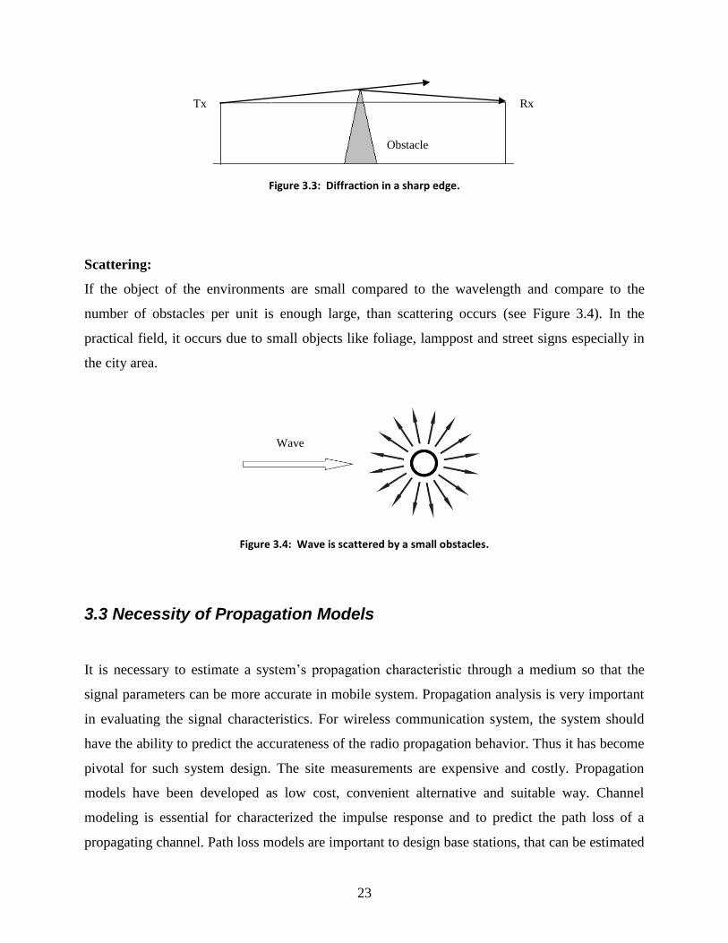
Diffraction is created when the electromagnetic wave propagate from transmitter to receiver

obstructed with a sharp edge surface (see Figure 3.3) [8]. Wave propagates behind the obstacle

when NLOS exist in the radio path, through diffraction. Not only the geometry of the object, but

also the angel of incident, amplitude and phase of the signal also responsible for making

diffraction.

Reflection Refraction

23

Figure 3.3: Diffraction in a sharp edge.

Scattering:

If the object of the environments are small compared to the wavelength and compare to the

number of obstacles per unit is enough large, than scattering occurs (see Figure 3.4). In the

practical field, it occurs due to small objects like foliage, lamppost and street signs especially in

the city area.

Figure 3.4: Wave is scattered by a small obstacles.

3.3 Necessity of Propagation Models

It is necessary to estimate a system‟s propagation characteristic through a medium so that the

signal parameters can be more accurate in mobile system. Propagation analysis is very important

in evaluating the signal characteristics. For wireless communication system, the system should

have the ability to predict the accurateness of the radio propagation behavior. Thus it has become

pivotal for such system design. The site measurements are expensive and costly. Propagation

models have been developed as low cost, convenient alternative and suitable way. Channel

modeling is essential for characterized the impulse response and to predict the path loss of a

propagating channel. Path loss models are important to design base stations, that can be estimated

Wave

Tx Rx

Obstacle

24

us to radiate the transmitter for service of the certain region. Channel characterization deals with

the fidelity of the received signal. The main thing of designing a receiver is to receive the

transmitted signal that has been distorted due to the multipath and dispersion effects of the

channel, and that will receive the transmitted signals. It is very important to have the knowledge

about the electromagnetic environment where the system is operated, and the location of the

transmitter and receiver.

25

CHAPTER 4

Path Loss Models

In our thesis, we analyze five different models which have been proposed by the researchers at

the operating frequency of 3.5 GHz [1-4]. The entire proposed models were investigated by the

developers mostly in European environments. We also choose our parameters for best fitted to

the European environments. In this chapter we consider free space path loss model which is most

commonly used idealistic model. We take it as our reference model; so that it can be realized how

much path loss occurred by the others proposed models.

4.1 Free Space Path Loss Model (FSPL)

Path loss in free space PLFSPL defines how much strength of the signal is lost during propagation

from transmitter to receiver. FSPL is diverse on frequency and distance. The calculation is done

by using the following equation [4]:

(1)

where,

f: Frequency [MHz]

d: Distance between transmitter and receiver [m]

Power is usually expressed in decibels (dBm).

4.2 Okumura Model

The Okumura model [7-8] is a well known classical empirical model to measure the radio signal

strength in build up areas. The model was built by the collected data in Tokyo city in Japan. This

26

model is perfect for using in the cities having dense and tall structure, like Tokyo. While dealing

with areas, the urban area is sub-grouped as big cities and the medium city or normal built cities.

But the area like Tokyo is really big area with high buildings. In Europe, the urban areas are

medium built compared to Tokyo. But in our thesis work, we consider the European cities with

average building heights not more than 15-20 m. Moreover, Okumura gives an illustration of

correction factors for suburban and rural or open areas. By using Okumura model we can predict

path loss in urban, suburban and rural area up to 3 GHz. Our field of studies is 3.5 GHz. We

provided this model as a foundation of Hata-Okumura model.

Median path loss model can be expressed as [7]:

(2)

where

PL: Median path loss [dB]

Lf: Free space path loss [dB]

Amn (f,d): Median attenuation relative to free space [dB]

G (hte): Base station antenna height gain factor [dB]

G (hre): Mobile station antenna height gain factor [dB]

GAREA: Gain due to the type of environment [dB]

and parameters

f: Frequency [MHz]

hte: Transmitter antenna height [m]

hre: Receiver antenna height [m]

d: Distance between transmitter and receiver antenna [km]

Attenuation and gain terms are given in [7]:

27

(3)

The following Figure 3.1 provides the values of Amn(f,d) and GAREA (from set of curves).

Figure 3.1: Median attenuation and area gain factor [8].

4.3 COST 231 Hata Model

The Hata model [6] is introduced as a mathematical expression to mitigate the best fit of the

graphical data provided by the classical Okumura model [7]. Hata model is used for the

frequency range of 150 MHz to 1500 MHz to predict the median path loss for the distance d from

transmitter to receiver antenna up to 20 km, and transmitter antenna height is considered 30 m to

200 m and receiver antenna height is 1 m to 10 m. To predict the path loss in the frequency range

1500 MHz to 2000 MHz. COST 231 Hata model is initiated as an extension of Hata model. It is

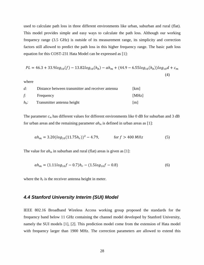
28

used to calculate path loss in three different environments like urban, suburban and rural (flat).

This model provides simple and easy ways to calculate the path loss. Although our working

frequency range (3.5 GHz) is outside of its measurement range, its simplicity and correction

factors still allowed to predict the path loss in this higher frequency range. The basic path loss

equation for this COST-231 Hata Model can be expressed as [1]:

(4)

where


f: Frequency [MHz]

hb: Transmitter antenna height [m]

The parameter cm has different values for different environments like 0 dB for suburban and 3 dB

for urban areas and the remaining parameter ahm is defined in urban areas as [1]:

(5)

The value for ahm in suburban and rural (flat) areas is given as [1]:

(6)

where the hr is the receiver antenna height in meter.

4.4 Stanford University Interim (SUI) Model

IEEE 802.16 Broadband Wireless Access working group proposed the standards for the

frequency band below 11 GHz containing the channel model developed by Stanford University,

namely the SUI models [1], [2]. This prediction model come from the extension of Hata model

with frequency larger than 1900 MHz. The correction parameters are allowed to extend this

29

model up to 3.5 GHz band. In the USA, this model is defined for the Multipoint Microwave

Distribution System (MMDS) for the frequency band from 2.5 GHz to 2.7 GHz [1].

The base station antenna height of SUI model can be used from 10 m to 80 m. Receiver antenna

height is from 2 m to 10 m. The cell radius is from 0.1 km to 8 km [2]. The SUI model describes

three types of terrain, they are terrain A, terrain B and terrain C. There is no declaration about any

particular environment. Terrain A can be used for hilly areas with moderate or very dense

vegetation. This terrain presents the highest path loss. In our thesis, we consider terrain A as a

dense populated urban area. Terrain B is characterized for the hilly terrains with rare vegetation,

or flat terrains with moderate or heavy tree densities. This is the intermediate path loss scheme.

We consider this model for suburban environment. Terrain C is suitable for flat terrains or rural

with light vegetation, here path loss is minimum.

The basic path loss expression of The SUI model with correction factors is presented as [1]:

(7)

where the parameters are

d : Distance between BS and receiving antenna [m]

0d : 100 [m]

: Wavelength [m]

fX : Correction for frequency above 2 GHz [MHz]

hX : Correction for receiving antenna height [m]

s : Correction for shadowing [dB]

: Path loss exponent

The random variables are taken through a statistical procedure as the path loss exponent γ and the

weak fading standard deviation s is defined.

The log normally distributed factor s, for shadow fading because of trees and other clutter on a

propagations path and its value is between 8.2 dB and 10.6 dB [1].

30

The parameter A is defined as [1], [2]:

(8)

and the path loss exponent γ is given by [1]:

(9)

where, the parameter hb is the base station antenna height in meters. This is between 10 m and 80

m. The constants a, b, and c depend upon the types of terrain, that are given in Table 4.1. The

value of parameter γ = 2 for free space propagation in an urban area, 3 < γ < 5 for urban NLOS

environment, and γ > 5 for indoor propagation [2].

Table 4.1: The parameter values of different terrain for SUI model.

Model Parameter Terrain A Terrain B Terrain C

a 4.6 4.0 3.6

b (m-1

) 0.0075 0.0065 0.005

c (m) 12.6 17.1 20

The frequency correction factor Xf and the correction for receiver antenna height Xh for the

model are expressed in [1]:

(10)

(11)

31

where, f is the operating frequency in MHz, and hr is the receiver antenna height in meter. For the

above correction factors this model is extensively used for the path loss prediction of all three

types of terrain in rural, urban and suburban environments.

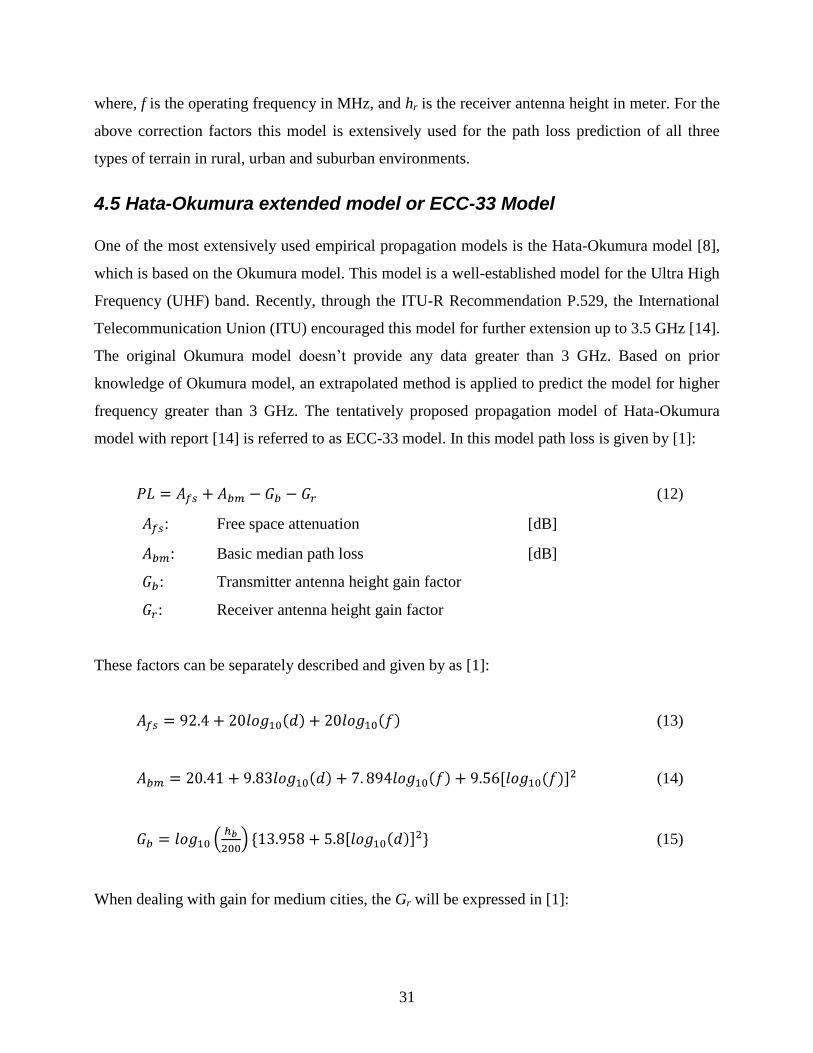
4.5 Hata-Okumura extended model or ECC-33 Model

One of the most extensively used empirical propagation models is the Hata-Okumura model [8],

which is based on the Okumura model. This model is a well-established model for the Ultra High

Frequency (UHF) band. Recently, through the ITU-R Recommendation P.529, the International

Telecommunication Union (ITU) encouraged this model for further extension up to 3.5 GHz [14].

The original Okumura model doesn‟t provide any data greater than 3 GHz. Based on prior

knowledge of Okumura model, an extrapolated method is applied to predict the model for higher

frequency greater than 3 GHz. The tentatively proposed propagation model of Hata-Okumura

model with report [14] is referred to as ECC-33 model. In this model path loss is given by [1]:

(12)

: Free space attenuation [dB]

: Basic median path loss [dB]

: Transmitter antenna height gain factor

: Receiver antenna height gain factor

These factors can be separately described and given by as [1]:

(13)

(14)

(15)

When dealing with gain for medium cities, the Gr will be expressed in [1]:

32

(16)

for large city

(17)

where


f: Frequency [GHz]

hb: Transmitter antenna height [m]

hr: Receiver antenna height [m]

This model is the hierarchy of Okumura-Hata model. So the urban area is also subdivided into

„large city‟ and „medium sized city‟, as the model was formed in the Tokyo city having crowded

and tallest buildings. In our analysis, we consider the medium city model is appropriate for

European cities.

4.6 COST 231 Walfish-Ikegami (W-I) Model

This model is a combination of J. Walfish and F. Ikegami model. The COST 231 project further

developed this model. Now it is known as a COST 231 Walfish-Ikegami (W-I) model. This

model is most suitable for flat suburban and urban areas that have uniform building height (see

Figure 3.2). Among other models like the Hata model, COST 231 W-I model gives a more

precise path loss. This is as a result of the additional parameters introduced which characterized

the different environments. It distinguishes different terrain with different proposed parameters.

The equation of the proposed model is expressed in [4]:

For LOS condition

(18)

33

and for NLOS condition

(19)

where

LFSL= Free space loss

Lrts= Roof top to street diffraction

Lmsd= Multi-screen diffraction loss

Figure 3.2: Diffraction angel and urban scenario.

free space loss [4]:

(20)

roof top to street diffraction (see Figure 3.2) [4]:

hroof hmobile

(24)

34

where

(21)

Note that

The multi-screen diffraction loss is [4]:

(22)

where

(23)

(24)

(25)

(26)

where

35

d: Distance between transmitter and receiver antenna [m]

f: Frequency [GHz]

B: Building to building distance [m]

w: Street width [m]

: Street orientation angel w.r.t. direct radio path [degree]

In our simulation we use the following data, i.e. building to building distance 50 m, street width

25 m, street orientation angel 30 degree in urban area and 40 degree in suburban area and average

building height 15 m, base station height 30 m.

4.7 Ericsson Model

To predict the path loss, the network planning engineers are used a software provided by Ericsson

company is called Ericsson model [2]. This model also stands on the modified Okumura-Hata

model to allow room for changing in parameters according to the propagation environment. Path

loss according to this model is given by [2]:

(27)

where is defined by [2]:

(28)

and parameters

f: Frequency [MHz]

hb: Transmission antenna height [m]

hr: Receiver antenna height [m]

The default values of these parameters (a0, a1, a2 and a3) for different terrain are given in Table

4.2

36

Table 4.2: Values of parameters for Ericsson model [2], [18].

Environment a0 a1 a2 a3

Urban 36.2 30.2 12.0 0.1

Suburban 43.20* 68.93* 12.0 0.1

Rural 45.95* 100.6* 12.0 0.1

*The value of parameter a0 and a1 in suburban and rural area are based on the Least Square (LS)

method in [18].

37

CHAPTER 5

Simulation of Models

In our computation, we fixed our operating frequency at 3.5 GHz; distance between transmitter

antenna and receiver antenna is 5 km, transmitter antenna height is 30 m in urban and suburban

area and 20 m in rural area. We considered 3 different antenna heights for receiver i.e. 3 m, 6 m

and 10 m. As we deemed European environment, we fixed 15 m average building height and

building to building distance is 50 m and street width is 25 m. Most of the models provide two

different conditions i.e. LOS and NLOS. In our entire thesis we concentrate on NLOS condition

except in rural area, we consider LOS condition for COST 231 W-I model, because COST 231

W-I model did not provide any specific parameters for rural area. We exploited Free Space

Model (FSL) as a reference model in our whole comparisons. The following Table 5.1 presents

the parameters we applied in our simulation.

Table 5.1: Simulation parameters

Parameters Values

Base station transmitter power 43 dBm

Mobile transmitter power 30 dBm

Transmitter antenna height 30 m in urban and suburban and

20 m in rural area

Receiver antenna height 3 m, 6 m and 10 m

Operating frequency 3.5 GHz

Distance between Tx-Rx 5 km

Building to building distance 50 m

Average building height 15 m

Street width 25 m

Street orientation angle 300 in urban and 40

0 in suburban

Correction for shadowing 8.2 dB in suburban and rural and

10.6 dB in urban area

38

5.1 Path loss in urban area

In our calculation, we set 3 different antenna heights (i.e. 3 m, 6 m and 10 m) for receiver,

distance varies from 250 m to 5 km and transmitter antenna height is 30 m. The numerical results

for different models in urban area for different receiver antenna heights are shown in the Figure

5.1, 5.2 and 5.3.

Figure 5.1: Path loss in urban environment at 3 m receiver antenna height.

0 0.5 1 1.5 2 2.5 3 3.5 4 4.5 590

100

110

120

130

140

150

160

170

180

190

Distance between Tx and Rx (km)

Path

loss (

dB

)

3 m receiver antenna height in urban environment

COST WIFSPLECC-33

COST HataSUIEricsson

39



0 0.5 1 1.5 2 2.5 3 3.5 4 4.5 590

100

110

120

130

140

150

160

170

180


Path

loss (

dB

)


COST WI

FSPL

ECC-33COST Hata

SUI

Ericsson

0 0.5 1 1.5 2 2.5 3 3.5 4 4.5 590

100

110

120

130

140

150

160

170


Path

loss (

dB

)


COST WI

FSPL

ECC-33

COST Hata

SUI

Ericsson

40

Table 5.2 summarized the path loss data at 2 km Tx-Rx distance in urban environment. Path loss

is varied according to the changes of receiver antenna height.

Table 5.2: Path loss estimate at 2 km distance in urban environment

Propagation

Models

Transmitter

antenna height

(m)

Transmitter

power

(dBm)

Path loss (dB) at

3 m receiver

antenna height

Path loss (dB) at

6 m receiver

antenna height

Path loss (dB) at

10 m receiver

antenna height

Free Space Loss 30 43 110 110 110

ECC-33 30 43 167 152 141

COST 231 Hata 30 43 157 154 150

Ericsson 30 43 142 140 138

SUI 30 43 154 148 144

COST 231 W-I 30 43 159 156 151

41

5.2 Path loss in suburban area

The transmitter and receiver antenna heights are same as used earlier. The numerical results for

different models in suburban area for different receiver antenna heights are shown in Figure 5.4,

5.5 and 5.6.

Figure 5.4: Path loss in suburban environment at 3 m receiver antenna height.

0 0.5 1 1.5 2 2.5 3 3.5 4 4.5 580

100

120

140

160

180

200


Path

loss (

dB

)

3 m receiver antenna height in suburban environment

COST WI

FSPL

ECC-33

COST Hata

SUI

Ericsson

42



0 0.5 1 1.5 2 2.5 3 3.5 4 4.5 560

80

100

120

140

160

180

200


Path

loss (

dB

)


COST WI

FSPL

ECC-33

COST Hata

SUI

Ericsson

0 0.5 1 1.5 2 2.5 3 3.5 4 4.5 560

80

100

120

140

160

180

200


Path

loss (

dB

)


COST WIFSPL

ECC-33COST Hata

SUIEricsson

43



Table 5.3: Path loss estimate at 2 km distance in suburban environment

Propagation

Models

Transmitter

antenna height

(m)

Transmitter

power

(dBm)

Path loss (dB) at

3 m receiver

antenna height

Path loss (dB) at

6 m receiver

antenna height

Path loss (dB) at

10 m receiver

antenna height

Free space model 30 43 110 110 110

ECC-33 30 43 167 152 141

COST 231 Hata 30 43 152 142 130

Ericsson 30 43 160 157 156

SUI 30 43 121 118 115

COST 231 W-I 30 43 147 145 140

44

5.3 Path loss in rural area

The receiver antenna heights are same as used earlier. Here we considered 20 m for transmitter

antenna height. The ECC-33 model is not applicable in rural area and the COST 231 W-I model

has no specific parameters for rural area, we consider LOS equation provided by this model. The

numerical results for different models in rural area for different receiver antenna heights are

shown in Figure 5.7, 5.8 and 5.9.

Figure 5.7: Path loss in rural environment at 3 m receiver antenna height.

0 0.5 1 1.5 2 2.5 3 3.5 4 4.5 580

100

120

140

160

180

200

220


Path

loss (

dB

)

3 m receiver antenna height in rural environment

COST WI

FSPL

COST Hata

SUI

Ericsson

45



0 0.5 1 1.5 2 2.5 3 3.5 4 4.5 580

100

120

140

160

180

200

220


Path

loss (

dB

)


COST WI

ECC-33

COST Hata

SUI

Ericsson

0 0.5 1 1.5 2 2.5 3 3.5 4 4.5 580

100

120

140

160

180

200

220


Path

loss (

dB

)


COST WIFSPLCOST HataSUIEricsson

46



Table 5.4: Path loss estimate at 2 km distance in rural environment

Propagation

Models

Transmitter

antenna height

(m)

Transmitter

power

(dBm)

Path loss (dB) at

3 m receiver

antenna height

Path loss (dB) at

6 m receiver

antenna height

Path loss (dB) at

10 m receiver

antenna height

Free space model 20 43 110 110 110

ECC-33 20 43 Not applicable Not applicable Not applicable

COST 231 Hata 20 43 154 145 132

Ericsson 20 43 175 173 171

SUI 20 43 148 142 138

COST 231 W-I 20 43 121 121 121

47

CHAPTER 6

Analysis of simulation results in urban area

The accumulated results for urban environment are shown in Figure 6.1. Note that Ericsson

model showed the lowest prediction (142 dB to 138 dB) in urban environment. It also showed the

lowest fluctuations compare to other models when we changed the receiver antenna heights. In

that case, the ECC-33 model showed the heights path loss (167 dB) and also showed huge

fluctuations due to change of receiver antenna height. In this model, path loss is decreased when

increased the receiver antenna height. Increase the receiver antenna heights will provide the more

probability to find the better quality signal from the transmitter. COST 231 W-I model showed

the biggest path loss at 10 m receiver antenna height. But this model is considered for precise

analysis due to additional parameters which described some environmental characteristics.

Figure 6.1: Analysis of simulation results for urban environment in different receiver antenna height.

ECC-33 COST-Hata Ericsson SUI COST-WI

Rx height 3m 167 157 142 156 159

Rx height 6m 152 154 140 148 156

Rx height 10m 141 150 138 144 151

167157

142156 159152 154

140148

156141

150138 144 151

0

20

40

60

80

100

120

140

160

180

Pat

h lo

ss (

dB

)

distance at 2 km

Urban Environment

48

Analysis of simulation results in suburban area

The accumulated results for suburban environment are shown in Figure 6.2. In following chart, it

showed that the SUI model predict the lowest path loss (121 dB to 115 dB) in this terrain with

little bit flections at changes of receiver antenna heights. Ericsson model showed the heights path

loss (157 dB and 156 dB) prediction especially at 6 m and 10 m receiver antenna height. The

COST-Hata model showed the moderate result with remarkable fluctuations of path loss with-

respect-to antenna heights changes. The ECC-33 model showed the same path loss as like as

urban environment because of same parameters are used in the simulation.

Figure 6.2: Analysis of simulation results for suburban environment in different receiver antenna height.


Rx height 3m 167 152 160 121 147

Rx height 6m 152 142 157 118 145

Rx height 10m 141 130 156 115 140

167152

160

121

147152142

157

118

145141130

156

115

140

0

20

40

60

80

100

120

140

160

180

Pat

h lo

ss (

dB

)

distance at 2 km

Suburban Environment

49

Analysis of simulation results in rural area

The accumulated results for rural environment are shown in Figure 6.3. In this environment

COST 231 Hata model showed the lowest path loss (129 dB) prediction especially in 10 m

receiver antenna height and also showed significant fluctuations due to change the receiver

antenna heights. COST 231 W-I model showed the flat results in all changes of receiver antenna

heights. There are no specific parameters for rural area. In our simulation, we considered LOS

equation for this environment (the reason is we can expect line of sight signal if the area is flat

enough with less vegetations). Ericsson model showed the heights path loss (173 dB to 168 dB)

which is remarkable, may be the reason is the value of parameters a0 and a1 are extracted by the

LS methods [18].

Figure 6.3: Analysis of simulation results for rural environment in different receiver antenna height.


Rx height 3m 0 152 173 143 121

Rx height 6m 0 142 170 137 121

Rx height 10m 0 129 168 133 121

0

152

173

143

121

0

142

170

137121

0

129

168

133121

0

20

40

60

80

100

120

140

160

180

200

Pat

h lo

ss (

dB

)

distance at 2 km

Rural Environment

50

CHAPTER 7

Conclusions

Our comparative analysis indicate that due to multipath and NLOS environment in urban area, all

models experiences higher path losses compare to suburban and rural areas. Moreover, we did

not find any single model that can be recommended for all environments.

We can see in urban area (data shown in Figure 6.1), the Ericsson model showed the lowest path

loss (138 dB in 10 m receiver antenna height) as compared to other models. Alternatively, the

ECC-33 model showed the heights path loss (167 dB in 3 m receiver antenna height).

In suburban area (data shown in Figure 6.2) the SUI model showed quite less path loss (115 dB)

compared to other models. On the other hand, ECC-33 model showed heights path loss as

showed in urban area. Moreover, Ericsson model showed remarkable higher path loss for 6 m and

10 m receiver antenna heights (i.e.157 dB and 156 dB respectively).

In rural area (data shown in Figure 6.3), we can choose different models for different

perspectives. If the area is flat enough with less vegetation, where the LOS signal probability is

high, in that case, we may consider LOS calculation. Alternatively, if there is less probability to

get LOS signal, in that situation, we can see COST-Hata model showed the less path loss (129

dB) compare to SUI model (133 dB) and Ericsson model (168 dB) especially in 10 m receiver

antenna height. But considering all receiver antenna heights SUI model showed less path loss

(143 dB in 3 m and 137 dB in 6 m) whereas COST-Hata showed higher path loss (152 dB in 3m

and 142 dB in 6 m).

If we consider the worst case scenario for deploying a coverage area, we can serve the maximum

coverage by using more transmission power, but it will increase the probability of interference

with the adjacent area with the same frequency blocks. On the other hand, if we consider less

path loss model for deploying a cellular region, it may be inadequate to serve the whole coverage

51

area. Some users may be out of signal in the operating cell especially during mobile condition.

So, we have to trade-off between transmission power and adjacent frequency blocks interference

while choosing a path loss model for initial deployment.

Future work

In future, our simulated results can be tested and verified in practical field. We may also derive a

suitable path loss model for all terrain. Future study can be made for finding more suitable

parameters for Ericsson and COST 231 W-I models in rural area.

52

APPENDICES

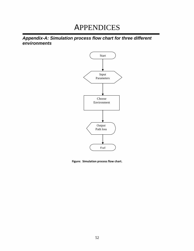
Appendix-A: Simulation process flow chart for three different environments

Figure: Simulation process flow chart.

Input

Parameters

Choose

Environment

End

Output

Path loss

Start

53

Appendix-B: MATLAB Code for Urban environment in different antenna heights

%%%%%%%%%%%%%% models for urban area in 10/6/3 m receiver antenna height%%%%% close all; clear all; clc %Distance in Kilometer N=5; d=0.0:0.25:N; %frequency in MHz f=3500; %transmitter antenna heights 30 m hb=30; %receiver antenna heights 10/6/3 m hr=10; %%%%%%%%%%%%%%%%Free Space Loss%%%%%%%%%%%%%%%%%%%

fsmodel=32.45+20.*log10(d)+20.*log10(f);

%%%%%%%%%%%%%%% COST 231 W I model%%%%%%%%%%%%%%

%distance between buildings B=50; %street width B/2 w=25; %Hmobile=h roof-h mobile(15-10)m we consider h roof is 15 m Hmobile=5; %street orientation angel 30 degree theta=30; Lori=-10+0.354*theta; Lrts=-16.9-10.*log10(w)+10.*log10(f)+20.*log10(Hmobile)+Lori; Lfs=32.45+20.*log10(d)+20.*log10(f); %Hbase=h base-h roof(30-15)we cosider transmitter height is 30 m Hbase=15; Lmsd=-18.*log10(1+Hbase)+54+18.*log10(d)+(-4+1.5*((f/925)-1)).*log10(f)-

9.*log10(B); PLcwi=Lfs+Lrts+Lmsd;

%%%%%%%%%%%%%%%%ECC-33 Model %%%%%%%%%%%%

y=log10(hr)-0.585; %frequency in GHz f=3.5; Afs=92.4+20.*log10(d)+20.*log10(f); Abm=20.41+9.83.*log10(d)+7.894.*log10(f)+9.56*2.*log10(f); %in urban environment the parameter a=3.6,b=0.005,c=20 in m a=(5.8*2*(log10(d))); b=13.958; c=log10(hb/200); Gb=c.*(b+a); x=42.57+13.7.*log10(f); Gr=x.*y; PLecc=Afs+Abm-Gb-Gr;

54

%%%%%%%%%%%%%%%%%Cost 231 hata Model%%%%%%%%%%%%%%%

%frequency in MHz f=3500; %3dB in urban area cm=3; ahm2=3.20.*(log10(11.75*hr))^2-4.97; PLch=46.3+33.9.*log10(f)-13.82.*log10(hb)-ahm2+(44.9-

6.55.*log10(hb))*log10(d)+cm;

%%%%%%%%%%%%%%%%SUI model%%%%%%%%%%%

%100 m used as a reference d1= 0.1; %receiver hight lambda=((3*10^8)/( 3500*10^6)); % frequency in MHz f=3500; %fading standard deviation s is 10.6 dB in urban s=10.6; a=3.6; b=0.005; c=20; gamma=a-b*hb+c/hb; PLsui=20.*log10((4*pi*d1)/lambda)+10*gamma.*log10(d/d1)+6.*log10(f/2000)-

20.*log10(hr/2000)+s;

%%%%%%%%%%%%%%%%%% Ericsson Model 9999 %%%%%%%%%%%%%%%%%%%%%

g(f)=44.49.*log10(f)-9.56.*log10(f); PL9999=36.2+30.2.*log10(d)-12.*log10(hb)+0.1.*log10(hb)*log10(d)-

6.4.*log10(11.75*hr)+g(f);

%%%%%%%%%%%%%%%%%Plotting%%%%%%%%%%%%%%%%%%%%%%

plot(d,PLcwi, 'b+-',d,fsmodel,'ks',d,PLecc, 'r*-',d,PLch,'g.-',d,PLsui,'k.-

',d,PL9999,'m.-'); grid on;

%%%%%%%%%%%%%%%%%Axis and Title%%%%%%%%%%%%%%%%%%%

xlabel('Distance between Tx and Rx (km)'); ylabel('Path loss (dB)'); title('10 m receiver antenna height in urban environment')

55

Appendix-C: MATLAB Code for Suburban environment in different antenna heights

%%%%%%%%%%%%% models for suburban area in 10/6/3 m receiver antenna

height%%%%% close all; clear all; clc %Distance in Kilometer N=5; d=0.0:0.25:N; %frequency in MHz f=3500; %transmitter antenna heights 30 m hb=30; %receiver antenna heights 10/6/3 m hr=10; %%%%%%%%%%%%%%%%Free Space Loss%%%%%%%%%%%%%%%%%%%


%%%%%%%%%%%%%%% COST 231 W I model%%%%%%%%%%%%%%

%distance between buildings B=50; %street width B/2 w=25; %Hmobile=h roof-h mobile(15-10/6/3)m we consider h roof is 15 m Hmobile=5; %street orientation angel 40 degree theta=40; Lori=2.5+0.075*(theta-35); Lrts=-16.9-10.*log10(w)+10.*log10(f)+20.*log10(Hmobile)+Lori; Lfs=32.45+20.*log10(d)+20.*log10(f); %Hbase=h base-h roof(30-15)we cosider transmitter height is 30 m Hbase=15; %in suburban kf is (-4+.07((f/925)-1)) Lmsd=-18.*log10(1+Hbase)+54+18.*log10(d)+(-4+0.07*((f/925)-1)).*log10(f)-

9.*log10(B); PLcwi=Lfs+Lrts+Lmsd;

%%%%%%%%%%%%%%%%ECC-33 Model for %%%%%%%%%%%%

y=log10(hr)-0.585; %frequency in GHz f=3.5; Afs=92.4+20.*log10(d)+20.*log10(f); Abm=20.41+9.83.*log10(d)+7.894.*log10(f)+9.56*2.*log10(f); %in urban environment the parameter a=3.6,b=0.005,c=20 in m a=(5.8*2*(log10(d))); b=13.958; c=log10(hb/200); Gb=c.*(b+a); x=42.57+13.7.*log10(f);

56

Gr=x.*y; PLecc=Afs+Abm-Gb-Gr;

%%%%%%%%%%%%%%%%%Cost 231 hata Model%%%%%%%%%%%%%%%

%frequency in MHz f=3500; %0dB in suburban area cm=0; ahm=(1.11.*log10(f)-0.7)*hr-(1.5.*log10(f)-0.8) PLch=46.3+33.9.*log10(f)-13.82.*log10(hb)-ahm+(44.9-

6.55.*log10(hb))*log10(d)+cm;

%%%%%%%%%%%%%%%%SUI model%%%%%%%%%%%

%100 m is used as a reference in SUI model d1= 0.1; %receiver hight lambda=((3*10^8)/( 3500*10^6)); % frequency in MHz f=3500; %fading standard deviation s is 8.2 dB in suburban s=8.2; % Suburban is consider as a terrain B a=4; b=0.0065; c=17.1; gamma=a-b*hb+c/hb; PLsui=20.*log10((4*pi*d1)/lambda)+10*gamma.*log10(d/d1)+6.*log10(f/2000)-

10.8.*log10(hr/2000)+s; %%%%%%%%%%%%%%%%%% Ericsson Model 9999 %%%%%%%%%%%%%%%%%%%%%

g(f)=44.49.*log10(f)-9.56.*log10(f); PL9999=43.20+68.93.*log10(d)-12.*log10(hb)+0.1.*log10(hb)*log10(d)-

6.4.*log10(11.75*hr)+g(f);

%%%%%%%%%%%%%%%%%Plotting%%%%%%%%%%%%%%%%%%%%%%

plot(d,PLcwi, 'b+-',d,fsmodel,'ks',d,PLecc, 'r*-',d,PLch,'g.-',d,PLsui,'k.-

',d,PL9999,'m.-'); grid on;

%%%%%%%%%%%%%%%%%Axis and Title%%%%%%%%%%%%%%%%%%%

xlabel('Distance between Tx and Rx (km)'); ylabel('Path loss (dB)'); title('10 m receiver antenna height in suburban environment');

57

Appendix-D: MATLAB Code for rural environment in different antenna heights

%%%%%%%%%%%%%% models for rural area in 10/6/3 m receiver antenna height%%%%% close all; clear all; clc %Distance in Kilometer N=5; d=0.0:0.25:N; %frequency in MHz f=3500; %transmitter antenna heights 20 m in rural area hb=20; %receiver antenna heights 10/6/3 m hr=10; %%%%%%%%%%%%%%%%Free Space Loss%%%%%%%%%%%%%%%%%%%


%%%%%%%%%%%%%%% COST 231 W I model%%%%%%%%%%%%%% % we consider LOS equation for rural PLcwi=42.6+26.*log10(d)+20.*log10(f);

%%%%%%%%%%%%%%%%ECC-33 Model%%%%%%%%%%%% %%%%%%%% not applicable in rural area%%%%% %%%%%%%%%%%%%%%%%Cost 231 hata Model%%%%%%%%%%%%%%%

%frequency in MHz f=3500; %0dB in rural area cm=0; ahm=(1.11.*log10(f)-0.7)*hr-(1.5.*log10(f)-0.8) PLch=46.3+33.9.*log10(f)-13.82.*log10(hb)-ahm+(44.9-

6.55.*log10(hb))*log10(d)+cm;

%%%%%%%%%%%%%%%%SUI model%%%%%%%%%%%

%100 m used as a reference d1= 0.1; %receiver hight lambda=((3*10^8)/( 3500*10^6)); % frequency in MHz f=3500; %fading standard deviation s is 8.2 dB in rural s=8.2; % Urban is consider as a Terrain A with highest path loss% a=3.6; b=0.005; c=20; gamma=a-b*hb+c/hb; PLsui=20.*log10((4*pi*d1)/lambda)+10*gamma.*log10(d/d1)+6.*log10(f/2000)-

20.*log10(hr/2000)+s;

58

%%%%%%%%%%%%%%%%%% Ericsson Model 9999 %%%%%%%%%%%%%%%%%%%%% g(f)=44.49.*log10(f)-9.56.*log10(f); PL9999=45.95+100.6.*log10(d)-12.*log10(hb)+0.1.*log10(hb)*log10(d)-

6.4.*log10(11.75*hr)+g(f);

%%%%%%%%%%%%%%%%%Plotting%%%%%%%%%%%%%%%%%%%%%% plot(d,PLcwi, 'b+-',d,fsmodel,'ks',d,PLch,'g.-',d,PLsui,'k.-',d,PL9999,'m.-');

grid on;

%%%%%%%%%%%%%%%%%Axis and Title%%%%%%%%%%%%%%%%%%%

xlabel('Distance between Tx and Rx (km)'); ylabel('Path loss (dB)'); title('6 m receiver antenna height in rural environment');

59

Appendix-E: Abbreviations and Acronyms

AAS Advanced Antenna Systems

ACI Aadjacent-Channel Interference

AES Advanced Encryption Standard

AMC Adaptive Modulation and Coding

ARQ Automatic Repeat Request

BPSK Binary Phase Shift Keying

BS Base Station

BWA Broadband Wireless Access

DES Data Encryption Algorithm

ECC Electronic Communication Committee

FDD Frequency Division Duplex

FEC Forward Error Correction

FFT Fast Fourier Transform

FSL Free Space Loss

FWA Fixed Wireless Access

GIS Graphical Information System

GSM Global System for Mobile Communications

ITU International Telecommunication Union

LOS Line-of-Sight

MANs Metropolitan Area Networks

MAC Medium Access Control

MMDS Multipoint Microwave Distribution System

NLOS Non-Line-of-Sight

OFDM Orthogonal Frequency Division Multiplex

OFDMA Orthogonal Frequency Division Multiple Access

PHY Physical

PL Path Loss

QAM Quadrature Amplitude Modulation

QoS Quality of Services

QPSK Quadrature Phase Shift Keying

60

SISP Site Specific

SNR Noise to Signal Ratio

SS Subscribers Station

SUI Stanford University Interim

TDD Time Division Duplex

TDM Time Division Multiplexed

UHF Ultra High Frequency

UMTS Universal Mobile Telecommunication System

VHF Very High Frequency

WI Walfish-Ikegami

WMAN Wireless Metropolitan Area Networks

61

References

[1] V.S. Abhayawardhana, I.J. Wassel, D. Crosby, M.P. Sellers, M.G. Brown, “Comparison of

empirical propagation path loss models for fixed wireless access systems,” 61th

IEEE

Technology Conference, Stockholm, pp. 73-77, 2005.

[2] Josip Milanovic, Rimac-Drlje S, Bejuk K, “Comparison of propagation model accuracy for

WiMAX on 3.5GHz,” 14th

IEEE International conference on electronic circuits and systems,

Morocco, pp. 111-114. 2007.

[3] Joseph Wout, Martens Luc, “Performance evaluation of broadband fixed wireless system

based on IEEE 802.16,” IEEE wireless communications and networking Conference, Las

Vegas, NV, v2, pp.978-983, April 2006.

[4] V. Erceg, K.V. S. Hari, M.S. Smith, D.S. Baum, K.P. Sheikh, C. Tappenden, J.M. Costa, C.

Bushue, A. Sarajedini, R. Schwartz, D. Branlund, T. Kaitz, D. Trinkwon, "Channel Models

for Fixed Wireless Applications," IEEE 802.16 Broadband Wireless Access Working Group,

2001.

[5] http://www.wimax360.com/photo/global-wimax-deployments-by [Accessed: June 28 2009]

[6] M. Hata, “Empirical formula for propagation loss in land mobile radio services,” IEEE

Transactions on Vehicular Technology, vol. VT-29, pp. 317-325, September 1981.

[7] Y.Okumura, “Field strength variability in VHF and UHF land mobile services,” Rev. Elec.

Comm. Lab. Vol. 16, pp. 825-873, Sept-Oct 1968.

[8] T.S Rappaport, Wireless Communications: Principles and Practice, 2n ed. New delhi:

Prentice Hall, 2005 pp. 151-152.

[9] Well known propagation model, [Online]. Available:

http://en.wikipedia.org/wiki/Radio_propagation_model [Accessed: April 11, 2009]

[10] IEEE 802.16 working group, [Online]. Available:

http://en.wikipedia.org/wiki/IEEE_802.16 [Accessed: April 11, 2009]

[11] Jeffrey G Andrews, Arunabha Ghosh, Rias Muhamed, “Fundamentals of WiMAX:

understanding Broadband Wireless Networking”, Prentice Hall, 2007

http://en.wikipedia.org/wiki/IEEE_802.16

62

[12] WiMAX Forum, “Documentation, Technology Whitepapers”, [Online]. Available at

WiMAX Forum.org: http://www.wimaxforum.org/resources/documents [Accessed: April 18,

2008

[13] Doppler spread, [Online]. Available: http://en.wikipedia.org/wiki/Fading [Accessed: April

11, 2009]

[14] Electronic Communication Committee (ECC) within the European Conference of Postal

and Telecommunication Administration (CEPT), “The analysis of the coexistence of FWA

cells in the 3.4 – 3.8 GHz band,” tech. rep., ECC Report 33, May 2003.

[15] Rony Kowalski, “The Benefits of Dynamic Adaptive Modulation for High Capacity

Wireless Backhaul Solutions”, Ceragon Networks, [Online]. Available:

http://www.ceragon.com/files/The%20Benefits%20of%20Dynamic%20Adaptive%20Modula

tion.pdf [Accessed: April 18, 2009].

[16] D. Pareek, The Business of WiMAX, Chapter 2 and Chapter 4, John Wiley, 2006

[17] Empirical Models, [Online] Available: http://en.wikipedia.org/wiki/Empirical_model

[Accessed April 18, 2009]

[18] Simic I. lgor, Stanic I., and Zrnic B., “Minimax LS Algorithm for Automatic Propagation

Model Tuning,” Proceeding of the 9th

Telecommunications Forum (TELFOR 2001),

Belgrade, Nov.2001.

http://en.wikipedia.org/wiki/Fading

http://en.wikipedia.org/wiki/Empirical_model

analysis of propagation models for wimax at 3.5 ghz830403/fulltext01.pdf · okumura model, hata...

Documents