analysis of piezoelectric laminates by generalized finite
TRANSCRIPT

Analysis of piezoelectric laminates by generalized finite element method and mixed layerwise-
HSDT models
This article has been downloaded from IOPscience. Please scroll down to see the full text article.
2010 Smart Mater. Struct. 19 035004
(http://iopscience.iop.org/0964-1726/19/3/035004)
Download details:
IP Address: 150.162.22.35
The article was downloaded on 30/07/2010 at 22:20
Please note that terms and conditions apply.
View the table of contents for this issue, or go to the journal homepage for more
Home Search Collections Journals About Contact us My IOPscience

IOP PUBLISHING SMART MATERIALS AND STRUCTURES
Smart Mater. Struct. 19 (2010) 035004 (13pp) doi:10.1088/0964-1726/19/3/035004
Analysis of piezoelectric laminates bygeneralized finite element method andmixed layerwise-HSDT modelsD A F Torres and P T R Mendonca
Group of Mechanical Analysis and Design—GRANTE, Department of MechanicalEngineering, Federal University of Santa Catarina, 88040-900, Florianopolis, SC, Brazil
E-mail: [email protected] and [email protected]
Received 16 April 2009, in final form 7 December 2009Published 22 January 2010Online at stacks.iop.org/SMS/19/035004
AbstractThis paper presents a procedure to numerically analyze the coupled electro-structural responseof laminated plates with orthotropic fiber reinforced layers and piezoelectric layers using thegeneralized finite element method (GFEM). The mechanical unknowns, the displacements, aremodeled by a higher order shear deformation theory (HSDT) of the third order, involving sevengeneralized displacement functions. The electrical unknowns, the potentials, are modeled by alayerwise theory, utilizing piecewise linear functions along the thickness of the piezoelectriclayers. All fields are enriched in the in-plane domain of the laminate, according to the GFEM,utilizing polynomial enrichment functions, defined in global coordinates, applied on a bilinearpartition of unities defined on each element. The formulation is developed from an extendedprinciple of Hamilton and results in a standard discrete algebraic linear motion equation.Numerical results are obtained for some static cases and are compared with several numericaland experimental results published in the literature. These comparisons show consistent andreliable responses from the formulation. In addition, the results show that GFEM meshesrequire the least number of elements and nodes possible for the distribution of piezoelectricpatches and the enrichment provides more flexibility to reproduce the deformed shapes ofadaptive laminated plates.
1. Introduction
Smart/intelligent structures have received increasing attentionfrom researchers in recent decades due to several aspects.The motivation for utilizing adaptive materials is to enablea structure to change its shape or its material/structuralproperties, thereby improving performance and service life.
Electrostrictive materials, magnetostrictive materials,shape memory alloys, magneto- or electro-rheological fluids,polymer gels, and piezoelectric materials, for example, can allbe used to design and develop structures that can be calledsmart.
These adaptive materials can reduce the need for complexmechanical linkages and actuator systems since the adaptivematerial itself is integrated (embedded/bonded) within thestructure, resulting in the reduction of weight and avoidingsome problems inherent to these mechanical devices (Cheeet al 1998).
Piezoelectric materials can be applied in laminatedcomposite structures as patches and films or to formlayers within of the laminate. Because they exhibitcoupled mechanical–electrical behavior, they can be used assensors, measuring strains and accelerations, or as actuators,when electric potentials are applied to generate a field ofdeformations in the structure.
In the past three decades, a large variety of modelshave been developed to predict the behavior of piezoelectricmaterials in smart structures. These models may beclassified into three different categories: induced strain models,coupled electromechanical models and coupled thermo-electromechanical models.
The coupled electromechanical models provide a moreconsistent representation of both the active and sensitiveresponses of piezoelectric materials through the incorporationof both mechanical displacements and electric potentialsas state variables in the formulation. The coupled
0964-1726/10/035004+13$30.00 © 2010 IOP Publishing Ltd Printed in the UK1

Smart Mater. Struct. 19 (2010) 035004 D A F Torres and P T R Mendonca
electromechanical models are most commonly implemented infinite element codes. The early codes were modeled with solidelements, following the pioneering work of Allik and Hughes(1970). However, the hexahedron or brick elements displayexcessive shear stiffness as the element thickness decreases.This problem was circumvented by adding three incompatibleinternal degrees of freedom to the element (Detwiler et al1995). Other formulations based on solid elements havebeen developed, (see, for instance, Tzou and Tseng (1990)and Ha et al (1992)), but, as a rule, the completely three-dimensional modeling of laminated piezoelectric structuresresults in systems with a large number of degrees of freedom,since they require one solid element per layer of the laminate.
One strategy to reduce the cost associated with the fullsolid element models is in the use of a layerwise theory (LT)to describe both mechanical and electrical unknowns. Amongothers, Saravanos et al (1997) can be cited as a reference forthe complete dynamic electromechanical response of smartpiezoelectric plates under external mechanical or electricloading. Lee (2001) presents a complete family of finiteelements for beams, plates and shells based on LT for all statevariables. Lage et al (2004), also incorporated the coupledmagneto-electro-elastic phenomenon in a partially hybridfunctional with higher order functions along the thickness. Amore elaborate strategy is developed by Cotoni et al (2006),who presents a finite element formulation based on a fourthorder expansion through the laminate thickness, combined witha piecewise linear term to describe the mechanical variablesand a quadratic distribution of the electric potential inside eachpiezoelectric layer.
The layerwise theories still involve a large number ofdegrees of freedom in the models, similar in extent to thefull solid elements. This inconvenience induced the paralleldevelopment of two-dimensional models. The most simpleof these are based on the classical laminated plate theory(CLPT), for instance, the work of Hwang and Park (1993),who developed a two-dimensional quadrilateral plate elementwith one electrical degree of freedom per piezoelectric layerper element. The output voltage was post-processed from thedirect piezoelectric equation.
The simple CLPT offers poor kinematic approximationcapabilities for a complex laminate system, such as thoseequipped with piezoelectric patches. Therefore, models basedon the first order shear deformation theory (FSDT) were tested,such as that described by Detwiler et al (1995), for the linearresponse of coupled electrical-mechanical behavior, or by Gaoand Shen (2003), who considered the geometrical non-linearityof the structure.
The particular structural configuration of a laminate withpiezoelectric layers or patches makes it very difficult toadequately model using a single equivalent layer kinematicmodel, applied to both mechanical and electrical unknowns.Therefore, a sensible strategy involves the use of a singleequivalent layer model for the mechanical unknowns and alayerwise theory for the electric potential. Some of the mostsimple of these combinations are those using the FSDT forthe mechanical displacements and LT for the potential, forexample, the shell element formulated by Saravanos (1997).
Cen et al (2002) have also employed a partially hybrid energyfunctional for correcting the transverse shear deformation intheir mixed FSDT–LT finite element formulation. In a differentmanner, Liew et al (2004) utilized the mixed FSDT–LT modelsin a formulation based on the element-free Galerkin method.
It is well known that the FSDT results in some deficienciesin the approximation of the mechanical response of anisotropiclaminates, particularly in the form of underestimateddisplacements and poor transverse shear stresses. A higherorder shear deformation theory (HSDT) behaves much betterand several studies indicate that it is a good choice forthe mechanical displacements in an piezoelectric laminate,combined with the LT for the electric potential. This can beseen in the work of Reddy (1999), Chee (2000) and Faria(2006), among others.
This paper presents a procedure to numerically analyzethe coupled electro-structural response of laminated plateswith orthotropic fiber reinforced layers and piezoelectriclayers, by the generalized finite element method (GFEM).The mechanical unknowns, the displacements, are modeledby an HSDT of the third order. The electrical unknowns,the potentials, are modeled by a layerwise theory, utilizingpiecewise linear functions along the thickness of thepiezoelectric layers. All fields are enriched according to theGFEM, utilizing polynomial enrichment functions applied ona bilinear partition of unity defined on each element. Theremainder of this paper is outlined as follows: section 2reviews the basics of GFEM. Section 3 deals with thelinear electro-elasticity formulation. Section 4 details theproposed application of the GFEM strategy to the problem oflaminated plates with orthotropic piezoelectric layers, showingthe discretization, the global enrichment of the approximatingspaces, stiffness and inertia matrices, mechanical–electricalcoupling matrices and mechanical and electric dynamic loadvectors. Section 5 shows numerical applications for the staticanalysis of classical models of adaptive plates comparing theresults of the present formulation with those in the literature,and section 6 gives some conclusions.
2. Generalized finite element method
Oden et al (1998) presented a hybrid method combiningthe hp clouds method and the conventional form of thefinite element method. This strategy takes into account theidea of adding hierarchical refinements to a set of shapefunctions associated to finite elements, such as the Lagrangianinterpolation functions which satisfy the requirement of apartition of unity (PoU). The method became consolidated withthe works of Duarte et al (2000), Strouboulis et al (2000) andStrouboulis et al (2001), resulting in the methodology calledgeneralized finite element method (GFEM).
In the GFEM context, discrete spaces for a Galerkinmethod are defined using the concept of the partition of unitfinite element method (PUFEM), of Babuska et al (1994),Melenk (1995), Melenk and Babuska (1996), and Babuskaand Melenk (1997) and of the hp clouds method of Duarte(1996) and Duarte and Oden (1996). A mesh of elementsis created to: (a) facilitate the numerical integration; and (b)
2

Smart Mater. Struct. 19 (2010) 035004 D A F Torres and P T R Mendonca
define the PoU locally within elements by intrinsic coordinates.Finally, the PoU functions are enriched by functions defined inglobal coordinates. This last aspect is responsible for the highefficiency of the method. Usually the enrichment functions arepolynomials, but special enrichment functions can be used toprovide more accurate and robust simulations. These functionscan be built based on a priori knowledge of the solution ofa problem as well as based on the solution of local boundaryvalue problems.
In recent years, the GFEM has been applied to adiversity of phenomena such as the analysis of dynamiccrack propagation (Duarte et al 2001) and porous materials(Strouboulis et al 2001, 2003). It has also been used tobuild arbitrarily smooth approximations for handling higherorder distributional boundary conditions (Duarte et al 2006).Barros et al (2007) uses it to perform p-adaptive analysis anderror estimation. O’Hara (2007) and O’Hara et al (2009)use GFEM to analyze multiscale phenomena. Barcellos et al(2009) develops a Ck continuous finite element formulation forthe Kirchhoff laminate model. A procedure to define richerapproximate subspaces for shell structures and the treatmentof the boundary layer phenomenon is addressed by Garcia et al(2009).
Partition of unity (PoU) is a set of functions where, amongother properties (see Oden and Reddy 1976), the sum of theirvalues is equal to unity on every point of the support. It canbe noted that the standard finite element shape functions forma partition of unity. In general, the GFEM can be brieflydefined as a strategy to enlarge the FEM approximation spaceby adding special functions to the conventional approximationbasis. This basis now takes the role of a partition of unityand allows inter-element continuity and creates conformingapproximations. The enrichment allows the application of anyinformation that reflects previous knowledge of the boundaryvalue problem solution, such as a singular function resultingfrom local asymptotic expansion of the exact solution closeto a point. The approximating capabilities of the enrichmentfunctions are included in the function space of the methodwhile keeping the same standard structure of an FEM code.
The construction of the method can be summarized asfollows. Initially, a cloud family is defined by
Fk,pN = {{ϕ j(x)}N
j=1
⋃{ϕ j(x)L j i(x)}N
j=1|i ∈ j ( j)} (1)
where ϕ j(x) are PoU functions and L j i(x) are the enrichmentfunctions, both related to the node j , and j ( j) is an indexset which refers to the enrichment functions associated witheach node. In this definition, the cloud family functions F k,p
Ncomprise the PoU, which generates the polynomial space ofdegree k, Pk , which is able to represent, in an exact form,polynomials of the space of degree p, Pp. This cloud familyis used to build the following approximation functions for anarbitrary displacement component u(x)
u(x) =N∑
j=1
ϕ j(x)
{u j +
q j∑
i=1
L j i(x)b ji
}= ΦTU (2)
with
UT(x) = [ u1 b11 · · · b1q j· · ·
· · · uN bN1 · · · bNq j] (3)
where ui and biq jare the nodal parameters associated with
the standard finite element shape functions ϕ j(x) and enrichedfunctions ϕ j (x)L j i(x), respectively. The complete set offunctions can be grouped in vector form as
ΦT = [ ϕ1 L11ϕ1 · · · L1q jϕ1 · · ·
· · · ϕN LN1ϕN · · · LNq jϕN ] (4)
where q j is the number of enrichment functions of each node.Let U and V ∈ H1(�) be Hilbert spaces of degree 1
defined on the domain � and consider the following boundaryvalue problem: find u ∈ U such that B(u, v) = L (v), ∀ v ∈V . Let Uh be the subspace spanned by a set of kinematicallyadmissible functions and Vh the subspace spanned by a set ofkinematically admissible variations. We define the followingGalerkin approximation for the boundary value problem usingthe GFEM approach: find u ∈ Uh such that B(u, v) = L (v),∀ v ∈ Vh , where u and v ∈ Uh = Vh ⊂ H1, H1 being theHilbert space of degree 1 defined on the domain �. B(•, •) isa bilinear form of H1 × H1 −→ R and L (•) is a linear formof H1 −→ R. The formulation leads to the equation systemB(ΦTU,ΦTV) = L (ΦTV) where
VT = [ v1 c11 · · · c1q j· · ·
· · · vN cN1 · · · cNq j] (5)
are nodal parameters related to the test function, such thatΦTV ∈ Vh . In cases where the enrichment functions Li j
are polynomials, the proximation u will be represented in thefollowing particular form
u p(x) =N∑
j=1
ϕ j(x)
{u j +
q j (p)∑
i=1
p ji(x)b ji
}= ΦTU. (6)
The present implementation of a GFEM formulation forplates is performed with enrichment polynomials up to thethird degree, applied on a PoU defined by bilinear shapefunctions, according to the following linear combination
ϕ j ×{
1,x − x j
hx j
,y − y j
hy j
,
(x − x j
hx j
)2
,
(x − x j
hx j
)(y − y j
hy j
), . . . ,
(y − y j
hx j
)3}(7)
where x = (x − x j)/hx j and y = (y − y j)/hx j arenormalized coordinates. ϕ j , j = 1, 2, . . . , N are standardfinite element bilinear shape functions, x j = (x j , y j) are nodalcoordinates of an arbitrary node j . hx j and hy j are the cloudcharacteristic dimensions of the node in the directions x andy, respectively, and N is the number of nodes of the finiteelement mesh. It can be noted that using this procedure ofenrichment only the partition of unity keeps its interpolatorcharacteristic—the enriched functions associated with a givennode are zero there, and, therefore, they are not interpolationfunctions in the classical sense. Only the PoU satisfies theKronecker delta condition, i.e., ϕ j (xi) = δi j . Therefore,
3

Smart Mater. Struct. 19 (2010) 035004 D A F Torres and P T R Mendonca
the Dirichlet boundary conditions cannot be directly imposed,making special procedures necessary to impose them. Oneefficient procedure to impose these conditions is through theso-called boundary functions, as developed by Garcia (2003)and Garcia et al (2009).
3. Linear electro-elasticity
Most models of piezoelectric materials used as sensors andactuators in intelligent structures consider only the linearpiezoelectric constitutive equation, Di = εi j E j , which ispartly developed from electromagnetic theory. However, this isonly true for a homogeneous and isotropic dielectric material,for which it is assumed that the polarization (P) of the dielectricmaterial is linearly proportional to the electric field (E).
According to Reddy (2004), the coupling between themechanical, thermal and electric fields can be establishedemploying thermodynamic principles and the Maxwellrelations. Analogously to the deformation energy functionalU0 in the linear elasticity theory and to the free energyfunctional of Helmholtz �0 in thermoelasticity, the existenceof a functional �0 is assumed such that
�0(εi j , Ei , θ) = U0 − E · D − ηθ = 12 Ci jklεi jεkl
− ei jkεi j Ek − βi jεi jθ − 1
2χkl Ek El − pk Ekθ − ρcv
2θ0θ2
(8)
denominated the Gibbs free energy functional, or the enthalpyfunctional, where η is the enthalpy, Ci jkl are elastic moduli, ei jk
are the piezoelectric moduli or, more precisely, the constantsof piezoelectric deformation, χi j are dielectric constants, pk
are the pyroelectric constants, βi j are thermal expansioncoefficients, cv is the specific heat at constant volume, per unitmass, and θ0 is the reference temperature. Differentiation ofthis functional with respect to the fields ε, E and θ resultsin the coupled constitutive relations for a deformable pyro-piezoelectric material, as can be seen in Reddy (2004).
The formulation utilized in the present paper ignoresvariations in temperature, such that the coupled equationsbecome
σi = C Ei j ε j − eik Ek Dk = ek jε j + χεkl El
η = β jε j + pk Ek
(9)
where σi j are the components of the mechanical stress tensor,Di are the components of the electric displacement vector andη is the enthalpy. In (9) the contracted notation was used,considering the stress and strain tensors to be symmetrical.The enthalpy becomes uncoupled from the other fields, andthe problem solution is obtained from the first two equations.These relations can be reordered into one single-matrixlinear relation, electromechanically coupled, in the orthotropicmaterial directions, along axes 1, 2 and 3
{σ 1
D1
}k
=[
C1 −e1T
e1 χ1
]k {ε1
E1
}k
. (10)
The superscript 1 indicates the coordinate system and kis the number of an arbitrary piezoelectric layer. For the
piezoelectric extensional mode of actuation, only the followingcoefficients in (10) are different to zero: C1
11, C112, C1
13, C122,
C123, C1
33, C144, C1
55 and C166, for the stiffness matrix; e1
15, e124,
e131, e1
32 and e133, for the piezoelectric matrix; and χ1
11, χ122 and
χ133, for the dielectric matrix.
In this formulation each composite layer is consideredorthotropic, whether it is piezoelectric or not. Therefore, theconstitutive relation (10) must be rotated to the global laminatecoordinate system, according to the layer orientation angle, andthen be combined into the laminate constitutive relation.
In addition, for simple monolithic piezoelectric materialspolarized along the principal transverse direction 3, thepiezoelectric properties would be the same in both the 1 and2 in-plane directions. The two piezoelectric constants that areusually tabulated are d31 and d33 (in the strain formulation)—the first subscript indicates the direction of the electric field andthe second subscript the direction of the strain. It can be shownthat the material parameters are interrelated as follows
eik = di j C jk . (11)
4. Discrete formulation of the GFEM
In this study a generalized finite element is implementedto model laminated plates with piezoelectric sensors andactuators. The domain is divided into quadrilateral elementsdefined by 8 nodes and the corresponding standard biquadraticserendipity functions. The partition of unity is defined by thenodes of the four vertices and the corresponding Lagrangianbilinear functions, which are, in turn, enriched according tothe GFEM procedure in order to generate the enriched spaceof approximation for the unknown electrical and mechanicalfields.
The formulation developed here is derived from Hamil-ton’s principle, which is constructed in such a way that itis a variational equivalent to the differential governing equa-tions of the mechanical and electrical responses in a continuumelectromechanically coupled (Lee 2001). These equations areCauchy’s equations of motion,
∂σi j
∂x j+ fi = ρui (12)
(where the summation convention is used) and Maxwell’sequations of conservation of electric flux
∂Di
∂xi= Q (13)
where σi j are the Cartesian components of the stress tensor,fi are the components of body force per unit volume, ρis the specific mass per unit volume of the material, ui
are the components of mechanical displacement, Di are thecomponents of electric displacement (electric flux) and q is theelectric charge.
The functional of Hamilton’s principle is (Chee 2000)
∫ t1
t0
(δK − δP + δW ) dt = 0 (14)
4

Smart Mater. Struct. 19 (2010) 035004 D A F Torres and P T R Mendonca
which must hold for any t1 > t0, where K , P and W arethe total kinetic energy, the total potential deformation energyand the total work of external forces applied to the system,respectively, and δ is the variation operator. The expressioncan be expanded as∫ t1
t0
{−∫
VρδuTu(x, t) dV −
∫
V
{σ x
Dx
}T {δεx
−δEx
}dV
+∫
VδuTbV dV +
∫
SδuTfS dS + δuTfP
+∫
VδϕTQ dV −
∫
SδϕTq dS
}dt = 0 (15)
where u is the vector of mechanical displacement, σ isthe stress tensor, ε is the strain tensor, D is the electricdisplacement, E is the electric field, fS is the surface force, fV
is the body force, fP are concentrated forces, ϕ is the electricpotential, Q is a free electric charge and q is a free electriccharge at the surface. (The components of the stress and straintensors appear in the equation organized in vector form.)
The mechanical behavior of the plate undergoing bendingis modeled by the equivalent single layer (ESL) methodology,using the kinematical hypothesis following Levinson’s higherorder shear deformation theory (Levinson 1980). Hence,the present formulation is based on the following assumeddisplacement field
u(x, t) = u0(x, y, t)+ zψx(x, y, t)+ z3ψ3x(s, y, t)
v(x, t) = v0(x, y, t)+ zψy(x, y, t)+ z3ψ3y(x, y, t)
w(x, t) = w0(x, y, t)
(16)
where (u, v,w) are the components, in Cartesian directions,of the displacement of an arbitrary point in the laminatedplate. This theory is chosen here due its relativelylower computational cost, since only seven generalizeddisplacements are required, u0, v0, w0, ψx , ψy , ψ3x and ψ3y .u0, v0 and w0 are the displacements of a point in the referenceplane, ψx and ψy are rotations of a segment normal to themiddle plane around the y-axis and x-axis, respectively, andψ3x and ψ3y are higher order warping variables in the x–z andy–z-planes, respectively. These are the mechanical unknownfields that can be approximated over the bi-dimensional (x, y)domain through function spaces with C0 regularity.
Opting for a thin or thick plate model is a decision whichcannot be made a priori because it depends on the solution andthe computation goals, for example, displacements or stresses.Moreover, according to Szabo and Babuska (1991), hierarchicplate/shell models (H M|i) have the property
limi→∞
‖u3DE X − u(H M|i)
E X ‖E(�) � Cdαi (17)
when u3DE X , the fully three-dimensional solution, is smooth.
In (17), C is a constant, independent of i , the model order,αi is a constant which is dependent on i , and αi+1 > αi . Thus,the HSDT has a higher rate of convergence than the FSDT orCLPT.
Using the linear strain–displacement relations it ispossible to obtain the strain field, which is separated into
coplanar strains εm f (x, t)
εm f (x, t) ={εx(x, t)εy(x, t)γxy(x, t)
}
=
⎧⎪⎨
⎪⎩
∂u0(x,y,t)∂x
∂v0(x,y,t)∂y
∂u0(x,y,t)∂y + ∂v0(x,y,t)
∂x
⎫⎪⎬
⎪⎭+ z
⎧⎨
⎩
∂ψx (x,y,t)∂x
∂ψy(x,y,t)∂y
∂ψx (x,y,t)∂y + ∂ψy(x,y,t)
∂x
⎫⎬
⎭
+ z3
⎧⎨
⎩
∂ψ3x (x,y,t)∂x
∂ψ3y(x,y,t)∂y
∂ψ3x (x,y,t)∂y + ∂ψ3y(x,y,t)
∂x
⎫⎬
⎭ (18)
where it is possible identify the generalized extensional strains,ε0, the generalized flexural rotations, κ1, and the generalizedwarp rotations, κ3, such that
εm f (x, t) = ε0(x, y, t)+ zκ1(x, y, t)+ z3κ3(x, y, t). (19)
The transverse shear strains, γ c(x, t), are given by
γ c(x, t) ={γyz(x, t)γxz(x, t)
}
={ψy(x, y, t)+ ∂w0(x,y,t)
∂y
ψx(x, y, t)+ ∂w0(x,y,t)∂x
}+ 3z2
{ψ3y(x, y, t)ψ3x(x, y, t)
}(20)
where it is possible identify the generalized shear strains, γ 0,and the generalized shear-warp strains, κ2, such that
γ c = γ 0 + 3z2κ2. (21)
At this stage it is necessary to define how the electricdegrees of freedom are incorporated. Reddy’s layerwise theory(Reddy 2004) is adopted here for interpolation of the electricpotential field. The electric potential in the element, ϕ(x, t), isapproximated by piecewise functions along thicknesses of thepiezoelectric layers. This hypothesis is acceptable since thevoltage is generally applied perpendicular to the active layers,and assuming homogeneous material.
According to these laminate theories, each layer ismodeled using independent approximations for the in-planedisplacement components and the electrostatic potential in aunified representation, in accordance with the linear theory ofpiezoelectricity.
Consider a laminate with npiez piezoelectric layers. N =npiez +1 electric potential nodal values, ϕ1
no to ϕNno, corresponds
to each arbitrary node no on the laminate middle plane if suchpiezoelectric layers are contiguous, or N = 2npiez electricpotential nodal values if there is inert material between them.Hence the potential approximation ϕno in an intermediateposition z within an arbitrary piezoelectric layer k at an instantt is given by the expression
ϕno(z, t)k = ϕk−1no (t)ζk−1 + ϕk
no(t)ζk (22)
with
ζk−1 =(
zk − z
hk
)and ζk =
(z − zk−1
hk
). (23)
The GFEM formulation is implemented beginning withthe definition of the partition of unity (PoU) over the
5

Smart Mater. Struct. 19 (2010) 035004 D A F Torres and P T R Mendonca
element domain. The enrichment is carried out byadding new parameters linked to unknown nodal valueswhich are associated with the functions that multiply theoriginal base functions. In this way, the generalizedmechanical displacements over the laminate middle plane,(u0, v0, w0, ψx , ψy, ψ3x , ψ3y), can be approximated, forexample, as
u0 =Nne∑
no=1
Neno(x, y)
(u0
no(t)+n f (u0
no)∑
j=1
u0 j
no(t) f ju0
no(x, y)
)
v0 =Nne∑
no=1
Neno(x, y)
(v0
no(t)+n f (v0
no)∑
j=1
v0 j
no(t) f jv0
no(x, y)
)
...
ψ3y =Nne∑
no=1
Neno(x, y)
(ψ3yno(t)+
n f (ψ3yno )∑
j=1
ψj
3yno(t) f j
ψ3yno(x, y)
)
(24)where N
eno(x, y) is the portion of the PoU functions matrix
related to the node no, Nne stands for the number of nodesand n f (•no) denotes the number of enrichment functionsassociated with the unknown • at node no. Hence, byassembling all the functions in a single matrix of displacementapproximations, one has a symbolic representation for thediscretized unknown fields, whose matrix Ne has dimensions7 × 7(Nne + npar), with npar equal to the number ofenrichment parameters of the element.
The electric potential approximation in the coplanardirections (x, y), in any position within a piezoelectric ply k,according to the GFEM methodology, is built with the samePoU functions, N
eno(x, y), used to approximate the mechanical
displacement fields. The approximation ϕ(x, t)ke
is expressedby
ϕ(x, t)ke =
Nne∑
no=1
Neno(x, y)
×(ϕk
no(z, t)+n f (ϕk
no)∑
j=1
ϕk j
no(z, t) f jϕk
no(x, y)
). (25)
Replacing (22) in (25) one obtains
ϕ(x, t)ke =
Nne∑
no=1
Neno(x, y)
{[ϕk−1
no (t)ζk−1 + ϕkno(t)ζk]
+n f (ϕk
no)∑
j=1
[ϕk−1 j
no (t)ζk−1 + ϕk j
no(t)ζk] f jϕk
no(x, y)
}. (26)
All degrees of freedom involving electric and mechanicalunknowns are grouped in the following way, in a vector ofnodal parameters in the element, associated with node no
UeT
no ={. . . , u0
no, u01
no, . . . , u0n f (u0no)
no , v0no, v
01
no, . . . , v0n f (v0
no )
no ,
w0no, w
01
no, . . . , w0n f (w0
no)
no , . . . , ψ3yno , ψ13yno, . . . , ψ
n f (ψ3yno )
3yno,
ϕ1no, ϕ
11
no, . . . , ϕ1n f (ϕ1
no )
no , ϕ2no, ϕ
21
no, . . . , ϕ2n f (ϕ2
no )
no , . . .
. . . , ϕNno, ϕ
N 1
no , . . . , ϕN n f (ϕN
no )
no , . . .
}. (27)
The extensional, flexural and warp strains can be groupedin a vector εm f such that
εm f ={
ε0
κ1
κ3
}. (28)
In this way, the approximation of the coplanar strains overan arbitrary element e is accomplished by substituting (24)into (18)
ε(x, t)e =Nne∑
no=1
Bem fno
(x, y)Ueno(t)
= Bem f Ue. (29)
This provides the in-plane strains approximation matrix, Bem f ,
of dimensions 9 × 7(Nne + npar), following the proposedorganization shown in (28), whose portion related to the nodeno, B
em fno
, is written in the form
Bem fno
=
⎡
⎢⎢⎢⎢⎣· · ·
∂Nno∂x
∂∂x (�
1u0
no) · · · ∂
∂x (�n f (u0
no)
u0no
)
0 0 · · · 0∂Nno∂y
∂∂y (�
1u0
no) · · · ∂
∂y (�n f (u0
no)
u0no
)
.
.
.... · · ·
.
.
.
0 0 · · · 0
0 0 · · · 0 · · ·∂Nno∂y
∂∂y (�
1v0
no) · · · ∂
∂y (�n f (v0
no)
v0no
) · · ·∂Nno∂x
∂∂x (�
1v0
no) · · · ∂
∂x (�n f (v0
no)
v0no
) · · ·...
.
.
. · · ·...
. . .
0 0 · · · 0 · · ·
· · · 0 0 · · · 0· · · 0 0 · · · 0· · · 0 0 · · · 0. . .
.
.
.... · · ·
.
.
.
· · · ∂Nno∂x
∂∂x (�
1ψ3yno
) · · · ∂∂x (�
n f (ψ3yno )
ψ3yno)
2×∑�(1+n f (ϕ�no))
︷ ︸︸ ︷0 · · · 00 · · · 00 · · · 0... · · ·
.
.
.
0 · · · 0
· · ·
⎤⎥⎥⎥⎥⎥⎥⎥⎥⎦
(30)
where�◦• = Nno(x, y) f ◦• (x, y) for the unknown • of the node,◦ is the order of the enrichment function and 1 � � � npiez.
Similarly, the transverse shear strains can be grouped as
γ c ={
γ 0
3κ2
}. (31)
These strains are approximated over an element e bysubstituting (24) into (20)
γ c(x, t)e =Nne∑
no=1
Becno(x, y)Ue
no(t)
= BecUe (32)
leading to the transverse shear approximation matrix, Bec,
of dimensions 4 × 7(Nne + npar), following the proposedorganization shown in (31) and (30).
The electric field vector E(x, t) is defined as the negativegradient of the electric potential function, such that
E(x, t) = −∇ϕ(x, t) ={ Ex
Ey
Ez
}=⎧⎨
⎩
− ∂ϕ(x,t)∂x
− ∂ϕ(x,t)∂y
− ∂ϕ(x,t)∂z
⎫⎬
⎭ . (33)
6

Smart Mater. Struct. 19 (2010) 035004 D A F Torres and P T R Mendonca
Then, using the definition of ϕ(x, t)ke
in (26), it is possibleto express the electric field approximation over an element e,within a piezoelectric ply k, by
E(x, t)ke
= −Nne∑
no=1
⎧⎪⎪⎨
⎪⎪⎩
∂∂x {Ne
no(x, y)[ϕk−1no (t)ζk−1 + ϕk
no(t)ζ k]}∂∂y {Ne
no(x, y)[ϕk−1no (t)ζk−1 + ϕk
no(t)ζk]}∂∂z {Ne
no(x, y)[ϕk−1no (t)ζk−1 + ϕk
no(t)ζk]}
⎫⎪⎪⎬
⎪⎪⎭. (34)
Finally, the electric field vector within a piezoelectric plyk can be approximated in the form
E(x, t)ke = −
Nne∑
no=1
Bke
noUeno
= −BkeUe. (35)
This equation provides the electric field approximation matrixwithin a piezoelectric ply k, Bke
, of dimensions 3 ×7(Nne + npar), following the proposed organization shownin (33), where the portion related to the node no, B
ke
no, is givenby
Bke
no =
⎡⎢⎢⎢⎢⎢⎣
· · ·
7+n f (u0no)+···+n f (ψ3yno )︷ ︸︸ ︷
0 · · · 0 0 · · · 00 · · · 0 0 · · · 00 · · · 0 0 · · · 0
2×∑�k(1+n f (ϕ
�kno ))
︷ ︸︸ ︷0 · · · 00 · · · 00 · · · 0
ζk−1∂Nno∂x ζk−1
∂∂x (�
1ϕk−1
no) · · ·
ζk−1∂Nno∂y ζk−1
∂∂y (�
1ϕk−1
no) · · ·
− 1hk
Nno − 1hk(�1
ϕk−1no) · · ·
ζk−1∂∂x (�
n f (ϕk−1no )
ϕk−1no
) ζk∂Nno∂x ζk
∂∂x (�
1ϕk
no)
ζk−1∂∂y (�
n f (ϕk−1no )
ϕk−1no
) ζk∂Nno∂y ζk
∂∂y (�
1ϕk
no)
− 1hk(�
n f (ϕk−1no )
ϕk−1no
) 1hk
Nno1
hk(∂�1
ϕkno)
· · · ζk∂∂x (�
n f (ϕkno)
ϕkno
)
· · · ζk∂∂y (�
n f (ϕkno)
ϕkno
)
· · · 1hk(�
n f (ϕkno)
ϕkno
)
2×∑�k (1+n f (ϕ�k
no ))
︷ ︸︸ ︷0 · · · 00 · · · 00 · · · 0
· · ·
⎤
⎥⎥⎥⎥⎥⎥⎦(36)
with 1 � �k � (k − 1) and (k + 1) � �k � (npiez − k)and considering the piezoelectric layers to be noncontiguousand the same degree of enrichment for both surfaces of eachpiezoelectric layer k.
Developing each portion of the Hamilton’s principlefunctional and inserting the variable discretizations we get theexpression for the element contributions as follows. Fromthe variation of potential energy it is possible to identifythe purely mechanical stiffness, composed by a membrane-bending matrix, Ke
m f , and transverse shear Kec matrix, whose
integrations over the midplane domain lead to the followingrepresentations
Kem f =
∫
�e
BeT
m f
[A B LB D FL F H
]Be
m f d�e (37)
Kec =
∫
�e
BeT
c
[Ac Dc
Dc Fc
]Be
c d�e. (38)
The sub-matrices A, B, D, F, H and L are componentsof the purely mechanical constitutive matrix of the membraneand bending of the laminate, of dimensions 9 × 9, and thesub-matrices Ac, Dc, Fc , are the components of the purelymechanical constitutive matrix of transverse shear of thelaminate. These matrix components are obtained by integrationalong the thickness in the following way
{Ai j, Bi j , Di j , Li j , Fi j , Hi j}
=N∑
k=1
∫ zk
zk−1
Cki j{1, z, z2, z3, z4, z6} dz i, j = 1, 2, 6.
(39)
{Aci j , Dci j , Fci j }
=N∑
k=1
∫ zk
zk−1
Cki j{1, z2, z4} dz i, j = 4, 5. (40)
At this point it is convenient to decompose the electricfield in each piezoelectric layer k into a constant and a linearlyvarying part along its thickness, in the form
Eke(x, t) = −
Nne∑
no=1
{E0kno + zE
1kno}
= −{E0k + zE1k}. (41)
Similarly to the forms used for the deformationequations, (28) or (31), it is interesting to group the electricfields E0k and E1k , in definition (41), in the following way
Eke = −{
E0k
E1k
}. (42)
From the expression of the variation of strain energy, itis possible also to identify the coupled mechanical–electricalstiffness, composed of a membrane-bending coupled stiffnesspart Ke
m f −ϕ and a transverse shear coupled stiffness Kec−ϕ ,
whose integration on the in-plane domain results in
Kem f −ϕ =
∫
�e
BeT
m f
[O PP QR S
]lam⎡
⎣E1e
...
Enpieze
⎤
⎦ d�e (43)
Kec−ϕ =
∫
�e
BeT
c
[T UV W
]lam⎡
⎣E1e
...
Enpieze
⎤
⎦ d�e. (44)
The sub-matrices Ok , Pk , Qk , Rk and Sk are independentsfor each piezoelectric layer k, defining a mechanicallyelectrically coupled constitutive matrix for membrane-bendingof the laminate, of order 9 × 6npiez, and the sub-matrices Tk ,Uk , Vk and Wk , defining a mechanically electrically coupledconstitutive matrix for shear bending of the laminate, of order4 × 6npiez. Their components are given by
{Oki j , Pk
i j , Qki j , Rk
i j , Ski j}
=∫ zk
zk−1
eki j{1, z, z2, z3, z4} dz i, j = 1, 2, 6. (45)
{T ki j,U
ki j , V k
i j ,W ki j }
=∫ zk
zk−1
eki j{1, z, z2, z3} dz i, j = 4, 5. (46)
7

Smart Mater. Struct. 19 (2010) 035004 D A F Torres and P T R Mendonca
The electrically mechanically coupled stiffness matrix,Keϕu, is obtained by a similar procedure to that used for the
mechanically electrically coupled stiffness matrix, Keuϕ . It
should be noted that Keϕu = KeT
uϕ .Finally, the purely electric stiffness matrix Ke
ϕϕ can beobtained by in-plane integration by
[Keϕϕ] =
∫
�e
⎡
⎣E1e
...
Enpieze
⎤
⎦T [
X YY Z
]lam⎡
⎣E1e
...
Enpieze
⎤
⎦ d�e. (47)
The purely electric constitutive matrix of the laminate isof order 6npiez ×6npiez and it is formed by sub-matrices Xk , Yk
and Zk , whose components are given by
{Xi j ,Yi j , Zi j} =∫ zk
zk−1
χ ki j{1, z, z2} dz i, j = 1, 2, 3.
(48)The total element stiffness matrix is obtained by adding all
contributions
Ke = Keuu + Ke
uϕ + Keϕu − Ke
ϕϕ. (49)
The element inertia matrix Me is obtained by insertingthe mechanical displacement approximation into the variationof kinetic energy and performing integration on the elementmidplane domain�e. This results in
Me =∫
�e
NeT
[P0 P1 P3
P1 P2 P4
P3 P4 P6
]Ne d�e (50)
where P0 = ρ0 I3×3, P1 = ρ1 I3×2, P2 = ρ2 I2×2, P3 = ρ3 I3×2,P4 = ρ4 I2×2 and P6 = ρ6 I2×2. The I s are identity matrices orparts of them. The generalized masses are defined by
{ρ0, ρ1, ρ2, ρ3, ρ4, ρ6} =N∑
k=1
∫ zk
zk−1
ρk{1, z, z2, z3, z4, z6} dz
(51)where ρk is an equivalent mass per unit area of the layer k.
Similarly, the vectors of equivalent nodal forces areobtained from the variation of the external work, such that
FeV =∫
�e
NeT
uuN f eF V d�e FeS =
∫
�e
NeT
uuN f eF S d�e
FeP = NeT
uu F P FeQ =∫
�e
NeT
ϕϕNqeQS d�e
(52)Ne
uu and Neϕϕ are approximation arrays of the mechanical and
electrical unknowns, respectively. The sum of all contributionsresults in the element nodal force vector Fe(t).
The semi-discrete algebraic equations of motion for theelement are
MeUe(t)+ KeUe(t) = Fe(t). (53)
In the particular case of a quasi-static problem the systembecomes
KeUe = Fe(t). (54)
It is known that, even after the correct imposition ofessential boundary conditions, the stiffness matrix shows a
Figure 1. Piezoelectric bimorph beam and discretized models:(a) MEF mesh; (b) and (c) GFEM meshes.
very high condition number, or becomes singular. Thislinear dependency between the system equations seems tooccurs because the PoU and the enrichment functions are bothpolynomials. The algebraic solution must be obtained usinga procedure appropriate for positive-semi-definite matrices. Inthis study, the iterative K–ε method of Babuska presented byStrouboulis et al (2000) is employed.
5. Numerical examples
The proposed GFEM formulation was incorporated into a finiteelement code for validation. The numerical results generatedfrom the following models were compared with publishedexperimental and numerical results.
5.1. Case 1—bimorph plate as actuator
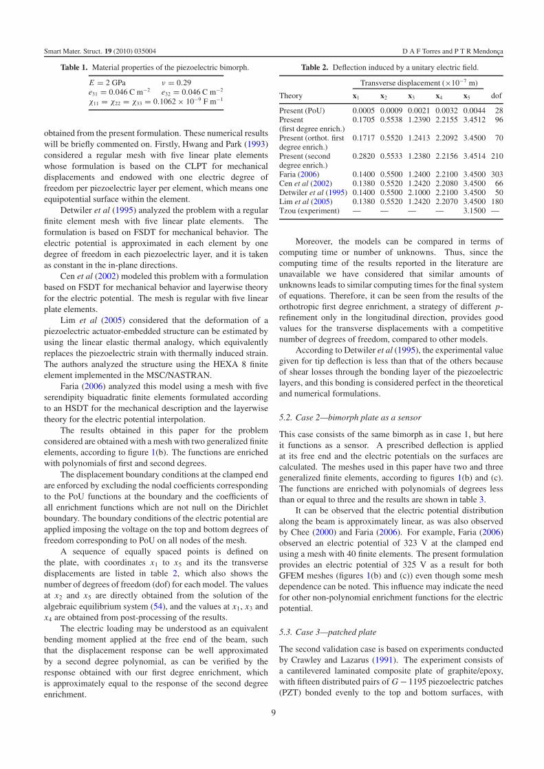
This problem consists of a bimorph working as an actuator.The top and bottom surfaces of the beam are subjected toelectric potentials of 0.5 V and −0.5 V, respectively, resultingin a unitary electric field across the thickness of the beam, andthe corresponding displacements are determined. This problemwas subjected to experimental measurements obtained by Tzouand Tseng (1990). Their experimental apparatus consists ofa cantilevered piezoelectric bimorph beam constructed of twolayers of PVDF bonded together and polarized in oppositedirections. The dimensions and discretized models used in thenumerical analysis reported here are shown in figure 1. Thematerial properties are given in table 1.
The experimental results obtained by Tzou and Tseng(1990) have been used to verify numerical results of severalresearchers, and some of these results are compared with those
8
Smart Mater. Struct. 19 (2010) 035004 D A F Torres and P T R Mendonca
Table 1. Material properties of the piezoelectric bimorph.
E = 2 GPa ν = 0.29e31 = 0.046 C m−2 e32 = 0.046 C m−2
χ11 = χ22 = χ33 = 0.1062 × 10⁻⁹ F m−1
obtained from the present formulation. These numerical resultswill be briefly commented on. Firstly, Hwang and Park (1993)considered a regular mesh with five linear plate elementswhose formulation is based on the CLPT for mechanicaldisplacements and endowed with one electric degree offreedom per piezoelectric layer per element, which means oneequipotential surface within the element.
Detwiler et al (1995) analyzed the problem with a regularfinite element mesh with five linear plate elements. Theformulation is based on FSDT for mechanical behavior. Theelectric potential is approximated in each element by onedegree of freedom in each piezoelectric layer, and it is takenas constant in the in-plane directions.
Cen et al (2002) modeled this problem with a formulationbased on FSDT for mechanical behavior and layerwise theoryfor the electric potential. The mesh is regular with five linearplate elements.
Lim et al (2005) considered that the deformation of apiezoelectric actuator-embedded structure can be estimated byusing the linear elastic thermal analogy, which equivalentlyreplaces the piezoelectric strain with thermally induced strain.The authors analyzed the structure using the HEXA 8 finiteelement implemented in the MSC/NASTRAN.
Faria (2006) analyzed this model using a mesh with fiveserendipity biquadratic finite elements formulated accordingto an HSDT for the mechanical description and the layerwisetheory for the electric potential interpolation.
The results obtained in this paper for the problemconsidered are obtained with a mesh with two generalized finiteelements, according to figure 1(b). The functions are enrichedwith polynomials of first and second degrees.
The displacement boundary conditions at the clamped endare enforced by excluding the nodal coefficients correspondingto the PoU functions at the boundary and the coefficients ofall enrichment functions which are not null on the Dirichletboundary. The boundary conditions of the electric potential areapplied imposing the voltage on the top and bottom degrees offreedom corresponding to PoU on all nodes of the mesh.
A sequence of equally spaced points is defined onthe plate, with coordinates x1 to x5 and its the transversedisplacements are listed in table 2, which also shows thenumber of degrees of freedom (dof) for each model. The valuesat x2 and x5 are directly obtained from the solution of thealgebraic equilibrium system (54), and the values at x1, x3 andx4 are obtained from post-processing of the results.
The electric loading may be understood as an equivalentbending moment applied at the free end of the beam, suchthat the displacement response can be well approximatedby a second degree polynomial, as can be verified by theresponse obtained with our first degree enrichment, whichis approximately equal to the response of the second degreeenrichment.
Table 2. Deflection induced by a unitary electric field.
Transverse displacement (×10−7 m)
Theory x1 x2 x3 x4 x5 dof
Present (PoU) 0.0005 0.0009 0.0021 0.0032 0.0044 28Present(first degree enrich.)
0.1705 0.5538 1.2390 2.2155 3.4512 96
Present (orthot. firstdegree enrich.)
0.1717 0.5520 1.2413 2.2092 3.4500 70
Present (seconddegree enrich.)
0.2820 0.5533 1.2380 2.2156 3.4514 210
Faria (2006) 0.1400 0.5500 1.2400 2.2100 3.4500 303Cen et al (2002) 0.1380 0.5520 1.2420 2.2080 3.4500 66Detwiler et al (1995) 0.1400 0.5500 2.1000 2.2100 3.4500 50Lim et al (2005) 0.1380 0.5520 1.2420 2.2070 3.4500 180Tzou (experiment) — — — — 3.1500 —
Moreover, the models can be compared in terms ofcomputing time or number of unknowns. Thus, since thecomputing time of the results reported in the literature areunavailable we have considered that similar amounts ofunknowns leads to similar computing times for the final systemof equations. Therefore, it can be seen from the results of theorthotropic first degree enrichment, a strategy of different p-refinement only in the longitudinal direction, provides goodvalues for the transverse displacements with a competitivenumber of degrees of freedom, compared to other models.
According to Detwiler et al (1995), the experimental valuegiven for tip deflection is less than that of the others becauseof shear losses through the bonding layer of the piezoelectriclayers, and this bonding is considered perfect in the theoreticaland numerical formulations.
5.2. Case 2—bimorph plate as a sensor
This case consists of the same bimorph as in case 1, but hereit functions as a sensor. A prescribed deflection is appliedat its free end and the electric potentials on the surfaces arecalculated. The meshes used in this paper have two and threegeneralized finite elements, according to figures 1(b) and (c).The functions are enriched with polynomials of degrees lessthan or equal to three and the results are shown in table 3.
It can be observed that the electric potential distributionalong the beam is approximately linear, as was also observedby Chee (2000) and Faria (2006). For example, Faria (2006)observed an electric potential of 323 V at the clamped endusing a mesh with 40 finite elements. The present formulationprovides an electric potential of 325 V as a result for bothGFEM meshes (figures 1(b) and (c)) even though some meshdependence can be noted. This influence may indicate the needfor other non-polynomial enrichment functions for the electricpotential.
5.3. Case 3—patched plate
The second validation case is based on experiments conductedby Crawley and Lazarus (1991). The experiment consists ofa cantilevered laminated composite plate of graphite/epoxy,with fifteen distributed pairs of G − 1195 piezoelectric patches(PZT) bonded evenly to the top and bottom surfaces, with
9

Smart Mater. Struct. 19 (2010) 035004 D A F Torres and P T R Mendonca
Figure 2. Cantilevered graphite/epoxy composite plate withdistributed piezoelectric sensors and actuators.
Table 3. Electric potential induced by a deflection at the end.
Electric potential (V)
Theory 0 x1 x2 x3 x4 x5
Present (PoU) mesh b 369 259 148 99 49 0Present (first degree enrich.)mesh b
245 211 176 160 144 128
Present (second degreeenrich.) mesh b
325 260 196 131 65 0
Present (third degree enrich.)mesh b
325 261 196 131 66 0
Present (PoU) mesh c 356 373 82 48 14 −21Present (first degree enrich.)mesh c
294 259 144 134 125 12
Present (second degreeenrich.) mesh c
327 262 196 131 65 0
Present (third degree enrich.)mesh c
325 262 196 131 65 0
Faria (2006) 280 255 195 130 70 45Detwiler et al (1995) 280 250 186 120 56 25Hwang and Park (1993) 287 245 175 120 60 30
thickness 0.25 mm (see figure 2). Two laminates were tested:the first one with the stacking sequence [0/45/−45]s, subjectedto electric potentials of 100 and 157.6 V and the second onewith the stacking sequence [30/30/0]s and subjected to anelectric potential of 188.8 V, both with total thickness 0.83 mm.
Detwiler et al (1995) modeled the problem with a FSDTisoparametric quadrilateral finite element with a formulationbased on an electric potential constant throughout the plane ofthe element.
Saravanos et al (1997) analyzed the problem using acompletely layerwise description in a bilinear finite elementformulation and considering a mesh with 16×9 finite elements.These authors used the following normalized form for thedeflections, consistent with the way the experimental resultswere published
T1 = w2
BT2 = 1
B
(w2 − (w1 + w3)
2
)
T3 = (w3 −w1)
B
(55)
Figure 3. Mesh used in the GFEM model of the cantileveredcomposite plate.
where w2, w1 and w3 are the transverse displacement alongthe midline and the two edges respectively, and B is the widthof the plate. These three normalized displacements represent,or approximate, the axial bending deflection, the transversebending curvature, and the twisting angle due to bending–twisting coupling, respectively. Furthermore, they considereda [0/45/−45]s lay-up cantilevered plate, whose deflection wasinduced applying a uniform electric field of 394 V mm−1, ofopposite polarity at the upper and lower piezoelectric patches.
Chee (2000), developed a formulation of piezoelectricplates considering HSDT and layerwise theory and imple-mented it using biquadratic serendipity finite elements. Theauthor presents the solution for the T1 displacement (55) froma model of this piezoelectric plate with a 12 × 7 finite elementmesh and applying an uniform electric potential of 100 V for a[0/45/−45]s lay-up and 120 V for a [30/30/0]s lay-up.
Lee (2001) also used biquadratic serendipity finiteelements formulated according to the layerwise theory, for bothmechanical and electrical behaviors, and showed numerical T1
results for this cantilevered composite plate modeled with a16 × 9 finite element mesh. Two situations were analyzed:application of (a) a uniform electric field of 394 V mm−1 fora [0/45/ − 45]s lay-up and (b) a uniform electric field of472 V mm−1 for a [30/30/0]s lay-up.
Faria (2006) also analyzed this problem using a mixedHSDT-LT formulation and considering a mesh with 12 × 7biquadratic serendipity finite elements for both [0/45/ − 45]s
and [30/30/0]s lay-ups subjected to uniform electric fields of100 V and 120 V, respectively. This author also presented onlythe results for T1 displacements.
The problem is solved with the present formulationconsidering the mesh shown in figure 3, using the PoUfunctions only, and isotropic enrichments of first and seconddegrees. The material properties are listed in table 4.
The displacement boundary conditions are applied in sucha way that just the PoU and the enrichment functions whichare not null on the Dirichlet boundary are eliminated. Hence,the contribution to the solution provided by the remainingenrichment functions is maintained on the clouds at thisboundary. This procedure is easily implemented since thecontours are straight lines and are parallel to the coordinateaxis. The electric boundary conditions are applied imposingthe voltage directly on the top and bottom electric degrees offreedom related to all elements with piezoelectric layers.
10

Smart Mater. Struct. 19 (2010) 035004 D A F Torres and P T R Mendonca
Figure 4. Longitudinal bending of a cantilevered [0/45/−45]s
composite plate subjected to 100 V.
Table 4. Material properties.
Properties Gr/epoxy PZT-4
Elastic properties
E1 (N mm−2) 142.86 × 10³ 62.97 × 10³
E2 (N mm−2) 9.70 × 10³ 62.97 × 10³
E3 (N mm−2) 9.70 × 10³ 62.97 × 10³
G12 (N mm−2) 6.00 × 10³ 24.20 × 10³
G23 (N mm−2) 4.00 × 10³ 24.20 × 10³
G13 (N mm−2) 6.00 × 10³ 24.20 × 10³
ν12 0.30 0.30ν23 0.37 0.30ν31 0.30 0.30
Piezoelectric coefficients
e15 (C mm−2) — 14.13 × 10⁻⁶
e14 (C mm−2) — 14.13 × 10⁻⁶
e31 (C mm−2) — 18.41 × 10⁻⁶
e32 (C mm−2) — 18.41 × 10⁻⁶
e33 (C mm−2) — 12.51 × 10⁻⁶
Dielectric permittivity
χ11 (F mm−1) — 15.30 × 10⁻¹⁰
χ22 (F mm−1) — 15.30 × 10⁻¹⁰
χ33 (F mm−1) — 15.00 × 10⁻¹⁰
Figure 4 shows the longitudinal bending (T1) of the[0/45/−45]s plate subjected to 100 V and figures 5 and 6 showthe transverse bending (T2) and twisting (T3), respectively,for the same lay-up and an electric potential of 157.6 V.Figures 7 and 8 also show the transverse bending and twisting,respectively, but for the [30/30/0]s plate, subjected to 188.8 V.
Figure 4 shows the convergence behavior of the solutionfor both first and second degree enrichments. The resultreported by Faria (2006) is not included in the figure becausethe curve would be too close to that of the present formulation.The differences in the results obtained for the deflection at theend of plate in the present study and in those of Saravanoset al (1997) and by Lee (2001) are due to the differences in themechanical kinematical hypothesis of each formulation. Thisis notable since the results for the present formulation and thoseof Chee (2000) differ only slightly, observing that the second
Figure 5. Transverse bending of a cantilevered [0/45/−45]s
composite plate subjected to 157.6 V.
Figure 6. Twisting of a cantilevered [0/45/−45]s composite platesubjected to 157.6 V.
Figure 7. Transverse bending of a cantilevered [30/30/0]s compositeplate subjected to 188.8 V.
polynomial degree provided by the serendipity finite elementsof Chee (2000) and the first degree enrichment of the presentare similar. Nevertheless, it should be pointed out that theGFEM formulation allows such a structure to be analyzed with
11

Smart Mater. Struct. 19 (2010) 035004 D A F Torres and P T R Mendonca
Figure 8. Twisting of a cantilevered [30/30/0]s composite plate subjected to 188.8 V.
the minimum amount of elements, according to the distributionof piezoelectric patches.
For the transverse bending, as shown in figures 5 and 7,the GFEM formulation shows good approximation capabilitiesas the enrichment degree increases. In addition, it isimportant to observe that the GFEM mesh requires the leastnumber of elements and nodes possible for this distribution ofpiezoelectric patches.
For the twisting results, as shown in figures 6 and 8, theGFEM formulation shows more flexibility to reproduce thedeformed shape compared to the results from the FSDT modelof Detwiler et al (1995) and exhibit convergence behavior forthe first and second degree enrichments.
6. Concluding remarks
The mixed layerwise-HSDT formulation for laminated plateswith piezoelectric layers represents an efficient tool formodeling adaptive plate structures. The third degreeexpansion of mechanical displacements with piecewise lineardiscretization of the electric potential is a reasonable kinematichypothesis for the phenomenon under analysis. Theverification of the respective implementation was conductedthrough comparison with the results of several cases reportedin the literature. The GFEM methodology for the enrichmentof subspaces built with a conventional finite element partitionof unity provides good approximation quality even when usinga fixed finite element mesh. As the enrichment processes isfrom the partition of unity, through adding especial functionsdefined on global coordinates, the enrichment degree may varyover the connected domain without loss of conformity. Thisalso leads to the possibility of enriching only some generalizedunknowns or modeling problems with singularities. Suchimprovement may be seen for approximation of either primalor dual unknowns, logically limited by the hypothesis adoptedfor the physical modeling. The formulation is complete inthe sense that it consistently considers the static as well asthe dynamic behavior of adaptive plates. The performance indynamic modeling will be the subject of a future publication.
Acknowledgments
D A F Torres gratefully acknowledges the financial supportprovided by the Brazilian government agency CAPES(Coordenacao de Aperfeicoamento de Pessoal de NıvelSuperior) during this research.
References
Allik H and Hughes T J R 1970 Finite element method forpiezoelectric vibration Int. J. Numer. Methods Eng. 2 151–8
Babuska I, Caloz G and Osborn J E 1994 Special finite elementmethods for a class of second order elliptic problems with roughcoefficients SIAM J. Numer. Anal. 31 945–81
Babuska I and Melenk J M 1997 The partition fo unity finite elementmethod Int. J. Numer. Methods Eng. 40 727–58
Barcellos C S, Mendonca P T R and Duarte C A 2009 A Ck
continuous generalized finite element formulation applied tolaminated Kirchhoff plate model Comput. Mech. 44 377–93
Barros F B, Barcellos C S and Duarte C A 2007 −p Adaptive Ck
generalized finite element method for arbitrary polygonalclouds Comput. Mech. 41 175–87
Cen S, Soh A-K, Long Y-Q and Yao Z-H 2002 A new 4-nodequadrilateral FE model with variable electrical degrees offreedom for the analysis of piezoelectric laminated compositeplates Compos. Struct. 58 583–99
Chee C Y K 2000 Static shape control of laminated composite platesmart structure using piezoelectric actuators PhD ThesisUniversity of Sydney
Chee C Y K, Tong L and Steven G P 1998 A review on the modelingof piezoelectric sensors and actuators incorporated in intelligentstructures J. Intell. Mater. Syst. Struct. 9 3–19
Cotoni V, Masson P and Cote F 2006 A finite element forpiezoelectric multilayered plates: combined higher-order andpiecewise linear C0 formulation J. Intell. Mater. Syst. Struct.17 155–66
Crawley E F and Lazarus K B 1991 Induced strain actuation ofisotropic and anisotropic plates AIAA J. 29 944–51
Detwiler D T, Shen M-H H and Vankayya V B 1995 Finite elementanalysis of laminated composite structures containingdistributed piezoelectric actuators and sensors Finite ElementsAnal. Des. 20 87–100
Duarte C A 1996 The hp-cloud method PhD Thesis The Universityof Texas at Austin
12

Smart Mater. Struct. 19 (2010) 035004 D A F Torres and P T R Mendonca
Duarte C A, Babuska I and Oden J T 2000 Generalized finite elementmethod for three-dimensional structural mechanics problemsComput. Struct. 77 215–32
Duarte C A, Hamzeh O N, Liszka T J and Tworzydlo W W 2001 Ageneralized finite element method for the simulation ofthree-dimensional crack propagation Comput. Methods Appl.Mech. Eng. 190 2227–62
Duarte C A, Kim D-J and Quaresma D M 2006 Arbitrarily smoothgeneralized finite element approximations Comput. MethodsAppl. Mech. Eng. 196 33–56
Duarte C A and Oden J T 1996 An h- p adaptive method using cloudComput. Methods Appl. Mech. Eng. 139 237–62
Faria A W 2006 Finite element modeling of composite platesincorporating piezoelectric sensors and actuators:implementation and numerical assesssment MSc DissertationFederal University of Uberlandia (abstract in English, text inPortuguese)
Gao J-X and Shen Y-P 2003 Active control of goemetricallynonlinear transient vibration of composite plates withpiezoelectric actuators J. Sound Vib. 264 911–28
Garcia O A 2003 Generalized finite elements in static analysis ofplates and shells PhD Thesis Federal University of SantaCatarina (abstract in English, text in Portuguese)
Garcia O A, Fancello E A and Mendonca P T R 2009 Developmentsin the application of the generalized finite element method tothick shell problems Comput. Mech. 44 669–82
Ha S K, Keilers C and Chang F K 1992 Finite element analysis ofcomposite structures containing distributed piezoceramicsensors and actuators AIAA J. 30 772–80
Hwang W S and Park H C 1993 Finite element modeling ofpiezoelectric sensors and actuators AIAA J. 31 930–7
Lage R G, Soares C M M, Soares C A M and Reddy J N 2004Layerwise partial mixed finite element analysis ofmagneto-electro-elastic plates Comput. Struct. 82 1293–301
Lee H-J 2001 Finite element analysis of active and sensorythermopiezoelectric composite materials Report 210892 GlennResearch Center—National Aeronautics and SpaceAdministration
Levinson M 1980 An accurate simple theory of the statics anddynamics of elastic plates Mech. Res. Commun. 7 343–50
Liew K M, He X Q, Tan M J and Lim H K 2004 Dynamic analysis oflaminated composite plates with piezoelectric sensor/actuatorpatches using the FSDT mesh-free method Int. J. Mech. Sci.46 311–31
Lim S M, Lee S, Park H C, Yoon K J and Goo N S 2005 Design anddemonstration of a biomimetic wing section using a lightweight
piezo-composite actuator (LIPCA) Smart Mater. Struct.14 496–503
Melenk J M 1995 On generalized finite element method PhD ThesisUniversity of Maryland
Melenk J M and Babuska I 1996 The partition of unity finite elementmethod: basic theory and application Comput. Methods Appl.Mech. Eng. 139 289–314
Oden J T, Duarte C A and Zienkiewicz O C 1998 A new cloud-basedhp finite element method Comput. Methods Appl. Mech. Eng.153 117–26
Oden J T and Reddy J N 1976 An Introduction to the MathematicalTheory of Finite Elements (New York: Wiley)
O’Hara P J 2007 Finite element analysis of three-dimensional heattransfer for problems involving sharp thermal gradients MScDissertation University of Illinois at Urbana-Champaign
O’Hara P J, Duarte C A and Eason T 2009 Generalized finite elementanalysis of three-dimensional heat transfer problems exhibitingsharp thermal gradients Comput. Methods Appl. Mech. Eng.198 1857–71
Reddy J N 1999 On laminated composite plates with integratedsensors and actuators Eng. Struct. 21 568–93
Reddy J N 2004 Mechanics of Laminated Composite Plates andShells: Theory and Analysis (Boca Raton, FL: CRC Press)
Saravanos D A 1997 Mixed laminate theory and finite element forsmart piezoelectric composite shell structures AIAA J.35 1327–33
Saravanos D A, Heyliger P R and Hopkins D A 1997 Layerwisemechanics and finite element for the dynamic analysis ofpiezoelectric composite plates Int. J. Solids Struct. 34 359–78
Strouboulis T, Babuska I and Copps K 2000 The design and analysisof the generalized finite element method Comput. MethodsAppl. Mech. Eng. 181 43–69
Strouboulis T, Copps k and Babuska I 2001 The generalized finiteelement method Comput. Methods Appl. Mech. Eng.190 4081–193
Strouboulis T, Zhang L and Babuska I 2003 Generalized finiteelement method using mesh-based handbooks: application toproblems in domains with many voids Comput. Methods Appl.Mech. Eng. 192 3109–61
Szabo B and Babuska I 1991 Finite Element Analysis (New York:Wiley)
Tzou H S and Tseng C I 1990 Distributed piezoelectricsensor/actuator design for dynamic measurement/control ofdistributed parameter systems: a piezoelectric finite elementapproach J. Sound Vib. 138 17–34
13