analysis of nonlinear di usion equations of second and
TRANSCRIPT

Analysis of nonlineardiffusion equations of
second and fourth order
Dissertationzur Erlangung des Grades
Doktorder Naturwissenschaften
am Fachbereich Physik, Mathematik und Informatikder Johannes Gutenberg-Universitat
in Mainz
Maria Pia Gualdanigeboren in Montevarchi (Italien)
Mainz, Juli 2005

Abstract
Due to the ongoing miniaturization of semiconductor devices, quantumeffects play a more and more dominant role. Usually, quantum phenomenaare modeled by using kinetic equations, but sometimes a fluid-dynamicaldescription presents several advantages; for example the better tractabilityfrom a numerical point of view and the assignation of boundary conditions.In the following work we study three fluid-type nonlinear partial differentialequations of the second and fourth order; these models are related to themodeling of semiconductor devices. The first part concerns the study of afully implicit semidiscretization in time and of the long-time asymptotics ofa Fokker-Planck equation of degenerate type. The second part is devoted tothe study of a quantum hydrodynamic model in one space dimension andthe asymptotic decay of the model is formally shown. In the last sectionof the work existence and long-time behaviour of a nonlinear fourth-orderparabolic equation (reduced quantum drift-diffusion model) in one spacedimension are proved and some numerical examples are given.
2
Contents
Chapter 1. Introductory Overview 4
1.1 Short summary of part I . . . . . . . . . . . . . . . . . . . . . 10
1.2 Short summary of part II . . . . . . . . . . . . . . . . . . . . . 12
1.3 Short summary of part III . . . . . . . . . . . . . . . . . . . . 15
Chapter 2. Semidiscretization and long-time asymptotics 20
2.1 Semidiscretization of a nonlinear diffusion equation and nu-merical examples . . . . . . . . . . . . . . . . . . . . . . . . . 20
2.2 Evolution of the 1-D Wasserstein distances . . . . . . . . . . . 37
Chapter 3. Analysis of the viscous quantum hydrodynamicequations 43
3.1 Existence of solutions . . . . . . . . . . . . . . . . . . . . . . . 47
3.2 Uniqueness of solution . . . . . . . . . . . . . . . . . . . . . . 50
3.3 Asymptotic limits . . . . . . . . . . . . . . . . . . . . . . . . . 54
3.4 Exponential decay in time . . . . . . . . . . . . . . . . . . . . 56
Chapter 4. A nonlinear fourth-order parabolic equation 61
4.1 Existence and uniqueness of stationary solution . . . . . . . . 62
4.2 Existence of transient solutions . . . . . . . . . . . . . . . . . 66
4.3 Long-time behavior of the solutions . . . . . . . . . . . . . . . 72
4.4 Numerical examples . . . . . . . . . . . . . . . . . . . . . . . . 76
Bibliography 80
3

Chapter 1
Introductory Overview
In the following we shall deal with the study of several nonlinear partialdifferential equations of second and fourth order, describing differentdiffusion phenomena and related to the modeling of semiconductor devices.In this sense it is possible to divide this work into three independent parts:
I. The study of a Fokker-Planck equation.II. The investigation of stationary solutions to a quantum
hydrodynamic model.III. The study of a reduced quantum drift-diffusion model.
The modern computer and telecommunication industry relies heavily on theuse of semiconductors devices. The reason of the rapid development andsuccess in the semiconductor technology is refereed to the ongoing devicesminiaturization. The microelectronics industry produces very miniaturizedcomponents with small characteristic length scale, like tunneling diodes,which have a structure of only few nanometer length. In such compo-nents quantum phenomena become no more negligible, even sometimespredominant and the physical phenomena have to be described by quantummechanics equations.A semiconductor device needs an input (generally light or electronic signal)and produces an output (light or electronic signal); the device is connectedto the electric circuit by contacts at which a voltage is applied. We areinteresting in devices which produce electric signals, for example currentof electrons generated by the applied potential. In this case the relationbetween the input (applied voltage) and the output (current throughone contact) is a curve (not necessary a function) called current-voltagecharacteristic.Depending on the devices structure, the transport of particles can be verydifferent, due to several physical phenomena, like drift, diffusion, scattering
4

Chapter 1. Introductory Overview 5
and quantum effects. The more appropriate way to describe a large numberof particles flowing through a device is a kinetic or a fluid-dynamic typedescription. On the other hand, electrons are in a semiconductor crystalquantum objects, for which a wave-like description using the Schrodingerequation seems to be necessary. Therefore there are several mathematicalmodels, which are able to describe particular phenomena in particulardevices. These models vary for complexity and for mathematical propertiesand build a hierarchy, in which three classes can be distinguishes: kineticmodels, fluid-dynamical models and quantum models.
In a quantum dynamical view, each single electron is interpreted as awave; the motion of an electron ensemble of M particles in a vacuum underthe influence of a (real-valued) electrostatic potential V is described by thewave function ψ(x, t), solution to the Schrodinger equation
iε∂ψ
∂t= −ε
2
2
M∑
j=1
∆xjψ − V (x, t)ψ, x ∈ R
dM , t > 0.(1.0.1)
The letter i denotes the complex unit and ε the scaled Planck constant.Another equivalent formulation to the Schrodinger description of the motionof an electron ensemble is given by the kinetic (Wigner) formulation. Letψ(x, t) be a solution to (1.0.1); we define the density matrix
ρ(r, s, t) := ψ(r, t)ψ(s, t), r, s ∈ RdM , t > 0.
The Wigner function has been introduced by Wigner (1932), defined as
w(x, k, t) :=1
(2π)dM
∫
RdM
ρ(x +ε
2η, x− ε
2η, t)eiη·kdη,
and formally solves the following equation
∂w
∂t+ k · ∇xw − Θ[V ]w = 0, x, k ∈ R
dM , t > 0,(1.0.2)
where (x, k) are the position-momentum variables; Θ[V ] is a pseudo-differential operator [71], defined as
(θ[V ])(w)(x, k, t) =1
(2π)dM
∫
RdM
∫
RdM
i
ε
[
V(
x +ε
2η, t
)
− V(
x− ε
2η, t
)]
× w(x, k′, t)ei(k−k′)·ηdk′ dη,
applied to the electrostatic potential V , which is usually self-consistent andgiven by the Poisson equation
−λ2∆V = n− C(x),(1.0.3)
Chapter 1. Introductory Overview 6
where λ is the semiconductor permittivity, C(x) a positive function describingthe concentration of the fixed charge background ions in the semiconductorcrystal and n the particle density, defined as n(x, t) :=
∫
Rd w(x, k, t) dk.In the mathematical modeling for semiconductor devices it is necessary totake into account also the physical effects coming from short-range parti-cle interactions, like collisions of electrons with other electrons or with thecrystal lattice. In particular, in semiconductor crystals there are three mainscattering phenomena: electron-phonon scattering, ionized impurity scatter-ing and carrier-carrier scattering. Collision effects can be described at thekinetic level by the Wigner-Fokker-Planck equation
∂w
∂t+ k · ∇xw − Θ[V ]w = Q(w), (x, k) ∈ R
2d, t > 0.(1.0.4)
The term Q(w) is called collision operator ; it models the interaction of theelectrons with the phonons of the crystal lattice (oscillators) and has theform
Q(w) = α∆kw +1
τdivk(kw) + βdivx(∇kw) + ν∆xw,(1.0.5)
with α, β, τ and ν positive constants. The model (1.0.4), (1.0.5) governs thedynamical evolution of an electron ensemble in the single-particle Hartreeapproximation interacting dissipatively with an idealized heat bath consist-ing of an ensemble of harmonic oscillators and modeling the semiconductorlattice. Problem (1.0.4), (1.0.5) has been derived in [20, 35] and studied in[7, 8, 9].Due to the nonlinearities and to the high number of independent variables,the mathematical analysis of kinetic models can be very complicated. Simplermacroscopic models have been derived from (1.0.4); these models describethe evolution of macroscopic quantities, like electron and hole density. Oneof the advantages of a fluid-dynamical description concerns numerical sim-ulations, which require in this case less computation power. Moreover, assemiconductor devices are modeled in a bounded domain, it is easier to findphysically relevant boundary conditions for macroscopic variables then forwave or for the Wigner function, for which the natural physical setting isbased on an unbounded domain.The particle density n(x, t) and the current density J(x, t) are defined re-spectively as the zeroth and first moment of the Wigner function
n(x, t) :=
∫
Rd
w(x, k, t) dk, J(x, t) :=
∫
Rd
kw(x, k, t) dk,
and macroscopic equations are derived from (1.0.4) using the momentmethod. We multiply (1.0.4) by 1 and k and after integration over k ∈ R
d,
Chapter 1. Introductory Overview 7
we get the so-called moment equations
∂〈w〉∂t
+ div〈kw〉 = ν∆〈w〉,(1.0.6)
∂〈kw〉∂t
+ div〈k ⊗ kw〉 − 〈w〉∇V = −〈kw〉τ
− βdiv〈w〉 + ν∆〈kw〉,
where 〈g(k)〉 :=∫
Rd g(k) dk. The goal of this method is to express each termof the above system of equations in term of the moments 〈w〉 and 〈kw〉. Themain difficulties arise now from the flux 〈k⊗kw〉 , which cannot be rewrittenwith help of the first and second order moment. Therefore a closure conditionis needed. As in the case of the classical kinetic theory, we achieve the closurecondition by assuming as in [40] that the Wigner function w is close to awave function displaces equilibrium density such that
w(x, k, t) = weq(x, k − u(x, t), t),
where u(x, t) is some group velocity,
weq = A(x, t)exp(
− |k|22T
+V
T
)[
1 + ε2( 1
8T 2∆xV(1.0.7)
+1
24T 3|∇xV |2 −
1
24T 3
d∑
i,j=1
kikj∂2V
∂xi∂xj
)
+O(ε4)]
,
and T is the electron temperature. The function (1.0.7) is derived from anO(ε4) approximation of the thermal equilibrium density first given by Wigner[79]. The function A(x, t) is assumed to be slowly varying in x and t. Thenthe first moments are 〈w〉 = n and 〈kw〉 = J and
〈k ⊗ kw〉 =J ⊗ J
n+ nT Id − ε2
12Tn(∇⊗∇)V +O(ε4).(1.0.8)
The formula (1.0.7) implies that n equals eV/T times a constant, up to theterm of order O(ε2), and therefore, if the temperature is slowly varying,
∂2 logn
∂xi∂xj=
1
T
∂2V
∂xi∂xj+O(ε2).
Using this condition we can replace all second derivatives of V by secondderivatives of logn, making an error of order O(ε4). This yields to the viscousquantum hydrodynamic equations
∂n
∂t+ divJ = ν∆n, x ∈ R
d, t > 0,(1.0.9)
∂J
∂t+ div
(
J ⊗ J
n
)
+ ∇(nT ) + n∇V − ε2
2n∇
(
∆√n√n
)
= −Jτ
+ ν∆J,

Chapter 1. Introductory Overview 8
where the electrostatic potential V is self-consistent and given by (1.0.3).The above system consists in conservation laws for the particle and for
the current density. The quantum term ε2
2n
(
∆√
n√n
)
can be interpreted
as a quantum self-potential term with the Bohm potential ∆√
n√n
or as the
divergence of the pressure tensor P = ε2
4n(∇ ⊗ ∇) logn. The terms J
τ,
ν∆n and ν∆J model interactions of the electrons with the phonons of thesemiconductor crystal lattice. The term nT describes the pressure tensor.In the literature we can find several assumptions for the temperature T ; thefunction T can be assumed to be constant, a function of the particle densityT (n), as in the fluid-dynamical case, or described by an additional equation.In this last case, the additional equation can be derived from the Wignerequation (1.0.4) by a moment method, similar as above, multiplying (1.0.4)by the second moment 1
2|k|2 and integrating oder k ∈ R
d. In the followingwe consider the temperature as a function of the particle density T = T (n).Setting ν = 0 in (1.0.9) we get the so-called inviscid quantum hydrodynamicmodel .
We perform now in the inviscid quantum hydrodynamic model thefollowing diffusion scaling: in (1.0.9) with ν = 0 we substitute t by t/τ andJ by Jτ , where τ is the relaxation time constant. After scaling we obtain
τ∂n
∂t+ τdivJ = 0, x ∈ R
d, t > 0,(1.0.10)
τ 2∂J
∂t+ τ 2div
(
J ⊗ J
n
)
+ ∇(nT (n)) + n∇V − ε2
2n∇
(
∆√n√n
)
= −J.
If the constant τ is small, then the above system describes a situation forlarge time-scale and small current density. Computing formally the limitτ → 0 in (1.0.10), the quantum drift-diffusion model is derived
∂n
∂t+ divJ = 0,(1.0.11)
J = −∇(nT (n)) − n∇V +ε2
2n∇
(
∆√n√n
)
.
The model consists in nonlinear continuity equation for the particle density;the current density J is given by the sum of the diffusion current ∇nT (n)and of the drift current nE, where E is the sum of the electrostatic potential
field with a quantum term, E = ∇(
V − ε2
2∆√
n√n
)
.
For vanishing scaled Planck constant ε = 0 we obtain the classical drift-diffusion model
∂n
∂t+ divJ = 0, J0 = −∇(nT (n)) − n∇V.(1.0.12)
Chapter 1. Introductory Overview 9
Recently another derivation of the quantum drift-diffusion model has beenpresented [32]; the model is derived from the Wigner equation (1.0.4) with aBGK-collision operator via a moment method and using as closure conditionthe entropy minimization principle. Let
Q(w) := M [w] − w
be the collision operator, where τ is the relaxation time and M [w] the quan-tum Maxwellian. The function M [w] is defined as a minimizer of a quantumentropy, subject to the constraint of a given particle density. More precisely,we introduce the free energy functional
H(w) =
∫
Rd
∫
Rd
w
(
Ln w − 1 +|k|22
− V (x)
)
dx dk
(2πεd).
The ”quantum logarithm” operator Ln is defined as Ln(w) =W (logW−1(w)), where W is the Wigner transform and W−1 the inverse(also called Weyl’s quantization) defined as
(W−1[w])φ(x) =
∫
R2d
w
(
x + y
2, k, t
)
φ(y)eik(x−y) dkdy
(2πεd),
for suitable φ(x). The quantum Maxwellian M [w] is assumed to be the min-imizer of H(w) under the constraint of given particle density, more precisely
H(M [w]) = min
H(w) |∫
Rd
w(x, k) dk = n(x), ∀x ∈ Rd
.
The quantum drift diffusion equations come now from a diffusion limit; werescale (1.0.4) in time, replacing t by t/δ and Q(w) by Q(w)/δ. This yields
δ∂wδ
∂t+ k · ∇xwδ − Θ[V ]wδ =
1
δ(M [wδ] − wδ), (x, k) ∈ R
2d, t > 0.
It can be proved that wδ → w0 as δ → 0 and the functions n :=∫
Rd w0 dkand P :=
∫
Rd k ⊗ k w0 dk satisfy the equations
∂n
∂t+ divJ = 0, J = divP − n∇V.(1.0.13)
Taking now an approximation of the function w0 (Chapman-Enskog method),which yields
J = J0 +O(ε4),
equations (1.0.13) can be rewritten as
∂n
∂t+ divJ = 0, J0 = −∇n− n∇V +
ε2
6n∇
(
∆√n√n
)
,
with constant temperature T = 1. Note that the Bohm potential in theabove equation has been derived by a factor 3 compared to the expression in(1.0.11). The physical explanation of this discrepancy has not been found.

Chapter 1. Introductory Overview 10
1.1 Short summary of part I
The first part of the work concerns the analysis of a fully implicit semidis-cretization in time and the long-time behaviour of equations of the form
∂n
∂t+ divJ = 0, x ∈ Ω ⊂ R
d, t > 0,(1.1.1)
where the current density J is given by
J = −∇f(n) − n∇V,(1.1.2)
with n the electron density and V the electrostatic potential. The functionf(n) describes the particle pressure and it is given by f(n) = n T (n), withT (n) the temperature. If f ′(0) = 0, the diffusion term in parabolic equationslike (1.1.1), (1.1.2) becomes of degenerate type.The family of equations (1.1.1), (1.1.2) include drift-diffusion type models(1.0.12), where the potential is given by the Poisson equation, nonlinearFokker-Planck equations, where V (x) is assumed to be confined and generalnonlinear diffusion equations, where V (x) ≡ 0.The existence analysis of (1.1.1), (1.1.2) with a confining potential or incase V ≡ 0 is done in [25, 75]. The fine description of long-time asymp-totics for nonlinear diffusion equations like (1.1.1), (1.1.2) has attracted inthe last years many mathematicians; the interest on this problem is basedon a bring-up of new ideas coming from different communities: the entropyapproach from kinetic theory, having its roots in the famous H-Theorem forthe Boltzmann equation [27, 65], the optimal mass transport theory, givinga geometric point of view of these equations [66, 26, 2, 3] and variationaltechniques related to new Gagliardo-Nirenberg inequalities [36].Nonlinear diffusion equations without confinement, V (x) ≡ 0, are expectedto diffuse as t → ∞, and thus, solutions vanish as t → ∞ with an expan-sion of their support or their tails depending whether the diffusion is slowor fast. On the contrary, nonlinear Fokker-Planck equations are expectedto stabilize towards a steady state n∞, defined by setting the flux to zero∇V + ∇h(n∞) = 0, where h(n) :=
∫ n
1f ′(s)
sds. A rigorous proof of this
stabilization was done in [25] in L1 by using an entropy-entropy productionapproach. The stationary state was characterized as the unique minimizerin the space of integrable functions with given mass of a suitable functionalthat we call entropy. This entropy functional was then proved to be a Lya-punov functional for the equation and thus, the study of its evolution gavethe desired convergence rate. We refer to [27, 25, 65] for details. More-over, generalized Log-Sobolev inequalities were obtained in [25] relating theentropy to the entropy production.
Chapter 1. Introductory Overview 11
Equations like (1.1.1), (1.1.2), either with V ≡ 0 or V 6= 0, share remarkableproperties with respect to Wasserstein distances for probability measures.This remarkable property of the family of equations (1.1.1), (1.1.2) is thatassuming that V (x) is convex, their flow map is a global contraction for the2-Wasserstein distance [66, 26, 2, 3]. Moreover, in the one dimensionalcase equations (1.1.1), (1.1.2) under the convexity assumption on V (x), arecontractions for all Wasserstein distances [28, 23].Nonlinear Fokker-Planck equations with confining potential V (x) = 1
2|x|2
and nonlinearity f(n) = nm are equivalent through an explicit change ofvariables to the nonlinear diffusion equation with V (x) ≡ 0 and f(n) = nm
and therefore, the study of their long-time behaviour is equivalent too. Infact, the stabilization towards equilibrium of the nonlinear Fokker-Planckequation translates into a self-similar behavior as t → ∞ for the nonlineardiffusion equation, in the sense that all solutions resemble a self-similarprofile as t → ∞. This self-similar profile is the well-known Barenblattprofile for homogenous nonlinear diffusions.
In Chapter 2 we analyze the semidiscretization based on the implicitEuler scheme of nonlinear Fokker-Planck equation (1.1.1), (1.1.2) withconfining potential in a bounded domain.In [10] the large time behaviour for an implicit semidiscretization intime of (1.1.1), (1.1.2) in the whole space with f(n) = n and confiningpotential is studied. We shall recall that the analytical methods used in[10] for the linear case are not helpful if f(n) is of degenerate type; sincethe staedy-state in the linear case f(n) = n is strictly positive, given byn∞ := e−V , weighted Sobolev spaces like L2(n−1
∞ ), equipped with the innerproduct 〈n1, n2〉n−1
∞
:=∫
Rdn1n2
n∞
dx, can be defined and some property likeconservation of mass can be easily proved. But the most important differencebetween the linear and the degenerate case consists on the treatment ofthe convection term n∇V ; since, if f(n) = n, the staedy-state is given byn∞ = e−V , the current density J = ∇f(n) + n∇V can be rewritten as
J = n∞∇(
nn∞
)
, which simplifies the analysis considerable.
The implicit Euler scheme for (1.1.1), (1.1.2) in case of degenerate diffusionterm in the whole space has not yet been investigated.We will show moreover that the semidiscretization of (1.1.1), (1.1.2)preserves the non-increasing behaviour of the entropy functional.In section 2.2 we deal with the long-time behaviour of (1.1.1), (1.1.2) incase V ≡ 0 and f(n) = nm. More precisely, the contractivity of Wassersteindistances in one space dimension is used to obtain a bound on the expansionrate of the support of solutions. It is well known that the degeneracy at leveln = 0 of the diffusivity D(n) = mnm−1 causes the phenomena called finitespeed of propagation. This means that the support of the solution n(·, t)
Chapter 1. Introductory Overview 12
to (1.1.1), (1.1.2) is a bounded set for all t ≥ 0. In fact it can be provedthat the solution n(x, t) as t → +∞ converges to the Barenblatt functionwith the same mass as the initial data. This result is already known sincethe work of J.L. Vazquez [74], but here we will give a alternative and verysimple proof of the finite propagation property, by using mass transportationtechniques.Although several qualitative properties of the solutions for general nonlineardiffusion equations have been obtained [57], there is no result concerningasymptotic profiles of general diffusion equations except in the case ofpower-like behavior for small values of n.
1.2 Short summary of part II
In this part of the work we investigate the one-dimensional stationary solutionof the viscous quantum hydrodynamic model
nt + Jx = νnxx,(1.2.1)
Jt +
(
J2
n
)
x
+ Tnx − nVx − ε2
2n
(√nxx√n
)
x
= −J
τ+ νJxx,
λ2Vxx = n − C(x) x ∈ (0, 1), t > 0,
with boundary conditions
n(0) = n(1) = 1, nx(0) = nx(1) = 0, V (0) = V0, J(0) = J0,
where n(x, t) describes the electron density, J(x, t) the current density andV (x, t) the electrostatic potential. The function C(x) describes the concen-tration of fixed background charges. The physical constants are the (scaled)Planck constant ε, the Debye length λ, the (scaled) temperature T supposedto be constant, the positive constant ν called viscosity and the (scaled) mo-mentum relaxation time τ . This model can be derived by a moment method[40], similarly as in the case of the quantum hydrodynamic model, from aWigner-Fokker-Planck equation (1.0.4) with a collision operator of the form(1.0.5).Concerning the mathematical analysis of the stationary inviscid quantumhydrodynamic model ((1.2.1) with ν = 0), many results are available[44, 49, 39, 81]. It has been shown (in one and several space dimensions)that there exists a weak solution to (1.2.1) with ν = 0 (and for various choicesof the boundary conditions), if a subsonic-type condition of the form
(1.2.2)J0
n<
√
T +ε2
4in (0, 1),
Chapter 1. Introductory Overview 13
is satisfied, i.e., if the current density is small enough. (Recall that an Eulerflow is called subsonic if J0/n <
√T .) Moreover, for special boundary con-
ditions, it has been proved [39] that the quantum hydrodynamic equationsdo not possess a weak solution if the current density is sufficiently large.The main difficulty in the existence analysis (besides of the mathematicaltreatment of the third-order quantum term) is the convection term (J 2/n)x.In fact (see [39]) this term may force the particle density to cavitate if thecurrent density is large enough. Without this term, the stationary equations(still with ν = 0) become the quantum drift-diffusion model for which a so-lution exists for any data [15]. The third-order quantum term possesses aregularizing effect since the condition (1.2.2) allows for slightly “supersonic”flows [44].
The question arises if, as in the case of the classical hydrodynamic equations,the viscous terms ν∆n and ν∆J regularize the equations in such a way thatthe existence of solutions can be proved for all values of the current densities.In this work we give a partial answer to this question.
More precisely, we prove the existence of classical solutions if the following“weakly supersonic” condition holds:
(1.2.3)J0
n<
1√2
√
T +ε2
16+ν
τin (0, 1).
Thus, the current density is allowed to be large if either the viscosity ν islarge or the (scaled) relaxation time is small enough. The reason for thisrestriction comes from the fact that, roughly speaking, the viscous term νJxx
can be reformulated (up to a factor) as the third-order quantum term. Infact, integrating Jx = νnxx and using the boundary condition for J we obtainJ = νnx + J0, which gives
(
J2
n
)
x
− νJxx = −2ν2n
(
(√n)xx√n
)
x
+
(
J20
n
)
x
+ 2νJ0(log n)xx,
and therefore, we can reformulate equation (1.2.1) formally as
(
J20
n
)
x
+(
T +ν
τ
)
nx − nVx −(
2ν2 +ε2
2
)
n
(
(√n)xx√n
)
x
= −J0
τ− 2J0ν(log n)xx.(1.2.4)
This formulation shows that the viscous terms indeed regularize the equations(as the coefficient of the quantum term becomes larger) but there is still aconvection term which may force the solutions to cavitate for large values ofthe current density J0. (Unfortunately, the method in [39] cannot be appliedto prove this conjecture rigorously.) Thus we expect a similar restriction

Chapter 1. Introductory Overview 14
on the current density as (1.2.2), but allowing for larger current densities.However, for sufficiently large ν/τ , we can allow for “supersonic” currentdensities J0/n >
√
T + ε2/4. We also remark that the above argument onlyholds in one space dimension. For the multi-dimensional problem, no resultsare available. This situation is similar to the inviscid quantum hydrodynamicequations, where mathematical results are essentially only available in onespace dimension (except [49]).
In order to prove the existence of solutions to (1.2.4), we rewrite (1.2.4) as afourth-order equation and employ the technique of exponential transforma-tion of variables n = eu as in [44] (first used in [18]). The existence of a weaksolution u ∈ H2(0, 1) provides a weak solution n = eu which is strictly posi-tive. Notice that maximum principle arguments can generally be not appliedto third- or fourth-order equations, and therefore, the exponential transfor-mation of variables circumvents this fact to prove positive lower bounds forthe particle density. As a second result we prove the uniqueness of stationarysolutions of (1.2.1) in one space dimension for sufficiently small parametersν, ε and J0. In semiconductor problems it is well known that uniqueness ofsolutions can only be expected for sufficiently small current densities sincethere are devices based on multiple solutions.
Using u = logn as a test function in the weak formulation of the fourth-orderequation, we obtain the estimate
(1.2.5)
(
ν2 +ε2
4
)
‖uxx‖L2 +
(
T +ν
τ
)
‖ux‖L2 ≤ K,
where K > 0 is a constant not depending on u, ν or ε (see Lemma 3.6). Thisinequality is the key estimate of chapter 3. It provides an H1 bound for uindependently of ν and ε. This allows to perform the inviscid limit ν → 0and the semiclassical limit ε→ 0. These limits as well as the combined limitν2 + ε2 → 0 are shown in Section 3.3.
A numerical study of the viscous quantum hydrodynamic model, includingthe asymptotic behavior of the solutions for small parameters (ν and ε), ispublished in [55, 52].
In Section 3.4 the long-time asymptotics of solutions to (1.2.1) in one spacedimension towards the so-called thermal equilibrium state (no current flow)is studied. Special thermal equilibrium functions are given by n = 1, J = 0and V = 0 in Ω = (0, 1) and we prove that any strong solution of (1.2.1)with initial data n(·, t) = nI and J(·, t) = JI and boundary conditions
n = 1 nx = 0 V = 0, on ∂Ω × (0,∞)∫
∂Ω
J
[
Jx
(
ε2
4ν+ ν
)
− 1
2J2
]
(·, t)ds = 0 t > 0
Chapter 1. Introductory Overview 15
converges exponentially fast to the unique thermal equilibrium state(n, J, V ) = (1, 0, 0).For the proof we assume, but we have not proved yet, that the system(1.2.1) has a global in time solution. The result of global in time existencepresents several difficulties; the main one concerns the effective current den-sity J−νnx, which is not constant anymore, contrary to the stationary case.Therefore the idea to rewrite the system as one equation for the particle den-sity is not useful. We can expect to get local-in-time existence of solutions, or”small” solutions globally in time, starting with initial data near the thermalequilibrium; these results can be proved by a Galarkin method, which yieldsexistence of solutions by standard ODE methods. The main question arisesnow if the particle density becomes zero at a certain time and if the linearphysical viscosity terms ν∆n and ν∆J are enough to prevent the function nto cavitate. No results are available in the literature.The proof of the exponential decay to the thermal equilibrium is based onthe entropy/entropy dissipation method, which is applied here for the firsttime to a third-order equation. Let
E(t) :=
∫ 1
0
[
ε2
2(√n)2
x + T (n(logn− 1) + 1) +λ2
2V 2
x +1
2
J2
n
]
(x, t)dx ≥ 0,
be the free energy functional, consisting on quantum energy, thermodynam-ical entropy, electric energy and kinetic energy of the system; the idea is toderive an inequality of the form
E(t) +
∫ t
0
∫ 1
0
P (x, t)dxds ≤ E(0),
where the entropy dissipation rate P (x, t) depends on the variables and hisderivatives. We show that:
∫ 1
0
P (x, t)dx ≥ γE(t)
for some γ > 0 and thus Gronwall’s lemma implies:
E(t) ≤ E(0)e−γt, t ≥ 0.
Finally Poincare inequality gives convergence rate of (n, J, V ) to the thermalequilibrium.
1.3 Short summary of part III
The third part of this work concerns the analysis of a simplified transientquantum drift diffusion model (1.0.11).

Chapter 1. Introductory Overview 16
The mathematical analysis and the numerical understanding of (1.0.11) inthe stationary case is now in a rather advanced state. The stationary problemhas been solved in [15], thermal equilibrium problem in [72] and a generalizedGummel iteration for an efficient numerical treatment in the one dimensionalspace has been developed in [68].Concerning the transient case, only partial results are known. The crucialproblem in the analysis comes from the fourth-order nature of the system. Inorder to understand better the influence of the fourth order term, we studieda simplified model: setting vanishing temperature and zero electric field in(1.0.11), the system can be rewritten as a fourth-order parabolic equationfor the particle density. In one space dimension, assuming smooth nonvacumsolutions, the Bohm potential differential operator (n ((
√n)xx/
√n)x)x can be
equivalently rewritten as (n(log n)xx)xx and system (1.0.11) reduces to thenonlinear fourth order parabolic problem
∂tn+ (n(log n)xx)xx = 0, n(·, 0) = nI(·).(1.3.1)
Equation (1.3.1) also arises as a scaling limit in the study of interface fluc-tuations in a certain spin system [34]. In quantum semiconductor modeling,Dirichlet-Neumann boundary conditions of the type
(1.3.2) n(0, t) = n(1, t) = 1, nx(0, t) = nx(1, t) = 0, t > 0,
have been employed to model resonant tunneling diodes in Ω = (0, 1) [53].The existence of global weak solutions to (1.3.1)-(1.3.2) has been proved in[54].The boundary conditions (1.3.2) simplify the analysis of (1.3.1) considerably.Indeed, one of the main ideas of the existence proof is to employ an exponen-tial transformation of variables, n = ey. In the new variable y, the boundaryconditions are homogeneous. Thus, using, for instance, the test function yin the weak formulation of (1.3.1), no integrals with boundary data appear.
The boundary conditions (1.3.2) follow from physical considerations like thecharge neutrality at the boundary contacts, i.e. n−C = 0 at x = 0, 1, whereC = C(x) models fixed background charges. Numerical results show that theNeumann boundary conditions for the density n should be non-homogeneousfor ultra-small semiconductor devices (see Section 4 in [67]). Moreover, whenthe values of the doping profile C(x) are different at the contacts, the Dirich-let boundary conditions satisfy n(0, t) 6= n(1, t). Therefore, we wish to studythe more general non-homogeneous boundary conditions(1.3.3)
n(0, t) = n0, n(1, t) = n1, nx(0, t) = w0, nx(1, t) = w1, t > 0,
where n0, n1 > 0 and w0, w1 ∈ R. The treatment of this non-homogeneitiesis also interesting from a mathematical point of view. Indeed, almost all
Chapter 1. Introductory Overview 17
results for (1.3.1) (and for related fourth-order equations like the thin-filmmodel [16]) are shown only for periodic or no-flux boundary conditions orfor whole-space problems, in order to avoid integrals with boundary dataand to use conservation of mass property
∫
Ωn(x, t) dx =
∫
ΩnI(x) dx for all
t > 0. In this work, we show how to deal with non-homogeneous boundaryconditions for equation (1.3.1).
More precisely, we show (i) the existence and uniqueness of a classical pos-itive solution n∞ to the stationary problem corresponding to (1.3.1), (ii)the existence of global nonnegative weak solutions n(·, t) to the transientproblem (1.3.1), (1.3.3), and (iii) the exponential convergence of n(·, t) toits steady state n∞ as t → ∞ in the L1 norm, under the assumption thatthe boundary data is such that log n∞ is concave. The long-time behavioris illustrated by numerical experiments. Notice that this is the first result ofthe stationary problem corresponding to (1.3.1) in the literature (if (1.3.2)or periodic boundary conditions are assumed, the steady state is constant).We also remark that the Wasserstein techniques of [41] cannot be applied to(1.3.1), (1.3.3) since this technique relies on the conservation of the L1 normwhich is not the case here. The long-time behavior of solutions to (1.3.1) hasbeen studied for periodic boundary conditions [19, 37] and for the boundaryconditions (1.3.2) [56]. In particular, it could be shown that the solutionsconverge exponentially fast to its (constant) steady state. The decay ratehas been numerically computed in [24]. No results are available up to nowfor the case of the non-homogenous boundary conditions (1.3.3).The first main result is the existence and uniqueness of stationary solutionsneeded in the existence proof for the transient problem. The existence proofis based on a fixed-point argument and appropriate a priori estimates, us-ing heavily the structure of the equation and the one-dimensionality. Moreprecisely, we perform the exponential transformation n = ey and write theequation in (n(log n)xx)xx = 0 as yxx = (ax + b)e−y for some a, b ∈ R. Thekey point is to derive uniform bounds on a and b. This implies a uniform H1
bound for y and, in view of the one-dimensionality, a uniform L∞ bound fory = log n, hence showing the positivity of n. For the uniqueness we employa monotonicity property of the operator
√n 7→ −(n(log n)xx)xx/(2
√n) for
suitable functions n (the monotonicity property has been first observed in[54]).
The second main result is the existence of solutions to the transient problem.For the proof of this result we semi-discretize (1.3.1) in time and solve ateach time step a nonlinear elliptic problem. The main difficulty is to obtainuniform estimates. The idea of [54] is to derive these estimates from a specialLyapunov functional,
E1(t) =
∫ 1
0
(
n
n∞− log
n
n∞
)
dx,

Chapter 1. Introductory Overview 18
which is also called an “entropy” functional. Indeed, a formal computation(made precise in Section 4.2) shows that
(1.3.4)dE1
dt+
∫ 1
0
(log n)2xxdx =
∫ 1
0
n(logn)xx
(
1
n∞
)
xx
dx,
implying that E1 is nonincreasing if (1/n∞)xx = 0, which is the case in [54]where n∞ = const. holds. However, in the general case (1/n∞)xx 6= 0, theright-hand side of (1.3.4) still needs to be estimated.
The key idea is to employ the new “entropy”
E2(t) =
∫ 1
0
(√n−√
n∞)2dx.
A formal computation yields
(1.3.5)dE2
dt+ 2
∫ 1
0
(
4
√
n∞n
(√n)xx − 4
√
n
n∞(√n∞)xx
)2
dx = 0.
With this estimate the right-hand side of (1.3.4) can be treated. Indeed, theabove entropy production integral allows to find the bound
(1.3.6)
∫ 1
0
(√n(log n)2
xx + ( 8√n)4
x
)
dx ≤ c,
for some constant c > 0 only depending on the boundary data; see Lemma4.8 for details. Then, using Young’s inequality, the right-hand side of (1.3.4)is bounded from above by
∫ 1
0
√n(log n)2
xxdx+ ‖1/n2∞‖W 2,∞(0,1)
∫ 1
0
n3/2dx,
which is bounded in view of (1.3.6). We stress the fact that this idea is newin the literature.
The above estimates are only valid if n is nonnegative. However, no maxi-mum principle is generally available for fourth-order equations. We prove thenonnegativity property by employing the same idea as in the stationary case:after introducing an exponential variable n = ey, we obtain a uniform H2
bound by (1.3.4) and (1.3.6) and hence an L∞ bound for y = log n, whichshows that n is positive. Letting the parameter of the time discretizationtend to zero, we conclude the nonnegativity of n.
We notice that, interestingly, the new entropy E2 is connected with themonotonicity property of
√n 7→ −(n(log n)xx)xx/(2
√n) since the proof of
this property also relies on the estimate (1.3.5) (see Lemma 2.3 in [54] and(4.1.7) below).

Chapter 1. Introductory Overview 19
The physical (relative) entropy
E3(t) =
∫ 1
0
(
n logn
n∞− n+ n∞
)
dx
is still another Lyapunov functional. It is used in the proof of the long-timebehavior of solutions, which is our final main result:
‖n(·, t) − n∞‖L1(0,1) ≤ ce−λt, t > 0,
where c, λ > 0 are constants only depending on the boundary and initialdata. In order to prove this result, we take formally the time derivative ofthe relative entropy E3. It can be shown (see Section 4.3 for details) thatthe assumption (log n∞)xx ≤ 0 allows to derive
dE3
dt+ P ≤ 0,
where P ≥ 0 denotes the entropy production term involving second deriva-tives of n. This term can be estimated similarly as in [56] in terms of theentropy yielding
dE3
dt+ 2λE3 ≤ 0,
for some λ > 0. Gronwall’s inequality implies the exponential convergence interms of the relative entropy. A Csiszar-Kullback-type inequality then givesthe assertion. The assumption on the concavity of logn∞ can be slightlyrelaxed (see Remark 4.15).
Chapter 2
Semidiscretization andlong-time asymptoticsof nonlinear diffusionequations
In this chapter we deal with long-time asymptotics of nonlinear second-orderdiffusion equations of the form
∂n
∂t+ divJ = 0, J = −∇f(n) − n∇V, x ∈ Ω, t > 0,
n(·, t) = nI(·),
where Ω is either a smooth bounded domain or Ω = Rd and V (x) is a
confining potential.In section 2.1 we prove the well-posedness of a semidiscretization in timeof the above equations with a diffusion term f(n) of degenerate type in abounded domain, based on the implicit Euler scheme. Moreover it will beshown that this numerical scheme preserves the non-increasing behaviourof the entropy and numerical examples are given, in one and more spacedimension.In section 2.2 mass transportation methods are used to obtain a bound onthe expansion rate of the support of solutions in case V ≡ 0.
2.1 Semidiscretization of a nonlinear diffu-
sion equation and numerical examples
We divide the time interval (0, T ] for some T > 0 in N subintervals (tk−1, tk],with k = 1, . . . , N , where 0 = t0 < · · · < tN = T . Define τk = tk − tk−1 > 0
20

Chapter 2. Semidiscretization and long-time asymptotics 21
and τ = maxtk : k = 1, . . . , N. We assume that τ → 0 as N → +∞.For given k ∈ 1, . . . , N and 0 ≤ nk−1 ∈ L2(Ω) we solve the semi-discreteproblem
nk − nk−1
τk= div(nk∇V + ∇f(nk)), x ∈ Ω ⊂ R
d,(2.1.1)
n0 = nI ,(2.1.2)
nk∂V
∂ν+
∂f(nk)
∂ν= 0, x ∈ ∂Ω.(2.1.3)
Under the assumptions:(F1) f : [0,+∞) → R is continuous, strictly increasing such that f(0) = 0,f ′(0) = 0 and f−1 Holder function of order θ,(F2) let F (n) :=
∫ n
0f(s) ds, then (F−1 f)(s) is a concave function for all
s ≥ 0,(F3) there exists a positive constant c, not depending on n, such that f(n) ≤c(F−1 f F )(n) for all n ≥ 0,(F4) there exists a positive constant A such that nf(n) − F (n) ≤ AF (n),(V1) V is uniformly convex function i.e. D2V (x) ≥ αId and V (x) −→ +∞as |x| −→ +∞,(I1) the function nI is nonnegative and bounded,we show the following results
2.1 Theorem. For each k = 1, . . . , N there exists a nonnegative weak solu-tion nk ∈ L2(Ω) with f(nk) ∈ H1(Ω) of (2.1.1)-(2.1.3) fulfilling
∫
Ω
∇ψ · ∇f(nk) dx = −∫
Ω
nk∇ψ · ∇V dx
− 1
τk
∫
Ω
ψ(nk − nk−1) dx,(2.1.4)
for all ψ ∈ H1(Ω).
2.2 Theorem. For k = 1, . . . , N let nk be a recursively defined nonnegativeweak solution of (2.1.1)-(2.1.3) in the sense of Theorem 2.1. There exists anonnegative function n ∈ L∞(0, T, L∞(Ω)) with f(n) ∈ L2(0, T,H1(Ω)) and∂tu ∈ L2(0, T, (H1(Ω))∗) such that nk n in L2(Ω), f(nk) f(n) in H1(Ω)if τk → 0, fulfilling
∫ T
0
〈nt,Φ〉H1∗,H1 dt = −∫ T
0
∫
Ω
∇Φ · (n∇V + ∇f(n)) dxdt,
for all Φ ∈ C∞(Ω × [0, T ]), where (H1)∗ denotes the dual space of H1, andn(·, t) = nI in the sense of (H1)∗.

Chapter 2. Semidiscretization and long-time asymptotics 22
The proof of Theorem 2.1 is based on a Leray-Schauder fixed-point argument;the main point of the problem lies in the proof of nonnegativity for thefunction nk. Maximum principles, like Stampacchia’s methods, require testfunctions of type (nk−M)+ := max(nk−M), 0; in our case this method canbe used only after an appropriates regularization of the function nk. Insteadof that, we solved this problem using another approach, more precisely byshowing a L1-comparison-type principle, from which the non-negativity andthe L∞-estimate for the function nk can be directly derived. The proof ofTheorem 2.2 follows from a-priori estimates and compactness results.
2.3 Remark. The assumptions (F2)-(F4) are needed for technical reasons;functions satisfying (F2)-(F4) are for example f(n) = nm and f(n) = nq+nm,m, q > 1.
2.1.1 A-Priori estimates
In this section we derive a priori estimates for the sequence n(N)N∈N, de-fined as n(N)(x, t) := nk(x) if t ∈ (tk−1, tk] and x ∈ Ω.
2.4 Lemma. (L1-estimate, conservation of mass)For k = 1, . . . , N let nk be a recursively defined nonnegative weak solution of(2.1.1)-(2.1.3) in the sense of Theorem 2.1. It holds
∫
Ω
nk dx =
∫
Ω
nI dx.(2.1.5)
Proof. Take φ = 1 as test function in (2.1.4). 2
2.5 Lemma. Let nI , nI satisfy (I1) and for k = 1, . . . , N let nk, nk berecursively defined nonnegative weak solutions in the sense of Theorem 2.1of
nk − nk−1
τk= div (nk∇V + ∇f(nk)), n0 = nI in Ω
nk − nk−1
τk= div (nk∇V + ∇f(nk)), n0 = nI in Ω
respectively, with boundary conditions (2.1.3). It holds
(2.1.6)∫
Ω
(nk − nk)+(f(nk) − f(nk))
+ dx ≤∫
Ω
(nk−1 − nk−1)+(f(nk) − f(nk))
+ dx.
Chapter 2. Semidiscretization and long-time asymptotics 23
Proof. We consider the difference of the weak formulation for nk and nk withtest function ψ := (f(nk) − f(nk))sign+
δ (f(nk) − f(nk)), defined as follows
sign+δ (s) =
1 if s ≥ δ0 if s ≤ 0e+1e−1
(
2es/δ
es/δ+1− 1
)
otherwise.(2.1.7)
It is easy to see that sign+δ (s) → sign+(s) when δ → 0, where
sign+(s) =
1 if s > 00 if s ≤ 0,
and that
sign+δ′(s) =
e+ 1
(e− 1)δ
2es/δ
e2s/δ + 1 + 2es/δ≤ e+ 1
2(e− 1)δ,(2.1.8)
if 0 ≤ s ≤ δ. Note that the test function ψ defined as above belongs toH1(Ω), since
‖ψ‖H1(Ω) ≤ ‖f(nk) − f(nk)‖L2(Ω)
+ ‖∇(f(nk) − f(nk))‖L2(Ω)(1 + δ sign+δ′(f(nk) − f(nk)))
≤ c‖f(nk) − f(nk)‖H1(Ω).
It holds∫
Ω
(nk − nk)(f(nk) − f(nk)) sign+δ (f(nk) − f(nk)) dx
−∫
Ω
(nk−1 − nk−1)(f(nk) − f(nk)) sign+δ (f(nk) − f(nk)) dx
= −τk∫
Ω
(nk − nk)(f(nk) − f(nk))∇sign+δ (f(nk) − f(nk)) · ∇V dx
− τk
∫
Ω
(nk − nk)sign+δ (f(nk) − f(nk))∇(f(nk) − f(nk)) · ∇V dx
− τk
∫
Ω
∇sign+δ (f(nk) − f(nk)) · ∇(f(nk) − f(nk)) dx
− τk
∫
Ω
sign+δ (f(nk) − f(nk))|∇(f(nk) − f(nk))|2 dx
=: I1 + I2 + I3 + I4.(2.1.9)
Assumption (F1) and (2.1.8) imply that
I1 + I2 ≤ cτkδθ+1
∫
Ω
(sign+δ )
′
(f(nk) − f(nk))∇(f(nk) − f(nk)) · ∇V dx
+ τkδθ
∫
Ω
∫
Ω
|∇(f(nk) − f(nk)) · ∇V | dx
≤ cτkδθ
∫
Ω
|∇(f(nk) − f(nk)) · ∇V | dx,

Chapter 2. Semidiscretization and long-time asymptotics 24
where c does not depend on δ and I1 + I2 → 0 as δ → 0. From (2.1.9) we get∫
Ω
(nk − nk)(f(nk) − f(nk)) sign+δ (f(nk) − f(nk)) dx
−∫
Ω
(nk−1 − nk−1)(f(nk) − f(nk)) sign+δ (f(nk) − f(nk)) dx
≤ cτkδθ
∫
Ω
|∇(f(nk) − f(nk)) · ∇V | dx
− τk
∫
Ω
(sign+δ + sign+
δ
′
)(f(nk) − f(nk))|∇(f(nk) − f(nk))|2 dx
≤ cτkδθ
∫
Ω
|∇(f(nk) − f(nk)) · ∇V | dx.
Passing to the limit δ → 0 it follows∫
Ω
(nk − nk)(f(nk) − f(nk)) sign+(f(nk) − f(nk)) dx
≤∫
Ω
(nk−1 − nk−1)(f(nk) − f(nk)) sign+(f(nk) − f(nk)) dx.
For the assertion it is sufficiently to prove now that∫
Ω
(nk−1 − nk−1)+(f(nk) − f(nk))
+ dx ≥∫
Ω
(nk−1 − nk−1)(f(nk) − f(nk))+ dx.
But this is obvious in both cases sign+(f(nk) − f(nk)) = 0 andsign+(f(nk) − f(nk)) = 1. 2
2.6 Corollary. For k = 1, . . . , N let nk be a recursively defined nonnegativeweak solution in the sense of Theorem 2.1 of (2.1.1)-(2.1.3). There exists aconstant c, depending only on the initial data nI such that
‖nk‖L∞(Ω) ≤ c.
Proof. We claim that there exists a function n ≥ nI , solution of
n∇V + ∇f(n) = 0.(2.1.10)
Indeed, define h(n) :=∫ n
1f ′(s)
sds. The function n(x) := h−1(C − V (x))
solves (2.1.10) and we can choose C large enough such that nI ≤ n in Ω.Note that n solves problem (2.1.1) with n0 = n. Using (2.1.6), it holds that
∫
Ω
(nk − n)+(f(nk) − f(n))+ dx ≤ 0
and the corollary follows. 2
Chapter 2. Semidiscretization and long-time asymptotics 25
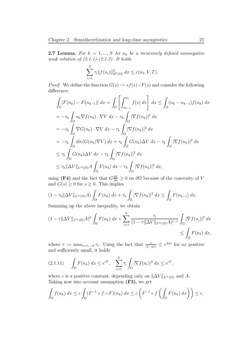
2.7 Lemma. For k = 1, ..., N let nk be a recursively defined nonnegativeweak solution of (2.1.1)-(2.1.3). It holds
N∑
i=1
τi‖f(ni)‖2H1(Ω) dx ≤ c(nI , V, T ).
Proof. We define the functionG(s) := sf(s)−F (s) and consider the followingdifference:
∫
Ω
[F (nk) − F (nk−1)] dx =
∫
Ω
[
∫ nk
nk−1
f(s) ds
]
dx ≤∫
Ω
(nk − nk−1)f(nk) dx
= −τk∫
Ω
nk∇f(nk) · ∇V dx− τk
∫
Ω
|∇f(nk)|2 dx
= −τk∫
Ω
∇G(nk) · ∇V dx− τk
∫
Ω
|∇f(nk)|2 dx
= −τk∫
Ω
div(G(nk)∇V ) dx + τk
∫
Ω
G(nk)∆V dx− τk
∫
Ω
|∇f(nk)|2 dx
≤ τk
∫
Ω
G(nk)∆V dx− τk
∫
Ω
|∇f(nk)|2 dx
≤ τk‖∆V ‖L∞(Ω)A
∫
Ω
F (nk) dx− τk
∫
Ω
|∇f(nk)|2 dx,
using (F4) and the fact that G∂V∂ν
≥ 0 on ∂Ω because of the convexity of Vand G(s) ≥ 0 for s ≥ 0. This implies
(1 − τk‖∆V ‖L∞(Ω)A)
∫
Ω
F (nk) dx+ τk
∫
Ω
|∇f(nk)|2 dx ≤∫
Ω
F (nk−1) dx.
Summing up the above inequality, we obtain
(1 − τ‖∆V ‖L∞(Ω)A)k
∫
Ω
F (nk) dx+
k∑
i=1
τi(1 − τ‖∆V ‖L∞(Ω)A)i−1
∫
Ω
|∇f(ni)|2 dx
≤∫
Ω
F (nI) dx,
where τ := maxi=1,...,k τi. Using the fact that 1(1−ax)
≤ e2ax for ax positiveand sufficiently small, it holds
∫
Ω
F (nk) dx ≤ ecT ,
k∑
i=1
τi
∫
Ω
|∇f(ni)|2 dx ≤ ecT ,(2.1.11)
where c is a positive constant, depending only on ‖∆V ‖L∞(Ω) and A.Taking now into account assumption (F3), we get∫
Ω
f(nk) dx ≤ c
∫
Ω
(F−1 f F )(nk) dx ≤ c
(
F−1 f(
∫
Ω
F (nk) dx
))
≤ c,

Chapter 2. Semidiscretization and long-time asymptotics 26
using (F2), Jensen’s inequality and the fact that f and F−1 are continuousfunctions. The Poincare inequality
k∑
i=1
τi‖f(ni) −∫
Ω
f(ni) dx‖2H1(Ω) ≤
k∑
i=1
τi‖∇f(ni)‖2L2(Ω),
and (2.1.11) finish the proof. 2
2.1.2 Existence
2.8 Lemma. Let 0 ≤ nε,k−1 ∈ L2(Ω), σ ∈ [0, 1] and 0 ≤ f(nε,k) ∈ H1(Ω),0 ≤ nε,k ∈ L2(Ω) satisfy∫
Ω
∇ψ · ∇f(nε,k) dx = − σ
∫
Ω
nε,k∇ψ · ∇V dx − σ
τk
∫
Ω
ψ(nε,k − nε,k−1) dx
− ε
∫
Ω
ψf(nε,k) dx,
for all ψ ∈ H1(Ω). It holds
N∑
i=1
τi‖f(nε,i)‖H1(Ω) ≤ ecT ,(2.1.12)
where c depends only on the initial datum nI .
Proof. Following the calculations as in Lemma 2.7, it is easy to show that∫
Ω
[F (nε,k) − F (nk−1)] dx+τkσ
∫
Ω
|∇f(nε,k)|2 dx+τkσε
∫
Ω
f(nε,k)2 dx
≤ τk‖∆V ‖L∞(Ω)A
∫
Ω
F (nε,k) dx,
using assumption (F4). Therefore, summing up in k, we obtain
(1 − τ‖∆V ‖L∞(Ω)A)k
∫
Ω
F (nε,k) dx
+k
∑
i=1
τi
(∫
Ω
|∇f(nε,i)|2 dx+ ε
∫
Ω
f(nε,i)2 dx
)
≤∫
Ω
F (nI) dx.
where τ := mini=1,..,k τi, which implies∫
Ω
F (nk) dx ≤ ecT .
Chapter 2. Semidiscretization and long-time asymptotics 27
Now, again from (F3), it holds
∫
Ω
f(nε,k) dx ≤ c
∫
Ω
(F−1 f F )(nε,k) dx ≤ c
(
F−1 f(
∫
Ω
F (nε,k) dx
))
≤ c,
using Jensen’s inequality and the fact that f and F−1 are continuous func-tions. Finally, the Poincare inequality
k∑
i=1
τi‖f(nε,i) −∫
Ω
f(nε,i) dx‖2H1(Ω) ≤
k∑
i=1
τi‖∇f(nε,i)‖2L2(Ω),
proves the lemma. 2
Proof of Theorem 2.1. We employ the Leray-Schauder theorem. Letk = 1, . . . , N be fixed and assume that 0 ≤ nk−1 ∈ L2(Ω). Moreover, letw ∈ L2(Ω) and σ ∈ [0, 1] be given and consider the problem
∫
Ω
∇ψ · ∇Fε dx = −σ∫
Ω
f−1(w+)∇ψ · ∇V dx
− σ
τk
∫
Ω
ψ(f−1(w+) − nk−1) dx− ε
∫
Ω
ψFε dx,(2.1.13)
where w+ := max(w, 0) and ψ ∈ H1(Ω).Note that, thanks to the Holder continuity property of f−1, the second andthird integral in the above equation are well-defined. Indeed, it holds, for allw ∈ L2(Ω)
∫
Ω
|f−1(w+)|2 dx =
∫
Ω
|f−1(w+) − f−1(0)|2 dx ≤ c
∫
Ω
|w+|2θ dx,
using the fact that f−1(0) = 0.Problem (2.1.13) has a unique solution Fε ∈ H1(Ω). Therefore the operatorS : L2(Ω) × [0, 1] −→ L2(Ω) given by S(w, σ) = Fε is well defined.It is easy to see that S is continuous, compact and S(w, 0) = 0 for allw ∈ L2(Ω). Let Fε ∈ H1(Ω) be a fixed-point of S, i.e. S(Fε, σ) = Fε forσ ∈ [0, 1]. We claim that Fε ≥ 0 a.e. Indeed, taking ψ = Fε
− := min(0,Fε)as test function, we get
∫
Ω
|∇Fε−|2 dx = −σ
∫
Ω
f−1(Fε+)∇Fε
− · ∇V dx
− σ
τk
∫
Ω
Fε−(f−1(Fε
+) − nk−1) dx− ε
∫
Ω
Fε−Fε dx
=σ
τk
∫
Ω
Fε−nk−1 dx− ε
∫
Ω
Fε−2
dx ≤ 0.
Chapter 2. Semidiscretization and long-time asymptotics 28
Moreover, from Lemma 2.8 we can conclude that there exists a constantC > 0 independent of σ such that ‖Fε‖H1(Ω) ≤ C for all Fε such thatS(Fε, σ) = Fε.The Leray-Schauder theorem implies that the map S(·, 1) has at least onefixed point, denoted again by Fε, which is nonnegative and solves
∫
Ω
∇ψ · ∇Fε dx = −∫
Ω
nε∇ψ · ∇V dx
− 1
τk
∫
Ω
ψ(nε − nk−1) dx− ε
∫
Ω
ψFε dx,(2.1.14)
for all ψ ∈ H1(Ω), with nε := f−1(Fε(x)).The set of functions Fε fulfills inequality (2.1.12). Therefore there existsa subsequence, denoted again with Fε, weakly convergent in H1(Ω) to Fwhen ε → 0. Moreover, from inequality (2.1.12), using again the Holder-continuity property of f−1, it holds
∫
Ω
|nε|2 dx ≤ c
∫
Ω
|Fε|2θ dx ≤ c
(
1 +
∫
Ω
|Fε|2 dx)
≤ c,
where nε(x) := f−1(Fε(x)). This implies the existence of a subsequence,denoted again by nε such that nε n weakly in L2(Ω) when ε→ 0. Passingto the limit ε → 0 in (2.1.14) it is easy to see that F and n satisfy theproblem
∫
Ω
∇ψ · ∇F dx = −∫
Ω
n∇ψ · ∇V dx
− 1
τk
∫
Ω
ψ(n− nk−1) dx− ε
∫
Ω
ψF dx.
It remains to prove that F = f(n). From the compact embeddingH1(Ω) → L2(Ω) it follows that Fε(x) → F in L2(Ω) and a.e.. Using thecontinuity property of f−1, it holds nε = f−1(Fε) → f−1(F) a.e., whichmeans n = f−1(F). This implies that n and f(n) satisfy (2.1.4). 2
Let n(N) be defined by n(N)(x, t) := nk(x) if t ∈ (tk−1, tk], x ∈ Ω and σN bethe shift operator defined as (σN(n(N)))(·, t) := nk−1 for t ∈ (tk−1, tk].
Proof of Theorem 2.2. From Corollary 2.6 and Lemma 2.7 it immedi-ately follows that the sequence (n(N))N∈N and (f(n(N)))N∈N are boundedin L∞(0, T ;L∞(Ω)) and L2(0, T ;H1(Ω)) respectively. Thus there exist sub-sequences, again denoted by (n(N)) and (f(n(N))) such that for N → +∞
n(N) n weakly in Lp(0, T ;Lp(Ω)) ∀ 1 < p < +∞,(2.1.15)
f(n(N)) f weakly in L2(0, T ;H1(Ω)).(2.1.16)

Chapter 2. Semidiscretization and long-time asymptotics 29
From (2.1.1) it holds
1
τ‖n(N) − σN(n(N))‖L2(0,T ;(H1(Ω))∗)
= ‖ sup‖v‖H1(Ω)=1
〈div(n(N)∇V + ∇f(n(N))), v〉H1∗,H1‖L2(0,T )
≤ ‖ sup‖v‖H1(Ω)=1
[
−∫
Ω
(n(N)∇V · ∇v + ∇v · ∇f(n(N))) dx
]
‖L2(0,T ) ≤ C,
using (2.1.3), which implies for N → +∞ (maybe for a subsequence)
1
τ(n(N) − σN (n(N))) nt weakly in L2(0, T, (H1(Ω))∗).(2.1.17)
Note that Corollary 2.6 and Lemma 2.7 imply also that (n(N))N∈N is uni-formly bounded in L2(0, T ;W s
p (Ω)) with 0 < s < 1, p ≥ 2 (see [29]).
It holds W sp (Ω) → W s
′
p (Ω) → L2(Ω) → (H1(Ω))∗, s′
< s, with compact
injection from W sp (Ω) into W s
′
p (Ω). From Aubin’s lemma it follows
n(N) → n strongly in L2(0, T ;W s′
p (Ω)) for N → +∞,
and maybe for a subsequence
n(N) → n a.e. for N → +∞.(2.1.18)
The above convergence and the continuity assumption on f imply f(n) = f .Finally, from Corollary 2.6 we can conclude that n ∈ L∞(0, T ;L∞(Ω)).The convergence results (2.1.15), (2.1.16) and (2.1.17) allow now to pass tothe limit N → +∞ in the weak formulation of (2.1.1) to obtain a weaksolution n and f(n) of
nt = div(n∇V + ∇f(n)), in Ω, t > 0,
such that n(·, 0) = nI in the sense of (H1(Ω))∗. 2
2.1.3 Numerical examples
The basic property of the numerical scheme (2.1.1)-(2.1.3) presented in theprevious section is the decay of the relative entropy
E(nk|n∞) :=
∫
Ω
[φ(n) − φ(n∞) − φ′(n∞)(n− n∞)] dx,(2.1.19)
where φ is a strictly convex function solving the problem
φ′′(n) =f ′(n)
n, φ′(1) = 0, φ(0) = 0,(2.1.20)

Chapter 2. Semidiscretization and long-time asymptotics 30
and n∞ := h−1(C−V (x)) the steady-state, where C is such that∫
Ωn∞ dx =
∫
ΩnI dx.
Let us also remember that for general nonlinear Fokker-Planck equations theentropy
E(nk) :=
∫
Ω
[nkV (x) + φ(nk)] dx,(2.1.21)
and the relative entropy (2.1.19) satisfy
E(nk) − E(n∞) ≥ E(nk|n∞),
being equal if and only if n∞ is positive everywhere (see [25, Proposition 5]).Moreover the difference can be explicitly written as
(2.1.22) E(nk)−E(n∞)−E(nk|n∞) =
∫
Ω
[V (x)+φ′(n∞(x))](nk −n∞)) dx.
2.9 Lemma. For k = 1, . . . , N let nk be a recursively defined nonnegativeweak solution in the sense of Theorem 2.1 of (2.1.1)-(2.1.3). Assuming that
∫
Ω
nI |∇V + ∇φ′(nI)|2 dx < +∞,(2.1.23)
it holds
E(nk) − E(n∞) ≤ (E(nI) − E(n∞))(1 + 2α∆t)−k, k ∈ N.
Proof. Here we give a formal proof of this lemma, based on the generalizedLog-Sobolev inequality (see [25, Theorem 17]). Let
D(nk) :=
∫
Ω
nk|∇V + ∇φ′(nk)|2 dx,
be the entropy production for the functional E(nk|n∞) defined in (2.1.19).Then the generalized Log-Sobolev inequality asserts that
E(nk|n∞) ≤ E(nk) − E(n∞) ≤ 1
2αD(nk) ∀ k ∈ N,(2.1.24)
using the uniform convexity of the potential V (V1). From the convexity ofφ, it follows
E(nk|n∞) ≥∫
Ω
φ′(nk+1)(nk − nk+1) + φ(nk+1) − φ(n∞) − φ′(n∞)(nk − n∞) dx
=
∫
Ω
φ(nk+1) − φ(n∞) − φ′(n∞)(nk+1 − n∞)+
+
∫
Ω
φ′(n∞)(nk+1 − nk) + φ′(nk+1)(nk − nk+1) dx
= E(nk+1|n∞) +
∫
Ω
[φ′(n∞) − φ′(nk+1)](nk+1 − nk)) dx.

Chapter 2. Semidiscretization and long-time asymptotics 31
Now, using (2.1.22) we get
E(nk) − E(n∞) ≥ E(nk+1|n∞) +
∫
Ω
[φ′(n∞) − φ′(nk+1)](nk+1 − nk)) dx
+
∫
Ω
[V (x) + φ′(n∞(x))](nk − n∞)) dx
= E(nk+1|n∞) −∫
Ω
[V (x) + φ′(nk+1)](nk+1 − nk)) dx
+
∫
Ω
[V (x) + φ′(n∞(x))](nk − n∞)) dx+
∫
Ω
φ′(n∞)(nk+1 − nk)) dx
+
∫
Ω
V (x)(nk+1 − nk)) dx
= E(nk+1|n∞) +
∫
Ω
[V (x) + φ′(n∞(x))](nk+1 − n∞)) dx
−∫
Ω
[V (x) + φ′(nk+1)](nk+1 − nk)) dx
= E(nk+1) − E(n∞) −∫
Ω
[V (x) + φ′(nk+1)](nk+1 − nk)) dx.
Therefore, from equation (2.1.1) and integrating by parts, we deduce
∫
Ω
[V (x) + φ′(nk+1)](nk+1 − nk)) dx = −∆t
∫
Ω
nk+1|∇V + ∇φ′(nk+1)|2 dx,
and thus,
E(nk) − E(n∞) ≥ E(nk+1) − E(n∞) + ∆tD(nk+1).
From inequality (2.1.24) it holds
E(nk) − E(n∞) ≥ (1 + 2α∆t) (E(nk+1) − E(n∞)),
and the theorem follows now recursively. 2
We point out that the previous lemma was already observed in the linearcase in [10] with a proof simplified by the fact V (x) + φ′(n∞(x)) = C forall x ∈ R
N for linear diffusions. It is the discrete version of the exponentialdecay with rate 2α in the continuous case obtained in [25, 27]. The rigorousproof of this lemma is done by approximations of the nonlinear function inthe same spirit as in [25].
In the case of general nonlinear diffusion equations we have also a decayestimate for the corresponding entropy.
2.10 Corollary. For k = 1, . . . , N let nk be a recursively defined nonnegativeweak solution in the sense of Theorem 2.1 of (2.1.1)-(2.1.3) with V ≡ 0,

Chapter 2. Semidiscretization and long-time asymptotics 32
f(n) = nm and
E(k) :=
∫
Ω
φ(nk(x)) dx.(2.1.25)
For all k ∈ N it holds
E(k) ≥ E(k + 1).
Let us show some numerical results related to problem (2.1.1) in the casef(n) := nm for some m > 1.
The porous medium equation.
We introduce the fully discretization of equation (2.1.1) with V ≡ 0 in auniform grid using central finite differences in space to obtain:
nk(i) − nk−1(i)
∆t= D+D−(f(nk(i))), k ∈ N, i = 1, . . . ,M,
where D+ and D− are the standard forward and backward first order fi-nite difference operators, defined for any discretized function (z(i))i=1,...,M asfollows
D+z(i) :=z(i + 1) − z(i)
∆x, i = 1, . . . ,M − 1,
D−z(i) :=z(i) − z(i − 1)
∆x, i = 2, . . . ,M.
The resulting nonlinear system of equations is iteratively solved by Newton’smethod at each time step. Time stepping is set to constant.
Figure 2.1 shows numerical results for f(n) := n2 with initial data
(2.1.26) nI(x) =
2[(4−x2)−3.9 cos(π4x)]
‖2[(4−x2)−3.9 cos(π4x)]‖L1(−2,2)
if − 2 ≤ x ≤ 2,
0 otherwise.
Let us point out that the expected Barenblatt asymptotic profile
B(|x|, t) = t−dλ
(
C − (m− 1)
2mλ|x|2t− 2
λ
)1
m−1
+
,(2.1.27)
is fixed by mass conservation∫
R
B(|x|, t) dx =
∫
R
nI(x) dx.

Chapter 2. Semidiscretization and long-time asymptotics 33
(a)
−8 −6 −4 −2 0 2 4 6 80
0.05
0.1
0.15
0.2
0.25
0.3
0.35
x
n(x,
t)
v2(x,t) : solution of the p.m. equation
t=0t=5⋅ 10−1
t=5t=20
(b)
0 5 10 15 200.1
0.15
0.2
0.25
0.3
0.35
t
Ent
ropy
Figure 2.1: Numerical results and entropy decay for (2.1.1) in case f(n) = n2 and
V ≡ 0 with initial condition (2.1.26) (a) Time evolution of n(x, t), (b) Entropy
evolution E(t).
The results show the convergence to the selfsimilar profile given by the Baren-blatt profile (2.1.27), where λ := d(m − 1) + 2 and m = 2 in this case, ast → ∞ and the decreasing character of the entropy. Note that in this casethe decay rate of the entropy is not exponential but rather algebraic. In fact,for the porous medium equation the entropy becomes the Lm of the solutionthat decays like m−1
mλ due to the L1-L∞ effect [11] which asserts
‖n(·, t)‖L∞(Rd) ≤ C t−d
d(m−1)+2 ‖nI‖L1(Rd).
In figure 2.2 the numerical approximations of the two dimensional porousmedium equation with f(n) = n3 together with the entropy decay are plotted.
Nonlinear Fokker-Planck equation
This part of the work is devoted to the investigation of problem (2.1.1) incase f(n) := nm, m > 1 and V (x) := 1
2x2. It is well known that a standard
central finite differences fully discretized implicit Euler scheme for (2.1.1)does not give nice results. This is due to the fact that if |Vx| assumes largevalues where the function n is small, the drift term nVx becomes predominantwith respect to the diffusion term f(n)xx will cause undesired oscillations andlarge negative values in the solution (see figure 2.3).
Therefore we follow the same scheme as in [48], used for a numerical approx-imation of the one dimensional transient drift-diffusion model for a bipolarsemiconductor.
We recall briefly the most important steps. For the space discretization,we make use of a mixed exponential fitting method. The main idea con-

Chapter 2. Semidiscretization and long-time asymptotics 34
−2
−1
0
1
2
−2
−1
0
1
2
0
0.02
0.04
0.06
0.08
0.1
0.12
0.14
y
t=0
x−2
−1
0
1
2
−2
−1
0
1
2
0
0.005
0.01
0.015
0.02
0.025
0.03
y
t=1.4
x
−2
−1
0
1
2
−2
−1
0
1
2
0
0.002
0.004
0.006
0.008
0.01
0.012
0.014
0.016
y
t=4.2
x
−2
−1
0
1
2
−2
−1
0
1
20
0.002
0.004
0.006
0.008
0.01
0.012
y
t=11
x
z
0 2 4 6 8 10 120
1
2
3
4
5
6
7x 10
−3
t
Entropy
Figure 2.2: Time evolution and Entropy decay of the 2D nonlinear diffusionequation (2.1.1) with f(n) = n3 and V ≡ 0.
sists to linearize at each time step the current of the equation assum-ing f ′(n(x, tk)) ∼ f ′
k(x) is already known and rewrite the current termJ(x, t) := −(n(x, t)Vx(x) + f ′
k(x)nx(x, t)) into an equation for the new vari-able z := ne−V in each spatial cell.
Let xi = i∆x, where i = 1, . . . ,M and ∆x > 0, Ii := (xi−1, xi] and Jk(i),nk(i) and V (i) be denote the approximative term on xi at time tk := k∆t.The method can be summarized in two main steps: (1) approximation of thediffusion term , (2) change of variable.
It makes physically sense to expect that, if the current density Jk in the

Chapter 2. Semidiscretization and long-time asymptotics 35
−1 −0.5 0 0.5 1−0.2
−0.1
0
0.1
0.2
0.3
0.4
0.5
0.6
0.7
0.8
x
n(x,
t)
t=0t=8⋅ 10−3
t=24⋅ 10−3
t=32⋅ 10−3
Figure 2.3: Numerical results of (2.1.1) with central finite differences.
interval Ii is positive, the flow is moving to the right direction and then thedensity valuated at the left nk(i− 1) can be taken for the approximation ofthe coefficient of the diffusion term. More precisely
f ′k(i) :=
f ′(nk(i− 1)) if Jk(i) > 0,
f ′(nk(i)) if Jk(i) ≤ 0,(2.1.28)
where we need an approximated value of the current Jk(i) in Ii, for this, wetake
Jk(i) :=
0 if nk(i) = nk(i− 1) = 0,−1∆x
[(φ′(nk(i)) − φ′(nk(i− 1))) + (V (i) − V (i− 1))] else.
We define now a new variable
zk := nk exp(V/f ′k(i)) in Ii.
Then the expression of the current on the interval Ii becomes
Jk ' −(f ′k(i) exp(−V/f ′
k(i))zk,x))
and equation (2.1.1) can be rewritten as
1
f ′k(i)
exp(V/f ′k(i))Jk + zk,x = 0 in Ii,
(Jk)x = − 1
∆t(nk+1 − nk) in Ii.
We approximate now Jk and zk as follows
Jk ∈ X1 := ω ∈ L2(Ω) | ω(x) = aix + bi, x ∈ Ii, i = 1, . . . ,M,zk ∈ X0 := ξ ∈ L2(Ω) | ξ const. in Ii, i = 1, . . . ,M,

Chapter 2. Semidiscretization and long-time asymptotics 36
and taking ω ∈ X1 and ξ ∈ X0 as test functions for the above equations, thediscrete system becomes
M∑
i=1
(∫
Ii
1
f ′k(i)
exp(V/f ′k(i))Jkω dx−
∫
Ii
zkωx dx+ [uk exp(V/f ′k(i))ω]xi
xi−1
)
= 0,
M∑
i=1
(∫
Ii
(Jk)xξ +
∫
Ii
1
∆t(nk+1 − nk)ξ
)
= 0.
We have now to approximate the last integrals. We choose ξ = 1 in Ii andξ = 0 elsewhere as test function, getting in this way
Jk(i) − Jk(i− 1) = − 1
∆t
∫
Ii
(nk+1 − nk).
The last integral is approximated as follows
∫
Ii
(nk+1 − nk) = ∆x(nk+1(i− 1) − nk(i− 1)).
It remains to compute Jk; first we approximate Jk(x) = Jk(i) if x ∈ Ii, thentaking ω = 1 in Ii and ω = 0 elsewhere as test function, it holds
∫
Ii
1
f ′k(i)
exp(V/f ′k(i))Jk(i) dx = −[nk exp(V/f ′
k(i))]xixi−1
,
which implies
Jk(i) = −(
V (i) − V (i− 1)
2coth
V (i) − V (i− 1)
2f ′k(i)
)
nk(i) − nk(i− 1)
∆x
− nk(i) + nk(i− 1)
2
V (i) − V (i− 1)
∆x.
This approximation for the flux is used in combination with an explicit Eulermethod
nk+1(i) − nk(i)
∆t= − 1
∆x(Jk(i+ 1) − Jk(i)).
Since the approximation for the flux is conservative, it is clear that the L1
norm of the solution will be preserved at the fully discrete level.
Figure 2.4 shows the evolution in time of (2.1.1) with f(n) = n2. In this casethe stationary-state of the problem with initial data
(2.1.29) nI(x) =
π4
cos(
π2x)
if − 1 ≤ x ≤ 1,0 otherwise,
Chapter 2. Semidiscretization and long-time asymptotics 37
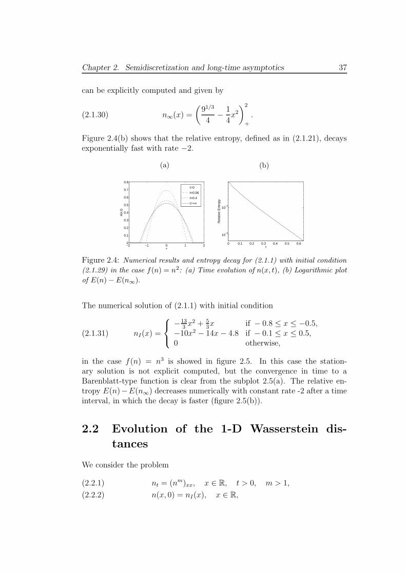
can be explicitly computed and given by
n∞(x) =
(
91/3
4− 1
4x2
)2
+
.(2.1.30)
Figure 2.4(b) shows that the relative entropy, defined as in (2.1.21), decaysexponentially fast with rate −2.
(a)
−2 −1 0 1 20
0.1
0.2
0.3
0.4
0.5
0.6
0.7
0.8
x
n(x,
t)
t=0
t=0.06
t=0.4
t=+∞
(b)
0 0.1 0.2 0.3 0.4 0.5 0.6
10−3
10−2
Rel
ativ
e E
ntro
py
t
Figure 2.4: Numerical results and entropy decay for (2.1.1) with initial condition
(2.1.29) in the case f(n) = n2: (a) Time evolution of n(x, t), (b) Logarithmic plot
of E(n) − E(n∞).
The numerical solution of (2.1.1) with initial condition
(2.1.31) nI(x) =
−133x2 + 5
3x if − 0.8 ≤ x ≤ −0.5,
−10x2 − 14x− 4.8 if − 0.1 ≤ x ≤ 0.5,0 otherwise,
in the case f(n) = n3 is showed in figure 2.5. In this case the station-ary solution is not explicit computed, but the convergence in time to aBarenblatt-type function is clear from the subplot 2.5(a). The relative en-tropy E(n)−E(n∞) decreases numerically with constant rate -2 after a timeinterval, in which the decay is faster (figure 2.5(b)).
2.2 Evolution of the 1-D Wasserstein dis-
tances
We consider the problem
nt = (nm)xx, x ∈ R, t > 0, m > 1,(2.2.1)
n(x, 0) = nI(x), x ∈ R,(2.2.2)
Chapter 2. Semidiscretization and long-time asymptotics 38
(a)
−1.5 −1 −0.5 0 0.5 1 1.50
0.2
0.4
0.6
0.8
1
1.2
1.4
1.6
x
t=0t=0.026t=0.1t=0.5
(b)
0 0.1 0.2 0.3 0.4 0.510
−6
10−4
10−2
100
102
t
Figure 2.5: Numerical results and entropy decay for (2.1.1) with initial condition
(2.1.31) in the case f(n) = n3: (a) Time Evolution of n(x, t), (b) Logarithmic plot
of E(n) − E(n∞) .
where nI ∈ L1(R) ∩ L∞(R), ‖nI‖L1(R) = 1, nI ≥ 0 and nI is compactlysupported.
Much is already known for problem (2.2.1), (2.2.2): see [27, 57, 76, 74, 75]and the references therein for existence, uniqueness and asymptotic behaviourresults of the porous media equation. It also known that the degeneracy atlevel n = 0 of the diffusivity D(n) = mnm−1 causes the phenomenon calledfinite speed of propagation. This means that the support of the solution n(·, t)to (2.2.1), (2.2.2) is a bounded set for all t ≥ 0. In fact it can be provedthat the solution n(x, t) as t→ +∞ converges to the Barenblatt source-typesolution B(|x|, t, C) with the same mass as the initial data.In this paper we want to give a simple proof of the finite propagation propertyusing mass transportation techniques. Precisely, we prove that the differenceof support of two solutions of (2.2.1), (2.2.2) with different compactly sup-ported initial conditions is a bounded in time function of a suitable Monge-Kantorovich related metric.
2.11 Theorem. Let n1(x, t) and n2(x, t) be strong solutions of (2.2.1)-(2.2.2)with initial conditions nI1(x) and nI2(x) respectively, where nI i ∈ L1(R) ∩L∞(R), ‖nI i‖L1(R) = 1, nI i ≥ 0 and nI i is compactly supported, i = 1, 2, andlet Ωi(t) = x ∈ R/ni(x, t) > 0 , i = 1, 2.
Let ξi(t) = inf[Ωi(t)], Ξi(t) = sup[Ωi(t)], for t ≥ 0, i = 1, 2. Then
max |ξ1(t) − ξ2(t)|, |Ξ1(t) − Ξ2(t)| ≤ W∞(nI1, nI2), ∀t ∈ [0,+∞),
where W∞(nI1, nI2) is a constant, which depends only on the initial datanI1, nI2 and is defined in (2.2.14).
The finite speed of propagation property follows by just taking as one ofthe solutions a time translation of the explicit Barenblatt solution which isknown to have compact support expanding at the rate t1/(m+1).

Chapter 2. Semidiscretization and long-time asymptotics 39
Proof. Consider a sequence of functions nk ∈ C∞([0,+∞) × R), which arestrong solutions (see [75]) of the problems Pk
nt = (nm)xx, x ∈ R, t > 0, m > 1,(2.2.3)
n(x, 0) = nIk(x), x ∈ R,(2.2.4)
where nIk(x), k ∈ N, is a sequence of bounded, integrable and strictly positiveC∞-smooth functions such that all their derivatives are bounded in R, thecondition (m−1)(nI
mk )xx ≥ −anIk holds for some constant a > 0, and nIk →
nI in L1(R) if k → +∞. We may always do it in such a way that ‖nIk‖L1(R) =‖nI‖L1(R) and ‖nIk‖L∞(R) ≤ ‖nI‖L∞(R). From the L1-contraction property itfollows that nk → n in C([0,+∞) : L1(R)) if k → +∞, where n is astrong solution of (2.2.1)-(2.2.2) (see [75], chapt. III).
This sequence of regularized solutions can be further approximated by asequence of initial boundary value problems. We introduce a cutoff sequenceθl ∈ C∞(R), 1 < l ∈ N, with the following properties:
θl(x) = 1 for |x| < l − 1,
θl(x) = 0 for |x| ≥ l, 0 < θl < 1 for l − 1 < |x| < l.
The initial boundary value problem Pkl
nt = (nm)xx, x ∈ (−l, l), t > 0,(2.2.5)
n(x, 0) = nIkl(x) :=nIk(x)θl(x)
‖nIk(x)θl(x)‖L1
,(2.2.6)
n(x, t) = 0 for |x| = l, t ≥ 0,(2.2.7)
is mass preserving and has a unique solution nkl(x, t) ∈ C∞((0,+∞) ×[−l, l]) ∩ C([0,+∞) × [−l, l]), strictly positive for x ∈ (−l, l) and zero atthe boundary (see [75], prop.6, chapt.II). Because nIkl −→ nIk as l −→ +∞,for all k ∈ N, nkl → nk in C([0,+∞) : L1(R)) if l → +∞, where nk issolution of the problem Pk.
Thanks to estimates independent of l for the moments of the solutions ofthe Pkl problems and passing to the limit in the corresponding inequalities,it can be easily shown that the solution nk(x, t) of (2.2.3)-(2.2.4) enjoys animportant property. It holds
∫
R
|x|pnk(x, t)dx < +∞, ∀t ≥ 0, ∀p ∈ [1,+∞).(2.2.8)
We shall denote by Pp(R), with p ∈ [1,+∞), the set of all probability mea-sures on R with finite moments of order p. Let Π(µ, ν) be the set of allprobability measures on R
2 having µ, ν ∈ Pp(R) as marginal distributions

Chapter 2. Semidiscretization and long-time asymptotics 40
(see [77]). The Wasserstein p-distance between two probability measuresµ, ν ∈ Pp(R) is defined as
Wp(µ, ν)p := inf
π∈Π(ν,µ)
∫
R2
|x− y|pdπ(x, y), ∀p ∈ [1,+∞).(2.2.9)
Wp defines a metric on Pp(R) (see [77]). Bound (2.2.8) then shows that theWasserstein p-distance between any two solutions which is initially finite, re-mains finite at any subsequent time.Any probability measure µ on the real line can be described in terms of its cu-mulative distribution function F (x) = µ((−∞, x]) which is a right-continuousand non-decreasing function with F (−∞) = 0 and F (+∞) = 1. Then, thegeneralized inverse of F defined by F−1(η) = infx ∈ R/F (x) > η is alsoa right-continuous and non-decreasing function on [0, 1].Let µ, ν ∈ Pp(R) be probability measures and let F (x), G(x) be the re-spective distribution functions. On the real line (see [77]), the value of theWasserstein p-distance Wp(µ, ν) can be explicitly written in terms of thegeneralized inverse of the distribution functions,
Wp(µ, ν)p =
∫ 1
0
|F−1(η) −G−1(η)|pdη, ∀p ∈ [1,+∞).(2.2.10)
Let n1(x, t), n2(x, t) be strong solutions of (2.2.1), (2.2.2) corresponding toinitial conditions nI1(x) and nI2(x) respectively. We denote by n1k(x, t)and n2k(x, t) the strong solutions of (2.2.3), (2.2.4) with initial conditionsnI1k(x) and nI2k(x) respectively, where nI ik −→ nI i in L1(R) for i = 1, 2.Analogously, we consider the solutions n1kl(x, t) and n2kl(x, t) of the problemsPkl converging towards nik(x, t) for i = 1, 2 in C([0,+∞) : L1(R)) as l → ∞.Let Fikl(x, t) be the distribution functions of nikl for i = 1, 2. A directcomputation shows that Fi
−1kl (η, t) solves the following equation
∂Fi−1kl
∂t= − ∂
∂η
((
∂Fi−1kl
∂η
)−m)
, i = 1, 2,(2.2.11)
for t > 0 and η ∈ [0, 1]. Making use of equation (2.2.11), it is easy to provethat the Wasserstein p-distance
Wp(n1kl, n2kl)(t) =
∫ 1
0
|F1−1kl (η, t) − F2
−1kl (η, t)|pdη
1p
, ∀p ∈ [1,+∞),
is a non-increasing in time function. In fact, for any given p ≥ 1, integratingby parts one obtains
d
dt
∫ 1
0
|F1−1kl (η, t) − F2
−1kl (η, t)|pdη = p(p− 1)
∫ 1
0
|F1−1kl (η, t) − F2
−1kl (η, t)|p−2
×(
F1−1kl (η, t)η − F2
−1kl (η, t)η
)
[
(
F1−1kl (η, t)η
)−m −(
F2−1kl (η, t)η
)−m]
dη ≤ 0

Chapter 2. Semidiscretization and long-time asymptotics 41
since the function x−m, m ≥ 1, is decreasing. Note that the boundary termsvanish due to the compact support of the solutions, which implies
limη→0+
(
Fi−1kl (η, t)η
)−1= lim
η→1−
(
Fi−1kl (η, t)η
)−1= 0 i = 1, 2.
On the other hand, for all p ∈ [1,+∞),
Wp(n1kl, n2kl) → Wp(n1k, n2k), l → +∞,(2.2.12)
Wp(n1k, n2k) →Wp(n1, n2), k → +∞.(2.2.13)
This implies that Wp(n1, n2) ≤ Wp(nI1, nI2), ∀p ∈ [1,+∞). Since the func-tion Wp(n1, n2) is increasing with respect to p, we can define the quantity
W∞(n1, n2) := limp↑+∞
Wp(n1, n2)
= supη∈(0,1)
ess|F−11 (η, t) − F−1
2 (η, t)|.(2.2.14)
Since W∞(nI1, nI2) is finite, we deduce easily that W∞(n1, n2) is also a non-increasing in time function.Note that the inverse function F−1(η) of a distribution F (x) =
∫ x
−∞ n(s)ds,where n(s) is a integrable compactly supported function, is continuous at thepoint η = 0 and η = 1. Thus we can justify the inequality
W∞(n1, n2) = supη∈(0,1)
ess|F−11 (η, t) − F−1
2 (η, t)|
≥ max
|F−11 (0, t) − F−1
2 (0, t)|, |F−11 (1, t) − F−1
2 (1, t)|
≥ max |ξ1(t) − ξ2(t)|, |Ξ1(t) − Ξ2(t)| .(2.2.15)
2
We remark that the above arguments only hold in one space dimension dueto the fact that only in this case one can express the p-Wasserstein distancein terms of pseudo-inverse distribution functions, as given in (2.2.10).
Figure 2.6 shows the evolution of the p-Wasserstein distance defined in(2.2.10) for several values of p between n1(x, t) and n2(x, t), solutions of(2.2.1), (2.2.2) with initial conditions (2.1.26) and (2.1.29) respectively, incase m = 2. The integral in (2.2.10) for the forthcoming tests is computedby numerical quadrature and we are using the fully discretized implicit Eulerscheme described in subsection 2.1.
It is interesting to observe that although the distance between the solutionsis only known to be a contraction, this distance is in fact decaying quickly ast → ∞. Let us point out that the two initial data have zero center of massand therefore are well centered. In fact, it is a conjecture to prove that thereis a decay of the distance between the solutions when you fix the center ofmass of the initial data. In the case of expansion rate of supports, this wasalready observed by J. L. Vazquez in [74].

Chapter 2. Semidiscretization and long-time asymptotics 42
(a)
0 5 10 15 200
0.1
0.2
0.3
0.4
0.5
0.6
0.7
0.8
t
p=2
(b)
0 5 10 15 200.1
0.2
0.3
0.4
0.5
0.6
0.7
0.8
0.9
t
p=5
(c)
0 5 10 15 200.1
0.2
0.3
0.4
0.5
0.6
0.7
0.8
0.9
t
p=15
Figure 2.6: Time evolution of the Wasserstein p-metric Wp(n1, n2), where n1(x, t)
and n2(x, t) are solutions of (2.2.1), (2.2.2) with m = 2 and initial conditions
(2.1.26) and (2.1.29) respectively, in case (a) p = 2, (b) p = 5, (c) p = 15.

Chapter 3
Analysis of the viscousquantumhydrodynamicequations
The objective of this chapter is the analysis to the one-dimensional stationaryviscous quantum hydrodynamic model
Jx = νnxx,(3.0.1)(
J2
n
)
x
+ Tnx − nVx =ε2
2n
(
(√n)xx√n
)
x
− J
τ+ νJxx,(3.0.2)
λ2Vxx = n− C(x) in (0, 1).(3.0.3)
subject to the boundary conditions
n(0) = n(1) = 1, nx(0) = nx(1) = 0, V (0) = V0,(3.0.4)
J(0) = J0, V0 = −(
2ν2 +ε2
2
)
(√n)xx(0) +
J20
2.(3.0.5)
The last boundary condition can be interpreted as a Dirichlet condition forthe Bohm potential at x = 0. Indeed, as the electrostatic potential is onlydefined up to an additive constant, this constant can be chosen such that(√n)xx(0) = α holds for any α ∈ R (often α = 0, see, e.g., [53]). Notice that
we prescribe the current density but not the applied voltage V (1) − V (0).Given J0, the applied voltage can be computed from the solution of the aboveboundary-value problem, which gives a well-defined current-voltage charac-teristic.Equations (3.0.1)-(3.0.3) can be derived from the Wigner-Fokker-Planckequations (1.0.4) with collision operator Q(w) defined as (1.0.5) by a mo-ment method, taking as closure condition an O(ε4) approximation of the
43
Chapter 3. Analysis of the viscous quantum hydrodynamic equations 44
thermal equilibrium density.As we mention in the introduction, the system (3.0.1)-(3.0.3) can be refor-mulated as an elliptic fourth-order equation for the electron density n: afterintegration of (3.0.1) and substitution into (3.0.2) we obtain the expression(1.2.4). When we divide (1.2.4) by n and differentiate with respect to x, thisequation is formally equivalent to
−(
2ν2 +ε2
2
) (
(√n)xx√n
)
xx
+(
T +ν
τ
)
(logn)xx
=n− C
λ2+ J2
0
(nx
n3
)
x− 2J0ν
(
1
n(log n)xx
)
x
− J0
τ
(
1
n
)
x
,(3.0.6)
using Poisson equation (3.0.3). The electrostatic potential can be recoveredfrom (1.2.4), after division by n and integration:
V (x) = −(
2ν2 +ε2
2
)
(√n)xx√n
(x) +(
T +ν
τ
)
log n(x) +J2
0
2n(x)2
+J0
τ
∫ x
0
ds
n(s)+ 2J0ν
nx
n2(x) + 2J0ν
∫ x
0
n2x
n3ds.(3.0.7)
The integration constant vanishes due to the boundary condition (3.0.5). Themain difficulties in the analysis of equation like (3.0.6) are the mathematicaltreatment of the fourth and third order terms and the proof of positivity forthe particle density. In this case the maximum principle is not available andother techniques are required. We note that the fourth-order term can berewritten as
(
n
(
(√n)xx√n
)
x
)
x
=1
2(n(logn)xx)xx.
This reformulation suggests to introduce the exponential variable n = eu;in fact in one space dimension an H1 estimate for u yields L∞ bound andhence positivity for the function n. Setting n = eu in (3.0.6) we arrive to theproblem
−(
ν2 +ε2
4
) (
uxx +u2
x
2
)
xx
+(
T +ν
τ
)
uxx
= λ−2(eu − C) + J20 (e−2uux)x − 2J0ν(e
−uuxx)x −J0
τ(e−u)x,(3.0.8)
V (x) = −(
ν2 +ε2
4
) (
uxx +u2
x
2
)
(x) +(
T +ν
τ
)
u(x) +J2
0
2e−2u(x)
+J0
τ
∫ x
0
e−u(s)ds+ 2J0νe−u(x)ux(x) + 2J0ν
∫ x
0
e−uu2xds.(3.0.9)
Equation (3.0.8) has to be solved in the interval (0, 1) with the boundaryconditions
(3.0.10) u(0) = u(1) = 0, ux(0) = ux(1) = 0.

Chapter 3. Analysis of the viscous quantum hydrodynamic equations 45
The problems (3.0.1)-(3.0.5) and (3.0.8)-(3.0.10) are equivalent for classicalsolutions if n > 0 in (0, 1). Indeed, we have already shown that a classicalsolution to (3.0.1)-(3.0.5) with n > 0 in (0, 1) provides via u = log n aclassical solution to (3.0.8)-(3.0.10). Conversely, let (u, V ) be a classicalsolution to (3.0.8)-(3.0.10). Setting n = eu gives n > 0 in (0, 1), and theequations (3.0.6) and (3.0.7) hold. Differentiating (3.0.7) twice, multiplyingby n and comparing with (3.0.6) yields the Poisson equation (3.0.3). Then,differentiating (3.0.7) once and multiplying the resulting equation by n, weobtain (3.0.2). Finally, the boundary condition (3.0.5) follows from (3.0.7)using (3.0.4). Thus it is sufficient to prove the existence of solutions to(3.0.8)-(3.0.10).Our results can be easily extended to Dirichlet boundary conditionsn(0) 6= n(1), following the technique used in [44], but we use (3.0.4) for thesake of a smoother presentation.
Our existence result is as follows.
3.1 Theorem (Existence and uniqueness). Let C ∈ L∞(0, 1), C > 0 in(0, 1), 0 < γ < 1, and
(3.0.11) 0 < J0 ≤γ√2e−M(γ)
√
T +ε2
16+ν
τ,
where the constant M(γ) > 0 is defined in (3.1.5). Then there exists aclassical solution (n, J, V ) to (3.0.1)-(3.0.5) such that n(x) ≥ e−M(γ) > 0 forx ∈ (0, 1). Furthermore, if J0 and ν2 + ε2 are sufficiently small, the problem(3.0.1)-(3.0.5) has a unique solution.
The restriction (3.0.11) implies (1.2.3) since
J0
n≤ J0e
M(γ) <1√2
√
T +ε2
16+ν
τ.
The constant γ needs to be smaller than one since M(γ) → ∞ for γ → 1such that γe−M(γ) → 0.
We are able to prove the semiclassical limit ε → 0, the inviscid limit ν →0 and the combined semiclassical-inviscid limit ε → 0 and ν → 0. Werefer to the appendix for the physical assumptions on the parameters, whichcorrespond to such limits.
3.2 Theorem (Inviscid limit). Let (nν , Jν, Vν) be a solution to (3.0.1)-(3.0.5) and assume that condition (3.0.11) holds for ν = 0. Then, as ν → 0,
Chapter 3. Analysis of the viscous quantum hydrodynamic equations 46
maybe for a subsequence,
nν n weakly in H2(0, 1),
Vν V weakly in H4(0, 1),
Jν J weakly in H1(0, 1),
and (n, J, V ) is a (classical) solution of the quantum hydrodynamic equations
(
J2
n+ Tn
)
x
− nVx −ε2
2n
(
(√n)xx√n
)
x
= −Jτ,
J = J0, λ2Vxx = n− C in (0, 1),
n(0) = n(1) = 1, nx(0) = nx(1) = 0, V (0) = V0.
3.3 Theorem (Semiclassical limit). Let (nε, Jε, Vε) be a solution to(3.0.1)-(3.0.5) and assume that condition (3.0.11) holds for ε = 0. Then, asε→ 0, maybe for a subsequence,
nε n weakly in H2(0, 1),
Vε V weakly in H4(0, 1),
Jε J weakly in H1(0, 1),
and (n, J, V ) is a (classical) solution of
(
J2
n+ Tn
)
x
− nVx = νJxx −J
τ, Jx = νnxx, λ2Vxx = n− C in (0, 1),
n(0) = n(1) = 1, nx(0) = nx(1) = 0, V (0) = V0, J(0) = J0.
3.4 Theorem (Semiclassical-inviscid limit). Let δ = ν2 + ε2/4, V0 =J2
0/2, let (nδ, Jδ, Vδ) be a solution to (3.0.1)-(3.0.5), and assume that condi-tion (3.0.11) holds for δ = 0. Then, as δ → 0, maybe for a subsequence (seeRemark 3.11),
nδ n weakly in H1(0, 1),(3.0.12)
Vδ V weakly in H3(0, 1),(3.0.13)
Jδ J weakly in H1(0, 1),(3.0.14)
and (n, J, V ) is a (classical) solution of the hydrodynamic equations
(
J2
n+ Tn
)
x
− nVx = −Jτ, J = J0, λ2Vxx = n− C,(3.0.15)
n(0) = n(1) = 1, V (0) = V0.(3.0.16)
Chapter 3. Analysis of the viscous quantum hydrodynamic equations 47
3.5 Remark. The convergence results for the electron density are not strongenough to conclude that the boundary condition (3.0.5) holds. However, theboundary conditions of the limit equations are sufficient to get (formally)well-posed problems.
In section (3.1) we show existence of solution to (3.0.1)-(3.0.5); the proof oftheorem (3.1) is completed in section (3.2), where the uniqueness of solutionis proved. Finally the inviscid and semiclassical limits (theorem (3.2), (3.3)and (3.4)) are performed in section (3.3) and the last part of the chapterconcerns a sketch of the derivation of model and its scaling.
3.1 Existence of solutions
As usual, we call u ∈ H20 (0, 1) a weak solution of (3.0.8), (3.0.10) if for all
ψ ∈ H20 (0, 1) it holds
−(
ν2 +ε2
4
)∫ 1
0
(
uxx +1
2u2
x
)
ψxxdx−(
T +ν
τ
)∫ 1
0
uxψxdx(3.1.1)
= 2J0ν
∫ 1
0
uxxe−uψxdx− J2
0
∫ 1
0
uxe−2uψxdx
+J0
τ
∫ 1
0
e−uψxdx+1
λ2
∫ 1
0
(eu − C)ψdx.
In order to prove Theorem 3.1 we consider the following truncated problem:
−(
ν2 +ε2
4
)∫ 1
0
(
uxx +1
2u2
x
)
ψxxdx−(
T +ν
τ
)∫ 1
0
uxψxdx
= 2J0ν
∫ 1
0
uxxe−uMψxdx− J2
0
∫ 1
0
uxe−2uMψxdx
+J0
τ
∫ 1
0
e−uψxdx+1
λ2
∫ 1
0
(eu − C)ψdx,(3.1.2)
where M = M(γ) > 0 is the constant from (3.0.11) defined in (3.1.5) belowand
uM =
u if |u| ≤MMsign(u) otherwise.
The following lemma is the key result of this part.
3.6 Lemma. (H2-Estimate). Let u ∈ H20 (0, 1) be a solution of (3.1.2) and
let (3.0.11) hold for some 0 < γ < 1. Then
(3.1.3)
(
ν2 +ε2
4
)
‖uxx‖2L2 +
(
T +ν
τ
)
‖ux‖2L2 ≤ K(γ),
Chapter 3. Analysis of the viscous quantum hydrodynamic equations 48
where K(γ) > 0 is independent of u, ν, and ε (see (3.1.7) for its definition).In particular, it follows
(3.1.4) ‖u‖L∞ ≤M(γ),
where
(3.1.5) M(γ) =
√
K(γ)
T.
Proof. We use ψ = u as a test function in the weak formulation of (3.1.2) toobtain
(
ν2 +ε2
4
)∫ 1
0
(
u2xx +
1
2u2
xuxx
)
dx+
(
T +ν
τ
)∫ 1
0
u2xdx
= −2J0ν
∫ 1
0
uxxe−uMuxdx+ J2
0
∫ 1
0
u2xe
−2uMdx
−J0
τ
∫ 1
0
e−uuxdx−1
λ2
∫ 1
0
u(eu − C)dx
= I1 + I2 + I3 + I4.(3.1.6)
We estimate the right-hand side term by term. By Young’s inequality,
I1 = −2J0ν
∫ 1
0
uxxe−uMuxdx ≤ 2J0e
Mν
∫ 1
0
|uxx||ux|dx
≤ (1 − η)ν2
∫ 1
0
u2xxdx+
J20 e
2M
1 − η
∫ 1
0
u2xdx,
where 0 < η < (1 − γ2)/(1 − γ2/2). Furthermore,
I2 = J20
∫ 1
0
u2xe
−2uMdx ≤ J20e
2M
∫ 1
0
u2xdx.
Due to the boundary conditions (3.0.10), the third integral vanishes: I3 = 0.It is not difficult to see that 1/e + ‖C logC‖L∞ is an upper bound for thefunction u 7→ −u(eu − C(x)), u ∈ R, for any x ∈ (0, 1). Here we use theassumption that the concentration C(x) is positive. Therefore,
I4 ≤ λ−2(e−1 + ‖C logC‖L∞).
Noticing that the integral
∫ 1
0
u2xuxxdx =
1
3(u3
x(1) − u3x(0)) = 0
Chapter 3. Analysis of the viscous quantum hydrodynamic equations 49
vanishes, due to the boundary conditions (3.0.10), we conclude that (3.1.6)can be estimated as(
ην2 +ε2
4
)
‖uxx‖22 +
(
T +ν
τ− 2 − η
1 − ηJ2
0e2M
)
‖ux‖22 ≤ λ−2(e−1+‖C logC‖L∞).
In view of condition (3.0.11) we obtain
T +ν
τ− 2 − η
1 − ηJ2
0 e2M ≥
(
1 − 2 − η
1 − η
γ2
2
)(
T +ν
τ
)
− 2 − η
1 − η
γ2
2
ε2
16.
Using the Poincare inequality
ε2
16
∫ 1
0
u2xdx ≤ ε2
4
∫ 1
0
u2xxdx,
this gives
[
ην2 +
(
1 − γ2(2 − η)
2(1 − η)
)
ε2
4
]
‖uxx‖2L2 +
(
1 − γ2(2 − η)
2(1 − η)
)(
T +ν
τ
)
‖ux‖2L2
≤ λ−2(e−1 + ‖C logC‖L∞)
or(
ν2 +ε2
4
)
‖uxx‖2L2 +
(
T +ν
τ
)
‖ux‖2L2 ≤ K(γ),
where
(3.1.7) K(γ) =1
λ2
(
1
e+ ‖C logC‖L∞
)
min
η, 1 − γ2(2 − η)
2(1 − η)
−1
.
Notice that 1−γ2(2− η)/(2(1− η)) > 0 due to the choice of η. Finally, fromthe Poincare-Sobolev estimate,
‖u‖L∞ ≤ ‖ux‖L2 ≤M(γ),
where M(γ) =√
K(γ)/T . This proves the lemma. 2
3.7 Lemma. Under the assumptions of Lemma 3.6, there exists a solutionu ∈ H2
0 (0, 1) of (3.1.1).
Proof. The existence of a solution of the problem (3.1.1) is shown by usingthe Leray-Schauder fixed-point theorem. For this, we consider the followinglinear problem for given w ∈ H1
0 (0, 1) with test functions ψ ∈ H20 (0, 1):
(3.1.8) −a(u, ψ) = σF (ψ),
Chapter 3. Analysis of the viscous quantum hydrodynamic equations 50
where σ ∈ [0, 1],
(3.1.9) a(u, ψ) =
(
ν2 +ε2
4
)∫ 1
0
uxxψxxdx +
(
T +ν
τ
)∫ 1
0
uxψxdx,
and
F (ψ) = −σ(
ν2 +ε2
4
)∫ 1
0
1
2w2
xψxxdx + 2J0σν
∫ 1
0
wx(e−wψx)xdx
+ J20σ
∫ 1
0
wxe−2wψxdx−
J0
τσ
∫ 1
0
e−wψxdx−σ
λ2
∫ 1
0
ψ(ew − C)dx.(3.1.10)
Since the bilinear form a(u, ψ) is continuous and coercive on H20 (0, 1) ×
H20 (0, 1) and the linear functional F is continuous on H2
0 (0, 1), we can applythe Lax-Milgram theorem to obtain the existence of a solution u ∈ H2
0 (0, 1)of (3.1.8). Thus, the operator
S : H10 (0, 1) × [0, 1] → H1
0 (0, 1), (w, σ) 7→ u,
is well-defined. Moreover, it is continuous and compact since the embeddingH2
0 (0, 1) → H10 (0, 1) is compact. Furthermore, S(w, 0) = 0. Following the
steps of the proof of Lemma 3.6, we can show that ‖u‖H20≤ const. for all
(u, σ) ∈ H01 (0, 1) × [0, 1] satisfying S(u, σ) = u. Therefore, the existence of
a fixed point u with S(u, 1) = u follows from the Leray-Schauder fixed-pointtheorem. This fixed point is a solution of (3.1.2) and, in fact, also of (3.1.1)since |u(x)| ≤M(γ). 2
3.8 Theorem. Under the assumptions of Lemma 3.6, there exists a solution(u, V ) ∈ H4(0, 1) ×H2(0, 1) of (3.0.8)-(3.0.10).
Proof. Let u be a weak solution of (3.1.1) or (3.0.8). Since u ∈ H20 (0, 1), it
holds u2x ∈ H1
0 (0, 1) and (e−uuxx)x ∈ H−1(0, 1). Then, from (3.0.8), we inferuxxxx ∈ H−1(0, 1). Hence, there exists w ∈ L2(0, 1) such that wx = uxxxx.This implies uxxx = w + const. ∈ L2(0, 1) and, by (3.0.8), uxxxx ∈ L2(0, 1).This allows us to conclude that u ∈ H4(0, 1) and from the regularity of uand from (3.0.9) follows the regularity of V . 2
3.2 Uniqueness of solution
3.9 Theorem. If the positive constants ν, ε and J0 are sufficiently small,the problem (3.0.8)-(3.0.10) has a unique solution.
Chapter 3. Analysis of the viscous quantum hydrodynamic equations 51
Proof. We proceed similarly as in [44]. Let u, v ∈ H20 (0, 1) be weak solutions
of (3.0.8). We observe that, in view of the boundary conditions for ux,
u2x(x) = 2
∫ x
0
ux(s)uxx(s)ds ≤ 2‖ux‖L2‖uxx‖L2
and thus
‖ux‖L∞ ≤ α
2‖ux‖L2 +
1
2α‖uxx‖L2
for all α > 0. By Lemma 3.6 we obtain
‖ux‖L∞ ≤(
α
2√
ν2 + ε2/4+
1
2α√
T + ν/τ
)
√
K(γ).
Choosing α =√
(T + ν/τ)/K(γ) then gives
‖ux‖L∞ ≤√
T + ν/τ
2√
ν2 + ε2/4+
K(γ)
T + ν/τ.
Now we choose ν and ε so small that
√
ν2 + ε2/4 ≤ (T + ν/τ)3/2
2K(γ).
As T is positive, such a choice is possible. This implies
‖ux‖L∞ ≤√
T + ν/τ
ν2 + ε2/4.
A similar estimate can be obtained for vx. Therefore
(3.2.1) ‖(u+ v)x‖L∞ ≤ 2
√
T + ν/τ
ν2 + ε2/4.
Now we start to estimate the difference u− v. The weak formulation of thedifference of the equations satisfied by u and v, with the test function u− v,reads as follows:
(
ν2 +ε2
4
)∫ 1
0
(u− v)2xx +
(
T +ν
τ
)∫ 1
0
(u− v)2xdx
+1
2
(
ν2 +ε2
4
)∫ 1
0
(u2x − v2
x)(u− v)xxdx
= −2J0ν
∫ 1
0
(uxxe−u − vxxe
−v)(u− v)xdx−1
2J2
0
∫ 1
0
(e−2u − e−2v)x(u− v)xdx
− 1
λ2
∫ 1
0
(eu − ev)(u− v)dx+J0
τ
∫ 1
0
(e−u − e−v)(u− v)xdx
= I1 + I2 + I3 + I4.(3.2.2)
Chapter 3. Analysis of the viscous quantum hydrodynamic equations 52
The mean value theorem and the estimate (3.1.4) with M = M(γ) yields|e−u(x) − e−v(x)| ≤ eM |u(x) − v(x)|. Therefore, using Poincare’s inequality,
I4 ≤J0
τeM‖u− v‖L2‖(u− v)x‖L2 ≤ J0
τeM‖(u− v)x‖2
L2.
The monotonicity of x 7→ ex implies I3 ≤ 0. For the estimate of the secondintegral we obtain similarly as above
I2 = J20
∫ 1
0
[e−2u(u−v)2x+(e−2u−e−2v)vx(u−v)x]dx ≤ J2
0K1e2M‖(u−v)x‖2
L2 ,
where the constant K1 > 0 depends on ‖vx‖L∞. Finally, we write for the firstintegral
I1 = −2J0ν
∫ 1
0
[e−u(u− v)xx + (e−u − e−v)vxx](u− v)xdx.
As we do not have an L∞ bound for vxx, we integrate by parts in the secondaddend:
I1 = −2J0ν
∫ 1
0
[e−u(u− v)xx(u− v)x − e−uvx(u− v)2x − (e−u − e−v)v2
x(u− v)x
− (e−u − e−v)vx(u− v)xx]dx
≤ ν2
2‖(u− v)xx‖2
L2 + J20 e
2MK2‖(u− v)x‖2L2 ,
and K2 > 0 depends on ‖vx‖L∞. In the last step we have used again themean value theorem and Young’s and Poincare’s inequalities. We concludefrom (3.2.2)
I :=
(
ν2 +ε2
4
)∫ 1
0
(u− v)2xx +
(
T +ν
τ
)∫ 1
0
(u− v)2xdx
+1
2
(
ν2 +ε2
4
)∫ 1
0
(u+ v)x(u− v)x(u− v)xxdx(3.2.3)
≤ ν2
2‖(u− v)xx‖2
L2 + J0
(
eM
τ+ J0K1e
2M + J0K2e2M
)
‖(u− v)x‖2L2 .
The estimate of the last integral of the left-hand side of (3.2.2) is more
Chapter 3. Analysis of the viscous quantum hydrodynamic equations 53
delicate. We use the bound (3.2.1):
I ≥ 1
2
(
ν2 +ε2
4
)∫ 1
0
(u− v)2xx +
1
2
(
T +ν
τ
)∫ 1
0
(u− v)2xdx
+1
2
∫ 1
0
(
√
ν2 + ε2/4|(u− v)xx| −√
T + ν/τ |(u− v)x|)2
dx
+√
ν2 + ε2/4√
T + ν/τ
∫ 1
0
|(u− v)x||(u− v)xx|(
1 − 1
2
√
ν2 + ε2/4
T + ν/τ|(u+ v)x|
)
dx
≥ 1
2
(
ν2 +ε2
4
)∫ 1
0
(u− v)2xx +
1
2
(
T +ν
τ
)∫ 1
0
(u− v)2xdx.
Thus putting together this estimate and (3.2.3), for sufficiently small J0 > 0,we arrive to
ε2
8
∫ 1
0
(u− v)2xx +
1
2
(
T +ν
τ
)∫ 1
0
(u− v)2xdx ≤ 0.
This implies u− v = 0 in (0, 1). 2
For the proof of Theorem 3.1 it remains to show that the solution (u, V )of (3.0.8)-(3.0.10) provides a solution (n, V ) of (3.0.1)-(3.0.5). Then bothformulations are equivalent and the uniqueness of solutions of (3.0.1)-(3.0.5)follows.
Let (u, V ) be the unique solution of (3.0.8)-(3.0.10) and set n = eu. Then weobtain (3.0.6) and (3.0.7). We differentiate (3.0.7) twice with respect to x:
Vxx = −(
2ν2 +ε2
2
)(
(√n)xx√n
)
xx
+(
T +ν
τ
)
(log n)xx +J2
0
2
(
1
n2
)
xx
+J0
τ
(
1
n
)
x
+ 2J0ν
(
nx
n2
)
xx
+ 2J0ν
(
n2x
n3
)
x
,
and, comparing with (3.0.6), Poisson equation (3.0.3) follows. Furthermore,from (3.0.7) it holds:
V (0) = −(
2ν2 +ε2
2
) (
(√n)xx√n
)
(0) +J2
0
2= V0,
taking into account (3.0.5).
Now we differentiate (3.0.7) with respect to x and multiply the resultingequation with n:
nVx = −(
2ν2 +ε2
2
)
n
(
(√n)xx√n
)
x
+(
T +ν
τ
)
nx−J20
nx
n2+J0
τ−2J0ν
(
n2x
n2−nxx
n
)
.

Chapter 3. Analysis of the viscous quantum hydrodynamic equations 54
Introducing J(x) := νnx(x)+J0, equation (3.0.1) follows after differentiation.Finally, from
−2ν2n
(
(√n)xx√n
)
x
+ν
τnx−2J0ν
(
n2x
n2−nxx
n
)
+J0
τ−J2
0
(
nx
n2
)
=
(
J2
n
)
x
−νJxx+J
τ
equation (3.0.2) follows.
3.3 Asymptotic limits
We only prove Theorem 3.4 as the proofs of Theorems 3.2 and 3.3 are verysimilar (and in fact, easier). The proof is a consequence of the key estimate(3.1.3) and the compact embedding H1(0, 1) → L∞(0, 1). First we show:
3.10 Theorem. Let (uδ, Vδ) be a solution of (3.0.8)-(3.0.10) for δ = ν2 +ε2/4 > 0 and let (3.0.11) hold for ν = 0. Set Jδ = ν exp(uδ)uδ,x + J0. Thenthere exists a subsequence of (uδ, Jδ, Vδ) (not relabeled) such that
uδ u weakly in H1 and strongly in L∞,(3.3.1)
Vδ V weakly in H3,(3.3.2)
Jδ J weakly in H1,(3.3.3)
and (u, J, V ) is a solution of
J = J0,(3.3.4)
Tuxx =eu − C
λ2+ J2
0 (uxe−2u)x −
J0
τ(e−u)x,(3.3.5)
V (x) = Tu(x) +1
2J2
0 e−2u(x) +
J0
τ
∫ x
0
e−u(x)ds, x ∈ (0, 1),(3.3.6)
with boundary conditions
(3.3.7) u(0) = u(1) = 0.
Proof. From Lemma 3.6 and Poincare’s inequality we obtain a uniform H1
bound for uδ. Then there exists a subsequence of (uδ) (not relabeled)such that (3.3.1) holds. The weak formulation of (3.0.8) reads, for anyψ ∈ C∞
0 (0, 1), after integration by parts,
−δ∫ 1
0
uδψxxxx −δ
2
∫ 1
0
u2δ,xψxxdx
=
(
T +ν
τ
)∫ 1
0
uδ,xψxdx + 2J0ν
∫ 1
0
u2δ,xe
−uδψxdx− 2J0ν
∫ 1
0
uδ,xe−uδψxxdx
− J20
∫ 1
0
uδ,xe−2uδψxdx+
J0
τ
∫ 1
0
e−uδψxdx +1
λ2
∫ 1
0
(euδ − C)ψdx.

Chapter 3. Analysis of the viscous quantum hydrodynamic equations 55
The convergences (3.3.1) allow us to pass to the limit δ → 0 in the aboveequation, observing that the left-hand side vanishes in the limit:
−T∫ 1
0
uxψxdx = −J20
∫ 1
0
uxe−2uψxdx+
J0
τ
∫ 1
0
e−uψxdx+1
λ2
∫ 1
0
(eu−C)ψdx.
Now we rewrite (3.0.9) as
Vδ(x) = −δ(
uδ,xx +1
2u2
δ,x
)
+
(
T +ν
τ
)
uδ + 2J0νe−uδuδ,x + 2J0ν
∫ x
0
e−uδu2δ,xds
+1
2J2
0 e−2uδ +
J0
τ
∫ x
0
e−uδds.(3.3.8)
Differentiating this equation twice with respect to x and comparing to (3.0.8)yields
Vδ,xx = λ−2(euδ − C).
Thus, from (3.1.3) follows that Vδ is uniformly bounded in H3 and (3.3.2) isproved.
Next we multiply (3.3.8) by φ ∈ C∞0 (0, 1) and integrate over (0, 1). Integrat-
ing by parts and using (3.0.10), we find∫ 1
0
Vδφdx = −δ∫ 1
0
uδφxxdx−δ
2
∫ 1
0
u2δ,xφdx+
(
T +ν
τ
)∫ 1
0
uδφdx
+2J0ν
∫ 1
0
e−uδuδ,xφdx+ 2J0ν
∫ 1
0
φ
∫ x
0
e−uδu2δ,xdsdx+
1
2J2
0
∫ 1
0
e−2uδφdx
+J0
τ
∫ 1
0
φ
∫ x
0
e−uδdsdx.(3.3.9)
Using the uniform L∞ and H1 bounds of uδ and the convergence (3.3.1), wecan pass to the limit δ → 0 in (3.3.9):
∫ 1
0
V φdx =
∫ 1
0
(
Tu+1
2J2
0 e−2u +
J0
τ
∫ x
0
e−uds
)
φdx.
Finally, we consider the equation
Jδ = νeuδuδ,x + J0.
As νuδ,x is uniformly bounded in H1, by Lemma 3.6, a subsequence of (Jδ)converges weakly in H1, i.e., (3.3.3) holds. Multiplying the above equationby some φ ∈ C∞
0 (0, 1) and integrating over (0, 1) gives∫ 1
0
Jδφdx = −ν∫ 1
0
euδφxdx+ J0
∫ 1
0
φdx,
and the limit ν → 0 implies (3.3.4). 2
Chapter 3. Analysis of the viscous quantum hydrodynamic equations 56
3.11 Remark. For sufficiently small current densities J0 > 0, the quantumhydrodynamic model (3.3.4)-(3.3.7) is uniquely solvable (see, e.g., [39, 44]).This means that the whole sequence (uδ, Vδ, Jδ) converges to (u, V, J0) in thesense of (3.3.1)-(3.3.3).
We prove Theorem 3.4. Setting nδ = euδ and n = eu, where u is the solutionof (3.3.5), obtained as the limit of the subsequence (uδ), the convergenceresults (3.0.12)-(3.0.14) hold. We rewrite (3.3.5) in the variable n:
(3.3.10) T (log n)xx =n− C
λ2+ J2
0
(
nx
n3
)
x
− J0
τ
(
1
n
)
x
.
Notice that n is strictly positive since n(x) ≥ exp(−‖u‖L∞) ≥ exp(−M(γ)),x ∈ (0, 1). Differentiating (3.3.6) twice with respect to x, we obtain
(3.3.11) Vxx(x) = T (logn)xx +J2
0
2
(
1
n2
)
xx
+J0
τ
(
1
n
)
x
.
Comparing (3.3.10) and (3.3.11) gives Poisson equation (see (3.0.15)). Dif-ferentiating (3.3.6) with respect to x and multiplying by n, the resultingequation is equal to the first equation in (3.0.15). Finally, from (3.3.6) wehave
V (0) =1
2J2
0 = V0,
which equals (3.0.16).
3.4 Exponential decay in time
In this section we investigate the asymptotic behaviour of solution to
nt + Jx = νnxx(3.4.1)
Jt +
(
J2
n+ Tn
)
x
− nVx −ε2
2n
(√nxx√n
)
x
= νJxx −J
τ(3.4.2)
λ2Vxx = n− 1 x ∈ Ω, t > 0(3.4.3)
with initial conditions
(3.4.4) n(·, 0) = nI , J(·, 0) = JI in Ω
employing the entropy dissipation method.Let (n, J, V ) = (1, 0, 0) be the thermal equilibrium in Ω = (0, 1); we assume

Chapter 3. Analysis of the viscous quantum hydrodynamic equations 57
that the boundary condition for (3.4.1)-(3.4.3) are the thermal equilibriumstate
n = 1 nx = 0 V = 0, on ∂Ω × (0,∞),(3.4.5)∫
∂Ω
J
[
Jx
(
ε2
4ν+ ν
)
− 1
2J2
]
(·, t)ds = 0, t > 0.(3.4.6)
Boundary condition (3.4.6) can be interpreted as a generalized thermal equi-librium condition for the current density (see Remark 3.13). We provethat any strong solution of (3.4.1)-(3.4.6) converges exponentially fast tothe (unique) thermal equilibrium state (1, 0, 0). The rate of convergence forn(·, t) and V (·, t) depends on the viscosity constant ν > 0. If ν = 0, noconvergence rate can be obtained.More precisely, our main result reads as follows.
3.12 Theorem. Let n ∈ H1(0, T ∗, L2(Ω)) ∩ L2(0, T ∗, H3(Ω)), J ∈H1(0, T ∗, L2(Ω)) ∩ L2(0, T ∗, H2(Ω)), V ∈ L2(0, T ∗, H2(Ω)) be a solution to(3.4.1)-(3.4.3) for any T ∗ > 0 such that n > 0 in Ω × (0, T ∗) and letnI ∈ H1(Ω), JI ∈ L2(Ω) such that nI > 0 in [0,1]. Then:
ε2‖n(·, t) − 1‖2L∞(Ω) ≤ 2E(0)e−4ν(ε2+2T )t,
λ2‖V (·, t)‖2L∞(Ω) ≤ 2E(0)e−4νλ2t,
∥
∥
∥
∥
J(·, t)√
n(·, t)
∥
∥
∥
∥
2
L2(Ω)
≤ 2E(0)e−2τ
t, t > 0.
3.13 Remark. (1) The boundary condition (3.4.6) is needed for technicalreasons. It is a consequence of the (physically reasonable, but mathemati-cally over-determining) boundary conditions J(0, t) = J(1, t) = 0, t > 0.(2) As expected, no convergence rate for n and V can be expected if ν = 0.
However, the kinetic energy J2(·,t)n(·,t) converges to zero exponentially in the
L1(Ω) norm with a decay rate 1τ. This is physically reasonable since τ mod-
els the momentum relaxation time.(3) Exponential decay rates for solution of the Wigner-Fokker-Planck equa-tion (1.0.4), (1.0.5) towards the thermal equilibrium state are obtained in[22]. The decay rates of [22] are different from ours since in our system, theelectrostatic potential is given self-consistently, whereas in [22], the potentialis a given function not depending on the particle density.
Proof of Theorem 3.12. Let T ∗ > 0 and fix t ∈ (0, T ∗). Multiply (3.4.2) by
Chapter 3. Analysis of the viscous quantum hydrodynamic equations 58
Jn, integrate over Ω and integrate by parts:
∫ 1
0
JtJ
ndx = −
∫ 1
0
(
J2
n
)
x
J
ndx− T
∫ 1
0
Jnx
ndx
+
∫ 1
0
VxJdx−ε2
2
∫ 1
0
Jx
(
(√n)xx√n
)
dx+ε2
2
∫
∂Ω
J
(
(√n)xx√n
)
ds
− ν
∫ 1
0
Jx
(
J
n
)
x
dx+ ν
∫
∂Ω
Jx
(
J
n
)
ds− 1
τ
∫ 1
0
J2
ndx =
= A1 + . . .+ A8.(3.4.7)
Multiply (3.4.2) by the function T log n− J2
2n2 − V − ε2 (√
n)xx
2√
n, integrate over
Ω and integrate by parts:
∫ 1
0
nt
(
T logn− J2
2n2− V − ε2 (
√n)xx
2√n
)
dx =
−νT∫ 1
0
n2x
ndx+ ν
∫ 1
0
1
2
J2
2n2nxdx + ν
∫ 1
0
Vxnxdx− νε2
2
∫ 1
0
nxx
(
(√n)xx√n
)
dx+
+T
∫ 1
0
J(log n)xdx+
∫ 1
0
J2Jx
2n2dx−
∫ 1
0
VxJdx+ε2
2
∫ 1
0
Jx
(
(√n)xx√n
)
dx =
= B1 + . . .+B8.(3.4.8)
Here, we have used that nx = 0 and V = 0 on ∂Ω.First we consider the terms on the left-hand side of (3.4.7) and (3.4.8). Sincenx = 0 and V = 0 on ∂Ω, it holds:
∫ 1
0
(
JJt
n− 1
2
J2nt
n2
)
dx = ∂t
∫ 1
0
1
2
J2
ndx,
∫ 1
0
nt log ndx = ∂t
∫ 1
0
(n(log n− 1) + 1)dx
−∫ 1
0
V ntdx = −λ2
∫ 1
0
VxxtV dx = λ2
∫ 1
0
VxtVxdx =λ2
2∂t
∫ 1
0
V 2x dx,
−∫ 1
0
ε2
2nt
(
(√n)xx√n
)
dx = −ε2∫ 1
0
nt
2√n
(√n)xxdx =
−ε2∫ 1
0
(√n)t(
√n)xxdx =
ε2
2∂t
∫ 1
0
(√n)2
xdx.
Hence, the sum of the left-hand sides of (3.4.7) and (3.4.8) is equal to ∂tE(t)where
E(t) =
∫ 1
0
[
ε2
2(√n)2
x + T (n(logn− 1) + 1) +λ2
2V 2
x +1
2
J2
n
]
(x, t)dx ≥ 0.

Chapter 3. Analysis of the viscous quantum hydrodynamic equations 59
Now we compute the right-hand sides of (3.4.7) and (3.4.8). Notice thatA2 +B5 = 0, A4 +B8 = 0, A3 +B7 = 0. Using n = 1 on ∂Ω, we obtain:
A1 +B6 =
∫ 1
0
(
nxJ3
n3− 3
2
J2Jx
n2
)
dx = −1
2
∫ 1
0
(
J3
n2
)
x
dx =1
2J3(0)− 1
2J3(1).
A computation gives:
A6 +B2 = ν
∫ 1
0
(
− J2x
n+
2JJxnx
n2− J2n2
x
n3
)
dx = −ν∫ 1
0
(
Jx√n− nxJ
n3/4
)2
dx.
By integration by parts and nx = 0 on ∂Ω, we obtain
∫ 1
0
n2xnxx
n2dx =
2
3
∫ 1
0
n4x
n3dx,
and therefore
B4 = −ν ε2
2
∫ 1
0
nxx
(
(√n)xx√n
)
dx = ε2ν
∫ 1
0
(
1
8
n2xnxx
n2− 1
4
n2xx
n
)
dx
= −ε2ν
∫ 1
0
(
(√n)2
xx +1
48
n4x
n3
)
dx.
Here we need that n =const on ∂Ω. The above computations show that thesum of (3.4.7) and (3.4.8), integrated over (0,t), can be written as:
E(t) − E(0) = −∫ t
0
∫ 1
0
[
ε2ν(√n)2
xx + ε2ν1
48
n4x
n3+ 4νT (
√n)2
x +ν
λ2(n− 1)2 +
+ν
(
Jx√n− nxJ
n3/4
)2
+1
τ
J2
n
]
dxdτ +
∫ t
0
∫
∂Ω
[
ε2
2
(
(√n)xx√n
J
)
+ νJJx −1
2J3
]
dsdt.
The first integral on the right-hand side is the entropy dissipation rate. Sincenx = 0 and n = 1 on ∂Ω, we can write the boundary integral as:
∫ t
0
∫
∂Ω
[
ε2
4nxxJ + νJJx −
1
2J3
]
dsdt.
The boundary condition n(·, t) = 1 on ∂Ω implies νnxx−Jx(·, t) = nt(·, t) = 0on ∂Ω, and the, using (3.4.6)
∫ t
0
∫
∂Ω
[
ε2
4nxxJ + νJJx −
1
2J3
]
dsdt =
∫ t
0
∫
∂Ω
[
ε2
4νJJx + νJJx −
1
2J3
]
dsdt = 0.
We apply the Poincare inequality:
‖u‖L2(Ω) ≤1√2‖ux‖L2(Ω), ∀ u ∈ H1
0 (Ω),
Chapter 3. Analysis of the viscous quantum hydrodynamic equations 60
to u = (√n)x to obtain:
ε2
2
∫ 1
0
(√n)2
x(x, t)dx ≤ E(t) ≤ E(0) −(
2νε2 + 4νT )
∫ 1
0
∫ t
0
(√n)2
x(x, t)dxdt.
Gronwall’s lemma implies:
ε2‖(√n)x(·, t)‖2
L2(Ω) ≤ 2E(0)e−4ν(ε2+2T )t, t ≥ 0.
The Sobolev-Poincare inequality:
‖u− 1‖L∞(Ω) ≤ ‖ux‖L2(Ω), ∀(u− 1) ∈ H10 (Ω),
then gives
ε2‖√n(·, t) − 1‖2
L∞(Ω) ≤ 2E(0)e−4ν(ε2+2T )t, t ≥ 0.
Furthermore, we conclude from:
1
2
∫ 1
0
J2
ndx ≤ E(t) ≤ E(0) − 1
τ
∫ 1
0
∫ t
0
J2
ndxdt
the estimate∥
∥
∥
∥
J(·, t)√
n(·, t)
∥
∥
∥
∥
2
L2(Ω)
≤ 2E(0)e−2τ
t, t > 0.
Finally, from the elliptic estimate:
√2λ2‖V ‖L2(Ω) ≤ ‖n− 1‖L2(Ω),
we infer:
λ2
2
∫ 1
0
∫ t
0
V 2x dxdt ≤ E(t) ≤ E(0) − 2νλ2
∫ 1
0
∫ t
0
V 2x dxdt,
and hence:
λ2‖V (·, t)‖2L∞(Ω) ≤ λ2‖Vx(·, t)‖2
L2(Ω) ≤ 2E(0)e−4νλ2t, t ≥ 0.
This proves the theorem. 2
Chapter 4
A nonlinearfourth-order parabolicequation
The nonlinear fourth-order parabolic equation
nt + (n(log n)xx)xx = 0, n(·, 0) = nI ≥ 0 in (0, 1), t > 0,
subject to the boundary conditions
n(0, t) = n0, n(1, t) = n1, nx(0, t) = w0, nx(1, t) = w1, t > 0,
where n0, n1 > 0 and w0, w1 ∈ R is analyzed. This equation has beenfirst derived in the context of fluctuation of a stationary non equilibriuminterface [34] and also appears in quantum semiconductor modeling; it isa zero-temperature zero-field approximation of the quantum drift-diffusionmodel (1.0.11). The first part of this work is devoted to the study of theexistence and uniqueness of (smooth) stationary solution. The proof of thisresult is based on a Leray-Schauder fixed-point argument.Then, by a time discretization, the proof of existence of weak solutions forthe time dependent problem is shown.The last part of this chapter concerns the long-time behaviour of the weaksolutions and few numerical simulations are presented. The exponential de-cay toward the steady solution is proved by an entropy/ entropy dissipationmethod, using a technical assumption on this steady solution and a Cszisar-Kullback estimate provides convergence in L1-norm.The main results of this chapter are summarized in the following theorems
4.1 Theorem. Let n0, n1 > 0 and w0, w1 ∈ R. Then there exists a uniqueclassical solution u ∈ C∞([0, 1]) to
(n(log n)xx)xx = 0 in (0, 1),
n(0) = n0, n(1) = n1, nx(0) = w0, nx(1) = w1,(4.0.1)
61

Chapter 4. A nonlinear fourth-order parabolic equation 62
satisfying n(x) ≥ m > 0 for all x ∈ [0, 1], and the constant m > 0 onlydepends on the boundary data.
4.2 Theorem. Let n0, n1 > 0 and w0, w1 ∈ R. Let nI(x) ≥ 0 be integrable
such that∫ 1
0(nI − log nI)dx < ∞. Then there exists a weak solution n to
(1.3.1), (1.3.3) satisfying n(x, t) ≥ 0 in (0, 1) × (0,∞) and
n ∈ L5/2loc (0,∞;W 1,1(0, 1))∩W 1,10/9
loc (0,∞;H−2(0, 1)), logn ∈ L2loc(0,∞;H2(0, 1)).
4.3 Theorem. Let the assumptions of Theorem 4.2 hold and let∫ 1
0nI(lognI −1)dx <∞. Let n be the solution to (1.3.1), (1.3.3) constructed
in Theorem 4.2 and let n∞ be the unique solution to (4.0.1). We assume thatthe boundary data is such that log n∞ is concave. Then there exist constantsc, λ > 0 only depending on the boundary and initial data such that for allt > 0,
‖n(·, t) − n∞‖L1(0,1) ≤ ce−λt.
4.1 Existence and uniqueness of stationary
solution
In this section we will prove Theorem 4.1. First, we perform the transforma-tion of variables y = log n and consider the problem
(eyyxx)xx = 0 in (0, 1),
y(0) = y0, y(1) = y1, yx(0) = α, yx(1) = β,(4.1.1)
where y0 = log n0, y1 = logn1, α = w0/n0, and β = w1/n1. Clearly, anyclassical solution of (4.1.1) is a positive classical solution of (4.0.1). We showfirst some a priori estimates for the solution of (4.1.1).
4.4 Lemma. Let y be a classical solution to (4.1.1). Then
(4.1.2) y(x) ≤M := maxy0, y1 + |α| + |β|.
Proof. First we observe that there exist constants a, b ∈ R such that y solvesthe equation yxx = (ax+ b)e−y. This implies that yxx can change its sign atmost once. In the following we consider several cases for the sign of yxx(0)and yxx(1).
First case: Let yxx(0) ≥ 0 and yxx(1) ≥ 0. Since yxx can change the signat most once it follows that yxx ≥ 0 in (0, 1). We conclude that y(x) ≤maxy0, y1 for all x ∈ [0, 1].

Chapter 4. A nonlinear fourth-order parabolic equation 63
Second case: Let yxx(0) ≥ 0 and yxx(1) < 0. There exists x1 ∈ [0, 1) suchthat yxx(x1) = 0. Therefore, ax + b ≥ 0 for all x ∈ [0, x1] and ax + b ≤ 0 forall x ∈ [x1, 1]. A Taylor expansion gives for all x ∈ [x1, 1]
y(x) = y(1) + yx(1)(x− 1) +
∫ 1
x
(s− x)yxx(s)ds
= y1 + β(x− 1) +
∫ 1
x
(s− x)(as + b)e−y(s)ds ≤ maxy0, y1 + |β|.
We claim that y(x) ≤ maxy0, y1 + |β| holds for all x ∈ [0, x1]. For this,let x2 ∈ [0, x1] be such that y(x2) = maxy(x) : x ∈ [0, x1]. Supposethat y(x2) > maxy0, y1 + |β|. Then x2 ∈ (0, x1) and, since y(x) reachesa maximum at the interior point x2, yxx(x2) ≤ 0. Since x2 ∈ (0, x1), wehave yxx(x2) = (ax2 + b)e−y(x2) ≥ 0. This shows that yxx(x2) = 0. But thenyxx(x2) = (ax2 + b)e−y(x2) implies that ax2 + b = 0. Since also ax1 + b = 0,it follows that a = b = 0 and thus yxx(x) = 0 for all x ∈ [0, 1]; contradictionto yxx(1) < 1. Hence, y(x) ≤ maxy0, y1 + |β| for all x ∈ [0, 1].
Third case: Let yxx(0) < 0 and yxx(1) ≥ 0. By similar arguments as in thesecond case, it can be shown that y(x) ≤ maxy0, y1 + |α| for all x ∈ [0, 1].
Fourth case: Let yxx(0) < 0 and yxx(1) < 0. This implies ax + b < 0 for allx ∈ [0, 1] and, by a Taylor expansion,
y(x) = y0 + αx +
∫ x
0
(x− s)(as+ b)e−y(s)ds ≤ y0 + |α|, x ∈ [0, 1].
The lemma is proved. 2
4.5 Lemma. Let y be a classical solution to (4.1.1). Then there exists aconstant K > 0 only depending on y0, y1, α, and β such that
‖y‖H2(0,1) ≤ K.
Proof. There exist constants a, b ∈ R such that y solves the equation
(4.1.3) yxx = (ax+ b)e−y in (0, 1),
and b = ey0yxx(0), a = ey1yxx(1) − ey0yxx(0). In order to obtain a uniformestimate for yxx we have first to find uniform estimates for a and b. For this,we multiply (4.1.3) by y2
x and integrate over (0, 1):
∫ 1
0
(ax + b)e−yy2xdx =
∫ 1
0
yxxy2xdx =
1
3
∫ 1
0
(y3x)xdx =
1
3(β3 − α3).

Chapter 4. A nonlinear fourth-order parabolic equation 64
Next we multiply (4.1.3) by yxx, integrate over (0, 1), integrate by parts, anduse the above equality:
∫ 1
0
y2xxdx =
∫ 1
0
(ax + b)e−yyxxdx
=
∫ 1
0
(ax + b)e−yy2xdx− a
∫ 1
0
e−yyxdx + [(ax+ b)e−y(x)yx(x)]10
=1
3(β3 − α3) + a(e−y1 − e−y0) + (a+ b)e−y1β − be−y0α.
By Young’s inequality this becomes
(4.1.4)
∫ 1
0
y2xxdx ≤ C +
1
60e−2Ma2 +
1
12e−2Mb2,
where C := (β3−α3)/3+15e2M((1+β)e−y1 − e−y0)2 +3e2M(βe−y1 −αe−y0)2.Taking the square of (4.1.3) and integrating over (0, 1) yields, by Lemma 4.4,
∫ 1
0
y2xxdx =
∫ 1
0
(ax + b)2e−2ydx ≥ e−2M
∫ 1
0
(ax+ b)2dx
=1
3e−2M(a2 + 3ab + 3b2) ≥ 1
3e−2M
(
a2
10+b2
2
)
,(4.1.5)
where we have used the Young inequality 3ab ≥ −9a2/10 − 5b2/2. Puttingtogether (4.1.4) and (4.1.5), we obtain
(4.1.6)a2
10+b2
2≤ 3e2M
∫ 1
0
y2xxdx ≤ 3e2MC +
a2
20+b2
4.
Therefore, a and b are bounded by a constant which only depends on y0,y1, α, and β. By (4.1.4) this gives a uniform estimate for ‖yxx‖L2(0,1) and,employing Poincare inequality, also for ‖y‖H2(0,1). 2
Proof of Theorem 4.1. We wish to employ the Leray-Schauder fixed-pointtheorem. For this let σ ∈ [0, 1] and z ∈ H1(0, 1) and let y ∈ H2(0, 1) be theunique solution of
(ezyxx)xx = 0 in (0, 1), y(0) = σy0, y(1) = σy1, yx(0) = σα, yx(1) = σβ.
This defined a fixed-point operator S : H1(0, 1)× [0, 1] → H1(0, 1), S(z, σ) =y. Clearly, S(z, 0) = 0 for all z. Moreover, by standard arguments, S iscontinuous and compact, since the embedding H2(0, 1) → H1(0, 1) is com-pact. It remains to show that there exists a constant K > 0 such that for
Chapter 4. A nonlinear fourth-order parabolic equation 65
all σ ∈ [0, 1] and for any fixed point y of S(·, σ), the estimate ‖y‖H1(0,1) ≤ Kholds. Lemma 4.5 settles the case σ = 1. For σ < 1, a similar proof as inLemma 4.5 shows the existence of a constant K > 0 such that ‖y‖H2(0,1) ≤ Kholds. By Leray-Schauder’s theorem, this proves the existence of a solutiony ∈ H2(0, 1) to (4.1.1).
Actually, the solution y is a classical solution. Indeed, y satisfies yxx =(ax + b)e−y ∈ H2(0, 1) for some a, b ∈ R and hence, y ∈ H4(0, 1). Bybootstrapping, y ∈ Hn(0, 1) for all n ∈ N and y is a classical solution.
In order to prove the uniqueness of solutions, we extend an idea of [54]. Letn1 and n2 be two positive classical solutions to (4.0.1). We multiply (4.0.1)for n1 by 1 −
√
n2/n1 and (4.0.1) for n2 by√
n1/n2 − 1, integrate and takethe difference. This yields, by integrating by parts,
0 =
∫ 1
0
[
(n1(log n1)xx)xx(1 −√
n2/n1) − (n2(logn2)xx)xx(√
n1/n2 − 1)]
dx
= 2
∫ 1
0
[
(√n1)xxxx −
1√n1
(√n1)
2xx − (
√n2)xxxx +
1√n2
(√n2)
2xx
]
(√n1 −
√n2)dx
= 2
∫ 1
0
[
((√n1)xx − (
√n2)xx)(
√n1 −
√n2)xx
−(√n1)
2xx
(
1 −√
n2
n1
)
+ (√n2)
2xx
(√
n1
n2− 1
) ]
dx
= 2
∫ 1
0
(
4
√
n2
n1(√n1)xx − 4
√
n1
n2(√n2)xx
)2
.(4.1.7)
Therefore,
0 = 4
√
n2
n1(√n1)xx − 4
√
n1
n2(√n2)xx in (0, 1).
Writing n1 = ey1 and n2 = ey2, this identity is equal to
0 = e(y2−y1)/4(ey1/2)xx − e(y1−y2)/4(ey2/2)xx
=1
2e(y2+y1)/4
(
y1,xx +1
2y2
1,x
)
− 1
2e(y1+y2)/4
(
y2,xx +1
2y2
2,x
)
.
and hence
(4.1.8) y1,xx − y2,xx = −1
2(y2
1,x − y22,x) in (0, 1).
We integrate this equation over (0, x0), use the boundary condition y1x(0) =y2x(0), and take the supremum:
‖(y1−y2)x‖L∞(0,x0) ≤∫ x0
0
|(y1+y2)x|·|(y1−y2)x|dx ≤ x0L‖(y1−y2)x‖L∞(0,x0),
Chapter 4. A nonlinear fourth-order parabolic equation 66
where L = ‖y1,x‖L∞(0,1) + ‖y2,x‖L∞(0,1). Choosing x0 = 1/2L gives (y1 −y2)x = 0 and hence y1 − y2 = 0 in [0, x0]. In particular, (y1 − y2)x(x0) = 0.Therefore, integrating (4.1.8) over (x0, 2x0) we obtain by the same argumentsthat y1 − y2 = 0 in [x0, 2x0]. After a finite number of steps we achievey1 − y2 = 0 in [0, 1]. This proves the uniqueness of solutions. 2
4.6 Remark. Equation (4.1.3) with y(0) = y(1) and yx(0) = −yx(1) ≤ 0 isformally related to a combustion problem. Indeed, the boundary conditionsimply that y is symmetric around x = 1
2and that y(x) ≤ y(0) = y0 holds for
any x ∈ [0, 1]. The symmetry implies further a = ey0(yxx(1) − yxx(0)) = 0and moreover, b = ey0yxx(0) ≥ 0. Thus we can write (4.1.3) as yxx = be−y
or, introducing z(x) = −y(x),
zxx + bez = 0 in (0, 1), z(0) = z(1) = −y0.
This is the solid fuel ignition model of [14]. It is well known that there existsb∗ > 0 such that this problem has exactly two solutions if b ∈ (0, b∗), ithas exactly one solution if b = b∗, and no solution exists if b > b∗ [14, 38].This relation provides a better bound for b (for the above special boundaryconditions) than the estimate (4.1.6). Indeed, a = 0 and b is uniformlybounded by a number b∗ > 0 independently of the boundary conditions (andonly depending on the domain (0, 1)).
4.2 Existence of transient solutions
In order to prove Theorem 4.2 we again perform the exponential changeof unknowns and we semi-discretize (1.3.1) in time. For this, we dividethe time interval (0, T ] for some T > 0 in N subintervals (tk−1, tk], withk = 1, . . . , N , where 0 = t0 < · · · < tN = T . Define τk = tk − tk−1 > 0 andτ = maxτk : k = 1, . . . , N. We assume that τ → 0 as N → ∞.
Let n∞ > 0 be the unique classical solution to (4.0.1) and set y∞ = log n∞.We perform the transformation z = log(n/n∞) and z0 = log(nI/n∞). Forgiven k ∈ 1, . . . , N and zk−1 we first solve the semi-discrete problem
(4.2.1)ey∞
τk(ezk − ezk−1) = −
(
ezk+y∞(zk + y∞)xx
)
xx, zk ∈ H2
0 (0, 1).
4.7 Proposition. For each k = 1, . . . , N , there exists a unique weak solutionzk ∈ H2
0 (0, 1) to (4.2.1).
For the proof of this proposition we show first some a priori estimates.
Chapter 4. A nonlinear fourth-order parabolic equation 67
4.8 Lemma. Let zk ∈ H20 (0, 1) be a weak solution to (4.2.1). Then there
exists a constant c > 0 only depending on T, nI , and n∞ such that
‖ezk/2‖L2(0,1) ≤ c,(4.2.2)N
∑
i=1
τi
∫ 1
0
ezi/2(
(zi + y∞)2xx + (zi + y∞)4
x
)
≤ c,(4.2.3)
N∑
i=1
τi‖ezi‖L∞(0,1) ≤ c.(4.2.4)
Proof. Similarly as in the uniqueness proof of Theorem 4.1 we use the testfunctions 1−e−zk/2 ∈ H2
0 (0, 1) in the weak formulation of the semi-discretizedequation (4.2.1) and ezk/2 − 1 ∈ H2
0 (0, 1) in the weak formulation of thestationary equation (4.0.1) and take the sum of the corresponding equations:
1
τk
∫ 1
0
ey∞(ezk − ezk−1)(1 − e−zk/2)dx =
∫ 1
0
ezk+y∞(zk + y∞)xx(e−zk/2)xxdx
+
∫ 1
0
ey∞y∞,xx(ezk/2)xxdx.(4.2.5)
The right-hand side is equal to the first integral in (4.1.7) with n1 = ezk+y∞
and n2 = ey∞. Therefore, the right-hand side is equal to the expression
−2
∫ 1
0
(
e−zk/4(e(zk+y∞)/2)xx − ezk/4(ey∞/2)xx
)2dx.
For the left-hand side of (4.2.5) we write
1
τk
∫ 1
0
ey∞(ezk − ezk−1)(1 − e−zk/2)dx
=1
τk
∫ 1
0
ey∞((ezk/2 − 1)2 − (ezk−1/2 − 1)2)dx+1
τk
∫ 1
0
ey∞(ezk/4 − ezk−1/2−zk/4)2dx
≥ 1
τk
∫ 1
0
ey∞(
(ezk/2 − 1)2 − (ezk−1/2 − 1)2)
dx.
Therefore, we conclude from (4.2.5), for all k = 1, . . . , N ,
1τk
∫ 1
0ey∞(ezk/2 − 1)2dx+ 2
∫ 1
0
(
e−zk/4(e(zk+y∞)/2)xx − ezk/4(ey∞/2)xx
)2dx
≤ 1τk
∫ 1
0ey∞(ezk−1/2 − 1)2dx.(4.2.6)
This yields∫ 1
0
ey∞(ezk/2 − 1)2dx ≤∫ 1
0
ey∞(ez0/2 − 1)2dx
=
∫ 1
0
(√nI −
√n∞)2dx <∞(4.2.7)

Chapter 4. A nonlinear fourth-order parabolic equation 68
and thus (4.2.2). Moreover, after summing up (4.2.6),
2
k∑
i=1
τi
∫ 1
0
(
e−zi/4(e(zi+y∞)/2)xx − ezi/4(ey∞/2)xx
)2dx ≤
∫ 1
0
ey∞(ez0/2 − 1)2dx.
Young’s inequality gives
4k
∑
i=1
τi
∫ 1
0
e−zi/2(
e(zi+y∞)/2)2
xxdx ≤ c+ c
k∑
i=1
τi
∫ 1
0
ezi/2dx,
where here and in the following, c > 0 denotes a generic constant only de-pending on T , nI and n∞. In view of (4.2.7), the right-hand side is uniformlybounded. Hence
k∑
i=1
τi
∫ 1
0
e−(zi+y∞)/2(
e(zi+y∞)/2)2
xxdx
≤ ‖ey∞/2‖L∞(0,1)
k∑
i=1
τi
∫ 1
0
e−zi/2(
e(zi+y∞)/2)2
xxdx ≤ c.
Now the assertion (4.2.3) follows since, by integration by parts,∫ 1
0
en/2n2xnxxdx = −1
6
∫ 1
0
en/2n4x +
1
3(en(1)/2nx(1)3 − en(0)/2nx(0)3)
for all n ∈ H2(0, 1) and hence,∫ 1
0
e−(zi+y∞)/2(
e(zi+y∞)/2)2
xxdx
=1
4
∫ 1
0
e(zi+y∞)/2
(
(zi + y∞)2xx +
1
4(zi + y∞)4
x + (zi + y∞)xx(zi + y∞)2x
)
dx
=1
4
∫ 1
0
e(zi+y∞)/2
(
(zi + y∞)2xx +
1
12(zi + y∞)4
x
)
dx +1
12(ey1/2β3 − ey0/2α3).
Finally, (4.2.4) is a consequence of (4.2.3) and the Poincare-Sobolev inequal-ity since
∫ 1
0
ezi/2(zi)4xdx = 84
∫ 1
0
(ezi/8)4x ≥ c‖ezi/8‖4
L∞(0,1).
This shows the lemma. 2
4.9 Lemma. Let zk ∈ H20 (0, 1) be a weak solution to (4.2.1). Then there
exists a constant c > 0 only depending on T , nI , and n∞ such that
(4.2.8)
∫ 1
0
(ezk − zk)dx +k
∑
i=1
τi
∫ 1
0
(zi + y∞)2xxdx ≤ c.
Chapter 4. A nonlinear fourth-order parabolic equation 69
Proof. We choose the test function e−y∞(1 − e−zk) ∈ H20(0, 1) in the weak
formulation of (4.2.1). Then, by Young’s inequality,
∫ 1
0
(ezk − ezk−1)(1 − e−zk)dx
= −τk∫ 1
0
ezk(zk + y∞)xx(y2∞,x − y∞,xx)dx− τk
∫ 1
0
(zk + y∞)2xxdx
+ τk
∫ 1
0
(zk + y∞)2x(zk + y∞)xxdx
≤ τk
∫ 1
0
ezk/2(zk + y∞)2xxdx+ τk
∫ 1
0
e3zk/2(y2∞,x − y∞,xx)
2dx
− τk
∫ 1
0
(zk + y∞)2xxdx+
τk3
(β3 − α3).
In view of (4.2.3) and (4.2.4), the right-hand side is uniformly bounded. Theleft-hand side can be estimated by
∫ 1
0
(ezk − ezk−1)(1 − e−zk)dx ≥∫ 1
0
(ezk − zk)dx−∫ 1
0
(ezk−1 − zk−1)dx,
which is a consequence of the elementary inequality ex − 1 ≥ x for all x ∈ R.Thus, (4.2.8) is proved. 2
Proof of Proposition 4.7. The existence of a solution to (4.2.1) is shown bythe Leray-Schauder fixed-point theorem. For this, let k ∈ 1, . . . , N andzk−1 be given. Furthermore, let w ∈ H1(0, 1), σ ∈ [0, 1], and define the linearforms
a(z, φ) =
∫ 1
0
ew+y∞zxxφxxdx,
F (φ) = − 1
τk
∫ 1
0
ey∞(ew − ezk−1)φdx−∫ 1
0
ew+y∞y∞,xxφxxdx,
where φ ∈ H20 (0, 1). Consider the linear problem
a(z, φ) = σF (φ) for all φ ∈ H20 (0, 1).
By Lax-Milgram’s lemma, there exists a unique solution z ∈ H20 (0, 1) to
this problem. This defines the fixed-point operator S : H1(0, 1) × [0, 1] →H1(0, 1), S(w, σ) = z. It is not difficult to show that S is continuous andcompact, since the embedding H2
0 (0, 1) → H1(0, 1) is compact. Moreover,S(w, 0) = 0 for all w ∈ H1(0, 1). It remains to prove that any fixed point of

Chapter 4. A nonlinear fourth-order parabolic equation 70
S satisfies a uniform bound in H1(0, 1). In fact, Lemma 4.9 shows that anyfixed point z ∈ H2
0 (0, 1) is uniformly bounded if σ = 1. The estimate forσ < 1 is similar (and, in fact, independent of σ). This provides the wantedbound in H1(0, 1), and Leray-Schauder’s theorem can be applied to yieldthe existence of a solution to (4.2.1). 2
For the proof of Theorem 4.2 we need some more uniform estimates. Letz(N) be defined by z(N)(x, t) = zk(x) if t ∈ (tk−1, tk], x ∈ (0, 1).
4.10 Lemma. The following estimates hold:
‖z(N)‖L∞(0,T ;L1(0,1)) + ‖z(N)‖L2(0,T ;H2(0,1)) ≤ c,(4.2.9)
‖z(N)‖L5/2(0,T ;W 1,∞(0,1)) + ‖ez(N)‖L5/2(0,T ;W 1,1(0,1)) ≤ c,(4.2.10)
where c > 0 only depends on nI and the boundary data.
Proof. The inequality ex−x ≥ |x| for all x ∈ R and the estimate (4.2.8) implythat z(N) is uniformly bounded in L∞(0, T ;L1(0, 1)) which, together with(4.2.8), shows (4.2.9). Then, using the Poincare and Gagliardo-Nirenberginequalities, we obtain from (4.2.8)
‖z(N)‖L5/2(0,T ;W 1,∞(0,1)) ≤ c‖z(N)x ‖L5/2(0,T ;L∞(0,1))
≤ c‖z(N)‖1/5
L∞(0,T ;L1(0,1))‖z(N)‖4/5
L2(0,T ;H2(0,1)) ≤ c.
This estimate, (4.2.2), and the first bound in (4.2.9) imply (4.2.10) since
‖ez(N)‖L5/2(0,T ;W 1,1(0,1)) ≤ c(
‖ez(N)‖L5/2(0,T ;L1(0,1)) + ‖(ez(N)
)x‖L5/2(0,T ;L1(0,1))
)
≤ c‖ez(N)‖L5/2(0,T ;L1(0,1))
+ c‖ez(N)‖L∞(0,T ;L1(0,1))‖z(N)x ‖L5/2(0,T ;L∞(0,1))
≤ c.
The lemma is proved. 2
We also need an estimate for the discrete time derivative. For this, introducethe shift operator (σN (z(N)))(·, t) = zk−1 for t ∈ (tk−1, tk].
4.11 Lemma. The following estimate holds:
(4.2.11) ‖ez(N) − eσN (z(N))‖L10/9(0,T ;H−2(0,1)) ≤ cτ,
where c > 0 only depends on nI and n∞.

Chapter 4. A nonlinear fourth-order parabolic equation 71
Proof. From (4.2.1) and Holder’s inequality we obtain
1τk‖ez(N) − eσN (z(N))‖L10/9(0,T ;H−2(0,1)) ≤ ‖ez(N)+y∞(z(N) + y∞)xx‖L10/9(0,T ;L2(0,1))
≤ ‖ez(N)+y∞‖L5/2(0,T ;L∞(0,1))‖(z(N) + y∞)xx‖L2(0,T ;L2(0,1))
and the right-hand side is uniformly bounded by (4.2.9) and (4.2.10) sinceW 1,1(0, 1) → L∞(0, 1). 2
Proof of Theorem 4.2. For any N ∈ N, there exists a solution z(N) ∈ L2(0, T ;H2
0 (0, 1)) to the sequence of recursive equations (4.2.1) satisfying z(N)(·, 0) =z0. The uniform bounds (4.2.10) and (4.2.11) and the compact embeddingW 1,1(0, 1) → L1(0, 1) allow to apply Theorem 5 of [70] (Aubin’s lemma)
yielding the existence of a subsequence of ez(N)(not relabeled) such that
ez(N) → ρ strongly in L1(0, T ;L1(0, 1)) and hence also in L1(0, T ;H−2(0, 1)).The above results give, using (4.2.2) and L1(0, 1) → H−2(0, 1),
‖ez(N) − ρ‖2L2(0,T ;H−2(0,1)) ≤ ‖ez(N) − ρ‖L∞(0,T ;H−2(0,1))‖ez(N) − ρ‖L1(0,T ;H−2(0,1))
≤ c(
‖ez(N)‖L∞(0,T ;L1(0,1)) + ‖ρ‖L∞(0,T ;L1(0,1))
)
× ‖ez(N) − ρ‖L1(0,T ;H−2(0,1))
≤ c‖ez(N) − ρ‖L1(0,T ;H−2(0,1)) → 0 as N → ∞.(4.2.12)
Moreover, the estimate (4.2.9) provides the existence of a subsequence, alsodenoted by z(N), such that
(4.2.13) z(N) z weakly in L2(0, T ;H2(0, 1)) as N → ∞.
We claim now that ez = ρ. For this, let w be a smooth function. LettingN → ∞ in
0 ≤∫ T
0
〈ez(N) − ew, z(N) − w〉H−2,H20dt
and using the convergence results (4.2.12) and (4.2.13) yields
0 ≤∫ T
0
∫ 1
0
(ρ− ew)(w − z)dxdt.
The strict monotonicity of x 7→ ex then implies that ez = ρ.
Thus, ez(N) → ez strongly in L1(0, T ;L1(0, 1)) and (maybe for a subsequence)a.e. The uniform bound (4.2.10) implies that (after extracting a subsequence)
ez(N) ez weakly* in L5/2(0, T ;L∞(0, 1)) since W 1,1(0, 1) → L∞(0, 1).
Therefore, we conclude via Lebesgue’s convergence theorem that
(4.2.14) ez(N) → ez strongly in L2(0, T ;L2(0, 1)).

Chapter 4. A nonlinear fourth-order parabolic equation 72
Finally, the uniform estimate (4.2.11) gives for a subsequence
(4.2.15)1
τ(ez(N) − eσN (z(N))) (ez)t weakly in L10/9(0, T ;H−2(0, 1)).
The convergence results (4.2.13)-(4.2.15) allow to pass to the limit N →∞ in the weak formulation of (4.2.1) to obtain a weak solution z ∈L2(0, T ;H2
0(0, 1)) to
ey∞(ez)t = −(ez+y∞(z + y∞)xx)xx in (0, 1), t > 0,
such that z(·, 0) = z0 = log(nI/n∞) in the sense of H−2(0, 1). Transformingback to the variable u = ez+y∞ gives the assertion. 2
4.3 Long-time behavior of the solutions
This section is devoted to the proof of Theorem 4.3. The proof is basedon the entropy–entropy production method. For this we need the followinglemma for lower and upper estimates for the entropy
E3 =
∫ 1
0
ey∞(ez(z − 1) + 1)dx.
4.12 Lemma. Let z, y∞ ∈ L∞(0, 1). Then
(4.3.1) c1
(∫ 1
0
ey∞ |ez − 1|dx)2
≤ E3 ≤ c2‖ez/2 − 1‖2L∞(0,1),
where c1, c2 > 0 depend on ‖ey∞‖L∞(0,1) and ‖ez‖L1(0,1).
The lower bound for E3 is a Csiszar-Kullback-type inequality. A similarversion of this lemma is shown in [56].
Proof. The upper bound is proved by expanding the function f(x) =x2(log x2 − 1) + 1 around x = 1:
f(ez/2) = f(1) + f ′(1)(ez/2 − 1) +1
2f ′′(θ)(ez/2 − 1)2
= 2(log θ + 1)(ez/2 − 1)2 ≤ 2(ez/2 + 1)(ez/2 − 1)2,
where θ lies between ez/2 and 1, and using the inequality log θ ≤ θ − 1 ≤maxez/2, 1 − 1 ≤ ez/2. Then
E3 ≤ 2
∫ 1
0
ey∞(ez/2+1)(ez/2−1)2dx ≤ 2‖ey∞‖L∞(0,1)(‖ez‖1/2
L1(0,1)+1)‖ez/2−1‖2L∞(0,1),

Chapter 4. A nonlinear fourth-order parabolic equation 73
and we set c2 = 2‖ey∞‖L∞(0,1)(‖ez‖1/2
L1(0,1) + 1).
For the lower bound we observe that a Taylor expansion of f(x) = x(log x−1) + 1 around x = 1 yields
e2y∞ (ez(z − 1) + 1) =e2y∞
2θ(ez − 1)2,
and θ = θ(z) lies between ez and 1. Then, by the Cauchy-Schwarz inequality,
∫ 1
0
ey∞ |ez − 1|dx ≤∫
z<0ey∞(1 − ez)dx +
∫
z>0ey∞(ez − 1)dx
≤∫
z<0ey∞
1 − ez
θ(z)1/2dx+
∫
z>0ey∞
ez − 1
θ(z)1/2θ(z)1/2dx
≤ measz < 01/2
(∫
z<0e2y∞
(1 − ez)2
θ(z)dx
)1/2
+
(∫
z>0e2y∞
(ez − 1)2
θ(z)dx
)1/2 (∫
z>0θ(z)dx
)1/2
≤ (1 + ‖ez‖1/2
L1(0,1))
(∫ 1
0
e2y∞(ez − 1)2
θ(z)dx
)1/2
≤√
2‖ey∞‖1/2L∞(0,1)(1 + ‖ez‖1/2
L1(0,1))E1/23 ,
and the assertion follows with c−11 = 2‖ey∞‖L∞(0,1)(1 + ‖ez‖1/2
L1(0,1))2. 2
Proof of Theorem 4.3. The idea is to differentiate the entropy E3 of theintroduction with respect to time and to use the differential equation (1.3.1).Since we do not have enough regularity for the solution u to (1.3.1), we needto regularize. We set as in the proof of Theorem 4.2 n∞ = ey∞ , where n∞is the unique solution to (4.0.1). There exist numbers a, b ∈ R such thatey∞y∞,xx = ax + b ≤ 0 for all x ∈ (0, 1) since y∞ = log n∞ is assumed tobe concave. This implies that y∞ ≥ miny∞(0), y∞(1) and hence ey∞ ≥minn0, n1 in (0, 1). Furthermore, let zk ∈ H2
0 (0, 1) be a solution to (4.2.1),for given zk−1. We assume for simplicity that τ = τk for all k ∈ N.
Using zk as a test function in the weak formulation of (4.2.1), we obtain,after integrating by parts,
1
τ
∫ 1
0
ey∞(ezk − ezk−1)zkdx = −∫ 1
0
ezk+y∞(zk + y∞)xxzk,xxdx
= −∫ 1
0
ezk+y∞z2k,xxdx−
∫ 1
0
ezkzk,xx(ax + b)dx
Chapter 4. A nonlinear fourth-order parabolic equation 74
= −∫ 1
0
ezk+y∞z2k,xxdx+
∫ 1
0
ezkz2k,x(ax+ b)dx + a
∫ 1
0
ezkzk,xdx
≤ −minn0, n1∫ 1
0
ezkz2k,xxdx,(4.3.2)
since ax + b ≤ 0 in (0, 1) and ezk(x) = 1 for x = 0, 1. The left-hand side isestimated from below by employing the elementary inequality ex ≥ x+ 1 forall x ∈ R:
1
τ
∫ 1
0
ey∞(ezk − ezk−1)zkdx
=1
τ
∫ 1
0
ezk+y∞(zk − 1)dx− 1
τ
∫ 1
0
ezk−1+y∞(zk−1 − 1)dx
+1
τ
∫ 1
0
ezk−1+y∞(ezk−zk−1 + zk−1 − zk − 1)dx
≥ 1
τ
∫ 1
0
ezk+y∞(zk − 1)dx− 1
τ
∫ 1
0
ezk−1+y∞(zk−1 − 1)dx.(4.3.3)
This shows that the sequence E(k) =∫ 1
0ey∞(ezk(zk − 1) + 1)dx is non-
increasing and bounded from below by E(0) =∫ 1
0(nI(log(nI/n∞)−1)+1)dx,
which is finite.
We relate the entropy production term on the right-hand side of (4.3.2) tothe entropy itself. We first claim that
(4.3.4)
∫ 1
0
ezkz2k,xxdx ≥ 4
∫ 1
0
(ezk/2)2xxdx.
To see this we set n = ezk and observe that an integration by parts yields
∫ 1
0
nxxn2x
n2dx =
2
3
∫ 1
0
n4x
n3dx.
Then∫ 1
0
ezkz2k,xxdx =
∫ 1
0
(
n2xx
n− 1
3
n4x
n3
)
dx ≥∫ 1
0
(
n2xx
n− 5
12
n4x
n3
)
dx
= 4
∫ 1
0
(√n)2
xxdx = 4
∫ 1
0
(ezk/2)2xxdx.(4.3.5)
We need the Poincare inequalities
‖n‖L2(0,1) ≤1
π‖nx‖L2(0,1), ‖n‖L∞(0,1) ≤ ‖nx‖L2(0,1)
Chapter 4. A nonlinear fourth-order parabolic equation 75
for all n ∈ H10 (0, 1). Therefore, using Lemma 4.12, we infer
∫ 1
0
ezkz2k,xxdx ≥ 4π2
∫ 1
0
(ezk/2 − 1)2xdx
≥ 4π2‖ezk/2 − 1‖2L∞(0,1) ≥
4π2
c2E(k).(4.3.6)
Setting γ = 4π2 minn0, n1/c2, we obtain from (4.3.2) the difference inequal-ity
E(k) ≤ E(k−1) − γτE(k),
from which
(4.3.7) E(k) ≤ (1 + γτ)−1E(k−1) ≤ (1 + γτ)−kE(0) ≤ (1 + γτ)−t/τE(0)
follows. The parameter γ depends on ‖ezk‖L1(0,1) through c2. However, since
ez(N)is uniformly bounded in L∞(0, T ;L1(0, 1)) in view of Lemma 4.9, γ is
bounded uniformly in k. We have shown in the proof of Theorem 4.2 thatezk → ez a.e. Then the uniform boundedness of ezk and zk and Lebesgue’sdominated convergence theorem imply that
E(k) → E3(t) =
∫ 1
0
ey∞(ez(·,t)(z(·, t) − 1) + 1)dx.
Hence, after letting τ → 0, we conclude from (4.3.7) that E3(t) ≤ E3(0)e−γt.The first inequality in (4.3.1) gives the assertion with λ = γ/2. 2
4.13 Remark. The decay rate λ is not optimal. For instance, we neglectedthe term
∫ 1
0n4
x/12n3dx in (4.3.5) and the constants in (4.3.1) are not thebest ones. For optimal constants in logarithmic Sobolev inequalities relatedto (1.3.1) with periodic boundary conditions, we refer to [37].
4.14 Remark. It is not easy to find conditions on the boundary data forwhich log n∞ is concave. An example is n0 = n1 and w0 = −w1 ≥ 0. Indeed,if y = log n∞, we have y(0) = y(1) and yx(0) = −yx(1) ≥ 0 and therefore, y issymmetric around x = 1
2. Thus (see Remark 4.6) a = ey0(yxx(1)−yxx(0)) = 0
and b = ey0yxx(0) ≤ 0. This implies (log n∞)xx = yxx = be−y ≤ 0 in (0, 1).
4.15 Remark. The assumption on the concavity of logn∞ can be slightlyrelaxed. Indeed, we claim that the assertion of Theorem 4.3 also holds if((log n∞)xx)
+ is small enough in the sense
(4.3.8) 4maxn∞(x) : 0 ≤ x ≤ 1minn∞(x) : 0 ≤ x ≤ 1
∫ 1
0
((logn∞)xx)+ dx ≤ 1 − δ
Chapter 4. A nonlinear fourth-order parabolic equation 76
for some δ > 0, where (x)+ = max0, x. We prove this result by deriving abound on the second integral in (4.3.2) in terms of the first one, employingthe weighted Poincare inequality [30, Thm. 1.4]
∫ 1
0
n2xµ(x)dx ≤ K
∫ 1
0
n2xxdx
for all n ∈ H2(0, 1) satisfying n(0) = n(1) (which implies that∫ 1
0nxdx = 0).
The function µ is assumed to be nonnegative and measurable. The bestconstant K > 0 is not explicit but can be bounded by K ≤ 4
∫ 1
0µ(x)dx [30,
Rem. 1.10.4]. We choose µ(x) = (ax + b)+ = (n∞(logn∞)xx)+. Then the
weighted Poincare inequality and (4.3.4) give
∫ 1
0
ezk+y∞z2k,xxdx ≥ 4m
∫ 1
0
(ezk/2)2xxdx ≥ 4m
K
∫ 1
0
(ezk/2)2xµ(x)dx
=m
K
∫ 1
0
(ax+ b)+ezkz2k,xdx,
where m = minn∞(x) : 0 ≤ x ≤ 1. Inserting this inequality in (4.3.2) andusing (4.3.3), we obtain
1
τ
(
E(k) − E(k−1))
≤ −∫ 1
0
ezk+y∞z2k,xxdx+
∫ 1
0
(ax + b)+ezkz2k,xdx
≤(
K
m− 1
)∫ 1
0
ezk+y∞z2k,xxdx.
Assumption (4.3.8) shows that K/m ≤ 1 − δ and hence, by (4.3.6),
1
τ
(
E(k) − E(k−1))
≤ −δ∫ 1
0
ezk+y∞z2k,xxdx ≤ −4π2δm
c2E(k).
Now proceed as in the proof of Theorem 4.3. The convergence rate in the L1
norm is given by λ = 2π2δm/c2.
4.4 Numerical examples
In this section we show by numerical examples that the assumption of con-cavity of log n∞ (or the assumption (4.3.8)), where n∞ is the solution to(4.0.1), seems to be only technical. Equation (1.3.1) is solved numerically inthe formulation
(4.4.1) nt = −nxxxx +
(
n2x
n
)
xx
in (0, 1).

Chapter 4. A nonlinear fourth-order parabolic equation 77
We use a uniform grid (xi, tj) = (4x · i,4t · j) with spatial mesh size 4x =10−3 and time step 4t = 10−6. With the approximation nij of n(xi, tj), thefully implicit discretization reads as
1
4t(nij − ni,j−1) = −D+D−D+D−nij +D+D−(
(D+nij)2
nij
)
,
where D+ and D− are the forward and backward difference operators on thespatial mesh (see [54]). The nonlinear equations are solved on each timelevel by Newton’s method where the initial guess is chosen to be the solutionof the previous time level.
For the first example we use the boundary conditions
n(0, t) = n0, n(1, t) = n1,
nx(0, t) = w0 = 2√n0(
√n1 −
√n0),
nx(1, t) = w1 = 2√n1(
√n1 −
√n0),(4.4.2)
with n0 ≤ n1. The advantage of these conditions is that the stationaryproblem (4.0.1) has the exact solution
n∞(x) = ((√n1 −
√n0)x+
√n0)
2, x ∈ (0, 1).
We choose the initial condition nI(x) = e−x sin(3πx)+3x+1 and the bound-ary values n0 = 1 and n1 = 4. The numerical solution at various times isdisplayed in Figure 4.1. The discrete solution seems to converge to the exactsolution n∞ as t→ ∞. Figure 4.2 shows the exponential decay of the relativeentropy
E3(t) =
∫ 1
0
n(·, t)((log(n(·, t)/n∞) − 1) + n∞)dx
and of the L1 deviation ‖n(·, t) − n∞‖L1(0,1). As predicted by the proofof Theorem 4.3, the decay rate of the L1 deviation is half of the rate ofthe relative entropy. Notice that the function log n∞ is concave, i.e., theassumptions of Theorem 4.3 are satisfied. In the second example we showby a numerical example that the solution to (1.3.1) decays exponentiallyfast even if the function log n∞ is convex. For this we choose the boundaryconditions n0 = 1.5, n1 = 0.8, w0 = −4.6127, and w1 = 2.0618. Thestationary solution n∞ is computed numerically from the equation
n∞(logn∞)xx = ax + b, x ∈ (0, 1),
where a = 1 and b = 3. Then, log n∞ is strictly convex in (0, 1) andthe assumption (4.3.8) is not satisfied. We choose the initial functionnI(x) = −e−x sin(2πx) − 7
10x + 3
2. Figure 4.3 shows the discrete solution
for various times. In this case, the relative entropy and the L1 deviation arealso exponentially decaying (Figure 4.4) although the condition of Theorem4.3 is not satisfied. This suggests that the concavity hypothesis is purelytechnical.

Chapter 4. A nonlinear fourth-order parabolic equation 78
0 0.2 0.4 0.6 0.8 10.5
1
1.5
2
2.5
3
3.5
4
4.5
x
n(x,
t)
t = 0t = 10−5
t = 10−4
t = +∞
Figure 4.1: Numerical solution to (4.4.1), (4.4.2) with n0 = 1, n1 = 4, w0 = 2,and w1 = 4 at various times.
0 0.005 0.01 0.015 0.02 0.02510
−12
10−10
10−8
10−6
10−4
10−2
100
time
Rel
ativ
e E
ntro
py
0 0.005 0.01 0.015 0.02 0.02510
−6
10−5
10−4
10−3
10−2
10−1
100
time
L1 −de
viat
ion
Figure 4.2: Logarithmic plot of the relative entropy E3(t) (left) and the L1
deviation ‖n(·, t) − n∞‖L1(0,1) (right) for the solution to (4.4.1), (4.4.2) withn0 = 1, n1 = 4.
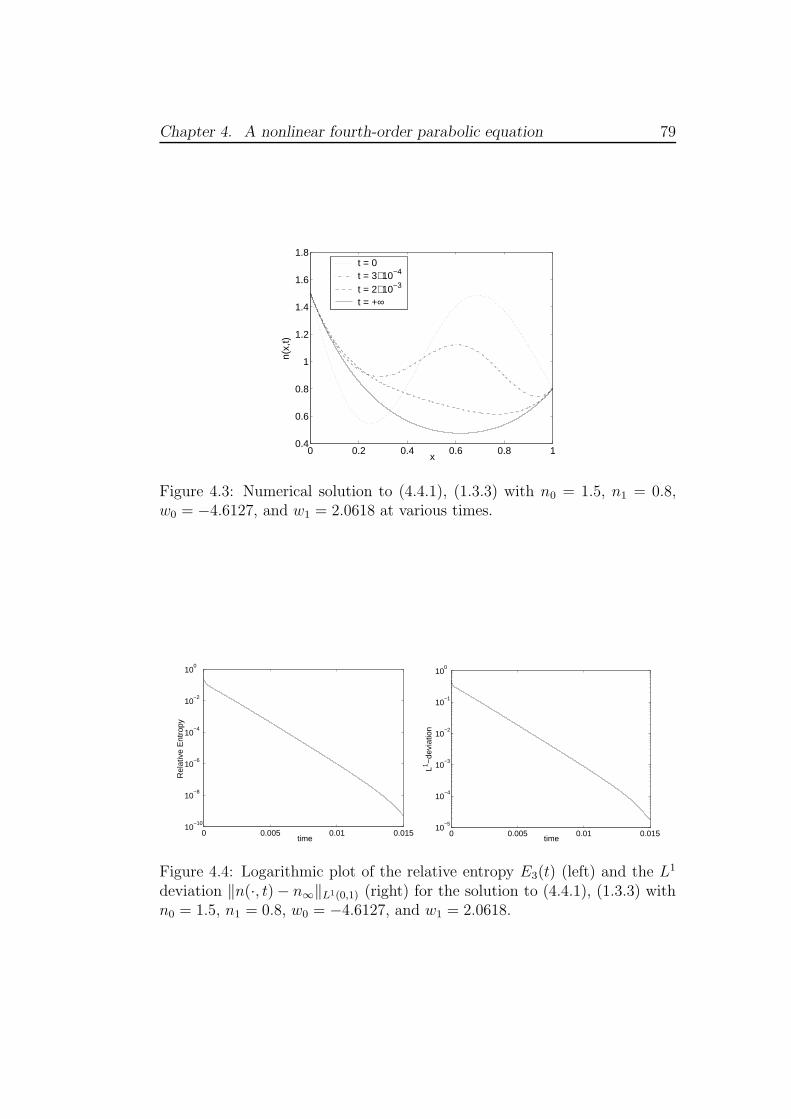
Chapter 4. A nonlinear fourth-order parabolic equation 79
0 0.2 0.4 0.6 0.8 10.4
0.6
0.8
1
1.2
1.4
1.6
1.8
x
n(x,
t)
t = 0t = 3⋅ 10−4
t = 2⋅ 10−3
t = +∞
Figure 4.3: Numerical solution to (4.4.1), (1.3.3) with n0 = 1.5, n1 = 0.8,w0 = −4.6127, and w1 = 2.0618 at various times.
0 0.005 0.01 0.01510
−10
10−8
10−6
10−4
10−2
100
time
Rel
ativ
e E
ntro
py
0 0.005 0.01 0.01510
−5
10−4
10−3
10−2
10−1
100
time
L1 −de
viat
ion
Figure 4.4: Logarithmic plot of the relative entropy E3(t) (left) and the L1
deviation ‖n(·, t) − n∞‖L1(0,1) (right) for the solution to (4.4.1), (1.3.3) withn0 = 1.5, n1 = 0.8, w0 = −4.6127, and w1 = 2.0618.
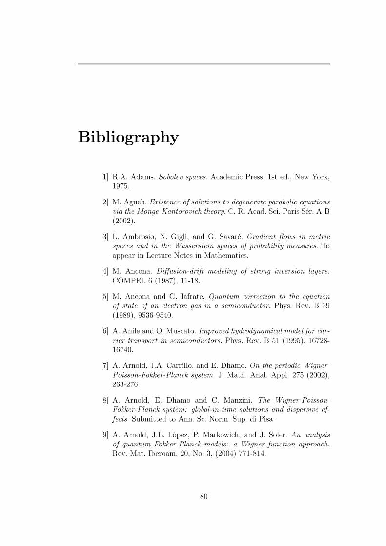
Bibliography
[1] R.A. Adams. Sobolev spaces. Academic Press, 1st ed., New York,1975.
[2] M. Agueh. Existence of solutions to degenerate parabolic equationsvia the Monge-Kantorovich theory. C. R. Acad. Sci. Paris Ser. A-B(2002).
[3] L. Ambrosio, N. Gigli, and G. Savare. Gradient flows in metricspaces and in the Wasserstein spaces of probability measures. Toappear in Lecture Notes in Mathematics.
[4] M. Ancona. Diffusion-drift modeling of strong inversion layers.COMPEL 6 (1987), 11-18.
[5] M. Ancona and G. Iafrate. Quantum correction to the equationof state of an electron gas in a semiconductor. Phys. Rev. B 39(1989), 9536-9540.
[6] A. Anile and O. Muscato. Improved hydrodynamical model for car-rier transport in semiconductors. Phys. Rev. B 51 (1995), 16728-16740.
[7] A. Arnold, J.A. Carrillo, and E. Dhamo. On the periodic Wigner-Poisson-Fokker-Planck system. J. Math. Anal. Appl. 275 (2002),263-276.
[8] A. Arnold, E. Dhamo and C. Manzini. The Wigner-Poisson-Fokker-Planck system: global-in-time solutions and dispersive ef-fects. Submitted to Ann. Sc. Norm. Sup. di Pisa.
[9] A. Arnold, J.L. Lopez, P. Markowich, and J. Soler. An analysisof quantum Fokker-Planck models: a Wigner function approach.Rev. Mat. Iberoam. 20, No. 3, (2004) 771-814.
80

Bibliography 81
[10] A. Arnold and A. Unterreiter. Entropy of discretized Fokker-Planckequations I - temporal semidiscretization. Comp. Math. Appl. 36(2003), 1683-1690.
[11] D. G. Aronson and P. Benilan. Regularite des solutions del’equation des milieux poreux dans RN . C. R. Acad. Sci. ParisSer. A-B 288 (1979), no. 2, A103–A105.
[12] C. Bardos, F. Golse, and C. Levermore. Fluid dynamic limits ofkinetic equation I: formal derivation. J. Stat. Phys. 63 (1991) 323-344.
[13] C. Bardos, F. Golse, and C. Levermore. Fluid dynamic limits ofkinetic equation I: convergence proofs for the Boltzmann equation.Comm. Pure appl. Math. 46 (1993), 667-753.
[14] J. Bebernes and D. Eberly. Mathematical Problems from Combus-tion Theory. Springer, Germany, 1989.
[15] N. Ben Abdallah and A. Unterreiter. On the stationary quantumdrift-diffusion model. Z. Angew. Math. Physik 49 (1998), 251-275.
[16] M. Bertsch, R. Dal Passo, G. Garcke, and G. Grun. The thinviscous flow equation in higher space dimensions. Adv. Diff. Eqs.3 (1998), 417-440.
[17] P. Bleher, J. Lebowitz, and E. Speer. Existence and positivity of so-lutions of a fourth-order nonlinear PDE describing interface fluc-tuations. Commun. Pure Appl. Math. 47 (1994), 923-942.
[18] F. Brezzi, I. Gasser, P. Markowich, and C. Schmeiser. Thermalequilibrium states of the quantum hydrodynamic model for semi-conductors in one dimension. Appl. Math. Lett. 8 (1995), 47-52.
[19] M. Caceres, J. Carrillo, and G. Toscani. Long-time behavior for anonlinear fourth order parabolic equation. TAMS 357 (2005) 1161-1175.
[20] A. O. Caldeira and A. J. Leggett. Path integral approach to quan-tum Brownian motion. Physica A, 121:587-616, 1983.
[21] J. A. Carrillo, M. Di Francesco and M. P. Gualdani. Semidis-cretization and long-time asymptotics of nonlinear diffusion equa-tions. Submitted for publication, 36 p., 2004.
Bibliography 82
[22] J.A. Carrillo, J. Dolbeault, P. Markowich and C. Sparber. Onthe long time behavior of the quantum Fokker-Planck equation.Monatsh. f. Math. 141 (2004), no. 3, 237 - 257.
[23] J.A. Carrillo, M.P. Gualdani and G. Toscani. Finite speed of prop-agation in porous media by mass transportation methods. C. R.Acad. Sci. Paris, Ser. I 338 (2004) 815-818.
[24] J.A. Carrillo, A. Jungel and S. Tang. Positive entropic schemes fora nonlinear fourth-order equation. Discrete Contin. Dynam. Sys.B 3 (2003), 1-20.
[25] J. A. Carrillo, A. Jungel, P. A. Markowich, G. Toscani and A.Unterreiter. Entropy dissipation Methods for degenerate ParabolicProblems and Generalized Inequality. Monatsh. Math. 133, 1-82(2001)
[26] J.A. Carrillo, R.J. McCann, and C. Villani. Contractions in the2-wasserstein length space and thermalization of granular media.Hyke preprint (www.hyke.org) (2004).
[27] J.A. Carrillo and G. Toscani. Asymptotic L1-decay of solutions ofthe porous medium equation to self-similarity. Indiana Univ. Math.J., 49, (2000), 113-142.
[28] J.A. Carrillo and G. Toscani. Wasserstein metric and large-time asymptotics of nonlinear diffusion equation. Hyke preprint(www.hyke.org) (2003).
[29] G. Chavent and J. Jaffre. Mathematical Models and Finite Ele-ments for Reservoir Simulation. Studies in Mathematics and itsapplications. North Holland, Amsterdam (1986).
[30] S.-K. Chua and R. Wheeden. Sharp conditions for weighted 1-dimensional Poincare inequalities. Indiana Univ. Math. J. 49(2000), 143-175.
[31] P. Degond, F. Mehats, and C. Ringhofer. Quantum hydrodynamicmodels derived from the entropy principle. To appear in Contemp.Math. (2005).
[32] P. Degond, F. Mehats, and C. Ringhofer. Quantum energy-transport and drift-diffusion models. J. Stat. Phys. 118 (2005) 625-665.
Bibliography 83
[33] P. Degond and C. Ringhofer. Quantum moment hydrodynamicsand the entropy principle. J. Stat. Phys. 112(3) (2003) 587-628.
[34] B. Derrida, J. Lebowitz, E. Speer, and H. Spohn. Fluctuations ofa stationary nonequilibrium interface. Phys. Rev. Lett. 67 (1991),165-168.
[35] L. Diosi. On high-temperature Markovian equation for quantumBrownian motion. Europhys. Lett. 22 (1993), 1-3.
[36] J. Dolbeault and M. del Pino. Best constants for Gagliardo-Nirenberg inequalities and applications to nonlinear diffusions. J.Math. Pures Appl. 81, (2002), 847–875.
[37] J. Dolbeault, I. Gentil, and A. Jungel. A nonlinear fourth-orderparabolic equation and related logarithmic Sobolev inequalities.Preprint, Universitat Mainz, Germany, 2004.
[38] H. Fujita. On the nonlinear equation ∆u+eu = 0 and ∂u∂t
= ∆u+eu.Bull. Amer. Math. Soc. 75 (1969), 132-135.
[39] I. Gamba and A. Jungel. Positive solutions of singular equationsof second and third order for quantum fluids. Arch. Rat. Mech.Anal. 156 (2001), 183-203.
[40] C. Gardner. The quantum hydrodynamic model for the semicon-ductor devices. SIAM J. Appl. Math. 54, 409-427, 1994.
[41] U. Gianazza, G. Savare, and G. Toscani. A fourth-order nonlinearPDE as gradient flow of the Fisher information in Wassersteinspaces. Preprint, Universita di Pavia, Italy, 2005.
[42] D. Gilbarg and N.S. Trudinger. Elliptic partial differential equa-tions of second order. 1st ed., Springer-Verlag, Berlin, 1983.
[43] H. Grubin and J. Kreskovsky. Quantum moment balance equationsand resonant tunneling structures. Solid-State Electr. 32 (1989),1071-1075.
[44] M. T. Gyi and A. Jungel. A quantum regularization of the one-dimensional hydrodynamic model for semiconductors. Adv. Diff.Eqs. 5 (2000), 773-800.
[45] M. P. Gualdani and A. Jungel. Analysis of the viscous quantum hy-drodynamic equations for semiconductors. Europ. J. Appl. Math.,(2004) vol. 15, 577-595.

Bibliography 84
[46] M.P. Gualdani, A. Jungel and G. Toscani. A nonlinear fourth-order parabolic equation with non-homogeneous boundary condi-tions. To appear in SIAM, J. Math. Anal. (2005).
[47] M.P. Gualdani, A. Jungel and G. Toscani. Exponential decay intime of solutions of the viscous quantum hydrodynamic equations.Appl. Math. Lett. 16 (2003), 1273-1278.
[48] A. Jungel. Numerical approximation of a drift-diffusion model forsemiconductors with nonlinear diffusion. ZAMM, Vol. 75 (1995),783-799.
[49] A. Jungel. A steady-state potential flow Euler-Poisson system forcharged quantum fluids. Comm. Math. Phys. 194 (1998), 463-479.
[50] A. Jungel. Quasi-hydrodynamic semiconductor equations.Birkhauser, Basel, 2001.
[51] A. Jungel and D. Matthes. A derivation of the isothermal quantumhydrodynamic equations using entropy minimization. To appear inZAMM, (2005).
[52] A. Jungel and Josipa-Pina Milisic. Macroscopic quantum modelswith and without collisions. Submitted for publication, 27 p., 2005.
[53] A. Jungel and R. Pinnau. A positivity preserving numerical schemefor a nonlinear fourth-order parabolic equation. SIAM J. Num.Anal. 39 (2001), 385-406.
[54] A. Jungel and R. Pinnau. Global non-negative solutions of a non-linear fourth-oder parabolic equation for quantum systems. SIAMJ. Math. Anal. 32 (2000), 760-777.
[55] A. Jungel and S. Tang. Numerical approximation of the viscousquantum hydrodynamic model for semiconductors. To appear inAppl. Numer. Math. (2005).
[56] A. Jungel and G. Toscani. Exponential Time Decay to a nonlinearfourth-order parabolic Equation. Z. Angew. Math. Phys. 54 (2003),377-386.
[57] A.S. Kalashnikov. Some problems of the qualitative theory ofsecond-order nonlinear degenerate parabolic equations. RussianMath. Surveys 42 (1987), no. 2(254), 169-222.
[58] B.F. Knerr. The porous medium equation in one space dimension.Trans. Amer. Math. Soc. 234 (1997), no. 2, 171-183.
Bibliography 85
[59] C. Levermore. Moment closure hierarchies for kinetic theories. J.Stat. Phys. 83 (1996) 1021-1065.
[60] C. Levermore. Entropy-based moment closures for kinetic equa-tions. Trans. Theory Stat. Phys. 26 (1997) 591-606.
[61] M. Loffedro and L. Morato. On the creation of quantum vortexlines in rotating HeII. Il nuovo cimento 108B (1993), 205-215.
[62] E. Madelung. Quantentheorie in hydrodynamischer Form. Z.Physik, 40:322, 1927.
[63] P.A. Markowich. The stationary semiconductor device equations.Springer-Verlag, Vienna, New York, 1986.
[64] P.A. Markowich, C. Ringhofer, and C. Schmeiser. SemiconductorEquations. Springer-Verlag, Vienna, New York, 1990.
[65] P.A. Markowich, C. Villani. On the trend to equilibrium for theFokker-Planck equation: an interplay between physics and func-tional analysis, Proceedings, VI Workshop on Partial Differen-tial Equations, Part II (Rio de Janeiro, 1999). Mat. Contemp. 19(2000), 1–29.
[66] F. Otto. The geometry of dissipative evolution equations: theporous medium equation, Comm. Partial Differential Equations 26(2001) 101-174.
[67] R. Pinnau. A note on boundary conditions for quantum hydrody-namic equations. Appl. Math. Lett. 12 (1999), 77-82.
[68] R. Pinnau and A. Unterreiter. The stationary current-Voltagecharacteristics of the quantum drift diffusion model. SIAM J. Num.Anal., 37(1), 211-245 (1999).
[69] F. Poupaud. Etude mathematique et simulation numerique dequelques equations de Boltzmann. Phd thesis, Universite de Nice,France, 1988.
[70] J. Simon. Compact sets in the space Lp(0, T ;B). Ann. Mat. PuraAppl., IV. Ser. 146 (1987), 65-96.
[71] M. Taylor. Pseudodifferential Operators. Princeton UniversityPress, Princeton, 1981.

Bibliography 86
[72] A. Unterreiter. The thermal equilibrium solution of a generic bipo-lar quantum hydrodynamic model. Comm. Math. Phys., 188, 69-88,(1997).
[73] W. Van Roosbroeck. Theory of flow of electron and holes in ger-manium and other semiconductors. Bell Syst. Techn. J. 29 (1950),560-607.
[74] J. L. Vazquez. Asymptotic behaviour and propagation properties ofthe one-dimensional flow of gas in a porous medium. Trans. Amer.Math. Soc. 277 (1983), no. 2, 507-527.
[75] J. L. Vazquez. An introduction to the mathematical theory of theporous medium equation. Shape optimization and free boundaries(Montreal, PQ, 1990), NATO Adv. Sci. Inst. Ser. C Math. Phys.Sci., vol. 380, Kluwer Acad. Publ., Dordrecht, 1992, pp. 347-389.
[76] J. L. Vazquez. Asymptotic behaviour for the porous medium equa-tion posed in the whole space. J. Evol. Equ. 3 (2003), 67-118.
[77] C. Villani. Topics in optimal mass transportation. Graduate stud-ies in Mathematics, vol. 58, American Mathematical Society, Prov-idence, RI (2003).
[78] A. Wettstein. Quantum effects in MOS devices. Volume 94 of Seriesin Microelectronics, Hartung-Gorre, Konstanz, 2000.
[79] E. Wigner. On the quantum correction for thermodynamic equilib-rium. Phys. Rev. 40 (1932), 749-759.
[80] E. Zeidler. Nonlinear functional analysis and its applications. 1sted., Springer-Verlag, Berlin, 1990.
[81] B. Zhang and J. Jerome. On a steady-state quantum hydrodynamicmodel for semiconductors. Nonlin. Anal. 26 (1996), 845-856.
[82] J. Zhou and D. Ferry. Simulation of ultra-small GaAs MESFETusing quantum moment equations. IEEE Trans. Electr. Devices 39(1992), 473-478.