1

Abstract— The main objective of this work was to analyse real

network data, for both UMTS and LTE, and to fit statistical distributions that enable the identification of worst sites within a network, regarding two parameters: delay variation and packet loss. Both parameters were measured in the link between the network site and its controller, which can be a microwave or an optical fibre one. Possible sources for both these problems are also discussed along this work. The fitting of a statistical distribution to every site, best representing the behaviour of each parameter, is an effort to predict their behaviour throughout time. For this, a program in MATLAB© was developed, that contains an algorithm to process and evaluate data samples; in its core, it is a Chi-Square goodness-of-fit test, to ascertain which distribution better fits the investigated parameters from a pre-defined group of distributions. For the used scenario, it is concluded that one can model, with a significance level of 95%, 60% of the UMTS NodeB’s delay variation via the Generalised Extreme Value distribution, while regarding packet loss, 56% can be model through the Log-logistic one. As for LTE, the Weibull and the Generalised Extreme Value distributions describe best the behaviour of the same parameters, for 75% of all the sites analysed for both cases. It is also found that link capacity and traffic volume are the aspects that have more influence in the parameters studied.

Index Terms—Delay Variation, Goodness-of-Fit, LTE, Packet Loss, Statistical Distributions, UMTS.

I. INTRODUCTION OBILE communications have become an everyday commodity. In the last couple of decades, they have

changed from being an expensive technology only reserved for a few, to being one of the most used services worldwide. The rapid development of the technology used in telecommunication systems, consumer electronics, and mobile devices, has been remarkable in the past 20 years. The continuing evolution of processor performance, as predicted by Moore’s law, along with cheaper methods of fabrication and large-scale economies, resulted in very low-cost equipment available to everyone, spreading the mobile phone everywhere in the world. With it, a new multitude of mobile devices appears, with electronic tablets, laptops and a whole

P. A. Venâncio, M.Sc. Student, Instituto Superior Técnico (IST), Lisbon,

Portugal (e-mail: pvenancio76@gmail.com). L. M. Correia, Professor, Instituto Superiro Técnico (IST) – INOV/INESC,

Univertisty of Lisbon, Lisbon, Portugal (e-mail: luis.correia@inov.pt). C. Bedini, Engineer, Ericsson Portugal, Lisbon, Portugal (e-mail:

chiara.bedini@ericsson.com).

new range of “smarter” phones being the front-runners of this evolution, where data connections surpass voice ones. It is expected that by the end of 2015 there will be over 10 billion of these devices around the world. Cellular systems standards have continually been evolving, where organisations like the 3rd Generation Partnership Project (3GPP) helped directing this evolution towards the latest generation of cellular systems, LTE – Long Term Evolution [1].

Since LTE is still being deployed, the traffic load for the network is not very high at the moment. Due to the low number of current subscribers, performance assessment is not very clear, because many services are running in very favourable conditions. Sometimes performance can be assessed from the UMTS network, since both LTE and UMTS have some elements in common. From the user perspective, it is the end-to-end quality that needs to be classified, or in other terms, the Quality of Experience (QoE), that involves data rate and delay. On the operator side, other parameters need to be taken into account, like packet drop and delay variation. Since packet loss can result in highly noticeable performance issues, while for real-time applications delay variation stands out as the main problematic concern, both parameters are of the greatest importance inside the network. Thus, the goal of this work was to model these parameters through statistical distributions, and to predict their behaviours through time.

Although one can analyse packet loss and delay variation between two points anywhere inside the network, it is in the link between the NodeB or eNodeB and the RNC or MME, respectively, that packet loss and delay variation are most problematic. An identification of the problem source is also needed, aimed to help the operator tracing to where they are, so that they can take the proper steps to mitigate them.

This work is divided into five parts. Part II describes how the performance parameters being analysed are measured, Part III elaborates on the models developed for measuring the parameters and Part IV presents their results. Part V is accountable for the conclusions of the work made here.

II. PERFORMANCE PARAMETERS Nowadays packet delay can be easily calculated through the

difference between the transmission instant of a packet, in the transmitting node of the network, and the receiving time of that same packet in the receiving node: 𝛥𝑇 !!  = 𝑡!"# − 𝑡!"#$% (1)

where 𝛥𝑇 is the delay measured, 𝑡!"# is the receiving time of

Analysis of Network Quality Using Non-Intrusive Methods from an End-User Perspective in LTE

Pedro A. Venâncio, Luís M. Correia, and Chiara Bedini

M

2

the packet, and 𝑡!"#$% is the transmitting time of that same packet. Consequently, delay variation, is simply the difference between two consecutive packet delay measurements: 𝛿 !! = |𝛥𝑇! − 𝛥𝑇!!!| (2)

where 𝛿 is the packet delay variation, and 𝛥𝑇! is the time delay of packet 𝑖. However different methodologies can be applied. In [2], a measurement that is a hybrid between active probing and passive monitoring is used, where probe packets are injected into the network. In [3], the authors used QoSMeT tool, that sniffs both the departing and arriving packets directly from the network interface device, where in [4] the authors elaborate on the influence of packet size on the delay, using passive measurement that will not affect any part of the network. In this work, it is used the method calculated by (2).

As for packet loss, the preeminent parameter being of any given packet network, it is possible to measure it in two different ways, achieving mostly the same results. One way is measure it from the point of view of the transmitter:

𝐿! % = 100𝑁!"#"$%

𝑁!"#"$% + 𝑁!"#$ (3)

where 𝐿! is the packet loss from the point of view of the transmitter, 𝑁!"#$ is the number of packets sent to the peer node, in a unit of time, and 𝑁!"#"$% is the number of packets resent to the peer node in the same unit of time. The other way of measuring packet loss is through the perspective of the receiver network node, which is calculated from:

𝐿! % = 100𝑁!

𝑁! + 𝑁! (4)

where 𝐿! is the packet loss from the point of view of the receiver, 𝑁! is the number of packets received by the node, in a unit of time, and 𝑁! is the number of packets that were not correctly received by the node, or lost, in the same unit of time, due to, e.g., wrong decoding or destroyed frames.

III. MODELS

A. Statistical Distributions In order to evaluate the performance of a site, one has to

analyse the data originated from it. On the other hand, if a prediction has to be made, based on the collected and analysed data, on whether the same site will have performance problems in the future, regarding delay variation or packet loss, a statistical model has to be developed to estimate the evolution of the concerned performance parameters associated to the base station. One can accomplish this by finding the best statistical distribution that fits the evaluated data, sharing its properties in terms of behaviour over time, average value and standard deviation, which are all characteristic, and sometimes similar, for each distribution.

Of all statistical distributions available, a small group was taken into account upon the development of the model that is used in this work: Gamma, Generalised Extreme Value (GEV), Inverse Gaussian (IG), Logistic, Log-logistic, Log-normal, Nakagami, Rayleigh, Rice, and Weibull. This collection was elaborate considering the nature of the parameters to analyse, where the principal factor was that both

packet loss and delay variation are positive variables. The choice of the distributions had this in account: some of the considered distributions have the random variable within ]0,  +∞[, while others, although having the random variable ranging in ] −∞, +∞[, are capable of having its range bounded and be defined only for positive values. Another characteristic is the shape of the PDF [5]; it is expected that the PDF has a non-symmetric bell-shaped evolution, similar to a Normal distribution (not in the symmetric aspect), so there are some distributions that one can exclude a priori, like the Uniform and Exponential distributions, where their PDFs are constant or strictly increasing over its range, respectively.

B. Goodness-of-fit When assuming that data follows a specific distribution, if

the assumed distribution does not hold then the confidence levels of the hypothesis tests implemented may be completely off. One way to deal with this problem is to check distribution assumptions carefully, so that a precise and correct model can be developed for the problem in question.

There are two approaches to checking distributions assumptions. One is via empirical procedures, mainly through graphic interpretation. They are easy to understand and to implement, and are based on intuitive and graphical properties of the distribution that one wants to assess. The other is via Goodness-of-Fit (GoF) tests. Based on statistical theory, the GoF tests are formal procedures, that usually require specific numerical computing software to aid through their lengthy and heavy calculations, but their results are quantifiable and more reliable than the ones obtained from the empirical procedures. One of these tests, among the different available, and the one used in this work, is the Chi-Squared GoF test.

The Chi-Squared GoF test is applied to binned data (i.e., data put into classes). So, to perform the test, first one has to select convenient values of the data range that divide it accordingly into several subintervals, which do not necessarily have to have the same size, but need to be equal or more than 5, due to the lower limit of the Degree of Freedom (DF), as explained further ahead in this subsection. Then, the number of data points in each subinterval has to be evaluated. These are called “observed” values, and the Chi-Square test requires at least 5 of them in every subinterval. If there are less than 5 samples in each one, the subintervals need to be increased to accommodate more samples, by merging it with the adjacent subintervals, or, in a limit case where is not possible to merge with any other else because of the minimum limit of 5 subintervals, this defective subinterval is excluded. Note that the result of the test is not affected if the subintervals that cannot be merged are eliminated, since they do not represent the majority of the whole data but only an insignificant part of it, thus not compromising the test. A detailed version on how to assess data with the Chi-Square GoF one can see [6].

Another process to evaluate the distribution fitting, even if it is only to have a first guess of the distribution fitted to the data and to outwit some initial cases from the process, is by measuring the correlation and the Mean Square Error (MSE) between the PDF of the hypothetical distribution and the histogram of the actual data. Correlation 𝑐𝑜𝑟𝑟, obtained by (5) [7], is the dependence between two variables 𝑋 and 𝑌, where a

3

result of 1 means total correlation and 0 represents no correlation between the variables.

𝑐𝑜𝑟𝑟 =𝑥! − 𝑥 𝑦! −  𝑦!

!!!

𝑥! − 𝑥 !!!!! 𝑦! − 𝑦 !!

!!!

(5)

where 𝑐𝑜𝑟𝑟 is the correlation value, 𝑥! and 𝑦! are the variables to correlate, 𝑥 and 𝑦 are the average of the variable to correlate, and 𝑁 is the number of samples of each variable. As for MSE, it measures the average of the squares of the errors, that is, the difference between the estimator and the estimated, i.e., the PDF of the hypothetical distribution and the histogram of the evaluated data, respectively. It is calculated by:

𝜀! =1𝑁

𝑌! − 𝑌!!

!

!!!

(6)

where 𝜀! is the MSE, 𝑌! is the estimated value for the PDF at the center of the histogram cell 𝑖, 𝑌! is the histogram cell value 𝑖, and 𝑁 is the number of samples of each variable.

C. Data Analysis Model In order to evaluate the data, a program was developed in

MATLAB© to aid in the processing and calculations required by the methods that have been chosen to use.

Regarding the main program, first one has to create the basic structures to store the data and define the default program parameters values. The thresholds, which will add an upper limit to the sample values, so that the occasional data peaks and anomalies do not disrupt the tests, are also defined, as long as the minimum amount of data samples that a site must have, so that a statistical relevant analysis can be done. Afterwards, it is needed to import, individually, the data related to the network parameters to be analysed (delay variation or packet loss), and store it in appropriate data structures. These steps were labelled DEFAULTS and IMPORT, respectively, being depicted in Fig. 1.

The next step consists of searching for data peaks in the imported samples. In PEAK ANALYSIS, each sample is compared with the previously mentioned threshold, which limits the maximum value these samples can take. If the sample value is lower than the threshold, then the sample is saved, otherwise the sample is removed. The number of data peaks each of the considered sites has is stored in memory, so that an analysis can be done on top of that information.

The core process of the program is DATA ANALYSIS. For each site, first, it is needed to verify that there is a minimum amount of samples to work with, from the ones left from PEAK ANALYSIS, so that a reliable statistical result can be obtain with the GoF tests. If it is found that there is a lack of data samples, the site is considered improper to be analysed, and another site has to be chosen. Subsequently, after defining the distributions that are going to be evaluated when fitting the data, the Chi-Square GoF test is performed for each one, with a significance level φ = 95%, and the correlation and MSE between the distribution PDF and the histogram of the imported data is calculated. Due to the fact that one of the objectives of this model is to represent all sites with one, or more if it not possible with one, distribution, then after the DATA ANALYSIS block, an OPTIMISATION process is made, in order to reassign a distribution to a site based on the

results from the previous block. All the results of the three computations are taken into account to identify the best distribution that represents the site.

Fig. 1. Structural diagram of the data analysis model developed in MATLAB©.

Afterwards, the topology of the network where these sites belong is inserted (in TOPOLOGY ANALYSIS), so that one can try to correlate the number of hops, or jumps from one node of the network to the next one, with the resulting distributions adjusted and their core parameters.

The latitude and longitude information of the sites is also imported in GEOGRAPHIC ANALYSIS, so that one can have a higher view of the network and the overall performance state of it, since problematic sites are market as such.

In the end of the program, the various distribution results are exported and saved to an external file, in the SAVE block.

Note that, along the deployment of the program, one is able to extract multiple graphical plots regarding any kind of process block, for an easy and constantly monitoring of the evolution of the program, and to assess the results obtained during and at the end of the analysis process.

4

D. Network Link Model To investigate possible problem sources for packet loss and

delay variation, a model of the network link between the base station and the RNC or MME, for both optical and microwave instances, was also developed.

A one-way connection is considered for the optical link, since a bidirectional link has a similar scheme. The model corresponds to the usual optical connection [8]. For the transmitter, it is considered as a simple electric-optical information converter, being then connected to the fibre. All the main factors that induce power loss in the link are also presented: connectors and splices. In terms of optical amplification, two mainly used approaches are considered: one with a regenerator, and the other with an optical amplifier. At the end of the link it is possible to find an also simple photo detector receiver. The average optical power that reaches the receiver is directly connected to the percentage of packets lost in the link, in the sense that a lower received power needs a more sensitive receiver to guarantee the same levels of performance. If the power received drops below the minimum required to sustain a certain degree of performance, the receiver is not able to differentiate the actual signal from communication noise, leading to the packet being dropped.

The microwave link model, likewise the previous one, can also be depicted as an aggregation of different major blocks [9]. The baseband data traffic, overhead bytes for signalling, service channels, and radio control are fed into a multiplexer, where they are combined into an aggregate digital stream, which is done in the MULDEM (Multiplexer-Demultiplexer) block. Afterwards, this aggregated stream is condensed into a more efficient bit stream with a reduced bandwidth in the modulator, the MODEM (Modulator-Demodulator) block. A conversion to an Intermediate Frequency (IF), where amplification is easier in terms of linearity, and then up converted to Radio Frequency (RF) and fed to the high power amplifier module in the final stage, is done in the TRANS-RECEIVER. This signal is then fed to the branching unit for connection to the antenna to be transmitted.

In the receiver, the baseband signal is recovered by the demodulator, which, after, detects and decides, converts the signal in a sequence of bits. Once the sequence of bits transmitted is reconstructed, one has to identify the signal within it. Is in this process that the power received affects the packet loss of the inferred link. Like in the optical part, if the signal power received is low, the noise will overcome the signal, and thus a coherent detection of the bits is not possible, leading to misconceived frames, that ultimately are discarded, helping increase the percentage of packets lost within the link.

IV. RESULTS ANALYSIS

A. Scenario The scenario used for this work consists of a part of an

access network of UMTS and LTE, installed in a major city. For UMTS, it is only considered the sites that are connected to one specific RNC, as for LTE it was possible to consider all of its sites, all connected to a single MME. Both the RNC and the MME share the same physical location in the city. With also, all eNBs being collocated with NodeBs, thus sharing the same links to reach the respective MME or RNC. Were considered

110 NodeBs and 36 eNBs. As stated before, the NodeBs and eNBs can be connected to the RNC or MME in two different ways: through optical fiber, or by one or more microwave links and then optical fiber. When a site is connected to the RNC or MME only by fiber, it is designated that it does not have any hop, or jump. When a site has to pass through one, or two, microwave links to reach its destination, it is designated that it has one, or two, hops.

TABLE I NUMBER OF SITES WITH SPECIFIC NUMBER OF HOPS

Number of Hops Network 0 1 2 UMTS 31 54 25 LTE 14 15 7

The data from these sites were obtained through ESAT

(Ericsson Stats Analysis Tool), a software that manages the entire network, and, consequently, all the sites under analysis. Due to confidentiality issues, each site will be identified by its corresponding SiteID. For comparison purposes, one has chosen two ranges of days associated to two different scenarios: weekdays (3 to 7 of February, 2014) and weekends (8 and 9 of February, 2014), with a time granularity of 15 minutes was used, since it is the smallest one that tool enables. Table II shows how many samples were analysed for each network, and for each type of days.

TABLE II NUMBER OF SAMPLES FOR EACH PARAMETER FOR ALL SCENARIOS ANALYSED

UMTS LTE Parameter Weekdays Weekend Weekdays Weekend

Delay Variation 50 801 20 214 17 329 6 753 Packet Loss 50 803 20 926 17 217 6 909

Finally, one has defined another group of values to be use in the model: the thresholds. In order to be considered to have a good performance within each parameter, each site must have its average value below the thresholds of 20 µs and 1%, for delay variation and packet loss, respectively. These values were provided by Ericsson, as the standard values for both parameters threshold performance. Regarding the minimum amount of required samples, each site needs a minimum of 80 samples to be eligible for evaluation, because a lower value wouldn’t provide a reasonable statistical approximation. For the peak status of each sample, a peak of delay variation sample is considered if it surpasses the value of 100 µs, and a peak of packet loss data appears when a sample is greater than the threshold value of 15% of packets lost per unit of time. Both values were obtained by observing the performance thresholds that are considered. Since those are the values to achieve, the peak thresholds chosen are high enough so that any sample that reaches them can be safely labelled as a peak.

B. UMTS Data Analysis In this section, one shows the results obtained for UMTS,

through the Data Analysis Model developed. First the results for Delay Variation and Packet Loss are presented, while after an overview of the overall UMTS scenario is given. 1) Delay Variation

The results of the model used can be divided into several parts. The first results come from the analysis of data peaks: one has found 323 delay variation peaks in weekdays, resulting in 0.64% of samples above the threshold for peak

5

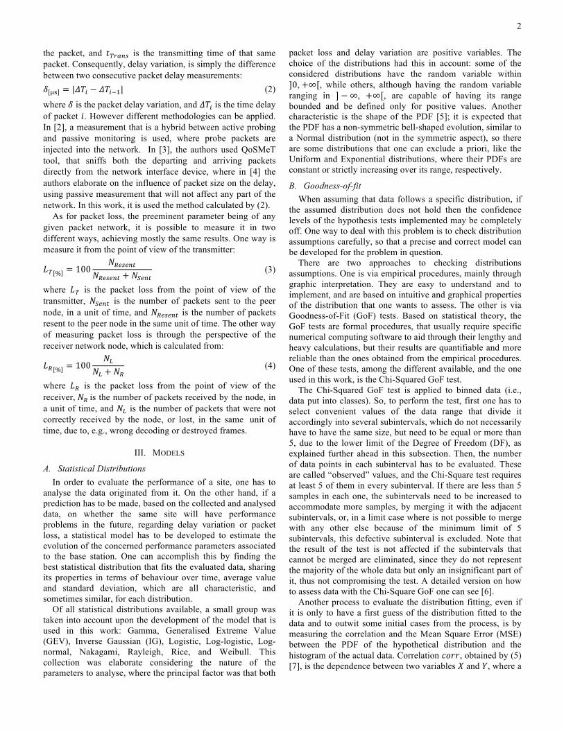
status, and 106 peaks in the weekend, resulting in 0.52% of peaks, thus concluding that, even though there are more peaks during weekday, the proportion of peaks does not change, hence, the number of peaks does not depend on the specific day. Regarding the analysis of the NodeBs, cleaned of data peaks, it was verified that 44 did not had sufficient delay variation data to be properly processed, meaning that only 60% of both UMTS scenarios (weekdays and weekends) were evaluated. Among them, SiteID_8 stands out as the worst site for both scenarios, regarding delay variation, with an average sample value close to 48 µs, as can be seen in Fig. 2.

Fig. 2. SiteID_8 delay variation samples over weekdays (top) and on the weekend (bottom).

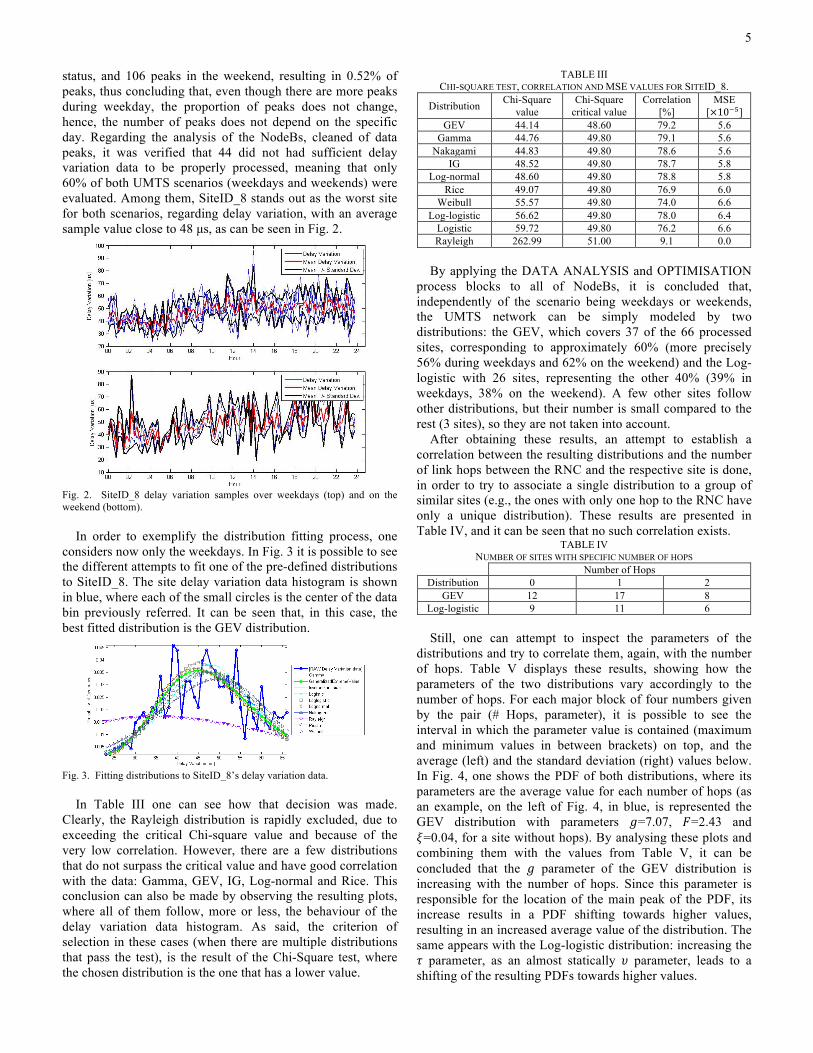
In order to exemplify the distribution fitting process, one considers now only the weekdays. In Fig. 3 it is possible to see the different attempts to fit one of the pre-defined distributions to SiteID_8. The site delay variation data histogram is shown in blue, where each of the small circles is the center of the data bin previously referred. It can be seen that, in this case, the best fitted distribution is the GEV distribution.

Fig. 3. Fitting distributions to SiteID_8’s delay variation data.

In Table III one can see how that decision was made. Clearly, the Rayleigh distribution is rapidly excluded, due to exceeding the critical Chi-square value and because of the very low correlation. However, there are a few distributions that do not surpass the critical value and have good correlation with the data: Gamma, GEV, IG, Log-normal and Rice. This conclusion can also be made by observing the resulting plots, where all of them follow, more or less, the behaviour of the delay variation data histogram. As said, the criterion of selection in these cases (when there are multiple distributions that pass the test), is the result of the Chi-Square test, where the chosen distribution is the one that has a lower value.

TABLE III CHI-SQUARE TEST, CORRELATION AND MSE VALUES FOR SITEID_8.

Distribution Chi-Square value

Chi-Square critical value

Correlation [%]

MSE [×10!!]

GEV 44.14 48.60 79.2 5.6 Gamma 44.76 49.80 79.1 5.6

Nakagami 44.83 49.80 78.6 5.6 IG 48.52 49.80 78.7 5.8

Log-normal 48.60 49.80 78.8 5.8 Rice 49.07 49.80 76.9 6.0

Weibull 55.57 49.80 74.0 6.6 Log-logistic 56.62 49.80 78.0 6.4

Logistic 59.72 49.80 76.2 6.6 Rayleigh 262.99 51.00 9.1 0.0

By applying the DATA ANALYSIS and OPTIMISATION

process blocks to all of NodeBs, it is concluded that, independently of the scenario being weekdays or weekends, the UMTS network can be simply modeled by two distributions: the GEV, which covers 37 of the 66 processed sites, corresponding to approximately 60% (more precisely 56% during weekdays and 62% on the weekend) and the Log-logistic with 26 sites, representing the other 40% (39% in weekdays, 38% on the weekend). A few other sites follow other distributions, but their number is small compared to the rest (3 sites), so they are not taken into account.

After obtaining these results, an attempt to establish a correlation between the resulting distributions and the number of link hops between the RNC and the respective site is done, in order to try to associate a single distribution to a group of similar sites (e.g., the ones with only one hop to the RNC have only a unique distribution). These results are presented in Table IV, and it can be seen that no such correlation exists.

TABLE IV NUMBER OF SITES WITH SPECIFIC NUMBER OF HOPS

Number of Hops Distribution 0 1 2

GEV 12 17 8 Log-logistic 9 11 6

Still, one can attempt to inspect the parameters of the

distributions and try to correlate them, again, with the number of hops. Table V displays these results, showing how the parameters of the two distributions vary accordingly to the number of hops. For each major block of four numbers given by the pair (# Hops, parameter), it is possible to see the interval in which the parameter value is contained (maximum and minimum values in between brackets) on top, and the average (left) and the standard deviation (right) values below. In Fig. 4, one shows the PDF of both distributions, where its parameters are the average value for each number of hops (as an example, on the left of Fig. 4, in blue, is represented the GEV distribution with parameters 𝑔=7.07, 𝐹=2.43 and 𝜉=0.04, for a site without hops). By analysing these plots and combining them with the values from Table V, it can be concluded that the 𝑔 parameter of the GEV distribution is increasing with the number of hops. Since this parameter is responsible for the location of the main peak of the PDF, its increase results in a PDF shifting towards higher values, resulting in an increased average value of the distribution. The same appears with the Log-logistic distribution: increasing the 𝜏 parameter, as an almost statically 𝜐 parameter, leads to a shifting of the resulting PDFs towards higher values.

6

TABLE V DISTRIBUTION PARAMETERS VS. NUMBER OF HOPS TO RNC.

Generalised Extreme Value Log-logistic # Hops 𝑔  (location) 𝐹 (scale) 𝜉 (shape) 𝜏 (scale) 𝜐 (shape)

0 [2.5, 14.0] [0.9, 5.0] [-0.2, 0.3] [0.9, 2.8] [0.1, 0.3] 7.0 4.4 2.4 1.6 0.1 0.2 1.5 0.7 0.2 0.1

1 [3.0, 43.4] [0.8, 10.4] [-0.2, 0.7] [1.1, 3.1] [0.2, 0.4] 12.3 12.7 3.8 2.8 0.1 0.3 1.9 0.7 0.2 0.1

2 [4.0, 32.9] [1.0, 7.5] [-0.4, 0.4] [1.4, 2.7] [0.1, 0.2] 13.5 10.4 3.9 2.3 -0.1 0.3 1.9 0.5 0.2 0.1

Fig. 4. Resulting distributions (left for GEV and right for Log-logistic) considering mean value of its parameters.

By analysing these results, it is possible to conclude that the

delay variation suffered by a NodeB is connected to the number of hops between it and the RNC: a higher number of hops leads to an increase of the average delay variation, independently of the distribution that represents the site. 2) Packet Loss

In terms of packet loss, the overall number of peaks is smaller: 23 in weekdays and 32 in the weekend, which are approximately 0.05% and 0.15% of all samples, respectively.

Observing Fig. 5, that represent the worst sites for the two scenarios, one can confirm the definitive factor that influences the behaviour of packet loss: volume of data traffic. The packet loss decreases during night hours, when the amount of users using the system is lower.

Fig. 5. Behaviour of the worst sites for the two scenarios: SiteID_25 during weekdays (top) and SiteID_82 during weekends (bottom).

Considering again the process of finding a distribution that can be used to model packet, the final results are showed, after the optimisation processes, in Table VI.

In this case, one has obtained two different pairs of distributions for each scenario. During weekdays, the sites can

be mainly represented by the Log-logistic and Nakagami distributions: a total of 55 sites, representing 56% of the 99 sites analysed, are represented by the Log-logistic distribution, and 31 sites, representing 31% of the same amount of sites, are represented by the Nakagami distribution. Again, a small amount of sites are represented by other distribution than these two, and are neglected. During the weekend, the Log-logistic distribution maintains itself as one of the best distribution to represent the sites data, with 41 sites (49% of the total 84 with enough data to be analysed), but the Nakagami is replaced by the Log-normal distribution, this one now representing 27 sites (32%), while other distributions represent the remaining 16.

TABLE VI REPRESENTATIVE DISTRIBUTIONS FOR PACKET LOSS IN UMTS.

Distribution Weekdays Weekend Log-logistic 55 41 Log-normal 0 27 Nakagami 31 5

Other 13 11 Continuing with the same analysis process, the resulting

distributions were investigated to assess if a correlation exists between them and the number of hops in the link between the site and the RNC. The results are in Table VII and Table VIII.

TABLE VII DISTRIBUTIONS VS. NUMBER OF HOPS - WEEKDAYS SCENARIO. Number of Hops

Distribution 0 1 2 Log-logistic 17 25 13 Nakagami 7 16 8

TABLE VIII

DISTRIBUTIONS VS. NUMBER OF HOPS - WEEKEND SCENARIO. Number of Hops

Distribution 0 1 2 Log-logistic 13 17 11 Log-normal 7 12 8

Similarly to delay variation, there is no obvious correlation

between the distributions and the amount of sites with a given number of hops. Still, the other test can be made, by analysing the distribution parameters and try to identify if a connection between them and the number of hops exists. Starting with the weekdays scenario, in Table IX the results are presented.

TABLE IX PACKET LOSS DISTRIBUTION PARAM. VS. NUM. OF HOPS TO RNC - WEEKDAYS.

Log-logistic Nakagami # Hops 𝜏 (shape) 𝜐 (scale) 𝑚 (shape) 𝛺 (spread)

0 [0.7, 1.7] [0.2, 0.6] [0.1, 0.7] [12.7, 588.2] 1.2 0.2 0.4 0.1 0.5 0.3 176.78 227.6

1 [-0.9, 2.4] [0.3, 2.5] [0.2, 1.8] [0.2, 2049.7] 1.0 0.6 0.6 0.2 0.4 0.4 434.0 638.4

2 [-0.3, 1.5] [0.2, 0.8] [0.2, 0.5] [13.1, 1290.6] 1.0 0.5 0.5 0.2 0.3 0.1 540.7 571.8

Focusing first on the Log-logistic, it is not possible to see a

constant evolution of the parameters. Although the average value of the shape parameter 𝜏 decreases with the number of hops, the scale parameter 𝜐 does not have a similar behaviour. By observing the plots in Fig. 6, that again result from imputing the average values obtained in the Log-logistic distribution parameters, one can conclude that these variations in the parameters do not affect strongly the overall variation of the distribution, with the average value of the distribution for

7

all cases being maintained around 3% and 4% of packet loss. Concerning the Nakagami distribution, the behaviour of the parameters is different: the 𝑚 parameter decreases with the number of hops, while the 𝛺 one increases. Observing the resulting graphic plots in Fig. 6, one can see that the average and standard deviation values of the distributions are higher than the ones for the Log-logistic case. Even though the change in shape, that has a large effect in the lower values of the distribution range (higher probability of lower packet loss percentage for the one and two hops case, contrarily to what happens for zero hops), the overall number of sites represented by the Nakagami distribution suffer from high average and standard deviation values, putting all of them into the bad performance group of sites.

Fig. 6. Resulting distributions (left for Log-logistic and right for Nakagami) considering mean value of its parameters – weekdays.

Focusing now on the weekend scenario, the results are in Table X. In terms of the Log-logistic distribution, the same as the previous scenario occurs, but this time it is the 𝜐 parameter that has a increasing behaviour with the number of hops, and the values of 𝜏 do not follow similar pace. Observing the plots in Fig. 7 it can be seen that they are very similar to the ones in Fig. 6, where the average value of the distributions continues to be around the 3% and 4% of packets lost, thus, the explanation done for the previous case is maintained here.

TABLE X PACKET LOSS DISTRIBUTION PARAM. VS. NUM. OF HOPS TO RNC - WEEKDAYS.

Log-logistic Log-normal # Hops 𝜏 (shape) 𝜐 (scale) 𝜂 (shape) 𝜙 (spread)

0 [0.1, 1.8] [0.3, 0.6] [0.8, 1.6] [0.7, 1.0] 1.3 0.5 0.4 0.1 0.8 0.3 0.9 0.1

1 [-0.9, 2.0] [0.3, 0.8] [-0.1, 1.6] [0.6, 1.2] 1.1 0.7 0.5 0.1 1.0 0.6 1.0 0.2

2 [0.1, 2.6] [0.4, 0.8] [-0.8, 1.5] [0.8, 1.8] 1.2 0.8 0.6 0.2 0.6 0.9 1.1 0.4

Fig. 7. Resulting distributions (left for Log-logistic and right for Log-normal) considering mean value of its parameters – weekend.

As for the Log-normal distribution, although the parameters being different from the ones of the Nakagami distribution, their behaviour is equal: 𝜂 decreases and 𝛺 increases. These results are presented in Fig. 7, where one can see that the peak

of packet loss probability is shifted closer to the origin as the number of hops increases, suggesting that some mechanism exists in these group of sites links that disable the loss of packets when they jump from one link to the other. It also can be seen that the average value of the packet loss in these sites has values around 2% and 3%.

With these results, one can conclude that the sites modelled by the Log-logistic distributions are not affected by the different number of hops they may have. Still, the ones modelled by the Nakagami distribution have higher standard deviation values, independently of the number of hops, while the Log-normal ones present a decreasing in the average value of the distribution when the number of hops increases. 3) UMTS Overview

An overview on the results of the two previous subsections is done, so that one can conclude if this network has an overall good of bad performance. Table XI represents the status of the complete network in terms of packet loss and delay variation. One can see that, for delay variation, the overall condition is relatively good, with only 11% and 14% of the sites being above the threshold, for weekdays and weekend, respectively, with a generous amount of total scenario sites being analysed (60% of the scenario). For packet loss, the number of sites above the threshold reaches almost the triple the delay variation ones, with a higher value of sites with bad packet loss performance. Note that the number of sites analysed for the respective scenario is also higher than the ones for delay variation, reaching almost a full analysis during weekdays, with 90% of the total number, while during the weekend the value drops to a still acceptable 76%.

TABLE XI NUMBER OF SITES ABOVE THE THRESHOLD, FOR BOTH SCENARIOS.

Weekdays Weekend

Delay Variation

[#] 7 9

[%] 11% of the 66 sites analysed (60% of the scenario)

14% of the 66 sites analysed (60% of the scenario)

Packet Loss

[#] 23 22

[%] 23% of the 99 sites analysed (90% of the scenario)

26% of the 84 sites analysed (76% of the scenario)

By merging both analysis, it was verified that none of the

sites that exceed the delay variation threshold had the same occurrence regarding packet loss, concluding that their problem sources are different, for the used scenario at least.

C. LTE Data Analysis The LTE network was also analysed. The results for Delay

Variation and Packet Loss for LTE are presented in this section, followed by an overview of the overall LTE scenario. 1) Delay Variation

Since LTE is still being deployed, the number of users that embrace the system is still very low, and thus the amount of data available to be analysed is also small. So, the analysis done is not so strong in terms of accuracy, comparing with the UMTS case. Starting with the usual first step of the process, peak analysis, it can be observed that during the weekdays scenario, the total number of delay variation peaks is lower than the minimum value for the entire UMTS scenario. This is due not necessarily to a good and efficient network, but rather to a very low amount of samples for that interval of time. During weekdays, 32 peaks occur, and in the weekend this

8

value drops to only 6 sample peaks, representing 0.21% and 0.09% of the overall number of samples, respectively.

In Fig. 8, the behaviour of the delay variation data for the worst site is presented. Comparing with previous plots with the same type of information (Fig. 2 and Fig. 5) one can clearly see the lack of samples mentioned before, where the worst problem being that one cannot find a pattern, regarding the time of the day that the samples cease to appear in it.

Fig. 8. SiteID_107 delay variation, for LTE, during weekdays.

Still, a GoF test can still be made, despite the low number of existent samples. In Table XII, it is possible to see the distributions that were fitted to the eNB. All the distributions that are not present in this table did not have sites fitted with them. For both scenarios, the results obtained before the optimisation procedure are shown, i.e., the ones that successfully passed the GoF test. For the weekdays, 13 sites were able to be proper fitted to distributions through the GoF tests, representing 36% of the total scenario evaluated, which in this case were all the 36 available sites. During the weekend, the percentage of fitted sites increases to a value of 83% for only 12 analysed sites.

TABLE XII NUM. OF SITES FOR EACH DIST., BEFORE AND AFTER THE OPTIMISATION.

Weekday Weekend

Distribution Before optimisation

After optimisation

Before optimisation

After optimisation

Gamma 3 9 2 6 GEV 0 0 1 1

IG 1 0 0 0 Log-normal 3 0 2 0 Nakagami 0 0 1 0 Weibull 6 27 4 5

After the optimisation process, it is observed that, for both

scenarios, the Gamma and Weibull distributions stand out as the main distributions. And considering now this result, only for weekdays since it has more data to work with, a comparison between the distributions and the number of hops is made, again, to find the desired correlation between the two aspects. As seen in Table XIII, the results are not conclusive, again, since one has a dispersed number of fitted distributions throughout all of the different number of hops, and they are not focused on only one.

The recurrent comparison of the distributions parameters with the number of hops can is also made, where the results of this comparison being presented in Table XIV, for the two resultant distributions obtained for the weekdays scenario.

TABLE XIII DISTRIBUTIONS VS. NUMBER OF HOPS - WEEKDAYS SCENARIO. Number of Hops

Distribution 0 1 2 Gamma 3 4 2 Weibull 11 12 4

TABLE XIV DISTRIBUTION PARAMETERS VS. NUMBER OF HOPS TO THE MME.

Gamma Weibull # Hops 𝑘 (shape) 𝜃 (scale) 𝜆 (scale) 𝑑 (shape)

0 [1.5, 2.2] [2.2, 5.0] [1.9, 8.3] [0.8, 1.7] 1.9 0.3 3.2 1.6 3.5 2.2 1.2 0.3

1 [1.4, 3,6] [0.5, 2.9] [1.8, 17.3] [0.8, 1.7] 2.4 1.1 1.7 1.2 4.3 4.7 1.3 0.3

2 [1.9, 2.6] [1.2, 2.5] [1.9, 6.5] [1.0, 1.3] 2.3 0.5 1.5 0.9 4.0 2.1 1.2 0.1

Using the average values of the parameters for each number

of link hops, the set of PDF plots corresponding to the respective distributions are presented in Fig. 9.

Fig. 9. Resulting distributions (left for Gamma and right for Weibull) considering mean value of its parameters – weekend.

Regarding the Gamma distribution, by observing both the

group of plots and the parameter values, it can be concluded that the major change occurs in the transition from the zero hops to the one hop case, namely due to the decrease of the 𝜃 parameter, that affects it more than the shape parameter 𝑘. With this change, the two resultant distributions relatively to one and two hops have a higher percentage of low delay variation values comparing to the 0 hops one, that have a higher spreading, resulting in more values near the threshold value of 20 µs. In terms of the Weibull distribution, its parameters does not change much for all the three cases, resulting in PDF with peaks closer to the axis origin and, consequently, in sites with low average delay variation value, that do not surpass the threshold, and can be considered stable. 2) Packet Loss

Packet loss in LTE is the worst case, of all the ones studied, regarding the low number of data samples to be processed, and due to this, the analysis presented in this subsection is somehow different from the previous ones.

Regarding peaks, they exist only during weekdays. A total of 37 packet loss samples were removed, worsening the low sample number problem.

In Fig. 10, one shows the overall behaviour of the worst sites for packet loss in both scenarios, SiteID_107 and SiteID_11, respectively. A generalised lack of samples can be seen, compared with previous figures in UMTS.

Fig. 11 shows all the samples extracted for weekdays. Since there is a small amount of samples, it is possible to show them in a single plot and obtain some information from there. It can be seen that in the period from 4 a.m. to 10 a.m., there is a slightly decrease in the packet loss values. One can observe that this is a larger time period than the ones for UMTS, in part due to the mixture of low samples and a real decrease in data traffic volume.

9

Fig. 10. Behaviour of the worst sites for the two scenarios: SiteID_107 during weekdays (top) and SiteID_11 during weekends (bottom).

Fig. 11. All packet loss samples extracted, for all eNBs during weekdays.

Although there is a lack of samples, some sites still could be fitted with a distribution. Only a single distribution was fitted to the majority of all the seven sites that could be processed: the GEV distribution. Due to the fact that there is only one distribution representing the few analysed sites, the investigation towards finding a correlation between the distributions and the number of hops of each site is unfeasible. Still, one can assume that, at least for the small part of the LTE network, all of the sites are represented by only one distribution. Also, since there are so few sites analysed, an analysis on the variation of the distribution parameters with the number of hops of each sites link is unnecessary. 3) LTE Overview

Similarly to UMTS, in this subsection one provides of the overall analysis of the LTE network. Also, a merging of the few results is made in order to find sites with problems in the delay variation and packet loss parameters, as done before.

Table XV shows the number of sites above the corresponding threshold for delay variation and packet loss. During weekdays, all sites have sufficient delay variation data to be able to be processed (a first time event within the overall scenario used), and none of them surpass the average threshold value of 20 𝜇𝑠. In the weekend the same thing

occurs, except that the analysed sites are not the total of them, but only 12 (33% of the scenario). For packet loss, as told in the previous subsection, it gets worse. Only 11% and 3% of the scenario could to be analysed, for weekdays and weekend respectively, and almost all of the sites had bad performance, with all but one exceeding the 1% threshold.

TABLE XV NUMBER OF SITES ABOVE THE THRESHOLD, FOR BOTH SCENARIOS.

Weekdays Weekend

Delay Variation

[#] 0 0

[%] 0% of the 36 sites analysed (100% of the scenario)

0% of the 12 sites analysed (33% of the scenario)

Packet Loss

[#] 3 3

[%] 75% of the 4 sites analysed (11% of the scenario)

100% of the 3 sites analysed (8% of the scenario)

So, it can be concluded that as far as delay variation is

concerned, the LTE network does not constitute a problem. A similar statement cannot be confirmed, or denied, for packet loss, since the amount of data analysed does not have enough statistical significance.

D. Network Link Model Analysis A theoretical analysis of the network link model is made,

where possible problems sources that affect the network are investigated and compared with the obtained results. 1) Optical Fiber

Concerning the optical fiber link model and delay variation, there are several blocks in the model that can be possible problems sources. If the signal transmitted from a NodeB/eNB to a RNC/MME always travels through the same network path, there is no delay variation, but if this does not occur, a variation in the signal delay will arise due to the different travelled times The processing suffered by the packets inside the nodes results in different delays for each packet, resulting in delay variation in the receiver. This means that a site with a link that has more hops has a higher probability of suffering delay variation, which is supported by the results obtained before for UMTS and LTE. Another source of delay variation are the transmitter, regenerator and receiver. These blocks have to convert electrical to optical signals, and vice-versa, where the required time depends on the packet to process.

For packet loss problems in the fiber link, one of the main reasons is the excessive power loss of the transmitted signal. If an extra attenuation occurs, the signal may not have sufficient power to be detected by the receiver, thus, its packets, or some of its bits, are lost. Another possible source is when congestion occurs inside one of the nodes: if a packet cannot be stored or transmitted by a node, it is discarded. This can also occurs if there is an excessive latency in the transmission. 2) Microwave Link

Regarding the microwave radio link, the major difference is that the signal is propagated through the air. The same considerations regarding power loss also apply here, where the significant difference is in terms of the attenuations is that a signal can suffer propagating over the air, that are far more unpredictable than the ones that occur inside a fiber. If the link is not properly designed, simple changes in weather conditions can affect the signal, and consequently affect the packets lost along the way. The results in terms of bit errors, congestion and latency described for the optical link are also applied to

10

the microwave radio one, since bit errors depend on how the signal is affected throughout the path, and congestion and latency can exist inside the transreceiver module. Furthermore, another factor that may imply packet loss, and which is not present in the optical link, is the link capacity. The high capacity of fiber links can cope with the large volume of data traffic, thus not being a problem. This is no longer the case for a radio link, where its capacity is much smaller, possible being unable to accommodate all the requested data traffic.

In terms of delay variation in a microwave link, the processing time inside the module is also a factor, since they depend on the amount of data that is requested to be transmitted. With this, one can again formulate that the higher the number of link hops a site has, the higher the average delay variation of that site is.

V. CONCLUSIONS The objective of this work consisted in the investigation of

real UMTS and LTE networks, and to model two parameters: delay variation and packet loss. Both parameters were measure in the connection between the site and its corresponding controller. Also, possible sources of both these problems were to be identified through a model of the links in the networks.

Two scenarios were considered: weekdays and weekend. In terms of the number of sites to analyse, in UMTS there were 110 while in LTE there were only 36.

In order to evaluate the scenarios, a program was developed in MATLAB©. In its core, a distribution fitting algorithm based on Chi-Square GoF test, tries to fit to each site one of the ten pre-defined distributions.

For the UMTS network, regarding delay variation during the weekdays, 66 sites that have sufficient data for analysis, 7 surpass the threshold. These 7 correspond to 11% of all processed sites, which are 60% of the total number. During the weekend, 9 sites exceed the threshold, corresponding to 14%.

With respect to the packet loss in UMTS, 23 sites were above the threshold during weekdays. This group corresponds to 23% of the 99 sites processed, representing 90% of the total number of sites. On the weekend, the number of sites is similar, 22, but they represent a larger amount of the total number, which in this case was 84 sites, i.e., 76%.

Regarding the delay variation in LTE, the amount of sites that surpasses the threshold is equal to zero, for both weekdays and weekend. During weekdays, all sites had enough samples to be analysed. Still, in the weekend, the number of analysed sites decreases to 12, which corresponds to 33%.

As for packet loss in LTE, during weekdays, it was found that 3 sites were in bad performance. However, only 4 sites of the 36 possible had enough data to be properly analysed, resulting in 11% of the total processed scenario. Regarding the weekend, 3 sites where able to be analysed, 8% of the total, all of them surpassing the 1% threshold.

For delay variation in UMTS, the GEV and Log-logistic distributions are the ones that fit the majority of sites, in both scenarios. Regarding packet loss, the Log-logistic is the one with the most recurrent distribution, together with the Nakagami during weekdays, and Log-normal on weekends.

In LTE, the Gamma and Weibull distributions are the ones that best fit delay variation, while for packet loss the GEV distribution is the best in both cases, weekdays and weekend.

The number of hops in the link connecting the site to the RNC or MME, has impact on the delay variation experienced in it, where the processing time in the nodes is the factor that has the greater effect in the parameter. Packet loss however is more affected through the loss of signal power in the link.

Although the objectives of this work were accomplished, this analysis has some limitations, namely in the amount of samples used, which for the LTE were significantly low. If it was possible to have more data samples for both parameters, a more precise and accurate analysis would have been possible.

As for future work, one could correlate more information with these two parameters. With information regarding traffic profiles, a conclusion could be reach on how the different types of data traffic are affected by delay variation or packet loss. Another possible work is to have information regarding the network links in terms of hardware, so that it could discriminate the path that a packet travels from the site to the RNC, or MME. Finally, one could also optimise the program, so that it runs in real time and could return results instantaneously, and apply it to the complete network, for a continuous, and more precise, evaluation.

REFERENCES [1] Dahlman,E., Parkvall,S., Sköld,J., 4G LTE/LTE-Advanced for Mobile

Broadband, Elsevier, Oxford, United Kingdom, 2011. [2] Laner,M., Svoboda,P., Romirer-Maierhofer,P., Nikaein,N., Ricciato,F.,

Rupp,M., “A Comparison Between One-way Delays in Operating HSPA and LTE Networks”, in Proc. of 8th International Workshop on Wireless Network Measurements, Paderborn, Germany, May 2012

[3] Prokkola,J., Hanski,M., Jurvansuu,M., Immonen,M., “Measuring WCDMA and HSDPA Delay Characteristics with QoSMeT”, in IEEE International Conference on Communications 2007 (ICC-2007), Glasgow, UK, Jun. 2007

[4] Arlos,P., Fiedler,M., “Influence of the Packet Size on the One-Way Delay on the Down- link in 3G Networks”, in Proc. 5th International Symposium on Wireless Pervasive Computing (ISWPC), Modena, Italy, May 2010

[5] MATLAB Documentation Centre, May 2014 (http://www.mathworks.com/help/stats/continuous-distributions.html).

[6] Romeu, J., “The Chi-Square: a Large-Sample Goodness of Fit Test”, START – Selected Topics in Assurance Related Technologies, Vol. 10, No. 4, 2004

[7] Everitt,B.S., Skrondal,A., The Cambridge Dictionary of Statistics, Cambridge University Press, Cambridge, United Kingdom, 2010.

[8] Cartaxo,A., Optical Fibre Telecommunications Systems – Lecture Notes, Instituto Superior Técnico, Lisbon, Portugal, 2013.

[9] Salema,C., Feixes Hertzianos, IST Press, Lisbon, Portugal, 2002.