analysis of microphone and 3c geophone measurements from a ... · microphone and 3c geophone data...

Microphone and 3C geophone data analysis

CREWES Research Report — Volume 19 (2007) 1

Analysis of microphone and 3C geophone measurements from a 3C-2D seismic survey

Alejandro D. Alcudia and Robert R. Stewart

ABSTRACT A 3C-2D seismic survey was conducted at Pikes Peak oil field, Saskatchewan during

March 2000. It consisted of conventional arrays of geophones, single 3-C geophones and microphones, designed and tested at the University of Calgary. The aim of deploying pressure sensors in the field was to record the ambient noise and the airwave generated by the vibroseis source. The reliability of using pressure data to suppress some of the noise coupled into the geophone records remains the main goal of the undergoing research. However, a deep understanding of the wave phenomena associated with energy conversion at the air-ground interface is necessary. Therefore, a general model is derived for the air-ground transfer function which is frequency dependent.

The airwave is primarily produced by the vibrator’s baseplate, which is modeled as a circular piston vibrating in an infinite rigid baffle. Analysis of the microphone data in the time, frequency and Gabor domains suggests that the model of the airwave source is a good approximation to the actual physics. The sound radiation pattern of the vibrator’s baseplate has a direct effect on the airwave frequency content of the microphone traces. A similar signal analysis of the multicomponent data reveals that the coupling of the airwave is broadband, with stronger energy in the vertical and radial components at frequencies in the range 10-25 Hz. Preliminary analysis suggests that the sound beaming might also affect the frequency content of the coupled airwave. These observations are consistent for five consecutive source points.

INTRODUCTION Past experiments in earthquake seismology have shown the feasibility of using co-

located microphones and multicomponent geophones for sensing related air pressure and particle velocity at the surface. This type of instrumentation has been used for recording of air blast, ground-generated acoustic waves, air-excited surface waves, and common surface waves and body waves encountered in seismic records. Using high-precision broadband microphones (e.g. 2 Hz up to 250 Hz) and modern recording technologies (e.g. 24 bits, large dynamic range), it could be possible to record and accurately identify wave phenomena related to energy conversion at the air-ground interface.

In exploration seismology, processing techniques similar to those used in OBC (3-C geophone and a hydrophone) could be developed for the land case by using a multicomponent particle velocity or acceleration sensor (e.g., 3C coil geophones or MEMS) and a microphone. Such a 4-C sensor approach along with polarization concepts could be used for source-generated noise characterization and subsequent development of suppression algorithms.

The CREWES project at the University of Calgary conducted a high-resolution multicomponent seismic survey at the Pikes Peak heavy oil field located at Saskatchewan

Alcudia and Stewart

2 CREWES Research Report — Volume 19 (2007)

in March 2000. It consisted of a 3.8 km 3C-2D survey of vibroseis sources and conventional vertical geophone arrays, single microphones and single 3C geophones. The microphones were designed, manufactured and tested by CREWES at the University of Calgary.

Dey et al. (2000) analyzed the microphone dataset from Pikes Peak Oil Field. They found very interesting features in such a dataset. For instance, a phase mismatch of 90o between a trace from the vertical component with respect to a microphone trace. They also computed time-frequency spectra using wavelet transforms and a new recent approach called matching pursuit, which lead to promising results with regard to signal decomposition with good localization in time and frequency. They went further to the processing stage and stacked the microphone data with NMO correction and AGC.

This work is an extension of Dey et al (2000), and deals mainly with the pre-processing stage. A detailed analysis of the microphone and 3-C geophone measurements is given with emphasis on the type of recorded waves. Records from five consecutive shots are analyzed before and after vibroseis correlation. The Gabor transform is used for mapping the recorded signals into the time-frequency domain.

A note on the air-coupled wave The airwave generated by seismic sources at the surface can couple into the ground as

it propagates along the surface at a nearly grazing angle. This coupling phenomenon often appears in seismic records as a broadband, relative high-amplitude and spatially aliased event. It can obscure primary reflections at the near-offsets and conventional f-k or frequency filtering techniques often fail. The airwave travels at the speed of sound in the air (~331 m/s at 0o C at sea level) and couples at the ground with apparent velocity very close to the sonic velocity in air.

A related phenomenon has been reported in the literature. The airwave can also exchange energy with existing surface waves traveling in the near-surface layer. As a result, an air-coupled surface wave is generated when a particular frequency component of a dispersive Rayleigh wave is equal to the speed of the sound in air (Press and Ewing, 1951; Jardetzky and Press, 1952). Air-excited (or air-coupled) surfaces waves occur as a train of constant frequency oscillations after the airwave arrival, having a phase velocity equal to the speed of sound in air (Press and Oliver, 1955).

Many experiments have been reported in the literature with regard to observations of an air-coupled wave. Haskell (1951) found, based on a study of ground vibrations from small explosions, evidence of air-coupled ground roll. He suggested that recording the output of a low-frequency microphone suspended in the air at each receiver station would have allowed the analysis and comparison of surface-wave amplitudes and arrival times on low-velocity media (i.e., the near-surface layer). Another interesting point discussed by Haskell (1951) was how a significant transfer of energy can take place from the air to solid rock even though a great contrast in acoustic impedance exists. He used an electrical circuit analogy, where the problem is to find an impedance coupling link that increases the transmission of energy from a low-impedance generator (i.e., the air) to a high-impedance load (i.e., the earth). By interpreting the phase of the air-coupled surface



waves from shallow explosion records (for periods in the range 0.1 to 0.5 second), he suggested that the low-velocity surface layer in areas covered by thick soil or recent sediments of high porosity could play the analogous coupling role described above.

Mooney and Kaasa (1962) also conducted an experiment to demonstrate that the airwave generated by an impulsive source can couple into the ground. They used the term ground-coupled airwave to describe how the airwave can generate ground motion in the proximity to the geophones. However, the term is also used by other authors in earthquake seismology to describe the acoustic pressure waves generated by body waves and/or surface waves, which have been reported as rumbling sounds before local earthquakes are felt (Hill et al., 1976). Here we used the term as defined in the latter case.

By covering and burying the geophones, Mooney and Kaasa (1962) tried to eliminate the airwave but the results were not satisfactory because the geophones measured the particle displacement caused by the air-coupled seismic energy, rather than the pressure of the airwave, as in the microphone case. As conclusion, they pointed out that the ground-coupled airwave problem (i.e., as defined by them) may be ignored except where: a) the velocity in the near-surface material is substantially less than 330 m/s for the direct wave, and b) the thickness of this low-velocity material is an appreciable fraction of the depth of interest (e.g., for engineering studies the target is shallow, hence it is very problematic).

Past experiments involving microphone measurements and vibroseis Brook et al. (1989) conducted an experimental analysis of the airwave produced by an

active seismic source, the vibrator. They found that the surface of the vibrator’s baseplate was the primary source of air-borne noise. Using microphones, they measured sound pressure levels produced by the vibrator at various offsets from it and compared the microphone outputs with those of 2-C geophones. Their microphone measurements, at 9 meters offset, indicated sound levels in excess of 90 dB (0 dB = 20 x 10-6 Pa rms) during a tonal 90 Hz sweep. However, they also observed that the sound level decayed as the inverse of the distance traveled (i.e., 1/r) and coupled into both the vertical and longitudinal ground motion.

Sallas and Brook (1989) presented a simple mathematical model to quantify the sound pressure generated by the vibrator’s baseplate. For the model, they assumed a plane, rigid, circular piston source vibrating in an infinite rigid baffle and that the earth’s surface is rigid. This model is detailed and explained in the next section because we used it to compute estimates of air pressure levels as a function of distance from the source. Such a model ignores some important phenomena such as the resonant coupling that occurs when the Rayleigh wave phase velocity is equal to the sound speed in air, and any other acoustical wave produced by motion of the ground, such as reflected P- or Rayleigh-wave energy. Finally, they proposed a method for airwave suppression using the principle of destructive interference, that is, using loudspeakers to generate a sound pressure of the same amplitude but with different polarity; unfortunately, the size of the vibrator’s baseplate was a limiting factor for its implementation.

Alcudia and Stewart


MODELLING In this section, we present a general model for the transfer function at the air-ground

interface. This is a very important step towards an effective characterization of the air-coupled seismic and ground-coupled acoustic phenomena.

Air-ground transfer function In general, the geophone data can be regarded as the response of the air-ground

interface to a traveling airwave at the surface plus direct seismic waves, seismic reflections, refractions, ground roll and ambient noise. Similarly, the microphone data can be regarded as the response of the air-ground interface to traveling surface waves or body waves in the uppermost ground layer plus the direct airwave and ambient noise.

Using expressions in the frequency domain, we can decomposed an ideal microphone signal as

[ ] )()()()()( ωωωωω NSGAWAWM +⋅+= . (1)

Similarly, the geophone signal can be decomposed as

[ ] )()()()()()()( ωωωωωωω NSAWGRAWGRRG +⋅+++= , (2)

where M(ω) is the microphone signal and G(ω) is the geophone signal. For the microphone data, AW(ω) is the airwave and GAW(ω) is the ground-coupled airwave. For the geophone data, R(ω) is the reflectivity series, GR(ω) is the ground roll and AWGR(ω) is the air-coupled ground roll. For both cases, S(ω) is the source wavelet and N(ω) is ambient noise.

The transfer function E(ω) at the air-ground interface can be expressed as

[ ][ ] )()()()(

)()()()()()()()()(

ωωωωωωωωωω

ωωω

NSGAWAWNSAWGRAWGRR

MGE

+⋅++⋅+++==

. (3)

Ground-coupled airwave

The ground-coupled airwave (GAW(ω)) has been described as an inhomogeneous acoustic wave train above the free-surface, generated by vertical displacement of propagating seismic waves with phase velocity close to the sound speed in air. Due to the coupling at the air-interface, the horizontal phase velocities of the ground-coupled airwave and the seismic wave are identical (Le Pichon, et al., 2001).

Hill et al., (1976) made calculations of the transmission coefficients for seismic P and SV waves converted to acoustic waves at the Earth’s surface. In the case of harmonic waves, the acoustic pressure, p, is related to the acoustic velocity potential φ by

φωρ 0ip −= , (4)

where 0ρ is density of the air and ω is angular frequency. The transmission coefficients calculated by solving the Zoeppritz equations for the case of fluid (gaseous)-elastic solid



media can be used to relate particle displacement in the incident elastic waves to the transmitted acoustic pressure by

[ ]zpUip

θφαωρcos0

Φ= (5)

and

[ ]zSV

SV Uipθ

ψφβωρcos0=

, (6)

where UPz and USVz are the vertical components of P and SV displacements, respectively. Φ is the displacement potential that describes a compressional wave moving with speed α , and SVψ is the displacement potential that describes a shear wave moving with speed β .

Using the P or PS transmission coefficients appropriate for the near-surface material in the testing site, assuming reasonable angles of incidence and using equations (5) and (6), we can calculate the acoustic pressure corresponding to a certain vertical particle displacement.

Figure 1 shows the transmission coefficients for the cases where the incidence wave is in the lower layer. The elastic parameters for the upper layer (i.e., the air) are

3400 =Vp m/s, 00 =Vs , and 22.10 =ρ kg/m3 (dry air at sea level and at 20oC). In the lower layer, 18001 =Vp m/s, 7201 =Vs m/s, and 16001 =ρ kg/m3. The plot on the left of Figure 1 shows a weak dependence of the transmission coefficients for incident P waves on the angle of incidence for °≤ 30θ and the phase is zero for all angles. The transmission coefficients for incident S-wave are plotted on the other side of Figure 1. In this case, there are market phase changes at the critical angle and beyond. If the S-wave velocity is reduced to the sound speed in air, then the critical angles are also reduced and the amplitude at post critical angles increased due to resonant coupling.

Air-coupled ground roll

Shear-wave velocity is often associated with surface-wave velocity, especially Rayleigh-wave velocity, because the particle motion of Rayleigh waves is essentially retrograde elliptical. Therefore, ground roll propagation velocity is mainly determined by the medium’s shear-wave velocity. Figure 2 shows a theoretical acoustic-to-seismic ratio versus S-wave velocity for an incident airwave (i.e., an incident P-wave with pressure amplitude of 1 Pa) at a grazing angle over the surface of the earth. The acoustic-to-seismic ratio is calculated for both vertically and horizontally induced particle velocities with S-wave velocities varying from 200 to 1000 m/s. For simplicity, the assumed model is a liquid (gaseous)-solid interface separating a fluid half-space and an elastic half-space with the P-wave impinging from the liquid medium. In this case, the P-wave velocity of the gaseous medium is assumed to be 340 m/s.

Alcudia and Stewart


FIG. 1. P-wave transmission coefficients at the air-ground interface for a) an incident P-wave and b) an incident S-wave from the ground. Solid lines represent the magnitude and dashed lines represent the phase of the transmission coefficients. For the P-wave case, the phase is zero for all incidence angles. For the S-wave, there is a change in phase from zero for angles beyond the critical.

FIG. 2. Simple model of the resonant coupling that occurs when the S-wave associated with the ground roll is equal to the speed of sound in the air. The upper curve corresponds to the particle displacement in the vertical component. The lower curve corresponds to particle displacement in the horizontal component.



The airwave Previous experimental studies of the airwave produced by the vibrator suggested that

the surface of the vibrator’s baseplate acts like a loudspeaker array and is the primary generator of the airwave (Brook et al., 1989; Sallas and Brook, 1989).

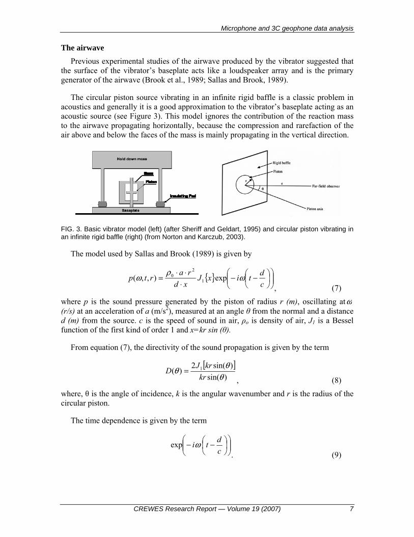
The circular piston source vibrating in an infinite rigid baffle is a classic problem in acoustics and generally it is a good approximation to the vibrator’s baseplate acting as an acoustic source (see Figure 3). This model ignores the contribution of the reaction mass to the airwave propagating horizontally, because the compression and rarefaction of the air above and below the faces of the mass is mainly propagating in the vertical direction.

FIG. 3. Basic vibrator model (left) (after Sheriff and Geldart, 1995) and circular piston vibrating in an infinite rigid baffle (right) (from Norton and Karczub, 2003).

The model used by Sallas and Brook (1989) is given by

{ } ⎟⎟

⎠

⎞⎜⎜⎝

⎛⎟⎠⎞

⎜⎝⎛ −−

⋅⋅⋅

=cdtixJ

xdrartp ωρω exp),,( 1

20

, (7)

where p is the sound pressure generated by the piston of radius r (m), oscillating atω (r/s) at an acceleration of a (m/s2), measured at an angle θ from the normal and a distance d (m) from the source. c is the speed of sound in air, ρo is density of air, J1 is a Bessel function of the first kind of order 1 and x=kr sin (θ).

From equation (7), the directivity of the sound propagation is given by the term

[ ])sin(

)sin(2)( 1

θθθ

krkrJD =

, (8)

where, θ is the angle of incidence, k is the angular wavenumber and r is the radius of the circular piston.

The time dependence is given by the term

⎟⎟⎠

⎞⎜⎜⎝

⎛⎟⎠⎞

⎜⎝⎛ −−

cdtiωexp

. (9)

Alcudia and Stewart


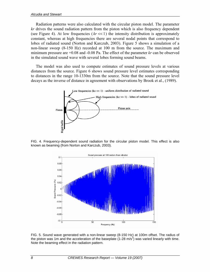
Radiation patterns were also calculated with the circular piston model. The parameter kr drives the sound radiation pattern from the piston which is also frequency dependent (see Figure 4). At low frequencies ( 1<<kr ) the intensity distribution is approximately constant, whereas at high frequencies there are several nodal points that correspond to lobes of radiated sound (Norton and Karczub, 2003). Figure 5 shows a simulation of a non-linear sweep (8-150 Hz) recorded at 100 m from the source. The maximum and minimum pressure are +0.08 and -0.08 Pa. The effect of the parameter kr can be observed in the simulated sound wave with several lobes forming sound beams.

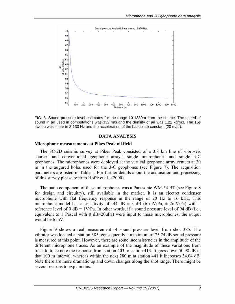
The model was also used to compute estimates of sound pressure levels at various distances from the source. Figure 6 shows sound pressure level estimates corresponding to distances in the range 10-1330m from the source. Note that the sound pressure level decays as the inverse of distance in agreement with observations by Brook et al., (1989).

FIG. 4. Frequency-dependent sound radiation for the circular piston model. This effect is also known as beaming (from Norton and Karczub, 2003).

FIG. 5. Sound wave generated with a non-linear sweep (8-150 Hz) at 100m offset. The radius of the piston was 1m and the acceleration of the baseplate (1-28 m/s2) was varied linearly with time. Note the beaming effect in the radiation pattern.



FIG. 6. Sound pressure level estimates for the range 10-1330m from the source. The speed of sound in air used in computations was 332 m/s and the density of air was 1.22 kg/m3. The 16s sweep was linear in 8-130 Hz and the acceleration of the baseplate constant (20 m/s2).

DATA ANALYSIS

Microphone measurements at Pikes Peak oil field

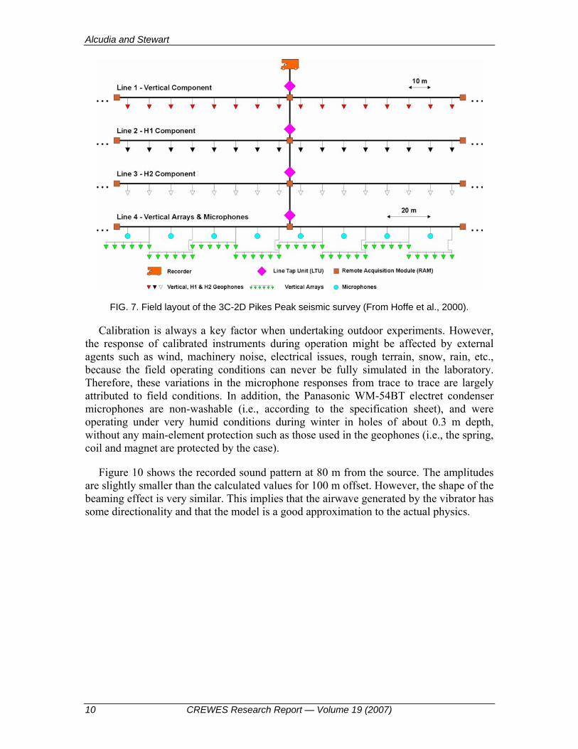
The 3C-2D seismic survey at Pikes Peak consisted of a 3.8 km line of vibroseis sources and conventional geophone arrays, single microphones and single 3-C geophones. The microphones were deployed at the vertical geophone array centers at 20 m in the augured holes used for the 3-C geophones (see Figure 7). The acquisition parameters are listed in Table 1. For further details about the acquisition and processing of this survey please refer to Hoffe et al., (2000).

The main component of these microphones was a Panasonic WM-54 BT (see Figure 8 for design and circuitry), still available in the market. It is an electret condenser microphone with flat frequency response in the range of 20 Hz to 16 kHz. This microphone model has a sensitivity of -44 dB ± 3 dB (6 mV/Pa, ± 2mV/Pa) with a reference level of 0 dB = 1V/Pa. In other words, if a sound pressure level of 94 dB (i.e., equivalent to 1 Pascal with 0 dB=20uPa) were input to these microphones, the output would be 6 mV.

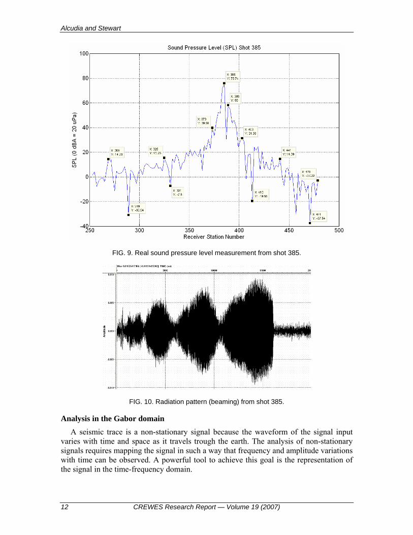
Figure 9 shows a real measurement of sound pressure level from shot 385. The vibrator was located at station 385; consequently a maximum of 75.74 dB sound pressure is measured at this point. However, there are some inconsistencies in the amplitude of the different microphone traces. As an example of the magnitude of these variations from trace to trace note the response from station 403 to station 413. It goes down 50.98 dB in that 100 m interval, whereas within the next 280 m at station 441 it increases 34.04 dB. Note there are more dramatic up and down changes along the shot range. There might be several reasons to explain this.

Alcudia and Stewart


FIG. 7. Field layout of the 3C-2D Pikes Peak seismic survey (From Hoffe et al., 2000).

Calibration is always a key factor when undertaking outdoor experiments. However, the response of calibrated instruments during operation might be affected by external agents such as wind, machinery noise, electrical issues, rough terrain, snow, rain, etc., because the field operating conditions can never be fully simulated in the laboratory. Therefore, these variations in the microphone responses from trace to trace are largely attributed to field conditions. In addition, the Panasonic WM-54BT electret condenser microphones are non-washable (i.e., according to the specification sheet), and were operating under very humid conditions during winter in holes of about 0.3 m depth, without any main-element protection such as those used in the geophones (i.e., the spring, coil and magnet are protected by the case).

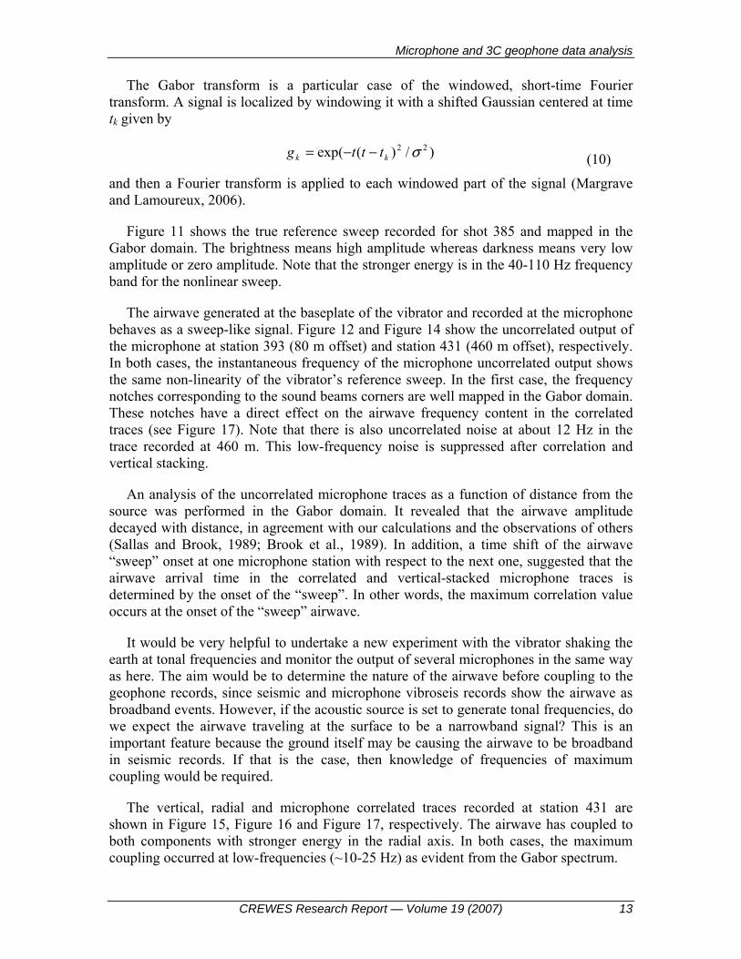
Figure 10 shows the recorded sound pattern at 80 m from the source. The amplitudes are slightly smaller than the calculated values for 100 m offset. However, the shape of the beaming effect is very similar. This implies that the airwave generated by the vibrator has some directionality and that the model is a good approximation to the actual physics.



FIG. 8. The microphones used in this experiment were designed and tested at the University of Calgary. Its power circuit is also shown where two resistors and a condenser are used to regulate the power consumption.

Table 1. Acquisition parameters.

Contractor Veritas DGC Recording system ARAM 24 bits Source 2 HEMI 44 vibrators

25,000 kg each)

Sweeps 4 sweeps, 8-150 Hz, 2 segments, 16 seconds length 1) 0.325 s, 8 - 25 Hz 2) 15.625 s, 25 – 150 Hz

Listening 4 seconds Sampling rate 2 ms Total recording 20 seconds Vibrator spatial area 10 m Source interval 20 m Preamp gain 36 dB Low -cut filter 3 Hz High-cut filter 164 HZ Receiver interval 3C geophones 10 m Receiver interval geophone arrays 20 m Receiver interval microphone 20 m

Alcudia and Stewart


FIG. 9. Real sound pressure level measurement from shot 385.

FIG. 10. Radiation pattern (beaming) from shot 385.

Analysis in the Gabor domain

A seismic trace is a non-stationary signal because the waveform of the signal input varies with time and space as it travels trough the earth. The analysis of non-stationary signals requires mapping the signal in such a way that frequency and amplitude variations with time can be observed. A powerful tool to achieve this goal is the representation of the signal in the time-frequency domain.



The Gabor transform is a particular case of the windowed, short-time Fourier transform. A signal is localized by windowing it with a shifted Gaussian centered at time tk given by

)/)(exp( 22 σkk tttg −−= (10)

and then a Fourier transform is applied to each windowed part of the signal (Margrave and Lamoureux, 2006).

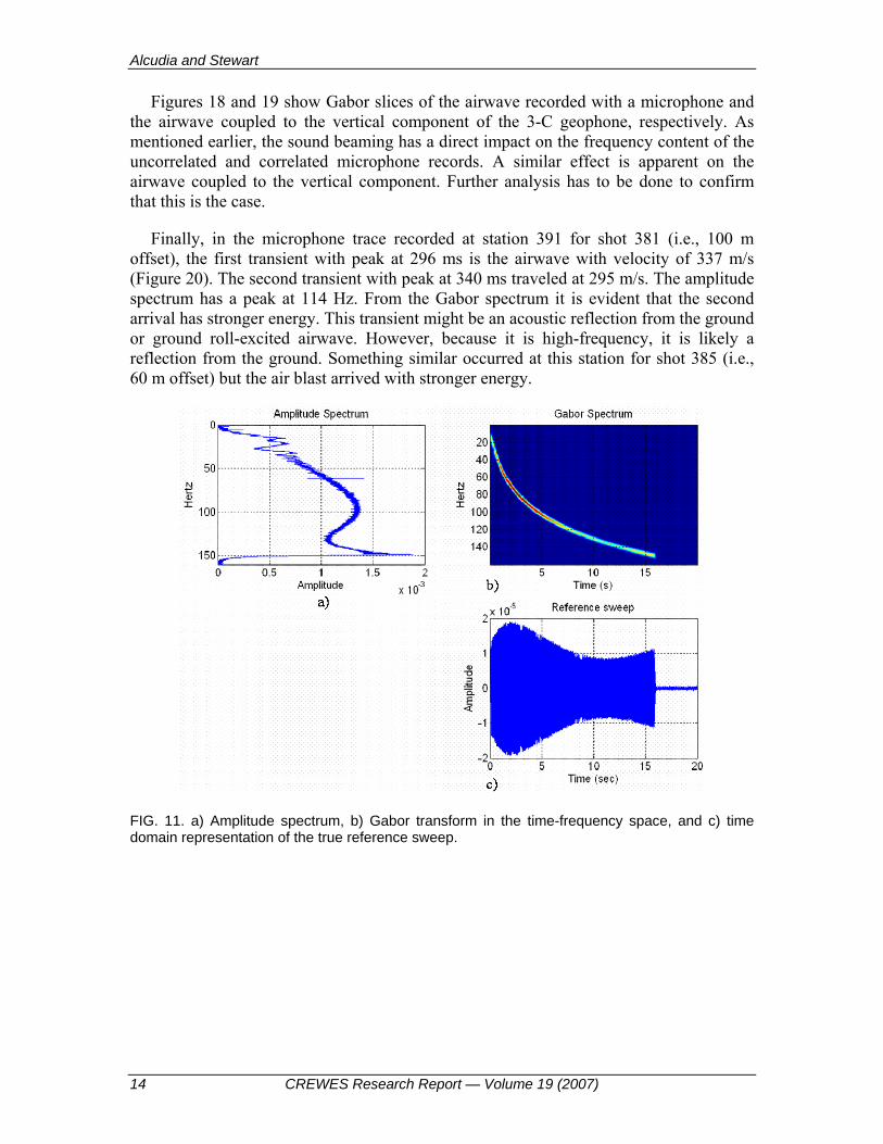
Figure 11 shows the true reference sweep recorded for shot 385 and mapped in the Gabor domain. The brightness means high amplitude whereas darkness means very low amplitude or zero amplitude. Note that the stronger energy is in the 40-110 Hz frequency band for the nonlinear sweep.

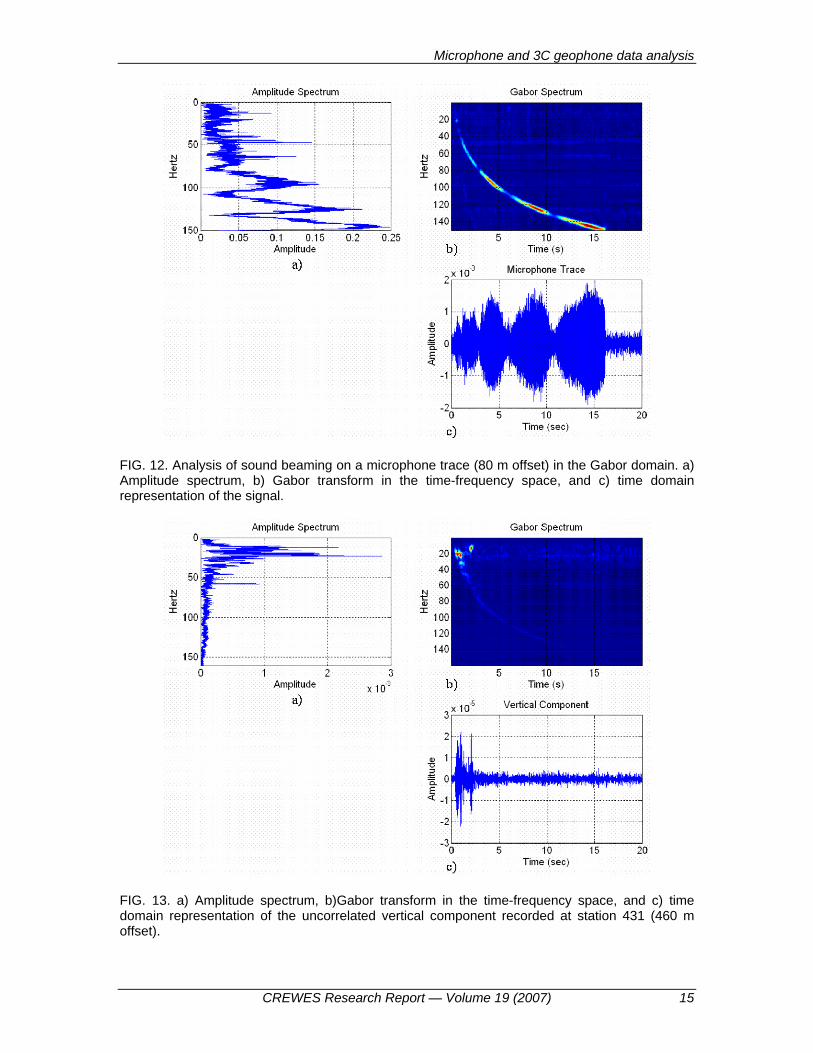
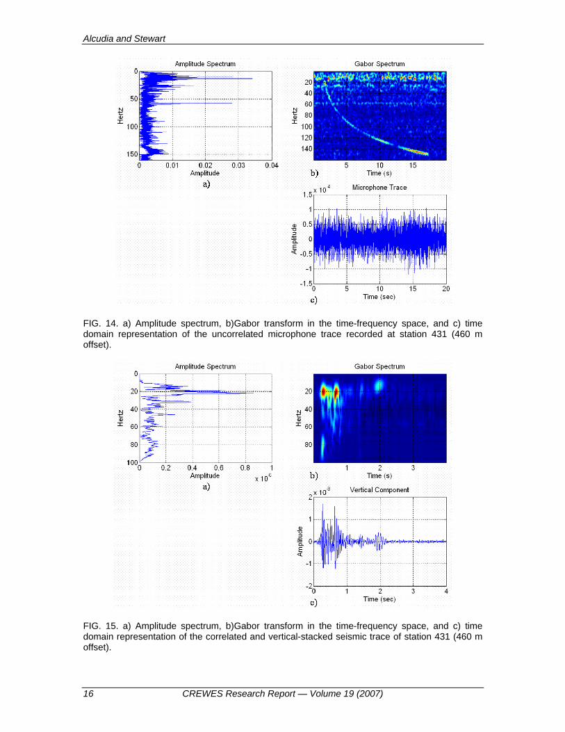
The airwave generated at the baseplate of the vibrator and recorded at the microphone behaves as a sweep-like signal. Figure 12 and Figure 14 show the uncorrelated output of the microphone at station 393 (80 m offset) and station 431 (460 m offset), respectively. In both cases, the instantaneous frequency of the microphone uncorrelated output shows the same non-linearity of the vibrator’s reference sweep. In the first case, the frequency notches corresponding to the sound beams corners are well mapped in the Gabor domain. These notches have a direct effect on the airwave frequency content in the correlated traces (see Figure 17). Note that there is also uncorrelated noise at about 12 Hz in the trace recorded at 460 m. This low-frequency noise is suppressed after correlation and vertical stacking.

An analysis of the uncorrelated microphone traces as a function of distance from the source was performed in the Gabor domain. It revealed that the airwave amplitude decayed with distance, in agreement with our calculations and the observations of others (Sallas and Brook, 1989; Brook et al., 1989). In addition, a time shift of the airwave “sweep” onset at one microphone station with respect to the next one, suggested that the airwave arrival time in the correlated and vertical-stacked microphone traces is determined by the onset of the “sweep”. In other words, the maximum correlation value occurs at the onset of the “sweep” airwave.

It would be very helpful to undertake a new experiment with the vibrator shaking the earth at tonal frequencies and monitor the output of several microphones in the same way as here. The aim would be to determine the nature of the airwave before coupling to the geophone records, since seismic and microphone vibroseis records show the airwave as broadband events. However, if the acoustic source is set to generate tonal frequencies, do we expect the airwave traveling at the surface to be a narrowband signal? This is an important feature because the ground itself may be causing the airwave to be broadband in seismic records. If that is the case, then knowledge of frequencies of maximum coupling would be required.

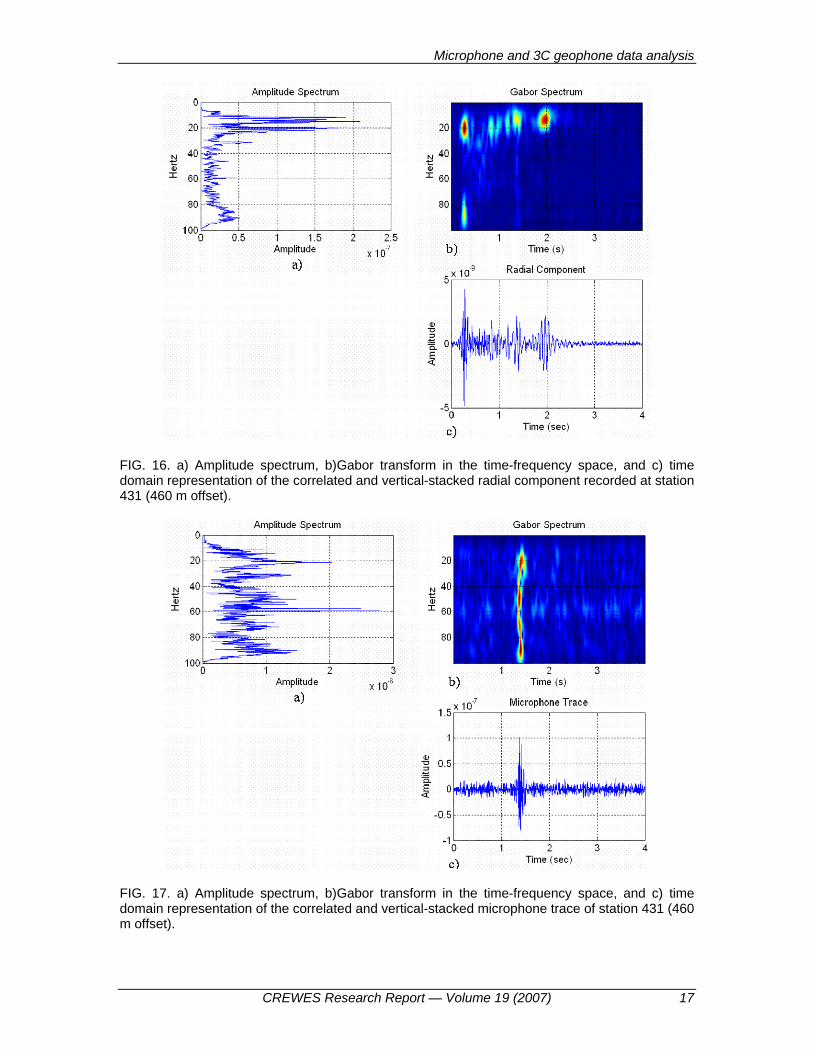
The vertical, radial and microphone correlated traces recorded at station 431 are shown in Figure 15, Figure 16 and Figure 17, respectively. The airwave has coupled to both components with stronger energy in the radial axis. In both cases, the maximum coupling occurred at low-frequencies (~10-25 Hz) as evident from the Gabor spectrum.

Alcudia and Stewart


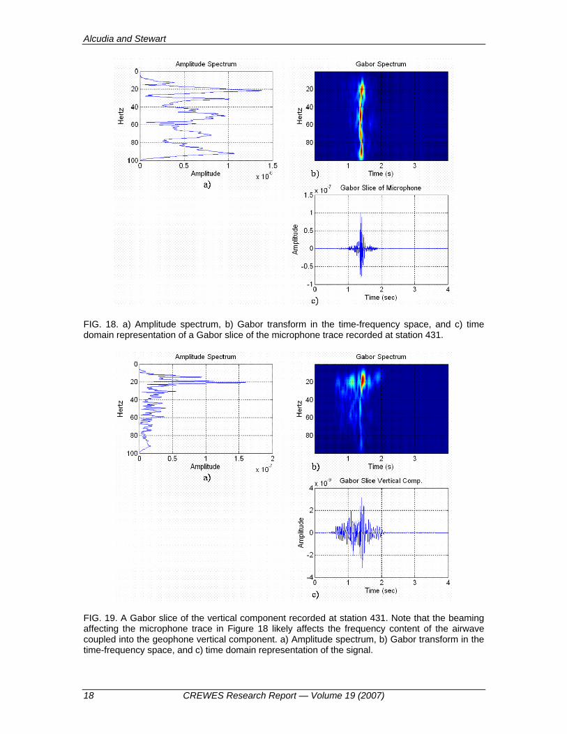
Figures 18 and 19 show Gabor slices of the airwave recorded with a microphone and the airwave coupled to the vertical component of the 3-C geophone, respectively. As mentioned earlier, the sound beaming has a direct impact on the frequency content of the uncorrelated and correlated microphone records. A similar effect is apparent on the airwave coupled to the vertical component. Further analysis has to be done to confirm that this is the case.

Finally, in the microphone trace recorded at station 391 for shot 381 (i.e., 100 m offset), the first transient with peak at 296 ms is the airwave with velocity of 337 m/s (Figure 20). The second transient with peak at 340 ms traveled at 295 m/s. The amplitude spectrum has a peak at 114 Hz. From the Gabor spectrum it is evident that the second arrival has stronger energy. This transient might be an acoustic reflection from the ground or ground roll-excited airwave. However, because it is high-frequency, it is likely a reflection from the ground. Something similar occurred at this station for shot 385 (i.e., 60 m offset) but the air blast arrived with stronger energy.

FIG. 11. a) Amplitude spectrum, b) Gabor transform in the time-frequency space, and c) time domain representation of the true reference sweep.



FIG. 12. Analysis of sound beaming on a microphone trace (80 m offset) in the Gabor domain. a) Amplitude spectrum, b) Gabor transform in the time-frequency space, and c) time domain representation of the signal.

FIG. 13. a) Amplitude spectrum, b)Gabor transform in the time-frequency space, and c) time domain representation of the uncorrelated vertical component recorded at station 431 (460 m offset).

Alcudia and Stewart


FIG. 14. a) Amplitude spectrum, b)Gabor transform in the time-frequency space, and c) time domain representation of the uncorrelated microphone trace recorded at station 431 (460 m offset).

FIG. 15. a) Amplitude spectrum, b)Gabor transform in the time-frequency space, and c) time domain representation of the correlated and vertical-stacked seismic trace of station 431 (460 m offset).



FIG. 16. a) Amplitude spectrum, b)Gabor transform in the time-frequency space, and c) time domain representation of the correlated and vertical-stacked radial component recorded at station 431 (460 m offset).

FIG. 17. a) Amplitude spectrum, b)Gabor transform in the time-frequency space, and c) time domain representation of the correlated and vertical-stacked microphone trace of station 431 (460 m offset).

Alcudia and Stewart


FIG. 18. a) Amplitude spectrum, b) Gabor transform in the time-frequency space, and c) time domain representation of a Gabor slice of the microphone trace recorded at station 431.

FIG. 19. A Gabor slice of the vertical component recorded at station 431. Note that the beaming affecting the microphone trace in Figure 18 likely affects the frequency content of the airwave coupled into the geophone vertical component. a) Amplitude spectrum, b) Gabor transform in the time-frequency space, and c) time domain representation of the signal.



FIG. 20. Microphone trace at 100 m offset with two strong arrivals corresponding to the airwave and likely a reflection from the ground. a) Amplitude spectrum, b)Gabor transform in the time-frequency space, and c) time domain representation of the signal.

CONCLUSIONS

Coupling phenomena associated to energy conversion at the air-ground interface could be better understood if pressure levels and particle velocity, displacement or acceleration amplitudes are recorded at the field. For instance, the frequency content of the sound wavefield emanating from the vibrator’s baseplate is affected by its radiation pattern. This effect was successfully recorded by the microphones at the near-field (at offsets <200m). Preliminary analysis of the geophone components in the Gabor domain suggested that sound beaming might also impact the frequency content of the coupled airwave.

FUTURE WORK There is plenty of room for research on co-located pressure and ground motion sensors

and their potential applications. Future research at the CREWES project will use this dual-sensor approach to characterize the ground response to seismic sources. Seismic operations would benefit from a priori knowledge of the ground response close to sensitive or restricted areas.

Another research direction consists of using polarization analysis along with microphone and 3-C seismic data to characterize the ground roll and its interaction with traveling acoustic waves at the surface. Hodograms provide a visual analysis of the particle motion along a trajectory. To measure the angle of direction and linearity, other methods of polarization analysis have to be included such as histograms and covariance matrix. A feasible study about ground roll characterization would require the three

Alcudia and Stewart


methods. A more complex modeling of these phenomena is mandatory. Therefore, finite-difference modeling of acoustic and elastic waves interacting at the air-ground interface will be considered.

ACKNOWLEDGEMENTS

We would like to thank the Alberta Oil Sands Technology and Research Authority (AOSTRA) and Husky Energy Inc. for their financial support of this project. We also thank CREWES sponsors and staff for their continuing support.

REFERENCES Brook, R.A., Crews, G.A. and Sallas, J.J., 1989, Experimental analysis of the vibrator air wave: 59th Ann.

Internat. Mtg., Soc. Expl. Geophys., Expanded Abstracts, 683-685. Dey, A.K., Stewart, R.R., Lines, L.R. and Bland, H.C., 2000, Noise suppression on geophone data using

microphone measurements: CREWES Research Report, 12. Haskell, N.A., 1951, A note on air-coupled surface waves: Bulletin of the Seismological Society of

America, 41, 295-300. Hill, D.P., Fischer, F.G., Lahr, K.M., and Coakley, J.M., 1976, Earthquake sounds generated by body-wave

ground motion: Bulletin of the Seismological Society of America, 66, 4, 1159-1172. Hoffe. B.H., Bertram, M.B., Bland, H.C., Gallant, E.V., Lines, L.R., and Mewhort, L.E., 2000, Acquisition

and processing of the Pikes Peak 3C-2D seismic survey: CREWES Research Report 12. Jardetzky, W.S. and Press, F., 1952, Rayleigh-wave coupling to atmospheric compression waves: Bulletin

of the Seismological Society of America, 42, 135-144. Le Pichon, A., Guilbert, J., Vega, A., Garcés, M., and Brachet, N., 2001, Ground-coupled airwaves and

diffracted infrasound from the Arequipa earthquake of June 23, 2001: Geophysical Research Letters, 29, 18, 33-1 – 33-4.

Margrave, G.F. and Lamoureux, M.P., 2006, Gabor Deconvolution: CSEG Recorder, 2006 Special Edition, 30-36.

Mooney, H.M. and Kaasa, R.A., 1962, Air waves in engineering seismology: Geophysical Prospecting, 10, 84-9.

Norton, M. and Karczub, 2003, Fundamentals of noise and vibration analysis for engineers: Cambridge University Press.

Press, F. and Ewing, M., 1951, Ground roll coupling to atmospheric compressional waves: Geophysics, 16, 416-430.

Press, F. and Oliver, J., 1955, Model study of air-coupled surface waves: Journal of the Acoustical Society of America, 27, 43-46.

Sallas, J.J. and Brook, R.A., 1989, Air-coupled noise produced by a seismic P-wave vibrator: 59th Ann. Internat. Mtg., Soc. Expl. Geophys., Expanded Abstracts, 686-689.

Sheriff, R.E. and Geldart, L.P., 1995, Exploration Seismology: Cambridge University Press.

analysis of microphone and 3c geophone measurements from a ... · microphone and 3c geophone data...

Documents