analysis of large data sets: bayesian methods and
TRANSCRIPT

Analysis of large data sets:Bayesian methods and applicationsin energy and health economics
Dissertation
zur
Erlangung des Doktorgrades
Dr. rer. pol.
der Fakultat fur Wirtschaftswissenschaftender Universitat Duisburg-Essen
vorgelegt von
Matthias Kaeding
aus Gottingen
Betreuer:Prof. Dr. Christoph HanckLehrstuhl fur Okonometrie
Essen, Juli 2020

Gutachter:Prof. Dr. Christoph HanckProf. Dr. Dr. h. c. Christoph M. Schmidt
Tag der mundlichen Prufung: 01.02.2021
Diese Dissertation wird via DuEPublico, dem Dokumenten- und Publikationsserver derUniversität Duisburg-Essen, zur Verfügung gestellt und liegt auch als Print-Version vor.
DOI:URN:
10.17185/duepublico/74250urn:nbn:de:hbz:464-20210615-105920-4
Dieses Werk kann unter einer Creative Commons Namensnennung -Nicht kommerziell - Keine Bearbeitungen 4.0 Lizenz (CC BY-NC-ND 4.0) genutzt werden.

If if if... doesn‘t exist.RAFAEL NADAL

4

Preface
I wrote this thesis while working at the Research Data Center at the RWI – LeibnizInstitute for Economic Research, half of the essays are written in conjunctionwith colleagues from the RWI. I want to thank several people essential in writingof this thesis:
• I owe my deepest gratitude to my Ph.D. advisor Christoph Hanck for hisexcellent supervision, his very helpful, thorough and fast feedback and thefreedom in choosing my research topics.
• I am very grateful to Christoph M. Schmidt for being my second supervisorand for creating a stimulating and open research environment at the RWI,from which I benefited extensively.
• I would like to thank everyone at the Research Data Center for helpfuldiscussions, in particular Philipp Breidenbach and Sandra Schaffner.
• Furthermore, I would like to thank my office mates Fabian Dehos and LeaEilers for helpful comments and lots of great talks.
• Thank you to all my coauthors: Manuel Frondel, Alexander Haering,Stephan Sommer and Anna Werbeck, who taught me a lot about theirrespective fields and who allowed me to benefit from their expertise andideas.
• Special thanks to my parents Ingeburg and Jurgen, and to my sister Laura.
• Most importantly, I thank Rilana. For everything.
5

6

Contents
1 Introduction 9
2 Technical preliminaries 132.1 Bayesian inference . . . . . . . . . . . . . . . . . . . . . . . . . . 13
2.1.1 Metropolis-Hastings algorithm . . . . . . . . . . . . . . . 132.1.2 Point and interval estimation . . . . . . . . . . . . . . . . 15
2.2 Set cover problem . . . . . . . . . . . . . . . . . . . . . . . . . . 15
I Bayesian methods 17
3 Efficient Bayesian nonparametric hazard regression 193.1 Introduction . . . . . . . . . . . . . . . . . . . . . . . . . . . . . . 203.2 Hazard regression model . . . . . . . . . . . . . . . . . . . . . . . 20
3.2.1 Priors . . . . . . . . . . . . . . . . . . . . . . . . . . . . . 223.2.2 Likelihood construction . . . . . . . . . . . . . . . . . . . 25
3.3 Inference . . . . . . . . . . . . . . . . . . . . . . . . . . . . . . . . 263.3.1 Model choice . . . . . . . . . . . . . . . . . . . . . . . . . 273.3.2 Covariate effects . . . . . . . . . . . . . . . . . . . . . . . 27
3.4 Simulation study . . . . . . . . . . . . . . . . . . . . . . . . . . . 293.5 Application: Real estate data . . . . . . . . . . . . . . . . . . . . 313.6 Conclusion . . . . . . . . . . . . . . . . . . . . . . . . . . . . . . 33
4 Fast, approximate MCMC for Bayesian analysis of large datasets: A design based approach 354.1 Introduction . . . . . . . . . . . . . . . . . . . . . . . . . . . . . . 364.2 Noisy Metropolis-Hastings . . . . . . . . . . . . . . . . . . . . . . 364.3 Some sampling theory . . . . . . . . . . . . . . . . . . . . . . . . 38
4.3.1 Sampling design: Cube sampling . . . . . . . . . . . . . . 384.3.2 Regression estimator . . . . . . . . . . . . . . . . . . . . . 40
4.4 Description of algorithm . . . . . . . . . . . . . . . . . . . . . . . 414.4.1 Ridge variant . . . . . . . . . . . . . . . . . . . . . . . . . 43
4.5 Simulation study . . . . . . . . . . . . . . . . . . . . . . . . . . . 434.5.1 Setup . . . . . . . . . . . . . . . . . . . . . . . . . . . . . 434.5.2 Results . . . . . . . . . . . . . . . . . . . . . . . . . . . . 44
4.6 Application . . . . . . . . . . . . . . . . . . . . . . . . . . . . . . 474.7 Discussion . . . . . . . . . . . . . . . . . . . . . . . . . . . . . . . 484.A Appendix . . . . . . . . . . . . . . . . . . . . . . . . . . . . . . . 50
7

CONTENTS
II Applications in energy and health economics 51
5 Market premia for renewables in Germany: The effect on elec-tricity prices 535.1 Introduction . . . . . . . . . . . . . . . . . . . . . . . . . . . . . . 545.2 Germany’s Market Premium for RES . . . . . . . . . . . . . . . . 555.3 Data . . . . . . . . . . . . . . . . . . . . . . . . . . . . . . . . . . 595.4 Method . . . . . . . . . . . . . . . . . . . . . . . . . . . . . . . . 605.5 Results . . . . . . . . . . . . . . . . . . . . . . . . . . . . . . . . . 645.6 Conclusion . . . . . . . . . . . . . . . . . . . . . . . . . . . . . . 675.A Appendix . . . . . . . . . . . . . . . . . . . . . . . . . . . . . . . 69
6 Equal access to primary care: A benchmark for spatial allocation 736.1 Introduction . . . . . . . . . . . . . . . . . . . . . . . . . . . . . . 746.2 Data . . . . . . . . . . . . . . . . . . . . . . . . . . . . . . . . . . 756.3 Methodology . . . . . . . . . . . . . . . . . . . . . . . . . . . . . 786.4 Results . . . . . . . . . . . . . . . . . . . . . . . . . . . . . . . . . 846.5 Sensitivity analysis . . . . . . . . . . . . . . . . . . . . . . . . . . 886.6 Conclusion . . . . . . . . . . . . . . . . . . . . . . . . . . . . . . 896.A Appendix . . . . . . . . . . . . . . . . . . . . . . . . . . . . . . . 91
7 Conclusion 93
8

Chapter 1
Introduction
The availability of large data sets is increasing dramatically, reshaping decision-making in many domains, such as energy, education and health. Data sets maybe large in two dimensions: in the number of observations and in the numberof variables. This thesis mainly deals with the first case. For the purpose ofthis dissertation a data set is large when its size causes problems for statisticalinference. Such data sets may consist of structured data, where the distinctionbetween observation and variable is clear, such as insurance data or high resolutionpopulation data. Large data sets may also consist of unstructured data, such asdata from social networks sites or news articles.
Often, large data sets arise as a byproduct of emerging technologies, possiblyallowing very detailed measurements in space or time. For instance, currentcontinuous glucose monitoring systems measure blood sugar levels every fiveminutes, while smartphone data may provide precise information on the locationof persons. It is common that large data sets provide information on everyelement of interest, instead of a subsample of elements. For instance, Germangas stations are required by law to report gas prices immediately, resultant in adata set giving nearly complete price information.
While existing statistical methods were not developed for small data setsper se, their direct application to large data sets is often problematic, eventhough many methods are justified by large sample asymptotics. These problemsmay be inferential, for instance common testing procedures may break downin practice. This thesis is mainly concerned with computational problems, ascommon estimation algorithms are often too time or memory consuming to usewith large data sets.
The analysis of large data sets using the appropriate methodology allowsresearchers to ask new kinds of research questions or to recast old ones, benefitingfrom the resultant statistical precision. Furthermore, large data methods offeruseful tools to solve applied problems.
This thesis aims to contribute to the statistical analysis of large data sets.These contributions are twofold: First, this thesis lightens the computationaldemands of existing methods, improving applicability to large-scale problems.Second, this thesis uses large data methods to solve problems with importantpolicy implications in energy and health economics. Consequently, this thesis isdivided into a methodological and an econometric part, where each part consistsof two essays.
The first part consists of two single-authored essays developing statisticalmethods for Bayesian analysis of large data sets: Somewhat paradoxically, large-scale inference often involves including additional information to obtain useful
9
estimates. Consider the estimation of a flexible regression model with nonlinearor spatial components. Such a model may involve a high dimensional parametervector and may require a large data set. Here, imposing some structure on theestimates via regularization improves or enables inference. For instance, shrinkingregression coefficients towards zero, or setting some exactly to zero, allows estima-tion of regression coefficients when the number of covariates exceeds the numberof observations. In this case, an unadjusted least squares estimator is unusable.Another important example is function estimation via splines, where reducingdeviations of neighboring spline coefficients leads to more realistic function esti-mates. Bayesian inference offers a natural way to incorporate regularization viathe prior distribution, representing prior knowledge. As such, Bayesian inferenceis well-equipped to handle large-scale problems in theory. However, existingBayesian methods are often computationally too demanding for such problems.The essays in the first part of this thesis aim to decrease computational demandsof Bayesian methods: Chapter 3 streamlines Bayesian hazard regression, Chapter4 accelerates a simulation algorithm of central importance for Bayesian inference.
The second part of this thesis consists of two co-authored essays in healthand energy economics. The studies apply large data methods to research ques-tions with important policy implications and thus demonstrate the potentialof applying these new developments to economic policy debates. In particular,the second part answers questions that could not be answered without access tonew data and methods developed for large data sets: Chapter 5 requires preciseprediction of negative electricity prices, which occur very rarely. To achievethis, the chapter uses a machine learning model. Chapter 6 involves the use ofa fast approximation algorithm to determine an optimal allocation of generalpractitioners on a small scale in Germany. The remainder of this introductionsummarizes each essay, Chapter 2 gives technical preliminaries necessary for theessays.
Chapter 3 accelerates and simplifies inference for Bayesian hazard regression. Thehazard rate gives the instantaneous rate of failure at t, conditional on survivaluntil t and covariate values of zero. Important applications of hazard regressionare the analysis of unemployment durations or the modeling of time until death.Covariate effects for hazard regression are hard to interpret, Bayesian approachesare computationally expensive. Usually no closed form expression for the hazardregression likelihood is available, requiring an approximation which may be ex-pensive to compute. This chapter aims to alleviate these problems by modelingthe integrated baseline hazard via monotonic penalized B-splines (P-splines).B-splines are functions, formed from connected local polynomials. The basic ideaof Bayesian P-splines is to model an unknown function via a weighted sum ofB-splines, controlling smoothness via an estimated penalty parameter.
The presented modeling strategy gives a closed form expression for thelikelihood, allows accounting for arbitrary censorship and the inclusion of furthernonparametric components modeled by P-splines. Because of the good numericalproperties of B-splines, involved computations are fast and stable. Furthermore,the computational advantages allow easy effect interpretation by combination oftwo concepts: Partial dependence plots show the relationship between a covariateand an estimand, marginalizing over all covariates except the one of interest.Here, the estimand is the restricted mean survival time, easy to compute in thepresented framework. This allows effect interpretation in terms of survival timesinstead of the hazard rate.
10

1 Introduction
Monte Carlo simulations show that the modeling strategy works well, if thesample size is large enough. An application using a large real estate data setshows that the presented methods give useful results in practice.
Chapter 4 develops a fast, approximate Metropolis-Hastings algorithm for Bayesiananalysis of large data sets. Because the Metropolis-Hastings algorithm allowssampling from the posterior distribution if no complete analytic expression isavailable, the algorithm is of central importance in Bayesian statistics. Runningthe algorithm involves computation of loglikelihood-ratio sums, so that the runtime of the algorithm is usually linear in the sample size. This makes inferencewith large data sets impractical. The chapter proposes a fast approximationembedded in a sampling design framework, which is concerned with the esti-mation of finite population sums. Here, the outcome of interest is the sum ofloglikelihood-ratio differences.
The presented algorithm is based on a single subsample, bypassing the needto store the complete data set. The subsample is taken via the cube method, abalanced sampling method where a random sample is drawn so that the meanof a set of auxiliary variables is close to the population mean. This reduces thevariance of the sample mean, if the auxiliary variables are correlated with theoutcome variable. Here, the auxiliary variables satisfy this condition by design.Furthermore, presence of the auxiliary variables allows using variants of theregression estimator: This estimator uses the auxiliary information to predictthe estimation error, which is subtracted from the estimate.
An application using a data set consisting of 31 million rows and simulationstudies show that the presented approach can lead to a strong reduction incomputation time. Results are very close to those obtained using the completedata set.
Chapter 5, co-authored by Manuel Frondel and Stephan Sommer, models theeffect of the introduction and amendment of a market premia scheme on theoccurrence of negative electricity prices. In Germany, plant operators usingrenewable technologies could obtain guaranteed fixed payments. As this so-calledfeed-in-tariff is paid independent of the market price of electricity, it may resultin negative prices when high electricity supply coincides with low demand, forinstance in the morning hours or during national holidays.
Energy oversupply causes negative electricity prices, in turn causing instabilityof the electricity grid, increasing grid maintenance cost. Furthermore, negativeelectricity prices induce welfare losses: Because of substantial ramp-up costs,providers of conventional plants usually do not halt production when revenuesare negative. The increasing share of electricity from renewable energy sourcesmagnifies these problems. To counteract, a market premia scheme was introduced,aiming to align electricity production with demand. The market premia schemecreates incentives for plant operators to sell electricity directly to customers atvariable wholesale prices, instead of a fixed price.
Because of the small share of negative prices overall (less than one percent),and due to the presence of nonlinear interactions, common statistical methodsmay fail in predicting negative prices. Consequently, our modeling strategyis based on Bayesian Additive Regression Trees (BART), a machine learningtechnique known to perform well in such settings. We find that BART preciselyidentifies potential negative price spikes, unlike common methods such as linearregression. We use the BART model to simulate electricity prices under coun-
11

terfactual settings, finding that the introduction of a market premia scheme isassociated with a reduction of negative electricity prices by some 70%.
Chapter 6, co-authored by Alexander Haering and Anna Werbeck, creates abenchmark for the spatial allocation of general practitioners (GPs) in Germany.Unlike existing approaches, we use a large data set with detailed populationinformation for 1km2 grids with information on the current allocation of GPs.Furthermore, we use realistic estimates of driving times, incorporating detailedroad information. Based on German regulation, an optimal allocation minimizesthe number of GPs under two constraints: Every person reaches at least one GPby car in less than 15 minutes, and no GP services more than 13,000 patient visitsper year. Because of the high dimensionality of the solution set, determinationof the optimal allocation is not feasible. Instead, we use a fast approximationalgorithm.
For all Germany, we find a deficit in GPs of some 6%. Using a spatial linear re-gression model, we analyze regional patterns by comparing the optimal allocationwith the status quo. We use two indices defined on a municipality level: numberof excess GPs (supply side) and percentage of uncovered cases (demand side). Wefind a surplus of GPs in cities, compared to rural and suburban municipalities.However, this does not translate to the demand side, where we do not find anassociation of healthcare demand with density.
The remainder of this thesis is structured as follows: Chapter 2 gives technicalpreliminaries, Chapters 3 to 6 give the main results. Chapter 7 concludes.
12

Chapter 2
Technical preliminaries
2.1 Bayesian inference
Let θ ∈ Θ denote the parameter vector of interest and D denote the data.The probability density function of θ, conditional on D, the so-called posteriordistribution, is the basis for Bayesian inference. The posterior distribution p(θ|D)arises by combining the prior distribution p(θ), representing available informationabout θ before seeing the data, with the likelihood L(θ|D). This gives
p(θ|D) = kL(θ|D)p(θ),
with normalizing constant
k :=(∫
L(θ|D)p(θ) dθ)−1
.
The crucial steps for Bayesian inference are the choice of prior and likelihood,and the summary of the resultant posterior distribution. For a comprehensiveoverview of Bayesian inference see Gelman, Carlin, Stern, Dunson, Vehtari, andRubin (2013) or Robert (2001).
2.1.1 Metropolis-Hastings algorithm
In practice, the proportionality constant k is usually unknown except for verysimple models, so that the posterior distribution is not fully available. As analternative, Markov chain Monte Carlo (MCMC) methods create a sequence ofparameter draws θ(1), . . . ,θ(T ), which mimic samples drawn from the posteriordistribution. Inference is then based on those parameter draws, which forma Markov chain: the distribution of θ(t) given θ(t−1), . . . ,θ(1) depends only onθ(t−1). It holds that
P (θ(t) ∈ A|θ(t−1), . . . ,θ(1)) = P (θ(t) ∈ A|θ(t−1)) =∫AK(θ(t)|θ(t−1))dθ(t),
where the transition kernel K(θ(t)|θ(t−1)) denotes the conditional density of θ(t),given θ(t−1). The transition kernel is a representation of a Markov chain, it ischosen so that output of the chain mimics output from the posterior distribution.To achieve this, the invariant distribution of the Markov chain must be theposterior distribution p(θ|D), then
p(θ(t)|D) =∫K(θ(t)|θ(t−1))p(θ(t−1)|D)dθ(t−1) (2.1)
13

2.1 Bayesian inference
holds. It follows from equation (2.1) that, if θ(t) is sampled from the posteriordistribution, all subsequent samples are as well. Detailed balance
p(θ(t)|D)K(θ(t−1)|θ(t)) = p(θ(t−1)|D)K(θ(t)|θ(t−1)) (2.2)
is a sufficient, but not necessary condition to ensure the posterior distribution asinvariant distribution of a Markov chain. This follows by integrating equation(2.2) over θ(t−1). Then, the left hand side becomes∫p(θ(t)|D)K(θ(t−1)|θ(t))dθ(t−1) = p(θ(t)|D)
∫K(θ(t−1)|θ(t))dθ(t−1) = p(θ(t)|D),
(2.3)
since K is a density, so that the condition in (2.1) is satisfied. See Andrieu,De Freitas, Doucet, and Jordan (2003) or Robert and Casella (2004) for anintroduction to Markov chain Monte Carlo methods.
This thesis uses as main MCMC method the Metropolis-Hastings algorithm,or variants thereof. The algorithm allows obtaining draws from a density onlyknown up to a proportionality, such as the posterior distribution. The mainingredient is the proposal distribution g, from which one can sample. Whenused for the simulation of the posterior distribution, the Metropolis-Hastingsalgorithm consists of the following steps:
1. Choose start values θ(0) and proposal distribution g
2. For t = 1, . . . , T :
• Draw a proposal θ? from g(θ?|θ(t−1))• Compute
α(θ(t−1),θ?) = min(
1, p(θ?|D)g(θ(t−1)|θ?)p(θ(t−1)|D)g(θ?|θ(t−1))
),
Accept the proposal with probability α(θ(t−1),θ?); set θ(t) = θ?.Otherwise, reject the proposal; set θ(t) = θ(t−1).
3. Return θ(1), . . . ,θ(T )
The normalizing constant k, cancels out in the acceptance ratio α(·, ·), so that kmay be unknown, for instance k = (2
√π)−1 for a standard normal distribution.
The transition kernel of the Metropolis-Hastings algorithm is
KMH(θ(t)|θ(t−1)) =g(θ(t)|θ(t−1))α(θ(t−1),θ(t))+ (2.4)
I[θ(t) = θ(t−1)]∫g(θ?|θ(t−1))
(1− α(θ(t−1),θ?)
)dθ?, (2.5)
where the right hand side of equation (2.4) corresponds to acceptance, andequation (2.5) corresponds to rejection of a proposal. The kernel satisfies thedetailed balance condition, so that the posterior distribution is the invariantdistribution of the chain.
Chapter 5 uses the popular Gibbs sampler to draw from the posterior distri-bution. Let
θ(t)−i := (θ(t)
1 , θ(t)2 , . . . , θ
(t)i−1, θ
(t−1)i+1 , . . . , θ
(t−1)I )>
denote the parameter vector, without the subvector i, at iteration t while runninga Gibbs-sampler. The main requirement for use of the Gibbs sampler is the
14

2 Technical preliminaries
ability to draw from the conditional density p(θ(t)i |θ
(t)−i ,D) for i = 1, . . . , I, i.e., the
posterior distribution of the subvector θ(t)i , conditional on all other parameters.
The sampler iterates the following steps:
1. Choose start values θ(0)
2. For t = 1, . . . , T :
• For i = 1, . . . , I:– Draw θ
(t)i from p(θ(t)
i |θ(t)−i ,D)
3. Return θ(1), . . . ,θ(T )
The Gibbs sampler is a special case of the Metropolis-Hastings algorithm withproposal distribution p(θ(t)
i |θ(t)−i ,D).
2.1.2 Point and interval estimation
Under the Bayesian decision theoretical approach, point estimators arise bydefining a loss function l(γ,θ), and minimizing the posterior expected loss∫
Θl(γ,θ)p(θ|D) dθ, (2.6)
where γ is the true parameter vector. Because γ is unknown, the Bayesianapproach integrates over the parameter space Θ, weighting the loss l(γ,θ) viathe posterior distribution of the unknown parameters, conditional on the knowndata. See Robert (2001) or Lehmann and Casella (1998) for decision-theoreticbackground of Bayesian statistics. The choice of loss function determines theestimator as minimizer of (2.6). This thesis uses mainly the posterior meanas point estimate, corresponding to quadratic loss l(γ,θ) = (θ − γ)2. Anotherpopular choice is the posterior median, corresponding to absolute loss.
Using MCMC output, an estimator is computed from its empirical equivalent,e.g. the average
T−1T∑t=1
h(θ(t)) (2.7)
is used to estimate the posterior mean of some function h(θ). The most commoncase is h(θ) = θ, but sometimes h is more complex: in Chapter 3, one quantityof interest is h(θ) = exp(− exp(b>θ)). If some regulatory conditions are satisfied,averages such as (2.7) converge to the expectation Ep(θ|D)[h(θ)].
Posterior intervals are used to communicate uncertainty. Interval estimates arederived in analogy to point estimators from simulation output: We can estimatethe interval [L,U ], so that P (h(θ) > L) = P (h(θ) < U) = α, via the intervalformed by the α and 1−α quantile from the simulated values h(θ(1)), . . . , h(θ(T )).
2.2 Set cover problem
The set cover problem is a problem from combinatorics with wide rangingapplications such as personnel shift planning, virus detection or location planning.It is of central importance in the field of approximation algorithms, becausemany problems can be cast as set cover problem instance or relate directly tothe problem. This is the case for Chapter 6, where a variant of the set coverproblem is applied to finding an allocation of general practitioners in Germany.
15

2.2 Set cover problem
The set cover problem presents as follows: The input is a collection of setsS = {S1, . . . , Sn} with cost (or weight) function c : S → R≥0. The collection Scovers a universe U , i.e.,
S1 ∪ S2 ∪ · · · ∪ Sn = U .
The aim is to find the minimal cost subcollection X ⊆ S, so that X covers U .For the unweighted set cover problem, it holds that
c(S1) = c(S2) = · · · = c(Sn),
so X is the subcollection with the smallest number of sets, covering U . Foran overview of the problem see Korte and Vygen (2018) or Vazirani (2001).Because the solution set is finite, one can always find the optimal solution to theproblem in theory, for instance by brute force or linear programming. However,in practice the size of the solution often makes this infeasible due to the resultantcomputational demands. It turns out that a greedy approximation algorithmgives a solution, which is hard to improve. The basic idea of the approximationis to find the set with highest cost-effectiveness in each iteration. The algorithmconsists of the following steps:
1. Set C = {} and X = {}
2. While X does not cover U :
• Find the set R with the least cost per uncovered element, i.e. the setwith smallest value of
c(R)|R− C|
, given that |R− C| > 0,
where |R− C| denotes the cardinality of the set R− C.• Set C = C ∪R and X = X ∪ {R}
3. Return X
For the unweighted case, the set with the highest cost-effectiveness is alwaysthe set with the largest number of uncovered elements. Let OPT(U ,S, c) be thecost of the optimal solution for a problem instance with universe U , collection Sand cost function c. Chvatal (1979) shows that the cost of the solution from thegreedy approximation is bounded from above by the factor
OPT(U ,S, c)[1 + 1
2 + . . .1R
]where R := max(|S1|, |S2|, . . . , |Sn|) and |Si| denotes the cardinality of Si. Vazi-rani (2001, chap. 29) shows rigorously why it is very hard to improve upon thesomewhat obvious greedy approximation algorithm.
16

Part I
Bayesian methods
17


Chapter 3
Efficient Bayesiannonparametric hazardregression1
Abstract
We model the log-cumulative baseline hazard for the Cox model via Bayesian,monotonic P-splines. This approach permits fast computation, accounting forarbitrary censorship and the inclusion of nonparametric effects. We leverage thecomputational efficiency to simplify effect interpretation for metric and non-metricvariables by combining the restricted mean survival time approach with partialdependence plots. This allows effect interpretation in terms of survival times.Monte Carlo simulations indicate that the proposed methods work well. Weillustrate our approach using a large data set of real estate data advertisements.
Keywords: Bayesian survival analysis; Nonparametric modeling; Penalizedspline; Restricted mean survival time
1This chapter has been published as: Kaeding, M. (2020). Efficient Bayesian nonparametrichazard regression. Ruhr Economic Papers, 850, 1–21. doi:10.4419/86788985
19

3.1 Introduction
3.1 Introduction
In economic, epidemiological and engineering applications, the Cox proportionalhazards model is the benchmark for survival analysis. However, nonparametricmodeling strategies for the Cox model do not scale up to large data sets. Thispaper aims to alleviate this problem by speeding up computation. The baselinehazard h0(t) is the key concept for the Cox model. It gives the instantaneousrate of failure at t, conditional on survival until t and covariate values of zero.We propose to model the log-integrated baseline hazard via Bayesian, monotonicpenalized B-splines. As we can evaluate the likelihood analytically, and due tothe benefits of Bayesian P-splines, our approach holds five key advantages: (1)Fast, automatic computation. (2) Exact likelihood calculation. (3) Accountingfor arbitrary censoring. (4) Inclusion of nonparametric components. (5) Easiereffect interpretation in regards to survival times, not hazard rates.
Most Bayesian non- or semiparametric approaches use a flexible model forsome functional of the baseline hazard: Hennerfeind, Brezger, and Fahrmeir(2006) use P-splines for the (log) baseline hazard, Fernandez, Rivera, and Teh(2016) use a Gaussian process. Because the likelihood is usually not analyticallyavailable under this strategy, numerical integration is necessary, introducingapproximation error and slowing down inference. There are approaches wherethis does not apply, as the likelihood is analytically available: Kalbfleisch (1978)uses the gamma process prior, Dykstra and Laud (1981) use the extended gammaprocess prior. Gelfand and Mallick (1995) use a mixture of Beta densities, Nieto-Barajas and Walker (2002) use a Markov increment prior. Cai, Lin, and Wang(2011) and Lin, Cai, Wang, and Zhang (2015) use monotone regression splines forleft- or right censored data. Zhou and Hanson (2018) use a Bernstein polynomialprior for arbitrary censored data. In a frequentist context, Royston and Parmar(2002) use natural cubic splines for left- or right censored data, Zhang, Hua, andHuang (2010) use monotone B-splines for interval censored data,
However, these approaches are either computationally expensive, not flexibleenough or only cover special cases, which does not apply to the estimation strategyproposed here.
The paper is structured as follows: section 3.2 gives the modeling approach,section 3.3 details inference. Section 3.4 shows a simulation study, section 3.5applies the methods to real estate data. Section 3.6 concludes.
3.2 Hazard regression model
In hazard regression, the modeling of survival times is of interest, for instanceunemployment durations or time until death. A non-negative random variable Twith density s(t) and survival function S(t) = P (T > t) represents survival time.The hazard rate h(·) is the conditional density of T , given that T > t, so that
h(t) = s(t|T > t) = s(t)/S(t).
It holds that
S(t) = exp(−H(t)), where H(t) :=∫ t
0h(u)du
is the cumulative (or integrated) hazard, so that h uniquely determines T .Under interval censoring, we observe data
D = {(yi,xi), i = 1, . . . , N},
20

3 Efficient Bayesian nonparametric hazard regression
where xi is a covariate vector and yi = [t−i , t+i ) denotes the interval containingthe true survival time. Left censoring is a special case with lower bound t−i = 0,right censoring is a special case with upper bound t+i =∞. By convention, wewrite t−i = t+i = ti, for an uncensored survival time.
The benchmark model for survival times is the semiparametric Cox model(Cox, 1972) with conditional survival function
S(ti|xi,α) = exp(− exp(
log(H0(ti)) + x>i α)),
where H0(ti) is the unspecified cumulative baseline hazard
H0(ti) =∫ ti
0h0(u)du,
with baseline hazard h0. In a nonparametric setting, the model includes nonlineareffects. We partition each xi into vectors zi (linear effects) and vi (nonlineareffects). Define the linear predictor
ξi = ξ(xi, ti) := f0(ti) + f1(vi,1) + · · ·+ fR(vi,R) + z>i α,
where α is a vector of regression coefficients, f0(ti) := logH0(ti) is the log-cumulative hazard and f1, . . . , fR are functions. Let fr = (fr(v1,r), . . . , fr(vN,r))>denote the vector of function evaluations for fr and ξ = (ξ1, . . . , ξN )> denote thelinear predictor vector, then we can write
ξ = Zα+R∑r=0
fr,
where Z is a design matrix. We can write the survival function as
S(ti|ξi) = exp(− exp(ξi)).
We model the log-cumulative baseline hazard f0 via monotonic, penalized B-splines (P-splines). As Hennerfeind, Brezger, and Fahrmeir (2006), we modelf1, . . . , fR via (non monotonic) P-splines. The basic idea of P-splines is tomodel a function fr by a weighted sum of B-spline basis functions Br,1, . . . , Br,Jr ,augmenting the loss function with a penalty controlling the smoothness of theestimated function. Hence,
fr(v) =Jr∑j=1
βr,jBr,j(v) for r = 0, . . . , R,
where βr,1, . . . , βr,Jr are regression coefficients associated with the function fr,see figure 3.1. Given a knot vector kr ∈ Rm, a B-spline Br,j(v) = Blr
r,j(v) of orderlr = 1 is the function
B1r,j(v) := I[v ∈ [kr,j−1, kr,j)],
where I[condition] equals one if the condition is met and zero otherwise. SeeDe Boor (1978) for a rigorous introduction to B-splines. We assume that kris equally spaced from the minimum to the maximum of a covariate vr. ThenB-splines of order lr > 1 are defined recursively2 as
Blrr,j(v) = wr,jB
lr−1r,j (v) + (1− wr,j+1)Blr−1
r,j+1(v), for j = 1, . . . , Jr,2Due to this recursive definition, for lr > 1, the knot vector needs to be extended with
additional outer knots defined analogous to kr.
21
3.2 Hazard regression model
l = 4
l = 2
0 5 10
0.0
0.5
1.0
0.0
0.5
1.0
A
0.0
0.5
1.0
0 5 10
B
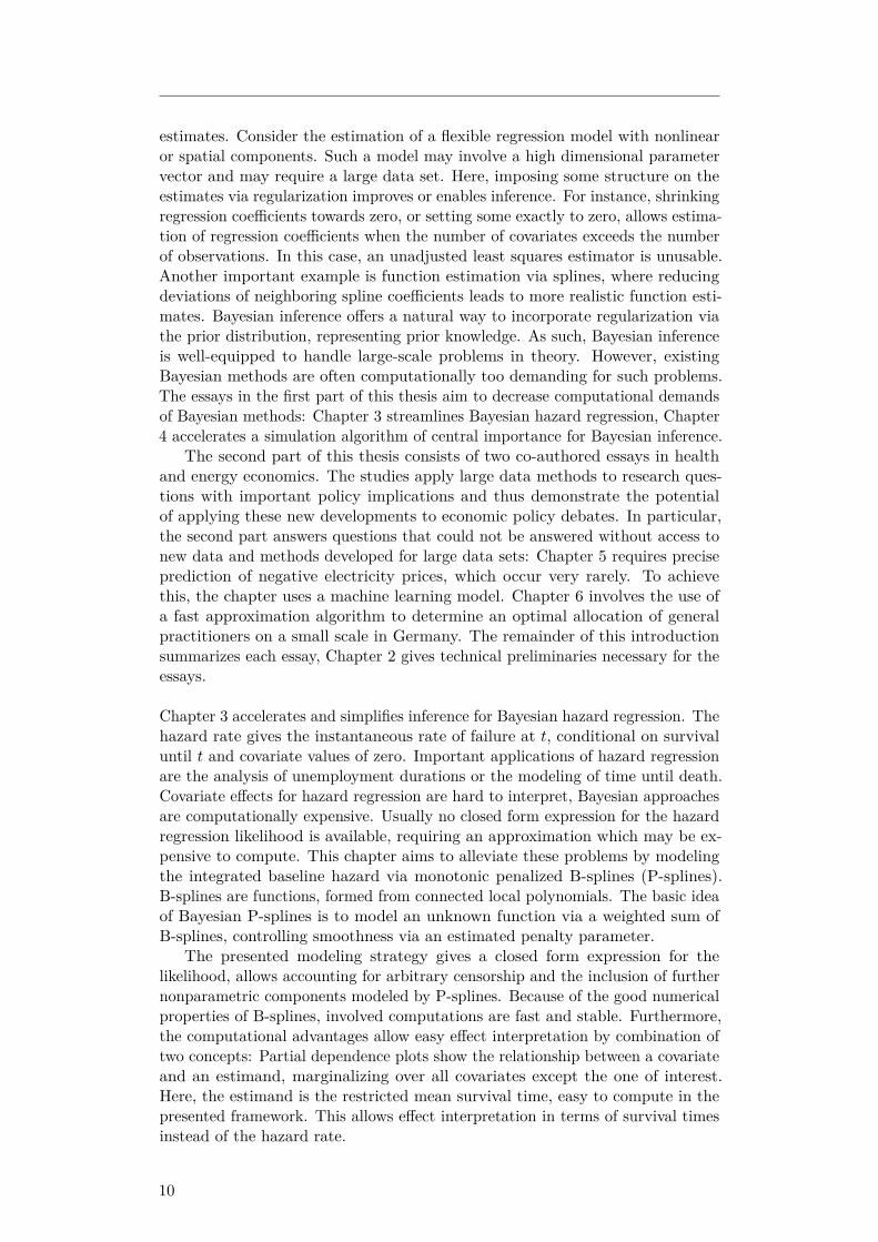
Figure 3.1: A: B-splines for varying order. Dashed, vertical lines mark the knots.B: Function obtained by weighted sum of B-splines. The red line is the estimatedfunction, given by the sum of the scaled basis functions below, here giving amonotone estimate.
with Jr = m+ lr − 2 andwr,j := x− kr,j
(lr − 1)h,
where h is the spacing between the knots. If function specific domain knowledgeis available for function fr, it can be used to set lr, i.e., if one function is known tobe a step function. Otherwise, one usually sets lr to the smallest value where thesmoothness of the estimated function is satisfactory, a good default is lr = 4 forr = 0, . . . , R. Define the design matrix Br ∈ RN×J with i, jth element Br,j(vi,r).Then we can write each vector of function evaluation as fr = Brβr and representthe linear predictor vector ξ compactly as
ξ = Zα+R∑r=0
Brβr.
Because B-splines vanish outside a domain spanned by lr− 1 + 2 knots (see figure3.1), the matrices B0, . . . ,BR are sparse. Hence the computation of the linearpredictor vector ξ is fast.
3.2.1 Priors
The flexibility of the B-splines basis increases with m, the number of knots, whichdetermines Jr, the number of basis functions for function fr. For a large numberof knots, the B-spline fit approaches a rough interpolation of the data whichis usually undesired behaviour. Varying m on the fly changes the number ofparameters, complicating inference. Using penalization, one can use fixed, largem, say m = 30 (so that we obtain a flexible fit) and control the smoothness of theestimated function by a single parameter penalizing unsmooth function estimates.See figure 3.2 for a demonstration. In a Bayesian context, this is handled bythe prior distribution of β0, . . . ,βR and the associated penalty parameters. As aresult, we can directly obtain precision measures for function estimates from the
22
3 Efficient Bayesian nonparametric hazard regression
1 2 3 4
23
0 1 2 3 0 1 2 3 0 1 2 3 0 1 2 3
−0.4
0.0
0.4
0.8
1.2
−0.4
0.0
0.4
0.8
1.2
z
y
penalty 0 1.5 1e+06
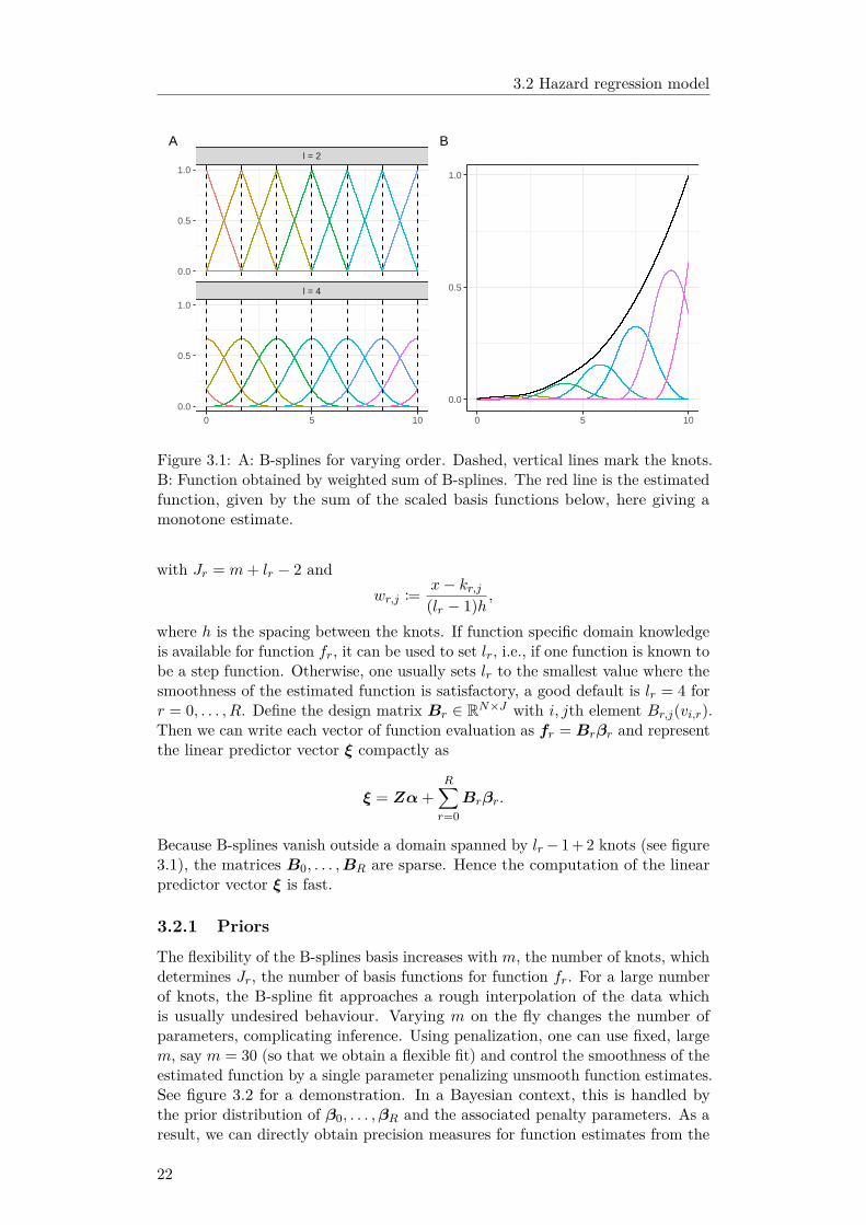
Figure 3.2: Influence of order l, difference order d and penalty parameter onfunction estimates. Data is simulated via yi ∼ N(sin(zi) log(zi + 0.5), 0.152).Rows are varying values of d, columns are varying values of l. Lines are theestimated function under varying penalty parameter. Without a penalty, theestimated function is very unsmooth, for a large penalty the function estimateapproaches a polynomial of degree d− 1.
posterior distribution. Furthermore, inference is automatic, in the sense that nopost-processing such as cross validation is necessary. Let ∆d be the differenceoperator of order d, defined recursively by
∆1βr,j := βr,j − βr,j−1,
∆d := ∆1∆d−1 for d > 1.
The curve fitting literature uses the squared dth derivative of the estimatedfunction as smoothness penalty. Eilers and Marx (1996) show that
λr
J∑j=d
(∆dβr,j)2, (3.1)
approximates this smoothness penalty. As such, λr controls the smoothness ofthe estimated function fr. For λr → ∞ the estimated function approaches apolynomial of degree d− 1. Increasing d results in smoother estimates. A valueof d > 3 is rarely used. We use d = 3 as default option and assume that d isthe same for β0, . . . ,βR. We use the prior distribution from Lang and Brezger(2004), who base their prior on (3.1). Here
∆dβr,j ∼ N(0, τ2r ) for j > d,
so that for instance
βr,j = βr,j−1 + er,j , for a difference of order d = 1,βr,j = 2βr,j−1 − βr,j−2 + er,j for a difference of order d = 2,βr,j = 3βr,j−1 − 3βr,j−2 + βr,j−3 + er,j for a difference of order d = 3.
23

3.2 Hazard regression model
with er,j ∼ N(0, τ2r ) for j = d, . . . , Jr. A high standard deviation τr, indicating an
unsmooth function, is associated with a low λr. Parameters β0,1, . . . , β0,d, β1,1, . . . ,β1,d . . . βR,d are assigned a flat prior p(·) ∝ 1. Let Dd
r ∈ R(Jr−d)×Jr denote amatrix representation of the difference operator for function fr. Then, element jof Dd
rβr is ∆dβr,j and
β>r Kdβr =Jr∑
j=d+1(∆dβr,j)2,
where Kd = D>d Dd is the penalty matrix. For instance, for d = 2, we have
D2 =
1 −2 1
1 −2 1. . . . . . . . .
1 −2 1
.
and
K2 =
1 −2 1−2 5 −4 1
1 −4 6 −4 1. . . . . . . . . . . . . . .
1 −4 6 −4 11 −4 5 −2
1 −2 1
.
We can write the prior for βr as
p(βr|τr) ∝ exp(− 12τ2r
β>r Kdβr), for r = 1, . . . , R. (3.2)
Because Kd is a sparse band matrix with range d + 1, we can exploit sparsematrix operations to compute the quadratic form β>r Kdβr in (3.2).
Some adjustments are necessary for modeling the log-cumulative baselinehazard f0 via P-splines. Because the cumulative baseline hazard is defined on[0, ti], the knot vector is a sequence from 0 to the largest t+i <∞. To achieve amonotonic function estimate for the log-cumulative baseline hazard3, we restrictthe prior (3.2) to non-decreasing vectors, resultant in a monotonic functionestimate as Brezger and Steiner (2008) show:
p0(β0|τ0) = p(β0|τ0)I[β0,1 ≤ β0,2 ≤ · · · ≤ β0,J0 ]. (3.3)
We can extend this to further nonlinear effects if a monotonic function estimate forf1, . . . , fR is desired. We assign a flat prior to regression coefficients α associatedwith linear effects. For positive scale parameters such as τr, a popular4 choice isan inverted gamma prior, see for instance Hennerfeind, Brezger, and Fahrmeir(2006) or Kneib and Fahrmeir (2007). We follow Gelman (2006), who recommendsa half Cauchy prior instead:
p(τr|φr) ∝ I[τr > 0](1 + (τr/φr)2)−1 for r = 0, . . . , R,3One might also model the cumulative baseline hazard, this involves an additional positivity
restriction on β0. We tried this but the Hamiltonian Monte Carlo sampler converged slowly.4The popularity of the inverted gamma prior is probably due to its convenience under a
Gaussian model, so that it has become somewhat of a default.
24

3 Efficient Bayesian nonparametric hazard regression
0.00
0.25
0.50
0.75
1.00
0 2 4 6τ
dens
ity
Figure 3.3: Half-Cauchy prior for τr with φr = 1.
with low scale parameter φr = 1 as default option. This puts most prior mass onsmooth functions, i.e., those with low τr. Due to the heavy tails of the Cauchydistribution, τr may be large, resultant in less smooth function estimates if thedata demands it. We estimate τr from the data, so that the parameter adjusts tothe number of B-splines.
3.2.2 Likelihood construction
We use P-splines to model the log-cumulative baseline hazard, so that
logH0(t) = f0(t) =J0∑j=1
β0,jB0,j(t) and
h0(t) = dH0(t)dt
= exp(f0(t)
)df0(t)/dt.
Because the derivative of a weighted sum of B-splines is
d∑Jrj=1 βr,jB
lrr,j(v)
dv= h−1
Jr∑j=2
Blr−1r,j (v)∆1βr,j , (3.4)
the baseline hazard is analytically available, resulting in a tractable likelihood. Be-cause the computation of (3.4) involves lower order B-splines, the computationaladvantages of B-splines carry over to the computation of the baseline hazard. Thelikelihood is L(θ|D) = ∏N
i=1 Li, with likelihood contributions L1, . . . , LN account-ing for censoring. Each likelihood contribution is the probability P (ti ∈ yi|ξi),except for uncensored survival times. Here the likelihood contribution is thedensity h(ti|ξi)S(ti|ξi), so that:
Li =
S(t−i |ξi)− S(t+i |ξi) if ti is interval censored,1− S(t+i |ξi) if ti is left censored,S(t−i |ξi) if ti is right censored,h(ti|ξi)S(ti|ξi) if ti is uncensored.
We need to compute the log-likelihood L for model evaluation and to samplefrom the posterior distribution via Hamiltonian Monte Carlo. There are someconvenient shortcuts for the computation of L. Let S denote the set of alluncensored observations. Define the vectors of totals zS := ∑
i∈S zi and bSj :=∑i∈S br(vi,r), which we have to compute only once. Then we can write the
log-likelihood for the uncensored observations as the sum ξS +∑i∈S ηi, where
ξS := α>zS +R∑r=0
β>r bSr (3.5)
25

3.3 Inference
is the sum of the linear predictor vector and ηi is defined as
ηi := log(df0(ti)dti
)− exp(ξi).
The computational cost of ξS does not grow with the cardinality of S. However,this does not hold for the computation of ∑ ηi, but computation of ξi is fastdue to the sparsity of the involved vectors. This applies to the contributionsof censored observations as well: Here, the likelihood contributions depend onthe value of the linear predictor, with aforementioned computational advantages.For instance, the likelihood contribution is log
(S(t−i |ξi)
)= − exp(ξi) for a right
censored survival time.
3.3 Inference
We use the probabilistic programming language Stan (Carpenter, Gelman, Hoff-man, Lee, Goodrich, Betancourt, Brubaker, Guo, Li, & Riddell, 2017) to samplefrom the posterior distribution
p(θ|D) = L(θ|D)p0(β0|τ0)R∏r=1
p(βr|τr)p(τr|φr). (3.6)
For point estimation we use the posterior mean, for interval estimation we use the0.025 and 0.975 quantile. A nice feature of simulation based Bayesian inferenceis the option to obtain uncertainty measures directly for functions of parametersfrom the samples of the parameters, e.g. for exp(f0) = H0.
Stan implements the No-U-Turn sampler for Hamiltonian Monte Carlo (Hoff-man & Gelman, 2014). This sampler converges quickly for high dimensionalposterior distribution of correlated parameters as for the problem at hand. It isalmost fully automatic5 and allows easy use of non-conjugate prior distributionssuch as the Cauchy prior for τr, unlike a Gibbs sampler. Furthermore, Stansupports sparse matrix operations6.
For models with nonparametric components the means of the functionf0, . . . , fr are not identified. For instance
ξi = f0(ti) + f1(v1,i)
is equivalent toξ?i = f?0 (ti) + f?1 (v1,i)
with f?0 (ti) = f0(ti) + c and f?1 (v1,i) = f1(v1,i)− c, so that the mean of f0 and f1is not identifiable. As such, we need to impose constraints or the sampler wouldnot converge. To that end, we use the decomposition from Kneib and Fahrmeir(2007) of the P-spline regression coefficients into a unpenalized and a penalizedpart:
βr = Urβur + Prβpr , for r = 1 . . . , R,
5There are some tuning parameters, but the sampler worked fine with default values exceptthe targeted acceptance rate, which we set to 0.99. This increases the effective sample size periteration for the cost of increased time per iteration (Stan Development Team, 2021).
6Stan also includes optimizing routines based on the automatic differentiation, so thatthe posterior mode (equivalent to penalized maximum likelihood) is also an option for pointestimation, for example for frequentist inference.
26

3 Efficient Bayesian nonparametric hazard regression
with priors p(βur ) ∝ 1 and βpr ∼ N(0, τ2r ). The matrix Ur contains the basis for
the null space of Kr, so that
(Urβur )>Kr(Urβur ) = 0.
As such, βpr captures the unpenalized polynomial of degree d− 1 in fr, see figure3.2 for an illustration. For the penalized part, it holds that
P>r KrPr = I,
where I denotes the identity matrix, resulting in a Gaussian prior for βpr . Pr canbe taken as Lr(L>r Lr)−1, where Lr comes from the factorized penalty matrixKr = LrL
>r . The first column of Pr is a vector of ones, so that the parameter βur,1
represents the mean of fr. Then, the estimate for fr is constrained by deleting thefirst column of Pr, which has a similar effects as imposing a zero mean constraint.We let the log-cumulative baseline hazard f0 sets the global mean, so that wecan sample β0 without further restrictions. The vector βpr is equivalent to avector of random effects, allowing the use of specialized Stan routines such as thenon-centered parameterization.
3.3.1 Model choice
Model choice in a Bayesian framework is an ongoing research area with severalcompeting approaches. We use expected log predictive density criterion (hence-forth elpd), because it is a measure for the generalizability of a model to unknowndata, which is usually the pertinent task. Vehtari and Ojanen (2012) derive thecriterion in a Bayesian decision theoretic approach: Here we choose some modelM which maximizes an utility function of our choice. Using the log score resultsin the elpd:
elpdM :=∫π(y) log pM (y|x,D) dy,
wherepM (y|x,D) :=
∫pM (y|x,D,θ)pM (θ|D)dθ
is the posterior predictive distribution for a new observation y under model M ,with covariates x. π denotes the distribution associated with the unknown datagenerating process. Using leave-one-out cross-validation, an estimator for theelpd is given by:
elpdM = N−1N∑i=1
log pM (yi|xi,D−i), (3.7)
where D−i is the data without observation i. The elpd measures predictiveperformance of a model, it does not contain an explicit penalty for the numberof parameters, however this can be estimated as shown by Vehtari, Gelman,and Gabry (2017). They also show how to compute (3.7) efficiently via Paretosmoothed importance sampling. Their method bypasses the need to computeN models, instead using log-likelihood evaluations from a single MCMC run.Magnusson, Andersen, Jonasson, and Vehtari (2019) present a method to furtherspeed up computation for large data sets based on subsampling.
3.3.2 Covariate effects
Let σ denote the follow-up time and µ = µ(ξ) denote the conditional expectationE[T |ξ]. If σ and the sample size are large enough so that we can precisely
27

3.3 Inference
estimate the survival time where the baseline survivor function tends to zero, wecan estimate µ via the identity
µ =∫ ∞
0S(u|ξ)du. (3.8)
In practice, this is rarely the case so that estimating the integral in equation (3.8)necessitates extrapolation. The restricted mean survival time (rmst), defined as
µσ := E[min(T, σ)|ξ] =∫ σ
0S(u|ξ)du
is an alternative which avoids extrapolation beyond the follow up time andbypasses the need to interpret effects in terms of the hazard rate (Stensrud,Aalen, Aalen, & Valberg, 2018). Because researchers can interpret the restrictedmean survival time as the average survival time until σ, the rmst has attractedmuch attention as a measure for covariate effects, see for instance Chen andTsiatis (2001), Royston and Parmar (2011) and Zhao, Tian, Uno, Solomon, Pfeffer,Schindler, and Wei (2012). We use numerical integration with the trapezoid ruleto estimate the integral in (3.8), where we split up the integral at min(t−1 , . . . , t−N ),to avoid extrapolation7:
µσ(ξ) = t?12 (1 + S(t1|ξ) + h
2 (S(t1|ξ) + S(σ|ξ)) + hK−1∑k=2
(S(t?k|ξ) + S(t?k+1|ξ)
),
with spacing h = σ/(K−1) and K control points t?k = min(t−1 , . . . , t−N )+(k−1)h.We can estimate the restricted mean survival time of one observation via
µσ(ξi) = Q−1Q∑q=1
µσ(ξqi ),
where the superscript q = 1 . . . Q denotes the qth draw from the posteriordistribution.
The most important application of the restricted survival time is the estimationof a binary treatment effect, the comparison between outcomes µσ1 (treatment)and µσ0 (control). Most commonly this is the simple difference µσ1 − µσ0 . However,inference for other forms such as ratios can easily be done in a Bayesian framework(Imbens & Rubin, 2015). A unit level treatment effect Wi is the comparison of µσ1and µσ0 for unit i. We estimate Wi via Wi = Q−1∑Q
q=1Wqi . An easy-to-interpret
scalar measure is the average treatment effect (ATE), which we estimate via
ATE = N−1N∑i=1
Wi.
We propose to combine partial dependence plots (Friedman, 2001) with therestricted mean survival to simplify effect interpretation for metric covariates:Say we are interested in the effect of the metric covariate vk. The basic ideaof partial dependence plots is to compute the restricted mean survival time,marginalizing over all parameters and covariates except vk. Let ξi denote thelinear predictor for unit i where we set the value of vik to vk. Then we create apartial dependence plot for the covariate vk by computing
(NQ)−1N∑i=1
Q∑q=1
µσ(ξqi )
7This might be problematic if the observed minimum is large. In this case extrapolating H0or log H0 might be preferable.
28

3 Efficient Bayesian nonparametric hazard regression
0
20
40
60
80
0.0 0.5 1.0 1.5 2.0survival time
base
line
haza
rd
A
f1
f2−1.0
−0.5
0.0
0.5
1.0
0.00 0.25 0.50 0.75 1.00v
f(v)
B
Figure 3.4: Functions involved in the simulation study. A: Additive Weibullbaseline hazard. B: Functions f1 and f2.
over a grid of control points vk,1, . . . , vk,C , plotting the result with the associatedposterior interval. We can do this for variables which we model by a linear or anonlinear component. Partial dependence plots may also be used for non-metricvariables.
A related concept is the marginal survival function. Often one is interested ina global average of the survival function. For the Cox model, a simple solution isthe baseline survival function, which is the survival function conditional on allcovariates taking the value zero. However, this might be nonsensical or requirean unwanted transformation of the covariates to achieve interpretability. Themarginal survival function allows averaging over the covariates and parameters.We compute it via
Saverage(t) = (NQ)−1N∑i=1
Q∑q=1
S(t|ξqi ).
We can furthermore condition on specific covariates values, for instance a subgroupindicator for group differences.
For longer chain lengths, one may use thinning to speed up computations,i.e., the use of every nth sample from the posterior distribution.
3.4 Simulation study
We investigate the performance of the presented methods under varying censoringmechanisms and sample sizes. For each censoring mechanism, we simulate 50data sets each with sample size N = 100, 200, 500, 1000, 2000. Survival times areadditive Weibull distributed with hazard where
h(ti|xi,α) = h0(ti) exp(z>i α+ f1(v1i) + f2(v2i)),h0(ti) = t5i + 2
√ti,
f1(vi1) = sin(4vi1) and f2(vi2) = 0.5[cos(5vi2)− 1.5vi2].
Figure 3.4 shows the baseline hazard and involved functions. The baselinehazard is bathtub shaped, exemplifying a shape that is hard to capture bycommon parametric methods yet highly relevant in practice. An example forsuch a mechanism is human mortality: here the hazard rate is high immediatelyafter birth, followed by a period with low hazard, while rising in later years.
29

3.4 Simulation study
100 200 500 1000 2000
f1f2
log cum hazard
0.00 0.25 0.50 0.75 1.000.00 0.25 0.50 0.75 1.000.00 0.25 0.50 0.75 1.000.00 0.25 0.50 0.75 1.000.00 0.25 0.50 0.75 1.00
−1
0
1
−1
0
1
−2
0
2
censoring none interval left low left high right low right high
Figure 3.5: Representative examples by sample size (columns), variable (rows).The color of the lines is mapped to the combination of the type of censoring withthe fraction of censored survival times. For instance, right low means 20% of thesurvival times are right censored. The x-axis is scaled to the interval [0, 1] forvisualization purposes. Each example is chosen to be closest to the overall meansquared error over all iterations.
Regression coefficients α are equally spaced between −0.3 and 0.3, covariatesz1, . . . , z5 are standard normal, v1 and v2 are standard uniform. There are fourvariants regarding the fraction of censored observations: no censoring, low (20%)and high (40%) percent censored observations for all three censoring types, and100% for interval censored. For all censoring types, we draw a simple randomsample of the failure times and censor afterwards.
To evaluate estimates, we compute the mse of f0, f1 and f2 on a grid of Ccontrol points er,1, . . . , er,C as
mse(f qr ) = C−1C∑c=1
(f qr (er,c)− fr(er,c)
)2
and the mse for α as
mse(αq) = 5−1(αq −α)>(αq −α).
Figure 3.5 shows representative examples of estimates, figure 3.6 shows the resultsfor the log mean squared error, henceforth log-mse. As might be expected for acomplex model, estimates for f0, f1 and f2 are quite imprecise for small samplesizes (N ≤ 200). The log-mse decreases with increasing sample size. For theestimation of α, f0 and f1 the censoring mechanism does not seem to cause largedifferences. However, the log-mse is usually highest under a high fraction of rightcensored observations and lowest under no censoring and interval censoring. Forestimation of the log-cumulative baseline hazard, there is a clear negative effect
30

3 Efficient Bayesian nonparametric hazard regression
●
●
●
●
●
●
●
●
●●● ●
●
●
●
●
●●
●●
●
●
●● ●
●
●●●
●●
●
●●
●
●
●●
●
●
●●
● ●
●●
●
●
●
●●
●
●●
●
●●
●●
●●
●
●
●●●
●
●
●●
●
●●
●
●●●
● ●
●●
●
● ●
●●
●
●●
100 200 500 1000 2000
alphaf1
f2log cum
hazard
none
inter
val
left lo
w
left h
igh
right
low
right
high
none
inter
val
left lo
w
left h
igh
right
low
right
high
none
inter
val
left lo
w
left h
igh
right
low
right
high
none
inter
val
left lo
w
left h
igh
right
low
right
high
none
inter
val
left lo
w
left h
igh
right
low
right
high
−3.5
−3.0
−2.5
−2.0
−1.5
−7.5
−5.0
−2.5
0.0
−7.5
−5.0
−2.5
0.0
−6
−4
−2
0
(log)
mse
censorship none interval left low left high right low right high
Figure 3.6: Boxplots showing log mean squared error by sample size (columns),variable (rows). The horizontal axis within each box corresponds to the combi-nation of the type of censoring with the fraction of censored survival times, forinstance right low means 20% of the survival times are right censored, which isfurthermore mapped to the color of each boxplot.
associated with the information loss from censoring. This effect is strongest forright censoring, where more information about the survival times is lost comparedto left- and interval-censoring, as the interval around the true survival time iswider. Under interval censoring, the log-mse for estimates of f0 is lowest forsmall sample sizes, however it does not improve much for N > 500. Overall, theestimation strategy works as desired, given a large enough sample size. However,large fractions of right censored observations may be problematic.
3.5 Application: Real estate data
The data set in this application consists of survival times of real estate ad-vertisements for flat rents. The advertisements were published on the websiteImmobilienScout24 in the year 2017. For a description of the data set and dataaccess see Boelmann and Schaffner (2018). The survival time is the number ofdays an advertisement is online. While there are several reasons why an adver-tisement may be taken offline, we assume that in the majority of cases someonerented the flat. To illustrate inference for a treatment effect, we estimate a hazardmodel for the city states Bremen and Hamburg, where we create a balanceddata set using coarsened exact matching (Iacus, King, & Porro, 2012). We chose
31

3.5 Application: Real estate data
Hamburg
Bremen
0.00
0.25
0.50
0.75
1 50 100day
stan
dard
ized
sur
viva
l fun
ctio
n
Figure 3.7: Standardized survival curves for Hamburg and Bremen with 0.025and 0.975 posterior quantile. Note that the posterior interval is very tight due tothe sample size and might be only visible when zooming into the figure.
Bremen and Hamburg because these are the only cities which are city statesthat are located within the same region (Northern Germany). There are 16480observations in Hamburg, of which 953 are right censored. In Bremen, the are7356 observations, of which 466 are right censored. We include several covariates
Table 3.1: Descriptive statistics
Mean Std. deviationVariable Bremen Hamburg Bremen Hamburgdays online (uncens.) 21.239 16.189 36.595 26.778days online (cens.) 42.790 23.939 89.599 45.876censoring indicator 0.063 0.058 0.244 0.233commission 0.018 0.023 0.132 0.151missing entries 5.232 4.130 2.432 2.098rent residual -0.480 1.443 1.942 2.494
in the model, see Table 3.1 for descriptive statistics: (1) The residual from ahedonic regression of rent price per square metre on a set of control variablessuch as age of the house. A positive residual indicates an overpriced flat. We usea similar set of variables as Eilers (2017), extending the model for the hedonicregression by a spatial effect. The residual then gives the relative price for a flatconditional covariates and the location. (2) The number of missing fields in theadvertisement. (3) Binary indicators for flats requiring a broker commission anda binary indicator for Hamburg, representing a treatment effect in our analysis.We define the individual treatment Wi effect as difference between restrictedmean survival times with follow up time σ = 100 days.
Figure 3.7 shows the marginal survival function for Hamburg and Bremen,indicating that flats in Hamburg are rented out quicker than in Bremen. Figure3.8 shows the partial dependence plots. An overly high price is associated with anincrease in the restricted mean survival time. This effect is approximately linear.An increase in the number of missing entries is associated with a decrease inrestricted mean survival time. This might be due to advertisement for unattractiveflats, where the supplier hopes to increase attractiveness by providing more
32

3 Efficient Bayesian nonparametric hazard regression
commission Hamburg
no yes no yes
12.5
15.0
17.5
20.0rm
st
Amissing entries rent residual
0 2 4 6 8 10 −6−4−2 0 2 4 6 8 10
10
20
30
40
50
rmst
B
Figure 3.8: Partial dependence plots for restricted mean survival time, for σ = 100days, with 0.025 and 0.975 posterior quantiles. A: Partial dependence plots forbinary covariates. B: Metric covariates.
● ●
●
●
●
−1880
−1840
−1800
−1760
no co
varia
tes
com
miss
ion
Hambu
rg
f(# N
As)
f(ren
t res
idual)
estim
ated
elp
d
Figure 3.9: Estimated elpd for the chosen models. From left to right, the x-axis gives the element which is added to the model, starting with a modelwithout covariates, so that the second model for the cumulative baseline hazard isH0(t) exp(β1commission), the third model H0(t) exp(β1commission+β2Hamburg)and so forth.
information.For Hamburg, the estimated average treatment effect ATE is −8.62, probably
due to higher demand. The associated posterior interval is [−8.21,−7.77], so thatthe effect is precisely estimated. Requiring a broker commission is associatedwith an increase in restricted mean survival time by 2.45 days. Because the shareof advertisements requiring a broker commission in the data set is low (2.1 %),the associated posterior interval [1.03, 4.19] is much wider.
Figure 3.9 shows the estimated expected log predictive density values, workingup from a model containing no covariates. While the elpd does not contain anexplicit penalty term for the number of parameters, including another parametermay decrease the elpd. The effect of the covariates on the elpd varies stronglybetween the variables. However, the order of the covariates influences this effect.For instance, including the broker commission hardly increases the elpd comparedto the inclusion of the number of missing entries.
3.6 Conclusion
This paper presents an approach for fast Bayesian hazard regression using mono-tonic P-splines. Because involved quantities are analytically available and wecan exploit sparsity for the involved computations, this estimation strategy iscomputationally more efficient than existing approaches. We leverage this effi-
33

3.6 Conclusion
ciency to simplify effect interpretation by combining partial dependence plotswith the restricted mean survival time approach. We tested the proposed strategywith numerical examples: Simulations show that the approach works well, anapplication shows that the approach gives useful results for a large data set.
There are several extensions of this work. It might be fruitful to relax theproportional hazards assumption. This may be done by allowing interactionswith survival or by allowing the baseline hazard to vary by subgroup. Whileusing P-splines for f1, . . . , fR is one (very good) choice among many, we arguethat monotonic P-splines are useful for logH0. For instance, one might use aGaussian process instead, which would be feasible in our framework.
34

Chapter 4
Fast, approximate MCMC forBayesian analysis of large datasets: A design based approach1
Abstract
We propose a fast approximate Metropolis-Hastings algorithm for large data setsembedded in a design based approach. Here, the loglikelihood ratios involved inthe Metropolis-Hastings acceptance step are considered as data. The buildingblock is one single subsample from the complete data set, so that the necessityto store the complete data set is bypassed. The subsample is taken via thecube method, a balanced sampling design, which is defined by the property thatthe sample mean of some auxiliary variables is close to the sample mean of thecomplete data set. We develop several computationally and statistically efficientestimators for the Metropolis-Hastings acceptance probability. Our simulationstudies show that the approach works well and can lead to results which are closeto the use of the complete data set, while being much faster. The methods areapplied on a large data set consisting of all German diesel prices for the firstquarter of 2015.
Keywords: Bayesian inference; Big Data; Approximate MCMC; Survey sampling
1This chapter has been published as: Kaeding, M. (2016). Fast, approximate MCMC forBayesian analysis of large data sets: A design based approach. Ruhr Economic Papers, 660,1–23. doi:10.4419/86788766
35

4.1 Introduction
4.1 Introduction
Consider the update step in the Metropolis-Hastings algorithm for the simulationof the posterior distribution
π(θ|D) ∝ L(θ|D)π(θ),
where θ is the parameter vector, π(θ) is the prior, D is the available data and Lis the likelihood
L(θ|D) =N∏k=1L(θ|Dk).
We restrict attention to the case where the observations are independent givenθ, most common under a regression framework. The update step consists ofthe following steps: Given the current value θc, a proposal θ? is drawn fromthe proposal distribution G(·|θc). The current value is set to the proposal withprobability
α(θc,θ?) = 1 ∧ L(θ?|D)π(θ?)G(θc|θ?)L(θc|D)π(θc)G(θ?|θc) . (4.1)
The computational cost for the computation of α = α(θc,θ?) is linear in N . As aresult, large data sets pose a problem for the algorithm. Due to the onset of largedata sets, accelerating the algorithm is a highly relevant issue (Green, Latuszynski,Pereyra, & Robert, 2015). The aim of this paper is to accelerate the update stepby using a computationally efficient and precise design based estimator for αusing a single fixed subsample of the data. Compared to repeatedly subsamplingthe data, this approach avoids two types of overhead: (1) Subsampling the data,(2) storing and accessing the data. This is especially relevant for data sets whichare too large to be read in memory.
Several proposals have been made to accelerate the algorithm by drawing asubsample for every update step: Korattikara, Chen, and Welling (2014) andBardenet, Doucet, and Holmes (2014) represent the update step as a hypothesistest. Maclaurin and Adams (2014) use a completion of the posterior distributionvia auxiliary variables. For their approach, a computationally cheap lower boundmust be available for all likelihood contributions. Quiroz, Kohn, Villani, andTran (2019) use a pseudo-marginal argument where an unbiased estimator for thelikelihood is needed: They construct this estimator by debiasing an exponentiatedestimator for the loglikelihood, relying on a normality assumption. To the best ofour knowledge, Maire, Friel, and Alquier (2015) is the only article considering theuse of subsamples which stay fixed during several iterations. Bardenet, Doucet,and Holmes (2017) provide a good overview over existing approaches.
We take the same perspective as these authors: Our algorithm belongs to theclass of noisy Monte Carlo algorithms: Here, we obtain deviates from a (close)approximation to the posterior distribution using the complete data set.
The paper is structured as follows: Section 2 gives background on noisyMCMC, Section 3 on sampling theory. Section 4 describes the proposed algorithm,Section 5 reports a simulation study. Section 6 applies the methods to a largedata set on gas prices. Section 7 concludes with a discussion.
4.2 Noisy Metropolis-Hastings
It is convenient to use the following representation of the update step of theMetropolis-Hastings algorithm, used by Korattikara, Chen, and Welling (2014)
36

4 Fast, approximate MCMC for Bayesian analysis of large data sets: A designbased approach
Algorithm 1 Metropolis Hastings update step for posterior simulationDraw u from U(0, 1)Set ρ to log[uπ(θc)G(θ?|θc)
π(θ?)G(θc|θ?) ]if ρ > φ then
Set θc to θ?end ifreturn θc
Algorithm 2 Metropolis Hastings algorithm for posterior simulation, genericversion
for r = 1 to R− 1 doDraw θ? from G(·|θc)Set φ to ∑N
i=1 Li(θ?|Di)− Li(θc|Di)Do Metropolis-Hastings update step for posterior simulation, using θ?, φSet θ(r) to θc
end forreturn θ(0), . . . ,θ(R−1)
and Bardenet, Doucet, and Holmes (2014): Draw θ? ∼ G(·|θc), u ∼ Unif(0, 1),and accept the proposal if
log[uπ(θc)G(θ?|θc)π(θ?)G(θc|θ?)
]< φ, (4.2)
where φ = ∑Nk=1 φk, is the sum of loglikelihood ratios:
φk = φ(θ?,θc|Dk) = logL(θ?|Dk)− logL(θc|Dk).
The MH algorithm simulates a Markov chain with transition kernel K whichis invariant under π(θ|D). Replacing the left hand side or the right hand sidein (4.2) by an estimator implies the use of an approximate transition kernel Kwhich in general is not invariant under π(θ|D). One exception is given by thepseudo-marginal approach by Andrieu and Roberts (2009), where an unbiasedestimator of the likelihood is available, used by Quiroz, Kohn, Villani, and Tran(2019). However, getting an unbiased estimator of the likelihood in a fixedsubsample context is not feasible without questionable assumptions and mightlead to trading small bias with high variance.
Although the theoretical properties of noisy MCMC are not completelyunderstood, there are some encouraging results: Alquier, Friel, Everitt, andBoland (2014) have shown that the stationary distribution of the Markov chainobtained using an estimator α = α(θc,θ?) for α is a useful approximation toπ(θ|D), provided that |α− α| is bounded. Nicholls, Fox, and Watt (2012) showthat, if a Gaussian unbiased estimator for log π(θ?|D)− log π(θc|D) with knownvariance is available, the update step of the Metropolis-Hastings algorithm canbe adjusted via a method called the penalty method, so that the chain targetsπ(θ|D) as desired. Usually, such an estimator is not available. Nicholls, Fox, andWatt (2012) show that plugging an estimate of log π(θ?|D)− log π(θc|D) into αleads to a chain which is very close to the penalty method, provided that theexpected absolute error E|α− α| is small. As such, the main objective here is tofind a computationally cheap estimator for φ, so that |α− α| is small.
37

4.3 Some sampling theory
4.3 Some sampling theory
Let U = {1, . . . , N} be a set of labels associated with a finite population of Nunits, here given by the complete data set. The aim of survey-sampling is toestimate a finite population total, y = ∑
k∈U yk of a variable y, using a sampleS ⊆ U . Totals are denoted by dots. The set S is selected via a stochastic selectionscheme, called the sampling design. Design based sampling is used when thecost of obtaining the value yk for all units k ∈ U is too expensive, so the samplesize n ..= |S| is usually much smaller than N . For this article, cost is given bycomputation time. In a design based approach, all randomization is due to thesampling design, while the values y1, . . . , yN of the study variable are unknownconstants.
A sample can be represented by a random vector
i = (i1, . . . , ik, . . . , iN )>,
where ik takes the value 1 if unit k is in the sample S and 0 otherwise. Thesampling design f(·) is a probability distribution on a support Q. Here, attentionis restricted to without-replacement sampling designs with fixed sample size, sothat
Q ={i ∈ {0, 1}N |
∑k∈U
ik = n}.
It holds thatEf [i] =
∑i∈Q
if(i) =.. η,
where the inclusion probability P (k ∈ S) = Ef [ik] = P (ik = 1) of an elementk is given by ηk. Note that the empty sample i = (0, . . . , 0)> and the censusi = (1, . . . , 1)> are in Q, corresponding to the cases n = 0 and n = N . For moreon sampling theory see Tille (2006) or Sarndal, Swensson, and Wretman (2003).
4.3.1 Sampling design: Cube sampling
Denoting sums of the form ∑k∈S k as ∑S k, the benchmark estimator for a total
y is the Horvitz-Thompson estimator:
ˆyHT =∑U
ikykηk
=∑Sykdk,
where dk = 1/ηk is called the design weight. Here, only sampling designs areused where all inclusion probabilities are equal, so that without loss of generalityηk = n/N for k ∈ U and
ˆyHT = N
n
∑Syk = Ny,
where y is the sample mean of y.The variance of the Horwitz-Thompson estimator can be lowered by exploiting
additional information: Assume zq,k, q ∈ {cube, greg} is known for all elementsin the population, where zq,k = (zq,k,1, . . . , zq,k,pq )> is a vector of values ofpq auxiliary variables for unit k. The auxiliary variables zcube,1, . . . , zcube,pcube
and zgreg,1, . . . , zgreg,pgreg may intersect and may be identical or distinct. Letzcube = ∑
U zcube,k denote the known total of the auxiliary variables used for cube
38

4 Fast, approximate MCMC for Bayesian analysis of large data sets: A designbased approach
(0,0,0)
(0,0,1)
(0,1,0)
(0,1,1)
(1,0,0)
(1,0,1)
(1,1,0)
(1,1,1)
A
(0,0,0)
(0,0,1)
(0,1,0)
(0,1,1)
(1,0,0)
(1,0,1)
(1,1,0)
(1,1,1)
B
Figure 4.1: A: Set of all samples as represented as cube, for the case N = 3,giving 23 = 8 possible samples. B: Set of all samples with constraint space. Inthis case, there are no samples in the constraint space.
sampling. The objective of balanced sampling is to obtain a sample, respectingthe vector of inclusion probabilities η, so that the constraint
ˆzHTcube = zcube (4.3)
holds. For equal inclusion probability designs as used here, this is equivalent tothe constraint
n−1∑Szcube,k = N−1∑
Uzcube,k,
so that the sample mean of the auxiliary variables used for cube sampling isequal to their population mean. Usually, an exact solution is not possible for allauxiliary variables, so that samples are found which satisfy (4.3) approximately.Here, the role of the balanced sampling algorithm is to find a sample which is“close” to the complete data set. The choice of auxiliary variables is discussed insection 4.4. We will use the cube method Deville and Tille (2004), which is basedon a geometrical representation of a sampling design: Let C = [0, 1]N denote acube equipped with 2N vertices. C represents the set of all 2N possible samplesfrom a population of size N , where every vertex of C is associated with a sample,see figure 4.1.
Define the vector ak := zcube,k/ηk and the pcube ×N matrix
A := (a1, ..,ak, . . . ,aN ),
then the balancing equations (4.3) can be written as
Ai = Aη. (4.4)
The system of equations (4.4) defines the hyperplane
P = η +K(A)
in RN , where K(A) is the kernel of A. The basic idea of cube sampling is tochoose a sample as a vertex of C in P or, if that is not possible, near P. Cubesampling consists of two phases: The flight phase is a martingale with initial
39

4.3 Some sampling theory
value η in the constraint space K = C ∩ P , where the constraint (4.3) is satisfied.At the end of the flight phase a vector i? is obtained. If all elements of i? areeither 1 or 0, the landing phase is not necessary as a vertex of C is reached. Ifthis is not the case, the balancing equations are relaxed and the elements of i?are randomly rounded so that
E[i] = η,
hence, given inclusion probabilities are respected. Deville and Tille (2004)show that it is always possible to satisfy one balancing equation. It holds that∑U ηk = n. As such, setting zcube,1 = η guarantees a fixed sample size, as the
balancing equations are relaxed starting with the last auxiliary variable zcube,pcube.
The authors show that the cube method achieves the bound
|zcube,j − ˆzHTcube,j |N
= O(pcube/n), for j = 1, . . . , pcube, (4.5)
where f = O(g) if there is an upper bound of |f | which is proportional to g. Dueto the bound (4.5), the error becomes small if the sample size is large, comparedto the number of auxiliary variables. We will use the implementation by Chauvetand Tille (2006) with computational cost linear in N .
4.3.2 Regression estimator
The Horvitz-Thompson estimator is the only estimator which is unbiased for allsampling designs. However, there are better estimators in an MSE-sense if thiscondition is relaxed. A large class is given by the generalized regression estimator(greg). Model the study variable y via
yk = β>zgreg,k + εk, εk ∼ N(0, ω2).
The generalized regression estimator ˆygreg for a total y is given by the sum offitted values plus the Horvitz-Thompson estimator for the prediction error:
ˆygreg =∑Uyk + ˆeHT (4.6)
=β>zgreg + N
n
∑S
(yk − yk), (4.7)
where yk = z>k β is the fitted value of element k, β is
β =(∑Szgreg,kz
>greg,k
)−1∑Sykzgreg,k,
and ek is the residual ek = yk − yk. The generalized regression estimator can alsobe written as weighted sum ∑
S wkyk, where the weights
wk = N/n[1 + (N/n)(zgreg − ˆzHTgreg)>× (4.8)(∑
Szgreg,kz
>greg,k
)zgreg,k
], for k ∈ S,
depend on the sample but not on the study variable. Hence, the same weightvector can be used for several variables, so that the estimator is cheap to compute.The greg weights (4.8) satisfy the calibration equation
40

4 Fast, approximate MCMC for Bayesian analysis of large data sets: A designbased approach
Algorithm 3 Approximate Metropolis-Hastings - phase 1Select subsect S ⊂ U via cube method, using auxiliary variableszcube,1, ..., zcube,pcube
Set j to 1for r = 1 to pgreg × 100 do
Draw θ? from G(·|θc)Set φ to ∑S φkDo Metropolis-Hastings update step for posterior simulation, using θ?, φSet θ(r) to θcif r modulo 100 = 0 then
for k ∈ U doSet zgreg,k,j to φk
end forSet j to j + 1
end ifend for
Algorithm 4 Approximate Metropolis-Hastings - greg, basic versionDo approximate Metropolis-Hastings - phase 1for k ∈ S do
Compute wkend forfor r = 1 to R do
Draw θ? from G(·|θc)for k ∈ S do
Compute φkend forSet ˆφ to ∑S wkφkDo Metropolis-Hastings update step for posterior simulation, using θ?, ˆφSet θr to θc
end forreturn θ(0), . . . ,θ(R−1)
∑Swkzgreg,k = zgreg.
For equal inclusion probabilities, the approximate variance of the generalizedregression estimator is, up to a constant, given by the sum ∑
U(yi − z>greg,kb)2,where
b =(∑Uzgreg,kz
>greg,k
)−1∑Uykzgreg,k.
As such, predictive power for y is the main requirement for the auxiliary variables.
4.4 Description of algorithm
The objective is to estimate the total φ = ∑U φk. The basic idea is to combine
a sample obtained by cube-sampling with a regression estimator. Denote theposterior distribution associated with a subsample S by πS . The algorithmconsists of two phases. In the first phase, a sample is chosen via cube sampling,
41

4.4 Description of algorithm
Algorithm 5 Approximate Metropolis-Hastings - greg, ridge variantDo approximate Metropolis-Hastings - phase 1for r = 1 to R do
Draw θ? from G(·|θc)for k ∈ S do
Compute φkend forSet c to M>φfor i = 1 to pgreg doαi ← ci/λi
end forSet σ2 to (n− pgreg)−1(φ−Mα)>(φ−Mα)Set κ to pgregσ2
ξ>ξfor i = 1 to pgreg do
Set ξi(κ) to ci/(λi + κ)end forSet ˆφ to ξ(κ)> ˜zgreg + (N/n)
((∑S φk)− ξ(κ)> ˜zgreg,S
)Do Metropolis-Hastings update step for posterior simulation, using θ?, ˆφ
end forreturn θ(0), . . . ,θ(R−1)
so that the posterior distribution from this subsample is close to π. To find ameasure for closeness, the result of Maire, Friel, and Alquier (2015) is used. Theseauthors have shown that the minimal Kullback-Leibler distance from πS to πU isminimized if the sufficient statistics for θ in S are equal to the sufficient statisticsin the population. For many nontrivial cases, there exists no such sufficientstatistic which can also be written as sum (as would be necessary for the use ofcube sampling). However, the result serves as a general guide, in that statisticswhich summarize the complete data D set are used. Such statistics can be derivedfrom inspection of the posterior distribution. Note that the computation timeof cube sampling algorithm scales badly with the number of auxiliary variables,so that a low number of auxiliary variables for the cube sampling algorithm ispreferable. Also during the first phase, auxiliary variables for the regressionestimator are computed. A good predictor for the value of φ(θ?,θc|Dk) is givenby φ(·, ·|Dk), for arguments near θ? and θc. This is used to obtain the auxiliaryvariables for the regression estimator: If the subsample is obtained, the posteriordistribution πS is an overdispersed approximation to π so that the support ofθ is covered by πS . The auxiliary variables for the regression estimator aresubsequently computed as followed: A regular Metropolis-Hastings algorithmis run using the subsample for 100pcube iterations. Every 100th iteration, theloglikelihood ratio obtained from the current and proposed value of θ is used asauxiliary variables, so that the auxiliary variables are computed as
zgreg,k,j = φ(θ?,θ(r)|Dk),
for k ∈ S, r = 100, 200, . . . , 100pgreg, where j = r/100 varies with r.The complete data set only has to be available for the first phase. For
the second phase, the Metropolis-Hastings algorithm proceeds using the sub-sample with φ replaced by an estimator using the derived auxiliary variableszgreg,1, ..., zgreg,pgreg . We use the posterior mode from the trial run of the firstphase as starting values.
42

4 Fast, approximate MCMC for Bayesian analysis of large data sets: A designbased approach
4.4.1 Ridge variant
The greg estimator can be improved by optimizing the predictions for the valuesof φk. We use the ridge estimator to achieve better prediction performance. Thisestimator has the following advantages: (1) It is available in closed form2, as
β(κ) =(∑Szgreg,kz
>greg,k + Iκ
)−1∑Sykzgreg,k.
(2) Shrinkage is controlled by a single parameter κ. (3) The complete dataposterior distribution is better covered with a higher number of auxiliary variables.This results in multicollinearity, as the auxiliary variables zgreg,1, ..., zgreg,pgreg arestrongly correlated, so that the matrix ∑S zgreg,kz>greg,k is ill conditioned for largepgreg. However, this is a desired property, as it indicates strong correlation withfuture values of φ(·, ·|Dk), k ∈ U . Hence, multicollinearity is a consequence of aset of useful auxiliary variables, which in turn is solved by the ridge estimator.
The third point suggests a simple heuristic to set pgreg: It is set at leastso large that the matrix ∑S zgreg,kz>greg,k is ill conditioned. Following Hoerl,Kannard, and Baldwin (1975), the shrinkage parameter κ is set as
κ := kσ2
β>β,
where σ2 is an estimate for var(φ|zgreg,1, ..., zgreg,pgreg ). While determining κ viacross validation might be preferable, using a closed form expression is much faster.In addition, cross-validation is used to estimate the out-of sample predictionerror. However, the procedure used here is based on the assumption that thesubsample is similar to the full data set. Given κ, the ridge variant of the gregestimator can be quickly computed using precomputed entities. For details seeappendix 4.A.
4.5 Simulation study
4.5.1 Setup
Here, results of a simulation study will be reported. The simulation was carriedout in R and C++ via the Rcpp interface (Eddelbuettel & Francois, 2011). Wegenerated M = 100 data sets from the model
yk = x>k β + εk, εk ∼ N (0, σ2), k = 1, . . . , N = 100000,
where x1 = (1, . . . , 1)> and the elements of x2, ...,x5 are draws from a uniformdistribution with minimum and maximum given by −2 and 2. The elementsof the parameter vector θ = (β>, log σ)> are deviates from a standard normaldistribution. The posterior distribution is simulated using the algorithm describedin section 4.4. We use a random walk Metropolis-Hastings sampler, where thevariance of the proposal distribution is scaled during burnin so that the acceptanceprobability is around 0.234. We use R = 100000 iterations, taking the first halfof the chain as burnin. For reference, we also simulate the posterior distributionusing the complete data set and use a variant where no auxiliary variables areused, so that φ is estimated via the sample mean. To study the gain of the cube
2Unlike e.g., the LASSO or the elastic net estimator, which might be preferable from aprediction perspective.
43

4.5 Simulation study
0 1 3 5 10 20 30
●
●
10
20
gaussian
ht GREG ridge GREG ridge GREG ridge GREG ridge ridge ridgetype_design
spee
dup
Figure 4.2: Speed up relative to the use of the complete data set for the gaussianlikelihood. Columns: Varying values of of pgreg.
sampling procedure, the sample was additionally chosen using simple randomsampling (srs); which is equivalent to cube sampling with a single auxiliaryvariable given by the inclusion probabilities. We use pgreg = 1, 3, 5, 10, 20, 30auxiliary variables for the regression estimator. For the basic greg estimator,it was not possible to set pgreg ≥ 20 due to multicollinearity. In addition, wegenerated data sets from the model yk ∼ Poisson(exp(x>k β)), with the sameconfigurations as above otherwise. For both models, the auxiliary variables usedfor cube sampling are derived from the likelihood: For the gaussian likelihood, wetake the residuals and the squared residuals obtained from the maximum likelihoodestimator βml = (X>X)−1X>y as zcube,1 and zcube,2. In addition, we generatethree draws from N(βml, 3σ2
mlX>X)−1), where σ2
ml = N−1∑U(yk − x>k βml)2
and use the associated residuals (and the squared residuals) as auxiliary variables.For the poisson likelihood, we use the loglikelihood kernel ykx>k β − exp(x>k β) asauxiliary variables. The maximum likelihood estimator is obtained via numericalmethods, otherwise values of β were obtained as above.
4.5.2 Results
The main criterion is the root mean squared error (rmse) for the true parametervector θ:
rmse(θ) =
√√√√16
6∑i=1
(θi − θi)2,
where θi is estimated using the posterior mean. We report the relative root meansquared error, in reference to the use of the complete data set: rmse(θ)/rmse(θU ),where rmse(θU ) is the rmse obtained by the use of the complete data set.Speedup: The speedup, defined as computation time using the given method,divided by the computation time using the complete data set, is shown in figure4.2. The basic greg variant is by far fastest, while the speedup for the ridgevariant drops for larger number of auxiliary variables.Parameter vector: Figure 4.3 shows the relative root mean squared error forthe true parameter vector θ. It can be seen that the error mainly depends onpgreg: If there are enough auxiliary variables for the estimation (in this case,around 20), the relative rmse can approach 1. This holds for both likelihoods.Cube sampling reduces the error, although the effect is larger for the gaussianlikelihood. We interpret this as a sign that the auxiliary variables are betterchosen for the gaussian likelihood. For a large number of auxiliary variables used
44

4 Fast, approximate MCMC for Bayesian analysis of large data sets: A designbased approach
0 1 3 5 10 20 30
gaussianpoisson
ht cu
beht
srs
GREG cube
GREG srs
ridge
cube
ridge
srs
GREG cube
GREG srs
ridge
cube
ridge
srs
GREG cube
GREG srs
ridge
cube
ridge
srs
GREG cube
GREG srs
ridge
cube
ridge
srs
ridge
cube
ridge
srs
ridge
cube
ridge
srs
0
4
8
12
0
4
8
12
estimator + sampling design
Rel
ativ
e ro
ot m
ean
squa
red
erro
r, lo
gsca
le
Design Cube sampling (cube) Simple random sampling (srs)
Figure 4.3: Root mean squared error for θ, relative to root mean squared errorobtained with complete data set, plotted on log scale for visualization. Rows:Gaussian and poisson likelihood. Columns: Varying values of of pgreg.
45
4.5 Simulation study
ridge, p=30
srs
ridge, p=3
cube
ridge, p=3
srs
ridge, p=30
cube
complete data set GREG, p=3
cube
GREG, p=3
srs
−0.48 −0.47
−0.48 −0.47 −0.48 −0.47
−0.50
−0.49
−0.48
−0.47
−0.46
−0.50
−0.49
−0.48
−0.47
−0.46
−0.50
−0.49
−0.48
−0.47
−0.46
true quantile
empi
rical
qua
ntile
Figure 4.4: Exemplary quantile-quantile plots for a single parameter.
46

4 Fast, approximate MCMC for Bayesian analysis of large data sets: A designbased approach
0 1 3 5 10 20 30
0.010.99
ht cu
be ht si
GREG cube
GREG si
ridge
cube
ridge
si
GREG cube
GREG si
ridge
cube
ridge
si
GREG cube
GREG si
ridge
cube
ridge
si
GREG cube
GREG si
ridge
cube
ridge
si
ridge
cube
ridge
si
ridge
cube
ridge
si
−5
0
5
10
−5
0
5
10
estimator + sampling design
Rel
ativ
e ro
ot m
ean
squa
red
erro
r, lo
gsca
le
Design cube si
Figure 4.5: Gaussian likelihood with known variance: Root mean squared errorfor quantiles of θ, relative to root mean squared error obtained with completedata set, for quantile q = 0.01, 0.99.
for estimation, this difference becomes small. Given a fixed value of pgreg, thedifference in error between the basic greg estimator and the ridge estimator aresmall. However, the ridge variant allows the use of a larger number of auxiliaryvariables and is therefore to be preferred.Quantiles: To study the accuracy of the simulated posterior distribution, weset σ equal to one and assume it to be known, so that the posterior distributionunder a non-informative prior β ∝ constant is given by a multivariate normaldistribution with variance Σ = (X>X)−1 and mean ΣX>y. As such, we canevaluate how well the true posterior distribution is simulated as whole, beyondpoint estimation. Exemplary quantile-quantile plots for a single parameter areshown in figure 4.4. The results are similar to the ones regarding θ: Moreauxiliary variables lead to a better approximation of the results of the completedata set, cube sampling improves over simple random sampling. Figure 4.5 showsthe relative root mean squared error for the marginal quantiles of θ1, . . . , θ5. Theroot mean squared error of the quantile vector is computed as:
rmse(Qq(θ)) =
√√√√15
5∑i=1
(Qq(θi)− Qq(θi))2,
for q = 0.01, 0.99, where Qq(x) is the q-Quantile of x. Here, the results are similarto the ones regarding θ as well, however the relative root mean squared errordoes not approach 1 as fast as for point estimation.
4.6 Application
The methods presented here will be applied on a large data set consisting of themost recent gas price for every hour for every gas station in Germany for thefirst quarter of 2015. The data set consists of 31 million rows. We estimate the
47

4.7 Discussion
●
●
●
●
●●●
●●
●
●
●
●
●
●
●
●
●
●●
●●●
● ●●●●
●●●
●
●
●
●
●
●
●
−6
−4
−2
0
01:0
002
:0003
:0004
:0005
:0006
:0007
:0008
:0009
:0010
:0011
:0012
:0013
:0014
:0015
:0016
:0017
:0018
:0019
:0020
:0021
:0022
:0023
:0024
:00ar
alav
iaes
so jet
nona
mesh
ell starm
ontueswed
thur
s fri satsu
n
Coefficient
Pric
e in
cen
t
Figure 4.6: Coefficient plot (posterior means). Reference categories are addedas red points. Posterior intervals for 0.01-quantile and 0.99-quantile are barelyvisible and omitted.
regression model:
pricei,t =β1 + fperiodic(weekday) + fperiodic(hour)+6∑j=2
βjI[brandi = j] + εi,t, εi,t ∼ N(0, σ2),
where the periodic effects are estimated using dummies, setting one categoryequal to zero, so that θ = (β1,β
>day,β
>hour,β
>brand, σ)>. We use the ridge variant
with a sample size of n = 10000 and pgreg = 50 auxiliary variables. For the cubesampling, 3 partial least squares latent variables are used. Partial least-squareslinear combinations are fast to compute, and summarize the design matrix whilepreserving the correlation with y. The algorithm takes about 11 minutes on aIntel xeon cpu e5 with 2.4GHZ. Figure 4.6 reports the estimated posterior meansof the regression coefficents. Most variation is explained by the hourly effects,diesel price is most expensive in the morning, least expensive in the eveningaround 19:00 with a difference of around 7 cents. The day of the week effect isvery small, compared to the hour effect: Gas prices are highest on mondays, withan estimated price difference of less than 0.5 cent. The most expensive brand isShell, followed by Aral. The smaller brands (Star and Jet) are more than 3 centscheaper than Aral. These results are country-wide and do not take local effectsinto account, mainly the effect of the location of the gas station. Furthermore,there might be an interaction between the day of the week and the hour of theday. These topics should be the subject of a separate study.
4.7 Discussion
We developed an approximate version of the Metropolis-Hastings using a singlesubsample. Our simulation study shows that the algorithm can produce posteriorsimulations which are almost identical to the use of the full data while being several
48

4 Fast, approximate MCMC for Bayesian analysis of large data sets: A designbased approach
orders of magnitudes faster. The methods were validated using a simulationcomparing the inferences obtained from the approximate posterior to the completedata posterior. The results suggest that the error obtained from using thealgorithm is small enough for practical purposes for standard models. However,further work regarding more complex models is necessary.
We propose to use this approximate version for the simulation of a posteriordistribution which is used directly for inference. However, there are furtherpossible applications for the algorithm; the algorithm might be used for the casewhen a fast approximation to the posterior distribution is of use, e.g., during theburnin of an adaptive Metropolis-Hastings algorithm.
49

4.A Appendix
4.A Appendix
Computation of Ridge estimator
For the modelφ = Zgregβ + e,
the ridge estimator for a given smoothing parameter κ is given by β = (Z>gregZgreg+κI)−1Zgregφ, where the rows of Zgreg are given by zgreg,k, for k ∈ S. DefineM ..= ZgregG, ξ ..= G>β, then
φ = ZgregGG>β + e = Mξ + e;
where Z>gregZgreg = GΛG> is the eigen-decomposition of Z>gregZgreg with or-thonormal G, i.e., G>G = GG> = I, so that Λ = diag(λ1, . . . , λk),
λ1 ≥ λ2,≥ · · · ≥ λp
where λ1, . . . , λp are the eigenvalues of Z>gregZgreg. It holds that Z>gregZgreg+cI =G(Λ + cI)G>, so that
(Z>gregZgreg + κI)−1 = G(Λ + κI)−1G>,
andβ(κ) = G(Λ + κI)−1M>φ→
ξ(κ) = (Λ + κI)−1M>φ.
Define c ..= M>φ. Than, the elements of ξ(κ) are
ξi = ciλi + κ
, i = 1, . . . , pgreg.
Following Hoerl, Kannard, and Baldwin (1975), the ridge parameter is set as:
κ = pgregσ2
ξ(0)>ξ(0). (4.9)
The residual variance is estimated using the usual unbiased estimator
σ2 = (n− pgreg)−1∑i∈S
(φi − z>i β(0))2
= (n− pgreg)−1(φ−Mξ(0))>(φ−Mξ(0)).
The vector β(κ) does not have be computed, using representation (4.7) of thegreg estimator: Define ˜zgreg := z>gregG and ˜zgreg,S := (∑S zi)>G, then φ isestimated via:
ξ(κ)> ˜zgreg + (N/n)(
(∑Sφk)− ξ(κ)> ˜zgreg,S
).
The vectors ˜zgreg and ˜zgreg,S only have to be computed once.
50

Part II
Applications in energy andhealth economics
51


Chapter 5
Market premia for renewablesin Germany: The effect onelectricity prices1
Abstract
Due to the growing share of “green” electricity generated by renewable energytechnologies, the frequency of negative price spikes has substantially increased inGermany. To reduce such events, in 2012, a market premium scheme (MPS) wasintroduced as an alternative to feed-in tariffs for the promotion of green electricity.Drawing on hourly day-ahead spot prices for the time period spanning 2009 to2016 and employing a nonparametric modeling strategy called Bayesian AdditiveRegression Trees, this paper empirically evaluates the efficacy of Germany’s MPS.Via counterfactual analyses, we demonstrate that the introduction of the MPSdecreased the number of hours with negative prices by some 70%.
Keywords: Negative electricity prices; Merit order effect; Bayesian AdditiveRegression Trees
1This paper is jointly written with Manuel Frondel and Stephan Sommer and has beenpublished as: Frondel, M. and Kaeding, M. and Sommer, S. (2020). Market premia forrenewables in Germany: The effect on electricity prices. SFB 823 Discussion paper, 13, 1–31.doi:10.2139/10.17877/DE290R-21016 and Frondel, M. and Kaeding, M. and Sommer, S. (2020).Market Market premia for renewables in Germany: The effect on electricity prices. USAEEWorking Paper, 456(20), 1–31. doi:10.2139/ssrn.3643762
53

5.1 Introduction
5.1 Introduction
Almost all over the world, policy-makers foster the deployment of renewableenergy technologies, such as solar and wind power, as a means to reduce carbonemissions. The European Union (EU), for instance, aims at raising the shareof “green” electricity, produced by renewable energy technologies, in electricityconsumption from about 29% in 2015 to 56% by 2030 (Agora, 2019). To achievethis target, the majority of Member States has established promotion schemesfor renewable energy sources (RES) that are based on subsidies (IEA & IRENA,2018).
In Germany, for example, since the beginning of the new millennium, greenelectricity has been promoted via technology-specific feed-in tariffs (FITs) thatguarantee fixed payments per kilowatthour (kWh) to the plant operators for upto 21 years. Moreover, grid operators are obliged to give priority dispatch toRES (Andor, Frondel, & Vance, 2017). In the aftermath of the introduction ofthe feed-in tariff system, Germany has been very successful in increasing REScapacities, yet their massive increase has come at high cost: Currently, the annualpromotion costs amount to more than 25 billion euros, equaling about 1% of theGerman GDP (Andor, Frondel, & Sommer, 2018).
In addition to the substantial cost due to the unconditonal payment offixed tariffs irrespective of demand levels, the steadily growing amount of greenelectricity has further adverse economic effects: it tends to increase both gridbalancing costs and the frequency of negative prices (Nicolosi, 2010; Weber, 2010).In fact, while RES plants are not obliged to contribute to grid stability, abundantgreen electricity production may lead to negative prices when a high electricitysupply coincides with a low demand, thereby inducing welfare losses (Andor,Flinkerbusch, Janssen, Liebau, & Wobben, 2010).
Gerster (2016), for instance, demonstrates that the growing feed-in of greenelectricity raises the probability of negative price spikes and thus threatens thefinancial viability of conventional plants. Negative prices primarily arise becauseconventional power plants face substantial ramp-up costs (Gerster, 2016) and,hence, are most often not shut down despite negative revenues due to negativeprices. Not least, numerous studies argue that there is a negative link betweengreen electricity generation and the wholesale price, commonly referred to as themerit-order effect (Cludius, Hermann, Matthes, & Graichen, 2014; de Lagarde &Lantz, 2018; Paschen, 2016; Praktiknjo & Erdmann, 2016; Wurzburg, Labandeira,& Linares, 2013).
To avoid such adverse effects and to align the production of green electricitywith market signals, many countries have implemented market premium schemesthat pay operators of renewable plants a variable bonus on top of the wholesaleelectricity price, rather than guaranteeing fixed feed-in-tariffs (RES, 2018). Ger-many, for example, introduced such a market premium scheme (MPS) in January2012 and revised it in August 2014.
Using hourly day-ahead spot prices for the time period spanning January 2009to December 2016, this paper empirically evaluates the efficacy of the GermanMPS, particularly with respect to reducing the frequency of negative price spikes.To this end, we employ a nonparametric modeling strategy called BayesianAdditive Regression Trees (BART), which is highly appropriate for identifyingnonlinear interactions between covariates (Hill, 2011) and for predicting thoseelectricity prices that would have emerged in the counterfactual scenario withoutthe MPS. Our results indicate that the BART method is very successful in
54

5 Market premia for renewables in Germany: The effect on electricity prices
replicating past electricity prices, as we are able to replicate those roughly 470hours in which negative prices occurred within the sample period of 2009 to 2016.
Moreover, our results suggest that the introduction of the MPS led to fewerhours with negative prices, particularly in the morning, and fewer positive pricepeaks relative to the counterfactual situation of an absent MPS. By comparisonwith this counterfactual, we demonstrate that negative electricity prices wereavoided by some 70%, in more than 560 hours. Based on these empirical results,we conclude that the MPS turned out to be effective in increasing the marketintegration of renewable energy technologies and, hence, in reducing the costs oftheir promotion.
The subsequent sections describe Germany’s electricity market and its MPS,as well as the data base underlying our research. Section 5.4 briefly introducesthe BART modeling method, while Section 5.5 presents our empirical results.The last section summarizes and concludes.
5.2 Germany’s Market Premium for RES
Germany stipulated ambitious targets for the expansion of RES, aiming atincreasing the share of RES-based electricity in consumption to 35% by 2020and to 80% by 2050. As more than 35% of electricity consumption was coveredby RES technologies in 2019, compared to less than 7% in 2000 (BMWi, 2017),Germany has already reached its 2020 target. Clearly, the key driver of this rapidexpansion is the Renewable Energy Sources Act (Erneuerbare-Energien-Gesetz,EEG), which came into force in 2000. Its key characteristic is a set of technology-specific FITs that are granted for up to 21 years in an intertemporally fixedamount. While exceeding the average generation cost of conventional electricity,in many cases substantially, these technology-specific tariffs are paid for each kWhfed into the grid irrespective of the level of demand for electricity. In addition,electricity based on RES enjoys preferential access to the grid. Both features,FITs and priority of green over conventional electricity, were established to shieldplant operators from adverse market signals (Andor & Voss, 2016).
In terms of RES capacity expansion, Germany’s FIT system proved highlysuccessful: Between 2000 and 2016, RES capacities increased ten-fold to reach 104Gigawatt (GW), thereby exceeding the capacity of conventional power plants forthe first time (BMWi, 2017). Above all, photovoltaic (PV) capacities skyrocketed,most notably in the boom years 2010 to 2012: In each of these years, almost 8GW were newly installed, with the sum of PV capacities installed in this periodbeing equivalent to almost 60% of the total PV capacity in 2016 (Table 5.1).With an increment of about 4 GW in 2016, prior to Germany’s introduction ofauctioning systems for the installation of new renewable energy plants in 2017,onshore wind has experienced a strong push as well.
The expansion of RES capacities causes numerous problems for the electricitysystem, in particular with respect to grid stability. For instance, because gridoperators are obliged by law to treat green electricity preferentially, conventionalpower plants have to adjust their production downward when demand is low(Romer, Reichhart, Kranz, & Picot, 2012). In contrast, RES technologies are notobliged to contribute to the balancing of supply and demand, thereby undermininggrid stability due to their intermittent electricity generation. In fact, prior to theintroduction of the MPS in January 2012, operators of renewable power plants,such as wind turbines and PV systems, had no monetary incentive to cease theirelectricity generation even when prices were negative, as they earned a fixed
55

5.2 Germany’s Market Premium for RES
Table 5.1: Electricity Generation Capacity (in MW) in Germany Prior to theIntroduction of a Tendering System in 2017
Hydro, Wind Wind Photo- Total TotalBio, Geo Onshore Offshore voltaic Renewables Conventional
2000 5,534 6,097 0 114 11,745 107,5002001 5,658 8,738 0 176 14,572 106,8002002 5,967 11,976 0 296 18,239 100,9002003 6,381 14,381 0 435 21,197 99,4002004 6,873 16,419 0 1,105 24,397 100,9002005 7,562 18,248 0 2,056 27,866 98,9002006 8,203 20,474 0 2,899 31,576 98,4002007 8,532 22,116 0 4,170 34,818 99,8002008 8,848 22,794 0 6,120 37,762 101,8002009 10,219 25,697 35 10,566 46,517 101,2002010 10,878 26,823 80 18,006 55,787 104,1002011 12,057 28,524 188 25,916 66,685 98,1002012 12,379 30,711 268 34,077 77,435 97,3002013 12,656 32,969 508 36,710 82,843 94,6002014 12,873 37,620 994 37,900 89,387 100,2002015 13,090 41,297 3,283 39,224 96,894 97,6002016 13,308 45,460 4,132 40,716 103,616 96,800
Source: BMWi (2017).
FIT for each kWh of green electricity that was fed into the grid. This producerbehavior is often described by the formula ”produce and forget”, indicating thatproducers of green electricity can be completely oblivious to market signals andelectricity demand.
To better align green electricity production with demand, Germany’s FITsystem for RES promotion was supplemented in 2012 by the MPS to increase theincentives for a demand-orientated generation of green electricity. The aim of thisscheme was to encourage operators of RES plants to sell their green electricity tothe market, rather than feeding it into the grid at any time, thereby obtainingfixed FITs per kWh. While taking part in the MPS was voluntary and operatorsof RES plants could switch back and forth between the MPS and the FIT systemon a monthly basis, risk-averse RES operators could always stay in the traditionalFIT system.2
Yet, switching to the MPS is attractive, as the remuneration per kWh maybe higher than under the FIT system (Figure 5.1). Under the MPS, in additionto the spot market price SP , plant operators receive a variable premium, calledmarket premium (MPR). It is calculated ex post on a monthly basis as thedifference between the feed-in-tariff FIT and the electricity’s technology-specificaverage market value MV in the previous month.3 Not least, RES operatorsreceive a fixed management premium MMP that is intended to cover the costsarising from participating in the market. Thus, under the MPS, total revenues Rare given by the sum of three components: R := SP +MPR+MMP , the spot
2A prerequisite for participating in the MPS is that plants can be curtailed via remotecontrol.
3The market values of electricity generated by various RES technologies differ because ofdistinct production peaks. For instance, solar electricity production peaks at noon in the summermonths, thereby coinciding with high electricity demand and, thus, high prices, whereas windpower frequently peaks at winter nights when demand and prices tend to be lower.
56

5 Market premia for renewables in Germany: The effect on electricity prices
price, the market and the management premium.Unlike the FIT system, revenues are not guaranteed under the MPS, but are
primarily determined by the market. Hence, RES plant operators are exposedto price risks, which in times of high demand may turn out to be positive: Ifthe spot market price SP exceeds the average market value MV of the previousmonth, the revenues emerging from the MPS are higher than those from theFIT system (see Figure 5.1). However, while in the FIT system green electricityproduction always yields positive revenues, under the MPS, the generation ofgreen electricity may not only yield lower revenues than under the FIT system,but might even turn out to be unprofitable. In fact, recognizing that the marginalcost of production is negligible for renewable technologies such as wind and solarpower, if spot market prices are negative, green electricity production is onlyprofitable under the MPS as long as the sum of the market premium MPR andthe management premium MMP exceeds the magnitude of the negative spotmarket price SP .
Figure 5.1: Revenues under Germany’s Feed-in Tariff (FIT) System and itsMarket Premium Scheme (MPS)
Hence, operators stop feeding green electricity into the grid when the spotmarket price is notably below zero and the losses from direct marketing exceedthe premia paid to the operators: SP +MPR+MMP < 0. Therefore, as wasintended with the introduction of the MPS, plant operators would curtail theirproduction in response to significantly negative prices. In case of moderatelynegative prices, however, even under the MPS, producers still have an incentiveto feed their green electricity into the grid. In other words, negative electricityprices cannot be entirely avoided by the MPS.
In August 2014, Germany revised the MPS by mandating participation of allnew RES plants with a capacity of more than 500 kilowatt (kW). Still, though,operators of RES plants that were installed prior to August 2014 remained freeto choose between the MPS and the FIT system. In 2016, the capacity limit ofobligatory participation of 500 kW was further reduced: Since January 1, 2016,all new RES plants with a capacity of more than 100 kW must participate in
57

5.2 Germany’s Market Premium for RES
the MPS. To further diminish the frequency of negative prices at the wholesalemarket, another market incentive was established in the 2014 reform: If electricityprices are negative for at least six consecutive hours, the market premium forRES plants that came into operation after January 1, 2016, and whose capacityexceeds 500 kW (3,000 kW in the case of wind power) is defined to equal zeroduring the entire period with negative prices.
With another reform of its feed-in tariff system that came into force atthe outset of 2017, the German government aimed at increasing the economicefficiency of the RES promotion by implementing technology-specific tenderschemes, where participants bid on the subsidy amount per kWh they receivewhen feeding-in green electricity into the grid. Still, though, RES operators canopt for selling their electricity at the market via the MPS. While the reform of2017 thus should not have affected the occurrence of negative electricity prices,we nevertheless have deliberately restricted our sample to observations prior tothis new promotion regime.
As Figure 5.2 reveals, prior to 2012, just a few operators sold their greenelectricity at the market, instead of enjoying fixed FITs. In the aftermath of theintroduction of the MPS, though, the share of green electricity that was sold atthe market and remunerated via the MPS rapidly increased. Most notably, manyoperators of onshore wind farms and biomass plants switched immediately to theMPS in 2012, most likely because of the generous management premium MMP .By contrast, only a minority of the PV plant operators opted for the MPS, whichis due to the fact that the overwhelming majority of PV systems are installed onthe roofs of private houses.4
Figure 5.2: Capacities Participating in the Market Premium Scheme (MPS)
Period 1
Jan 2009 − Dec 2011
Period 2
Jan 2012 − Jul 2014
Period 3
Aug 2014 − Dec 2016
Market premium introduction
Market premium reform
Other
Offshore−WindBiomass
Solar
Onshore−Wind
0
10
20
30
40
50
2010 2012 2014 2016 2018Year
Cap
acity
[GW
]
Source: TSO (2018).
4The kink in the uptake of the direct selling scheme in early 2015 can be explained by theobligation to dispose of a remote control. Hence, plants operators who did not install sucha device were not allowed to sell their electricity directly. Obviously, these operators reactedquickly and equipped their plants with the required technology.
58

5 Market premia for renewables in Germany: The effect on electricity prices
5.3 Data
To gauge the impact of the MPS on electricity prices, our research draws on datathat covers the period from January 2009 to December 2016 and originates fromtwo sources: the websites of Fraunhofer Institute for Solar Energy Systems (2018)and the European Energy Exchange (EEX, 2018). From the EEX, we retrievedthe price of the EU emission allowances, which represents an important controlvariable, as well as the Physical Electricity Index (Phelix). This index serves asthe dependent variable in our analysis and measures the hourly electricity spotmarket price for the joint German-Austrian market area.
The key explanatory variables of interest, the hourly electricity generation ofwind and PV power plants, as well as other control variables, such as the hourlydemand load and electricity generation from conventional sources, are taken fromFraunhofer Institute for Solar Energy Systems (2018). Additionally, we controlfor different patterns of seasonality by including the hour of the day, the day ofthe week, the day of the year, and the month.
In line with the timing of the introduction of the German MPS in 2012 andits reform in August 2014, we divide our data base into three disjunct periodsof quite similar length: Period 1 spans from January 2009 to December 2011,that is, the time period prior to the introduction of the MPS. Period 2 rangesfrom January 2012 to July 2014, that is, the period between the introductionand the reform of the MPS, and Period 3 spans from August 2014 to December2016, that is, the time period after the reform of the MPS and the launch of thetendering system for PV and wind power installations in Germany in 2017.
Over the entire period of January 2009 to December 2016, about 17% ofGermany’s electricity demand load could be attributed to wind and solar powerplants, averaging 6,412 Megawatt (MW) and 3,174 MW, respectively (Table5.2). Yet, there was substantial inter-temporal variation due to the intermittentcharacter of both technologies. For instance, 25,643 hours elapsed without anyfeed-in from solar power plants, while another 665 hours saw solar electricityproduction exceeding that of lignite and hard coal fired plants.
Table 5.2: Summary Statistics for the Time Period January 2009 to December2016
Variable Mean Std. Dev. Min Max # Obs. Frequency
Phelix (EUR/MWh) 38.54 16.67 −500.0 210.0 69, 527 hourlyAllowance price (EUR/t CO2) 9.10 4.06 3.02 16.84 2, 511 dailySolar energy (MW) 3, 174 5, 171 0 28, 323 60, 434 hourlyWind energy (MW) 6, 412 5, 798 0 34, 078 60, 434 hourlyLignite (MW) 15, 760 2, 169 0 20, 940 60, 434 hourlyHard coal (MW) 11, 539 5, 436 0 22, 298 60, 434 hourlyNuclear energy (MW) 11, 096 2, 640 0 18, 506 60, 765 hourlyLoad (MW) 56, 095 10, 383 29, 201 81, 109 60, 765 hourly
Between January 2009 and December 2016, hourly electricity prices averagedEUR 38.5 per Megawatthour (MWh), but exhibited substantial volatility, as theyranged from EUR -500 to EUR 210. For 464 hours, negative prices emerged, 98hours in Period 1, 146 hours in Period 2, and 220 hours in Period 3. Given thetotal number of 61,320 hours in the period spanning 2009 to 2016, the occurrenceof negative prices was rather seldom, yet clearly increasing over time (Figure5.3). Negative prices most likely occur when electricity demand is low, primarilyat holidays (Figure 5.3) and in the early morning hours (Figure 5.5). In fact,
59

5.4 Method
around half of the number of hours with negative prices fell between midnightand 5 a.m.
Figure 5.3: Hourly Spot Market Electricity Prices for Germany between 2009 and 2016Reflected by the Physical Electricity Index (Phelix)
Period 1
Jan 2009 − Dec 2011
Period 2
Jan 2012 − Jul 2014
Period 3
Aug 2014 − Dec 2016
−500
−250
0
250
2010 2012 2014 2016Year
Phe
lix [E
UR
/MW
h]
Figure 5.4: Daily Spot Market Electricity Prices for Germany between 2009 and2016 given by the Physical Electricity Index (Phelix)
Period 1
Jan 2009 − Dec 2011
Period 2
Jan 2012 − Jul 2014
Period 3
Aug 2014 − Dec 2016
30
40
50
60
2010 2012 2014 2016Year
Phe
lix [E
UR
/MW
h]
From Period 1 to Period 3, there was a declining trend in electricity prices(Figure 5.4): Prices peaked at about EUR 55 per MWh in mid-2011 due tothe sudden shutdown of about half of Germany’s nuclear power plants in theaftermath of the accident in Japan’s Fukushima, then fell to EUR 25 per MWhat the outset of 2016, but recovered afterwards. In fact, the period after theintroduction of the MPS, but before its reform in August 2014 (Period 2), ischaracterized by a downward drift in prices. Overall, in Period 3, electricityprices were lowest and their distribution was tightest (Figure 5.6).
5.4 Method
The effect of RES generation on electricity prices has been typically estimated onthe basis of time series models – see, for instance, de Lagarde and Lantz (2018),
60

5 Market premia for renewables in Germany: The effect on electricity prices
Figure 5.5: Percent Negative Prices - Within Day Distribution
0.0
0.5
1.0
1.5
2.0
1 2 3 4 5 6 7 8 9 10 11 12 13 14 15 16 17 18 19 20 21 22 23 24Hour
%
Figure 5.6: Distribution of the Physical Electricity Index (Phelix, in Euro perMegawatthour) by Periods
0.00
0.01
0.02
0.03
0.04
−25 0 25 50 75Phelix [EUR / MWh]
Den
sity
Period 1Jan 2009 − Dec 2011
Period 2Jan 2012 − Jul 2014
Period 3Aug 2014 − Dec 2016
Fanone, Gamba, and Prokopczuk (2013), Gerster (2016), Ketterer (2014), andPaschen (2016). This approach necessitates the specification of a functional formthat models the relationship between prices and key variables, such as hour of theday, as well as a set of covariates. In contrast, we apply a flexible nonparametricmethod called Bayesian Additive Regression Trees (BART) that requires lessguess-work in model fitting. Actually, a key advantage of the BART methodis that there is no necessity to specify a parametric form for the conditionalexpectation E[pt|zt] of the dependent variable, where in our example pt denotesthe price of electricity in hour t and zt designates the vector of covariates.
Furthermore, BART methods are particularly appropriate for identifyingcomplex interactions between covariates and, hence, effect heterogeneity (Hill,2011). This is most relevant in the context of determining the effect of RESgeneration on electricity prices given that electricity demand load, as well asgreen electricity generation, highly vary over time, making dummies for theday of the week and the hour of the day, as well as interaction terms of thesevariables, indispensable model ingredients. Another advantage is that, owing tothe flexibility of the model, predictions from BART models are highly precise –see for instance the empirical examples provided by Hill (2011), as well as our own
61

5.4 Method
results presented below. Not least, rather than estimating numerous separatemodels, for instance for each hour of a day individually, for both peak- andoff-peak hours (see Gerster, 2016), a single BART model suffices for our analysis.
The basic idea of the BART modeling strategy is to explain the outcomevariable, in our cases electricity prices pt, by a large number L, say L = 200, ofregression trees:
pt =L∑l=1
f(zt|θl) + ut, (5.1)
where ut ∼ N(0, σ2), f(zt|θl) is called tree function and θl denotes a parametervector that describes tree l – see Breiman (2001) for an introduction to tree-and forest-based methods. Each tree l explains a part of the variation in thedependent variable pt using only a subset of the covariates. If a tree refers to asingle covariate, it captures a main effect, otherwise a tree reflects the effects oftwo or more covariates and their interaction. The high flexibility of BART resultsfrom the potentially large number of trees with which any sort of interactionbetween covariates can be modeled.
As an illustration, Figure 5.7 presents an example of a single tree that at thefirst interior node n1 sends all observations with z1 < 0.4 to the left branch, endingin terminal node n2. The right branch divides observations further according tothe decision rule z2 < 0.7, resulting in terminal nodes n4 and n5. Formally, a treeof size s is defined by a node vector n := (n1, ..., nj , ..., ns)> consisting of bothinterior and terminal nodes. To each interior node, a threshold cj is associatedthat implies a decision rule on how to traverse the tree: If zit < cj , observationzit is sent left, if zit ≥ cj , it is sent right in the tree. Thresholds are determineda posteriori on the basis of the observations on the covariates. Each terminalnode is associated with a parameter µk, representing the mean outcome of thesubgroup of observations that are sent to that terminal node. Gathering meanoutcomes in vector µ := (µ1, . . . , µf )>, where f is the number of terminal nodes,and defining c := (c1, ..., cg)>, where g indicates the number of internal nodes,the parameter vector θl := (c>l ,n>l ,µ>l )> determines the tree function f(zt|θl)of tree l.
To provide intuition for the BART modeling approach, consider taking thefit f(zt|θ1) from the first tree and subtracting it off from the observed outcomep1 to form residuals. Then imagine fitting the next tree to these residuals, eachtree contributing to the overall fit. This process would be performed many times,thereby ever improving the overall fit. While improving the overall fit by addingtree by tree, however, one wants to avoid overfitting. To counter overfitting,Chipman, George, and McCulloch (2010) propose regularization priors, suchas prior distributions to penalize the number of nodes and the means of eachcomponent tree. For instance, the prior for the number of nodes puts mostprobability mass on trees with two interior nodes, while still allowing large treesif the data demands it. The typical prior for the thresholds assigns each observedvalue the same probability.
To estimate the effect of the introduction of the MPS in 2012, as well as of itsreform in August 2014, we split the data set into the three time periods describedin the previous section and define the following potential outcomes in terms ofprices:
pst (r) =
pst (1) Regime 1: Absence of the MPS,pst (2) Regime 2: Prevalence of the MPS,pst (3) Regime 3: Prevalence of the Revised MPS,
(5.2)
62

5 Market premia for renewables in Germany: The effect on electricity prices
Figure 5.7: Illustration of a Regression Tree
n1
drop left when z1 < 0.4
n2
µ1 = 0.3
n3
drop left when z2 < 0.7
n4
µ2 = − 4
n5
µ3 = 9
µ1 = 0.3
µ3 = 9
µ2 = − 4
0.00
0.25
0.50
0.75
1.00
z 20.00 0.25 0.50 0.75 1.00
z1
The illustration depicts a tree of size 3 for function f(z1, z2) = 0.3I[z1 < 0.4] + 9I[z1 ≥ 0.4]I[z2 <0.7]− 4I[z1 ≥ 0.4]I[z2 ≥ 0.7], where I[.] equals one if the condition in brackets is met. The left panelshows the tree in terms of nodes, where with each interior node n1 and n3, a decision rule is associated.The terminal nodes n2, n4, and n5 are associated with mean outcomes, displayed in the partition in theright panel.
where pst (r) denotes the price of electricity in hour t under Regime r in Periods. As presented in Definition (5.2), there are three regimes that emerge in anatural way due to the introduction and revision of the MPS. Given our focuson the frequency with which negative prices occur, to estimate the effect of theMPS, in principle, we would like to calculate the difference between the actualfrequency of negative prices in Period 2 and the hypothetical frequency in thecounterfactual situation of an absence of the MPS (Regime 1).
By employing BART to estimate the effect of the MPS, we follow Imbensand Rubin (2015) and, for each draw θm from the posterior distribution of treeparameter vector θ, we simulate potential outcomes for the prices pst (r) thatpertain to all nine combinations of regimes and periods. Altogether, we drawM = 10, 000 parameter vectors θ1, . . . ,θM from the posterior distribution, afterdiscarding M parameter draws during the burnin phase, in which the samplerreaches its equilibrium distribution. We note that our empirical results remainlargely unchanged when M is larger than 10,000. Precisely, we estimated ourmodel with M = 20, 000 and M = 40, 000 and observe that our results do notchange. We opted for M = 10, 000 as it is computationally less demanding.Based on these price simulations, we then compute the number of hours withnegative prices in Period s under Regime r:∑
t∈Period s
I [pst (r) < 0],
where indicator function I [pst (r) < 0] indicates the occurrence of a negative pricein hour t. Taking respective differences in the number of negative hours acrossregimes yields the effects τ of introducing and revising the MPS. For instance,
τ2(1) :=∑
t∈Period 2I[p2t (1) < 0
]−
∑t∈Period 2
I[p2t (2) < 0
]
63

5.5 Results
reflects the effect of the MPS (Regime 2) relative to Regime 1 (absence ofMPS). A positive value of τ2(1) would indicate that the introduction of theMPS is associated with less hours with negative prices. Repeating this exerciseM = 3, 000 times, we ultimately get an estimate τ2(1) := M−1∑M
m=1 τ2m(1) of
the effect of the introduction of the MPS in Period 2 by taking the mean ofthe differences τ2(1). Finally, the lower and upper bounds of the correspondingposterior intervals, reflecting the uncertainty of the BART estimator, are givenby the 2.5th and 97.5th percentiles of the sequence of M = 3, 000 estimatesτ2
1 (1), . . . , τ2M (1). We can extend this procedure to estimate heterogeneous group
effects by computing τ s(r) for each group, for instance the hour within a day.Generally, for treatment effects to be causal, two standard identification
assumptions must hold: (1) the unconfoundedness assumption and (2) thecommon support (overlap) assumption – see, for example, Hill (2011). Theunconfoundedness assumption requires that potential outcomes are (conditionally)independent of the treatment assignment, conditional on a vector of confoundingcovariates zt. The overlap assumption requires that the probability of assignmentto treatment is strictly between zero and one, implying that there is the possibilityof being assigned to both the treatment and the control group. This is ensuredwhen the distributions of the covariates overlap across regimes. While theunconfoundedness assumption is not testable, Figure 5.12 of the appendix providesempirical evidence for the validity of the overlap assumption.
5.5 Results
Figure 5.8 indicates that our empirical approach, for which we have used the Rpackage BART (McCulloch, Sparapani, Gramacy, Spanbauer, & Pratola, 2018),is highly appropriate: the within-sample predictions of electricity spot prices onthe basis of BART are dramatically better than those based on a ARMA(24,0)-GARCH(1,1) time series model5, most notably with respect to extremely highprices and negative price spikes (see Figure 5.8). Note that the time series modelconditions both on covariates and observed values of the electricity price, whilethe BART model only conditions on covariates.
This comparison highlights the value added of using BART for our analysis,where the primary interest is on the occurrence of negative prices. Along with thequite high fit of R2 = 0.94, this prediction performance is all the more remarkable,as the share of hours with negative prices of less than 1% is low in our database.
Given the time trends appearing from Figure 5.4, in what follows, we eliminatesuch trends by subtracting a smooth time trend f(t), estimated using regressionsplines, from the observed values wt: wt = wt − f(t), where w stands for thedependent or any explanatory variable. Figure 5.13 of the appendix illustratesthat the detrended covariates overlap much more than the original covariates (seeFigure 5.12). Moreover, in accord with Figure 5.8, Figure 5.14 of the appendixdemonstrates that the BART model with the detrended variables also outperformsa ARMA(24-1)-GARCH(1,1) time series model with respect to the within-sampleprediction of negative prices.
Figure 5.9 presents further evidence on the high accuracy of BART predictions.The predicted number of hours with negative prices amounts to some 153 and226 for Period 2 and 3, respectively, while the actual values amount to 146 and220. The efficacy of the MPS with respect to avoiding negative prices is strongly
5The parameters of the AR-GARCH Model are chosen in analogy to Ketterer (2014)
64
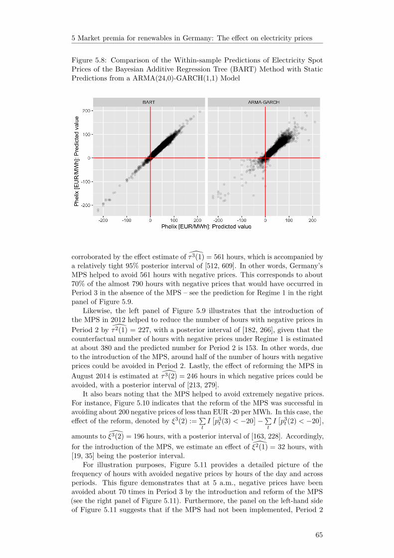
5 Market premia for renewables in Germany: The effect on electricity prices
Figure 5.8: Comparison of the Within-sample Predictions of Electricity SpotPrices of the Bayesian Additive Regression Tree (BART) Method with StaticPredictions from a ARMA(24,0)-GARCH(1,1) Model
corroborated by the effect estimate of τ3(1) = 561 hours, which is accompanied bya relatively tight 95% posterior interval of [512, 609]. In other words, Germany’sMPS helped to avoid 561 hours with negative prices. This corresponds to about70% of the almost 790 hours with negative prices that would have occurred inPeriod 3 in the absence of the MPS – see the prediction for Regime 1 in the rightpanel of Figure 5.9.
Likewise, the left panel of Figure 5.9 illustrates that the introduction ofthe MPS in 2012 helped to reduce the number of hours with negative prices inPeriod 2 by τ2(1) = 227, with a posterior interval of [182, 266], given that thecounterfactual number of hours with negative prices under Regime 1 is estimatedat about 380 and the predicted number for Period 2 is 153. In other words, dueto the introduction of the MPS, around half of the number of hours with negativeprices could be avoided in Period 2. Lastly, the effect of reforming the MPS inAugust 2014 is estimated at τ3(2) = 246 hours in which negative prices could beavoided, with a posterior interval of [213, 279].
It also bears noting that the MPS helped to avoid extremely negative prices.For instance, Figure 5.10 indicates that the reform of the MPS was successful inavoiding about 200 negative prices of less than EUR -20 per MWh. In this case, theeffect of the reform, denoted by ξ3(2) := ∑
tI[p3t (3) < −20
]−∑tI[p3t (2) < −20
],
amounts to ξ3(2) = 196 hours, with a posterior interval of [163, 228]. Accordingly,for the introduction of the MPS, we estimate an effect of ξ2(1) = 32 hours, with[19, 35] being the posterior interval.
For illustration purposes, Figure 5.11 provides a detailed picture of thefrequency of hours with avoided negative prices by hours of the day and acrossperiods. This figure demonstrates that at 5 a.m., negative prices have beenavoided about 70 times in Period 3 by the introduction and reform of the MPS(see the right panel of Figure 5.11). Furthermore, the panel on the left-hand sideof Figure 5.11 suggests that if the MPS had not been implemented, Period 2
65
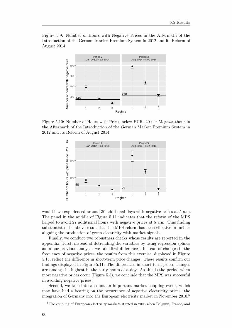
5.5 Results
Figure 5.9: Number of Hours with Negative Prices in the Aftermath of theIntroduction of the German Market Premium System in 2012 and its Reform ofAugust 2014
●
●
●
146
●
●
●220
Period 2Jan 2012 − Jul 2014
Period 3Aug 2014 − Dec 2016
1 2 3 1 2 3
200
400
600
800
Regime
Num
ber
of h
ours
with
neg
ativ
e pr
ice
Figure 5.10: Number of Hours with Prices below EUR -20 per Megawatthour inthe Aftermath of the Introduction of the German Market Premium System in2012 and its Reform of August 2014
●
●
●
50
●
●
●29
Period 2Jan 2012 − Jul 2014
Period 3Aug 2014 − Dec 2016
1 2 3 1 2 3
100
200
RegimeNum
ber
of h
ours
with
pric
e be
low
−20
EU
R
would have experienced around 30 additional days with negative prices at 5 a.m.The panel in the middle of Figure 5.11 indicates that the reform of the MPShelped to avoid 27 additional hours with negative prices at 5 a.m. This findingsubstantiates the above result that the MPS reform has been effective in furtheraligning the production of green electricity with market signals.
Finally, we conduct two robustness checks whose results are reported in theappendix. First, instead of detrending the variables by using regression splinesas in our previous analysis, we take first differences. Instead of changes in thefrequency of negative prices, the results from this exercise, displayed in Figure5.15, reflect the difference in short-term price changes. These results confirm ourfindings displayed in Figure 5.11: The differences in short-term prices changesare among the highest in the early hours of a day. As this is the period whenmost negative prices occur (Figure 5.5), we conclude that the MPS was successfulin avoiding negative prices.
Second, we take into account an important market coupling event, whichmay have had a bearing on the occurrence of negative electricity prices: theintegration of Germany into the European electricity market in November 2010.6
6The coupling of European electricity markets started in 2006 when Belgium, France, and
66

5 Market premia for renewables in Germany: The effect on electricity prices
Figure 5.11: Number of Hours with Avoided Negative Prices, by Hour and Period
●
●
●● ●
●
●
●
●
●
● ●● ●
● ●
● ● ● ● ●● ●
● ●
●
●
●
●
●●
● ●
●
●
●
●
●
●
●
●
●● ● ●
● ●
●
●
●
●
●
●
●
●
●
●
●
●
●●
●
●
●
●
●
● ●
●
●●
●
Period : 2; Jan 2012 − Jul 2014
Regime: 1
Period : 3; Aug 2014 − Dec 2016
Regime: 2
Period : 3; Aug 2014 − Dec 2016
Regime: 1
1 5 9 13 17 21 1 5 9 13 17 21 1 5 9 13 17 21
0
10
20
30
40
50
60
70
Hour
Num
ber
of h
ours
in w
hich
neg
ativ
e pr
ices
wer
e av
oide
d
To investigate this issue, we split Period 1 into two subperiods: Period 1a(January 2009 – October 2010) and Period 1b (November 2010 – December 2011),as Germany was connected to the joint European electricity market in November2010.
The results of this robustness check indicate that if the MPS had not beenin operation in Period 2 (January 2012 – July 2014), negative prices wouldhave occurred in about 450 hours, while the actual value amounts to 146 hours(lower left panel of Figure 5.16). Even though the point estimates of the numberof negative prices is somewhat higher compared to Figure 5.9, the absence ofdifferences between Period 1a and Period 1b indicates that this market couplingevent had no impact on the frequency of negative prices.
In addition, if the reform of the MPS had not taken place, we would haveobserved about even more hours with negative prices in Period 3 (see lower rightpanel of 5.16). As our estimate from Figure 5.9 of around 800 hours with negativeprices roughly lies in the middle of the two estimates for Regimes 1a and 1b,we conclude that Germany’s integration into the European electricity marketdid not have a bearing on the occurrence of negative prices. This conclusion issubstantiated by the evidence displayed in Figure 5.17, where we focus on highlynegative prices.
5.6 Conclusion
To reduce greenhouse gas emissions, an overwhelming number of countries promoterenewable energy technologies, most often, as in Germany, in the form of FITs.These tariffs are paid for each kWh of green electricity produced by renewable
the Netherlands connected their electricity markets. Germany and Luxembourg joined thiscommon market area in November 2010. In the meantime, more countries were connected to thecommon electricity market, such that the coupled market area covers more than 20 countries,standing for about 90% of Europe’s electricity consumption (Ringler, Keles, & Fichtner, 2017).The idea behind market coupling is to increase welfare by allowing electricity to flow from lowcost areas to high cost areas, resulting in price convergence (Keppler, Phan, & Le Pen, 2016).
67

5.6 Conclusion
energy technologies irrespective of whether the demand for electricity is low.In terms of RES capacity expansion, Germany’s FIT system, established in2000, proved highly successful and is thus widely seen as a role model for thepromotion of renewable energy technologies. Between 2000 and 2016, REScapacities increased ten-fold to reach 104 GW, thereby exceeding the capacityof conventional power plants in 2016 for the first time (BMWi, 2017). As aconsequence of the increasing RES capacities, prices on the wholesale electricitymarket decreased, which is commonly referred to as merit-order effect (Praktiknjo& Erdmann, 2016). In times of low demand, such as on Sundays or on publicholidays, the pressure on electricity prices due to a large supply of green electricitymay be so strong that prices turn out to be even negative.
To counteract these adverse effects, numerous countries have implementedpremium schemes with the aim of aligning green electricity generation withmarket signals. Under premium schemes, rather than getting fixed FITs (RES,2018), operators of renewable plants are commonly paid a bonus on top of thewholesale electricity price, thereby providing incentives to reduce production intimes of low electricity demand.
In this paper, using hourly day-ahead spot market prices from 2009 to 2016and the nonparametric method of Bayesian Additive Regression Trees, we haveanalyzed the efficacy of the German MPS in terms of reducing the frequencyof hours with negative prices. This method allows for the straightforward con-struction of counterfactual situations and predictions of hypothetical outcomes,such as the electricity prices in the absence of the MPS. Along with a very highpredictive power, this constitutes a distinctive feature of this method (Hill, 2011).
Based on such counterfactual analyses, we find that the implementation ofthe MPS in Germany in 2012 was quite effective in reducing the prevalence ofnegative electricity prices. Altogether, the introduction of the MPS and its reformin August 2014 helped to avoid some 560 hours with negative prices in the periodspanning January 2012 to December 2016, particularly in the morning hours.Without the MPS, negative prices would have occurred over about 790 hours,indicating that about 70% of potential hours with negative prices were avoided.Moreover, the MPS was successful in avoiding about 200 negative prices of lessthan EUR -20 per MWh. Given these results, we conclude that, compared toFIT systems with guaranteed payments, MPS are a more cost-effective measureto promote renewable energy technologies.
It bears noting, though, that a comprehensive cost-benefit analysis wouldalso take into account the implementation and transaction costs that arise dueto a MPS. Moreover, while it is beyond the scope of our analysis to provideany guidance on how to design optimal promotion systems, Andor and Voss(2016) suggest that if positive externalities arise from the installation of renewablecapacities, capacity-based instruments, such as tax cuts, should be employed,whereas generation-based instruments, such as FITs, would be preferable whenpositive externalities arise from the generation of green electricity. Yet, althoughcapacity-based subsidies are particularly suited to push new technologies, suchpromotion schemes have not been implemented in many countries so far. Whilethis also holds true for Germany, the country has recently improved the costefficiency of the promotion of renewable technologies by introducing a tenderingscheme in 2017, in which participants bid on a fixed remuneration per kilowatthourof green electricity, but are allowed to gain additional profits by direct marketing.
68

5 Market premia for renewables in Germany: The effect on electricity prices
5.A Appendix
Figure 5.12: Overlap in the Covariates across Time Periods
Solar [MW] Wind [MW]
Load [MW] Nuclear [MW] Phelix [EUR / MWh]
Allowance price [EUR / t CO2] Hard coal [MW] Lignite [MW]
0 10 20 0 10 20 30
30 40 50 60 70 80 0 5 10 15 −400 −200 0 200
5 10 15 0 5 10 15 20 0 5 10 15 200.00
0.05
0.10
0.15
0.20
0.00
0.01
0.02
0.03
0.04
0.00
0.02
0.04
0.06
0.0
0.2
0.4
0.6
0.00
0.05
0.10
0.15
0.0
0.1
0.2
0.3
0.00
0.01
0.02
0.03
0.00
0.25
0.50
0.75
Value
Den
sity
Period
Period 1: Jan 2009 − Dec 2011
Period 2: Jan 2012 − Jul 2014
Period 3: Aug 2014 − Dec 2016
Figure 5.13: Overlap in the Detrended Covariates across Time Periods
Solar [MW] Wind [MW]
Load [MW] Nuclear [MW] Phelix [EUR / MWh]
Allowance price [EUR / t CO2] Hard coal [MW] Lignite [MW]
−5 0 5 10 15 20 25 −10 0 10 20
−20 −10 0 10 20 −15 −10 −5 0 5 −400 −200 0
−4 −2 0 2 −10 −5 0 5 10 −15 −10 −5 0 50.00
0.05
0.10
0.15
0.20
0.00
0.01
0.02
0.03
0.04
0.00
0.02
0.04
0.06
0.08
0.0
0.1
0.2
0.3
0.4
0.00
0.05
0.10
0.15
0.0
0.2
0.4
0.6
0.00
0.01
0.02
0.03
0.0
0.1
0.2
0.3
0.4
Value
Den
sity
Period
Period 1: Jan 2009 − Dec 2011
Period 2: Jan 2012 − Jul 2014
Period 3: Aug 2014 − Dec 2016
69

5.A Appendix
Figure 5.14: Comparison of the Within-sample Predictions of Electricity SpotPrices of the Bayesian Additive Regression Tree (BART) Method with StaticPredictions from a AR(24)-GARCH(1,1) Model
Figure 5.15: Difference in Price Changes, by Hour and Period using DifferencedVariables
●●
● ●
●
●
● ● ●
● ● ●●
●● ● ● ●
● ●
●
●
●●
● ● ●●
● ●
●●
●
● ● ●● ● ● ●
●
● ●
●
● ●●
● ●●
●●
●
●●
●
●
● ●●
●
●● ●
●
● ●
● ●●
●
●
Period : 2; Jan 2012 − Jul 2014
Regime: 1
Period : 3; Aug 2014 − Dec 2016
Regime: 2
Period : 3; Aug 2014 − Dec 2016
Regime: 1
1 5 9 13 17 21 1 5 9 13 17 21 1 5 9 13 17 21
0
10
Hour
Cha
nge
in p
rice
[EU
R/M
Wh]
70
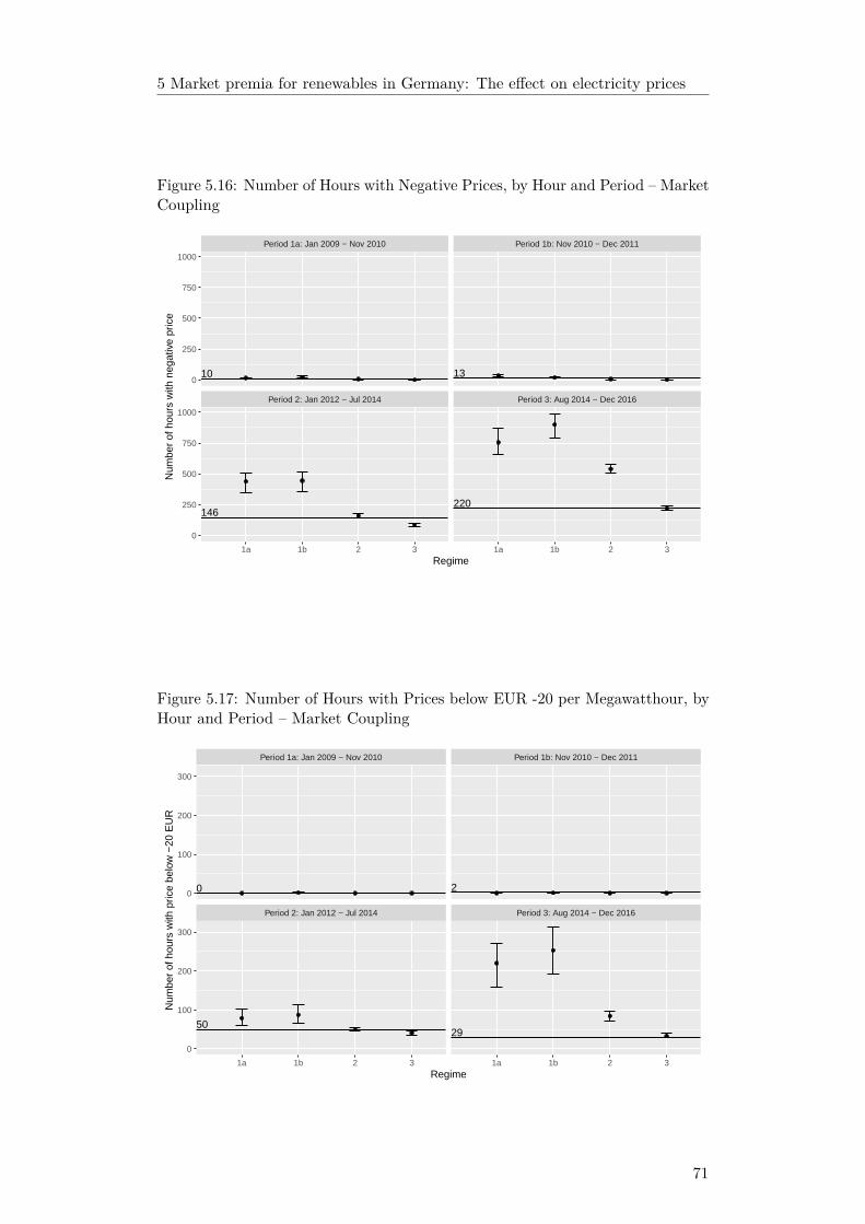
5 Market premia for renewables in Germany: The effect on electricity prices
Figure 5.16: Number of Hours with Negative Prices, by Hour and Period – MarketCoupling
10
146
13
220
Period 2: Jan 2012 − Jul 2014 Period 3: Aug 2014 − Dec 2016
Period 1a: Jan 2009 − Nov 2010 Period 1b: Nov 2010 − Dec 2011
1a 1b 2 3 1a 1b 2 3
0
250
500
750
1000
0
250
500
750
1000
Regime
Num
ber
of h
ours
with
neg
ativ
e pr
ice
Figure 5.17: Number of Hours with Prices below EUR -20 per Megawatthour, byHour and Period – Market Coupling
0
50
2
29
Period 2: Jan 2012 − Jul 2014 Period 3: Aug 2014 − Dec 2016
Period 1a: Jan 2009 − Nov 2010 Period 1b: Nov 2010 − Dec 2011
1a 1b 2 3 1a 1b 2 3
0
100
200
300
0
100
200
300
Regime
Num
ber
of h
ours
with
pric
e be
low
−20
EU
R
71

5.A Appendix
72

Chapter 6
Equal access to primary care:A benchmark for spatialallocation1
Abstract
Using a greedy algorithm together with very fine spatial data, we calculate anoptimal allocation of general practitioners in Germany. This benchmark allowsus to not only identify regions experiencing over- and undersupply but also topropose how general practitioners should locate to relax existing uneven regionaldistribution. Our results suggest that overall there were 6% too few GPs inGermany to provide equal primary care for every person in 2019 and that moreGPs should be placed in rural regions. However, we do not observe that residentsof rural regions experience stronger undersupply than residents of urban regions.
Keywords: Optimization, Regional data, Health, Medical access, Redistribution
1This paper is jointly written with Alexander Haering and Anna Werbeck.
73

6.1 Introduction
6.1 Introduction
Equal access to health care is fundamental for a reliable health care system. Yet,uneven geographic distribution of physicians causes concern across the memberstates of the Organisation for Economic Co-operation and Development (OECD)and, although it has been in the centre of health care discussion for many decades,it still remains the single most commonly named issue in the health sector (OECD,2014). Various policies have been installed to tackle this problem. They aim (i) atmedical students to recruit new physicians to serve in undersupplied areas, (ii) atcurrent physicians to redistribute the physician workforce by financial incentivesor regulations, or (iii) at an integration of innovative forms of care (OECD, 2014).To clearly evaluate these policies, we need a tool proposing efficient allocationsof physicians.
In this paper, we calculate a benchmark of smallest quantity and optimalallocation of general practitioners (GPs) for Germany in 2019. We first calculatethe demand for GP visits on a small regional scale based on age and gender. Wethen optimize the number of GPs by allocation under the two constraints thateach resident has access to at least one GP within reasonable driving time andthat each GP has limited capacity of patient contacts. Because there usually toofew GPs overall, or the GPs are not optimally distributed, these constraints areusually not satisfied in practice.
Germany is particularly suited as a first testing ground. Equal access tohealth care is manifested in the very first paragraph in Book I of the Social Code(SGB I, Sozialgesetzbuch I ). It determines that all social rights, including healthcare, apply uniformly to all residents. In the German health care system, generalpractitioners2 constitute the centre of the ambulatory care sector (§73 SGB V)and are generally the first medical point of reference for patients. Therefore,equal access to health care requires, besides quality, a sufficient number of generalpractitioners combined with an adequate distribution among different regions.However, the problem cannot be solved by massively increasing the number ofGPs, as Book V of the Social Code also demands cost-effectiveness of healthcare services (§12 SGB V). Incorporating these legislative demands, we useguidelines and data on the current workload of GPs to determine the area anddemand a single physician can cover. Using these constraints, we formulate ourGerman-specific optimization problem as follows: What is the optimal numberand regional allocation of general practitioners such that each resident can reacha GP within 15 minutes driving time (Federal Institute for Research on Building,Urban Affairs and Spatial Development, 2005) and that GPs serve within theirlimited capacity of 13, 000 annual cases?3
The political discussion in Germany is centered on two major issues. First,an overall shortage of general practitioners and second, an especially severeundersupply in rural regions. Our benchmark allocation suggests that there wereindeed 6% too few GPs in Germany in 2019. Also, we find uneven geographicdistribution of GPs that is more pronounced in less densely populated areas.However, the maldistribution does not translate into an especially severe under-
2In this study, we follow the specification of general pracitioners as specified in §73 SGB V,excludinig paediatricians. We include general physicians, internists without a specializationwho have chosen to participate in GP care, doctors who are listed in the register of doctors inaccordance with §95a IV/V 1 and those who were participating in GP care up to December31st, 2000.
3We obtained this number from (National Associations of Statutory Health InsurancePhysicians’ & Verband der niedergelassenen Arzte Deutschlands, 2018).
74

6 Equal access to primary care: A benchmark for spatial allocation
supply of rural dwellers’ health care demand. Put differently, even though ourbenchmark solution would place more GPs in rural regions, we do not see thatresidents of less densely populated areas experience structurally more undersupplythan those in more densely populated ones. However, there is a general level ofundersupply which might be relaxed with a more efficient GP-allocation.
We bridge the gap between two main strands of literature: operations researchand regional variation in health care. We do so by generating a benchmarkallocation for GPs in Germany using the methodology developed in the operationsresearch literature to inform our view on regional differences in health care access.
Researchers in the field of operations research in health care developedan algorithmic toolkit for location-allocation problems (Daskin & Dean, 2005)and applied it to several health care facilities (see Rais & Viana, 2011, for awell-structured overview). Related to our research, some studies calculate theoptimal allocation of health care facilities to maximize accessibility under differentconstraints. Marianov and Taborga (2001), for example, set up an allocationplan for health-care centers maximizing coverage for a low-income populationwithin pre-specified distance. Harper, Shahani, Gallagher, and Bowie (2005)develop a simulation model accounting for patients traveling to the providers,resource capacities, heterogeneous patient needs and different transport modes.We contribute to this research field by presenting a benchmark for the optimalallocation of GP practices in Germany, accounting for local geography, resourcecapacities of GPs, and heterogenous patient needs. In addition, we account forcorrelations between regional indicators and health care supply and demand.
In health economics, several studies investigate regional disparities in healthcare and their sources (see, e.g., Finkelstein, Gentzkow, and Williams, 2016;Johansson, Jakobsson, and Svensson, 2018; Salm and Wubker, 2020). Otherstudies develop solutions to this global problem. Sutton and Lock (2000), forexample, derive a resource allocation formula incorporating regional variation inhealth care using data from 15 regions in Scotland. Others evaluate policies thathave been implemented to tackle the challenge of undersupply of general healthcare (see, e.g., Zhang, Baik, Fendrick, & Baicker, 2012). Yet, what is missing isa reference for an optimal number of GPs and their practice locations ensuringeveryone’s health care demand is satisfied on a small-scale. Without a benchmarkit remains unclear whether or not the resultant quantity and practice locationsof GPs meet the respective needs sufficiently and efficiently. Our contribution isto fill this gap and propose such a benchmark for Germany.
The rest of the paper is structured as follows: the next section describes ourdata, followed by the methodology. In the fourth section, we present our findings,section five shows sensitivity analyses, and section six concludes.
6.2 Data
Driving times
Our computed driving times are based on grid cells from the RWI-GEO-GRID(Breidenbach & Eilers, 2018). The RWI-GEO-GRID database contains socioeco-nomic data for Germany on 218,875 populated 1km2 grid cells.4 We determinedriving time by car from each populated grid cell to all populated grid cellswithin 40 km radius using the Open Source Routing Machine program (Luxen& Vetter, 2011), based on OpenStreetMap (Haklay & Weber, 2008) road data,
4The grid cells are aligned to the EU-wide INSPIRE Directive (Bartha & Kocsis, 2011).
75

6.2 Data
which contains nearly the complete German road network (Barrington-Leigh &Millard-Ball, 2017). A radius of 40 km ensures that we include all grid cells thatcan be reached within 15 minutes.
This procedure leaves us with around 600, 000, 000 driving times. Next, wediscard driving times exceeding 15 minutes to avoid unnecessary calculationsand because Federal Institute for Research on Building, Urban Affairs andSpatial Development (2005) demands that every person reaches one GP within amaximum of 15 minutes. This results in around 170, 000, 000 driving times.
Current GP Allocation: the Status Quo
The Regional Associations of Statutory Health Insurance Physicians’ (RASHIP)contains information on all contract physicians and contract psychotherapists intheir respective region. NASHIP is their national umbrella organization. RA-SHIP and NASHIP provide aggregated numbers of GPs on federal state levels.However, for our study we need the exact practice location. Therefore, we utilizedata from the official on-line search engines of both organizations.5 The searchengines are accessible to the German population to search for doctors in allfields. Yet, physicians have to agree to be listed in the NASHIP and/or RASHIPonline database. This potential self-selection into the search-engines may lead totwo problems: Either, when focusing only on one database, we are left with anundercount as physicians that do not agree to be listed in the chosen search-engineare not part of our set; or, when using the two databases, we are left with anovercount when a physician is listed in both. To avoid these problems, we usedboth data sources. In addition, we also created a third data-source, consisting ofthe intersection of both data sets. To verify our approach, we aggregated ourGP-count on federal state level and compared it to the official number providedby NASHIP (2018). For every federal state, we chose the data source with theGP-count closest to the official number. Table 6.1 summarizes the number ofGPs obtained from the three sources. In total, there are 55,006 GPs in the dataset, representing the status-quo allocation.
Table 6.1: Number of GPs by Source
Data source N
NASHIP 33,031RASHIP 15,140Intersection 6,835
Total 55,006
Note: State of data as of 2019
GP visits
Furthermore, we use data from the SOEP (Goebel, Grabka, Liebig, Kroh, Richter,Schroder, & Schupp, 2019), which is the largest representative longitudinal panelof private households in Germany. We utilize wave 2016 because, besides ageand gender, it contains self-reported number of annual visits to the doctor. This
5See appendix 6.A for all 18 webpages.
76

6 Equal access to primary care: A benchmark for spatial allocation
allows us to calculate the expected number of cases in each grid cell. Our resultingdata set contains 24, 418 observations. Table 6.2 shows the mean and standarddeviation for our variables of interest.
Table 6.2: Summary Statistics Regression Tree
Mean SD
Age 48.663 17.617Female 0.542 0.498# visits doctor 9.092 14.624Source: SOEP wave 2016 (Goebel, Grabka,Liebig, Kroh, Richter, Schroder, & Schupp,2019)
Characteristics of municipalities
To examine whether a shortage of GPs only appears in less densely populatedregions and which regional patterns are correlated with over- or undersupply, weuse additional municipality characteristics.6
For ease of interpretation, we generate dummy variables for rural and suburbanareas following the classification of Dijkstra and Poelman (2014) to assort allGerman municipalities with respect to their population density. Sensitivityanalyses (see section 6.5) show that this aggregation of grids does not influenceour results. We calculate a commuter index by
(in commuter− out commuter)population (6.1)
using data from the German Federal Agency of Employment (BA, 2008). Wealso calculate a migration index in the same way:
(in migration− out migration)population . (6.2)
Furthermore, we add employment-rate, self-employment rate and the businesstax from (Federal Office for Building and Regional Planning, 2020) as measuresof economic power.7
In addition, we use house and rent prices, as derived from the FDZ data set(see Boelmann & Schaffner, 2018, for a description). Table 6.3 summarizes themean and standard deviation of our variables.
6Because the area of municipalities may vary in Germany over time, e.g. due to mergers,and our data sets are not from the exact date in 2019, there is some mismatch and we do nothave information on all 10, 848 municipalities.
7Employment rate and business tax are only available on the level of municipality association,self-employment rate is on district level. Since municipalities are sharply defined in both levelsof aggregation, it enables us to merge the respective value of employment rate and business taxon municipality level.
77

6.3 Methodology
Table 6.3: Municipality Characteristics
Mean SD
Rural 0.757 0.429Suburban 0.240 0.427Urban 0.004 0.060Business tax (in e per resident) 414.637 744.131Commuter index 0.086 0.152Employment rate (in employees per 100 potential workers) 61.141 5.546Migration index 0.00 0.01House price (in e per km2) 1781.441 855.253Rent price (in e per km2) 6.811 1.548Self-employment rate (in self-employed per 100 workers) 115.053 17.362Note: Rural, suburban and urban are dummy variables.
6.3 Methodology
Set cover problem
Our unique combination of data sets helps us to determine the optimal numberand regional allocation of GPs in Germany under the following constraints: Allresidents can reach at least one GP within 15 minutes driving time and GPsserve within their limited capacity of 13, 000 annual cases. That is, we face acapacitated set cover problem. The set cover problem is a central problem incombinatorics with wide ranging applications, see, as examples, Vazirani (2001)or Korte and Vygen (2018).
Initially, we ignore the limited capacity. We set up a general uncapacitated setcover problem, where one determines the smallest sub-collection from a collectionof sets S = {S1, S2, . . . , Sl} that covers a universe of elements U , i.e., everyelement in U appears in at least one of the subsets of S. Here, the universe isU = {g1, . . . , gn}, where gi is the ith 1km2 grid. We define Si as
Si := {gj | d(gj , gi) ≤ 15min},
where d(gi, gj) ≥ 0 is the asymmetric driving time from gi to gj . This impliesthat Si consists of all grid cells from where grid gi is reachable within 15 minutes.As d(gi, gi) = 0, Si always includes gi.
Figure 6.1 shows four exemplary sets from our data. In all four figures, thedark blue grid cell at the center depicts gi, the potential location of a generalpractitioner. The differently colored cells in the surrounding show all grid cellsfor which gi is reachable within 15 minutes. We see that the shapes of the setsvary. This is driven by street infrastructure, classified by 15 speed types andgeographical conditions.
In the capacitated case, we restrict the demand to be covered by a singleset to be below 13,000 patient-physician contacts, i.e., cases, per year, so thateach set Si consists of the grids containing the cases serviced by the ith GP. Thismight require placing multiple GPs in one grid to satisfy the demand.8
8Because we operate within a resolution of 1km2, we do not differentiate between GPsworking in a joint practice and those who do not.
78

6 Equal access to primary care: A benchmark for spatial allocation
Figure 6.1: Grids from where the Center Grid can be reached within 15 Minutes.
0
5
10
15
Driving timein minutes
Greedy approximation
Because the set of possible solutions grows exponentially with the number of setsin S, the problem becomes too complex to be solved exactly. Therefore, we usethe capacitated variant of the greedy approximation algorithm (Chvatal, 1979;Lovasz, 1975). Feige (1998) shows that the basic greedy approximation givesreasonably good approximations to the true solution while scaling well to largedata sets. Vazirani (2001, chap. 29) shows why the approximation is very hardto improve.
The basic idea of our greedy approximation is to iteratively distribute doctorsacross the grid. Given that in Germany most GPs serve in private practiceswith not more than a few general practitioners working together, we introducea penalty to avoid placing more than 10 GPs per grid. We start from a greenfield without any doctors. In every iteration, we choose the set with the mostuncovered demand, until every case is covered. Here, covering demand meansassociating cases with a GP. Parka and Honga (2009) add a pre-processing stepto the greedy approximation for the capacitated case, where one iteratively coversdemand (here, 13, 000 cases), until no sets exceeding the capacity remain. Figure6.2 gives a short illustration of the two algorithms.
For our implementation of the uncapacitated greedy algorithm in R we buildon the RcppGreedySetCover package (Kaeding, 2018). For all pre-processing stepsin case of the capacitated set cover algorithm, we create a fast C++ implementation.
79

6.3 Methodology
Figure 6.2: Set Cover Algorithm Uncapacitated
Uncapacitated
Find set with mostuncovered grids
Increment GP count by one for this set
Cover all remaining cases for this set
Are all grids covered?
Yes
Stop
No
Pre-processing
Find set with mostuncovered demand
Increment GP count by one for this set
Cover 13, 000 cases for this set
Is the uncovered demandless than 13, 000 in every set?
Yes
Rununcapacitated
No
Feeding the greedy algorithm: calculating the number of cases
To calculate the adequate distribution of general practitioners, we account forthe expected number of cases in each grid cell. The SOEP 2016 data on numberof visits to the doctor’s office provides us with a proxy for medical demand. Weassume patient subgroups with an approximately constant number of visits. Assuch, we use a regression tree to forecast demand, which is suitable for identifyingsubgroups. We calculate a regression tree with age and gender as explanatoryvariables to forecast demand (see Table 6.2). While additional variables mightimprove prediction, we can only use those variables which are available in boththe SOEP 2016 data and the RWI-GEO-GRID. However, we assume that ageand gender are the most relevant variables and capture health demand fairly well.
For our estimation, we use the R package rpart (Therneau & Atkinson, 2019).Figure 6.3 shows our final tree9. The interpretation is straightforward. For exam-ple, a female subject (Female = 0, right branch) Age < 28 is expected to visitthe doctor’s office 8 times a year.10 We then use our regression tree to computethe expected number of GP visits for each 1km2 grid cell using the demographicdata provided by the RWI-GEO-GRID database. As an example, the city ofEssen has a population of some 0.6 million persons with an approximate demandof 5 million cases per year.
9Because we only have two exogenous variables, we use a simple model.10Interestingly: at Age > 75 the number of expected visits to the doctor is independent of
the gender with 13 visits a year.
80

6 Equal access to primary care: A benchmark for spatial allocation
Figure 6.3: Regression Tree Number of Visits to the Doctor per Year
Note: Calculation based on SOEP wave 2016, endogenous variable isself-reported number of visits to the doctor per year, R2 = 0.023.
Regressions
To examine whether our variables of interest, excess GPs and uncovered demand,are correlated with municipality characteristics, e.g. population density, werun additional regressions. We aggregate our grid data on municipality level,assigning each grid to the municipality with which it has the largest intersectingarea.11 In addition, we look at a commuter index as well as a migration indexfor municipalities. First, we define our dependent variable as
di := Nobservedi −Ngreedy
i , (6.3)
i.e. the difference between Nobservedi , the observed number of GPs in the ith
municipality, and Ngreedyi , the number of GPs needed to achieve full support
in the ith municipality. Therefore, we can interpret di as residual, measuringexcess number of GPs in a municipality. On these terms, an optimal allocationof GPs would result in di equal to zero for all i and our coefficients should notpick up correlation with the excess number of GPs. Figure 6.4 shows a map ofthe dependent variable.
We use di from (6.3) and specify our regression as:
di = α0 + α1rurali + α2suburbani + α3commuteri+α4migrationi + β>econpoweri + fspatial(si) + γ>xi + εi.
(6.4)
In equation (6.4), rurali and suburbani are dummy variables indicating ruralor suburban municipalities, where urban is the reference category. α0, . . . , α4 areregression coefficients, β and γ are vectors of regression coefficients. The variablecommuteri represents our commuter index, migrationi the migration index.econpoweri incorporates the variables unemployment rate, self-employmentrate and business tax that we report separately. Depending on our modelspecification, we add additional controls: fspatial(si) is a spatial effect accountingfor regional dependencies and vector xi contains rent and housing prices of
11In Section 6.5 we provide evidence that our results are not influenced by this aggregation.
81

6.3 Methodology
Figure 6.4: Excess GPs in Germany by municipality
Note: Because outliers would otherwise dominate the color scale,values outside the interval [−100, 100] are shown via annotation.
municipality i. We additionally add dummies for the federal states.12 Thesmooth spatial effect fspatial accounts for spatial dependence across neighboringmunicipalities unexplained by the covariates. We model fspatial via thin-plateregression splines (cf. Wood, 2003, for further details).
We estimate the model using the R package mgcv (Wood, 2011). Thefixed effects on federal state level account for heterogeneity in the institutionalframework of Germany, for instance varying incentives for GPs to practice insmaller towns. All metric independent variables are scaled by one standarddeviation to achieve effect comparability.
We shall also investigate the German population generating health caredemand by running additional regressions to study regional patterns correlatedwith uncovered cases. We again focus on the three classifications of municipalitieswith regards to population density as our main variable and a commuter as wellas a migration index. To this end, we create an index measuring the percentage ofdemand which, given our constraints, cannot be covered, i.e., maximal drivetime of15 minutes and a GP-capacity of 13,000 cases per year. Notably, these uncoveredcases only exist in case of the status quo, in the benchmark situation all healthcare demand is covered perfectly. We assume that each person frequents theclosest GP. Then we classify each case as uncovered if it exceeds the capacity ofthe providing GP. We define our index as the percentage of uncovered cases in
12We add two dummies for North Rhine-Westphalia, because it is divided into two RASHIPs.In addition, we use a single dummy for all city-states, which only have one municipality each.Therefore, we add 15 federal state dummies to our regression analysis.
82

6 Equal access to primary care: A benchmark for spatial allocation
Figure 6.5: Uncovered cases in Germany by municipality
each municipality. This is an approximation because of the following two reasons:(i) In reality, GPs probably still provide care when above capacity. (ii) Personsmight switch to a GP further away who is not overcapacitated. However, theselimitations mainly concern the overall level of undersupply, while our index allowsus to compare the level of potential undersupply across regions.
More precisely, we assume the number of cases a GP covers in a grid g isproportional to the overall demand, i.e.,
ck = λck∑j I[grids j and k share same GP]cj
, (6.5)
where ck denotes number of cases covered, i.e., treated patients, in grid k, λ is thecapacity all GPs providing care for this grid have. ck is the number of cases, i.e.,sick patients, in grid k. We define the dependent variable for every municipalityi as the percentage of uncovered cases by
ui := 100∑j∈i I[cj > cj ](cj − cj)∑
j∈i cj. (6.6)
This gives us the percentage of uncovered cases, i.e., unsatisfied health caredemand generated by each municipality. As an illustration, assume that munic-ipality i has a demand of 20, 000 cases, and a single GP that is closest to allpatients in i. Assume further that the GP does not cover any cases of patientsfrom other municipalities. Then, this municipality i is left with 7, 000 uncoveredcases. This equals a share of 100 × 7,000
20,000 = 35%. Figure 6.5 shows a map ofvariable u. Note that our approach assumes that each patient chooses her nearestGP within 15 minutes driving time. Therefore, it is not necessary that the GP
83

6.4 Results
practice is located in the patient’s municipality. For our second regression, weuse the same controls as in (6.4) and u as the dependent variable.
6.4 Results
This section discusses our results. The current political discussion is centeredon two major concerns: First, an overall shortage of general practitioners, andsecond, an especially severe undersupply in rural regions. We now investigatethese claims through the lens of our analysis.
Figure 6.6 shows the status-quo allocation compared to our benchmark alloca-tion on a grid level. The left panel shows the distribution of general practitionersin Germany as of 2019. The overall number of active general practitioners was55, 006. As expected, densely populated areas like the city-states of Berlin andHamburg as well as other large regions like Munich or the Ruhr area have ahigh density of GPs. The right hand panel of Figure 6.6 shows our bench-mark distribution of GPs in Germany. We determine the optimal number ofGPs needed in 2019 to be 58, 144. This is fairly similar to that of the actualdistribution. Remarkably, the optimal number of GPs is fairly close to theactual number of active GPs in 2019. We see a shortage of 3, 138 GPs (≈ 6%).Still, we take this difference as noteworthy. In our benchmark, GPs are moreevenly spread out across Germany, resulting in complete coverage. The distribu-tions differ mainly in densely populated areas such as Munich or the Ruhr area.Here, our benchmark solution places fewer GPs than there are in the status quo.Furthermore, more GPs are located in the city-centers, which are easy to reach 13.
Figure 6.6: Distribution of General Practitioners in Germany
Comparison of GPs allocation under status-quo and ourbenchmark allocation - grid level.
13It should be noted that our model does not account for the costs of the location, so that itmight be more cost-efficient to place GPs elsewhere even though this would mean that moreGPs are needed.
84

6 Equal access to primary care: A benchmark for spatial allocation
We now turn to the claim that Germany faces an especially severe undersupplyin rural regions. We start off by examining whether a shortage of GPs onlyappears in a small number of cities or regions, or if it is a broader issue. For thisanalysis, we consider the excess number of GPs in a municipality i calculatedby Nobserved
i −Ngreedyi (see equation (6.3)). Thereby, we take the allocation of
GP practices suggested by the greedy algorithm as the benchmark. Compared tothis optimal solution, we assess whether or not there are too many or too fewGP practices in one region.
Table 6.4 summarizes the excess number of GPs in German municipalities.It reports the total number as well as numbers split into three categories assuggested by EUROSTAT (see Dijkstra & Poelman, 2014, for further details):cities (densely populated), towns and suburbs (intermediate density) and ruralareas (thinly populated). This gives us the opportunity to gain more insightsregarding the claim of undersupply being primarily a problem of rural regions.
The overall picture reveals that of the 11, 004 municipalities 3, 688 face anexcess of GPs compared to the benchmark allocation, 3, 084 experience a shortageof GPs, and 4, 232 are served optimally.
When split into the three regional categories, the data show that of the 125densely populated areas, 77 face an excess of general practitioners, while 45 facea shortage of GPs. Of the intermediately populated regions 1, 485 have an excessof GPs, 864 a shortage. And in the low populated regions 2, 126 face an excess,2, 175 a shortage of GPs and in 3, 953 rural regions the benchmark solutionwould not change the number of GPs from the current situation. Consideringrelative numbers, 36% of cities, 33% of towns and suburbs and only 25% of ruralareas face an undersupply of GPs. This does not show a clear-cut picture of thesituation. We therefore regress our calculated excess number of GPs on the threeregion categories.
Table 6.4: Municipality with excess/shortage of GPs by Population Density
Population Density Number of municipalitiesExcess GPs Shortage GPs Optimal GPs Total
Cities 77 45 3 125(66%) (36%) (2%) (100%)
Towns/Suburbs 1,485 864 276 2,625(57%) (33%) (10%) (100%)
Rural 2,126 2,175 3,953 8,254(26%) (26%) (48%) (100%)
Total 3,688 3,084 4,232 11,004(34%) (28%) (68%) (100%)
Notes: Share in parenthesis, classification based on Dijkstra and Poelman (2014)
Table 6.5 summarizes our regression results for excess number of GPs (seeequation (6.4)). In specification (1), we run a simple OLS regression with dummiesfor regional categories as explanatory variables. In (2), we additionally include thecommuter and migration index. In (3) we add the three measures for economicpower. Then, starting in (4), we include our smooth spatial effect to account forpartial dependence across neighboring municipalities. In specification (5), weadd federal state fixed effects. Lastly, in (6) we include rent and house prices as
85

6.4 Results
controls for costs of living.In all specifications, we observe a stable negative effect of suburban areas
compared to cities as our baseline. This effect is even more pronounced whenlooking at rural areas (p < 0.001, two-sided χ2 test). This suggests that there isindeed a disparity of rural and suburban areas after controlling for other factorsin terms of GP practices. Furthermore, the results show a negative correlationbetween excess number of GPs and a region’s commuter index (p < 0.001),implying that regions with higher in-commuting have fewer excess GPs. Thepicture is reversed for the migration index. We find a positive correlation,indicating that regions with higher in-migration have more excess GPs. Interms of our measures of economic power the results are mixed. Business taxes(p < 0.001) and employment rate (p < 0.050) are negatively correlated with excessnumber of GPs, whereas self-employment rate (p > 0.050) does not correlate withexcess number of GPs. The results suggests that there might be other factorsdriving the uneven geographic distribution of GPs.
Let us take a step back. If we focus solely on the location of GP practices,we miss the actual question of concern: does a structural lack of rural GPs leadto structural failure to satisfy health care demand of rural dwellers’ health caredemand? A crucial point why this question may not be addressed by lookingonly at the location of GP practices: doctors do not necessarily provide careexclusively to the residents of the municipality in which their practice is located.
To answer this question, we start by looking at what proportion of health caredemand of residents in one specific municipality remains unsatisfied. Flippingthis indicator around, this translates into the question: how much more would theGPs accountable for dwellers of one municipality have to work such that all healthcare demand is satisfied? This results in the proportion of unsatisfied health caredemand being equal to zero, just like in case of our benchmark scenario.
We run a regression for the linkage between unsatisfied health care demandand population density as well as the commuter and migration indices andour economic power measures. Table 6.6 reports the regression results for thepercentage of uncovered cases, i.e., unsatisfied health care demand (see equa-tion (6.6)), with the same specifications as in our model for excess number of GPs.
86

6 Equal access to primary care: A benchmark for spatial allocation
Table 6.5: Regression: Excess Number of GPs and Municipality Characteristics
(1) (2) (3) (4) (5) (6)
Intercept 21.62∗∗∗ 21.24∗∗∗ 20.87∗∗∗ 23.29∗∗∗ 8.80∗∗∗ 10.62∗∗∗(1.27) (1.28) (1.63) (1.81) (1.61) (1.67)
Rural −22.31∗∗∗ −21.70∗∗∗ −21.96∗∗∗ −22.24∗∗∗ −7.27∗∗∗ −7.74∗∗∗(1.28) (1.28) (1.29) (1.29) (1.14) (1.15)
Suburban −21.31∗∗∗ −20.83∗∗∗ −20.98∗∗∗ −21.04∗∗∗ −5.92∗∗∗ −6.17∗∗∗(1.28) (1.29) (1.29) (1.29) (1.14) (1.14)
Commuter index −0.36∗∗∗ −0.39∗∗∗ −0.37∗∗∗ −0.36∗∗∗ −0.36∗∗∗(0.08) (0.08) (0.08) (0.07) (0.07)
Migration index 0.12 0.10 0.13 0.11 0.16∗(0.08) (0.08) (0.08) (0.07) (0.07)
Business tax −0.27∗∗∗ −0.24∗∗ −0.26∗∗∗ −0.24∗∗∗(0.08) (0.08) (0.07) (0.07)
Employment rate −0.06 −0.18 −0.20∗ −0.20∗(0.08) (0.10) (0.09) (0.08)
Self-employment rate 0.22∗∗ 0.08 0.02 0.02(0.08) (0.10) (0.09) (0.09)
Spatial effect ! ! !
State FE ! !
Housing prices !
AIC 74,659.72 74,640.22 74,623.80 74602.10 71,414.99 71,404.30N 10,688 10,688 10,688 10688 10,688 10,688Adjusted R2 0.03 0.03 0.03 0.04 0.29 0.29Note: All independent variables are scaled by standard deviation, the baseline is category urban, thethree German city-states are represented by one fixed effect, standard errors reported in parentheses,∗∗∗p < 0.001; ∗∗p < 0.01; ∗p < 0.05, the mean of excess GPs is −0.37 with a standard deviation of 8.01.
Notably, we do not observe a correlation between unsatisfied health caredemand and rural regions. It contrasts the clear association between less denselypopulated areas and lower levels of excess GPs (see Table 6.5). This might bedue to two factors: (1) GPs might be distributed near the outskirts so that theycan cover demand outside the city as well; (2) by design, our index for uncoveredcases is not symmetric in oversupply: It might be the case that parts of a cityare strongly oversupplied, while other parts are strongly undersupplied (i.e.,local oversupply does not reduce overall undersupply). If we look at the resultsregarding the commuter index, we find a positive correlation with uncoveredcases (p < 0.001). This is a reversed picture compared to our results for thecorrelation with excess number of GPs: Regions with higher in-commuting havemore excess GPs. Yet, the correlations between uncovered cases and migrationindex or economic power measures are not significant.
In summary, we find mixed results regarding the two main issues of an overallshortage of GPs in Germany and an especially severe undersupply of rural regions.We find only a small discrepancy in the overall number of GPs, which we regardas noteworthy but not necessarily as a major cause for concern. With regard tothe inequity in regional health care markets, our results are inconclusive. Whenwe look at the supply side, i.e., the allocation of GPs, our benchmark solutionwould increase the number of rural doctors. However, we do not find evidencefor structural failure to satisfy rural health care demand. Our additional analysissuggests that there are likely other factors capturing a region’s unmet health caredemand.
87

6.5 Sensitivity analysis
Table 6.6: Regression: Percentage of Uncovered Cases and Municipality Charac-teristics
(1) (2) (3) (4) (5) (6)
Intercept 29.68∗∗∗ 30.43∗∗∗ 44.20∗∗∗ 30.03∗∗∗ 28.56∗∗∗ 30.75∗∗∗
(3.57) (3.57) (4.56) (5.13) (5.57) (5.86)Rural −0.30 −1.48 −0.07 −0.35 −1.03 −1.57
(3.58) (3.59) (3.60) (3.59) (3.69) (3.72)Suburban −1.98 −2.89 −1.58 −1.98 −2.38 −2.69
(3.59) (3.60) (3.61) (3.59) (3.68) (3.69)Commuter index 0.67∗∗ 0.76∗∗∗ 0.79∗∗∗ 0.90∗∗∗ 0.89∗∗∗
(0.22) (0.22) (0.22) (0.23) (0.23)Migration index −0.30 −0.34 −0.34 −0.30 −0.25
(0.22) (0.23) (0.23) (0.24) (0.24)Business tax −0.11 −0.02 0.02 0.03
(0.22) (0.22) (0.22) (0.22)Employment rate −0.95∗∗∗ −0.29 −0.35 −0.34
(0.22) (0.30) (0.31) (0.31)Self-employment rate −0.70∗∗ 0.37 −0.08 −0.08
(0.08) (0.10) (0.09) (0.09)
Spatial effect ! ! !
State FE ! !
Housing prices !
AIC 96,683.20 96,676.09 96,658.11 96,483.05 96,456.40 96,458.37N 10,688 10,688 10,688 10,688 10,688 10,688Adjusted R2 0.00 0.00 0.00 0.02 0.03 0.03Note: All independent variables are scaled by standard deviation, the baseline is the urban category, thethree German city-states are represented by one fixed effect, standard errors reported in parentheses,∗∗∗p < 0.001; ∗∗p < 0.01; ∗p < 0.05, the mean of uncovered cases is 28.28 with a standard deviation of21.97.
6.5 Sensitivity analysis
Influence of aggregation on regression results
Our regression results may depend on the aggregation of grids to the municipalitylevel. To test this, we carry out an experiment where we create random partitions,by iteratively merging each municipality with a random number of neighbors,until each municipality is merged with some neighbor. See appendix 6.A fordetails.
For each partition, we aggregate all covariates and re-estimate the models.Binary variables are aggregated by choosing the value where the majority of thepopulations lives, e.g., we categorize an aggregation as ”urban” if the majority ofpeople lives in urban municipalities. We aggregate metric covariates by sum ifappropriate, otherwise we take an average, weighted by population. Figure 6.7shows a boxplot of the estimates under 200 random partitions.
88

6 Equal access to primary care: A benchmark for spatial allocation
Figure 6.7: Placebo Test: Aggregation
Regression 1 Regression 2
−10 −5 0 −10 −5 0
population density
rural
suburban
business tax
commuter index
employment rate
netto migration
self employment rateva
riabl
e
Assumption categorical population density metric population density
Note: Boxplots of coefficients under varying aggregations. Thecolors of the boxplots are mapped to the specification of
population density.
For both regressions, results seem robust towards the choice of aggregation.Estimates of the dummies for population density exhibit higher variation thanestimates of the metric variables. A reason for this is the lower level of precisionwhen aggregating the variables, which increases variance of estimates. Therefore,to analyze this effect, we fit the model with a metric specification of populationdensity and find a robust effect. This shows that the underlying correlation isrobust towards change in aggregation. For both regressions, the sign and orderof effect size are overall robust.
Influence of input parameters on number of GPs
We test the influence of the two constraints for the capacitated set cover algorithm,i.e., limited capacity of GPs and driving time less than 15 minutes, on the requirednumber of GPs. To do so we vary each parameter, keeping the other parameterconstant. We analyze the effect of GP capacity and the threshold given themaximal driving time to the nearest GP. Figure 6.8 shows the results. The effectof the capacity is approximately linear, while the effect of the threshold seemsexponential.
6.6 Conclusion
The main objective of this study was to implement a benchmark for GP allocationto shed light on the roots of regional inequalities in unmet health care demandand offer a way to approach this issue.
We base a greedy capacitated algorithm on health care demand calculatedon a very fine scale using sociodemographic characteristics from survey-basedpanel data. This allows us to optimize the number of general practitioners byallocation on 1km2 grids given that each resident has access to at least onegeneral practitioner within a driving time of 15 minutes, and that each generalpractitioner has a limited annual capacity of 13, 000 patient contacts.
Our findings suggest that focusing solely on uneven regional distributionin favor of urban areas might be misleading. Especially when this is the only
89

6.6 Conclusion
Figure 6.8: Placebo Test: Input Parameters
5 minutes
10 minutes
15 minutes40
60
80
100
10000 12500 15000 17500 20000Capacity
Num
ber
of G
Ps
[100
0]
Note: Sensitivity of required number of GPs towards inputparameters
criterion guiding incentives for physician allocation. A technical benchmarksolution, as suggested in our study, can provide remedy.
There are some limitations to our approach. For one, our estimates ofuncovered cases represent an upper bound. There are three reasons for this: first,we assume that all patients always choose the closest GP. This is potentially agreater issue in cities, because they have a higher GP density within a 15-minutedriving time radius so that patients have more alternatives when the capacitiesof the closest doctor are exhausted. We address this point by including spatialeffects as controls. Second, doctors may have more than 25 hours of weeklypatient contact that they are required to have by law (TSVG). Therefore, we mostprobably find an upper bound of uncovered cases. Because we aim to constructa benchmark allocation, we rely on this law as it implements the 25 hours as aguideline for the weekly workload of GPs. Third, the SOEP 2016 wave on whichwe base our estimation of health care demand only asks for doctors’ visits ingeneral and not explicitly for GP visits.
Another point is that our demand is based only on age and gender due to lackof other parameters that could be connected between survey and RWI-GEO-GRIDdata. Therefore, we are not able to include individual preconditions influencinghealth care demand.
Last, in this paper we only analyze the situation as of 2019 and do not includea forecast of the future. Demographic change will probably have a large influenceon the discussed situation. Therefore, we do not claim that the issues of a shortageof GPs and the especially severe undersupply of rural regions cannot becometrue concerns. This surely is worth investigating in the future. Nevertheless, webelieve that an efficient German-wide benchmark of GP allocation, rather thansolely recruiting rural GPs, might help to reduce the probability of these twoissues to become inevitable.
90

6 Equal access to primary care: A benchmark for spatial allocation
6.A Appendix
Summary of websites NASHIP and RASHIP
Table 6.7 give the website for each health insurance association.
Table 6.7: Scraped Websites
Association URL
NASHIP Germany (2019) https://arztsuche.kbv.de/RASHIP Baden-Wurttermberg (2019) https://www.kvbawue.de/RASHIP Bavaria (2019) https://www.kvb.de/RASHIP Berlin (2019) https://www.kvberlin.de/RASHIP Berlin (2019) http://kvbb.de/RASHIP Bremen (2019) https://www.kvhb.de/RASHIP Hamburg (2019) http://www.kvhh.net/RASHIP Hessen (2019) https://www.kvhessen.de/RASHIP Nordrhein (2019) https://www.kvn.de/RASHIP Mecklenburg-Vorpommern (2019) https://www.kvmv.de/RASHIP Nordrhein (2019) https://www.kvno.de/RASHIP Rhineland-Palatinate (2019) https://www.kv-rlp.de/RASHIP Saarland (2019) https://www.kvsaarland.de/RASHIP Saxony (2019) https://www.kvs-sachsen.de/RASHIP Saxony-Anhalt (2019) https://www.kvsa.de/RASHIP Schleswig-Holstein (2019) https://www.kvsh.de/RASHIP Thuringia (2019) https://www.kv-thueringen.de/RASHIP Westfalen-Lippe (2019) https://www.kvwl.de/
91

6.A Appendix
Description of steps for robustness checks
• Sample a municipality i
• Determine ∂, the set consisting of ith neighbours
• Draw u from a discrete uniform distribution with support
{1, . . . ,min(3, N∂)},
where N∂ denotes the cardinality of ∂
• Take a simple random sample with size u from ∂ and merge each sampledmunicipalities with i
92

Chapter 7
Conclusion
The first part of this thesis developed methods to scale up Bayesian inferenceto large scale problems. The second part tackled relevant applied large-scaleproblems, using methods from approximation algorithms and machine learning.As Chapter 1 summarizes all chapters in detail, this conclusion presents severalextensions of the presented work.
Chapter 3 covers the Cox proportional hazard model, which is the benchmarkmodel for survival analysis. As such it is a natural starting point. However,other models, for instance non-proportional hazard models or joint models forlongitudinal and survival data, might also be covered in the given framework.Furthermore, the inclusion of other basis functions apart from P-splines is possible,for instance to cover periodic or spatial effects.
One might further speed up the approximative Metropolis-Hastings algorithmgiven in Chapter 4, an interesting variant would be the use of parallelization:One might use several subsamples in parallel, each producing an estimatorfor the loglikehood-ratio sum, which could be combined to form a compositeestimator. Furthermore, an interesting approach is to debias the estimator.Another approach might be to combine the methods with those of Chapter 3,this could furthermore accelerate inference for Bayesian hazard regression.
Chapter 5 deals with the effect of a market premia scheme on negativeelectricity prices. The chapter might be extended by use of other data sets notavailable at publication time: this might allow the comparison with a controlgroup by looking at comparable time series for other countries.
The analysis of the distribution of general practitioners (GPs) in Chapter 6might be extended in several ways. One extension is the use of further data, forexample by a survey, either covering the behavior of patients or the behavior ofGPs. This would allow us to answer further empirical questions: For instance, weassume that patients always choose the nearest GP, is this assumption justified?Furthermore, it would be preferable to obtain official data on general practitioners,which was not available for our analysis. This would allow us to estimate thesurplus and deficit of GPs in a given region more precisely. Additionally, includinga forecast into the analysis would allow us to identify regions where a deficit inthe supply of GPs might occur in the future.
By improving methods for the analysis of large data sets, this thesis layssome groundwork for future use, while the application of large data methodologyshows its usefulness for relevant policy questions.
93

94

Bibliography
Agora. (2019). European energy transition 2030: The big picture [Agora En-ergiewende].
Alquier, P., Friel, N., Everitt, R., & Boland, A. (2014). Noisy Monte Carlo: Con-vergence of Markov chains with approximate transition kernels. Statisticsand Computing, 29, 1–19. https://doi.org/10.1007/s11222-014-9521-x
Andor, M., Flinkerbusch, K., Janssen, M., Liebau, B., & Wobben, M. (2010).Negative Strompreise und der Vorrang Erneuerbarer Energien. Zeitschriftfur Energiewirtschaft, 34 (2), 91–99. https://doi.org/10.1007/s12398-010-0015-z
Andor, M., Frondel, M., & Vance, C. (2017). Germany’s Energiewende: A tale ofincreasing costs and decreasing willingness-to-pay. The Energy Journal,38 (2), 91–99. https://doi.org/10.5547/01956574.38.SI1.mand
Andor, M., & Voss, A. (2016). Optimal renewable-energy promotion: Capacitysubsidies vs. generation subsidies. Resource and Energy Economics, 45,144–158. https://doi.org/10.1016/j.reseneeco.2016.06.002
Andor, M. A., Frondel, M., & Sommer, S. (2018). Equity and the willingnessto pay for green electricity in Germany. Nature Energy, 3 (10), 876–881.https://doi.org/10.1038/s41560-018-0233-x
Andrieu, C., De Freitas, N., Doucet, A., & Jordan, M. I. (2003). An introductionto MCMC for machine learning. Machine learning, 50 (1-2), 5–43. https://doi.org/10.1023/A:1020281327116
Andrieu, C., & Roberts, G. O. (2009). The pseudo-marginal approach for efficientMonte Carlo computations. The Annals of Statistics, 37 (2), 697–725.https://doi.org/10.1214/07-AOS574
BA. (2008). Bundesagentur fur Arbeit: Der Arbeitsmarkt in Deutschland: Monats-bericht Dezember und das Jahr 2007.
Bardenet, R., Doucet, A., & Holmes, C. (2014). Towards scaling up Markov chainMonte Carlo: An adaptive subsampling approach. Proceedings of the 31stInternational Conference on Machine Learning (ICML-14), 405–413.
Bardenet, R., Doucet, A., & Holmes, C. (2017). On Markov chain Monte Carlomethods for tall data. The Journal of Machine Learning Research, 18,1515–1557.
Barrington-Leigh, C., & Millard-Ball, A. (2017). The world’s user-generatedroad map is more than 80% complete. PloS one, 12 (8), 1–20. https ://doi.org/https://doi.org/10.1371/journal.pone.0180698
Bartha, G., & Kocsis, S. (2011). Standardization of geographic data: The Europeaninspire directive. European Journal of Geography, 2, 79–89.
BMWi. (2017). Erneuerbare Energien in Zahlen – Nationale und internationaleEntwicklung im Jahr 2016.
95

BIBLIOGRAPHY
Boelmann, B., & Schaffner, S. (2018). FDZ data description: Real-estate datafor Germany (RWI-GEO-RED): Advertisements on the internet platformImmobilienScout24. RWI Projektberichte.
Breidenbach, P., & Eilers, L. (2018). RWI-GEO-GRID: Socio-economic dataon grid level. Jahrbucher fur Nationalokonomie und Statistik, 238 (6),609–616. https://doi.org/https://doi.org/10.1515/jbnst-2017-0171.
Breiman, L. (2001). Random forests. Machine Learning, 45 (1), 5–32.Brezger, A., & Steiner, W. J. (2008). Monotonic regression based on Bayesian
P–Splines: An application to estimating price response functions fromstore-level scanner data. Journal of Business & Economic Statistics, 26,90–104.
Cai, B., Lin, X., & Wang, L. (2011). Bayesian proportional hazards model forcurrent status data with monotone splines. Computational Statistics andData Analysis, 55 (9), 2644–2651. https://doi.org/10.1016/j.csda.2011.03.013
Carpenter, B., Gelman, A., Hoffman, M. D., Lee, D., Goodrich, B., Betancourt, M.,Brubaker, M., Guo, J., Li, P., & Riddell, A. (2017). Stan: A probabilisticprogramming language. Journal of Statistical Software, 76 (1), 1–32. https://doi.org/10.18637/jss.v076.i01
Chauvet, G., & Tille, Y. (2006). A fast algorithm for balanced sampling. Computa-tional Statistics, 21 (1), 53–62. https://doi.org/10.1007/s00180-006-0250-2
Chen, P.-Y., & Tsiatis, A. A. (2001). Causal inference on the difference of therestricted mean lifetime between two groups. Biometrics, 57 (4), 1030–1038. https://doi.org/10.1111/j.0006-341X.2001.01030.x
Chipman, H. A., George, E. I., & McCulloch, R. E. (2010). BART: Bayesianadditive regression trees. The Annals of Applied Statistics, 4 (1), 266–298.https://doi.org/10.1214/09-AOAS285
Chvatal, V. (1979). A greedy heuristic for the set-covering problem. Mathematicsof Operations Research, 4 (3), 233–235. https://doi.org/10.1287/moor.4.3.233
Cludius, J., Hermann, H., Matthes, F. C., & Graichen, V. (2014). The merit ordereffect of wind and photovoltaic electricity generation in Germany 2008 –2016: Estimation and distributional implications. Energy Economics, 44,302–313. https://doi.org/10.1016/j.eneco.2014.04.020
Cox, D. R. (1972). Regression models and life-tables. Journal of the RoyalStatistical Society: Series B (Methodological), 34 (2), 187–202. https ://doi.org/10.1111/j.2517-6161.1972.tb00899.x
Daskin, M. S., & Dean, L. K. (2005). Location of health care facilities. In M. L.Brandeau, S. Francois, & P. William P (Eds.), Operations research andhealth care (pp. 43–76). Springer. https://doi.org/10.1007/b106574
De Boor, C. (1978). A practical guide to splines (Rev. ed.). Springer.de Lagarde, C. M., & Lantz, F. (2018). How renewable production depresses
electricity prices: Evidence from the German market. Energy Policy, 117,263–277. https://doi.org/10.1016/j.enpol.2018.02.048
Deville, J.-C., & Tille, Y. (2004). Efficient balanced sampling: The cube method.Biometrika, 91 (4), 893–912. https://doi.org/10.1093/biomet/91.4.893
Dijkstra, L., & Poelman, H. (2014). A harmonised definition of cities and ruralareas: The new degree of urbanisation. European Commission WorkingPaper.
96

BIBLIOGRAPHY
Dykstra, R. L., & Laud, P. (1981). A Bayesian nonparametric approach toreliability. The Annals of Statistics, 9 (2), 356–367. https://doi.org/10.1214/aos/1176345401
Eddelbuettel, D., & Francois, R. (2011). Rcpp: Seamless R and C++ integration.Journal of Statistical Software, 40 (8), 1–18. https://doi.org/10.18637/jss.v040.i08
EEX. (2018). Retrieved December 8, 2016, from https://www.eex.com/de/Eilers, L. (2017). Is my rental price overestimated? A small area index for Germany.
Ruhr Economic Papers, 734, 1–25. https://doi.org/10.4419/86788854Eilers, P. H., & Marx, B. D. (1996). Flexible smoothing with B-splines and
penalties. Statistical Science, 89–102.Fanone, E., Gamba, A., & Prokopczuk, M. (2013). The case of negative day-ahead
electricity prices. Energy Economics, 35, 22–34. https://doi.org/10.1016/j.eneco.2011.12.006
Federal Institute for Research on Building, Urban Affairs and Spatial Develop-ment. (2005). Bundesamt fur Bauwesen und Raumordnung, Raumord-nungsbericht 2005. Selbstverlag des Bundesamtes fur Bauwesen und Rau-mordnung.
Federal Office for Building and Regional Planning. (2020). Bundesinstitut furBau-, Stadt- und Raumforschung.
Feige, U. (1998). A threshold of ln n for approximating set cover. Journal of theACM (JACM), 45 (4), 634–652. https://doi.org/10.1145/285055.285059
Fernandez, T., Rivera, N., & Teh, Y. W. (2016). Gaussian processes for survivalanalysis. In M. D. Lee, U. Sugiyama, I. Luxburg, & R. G. Guyon (Eds.),Advances in neural information processing systems 29 (pp. 5021–5029).Curran Associates, Inc.
Finkelstein, A., Gentzkow, M., & Williams, H. (2016). Sources of geographicvariation in health care: Evidence from patient migration. The QuarterlyJournal of Economics, 131 (4), 1681–1726. https://doi.org/10.1093/qje/qjw023
Fraunhofer Institute for Solar Energy Systems. (2018). Retrieved May 24, 2018,from https://energy-charts.de/
Friedman, J. H. (2001). Greedy function approximation: A gradient boostingmachine. The Annals of Statistics, 29 (5), 1189–1232.
Gelfand, A. E., & Mallick, B. K. (1995). Bayesian analysis of proportionalhazards models built from monotone functions. Biometrics, 51 (3), 843–852. https://doi.org/10.2307/2532986
Gelman, A., Carlin, J., Stern, H., Dunson, D., Vehtari, A., & Rubin, D. (2013).Bayesian data analysis (3rd ed.). CRC press.
Gelman, A. (2006). Prior distributions for variance parameters in hierarchicalmodels. Bayesian Analysis, 1 (3), 515–534. https://doi.org/10.1214/06-BA117A
Gerster, A. (2016). Negative price spikes at power markets: The role of energypolicy. Journal of Regulatory Economics, 50 (3), 271–289. https://doi.org/10.1007/s11149-016-9311-9
Goebel, J., Grabka, M. M., Liebig, S., Kroh, M., Richter, D., Schroder, C., &Schupp, J. (2019). The German socio-economic panel (soep). Jahrbucherfur Nationalokonomie und Statistik, 239 (2), 345–360. https://doi.org/https://doi.org/10.1515/jbnst-2018-0022.
Green, P. J., Latuszynski, K., Pereyra, M., & Robert, C. P. (2015). Bayesiancomputation: A summary of the current state, and samples backwards
97

BIBLIOGRAPHY
and forwards. Statistics and Computing, 25 (4), 835–862. https://doi.org/10.1007/s11222-015-9574-5
Haklay, M., & Weber, P. (2008). Openstreetmap: User-generated street maps.IEEE Pervasive Computing, 7 (4), 12–18. https://doi.org/10.1109/MPRV.2008.80
Harper, P. R., Shahani, A., Gallagher, J., & Bowie, C. (2005). Planning healthservices with explicit geographical considerations: A stochastic location–allocation approach. Omega, 33 (2), 141–152. https://doi.org/10.1016/j.omega.2004.03.011
Hennerfeind, A., Brezger, A., & Fahrmeir, L. (2006). Geoadditive survival models.Journal of the American Statistical Association, 101 (475), 1065–1075.https://doi.org/10.1198/016214506000000348
Hill, J. L. (2011). Bayesian nonparametric modeling for causal inference. Journalof Computational and Graphical Statistics, 20 (1), 217–240. https://doi.org/10.1198/jcgs.2010.08162
Hoerl, A. E., Kannard, R. W., & Baldwin, K. F. (1975). Ridge regression:Some simulations. Communications in Statistics, 4 (2), 105–123. https://doi.org/10.1080/03610927508827232
Hoffman, M. D., & Gelman, A. (2014). The No-U-Turn Sampler: Adaptivelysetting path lengths in Hamiltonian Monte Carlo. Journal of MachineLearning Research, 15 (1), 1593–1623.
Iacus, S. M., King, G., & Porro, G. (2012). Causal inference without balancechecking: Coarsened exact matching. Political Analysis, 20 (1), 1–24. https://doi.org/10.1093/pan/mpr013
IEA, & IRENA. (2018). IEA / IRENA joint policies and measures database [In-ternational Energy Agency and International Renewable Energy Agency].http://www.iea.org/policiesandmeasures/renewableenergy/
Imbens, G. W., & Rubin, D. B. (2015). Causal inference in statistics, social, andbiomedical sciences. Cambridge University Press.
Johansson, N., Jakobsson, N., & Svensson, M. (2018). Regional variation in healthcare utilization in Sweden – the importance of demand-side factors. BMCHealth Services Research, 18 (1), 403. https://doi.org/10.1186/s12913-018-3210-y
Kaeding, M. (2018). RcppGreedySetCover: Greedy set cover [R package version0.1.0]. https://CRAN.R-project.org/package=RcppGreedySetCover
Kalbfleisch, J. D. (1978). Non-parametric Bayesian analysis of survival time data.Journal of the Royal Statistical Society: Series B (Methodological), 40 (2),214–221. https://doi.org/10.1111/j.2517-6161.1978.tb01666.x
Keppler, J. H., Phan, S., & Le Pen, Y. (2016). The impacts of variable renewableproduction and market coupling on the convergence of French and Germanelectricity prices. The Energy Journal, 37 (3), 343–360. https://doi.org/10.5547/01956574.37.3.jkep
Ketterer, J. C. (2014). The impact of wind power generation on the electricityprice in Germany. Energy Economics, 44, 270–280. https://doi.org/10.1016/j.eneco.2014.04.003
Kneib, T., & Fahrmeir, L. (2007). A mixed model approach for geoadditivehazard regression. Scandinavian Journal of Statistics, 34 (1), 207–228.https://doi.org/10.1111/j.1467-9469.2006.00524.x
Korattikara, A., Chen, Y., & Welling, M. (2014). Austerity in MCMC land:Cutting the Metropolis-Hastings budget. Proceedings of The 31st Inter-national Conference on Machine Learning, 181–189.
98

BIBLIOGRAPHY
Korte, B., & Vygen, J. (2018). Combinatorial optimization (6th ed.). Springer.https://doi.org/10.1007/978-3-662-56039-6
Lang, S., & Brezger, A. (2004). Bayesian P-splines. Journal of Computationaland Graphical Statistics, 13 (1), 183–212. https : //doi . org/10 .1198/1061860043010
Lehmann, E. L., & Casella, G. (1998). Theory of point estimation (2nd ed.).Springer.
Lin, X., Cai, B., Wang, L., & Zhang, Z. (2015). A Bayesian proportional hazardsmodel for general interval-censored data. Lifetime Data Analysis, 21 (3),470–490. https://doi.org/10.1016/j.csda.2011.03.013
Lovasz, L. (1975). On the ratio of optimal integral and fractional covers. DiscreteMathematics, 13 (4), 383–390. https://doi.org/10.1016/0012-365X(75)90058-8
Luxen, D., & Vetter, C. (2011). Real-time routing with OpenStreetMap data.Proceedings of the 19th ACM SIGSPATIAL International Conference onAdvances in Geographic Information Systems, 513–516. https://doi.org/10.1145/2093973.2094062
Maclaurin, D., & Adams, R. (2014). Firefly Monte Carlo: Exact MCMC with sub-sets of data. Proceedings of the Thirtieth Conference Annual Conferenceon Uncertainty in Artificial Intelligence (UAI-14), 543–552.
Magnusson, M., Andersen, M., Jonasson, J., & Vehtari, A. (2019). Bayesianleave-one-out cross-validation for large data. International Conference onMachine Learning, 97, 4244–4253.
Maire, F., Friel, N., & Alquier, P. (2015). Light and widely applicable MCMC: Ap-proximate Bayesian inference for large datasets. arXiv preprint arXiv:1503.04178.
Marianov, V., & Taborga, P. (2001). Optimal location of public health centreswhich provide free and paid services. Journal of the Operational ResearchSociety, 52 (4), 391–400. https://doi.org/10.1057/palgrave.jors.2601103
McCulloch, R., Sparapani, R., Gramacy, R., Spanbauer, C., & Pratola, M. (2018).BART: Bayesian additive regression trees [R package version 2.1]. https://CRAN.R-project.org/package=BART
NASHIP. (2018). Regionale Verteilung der Arzte in der vertragsarztlichen Ver-sorgung. https://gesundheitsdaten.kbv.de/cms/html/16402.php
NASHIP Germany. (2019). Retrieved July 30, 2019, from https://arztsuche.kbv.de/
National Associations of Statutory Health Insurance Physicians’, & Verband derniedergelassenen Arzte Deutschlands. (2018). Tabellenband. Arztemonitor2018 Ergebnisse fur Haus- und Facharzte.
Nicholls, G. K., Fox, C., & Watt, A. M. (2012). Coupled MCMC with a randomizedacceptance probability. arXiv preprint arXiv:1205.6857.
Nicolosi, M. (2010). Wind power integration and power system flexibility – Anempirical analysis of extreme events in Germany under the new negativeprice regime. Energy Policy, 38 (11), 7257–7268. https://doi.org/10.1016/j.enpol.2010.08.002
Nieto-Barajas, L. E., & Walker, S. G. (2002). Markov beta and gamma processesfor modelling hazard rates. Scandinavian Journal of Statistics, 29 (3),413–424. https://doi.org/10.1111/1467-9469.00298
OECD. (2014). Health at a glance: Europe 2014.Parka, M.-J., & Honga, S.-P. (2009). Approximation of the capacitated set cover
[Manuscript submitted for publication].
99

BIBLIOGRAPHY
Paschen, M. (2016). Dynamic analysis of the German day-ahead electricity spotmarket. Energy Economics, 59, 118–128. https://doi.org/10.1016/j.eneco.2016.07.019
Praktiknjo, A., & Erdmann, G. (2016). Renewable electricity and backup ca-pacities: An (un-)resolvable problem? The Energy Journal, 37, 89–106.https://doi.org/10.5547/01956574.37.SI2.apra
Quiroz, M., Kohn, R., Villani, M., & Tran, M.-N. (2019). Speeding up MCMC byefficient data subsampling. Journal of the American Statistical Association,114 (526), 831–843. https://doi.org/10.1080/01621459.2018.1448827
Rais, A., & Viana, A. (2011). Operations research in healthcare: A survey.International Transactions in Operational Research, 18 (1), 1–31. https://doi.org/10.1111/j.1475-3995.2010.00767.x
RASHIP Baden-Wurttermberg. (2019). Retrieved August 20, 2019, from https://www.arztsuche-bw.de
RASHIP Bavaria. (2019). Retrieved August 22, 2019, from https://dienste.kvb.de/arztsuche/app/einfacheSuche.htm
RASHIP Berlin. (2019). Retrieved August 12, 2019, from https://www.kvberlin.de/60arztsuche/index.html
RASHIP Bremen. (2019). Retrieved August 12, 2019, from https://www.kvhb.de/arztsuche/
RASHIP Hamburg. (2019). Retrieved August 12, 2019, from https://www.kvhh.net/kvhh/arztsuche/index/p/274
RASHIP Hessen. (2019). Retrieved August 12, 2019, from https://arztsuchehessen.de/arztsuche
RASHIP Mecklenburg-Vorpommern. (2019). Retrieved August 12, 2019, fromhttps://www.kvmv.de/ases-kvmv/ases.jsf
RASHIP Nordrhein. (2019). Retrieved August 12, 2019, from https://www.kvno.de/20patienten/10arztsuche/index.html
RASHIP Rhineland-Palatinate. (2019). Retrieved August 12, 2019, from https://www.kv-rlp.de/patienten/arztfinder/
RASHIP Saarland. (2019). Retrieved August 13, 2019, from http://arztsuche.kvsaarland.de/
RASHIP Saxony. (2019). Retrieved July 2, 2019, from https://asu.kvs-sachsen.de/arztsuche/pages/search.jsf
RASHIP Saxony-Anhalt. (2019). Retrieved August 13, 2019, from https://www.kvsa.de/service/arzt und therapeutensuche in sachsen anhalt.html
RASHIP Schleswig-Holstein. (2019). Retrieved August 13, 2019, from https://arztsuche.kvsh.de/suche.do#
RASHIP Thuringia. (2019). Retrieved August 13, 2019, from https://www.kv-thueringen.de/arztsuche/
RASHIP Westfalen-Lippe. (2019). Retrieved August 13, 2019, from https://www.kvwl.de/earzt/index.htm
RES. (2018). Legal sources on renewable energy [RES LEGAL Europe].Ringler, P., Keles, D., & Fichtner, W. (2017). How to benefit from a common
European electricity market design. Energy Policy, 101, 629–643. https://doi.org/10.1016/j.enpol.2016.11.011
Robert, C. P. (2001). The Bayesian choice: From decision-theoretic foundationsto computational implementation. Springer.
Robert, C. P., & Casella, G. (2004). Monte Carlo statistical methods (2nd ed.).Springer.
100
BIBLIOGRAPHY
Romer, B., Reichhart, P., Kranz, J., & Picot, A. (2012). The role of smart meteringand decentralized electricity storage for smart grids: The importance ofpositive externalities. Energy Policy, 50, 486–495. https://doi.org/10.1016/j.enpol.2012.07.047
Royston, P., & Parmar, M. K. (2002). Flexible parametric proportional-hazardsand proportional-odds models for censored survival data, with applicationto prognostic modelling and estimation of treatment effects. Statistics inMedicine, 21 (15), 2175–2197. https://doi.org/10.1002/sim.1203
Royston, P., & Parmar, M. K. (2011). The use of restricted mean survivaltime to estimate the treatment effect in randomized clinical trials whenthe proportional hazards assumption is in doubt. Statistics in Medicine,30 (19), 2409–2421. https://doi.org/10.1002/sim.4274
Salm, M., & Wubker, A. (2020). Sources of regional variation in healthcareutilization in Germany. Journal of Health Economics, 69, 102271–102286.https://doi.org/10.1016/j.jhealeco.2019.102271
Sarndal, C.-E., Swensson, B., & Wretman, J. (2003). Model assisted surveysampling. Springer.
Stan Development Team. (2021). Stan modeling language users guide and referencemanual, 2.26. Retrieved February 6, 2021, from https://mc-stan.org
Stensrud, M. J., Aalen, J. M., Aalen, O. O., & Valberg, M. (2018). Limitations ofhazard ratios in clinical trials. European Heart Journal, 40 (17), 1378–1383.https://doi.org/10.1093/eurheartj/ehy770
Sutton, M., & Lock, P. (2000). Regional differences in health care delivery:Implications for a national resource allocation formula. Health Economics,9 (6), 547–559. https://doi.org/10.1002/1099-1050(200009)9:6〈547::AID-HEC543〉3.0.CO;2-E
Therneau, T., & Atkinson, B. (2019). Rpart: Recursive partitioning and regressiontrees [R package version 4.1-15]. https://CRAN.R-project.org/package=rpart
Tille, Y. (2006). Sampling algorithms. Springer.TSO. (2018). Informationen zur Direktvermarktung [German Transmission Sys-
tem Operators].Vazirani, V. V. (2001). Approximation algorithms. Springer.Vehtari, A., Gelman, A., & Gabry, J. (2017). Practical Bayesian model evaluation
using leave-one-out cross-validation and WAIC. Statistics and Computing,27 (5), 1413–1432. https://doi.org/10.1007/s11222-016-9696-4
Vehtari, A., & Ojanen, J. (2012). A survey of Bayesian predictive methods formodel assessment, selection and comparison. Statistics Surveys, 6, 142–228. https://doi.org/10.1214/12-SS102
Weber, C. (2010). Adequate intraday market design to enable the integrationof wind energy into the european power systems. Energy Policy, 38 (7),3155–3163. https://doi.org/10.1016/j.enpol.2009.07.040
Wood, S. N. (2003). Thin-plate regression splines. Journal of the Royal StatisticalSociety (B), 65 (1), 95–114. https://doi.org/10.1111/1467-9868.00374
Wood, S. N. (2011). Fast stable restricted maximum likelihood and marginallikelihood estimation of semiparametric generalized linear models. Journalof the Royal Statistical Society (B), 73 (1), 3–36. https://doi.org/10.1111/j.1467-9868.2010.00749.x
Wurzburg, K., Labandeira, X., & Linares, P. (2013). Renewable generation andelectricity prices: Taking stock and new evidence for Germany and Austria.
101

BIBLIOGRAPHY
Energy Economics, 40, 159–171. https://doi.org/10.1016/j.eneco.2013.09.011
Zhang, Y., Hua, L. E. I., & Huang, J. (2010). A spline-based semiparametricmaximum likelihood estimation method for the Cox model with interval-censored data. Scandinavian Journal of Statistics, 37 (2004), 338–354.https://doi.org/10.1111/j.1467-9469.2009.00680.x
Zhang, Y., Baik, S. H., Fendrick, A. M., & Baicker, K. (2012). Comparing localand regional variation in health care spending. New England Journal ofMedicine, 367 (18), 1724–1731. https://doi.org/10.1056/NEJMsa1203980
Zhao, L., Tian, L., Uno, H., Solomon, S. D., Pfeffer, M. A., Schindler, J. S.,& Wei, L. J. (2012). Utilizing the integrated difference of two survivalfunctions to quantify the treatment contrast for designing, monitoring,and analyzing a comparative clinical study. Clinical Trials, 9 (5), 570–577.https://doi.org/10.1177/1740774512455464
Zhou, H., & Hanson, T. (2018). A unified framework for fitting Bayesian semipara-metric models to arbitrarily censored survival data, including spatiallyreferenced data. Journal of the American Statistical Association, 113 (522),571–581. https://doi.org/10.1080/01621459.2017.1356316
102

Eidesstattliche Erklarung
Ich gebe folgende eidesstattliche Erklarung ab: Ich erklare hiermit, dass ichdie vorliegende Arbeit selbstandig ohne unzulassige Hilfe Dritter verfasst, keineanderen als die angegebenen Quellen und Hilfsmittel benutzt und alle wortlichoder inhaltlich ubernommenen Stellen unter der Angabe der Quelle als solchegekennzeichnet habe. Die Grundsatze fur die Sicherung guter wissenschaftlicherPraxis an der Universitat Duisburg-Essen sind beachtet worden. Ich habe dieArbeit keiner anderen Stelle zu Prufungszwecken vorgelegt.
Essen, 24.07.2020
Matthias Kaeding