analysis of key value drivers for differing value
TRANSCRIPT
Analysis of key value drivers for differing value
performance of major mining companies for the
period 2006 - 2015
Jack MacDiarmid
A research report submitted to the Faculty of Engineering and the Built
Environment, University of the Witwatersrand, in partial fulfilment of the
requirements for the degree of Master of Science in Engineering.
Johannesburg, 2017

Page i
DECLARATION
I declare that this report is my own, unaided work. I have read the University Policy
on Plagiarism and hereby confirm that no Plagiarism exists in this report. I also
confirm that there is no copying nor is there any copyright infringement. I willingly
submit to any investigation in this regard by the School of Mining Engineering and
undertake to abide by the decision of any such investigation.
Signed:
_______________
Jack MacDiarmid
This _________ day of ____________________ 2017
Page ii
ABSTRACT
The period from 2006 to 2015 was a turbulent one for mining companies. The end
of the 2000s commodity super cycle resulted in all-time high market values for
most commodity based companies, followed by a rapid decline in value with the
onset of the Global Financial Crisis in 2008 and a similar rapid recovery following
this. Whilst much of this change in value was driven by commodity prices, the
inconsistent performance between companies suggests that there are other
factors affecting mining company value.
To determine the key drivers of company value, four diversified and international
mining companies which represent close to 50% of the 2006 industry revenue
were selected for analysis. These were Anglo American, BHP Billiton, Rio Tinto and
CVRD-Vale. Financial and production data was collected to analyse different
potential value drivers. Because of its suitability for comparison of company value,
the market based valuation approach was selected as the company valuation
technique. Enterprise value (EV) was the metric used for company value since this
provides a measure of the real market value of a firm as a whole business. Eight
potential value drivers, which include production output, commodity price,
revenue, EBITDA margin, EBITDA multiple, gearing ratio, net debt to EBITDA ratio
and ROCE, were selected for analysis. Each potential value driver was tracked
against EV to determine if there was any correlation between the value driver and
EV. Also, the Pearson correlation method was used to determine correlation
between each potential value driver and EV.
Production output and commodity price in isolation were found not to drive
company value. However, when combined to calculate revenue, had a very high
correlation to EV with an average Pearson coefficient of 0.8. EBITDA multiple was
also found to be a key driver of company value, with this metric closely aligned to
revenue (Pearson coefficient of 0.6). The two debt metrics, gearing ratio and net
debt to EBITDA were found to only have a correlation to EV in times of declining
commodity prices and revenue. EBITDA margin and ROCE were found to have no
correlation to EV and as such were not considered to be key drivers of company
value. Mining companies must ensure that they focus on the correct value drivers
to ensure those they influence do impact the company value.

Page iii
ACKNOWLEDGEMENTS
This research process has been a very valuable learning experience to understand
not only the key drivers of company value, but also the important skill of reading
company annual and production reports available in the public domain. I give
thanks to the following individuals for their contributions:
My primary supervisor Mr T Tholana (School of Mining, University of
Witwatersrand) for his guidance, technical inputs, constructive comments
and endless proof reading of numerous draft versions of the report;
My co-supervisor Professor Cuthbert Musingwini (School of Mining,
University of Witwatersrand) for overseeing the research and providing
technical input on the topic and content of the report; and
My wife Bailey for her love and support during this research study.

Page iv
TABLE OF CONTENTS
DECLARATION............................................................................................................i
ABSTRACT ................................................................................................................. ii
ACKNOWLEDGEMENTS ........................................................................................... iii
LIST OF FIGURES ....................................................................................................... x
LIST OF TABLES ....................................................................................................... xii
LIST OF SYMBOLS .................................................................................................. xiii
1 INTRODUCTION ................................................................................................ 1
1.1 Chapter overview ...................................................................................... 1
1.2 Background ................................................................................................ 1
1.3 Research problem and question ............................................................... 2
1.4 Research objectives ................................................................................... 3
1.5 Research scope .......................................................................................... 4
1.6 Selection and justification of mining companies ...................................... 4
1.7 Introduction to the selected major mining companies ............................. 7
1.7.1 Anglo American plc ........................................................................... 7
1.7.2 BHP Billiton Group ............................................................................. 9
1.7.3 Rio Tinto Group ............................................................................... 10
1.7.4 Companhia Vale do Rio Doce (CVRD-Vale) ..................................... 11
1.8 Chapter conclusion and structure of the report ..................................... 12

Page v
2 LITERATURE REVIEW ...................................................................................... 14
2.1 Chapter overview .................................................................................... 14
2.2 Overview of company value, value drivers and valuation approaches .. 14
2.2.1 Asset based valuation ..................................................................... 17
2.2.2 Income based valuation .................................................................. 18
2.2.3 Market based valuation .................................................................. 18
2.3 Enterprise value and its potential drivers ............................................... 20
2.3.1 Revenue drivers .............................................................................. 21
2.3.2 Valuation multiples ......................................................................... 26
2.3.3 Capital management and efficiency ............................................... 27
2.4 Chapter summary .................................................................................... 29
3 RESEARCH METHOD ....................................................................................... 31
3.1 Chapter overview .................................................................................... 31
3.2 Data that was analysed and its sources .................................................. 31
3.2.1 Enterprise value .............................................................................. 31
3.2.2 Production output ........................................................................... 32
3.2.3 Commodity prices ........................................................................... 35
3.2.4 Revenue ........................................................................................... 37
3.2.5 Valuation multiples ......................................................................... 39
3.2.6 Capital management and efficiency ............................................... 40

Page vi
3.2.7 Potential value drivers .................................................................... 41
3.3 Data analysis process .............................................................................. 42
3.4 Chapter summary .................................................................................... 43
4 RESULTS AND ANALYSIS ................................................................................. 44
4.1 Chapter overview .................................................................................... 44
4.2 Variation in company performance ........................................................ 44
4.3 Production output ................................................................................... 47
4.3.1 Anglo American’s indexed production output ................................ 47
4.3.2 BHP Billiton’s indexed production output ...................................... 49
4.3.3 Rio Tinto’s indexed production output ........................................... 50
4.3.4 CVRD-Vale’s indexed production output ........................................ 51
4.3.5 Correlation of production output to EV .......................................... 52
4.4 Commodity price ..................................................................................... 53
4.5 Commodity price and production output mix ........................................ 55
4.5.1 Anglo American’s revenue .............................................................. 56
4.5.2 BHP Billiton’s revenue ..................................................................... 58
4.5.3 Rio Tinto’s revenue ......................................................................... 59
4.5.4 CVRD-Vale’s revenue....................................................................... 60
4.5.5 Correlation of revenue to EV .......................................................... 62

Page vii
4.6 Valuation multiples ................................................................................. 63
4.6.1 Analysis of EBITDA multiple ............................................................ 64
4.6.2 Analysis of EBITDA margin .............................................................. 66
4.7 Capital efficiency ratios ........................................................................... 67
4.7.1 Analysis of gearing ratio .................................................................. 68
4.7.2 Analysis of net debt to EBITDA ratio ............................................... 71
4.7.3 Analysis of ROCE .............................................................................. 73
4.8 Chapter summary .................................................................................... 75
5 CONCLUSIONS AND RECOMMENDATIONS ................................................... 76
5.1 Chapter overview .................................................................................... 76
5.2 Findings .................................................................................................... 76
5.2.1 Production output ........................................................................... 76
5.2.2 Commodity prices ........................................................................... 77
5.2.3 Revenue ........................................................................................... 77
5.2.4 EBITDA multiple .............................................................................. 78
5.2.5 EBITDA margin ................................................................................. 78
5.2.6 Gearing ratio ................................................................................... 78
5.2.7 Net debt to EBITDA ratio ................................................................. 79
5.2.8 ROCE ................................................................................................ 79

Page viii
5.2.9 Specific vale drivers over the 10 year period .................................. 79
5.3 Research limitations ................................................................................ 81
5.4 Recommendations for improved performance in mining companies .... 81
5.5 Recommendations for future research work .......................................... 82
6 REFERENCES ................................................................................................... 84
7 APPENDICES ................................................................................................... 93
Appendix 7.1 : Company sector summary - Anglo American ........................ 93
Appendix 7.2 : Company sector summary - BHP Billiton ............................... 94
Appendix 7.3 : Company sector summary - Rio Tinto ................................... 95
Appendix 7.4 : Company sector summary - CVRD-Vale ................................ 96
Appendix 7.5 : Economic data – Anglo American .......................................... 97
Appendix 7.6 : Economic data – BHP Billiton ................................................ 98
Appendix 7.7 : Economic data – Rio Tinto ..................................................... 99
Appendix 7.8 : Economic data – CVRD-Vale ................................................ 100
Appendix 7.9 : Quarterly production output – Anglo American ................. 101
Appendix 7.10 : Quarterly production output – BHP Billiton ...................... 102
Appendix 7.11 : Quarterly production output – Rio Tinto .......................... 103
Appendix 7.12 : Quarterly production output – CVRD-Vale ........................ 104
Appendix 7.13 : Bulk commodity and energy prices ................................... 105
Appendix 7.14 : Metals and diamonds prices.............................................. 106

Page ix
Appendix 7.15 : Fertaliser prices ................................................................. 107
Appendix 7.16 : Indexed price and commodity calculation – Anglo American
..................................................................................................................... 108
Appendix 7.17 : Indexed price and commodity calculation – BHP Billiton . 109
Appendix 7.18 : Indexed price and commodity calculation – Rio Tinto ...... 110
Appendix 7.19 : Indexed price and commodity calculation – CVRD-Vale ... 111
Appendix 7.20 : Indexed semi-annual value drivers data – Anglo American
..................................................................................................................... 112
Appendix 7.21 : Indexed annual value drivers data – Anglo American ....... 112
Appendix 7.22 : Indexed semi-annual value drivers data – BHP Billiton ..... 113
Appendix 7.23 : Indexed annual value drivers data – BHP Billiton ............. 113
Appendix 7.24 : Indexed semi-annual value drivers data – Rio Tinto ......... 114
Appendix 7.25 : Indexed annual value drivers data – Rio Tinto .................. 114
Appendix 7.26 : Indexed semi-annual value drivers data – CVRD-Vale ...... 115
Appendix 7.27 : Indexed annual value drivers data – CVRD-Vale ............... 115
Page x
LIST OF FIGURES
Figure 2.1 : Value driver matrix for prioritising value drivers ............................... 15
Figure 2.2 : High level shareholder value map ...................................................... 21
Figure 2.3 : Commodity prices in real terms (1900 – 2020).................................. 22
Figure 2.4 : Commodity prices indexed to 2003 ................................................... 24
Figure 2.5 : Changes in key commodity prices since January 2011 ...................... 24
Figure 2.6 : Growing net debt in the mining industry – analysis of 88 listed mining
companies ............................................................................................................. 28
Figure 3.1 : Stacked area graph of hypothetical production output .................... 33
Figure 3.2 : Hypothetical commodity price and production analysis ................... 39
Figure 4.1 : Enterprise value for the four companies, 2006 – 2015 ..................... 44
Figure 4.2 : Enterprise value for the four companies, 2008 – 2015 ..................... 46
Figure 4.3 : Enterprise value for the four companies, 2011 – 2015 ..................... 46
Figure 4.4 : Anglo American’s indexed production and EV ................................... 48
Figure 4.5 : BHP Billiton’s indexed production and EV ......................................... 49
Figure 4.6 : Rio Tinto’s indexed production and EV .............................................. 50
Figure 4.7 : CVRD-Vale’s indexed production and EV ........................................... 52
Figure 4.8 : Indexed baskets of commodity prices ............................................... 54
Figure 4.9 : Anglo American’s estimated revenue and EV .................................... 56

Page xi
Figure 4.10 : BHP Billiton’s estimated revenue and EV ........................................ 58
Figure 4.11 : Rio Tinto’s estimated revenue and EV ............................................. 59
Figure 4.12 : CVRD-Vale’s estimated revenue and EV .......................................... 61
Figure 4.13 : Anglo American’s valuation multiples compared to EV ................... 63
Figure 4.14 : BHP Billiton’s valuation multiples compared to EV ......................... 63
Figure 4.15 : Rio Tinto’s valuation multiples compared to EV .............................. 64
Figure 4.16 : CVRD-Vale’s valuation multiples compared to EV ........................... 64
Figure 4.17 : EBITDA multiples for the four mining companies ............................ 65
Figure 4.18 : EBITDA margins for the four mining companies .............................. 66
Figure 4.19 : Anglo American’s capital efficiency measures ................................. 67
Figure 4.20 : BHP Billiton’s capital efficiency measures ....................................... 68
Figure 4.21 : Rio Tinto’s capital efficiency measures ............................................ 68
Figure 4.22 : CVRD-Vale’s capital efficiency measures ......................................... 68
Figure 4.23 : Gearing ratios for the four mining companies ................................. 69
Figure 4.24 : Net debt to EBITDA ratio for the four mining companies ............... 72
Figure 4.25 : Return on capital employed for the four mining companies .......... 74

Page xii
LIST OF TABLES
Table 1.1: Top five mining companies by revenue - 2006 ...................................... 5
Table 1.2: Mining company ranking by revenue - 2015 ......................................... 6
Table 2.1: Year on year change in production output – top 40 mining companies
............................................................................................................................... 26
Table 3.1: Hypothetical production output and indexing ..................................... 33
Table 3.2 : Summary of primary commodity analysed per company sector ........ 35
Table 3.3 : Hypothetical price and production data ............................................. 38
Table 3.4 : Hypothetical commodity price, production and revenue change ...... 38
Table 3.5 : Summary of potential value drivers .................................................... 41
Table 3.6 : Summary of potential value drivers and analysis approaches............ 42
Table 3.7 : Pearson correlation guidelines ............................................................ 43
Table 4.1 : Pearson correlation coefficients of production output against EV ..... 52
Table 4.2 : Pearson correlation coefficients of revenue against EV ..................... 62
Table 4.3 : Pearson correlation coefficients of EBITDA multiple against EV ........ 64
Table 4.4 : Pearson correlation coefficients of EBITDA margin against EV .......... 66
Table 4.5 : Pearson correlation coefficients of gearing ratio against EV .............. 69
Table 4.6 : Pearson correlation coefficients for net debt to EBITDA ratio against EV
............................................................................................................................... 71
Table 4.7 : Pearson correlation coefficients of ROCE against EV .......................... 73

Page xiii
LIST OF SYMBOLS
ASX Australian Securities Exchange
AUD Australian dollars
bbl Oil barrel (unit of measure)
BHP Broken Hill Proprietary
cfr Cost and freight
ct Carats
CVRD Companhia Vale do Rio Doce
dmtu Dry metric tonne unit
EV Enterprise value
EBIT Earnings before interest & tax
EBITDA Earnings before interest, tax, depreciation & amortisation
FTSE100 Financial Times Stock Exchange 100 Index
FOB Free on board
GBP British pounds
GFC Global financial crisis
HCC Hard coking coal
JSE Johannesburg Stock Exchange
KPI Key Performance Indicator
LSE London Stock Exchange
Mt Million metric tonnes
Oz Troy ounces
P/E Price on equity analysis
Q1 Quarter 1 – January to March
Q2 Quarter 2 – April to June
Q3 Quarter 3 – July to September
Q4 Quarter 4 – October to December
RBCT Richards Bay Coal Terminal
ROCE Return on capital employed
WTI West Texas Intermediate (oil pricing)
USD or $ United States dollars
$USM United States dollars (millions)

Page 1
1 INTRODUCTION
1.1 Chapter overview
This chapter provides an introduction, background and objectives of this research
study. Firstly, an introduction to the problem provides the context of the
relevance of the research. Then an overview of the research problem and
objectives are presented. Finally, an explanation and justification for the selection
of the four major mining companies which were analysed as part of this research
study, and a background to the history of each of these companies is provided.
1.2 Background
“A commodity super-cycle occurs over multiple decades during which the rise in
commodity prices is observed across the board, before declining for a long period”
(Media, 2012, p1). The 2000s commodities super-cycle saw widespread growth
for most mining companies as rising demand for commodities from emerging
markets pushed commodity prices to all-time highs over a very short period of
time. This boom was sharply brought to an end in 2008 with the onset of the
Global Financial Crisis (GFC) which saw commodity prices declining to close to pre-
2001 levels. Since then there has been a recovery and subsequent downturn of
commodity prices. Such commodity price cycles are inherent to the mining
industry, and something that mining companies understand and plan for.
Throughout these cycles, major mining companies have seen fluctuations in their
market values, rising to high levels at the end of the boom times and in some cases
dropping just as quickly with downturns in the economy. Whilst the simplest
explanation for this would be a direct link between company value and
commodities prices, some companies have fared better than others throughout
the commodity price cycles. This suggests that commodity prices are not the only
Page 2
driver of company value and as such mining executives must consider other drivers
in order to preserve and increase company value.
The economics of the mining industry is unique compared to that of other
industries, with an entire field of study, known as mineral economics, dedicated
to this. Factors such as the non-renewable nature of mineral resources, high
capital costs, the long lead time required to develop projects, and supply/demand
variations make mineral economics generally more complex than economic
studies of other industries (Maxwell, 2006). These factors make the valuation of
mining companies much more difficult, with numerous factors, or value drivers,
influencing performance and value.
The identification of the value drivers can be used by company executives to
ensure that all strategic and operational decisions are aligned to the primary
company objective of increasing value. As recommended by Krinks et al. (2011,
p22) every mining company “needs to have a clear plan for differential value
creation, beyond relying on commodity prices”. An understanding of these value
drivers is important for company leaders whose goal is to increase value, through
to financial analysts who try to predict changes in company value. An improved
understanding and recognition of these drivers will be beneficial to guide decision-
making by these industry leaders.
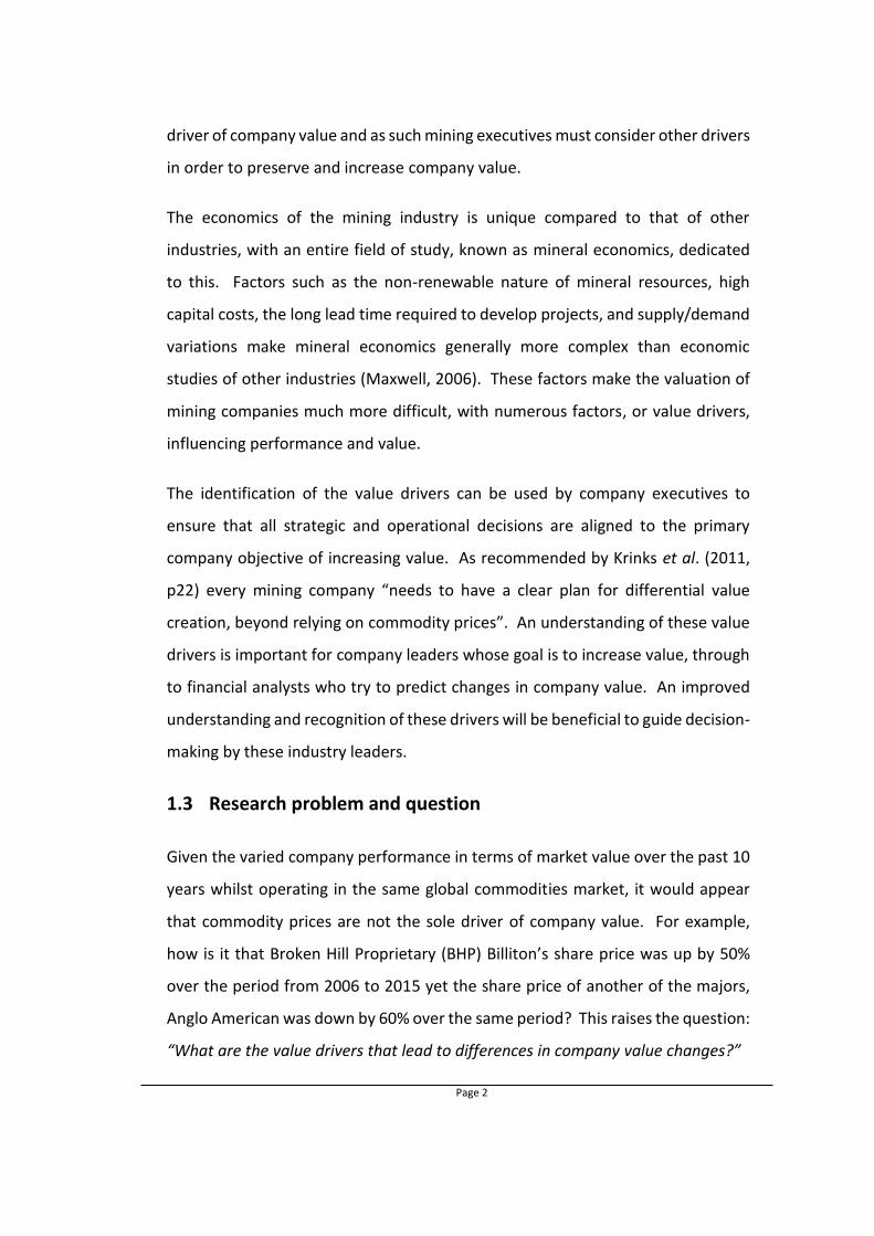
1.3 Research problem and question
Given the varied company performance in terms of market value over the past 10
years whilst operating in the same global commodities market, it would appear
that commodity prices are not the sole driver of company value. For example,
how is it that Broken Hill Proprietary (BHP) Billiton’s share price was up by 50%
over the period from 2006 to 2015 yet the share price of another of the majors,
Anglo American was down by 60% over the same period? This raises the question:
“What are the value drivers that lead to differences in company value changes?”

Page 3
1.4 Research objectives
This study analysed the hypothesis on whether the variable performance in
company value between four major mining companies, as measured by enterprise
value, can be traced to a number of key value drivers. This hypothesis was
explored by analysing company enterprise value over the 10 year period from
2006 to 2015, against identified key value drivers during the same period to
determine any patterns between market performance and the value drivers.
The objectives of this research study were to:
Review available literature on enterprise value to determine possible value
drivers;
Collect the relevant company performance and value driver data from
available company reports;
Develop indexed comparison of company value versus each of the value
drivers;
Analyse this data to identify any correlation and trends between potential
value drivers and company value;
Identify key drivers of company value over the period; and
Provide a recommendation on where companies should focus in order to
preserve and increase company value.
It is important to note that the objective of this project is not to do a specific
valuation of any of the mining stocks. Instead, it is to do a statistical analysis of
value drivers against indexed enterprise value to determine any trends between
value drivers and value. As such valuation techniques such as the discounted cash
flow, real option pricing, comparable transaction or other approaches were not
considered in this study.
Page 4
1.5 Research scope
The research study focused on four major international diversified mining
companies being, in alphabetical order, Anglo American Plc, BHP Billiton Ltd /
South 32, Rio Tinto Group and Companhia Vale do Rio Doce (CVRD-Vale). Whilst
Glencore and Xstrata could be considered, their 2013 merger makes it difficult to
analyse the pure value drivers to performance over this period, and thus they were
excluded as discussed in Section 1.6.
The period from 2006 to 2015 was selected as it represents a range of economic
conditions for a comprehensive analysis of mining companies. The period 2006 –
2008 represents a time when the mining boom saw mining companies making
extraordinary profits. This was followed by a brief, but drastic downturn with the
onset of the GFC, and subsequent rapid recovery during 2010 and 2011. Then
following this, the period 2011 to 2015 saw a steady downward trend in
commodity prices and increased pressure on mining companies to reduce
expenditure and react to these softer prices.
1.6 Selection and justification of mining companies
In order to identify any trends between value drivers and enterprise value, a range
of mining companies had to be selected and analysed. However, it is important to
note that within the mining industry two distinct sizes of companies exist, the
majors and the juniors. The difference between the two is very important for
company valuation, as outlined by Beattie (2016). The majors are traditionally well
capitalised with steady cash flows. As such, in theory, their enterprise value
should be relatively stable or experience steady growth. Juniors on the other
hand, tend to be speculative with hopes of a discovery of a feasible mineral
resource to boost returns. For this reason the drivers of value are much more
difficult to track, reliant on exploration with big risks and reward. Therefore, this

Page 5
research focused only on major mining companies which can be reliably evaluated
for differing performance due to different value drivers.
For the purpose of this report, major mining companies are defined as multiple
commodity, publically listed mining companies. For these major mining
companies, revenue is essentially a measure of sales, thus, by ranking companies
by revenue it was possible to select which companies have the biggest influence
on the global commodities market. As such, the companies selected should have
revenue which represents a major portion of the total worldwide commodity
sales.
According to Price Waterhouse Coopers (2007), for the 2006 calendar year the top
four mining companies accounted for nearly 43% of the total revenue and almost
47% of profit before interest and tax for the top 40 mining companies. These top
four companies included Anglo American plc, BHP Billiton Group, Rio Tinto Group
and CVRD-Vale with their contributions to revenue as shown in Table 1.1. It is
possible to increase the share of revenue and profit before interest and tax to
above 50% by including a fifth company, which was Xstrata plc.
Table 1.1: Top five mining companies by revenue - 2006 Source: Price Waterhouse Coopers (2007)
2006 (USD billion)
Total revenue 237.0
Anglo American PLC 33.1 14%
BHP Billiton group 32.8 14%
Rio Tinto group 22.5 9%
CVRD-Vale 19.7 9%
Xstrata 17.1 7%
Top 4 companies 109.3 46%
Top 5 companies 126.4 53%

Page 6
These five companies, at the time and historically, have been considered the
world’s major international mining companies and should represent a fair range
of data for performance analysis. However, this is just a snapshot as of 2006.
Over the eight year period following this, from 2006 to 2014, BHP Billiton, CVRD-
Vale, Rio Tinto and Xstrata have all remained within the top four revenue earners
of mining companies. Anglo American however has made a steady decline year-
on-year to be ranked twenty seventh by revenue as of 2015 (Price Waterhouse
Coppers, 2016). These 2006 top five companies by 2015 were ranked as per Table
1.2. As can be seen, whilst BHP Billiton and Rio Tinto have retained the top two
positions, the other companies have dropped significantly.
Table 1.2: Mining company ranking by revenue - 2015
Source: Price Waterhouse Coopers (2016)
2015 ranking (by revenue)
BHP Billiton 1st
Rio Tinto 2nd
Xstrata/Glencore 6th
CVRD-Vale 8th
Anglo American 27th
The other three positions for 2015 were filled by companies from three emerging
countries. These three companies are China Shenhua Energy Company Limited,
Coal India Limited and MMC Norilsk Nickel from Russia. The analysis of the value
drivers for these three companies for the period of 2006 to 2015 is much more
difficult as their financial details are not readily available in the public domain. As
such, the top five companies by revenue from 2006, all of which are international
publically listed traditional mining companies, were considered for this research
study.
In May 2013 Xstrata formally merged with Glencore, a Switzerland based
commodities trading company, to form the mining conglomerate Glencore

Page 7
Xstrata. At the time of the merger the new London listed company rivalled Rio
Tinto for size (Solly, 2013). Since this merger was towards the end of the period
of analysis for this research study, it is difficult to isolate this in terms of enterprise
value for the company. Whilst the other companies have all gone through smaller
mergers, acquisitions and sales during the period of analysis, none of them were
as significant as the Xstrata Glencore merger. As such, Xstrata was excluded from
this analysis.
Therefore, this research study was restricted to the analysis of the top four mining
companies by revenue as of 2006, these being Anglo American plc (referred
throughout as Anglo American), BHP Billiton Group (referred to as BHP Billiton),
Companhia Vale do Rio Doce (referred to as CVRD-Vale) and the Rio Tinto Group
(referred to as Rio Tinto).
1.7 Introduction to the selected major mining companies
This section of the report provides a brief overview and history of the four mining
companies selected for analysis. In many cases the history of the company is
important to understand changes in productivity and economic performance.
1.7.1 Anglo American plc
According to the company history by Anglo American (2016a), the company was
founded in 1917 by Sir Ernest Oppenheimer using a combination of capital from
sources in Britain and the United States, hence the name Anglo American. The
initial focus for the company was gold mining in the East Rand in South Africa. In
the 1920s the company broadened its commodity focus, through exploration for
platinum in South Africa and adding diamonds by becoming the largest single
shareholder of De Beers. Over the next 50 years the company expanded into coal,
copper, iron and a number of other products and services (Spector, 2012). In the
late 1960s and early 1970s the company expanded further out of the commodities
sector to include the steel and pulp/paper industry through acquisition of Scaw

Page 8
Metals and Mondi Group. Much of the investment in the non-mining sector was
as a result of restrictions in place due to South Africa’s Apartheid regime. In 1987
the company purchased a wine estate, Vergelegen, which it still owns at the time
of this research study.
By the end of Apartheid in 1994 the company was the world’s largest producer of
gold and platinum group metals, as well as a major producer of gold, diamonds,
copper, nickel, iron ore and coal. With operations worldwide, it was one of the
top three mining companies in the world. With the end of Apartheid removing
trade restrictions, the company began to sell-off many of its non-core businesses
and replaced them with other international mining opportunities.
By the early 2000s Anglo American was still very much a diversified mining
company, having changed its primary listing to the London Stock Exchange in 1999.
Over the next 10 years the company continued to expand with the following
transactions (Anglo American, 2016a):
2001 - Purchase of Shell Petroleum Company’s Australian coal asset;
2002 - Acquired the Los Bronces and El Soldado copper mines in Chile to
become Chile’s third largest copper producer;
2002 – Acquired a major stake in Kumba Resources South Africa, increasing
its exposure to iron ore;
2007 – Completely divested from gold through the formation and sale of
AngloGold Ashanti;
2007 – Sold off its Mondi Group, the paper and packaging business;
2007 – Made an initial investment in the Minas-Rio iron ore project in
Brazil;
2012 – Increased its stake in De Beers from 45% to 85%; and
2015 – Sold its stake in Lafarge Tarmac – a building materials company.

Page 9
The company has received significant criticism for its investment in the Minas Rio
Iron Ore Project in Brazil. Since its purchase in 2007 for $5.1bn, at close to the
peak of the iron ore boom, the total project cost was running well above $13bn in
2015 (Seccombe, 2015). This initial purchase, and subsequent project investment,
has weighed heavily on the company’s debt levels as is outlined later in this report.
In 2015 Anglo American was the worst performing stock on the Financial Times
Stock Exchange 100 Index (FTSE 100) dropping more than 73% for the year, only
slightly worse than Glencore’s 72% drop (Biesheuvel & Crowley, 2015). However,
for the first half of 2016 the share price recovered over half of those losses, as the
company promised to reduce debt via the sale of multiple assets and a focus on
three primary commodities – diamonds, platinum and copper. As of the end of
2015, the company’s revenue was split fairly evenly between five main
commodities being platinum, diamonds, coal, base metals (copper and nickel) and
iron ore with a very small portion from niobium phosphates and corporate
activities.
1.7.2 BHP Billiton Group
BHP Billiton was formed out of a 2001 merger between two small mining
companies, Broken Hill Proprietary Limited and Billiton, both with histories dating
back to the 1880s (BHP Billiton, 2016a). This merger formed the world’s largest
diversified resources company with operations in 20 countries and commodities
which include aluminium, coal, copper, ferro-alloys, iron ore, titanium, nickel,
diamonds and silver, as well as a large energy sector (Pederson, 2005). In 2005,
the merged company purchased WMC Resources, an Australian based copper,
gold and uranium major, adding uranium to its already diverse portfolio of
commodities. Then in late 2007, at the peak of the commodities boom, the
company announced plans to take over rival Rio Tinto. However, this did not
happen due to the onset of the GFC.

Page 10
From 2007 the company made a number of small purchases and sales, until in
2014 when it announced plans for a demerger of a number of operations to create
an independent metals company based on “a selection of its high-quality
aluminium, coal, manganese, nickel and silver assets” (BHP Billiton, 2014a, p1).
The company said the remaining assets would allow for a focus on the large, long-
life iron ore, copper, coal, petroleum and potash business. The spinoff company,
South 32, which formally listed on the Australian Stock Exchange (ASX), London
Stock Exchange (LSE) and the Johannesburg Stock Exchange (JSE) in May 2015, has
struggled with falling commodity prices, dropping by 50% on the ASX by the end
of 2015 and then recovering to the same listing price in September 2016. As this
demerger occurred during the period of this research study, South 32’s production
and performance was included in the analysis.
From 2015 the company has focused on a strategy to “own and operate large,
long-life, low-cost, expandable, upstream assets diversified by commodity,
geography and market” (BHP Billiton, 2016b, p1). As of the end of 2015,
approximately one-third of the company’s revenue was from iron ore, one quarter
each from petroleum (including potash) and copper and the remainder from coal
and other corporate activities.
1.7.3 Rio Tinto Group
According to the history of the company by Rio Tinto (2016b), the company was
formed in London in 1873 through the purchase of the rights to mine ancient
copper mines in southern Spain. In the 1920s the company started to diversify out
of Spain, with investment in copper mines in then Rhodesia, Africa. By the 1950s
the company had sold-off two-thirds of its interests in Spain and used these funds
to invest in bauxite in Australia. As such, in the 1960’s the company started to
build a large iron ore empire, which today makes it the world’s second largest iron
ore producer behind CVRD-Vale (Minerals Council of Australia, 2015). In 1983 the

Page 11
company added diamonds to its portfolio with the opening of the Argyle Diamond
Mine in Australia.
The company continued to grow and in the year 2000, right at the start of the
minerals boom, it undertook US$4 billion worth of acquisitions - primarily
Australian aluminium, iron ore, diamond and coal assets. This was further backed
up by the 2007 acquisition of Alcan, creating a world leader in aluminium
production. By the early 2010s the company was a major player in iron ore,
aluminium, copper, coal and diamonds. In 2015 the company received over 40%
of its revenue from iron ore, close to a quarter each from aluminium and
copper/coal (grouped together for reporting) and the remaining 10% from
diamonds and other minerals.
1.7.4 Companhia Vale do Rio Doce (CVRD-Vale)
According to Vale (2012a) which provided the history of the company, Companhia
Vale do Rio Doce, known then as CVRD, was founded in 1942 by the Brazilian
Federal Government, to form a state owned mining company. The company’s
initial focus was on iron ore, and by 1974 it was the world’s biggest exporter of
iron ore, a title it still holds at the time of writing this report. In 1997,
approximately 42% of the company was auctioned off as part of a partial
privatisation of the company. The focus on iron ore remained until the 2000’s
when the company started to diversify into other minerals. The largest of these
diversification moves was the 2006 purchase of the Canadian copper, nickel and
other metals producer Inco Limited.
In the following year, as part of its move from being a local iron ore miner to a
global diversified company, the group launched a rebranding to be known as Vale
rather than the traditional CVRD. In 2007 Vale entered the coal mining sector
through the purchase of AMCI Holdings Australia, and opened coal assets in
Mozambique. In 2012 the company added gold to its portfolio with the opening
Page 12
of the Salobo Mine in Brazil. By the end of 2013, after 70 years since formation,
the company had a presence in more than 35 countries with operations producing
all the major commodities, excluding diamonds, and was one of the top five mining
companies worldwide. In 2015 the company received close to 70% of its revenue
from ferrous metals, 20% from nickel and the remainder from copper, coal and
fertilisers.
1.8 Chapter conclusion and structure of the report
As the history of the four major mining companies included in this research report
shows, all are multi commodity, diversified international mining companies. Thus
they are appropriate for analysis of value drivers for differing company value
performance. Chapter 2 of this report provides a literature review of the theory
behind company value and valuation techniques. It also provides a review of
possible value drivers for mining companies.
Chapter 3 describes the research methodology used, identifying the value drivers
to be analysed and explaining the data collection and analysis process. As all data
was collected from publically available company financial and production reports,
the different values extracted from these reports are explained. Any calculations
required to determine the value drivers are also detailed.
Chapter 4 presents and analyses the data, first by showing the variation in
company performance over the 10 year period, and then presenting each of the
different potential value drivers for each company. These are primarily presented
in graphical form with any required detail provided in the text. Statistical
correlation analysis is also undertaken on the valuation multiples and the capital
efficiency drivers, to determine the correlation between these and enterprise
value. This analysis identifies the potential value drivers which significantly
influence and are key to company value performance.

Page 13
Chapter 5 summarises the results on the identified key value drivers. Conclusions
derived from the data analysis and key value drivers are also provided. Finally, this
chapter provides a number of recommendations, tying the results back to the
objectives and identify how companies should consider these drivers when
targeting company value.

Page 14
2 LITERATURE REVIEW
2.1 Chapter overview
This chapter provides background information on the research topic. Much has
been written around the economic theory and practice of company valuation. As
such the concept of company value and valuation is introduced, to determine the
most appropriate value metric for this study. Mineral asset valuation is also
introduced to understand its relevance in comparison to company valuation. Then
the different metrics and techniques for market valuation are reviewed and
discussed to identify the different possible value drivers which influence company
value.
2.2 Overview of company value, value drivers and valuation
approaches
Value is defined as the material or monetary worth of something (Oxford
Dictionary, 2016). When dealing with company value, this can include not only
the monetary value of the business but also shareholder value, employee value
and societal value. However, in terms of this study, value and valuation are linked
to the monetary value of the business. “Value is a particularly helpful measure of
performance because it takes into account the long-term interest of all
stakeholders in a company, not just the shareholders” (Koller et al., 2005, p3). As
such, changes in the value of a company over time can be used as a measure of
whether a company has performed positively or negatively. The process to
calculate this value is known as company valuation defined by Investopedia
(2016a, p1) as a “process of determining the economic value of a business or
company”. Whilst the most common use of valuation is the buying and selling of
operations/companies, as identified by Fernàndez (2007) company valuation can
also be used to identify and stratify sources of economic value creation and

Page 15
destruction. In other words the purpose is to identify the value drivers for a
company.
L.E.K Consulting (nd, p2) suggested that “by focusing on value drivers,
management can prioritize the specific activities that will affect performance in
each area”. However, for many companies the challenge is to understand which
value drivers have the biggest influence on company value. Similarly, whilst some
value drivers may have a big impact on value, management may have little
influence on these and not be able to change them. The different value drivers,
based on value impact and management influence should therefore be ranked and
considered as per Figure 2.1.
Figure 2.1 : Value driver matrix for prioritising value drivers Source: L.E.K. Consulting (nd)
Page 16
From this figure it can be seen that management must focus on and manage the
drivers with highest impact on value, giving less priority to those which are of
lower impact or which they have less influence over. These high priority drivers
should be considered key value drivers and should form part of management’s key
performance indicators (KPI’s). As such, this study focused on determining those
value drivers which have the highest value impact
One important distinction that must be made which is specific to mining
companies is company valuation versus mineral asset valuation. Mineral asset
valuation is used to determine the value of a specific resource or operation and
are used by mining companies to ascertain the value of their assets for impairment
test, annual audits or investor corporate communications (Deloitte, 2016a).
Njowa et al. (2013) described ongoing work from the late 2000’s to develop a
globally accepted mineral asset valuation template, rather than having individual
regional codes. This is in an attempt to harmonise the three current major codes
being:
The Code for the Technical Assessment and Valuation of Mineral and
Petroleum Assets and Securities for Independent Expert Reports (The
VALMIN Code) for Australasia;
The Standards and Guidelines for Valuation of Mineral Properties (The
CIMVAL Code) for Canada; and
The South African Code for the Reporting of Mineral Asset Valuation (The
SAMVAL Code, 2016) for South Africa.
Each of these codes provides guidelines for the valuation of mineral assets
depending on the stage of development of the project. As an example SAMVAL
(2016) sets out the minimum standards and guidelines for reporting of mineral
asset valuations in South Africa. This paper suggests that in the extractive
industries, value is usually derived from an assessment of the intrinsic value of the
unique technical characteristics of the asset. As such, it suggests that of three

Page 17
recommended valuation approaches, being income, market and cost approaches,
two valuation approaches should be used to assess the value of a mineral asset.
However, as this research is reviewing changes to company value rather than
resource or asset value, different mineral valuation techniques were not reviewed.
Instead this research focussed on company value, with a range of valuation
techniques available.
Accurate determination of the economic value of a company is difficult, with the
calculation based on both buyer and seller perception of the company. For this
reason a number of different valuation approaches have been developed, each
with its own purpose and relevance, depending on the requirements of the
valuation. NAVCA (2008) split the commonly used company valuation approaches
into three categories being asset based approach, income approach and market
approach. These three primary approaches each contain a number of different
valuation methods.
2.2.1 Asset based valuation
Asset based valuation considers that the total value of a company can be
determined by the difference between the company’s assets and its liabilities. It
is also referred to as balance sheet based valuation, since the balance sheet
contains information on the company’s assets and liabilities. In consideration of
asset based valuation techniques, Fernàndez (2007) explained that whilst
traditionally, company value lies in its balance sheet, generally the equity’s asset
value has little bearing on its market value. This is because this approach does not
take into account the company’s earnings, current industry situation and future
potential earnings, as these do not appear on the balance sheet.
This is particularly relevant for mining companies where the primary assets are the
individual mineral resources and mineral reserves which the company has title to.
The market value of these, as determined by the mineral asset valuation

Page 18
previously discussed, will not appear on the company’s balance sheet. As such this
asset based approach is not appropriate for mining company valuation.
2.2.2 Income based valuation
Income based valuation is based on the company’s expected income streams
rather than the balance sheet. This approach attempts to calculate all anticipated
future earnings and economic benefits into a single amount. This includes metrics
such as net present value, discounted cash flow and other future earnings
valuation calculations. In reviewing the income based valuations, Steiger (2008)
suggested that whilst these methods are a powerful tool for determining company
value for capital budgeting, this approach is very vulnerable to changes in the
underlying assumptions. Again, this is particularly relevant for the valuation of
mining companies, where the calculation of future income streams is dependent
on forecasting commodity prices, something which is a potential source of
variability. The income approach is often used for the valuation of individual
mineral assets, particularly as part of feasibility studies. However, to combine
these individual valuations into a company valuation is difficult and as such not
appropriate for this study.
2.2.3 Market based valuation
Market based valuation uses the concept that the value of a business is calculated
by determining what an investor would be willing to pay for the company. For
non-publically listed companies, or for the valuation of individual mining projects,
this is done using market comparable methods. However SAMVAL (2016, p10),
which provides guidelines on the valuation of a mineral asset, suggests that “the
application of certain logic in Mineral Asset Valuation, such as ‘gross in-situ value’
simply determined from the product of the estimate of mineral content and
commodity price(s), is considered unacceptable and inappropriate”. As such it is
often difficult to determine the properties used for value calculation. Ellis (2016)

Page 19
researched how this comparable method can be used for mineral property
valuation. In doing so, the research suggested that for mineral property interests
there are a number of constraints in this method, specifically around identifying
suitable properties for comparison. As such this was not considered as a valuation
method for this study.
For many non-public (or private) and publically listed companies the market based
valuation approaches involve the market capitalisation of the company. Whereas
the asset and income based approaches attempt to calculate the intrinsic value of
a company and can vary based on the input assumptions, the market valuation
approaches give the value from the willing buyer, willing seller principle and
requires that the monetary value obtainable from the sale of the company is
determined as if in an arm’s-length transaction (SAMVAL, 2016). This market value
includes all underlying economic fundamentals, with investors considering the
long-term potential of stocks to determine its value (Koller et al, 2005). As this
research study is focused on analysing changes to company value over time, the
more simplistic market valuation approach is therefore used in this study. This
approach is more transparent, allowing the value estimated for a mining company
to be benchmarked against other companies (Roberts, 2006).
The market value of a company is measured in two main ways. The simplest way
is to calculate its market capitalisation, which is a multiple of the share price and
the total number of outstanding shares. However, this calculation omits a number
of important aspects which contribute to the overall value of a company, including
debt, cash and cash equivalents. Bhullar & Bhatnagar (2013) suggested that a
more appropriate measure of company value is enterprise value (EV), which
provides a measure of the real market value of a firm as a whole business. As
such, EV was used in this research study as the measure of company value and
performance over the period under review.
Page 20
2.3 Enterprise value and its potential drivers
Enterprise value is commonly defined as the equity value plus total debt, preferred
stock and minority interest, minus cash and cash equivalents (Investopedia,
2016b). An alternate calculation for EV is the sum of the company’s market
capitalisation and its net debt. This is essentially the theoretical takeover price to
buy out an entire public company, giving a much clearer picture of real value
compared to market capitalisation.
The equity value of a company is calculated from its market capitalisation. This is
the value of the company’s outstanding or issued shares which is calculated by
multiplying the current share price by the number of outstanding shares. Net
debt is the total short and long term debt, minus any cash and cash equivalents.
The reason for including any cash and cash equivalents is that these could
theoretically be offset against any debt commitments. These calculations were
used to calculate the EV of the selected companies, at different points in time,
which represents changes in company value.
There are several factors which drive the EV of mining companies. Bhullar &
Bhatnagar (2013) provided similar guidelines, suggesting that EV can be improved
by three methods: increasing sales, reducing costs and reducing capital lockup.
Supporting this, Deloitte (2012) suggested that the most common value drivers
can be depicted as drivers of shareholder value as shown in Figure 2.2.

Page 21
Figure 2.2 : High level shareholder value map Source: Deloitte (2012)
Based on these guidelines, a number of different metrics were selected for
analysis as drivers of company value. Revenue growth was analysed in terms of
volume and price. Operating margin was analysed using valuation multiples which
“attempt to capture many of a firm’s operating and financial characteristics”
(Macabacus, 2016, p1). This is particularly important for mining companies, which
following the boom times experienced reduced profits as they struggled to get
escalating costs under control. Asset efficiency, referred to in this report as capital
efficiency, analyses how well a company uses its debt and equity portions to add
company value. Analysis of expectations, in terms of company strengths and
external factors, is much more difficult to correlate to EV as single metrics. As
such, specific analysis of this was excluded from this study. However, where
relevant links to expectations were identified and are discussed in this report.
2.3.1 Revenue drivers
The basic calculation of revenue is price multiplied by quantity of product sold
(volume). For the mining industry, this is commodity production output multiplied
by commodity price. Thus, the two potential drivers for revenue for mining
companies is commodity price and production output.
Page 22
Commodity price
The most obvious value driver of a mining stock is the price of the commodities
produced, particularly for established mining companies (Maverick, 2015).
However, Baurens (2010) identified that the valuation of mining companies is
complicated because of the cyclical nature of commodity prices and that
commodity companies are mostly price takers. This is because most minerals,
excluding as an example diamonds, are fungible meaning that they can be
mutually substituted. This means that unlike most industries where producers can
influence the price of their products by changing quality or output, mineral
commodity prices are dictated in the open market. As such the resulting valuation
varies depending on where in the price cycle that company’s output is.
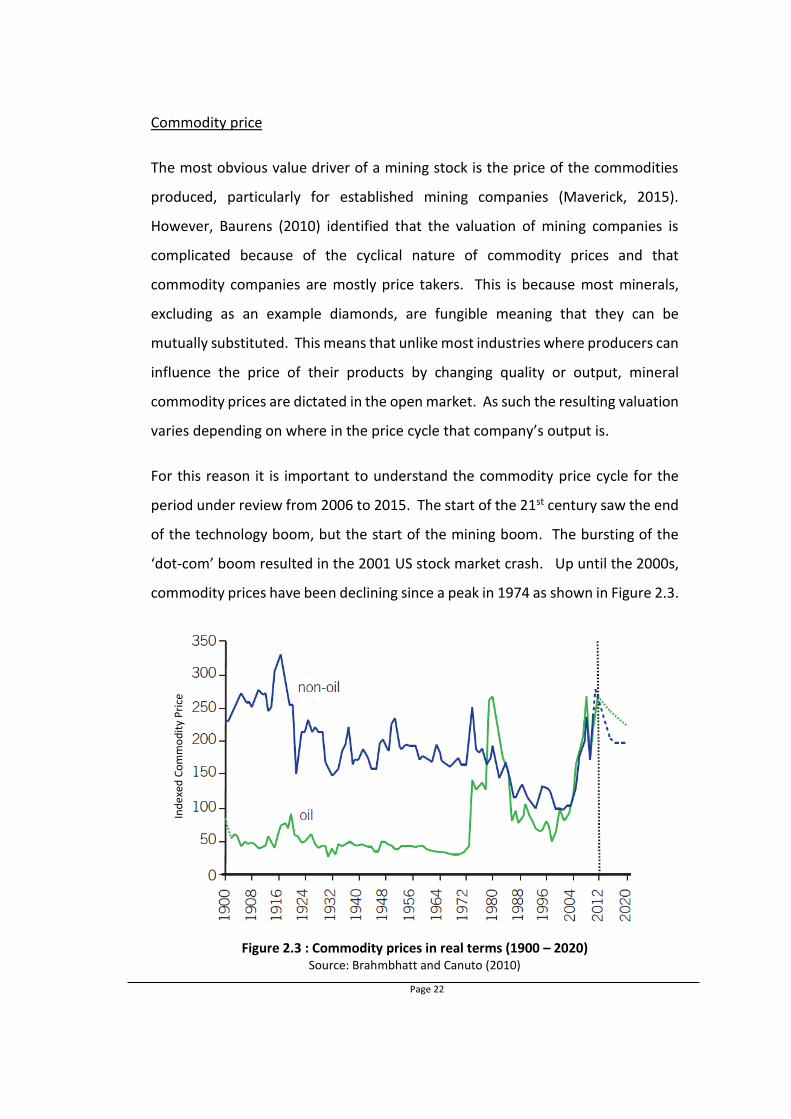
For this reason it is important to understand the commodity price cycle for the
period under review from 2006 to 2015. The start of the 21st century saw the end
of the technology boom, but the start of the mining boom. The bursting of the
‘dot-com’ boom resulted in the 2001 US stock market crash. Up until the 2000s,
commodity prices have been declining since a peak in 1974 as shown in Figure 2.3.
Figure 2.3 : Commodity prices in real terms (1900 – 2020) Source: Brahmbhatt and Canuto (2010)
Ind
exe
d C
om
mo
dit
y P
rice

Page 23
As of 2000 non-oil commodity prices were at their lowest levels in real terms for
the entire century. However, this was all to change very quickly, with the rapid
urbanisation and industrialisation of emerging economies, particularly those of
China and India. This increased demand for most commodities, linked with limited
supply, resulted in extraordinary increases in commodity prices. As can be seen
in Figure 2.3, from the start of the boom in 2001 to the onset of the GFC in late
2008, commodity prices increased by over 250%.
Thus by 2006, the start of the analysis period for this study, the boom in
commodity prices was well underway. Mining companies were continuously
beating previous year revenue and profit outputs, and paying out growing
dividends to investors. The majors were constantly on the lookout for
opportunities to expand and increase production, in many cases with little
consideration of the costs of such expansions. Price Waterhouse Coopers
annually produce a mining publication which reviews global trends of the mining
industry for the previous year. This is primarily done by reviewing the
performance of the top 40 mining companies and gives a very good picture of the
changing industry and commodity cycles over the period. The titles of these
reports convey the sentiment of the period with the 2006 publication titled “Let
the good times roll” (Price Waterhouse Coopers, 2006). In 2006, they reported
that net profits for the top 40 mining companies were 1423% higher than the 2002
equivalent (Price Waterhouse Coopers, 2007).
Nevertheless this was all about to change drastically in 2008, with the onset of the
GFC. In April 2008 the US government had to bail out two major financial
institutions as a result of a sub-prime mortgage crisis. “Like a pack of dominoes,
most banks with large sub-prime exposures joined the solvency and liquidity
fracas” (Baxter, 2009, p106). As a result of this, for some commodities in a space
of a couple of months, prices crashed to close to pre-boom times. Figure 2.4 shows
this crash charting indexed average annual commodity prices with the spot price
as of the end of 2008 shown at the end. As a result, in 2008 the market

Page 24
capitalisation of the top 40 mining companies decreased by 62% (Price
Waterhouse Coopers, 2009).
Figure 2.4 : Commodity prices indexed to 2003 Source: Price Waterhouse Coopers (2009)
In late 2009 and early 2010, the price of most commodities recovered to above
pre-GFC levels and as such most companies started to recover to similar levels.
This was relatively short lived, with the price of most commodities on a steady
decline since the start of 2011 to the end of 2015, as shown in Figure 2.5. As a
result, these years have been tough for mining companies with reduced demand
pushing prices down and companies battling with the legacy of escalating cost
bases from the boom times.
Figure 2.5 : Changes in key commodity prices since January 2011 Source: Ernst & Young (2015)
Ind
exe
d P
rice
(2
00
3 b
ase)
In
de
xed
Pri
ce

Page 25
Given the variable performance between mining companies, commodity price
cannot be the sole driver of mining company value. Widespread evidence exists
to show that the rise and fall of company value is not just linked to commodity
prices. For example, the market capitalisation of the top 40 mining companies
dropped by 37% in 2015, which is disproportionately greater than that of
commodity prices (Price Waterhouse Coopers, 2016). The same is apparent in
times of rising prices, for example for the first 6 months of 2016, the gold bullion
price rose by 27.7% yet the gold equities, as displayed by the FTSE Gold Mine
Index, increased by 110.4% (FTSE Russell, 2016). Given this, there are obviously
other factors that affect company value.
In most cases a mining company’s revenue is as volatile as the price of the
commodities it is producing. This is because revenue is a direct multiple of price
and production output. As such both the commodity price and the production
output determine company revenue and in combination were included as part of
the analysis.
Production output
Whilst companies have very little control over commodity prices, they can
influence how much they produce of each commodity. As commodity prices
started to increase in the early 2000s, the main focus for mining CEO’s moved from
cutting costs and operational efficiency to “mine supply and maximising
production” (Price Waterhouse Coopers, 2006, p3). However, the mining industry
is unique to other industries in that mining projects have long lead times. As such
companies cannot react to increased demand by quickly bringing on additional
capacity. Consequently, the production output across the industry has been
relatively flat. Table 2.1 shows the annual change in production output for the top
40 mining companies from 2007 to 2011.

Page 26
Table 2.1: Year on year change in production output – top 40 mining companies
Sources: Price Waterhouse Coopers (2009, 2010, 2011, 2012)
2007 2008 2009 2010 2011 Average
Gold 9% -8% 7% 2% 9% 4%
Platinum -9% 0% -4% 0% 2% -2%
Copper 4% 1% 0% -4% 16% 3%
Zinc 11% 2% 9% 0% -10% 2%
Coal 6% 4% -2% 1% -1% 2%
Iron Ore 7% 7% -3% 16% 6% 7%
Nickel 8% -1% -11% 4% 13% 3%
As can be seen whilst in some years there are relatively large jumps in production
output, in general output is relatively flat for the mining industry. Thus, the
primary way mining companies increase production output is through acquisition
of other companies and operations. As such, changes in production output for
each of the major mining companies was analysed as this affects total revenue of
the group.
2.3.2 Valuation multiples
Krinks et al. (2011) analysed the performance of 37 top mining companies to
understand where they created greatest returns for shareholders from 1999 to
2009. Their research study indicated that increases in valuation multiples was a
major contributor to strong shareholder returns. Their study included valuation
multiples of earnings before interest, tax, depreciation and amortisation (EBITDA)
multiple and EBITDA margin. The EBITDA multiple is defined as EV divided by
EBITDA. Bhullar & Bhatnagar (2013) suggested that EBITDA multiple is a preferred
valuation multiple to price on equity (P/E) as it considers debt and cash position,
but excludes potential tax differences. Loughran & Wellman (2010) provided
evidence on the link between enterprise multiples, which are valuation multiples
and stock returns, and as such should be linked to company performance.

Page 27
The second valuation multiple, EBITDA margin, is the EBITDA divided by total
revenue. This shows what portion of revenue is earnings and what portion is
operating expenses. Essentially this measure can be used to analyse which
companies have managed to keep costs in line with changes in revenue and which
have been most affected by escalating costs. In 2012 the net profit of the top 40
mining companies was down by 49% on the previous year (Price Waterhouse
Coopers, 2013). Most companies bulked up when prices were high, focusing on
expansion at all costs, and as softer commodity prices hit, the high costs remained
eroding operating profits. Price Waterhouse Cooper (2015) described the
importance of cost reduction for company value, highlighting how many
companies lost cost efficiency, which is potentially destroying company value.
2.3.3 Capital management and efficiency
Capital management and efficiency can be defined as “the prudent management
of the capital required to support a business and the use of the resulting free cash
flows” (Krinks et al, 2011, p19). The authors further said that a large percentage
of the total shareholder returns for mining companies from 1999 to 2009 can be
attributed to effective and efficient capital management. Further to this, Deloitte
(2016b) provided details of the top 10 issues facing mining companies going
forward. One of the issues they discussed is industry debt burdens, which had
“spiralled out of control” having a major effect on the value of a company. By
2015, net debt ratios for the top 40 mining companies had risen to the highest
levels since the early 2000s and leverage was increasingly stretching the balance
sheets of many of the major mining houses (Ernst & Young, 2015). Whilst this is
an industry-wide issue, the extent of the issue varies significantly among
companies.
There are three common measures of capital efficiency being gearing ratio, net
debt to EBITDA and return on capital employed (ROCE). Gearing ratio is a measure
of a portion of the company’s assets (debt plus equity) which is debt. Examining

Page 28
this can provide an indication of the company’s financial strength, gauging the
capacity of corporates to absorb unexpected financial shocks (Ernst & Young,
2015). In general, if the gearing ratio is too high, it is a sign that a company may
be in financial distress and unable to pay debtors. Increasing gearing means the
financial risk associated with that company is also increasing.
The second capital management measure which is commonly used, and suggested
by Price Waterhouse Coopers (2016) as a convent applied by lenders is the net
debt to EBITDA. The same report suggested that ratios above four should cause
alarm to management and investors and as a benchmark the 2014 and 2015
averages across the top 40 mining companies were 1.52 and 2.46, respectively.
Net debt to EBITDA is an important measure as it shows the company’s ability to
pay back its debt. The higher the number, the more difficult it could be for the
company to pay off its debt, or be able to take on any additional debt required to
grow the business. As this figure is essentially a measure of how many years
EBITDA is required to pay off the company’s debt, this value must only be reviewed
on an annual year-end basis. As can be seen in Figure 2.6, which shows the above
measures for 88 listed mining companies, both of these values increased
significantly over the 15 year period from 2000 to 2014, potentially indicating a
major driver to company value over the period.
Figure 2.6 : Growing net debt in the mining industry – analysis of 88 listed mining companies
Source: Ernst & Young (2015)

Page 29
The third capital management value driver is ROCE. ROCE is a measure of the
company’s profitability compared to the capital employed to achieve this profit.
This is calculated by dividing the earnings before interest and tax (EBIT) by the
capital employed. The capital employed is commonly defined as the total assets
less the current liabilities. The higher the ROCE, the more efficient the company’s
use of available capital. It has been proven that the market rewards firms that can
get good returns on the capital they employ in their business, by valuing them at
a higher premium than their peers (Pattabiraman, 2013). ROCE is particularly
useful when comparing performance of companies in capital intensive industries
(Damodaran, 2007), something which the mining industry most definitely is. As a
benchmark for the mining industry, when Mark Cutifani joined Anglo American as
the CEO in 2013 he committed to achieving a ROCE of 15%, however with declining
commodity prices this target has slipped to a range between 5 – 15% between
2013 and 2016 (Wilson, 2016).
2.4 Chapter summary
This chapter has introduced the theory of company value. In order to determine
the company value a number of different valuation approaches are used including
the asset based approach, income approach and market approach. For the
purpose of this study the market based approach was considered the most
appropriate because of its limited reliance on input assumptions and its suitability
for comparing companies. Within this approach, existing literature suggests that
the most appropriate measure of company value is EV. Research also shows that
sales, costs and capital lockup are the main drivers of EV. These can be reclassified
into three main categories: revenue drivers, valuation multiples and capital
management and efficiency drivers. The main drivers of revenue were identified
as commodity price and production output. EBITDA multiple and EBITDA margin
are the two main valuation multiple drivers. Finally, gearing ratio, net debt to
EBITDA and ROCE are the main capital efficiency drivers. All of these drivers

Page 30
ultimately influence the EV of companies and were therefore selected as the value
drivers for this research study.

Page 31
3 RESEARCH METHOD
3.1 Chapter overview
This chapter discusses the research methods and analytical techniques used. The
data required to calculate EV and identified potential value drivers was obtained
from the public domain using company annual reports, half yearly reports and
quarterly production reports. Where the required values were not directly
reported they were estimated from available data. All measures were indexed
back to the 31st December 2005. The final date for analysis was the 31st December
2015 which represents a 10 year period and the position of the company as of the
start of 2016.
3.2 Data that was analysed and its sources
3.2.1 Enterprise value
As mentioned in the literature review, EV was used as the measure of company
value for this study. EV was not specifically reported in the annual financials by
any of the companies, so it was calculated from reported metrics. As previously
defined, EV can be calculated as net debt plus market capitalisation. Net debt was
reported by some companies, but in cases where it was not reported it was
calculated as the sum of both short and long term debt minus cash and cash
equivalents. Market capitalisation is the current share price multiplied by the
number of issued shares at the end of the period. The current share price as of
the close of each period was sourced from Yahoo Finance for each company
(Yahoo Finance, 2016a – d). The total number of shares issued and outstanding is
reported as part of the changes in stockholders equity in both annual and semi-
annual reports. For all companies the share prices from the primary listing was
used, being:

Page 32
Anglo American - London Stock Exchange;
BHP Billiton - Australian Stock Exchange;
Rio Tinto - London Stock Exchange; and
CVRD-Vale - New York Stock Exchange.
As the reporting currency for all companies is United States Dollars (USD), those
stocks that are reported in Great British Pounds (GBP) and Australian Dollars (AUD)
were converted to USD using the month average exchange rate for that currency.
These exchange rates were sourced on a monthly average from FXtop (2016) for
the period from January 2006 to December 2015. EV was calculated on a 6 month
interval and indexed back to the 31st December 2005.
Whilst share price is one of the main derivatives of EV, specific analysis of the
drivers of share price were not included in this study. Instead the focus was on
the main economic drivers of EV, of which share price is a subset.
3.2.2 Production output
The two primary drivers which were analysed for their effect on revenue was
production output and commodity price. An increase or decrease of production
output across all commodities, should show the growth or contraction of a
company respectively. In order to analyse this, the quarterly production output
for each of the primary commodities segments was indexed to the quarterly
production for the last quarter of 2005. This was compared to the indexed EV for
the same period, in order to identify trends. Thus, if a company is producing seven
main commodities in Quarter 4 (Q4) 2005, then the indexed output for the start
of the analysis is seven. Each commodity is then indexed quarter on quarter back
to Q4 2005 output and plotted on a stacked area graph. A hypothetical example
of this calculation is shown in Table 3.1 and then plotted in Figure 3.1.
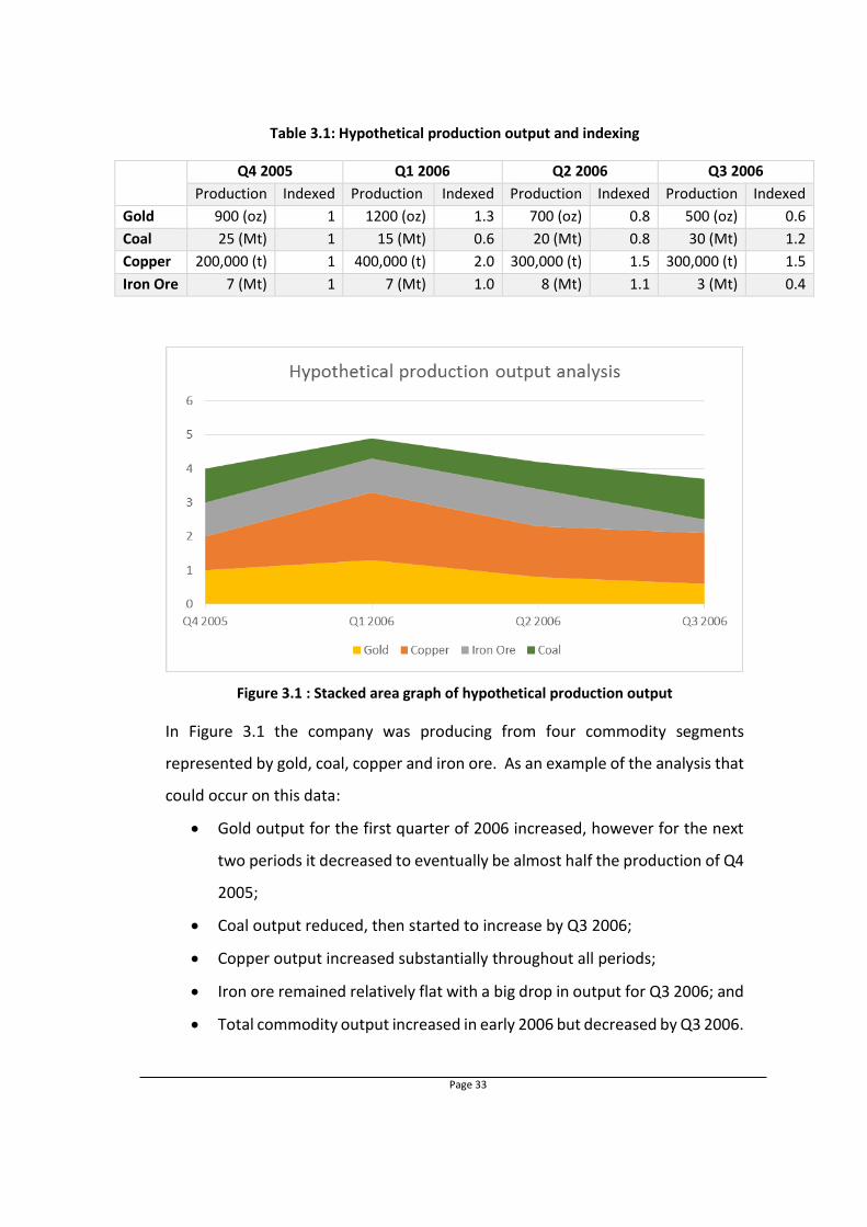
Page 33
Table 3.1: Hypothetical production output and indexing
Q4 2005 Q1 2006 Q2 2006 Q3 2006
Production Indexed Production Indexed Production Indexed Production Indexed
Gold 900 (oz) 1 1200 (oz) 1.3 700 (oz) 0.8 500 (oz) 0.6
Coal 25 (Mt) 1 15 (Mt) 0.6 20 (Mt) 0.8 30 (Mt) 1.2
Copper 200,000 (t) 1 400,000 (t) 2.0 300,000 (t) 1.5 300,000 (t) 1.5
Iron Ore 7 (Mt) 1 7 (Mt) 1.0 8 (Mt) 1.1 3 (Mt) 0.4
Figure 3.1 : Stacked area graph of hypothetical production output
In Figure 3.1 the company was producing from four commodity segments
represented by gold, coal, copper and iron ore. As an example of the analysis that
could occur on this data:
Gold output for the first quarter of 2006 increased, however for the next
two periods it decreased to eventually be almost half the production of Q4
2005;
Coal output reduced, then started to increase by Q3 2006;
Copper output increased substantially throughout all periods;
Iron ore remained relatively flat with a big drop in output for Q3 2006; and
Total commodity output increased in early 2006 but decreased by Q3 2006.

Page 34
This trend was then plotted against EV to see if changes in production output
drove company value. In order to consider both commodity price and production
output for each of the companies, both were indexed to Q4 2005 in order to
analyse any trends. However, in the case of CVRD-Vale, which expanded its
business to include additional commodity segments after 2005, indexing all
production output back to Q4 2005 was not possible. Thus it was indexed to the
first quarter (Q1, 2010) where it produced the full range of commodity segments.
The same analysis to EV was done.
The production per commodity for each company was available from the quarterly
production reports. Since the analysis of production output and commodity prices
starts with the revenue contribution for each commodity from 2005, commodities
were grouped together as per the company segments. Appendix 7.1 to Appendix
7.4 provide a summary of how each company has broken down various
commodities into segments. As some segments include a basket of different
commodities, the primary commodity or commodity which contributed the most
to segment revenue was selected for production and pricing analysis. Where no
commodity is produced, for example in the “other” segment, no production
analysis was done. Table 3.2 summarises the different segments for each
company, detailing the primary commodity, which was analysed for changes in
production output.
All production values were indexed back to the Q4 2005 output. However, to
ensure that this quarter was not abnormal and did not misrepresent the changes
in production output, the total production for 2005 for each commodity was
divided by four to get the average quarterly production for 2005.

Page 35
Table 3.2 : Summary of primary commodity analysed per company sector
Company Segment Primary commodity analysed
Anglo American
Platinum Refined platinum
Gold Gold
Diamonds Diamonds
Coal Total coal
Copper Copper
Nickel, niobium & mineral sands Nickel
Iron ore & manganese Total iron ore including lump and fines
Other mining, industrial & corporate
No analysis
BHP Billiton
Petroleum & potash Total petroleum
Aluminium, manganese & nickel Aluminium
Base metals Copper
Diamonds and speciality productions
Diamonds
Iron ore Iron ore
Metallurgical coal Metallurgical coal
Energy coal Energy (thermal) coal
Rio Tinto
Aluminium Aluminium
Iron ore Iron ore
Diamonds & industrial minerals Titanium dioxide
Copper Copper
Energy Thermal coal
CVRD-Vale
Ferrous metals Iron ore
Coal Thermal coal
Base metals Nickel
Copper Copper
Fertilizers Phosphate rock
Aluminium Bauxite
Logistics & others No analysis
3.2.3 Commodity prices
The second driver for revenue alongside production is the commodity price. The
specific commodity price for each of the company segments is analysed in the
revenue analysis. A more general analysis, using the trends of all the major
commodities was undertaken to determine if there was any link to EV. This looked
at the different baskets of commodities, all indexed back to the average price in
2005. The majority of commodity prices were collected from the World Bank

Page 36
commodity price “pink sheet” (World Bank, 2016). This data file included prices
for the following:
Copper –$/metric tonne;
Nickel - $/metric tonne;
Aluminium - $/metric tonne;
Platinum - $/troy ounce;
Gold - $/troy ounce;
Iron ore - $/dry metric tonne unit (dmtu). The cost and freight (cfr) price
was used which means that the seller arranges for sea carriage of the
product to the required port. Since indexed pricing is being used, then this
price is suitable for all companies;
Phosphate rock - $/metric tonne;
Thermal coal – $/metric tonne. Two different prices are provided for
thermal coal being Australia and South Africa. The Australian price is a free
on board (FOB) price to Newcastle & Port Kembla. For South Africa it is
FOB to Richards Bay Coal Terminal (RBCT). The Australian coal is of a
slightly higher energy rating and as such attracts a slightly higher price.
Both prices track fairly closely and since the four companies analysed are
exposed more to Australian production, the Australian thermal coal price
was used; and
Crude Oil - $/barrel ($/bbl). As reported by the World Bank the price is the
equally weighted average of crude oil Brent, crude oil Dubai and crude oil
US West Texas Intermediate (WTI).
The World Bank only reports thermal coal prices however as many of the mining
companies also produce metallurgical/coking coal this price was also required for
the analysis. Since the majority of the production of metallurgical/coking coal is
from Australia, the hard coking coal (HCC) spot FOB Australia price was used. This
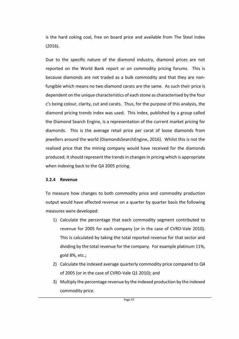
Page 37
is the hard coking coal, free on board price and available from The Steel Index
(2016).
Due to the specific nature of the diamond industry, diamond prices are not
reported on the World Bank report or on commodity pricing forums. This is
because diamonds are not traded as a bulk commodity and that they are non-
fungible which means no two diamond carats are the same. As such their price is
dependent on the unique characteristics of each stone as characterised by the four
c’s being colour, clarity, cut and carats. Thus, for the purpose of this analysis, the
diamond pricing trends index was used. This index, published by a group called
the Diamond Search Engine, is a representation of the current market pricing for
diamonds. This is the average retail price per carat of loose diamonds from
jewellers around the world (DiamondsSearchEngine, 2016). Whilst this is not the
realised price that the mining company would have received for the diamonds
produced, it should represent the trends in changes in pricing which is appropriate
when indexing back to the Q4 2005 pricing.
3.2.4 Revenue
To measure how changes to both commodity price and commodity production
output would have affected revenue on a quarter by quarter basis the following
measures were developed:
1) Calculate the percentage that each commodity segment contributed to
revenue for 2005 for each company (or in the case of CVRD-Vale 2010).
This is calculated by taking the total reported revenue for that sector and
dividing by the total revenue for the company. For example platinum 11%,
gold 8%, etc.;
2) Calculate the indexed average quarterly commodity price compared to Q4
of 2005 (or in the case of CVRD-Vale Q1 2010); and
3) Multiply the percentage revenue by the indexed production by the indexed
commodity price.

Page 38
This output represents the estimated changes to revenue through changes in
commodity price and production. A hypothetical example of this calculation, using
hypothetical data, is shown in Table 3.3 and Table 3.4.
Table 3.3 : Hypothetical price and production data
2005 Revenue
2005 Q4 Commodity
price
2006 Q1 Commodity
price
2005 Q4 Production
2006 Q1 Production
Gold $US25M $ 478 $ 591 1,500 1,500
Copper $US25M $ 1.90 $ 2.76 150,000 100,000
Platinum $US25M $ 944 $ 1,107 700 700
Iron Ore $US25M $ 69 $ 68 7.8 9.5
Table 3.4 : Hypothetical commodity price, production and revenue change
% Revenue contribution
2006 Q1 Indexed commodity price
2006 Q1 Indexed production
2006 Q1 Theoretical
indexed revenue
Gold 25% 1.24 1.00 31%
Copper 25% 1.45 0.67 24%
Platinum 25% 1.17 1.00 29%
Iron Ore 25% 0.99 1.22 30%
Total 100% 115%
As can be seen in Figure 3.2 through the hypothetical example above, the total
revenue produced by the company should have increased. Copper, which had the
greatest increase in price actually decreased in revenue due to reduced
production. Iron ore had increased revenue however this was due to production
rather than commodity price. The company could have had a much higher
revenue by increasing production in those commodities where the price increased
the most (gold and copper) and focused less on the commodities where the price
remained relatively flat or decreased (iron ore).

Page 39
Figure 3.2 : Hypothetical commodity price and production analysis
Where a company had significant revenue contribution from non-commodity
sectors, for example CVRD-Vale’s logistics business, the annual percentage
contribution to revenue was extracted from the annual financial reports and this
figure was used for each quarter of the year.
3.2.5 Valuation multiples
The two valuation multiples which were analysed were EBITDA multiple and
EBITDA margin. EBITDA was reported by all companies on both an annual and
semi-annual basis. EBITDA multiple is measured on an annual basis by dividing the
year-end EV by the total 12 month EBITDA. EBITDA margin is a comparison of
revenue to EBITDA and as such it can be measured on a semi-annual basis for a 6
month period. Since all companies report EBITDA and revenue in their annual
reports for a period of 12 months, the first half results were subtracted from the
full year results to get the second half value. Both values were plotted against EV
to determine if there was any correlation as a driver for company value.
All the required financial data was collected from company annual and interim
reports. Where the required value was not directly reported, it was estimated
through calculations based on other available data. All companies report annual

Page 40
results which cover the period of 12 months and interim results which cover the
first 6 months of the year. For EBITDA margin, which is measured semi-annually,
the second quarter EBITDA was calculated by taking the annual results and
subtracting the first half yearly EBITDA. This was the same approach used for the
revenue calculation.
3.2.6 Capital management and efficiency
The three capital management and efficiency drivers analysed were gearing ratio,
debt to EBITDA and ROCE. In the first two calculations, debt is the numerator. For
this study since EV is being used as the value measure and uses net debt rather
than gross debt, net debt was used for all calculations. Net debt is either reported
in the annual reports on the balance sheet or was calculated by subtracting all cash
and cash equivalents from gross debt.
Gearing ratio is calculated by dividing net debt by total capital. In some annual
and interim reports companies reported gearing ratios. Where it was not reported
it was calculated by dividing the net debt by the total capital. Total capital is
calculated by adding the net debt and the equity attributable to shareholders. The
gearing ratio was calculated on a semi-annual basis.
Debt to EBITDA is a company’s ability to pay off debt and is a comparative measure
of the approximate number of years it would take a company to pay off all its debt.
As such this should only be measured annually, using the full year’s earnings.
EBITDA was reported by all companies in their annual reports.
Finally, ROCE is a measure of the efficiency of a company’s assets to generate
profit. As such it is calculated by dividing the company’s EBIT by the capital
employed. EBIT is reported on company reports often as operating profit, and
shows the company profits generated from operations. It can also be derived from
net income by adding back interest and taxes. Capital employed refers to the total
assets of a company less any current liabilities, both of which are reported on the

Page 41
company’s balance sheet. Whilst many companies report ROCE on their interim
results, the EBIT for the period is annualised or based on the full previous 12
months performance data (Anglo American, 2016b). As such ROCE was calculated
annually.
3.2.7 Potential value drivers
In summary Table 3.5 shows the value drivers analysed to determine the key
drivers for mining company EV. Data on each of these was collected for the four
mining companies to determine which one had the biggest influence on company
value.
Table 3.5 : Summary of potential value drivers
Production output Quarterly change in production output for each
commodity since Q4 2005. Measured quarterly.
Commodity Price Grouped baskets of similar commodities. Measured
monthly.
Commodity exposure
Combination of production output change and
commodity price to estimate revenue change since
Q4 2005. Measured quarterly.
EBITDA multiple
A measure of EV to EBITDA. Measures the value of
the company compared to earnings. Measured
annually.
EBITDA margin
A measure of the EBITDA to revenue. Measures the
portion of earnings which is profits compared to
operating costs. Measured semi-annually.
Gearing ratio
Ratio of net debt to sum of debt plus equity.
Measures the company financial strength.
Measured semi-annually.
Debt to EBITDA
Net debt divided by EBITDA. Measures the
company’s ability to pay back debt. Measured
annually.
Return on capital employed
(ROCE)
EBIT divided by capital employed. It is a measure of
efficiency of a company’s use of available capital.
Measured annually.

Page 42
3.3 Data analysis process
All required data was collected and calculations were done to get the final outputs.
All values were then indexed back to the Q4 2005 figure, in order to analyse and
determine any trends and correlations between the potential value drivers and
EV. For the production output and commodity price analysis a stacked area graph
was used. For all other drivers linear graphs of both the possible value driver and
EV were used as summarised in Table 3.6.
Table 3.6 : Summary of potential value drivers and analysis approaches
Potential value driver Graph type Correlation analysis possible
Production Stacked area No
Theoretical revenue Stacked area (of %) No
EBITDA multiple Linear Yes
EBITDA margin Linear Yes
Gearing ratio Linear Yes
Debt to EBITDA Linear Yes
Return on Capital Employed
Linear Yes
From the stacked area graph, potential value drivers for each company were
visually observed based on the trend of driver versus EV. For the linear graphs a
correlation coefficient analysis using the Microsoft Excel Pearson functionality was
done. The Pearson product-moment correlation coefficient is the most common
method for determining a correlation between two variables. It is most relevant
when analysing a linear relationship between variables, which all of the above
should be. As summarised by Laerd Statistics (2016), the Pearson correlation
coefficient, r, can be a range of values from -1 to +1. A value of 0 indicates no
correlation between variables, with >0 a positive correlation and <0 a negative
correlation. The closer the value is to +1 or -1, the stronger the correlation and
thus, the relationship between the variables. The same reference suggests the
guidelines when interpreting the Pearson correlation coefficient as per Table 3.7.

Page 43
Table 3.7 : Pearson correlation guidelines
Source: Laerd Statistics (2016)
Strength of association
Pearson correlation value
Positive Negative
Low 0.1 to 0.3 -0.1 to -0.3
Medium 0.3 to 0.5 -0.3 to -0.5
High 0.5 to 1.0 -0.5 to -1.0
As such the potential value drivers were analysed for correlation. Further to this,
analysis and discussion was done for any significant changes in any of the value
drivers, or where the drivers were at irregular levels. This formed part of the
individual analysis and discussion of each company.
3.4 Chapter summary
A total of eight different potential value drivers were selected for analysis to
review their influence on EV. These were split into three different categories being
revenue drivers, valuations multiples and capital management and efficiency
ratios. The required data for each company was collected from annual and interim
financial reports and quarterly production reports. Commodity prices for the
period of investigation were also collected. All data was then indexed back to Q4
2005 in order to be able to track trends and determine correlation between the
different drivers and enterprise value. A statistical technique, the Pearson
correlation coefficient, was then used to determine the strength of correlation
between the value drivers and EV. All data is presented and analysed in the next
chapter.

Page 44
4 RESULTS AND ANALYSIS
4.1 Chapter overview
This chapter presents and analyses the results for company value and the different
potential value drivers. EV is first analysed to identify the differing company
performance over the period 2006 to 2015. Then each of the potential value
drivers is presented and analysed, discussing both the correlation to EV and any
trends between the different companies and possible effects on company value.
Finally, considering all four companies, the key value drivers are selected and
discussed.
4.2 Variation in company performance
Figure 4.1 shows a comparison of company value over the 10 year period from
2006 to 2015, highlighting the difference in performance for the four companies
over this period. The figure shows EV for each of the companies, indexed to 31st
December 2005 using data gathered from company reports shown in Appendix 7.5
to Appendix 7.8. CVRD-Vale was indexed to 30th June 2006 due to a share split in
May 2006 which had a major effect on EV.
Figure 4.1 : Enterprise value for the four companies, 2006 – 2015 Sources : Anglo American (2006 – 2016), BHP Billiton (2005 – 2015),
South 32 (2015), Rio Tinto (2006 – 2016a) & Vale (2006 – 2016)

Page 45
It is clear from Figure 4.1 that of the four companies, BHP Billiton and Rio Tinto
have performed significantly better than the other two over the 10 year period.
From the graph it can be seen that the 10 years can be split into four distinct
periods, primarily driven by price cycles as described in Section 2.3.1. The first
period, from the start of 2006 to June 2008 was the tail end of the commodities
boom which saw commodity prices rise to previously unseen levels. All four
companies increased in value leading up to mid-2008 as the demand for
commodities continued to push prices up. Between September 2007 and
December 2008 Rio Tinto was by far the best performer increasing company value
by almost three times from the start of 2006. This is in comparison to BHP Billiton
which doubled in value and Anglo American and CVRD-Vale which were both
around 50% higher over the same period. It appears that Rio Tinto’s success over
this period, something which is discussed later in this report, positioned it in good
stead to be able to handle the drop in prices from June 2008.
Then came a six month period (from June 2008 to December 2008) of rapidly
declining prices with the onset of the GFC. As a result of this Anglo American, Rio
Tinto and CVRD-Vale were affected the most with a 60% drop in value, whereas
BHP Billiton was closer to 50%. Given Rio Tinto’s and BHP Billiton’s higher bases
from value added pre-GFC, this meant they returned to EV’s on par with their 2006
level. Anglo American and CVRD-Vale were below their 2006 values. This differing
performance is analysed and discussed later in this report.
This was followed by the recovery of prices and as such company value from
December 2008 to December 2010. If the EV is rebased to December 2008 as
shown in Figure 4.2, CVRD-Vale significantly outperformed the other companies
to the end of 2010. BHP Billiton and Rio Tinto had very similar performance from
2008 through to the end of 2015, whilst Anglo American underperformed
compared to its competitors during the same period.
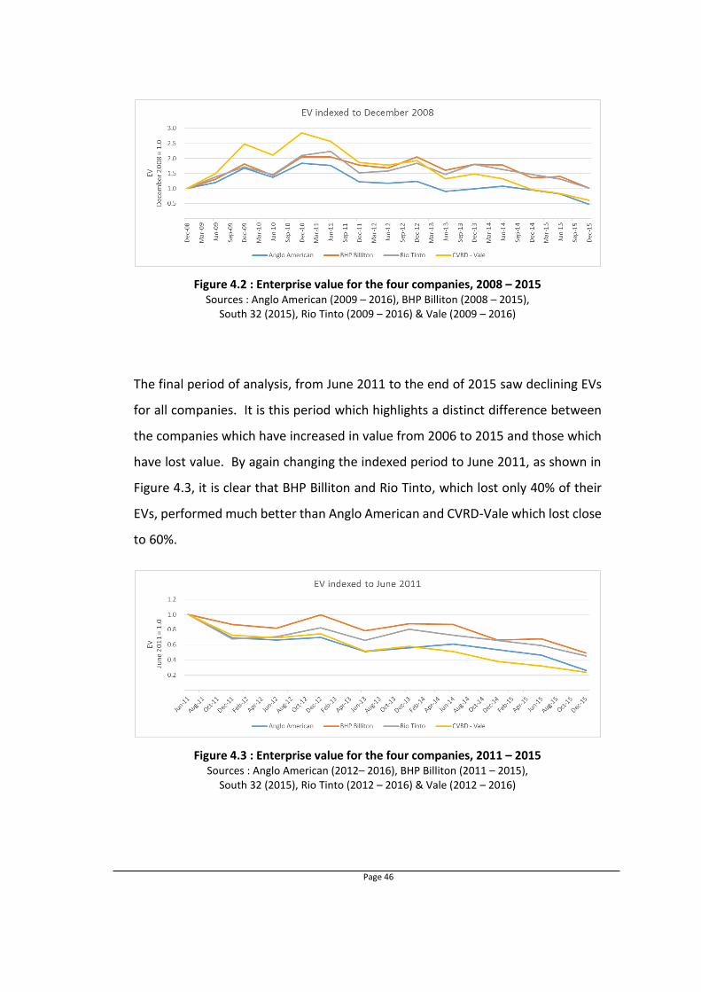
Page 46
Figure 4.2 : Enterprise value for the four companies, 2008 – 2015 Sources : Anglo American (2009 – 2016), BHP Billiton (2008 – 2015),
South 32 (2015), Rio Tinto (2009 – 2016) & Vale (2009 – 2016)
The final period of analysis, from June 2011 to the end of 2015 saw declining EVs
for all companies. It is this period which highlights a distinct difference between
the companies which have increased in value from 2006 to 2015 and those which
have lost value. By again changing the indexed period to June 2011, as shown in
Figure 4.3, it is clear that BHP Billiton and Rio Tinto, which lost only 40% of their
EVs, performed much better than Anglo American and CVRD-Vale which lost close
to 60%.
Figure 4.3 : Enterprise value for the four companies, 2011 – 2015 Sources : Anglo American (2012– 2016), BHP Billiton (2011 – 2015),
South 32 (2015), Rio Tinto (2012 – 2016) & Vale (2012 – 2016)

Page 47
Analysis of EV for the four companies over the 10 year period has shown the
following variable performance:
Rio Tinto significantly outperformed the other companies from 2007 to
2008;
Anglo American and CVRD-Vale underperformed from 2006 to 2008;
BHP Billiton was the least affected by the 2008 onset of the GFC;
CVRD-Vale had the best recovery of EV from 2008 to the end of 2010;
Anglo American had the worst recovery of EV from 2008 to the end of 2010
and then a similar poor performance to end of 2015; and
BHP Billiton and Rio Tinto significantly outperformed Anglo American and
CVRD-Vale from mid-2011 to the end of 2015.
Explanation of this difference in performance done in later sections of this study
should identify the key drivers for mining company value.
4.3 Production output
The production output for each company was plotted on a stacked area graph to
show the cumulative output from the different commodity segments per quarter
as shown in Figure 4.4 to Figure 4.7. The input data for these graphs is shown in
Appendix 7.9 to Appendix 7.12 respectively. Each commodity segment is indexed
back to Q4 2005, except for CVRD-Vale which only started producing from all
commodity segments in March 2010, and as such is indexed to Q1 2010.
4.3.1 Anglo American’s indexed production output
Figure 4.4 shows Anglo American’s indexed production output using input data
from Appendix 7.9. The company was producing from seven commodity segments
ceasing gold production at the end of 2007 with the sale of AngloGold Ashanti as
mentioned in Section 1.7.1.
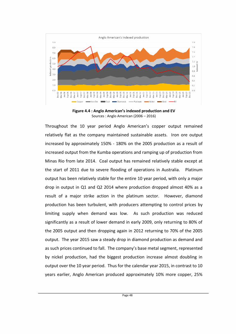
Page 48
Figure 4.4 : Anglo American’s indexed production and EV Sources : Anglo American (2006 – 2016)
Throughout the 10 year period Anglo American’s copper output remained
relatively flat as the company maintained sustainable assets. Iron ore output
increased by approximately 150% - 180% on the 2005 production as a result of
increased output from the Kumba operations and ramping up of production from
Minas Rio from late 2014. Coal output has remained relatively stable except at
the start of 2011 due to severe flooding of operations in Australia. Platinum
output has been relatively stable for the entire 10 year period, with only a major
drop in output in Q1 and Q2 2014 where production dropped almost 40% as a
result of a major strike action in the platinum sector. However, diamond
production has been turbulent, with producers attempting to control prices by
limiting supply when demand was low. As such production was reduced
significantly as a result of lower demand in early 2009, only returning to 80% of
the 2005 output and then dropping again in 2012 returning to 70% of the 2005
output. The year 2015 saw a steady drop in diamond production as demand and
as such prices continued to fall. The company’s base metal segment, represented
by nickel production, had the biggest production increase almost doubling in
output over the 10 year period. Thus for the calendar year 2015, in contrast to 10
years earlier, Anglo American produced approximately 10% more copper, 25%
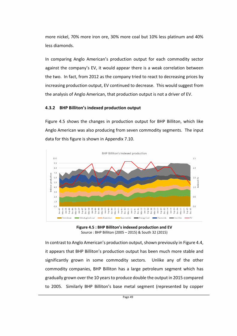
Page 49
more nickel, 70% more iron ore, 30% more coal but 10% less platinum and 40%
less diamonds.
In comparing Anglo American’s production output for each commodity sector
against the company’s EV, it would appear there is a weak correlation between
the two. In fact, from 2012 as the company tried to react to decreasing prices by
increasing production output, EV continued to decrease. This would suggest from
the analysis of Anglo American, that production output is not a driver of EV.
4.3.2 BHP Billiton’s indexed production output
Figure 4.5 shows the changes in production output for BHP Billiton, which like
Anglo American was also producing from seven commodity segments. The input
data for this figure is shown in Appendix 7.10.
Figure 4.5 : BHP Billiton’s indexed production and EV Source : BHP Billiton (2005 – 2015) & South 32 (2015)
In contrast to Anglo American’s production output, shown previously in Figure 4.4,
it appears that BHP Billiton’s production output has been much more stable and
significantly grown in some commodity sectors. Unlike any of the other
commodity companies, BHP Billiton has a large petroleum segment which has
gradually grown over the 10 years to produce double the output in 2015 compared
to 2005. Similarly BHP Billiton’s base metal segment (represented by copper

Page 50
output) and iron ore segments have also grown. Its base metal production was up
by 25% at the end of the 10 year period, with its iron ore segment producing
almost 250% of the 2005 output. Diamonds formed a small sector of BHP Billiton’s
business with declining production from mid-2010 to when the business was sold
at the end of 2012. It is only the energy coal and aluminium sectors which have
contracted slightly, down by around 20% by 2015 on the 2005 production. As with
the Anglo American comparison, there appears to be little correlation between
BHP Billiton’s EV and production output. Even as production has been increasing
from 2011 to 2015, EV continued to decline with declining prices. This again shows
that production output did not drive EV for the period under consideration.
4.3.3 Rio Tinto’s indexed production output
In comparison to BHP Billiton and Anglo American, Rio Tinto was only producing
from five different commodity sectors as of 2005, as shown in Figure 4.6. This
figure is based on input data from Appendix 7.11.
Figure 4.6 : Rio Tinto’s indexed production and EV Source : Rio Tinto (2006 – 2016a)
Rio Tinto’s copper output has remained relatively flat over the period, contracting
slightly for the last five years of the period. The company’s energy sector is
represented by thermal coal output from both the USA and Australia. In 2005
approximately 85% of Rio Tinto’s thermal coal output was from the USA. This
Page 51
dropped by 50% at the end of 2009 with a 50% initial public offering of its US
thermal coal operations which were operated by Cloud Peak Energy Inc (Rio Tinto,
2009). The following year, in 2010, the company fully divested from Cloud Peak
Energy Inc (Rio Tinto, 2010) resulting in Australia being the only source of its
thermal coal production. As such from Q1 2011 total thermal coal production for
the company was 15% of the 2005 output, with production remaining relatively
flat following this. Diamond production, like Anglo American’s output, is linked
closely to demand requirements thus reducing short term supply in line with
demand. Rio Tinto experienced a steady increase in iron ore production from early
2009 to doubling its 2005 output by the end of 2015.
The biggest change in production for the company was the increase in aluminium
production in 2007. This jump in aluminium output was as a result of Rio Tinto’s
acquisition of Alcan to become the world’s biggest aluminium producer. As a
result of this transaction its quarterly production output increased over four times
and has remained fairly stable for the remainder of the 10 years analysed. EV
jumped by almost 300% with the acquisition of Alcan and the increased aluminium
production. However, it would appear that as soon as prices dropped in 2008, EV
dropped as quickly, returning to close to the 2005 levels by the end of 2008. This
would suggest that whilst the rapid increase in production as a result of an
acquisition increased EV, declining commodity prices can have a similar negative
effect on EV. As such, commodity prices are analysed in a later section.
4.3.4 CVRD-Vale’s indexed production output
Figure 4.7 shows CVRD-Vale’s indexed production output and EV. The input data
used in this figure is shown in Appendix 7.12.

Page 52
Figure 4.7 : CVRD-Vale’s indexed production and EV Source : Vale (2006 – 2016)
At the end of 2005 CVRD-Vale was primarily an iron ore producer with some
copper assets. Following a strategic decision from 2006 to become a global
diversified miner, between 2006 and 2010 the company added coal, nickel,
fertilizer and bauxite segments to its business. Whilst production dropped in all
of these sectors following the GFC, after this it increased until another drop at the
end of 2010. Following this the company divested from bauxite however the other
segments continued to grow from 2011 to 2015. Throughout the 10 year period,
iron ore production remained relatively flat, with the diversification to other
commodities adding onto this stable iron ore base. In comparing the production
output and EV, it would appear that production output alone did not affect EV.
4.3.5 Correlation of production output to EV
The Pearson correlation coefficient of production output against EV is shown in
Table 4.1 obtained from data in Appendix 7.9 to Appendix 7.12. These values
confirm the inconsistent correlation that was observed in Figure 4.4 to Figure 4.7.
Table 4.1 : Pearson correlation coefficients of production output against EV
Anglo American BHP Billiton Rio Tinto CVRD-Vale
-0.4 0.2 0.6 -0.4
Medium (-) Low (+) High (+) Medium (-)

Page 53
As can be seen from the Pearson correlation coefficients for production output
against EV, there is weak correlation between production output and EV, except
for Rio Tinto’s anomaly associated with the acquisition of Alcan. This is because
analysis of production provides no link to the economic factors associated with the
extraction and sale of commodities. Increasing production in a commodity which
has declining prices and high extractive costs can destroy value and is not
represented in this metric. This lack of correlation can most clearly be seen in mid-
2008, when there was little change in production for all companies, yet the
company values dropped significantly for all companies. Rio Tinto was the only
company with a high correlation possibly as a result of the increase in aluminium
production as a result of the acquisition of Alcan which also resulted in a similar
increase in EV. The only other correlation which can be observed is that changes
to production appear to lag changes to EV. This would be expected as when a
company is doing well, and the EV increases, the reaction is to increase production.
Similarly when a company is not doing well, it reduces production in an attempt
to cut costs. As such, analysis purely of production was determined not to be a
driver of company value as it does not take into account the economic factors
associated with this production. However, the production output of each sector
was considered in the revenue calculation, as discussed in a later section of this
study. Commodity price was also analysed to find if price influences EV.
4.4 Commodity price
As discussed previously in detail in Section 2.3.1, commodity prices fluctuated
throughout the 10 year period. Appendix 7.13 to Appendix 7.15 show the indexed
commodity price for the major commodities over the 10 years analysed. These
graphs have been split into metal prices, bulk commodity prices and fertilizer
prices, with the three segments showing slightly different trends over the period.
From this it is clear that the commodities can be split into four main baskets, each
displaying similar trends. These baskets are gold, bulks and energy, metals and

Page 54
diamonds as shown in Figure 4.8. The bulks and energy basket was calculated by
taking the average of the iron ore, hard coking coal, thermal coal and crude oil
prices. The metals basket included copper, nickel, aluminium and platinum. The
fertilizer price which is represented by the phosphate rock price is not shown on
the graphs as it is not a key commodity and is a small contributor to CVRD-Vale’s
revenue. All prices were indexed back to the average price for the 2005 calendar
year.
Figure 4.8 : Indexed baskets of commodity prices Source : World Bank (2016)
From Figure 4.8 it is clear that the bulks and energy sector experienced the biggest
rise in pricing from 2006 to 2008 but, were similarly the hardest hit in 2008 due to
the GFC. This sector also suffered the biggest decline in price from 2010 to 2015.
The metals sector, which includes platinum, was similar to gold in doubling its
price from 2006 to 2008. However, when gold only dropped by around 20% with
the onset of the GFC, metal prices halved. The post GFC recovery of all the sectors
has been similar, however it is clear that those companies exposed to gold mining
have fared better than the others. Similarly those exposed to bulks and energy,
particularly iron ore and coal, should have had better earnings up until 2012
though they have been the hardest hit with declining prices from 2012 to 2015.

Page 55
Of the companies analysed, only Anglo American and BHP Billiton had some
exposure to gold. Anglo American sold out of the gold sector in 2007 and BHP
Billiton’s gold is an offtake product from its Olympic Dam operation. As such these
four companies were not able to capitalise on the rising gold price post the GFC.
Diamonds made a very small contribution to Anglo American’s and Rio Tinto’s
revenue streams so does not have a big influence on the two companies’ total
revenue. Thus for most companies their revenue stream is primarily dependent
on different exposure and production in the bulks and energy sector and metals
segment, with this to be discussed for each company in the next section.
4.5 Commodity price and production output mix
Revenue was analysed using a combination of production output and commodity
prices for each quarter. In essence this represents the changes in revenue
generated by the commodities portion of each of the companies. The results were
plotted on a stacked area graph, however instead of showing an indexed output
on the primary axis, a percentage contribution to revenue for each commodity
segment was used. The December 2005 data is the reported revenue contribution
for each of the segments for the FY2005, with changes to production and
commodity price varying the revenue for each segment. The graphs for the four
companies are shown in Figure 4.9 to Figure 4.12 drawn from data in Appendix
7.16 to Appendix 7.19. As a check of the accuracy of the calculations, for Anglo
American the actual reported revenue for 2015 was 70% of the 2005 level whilst
the calculated value was 63%. This difference is because the estimated revenue
uses a single commodity price and commodity production per segment, when in
reality a segment may be made up of a number of different commodities.
However, for the purpose of this comparison, the estimated revenue calculation
is a good representation of the total revenue contribution of each commodity.

Page 56
4.5.1 Anglo American’s revenue
Figure 4.9 shows Anglo American’s estimated revenue which was drawn using
input data in Appendix 7.16. This has been calculated by multiplying the indexed
commodity price by the indexed production output for each sector.
Figure 4.9 : Anglo American’s estimated revenue and EV Source : Anglo American (2006 – 2016)
As shown in Figure 4.9, in 2005 almost 50% of Anglo American’s revenue was made
up of non-mining based business. This included its steel businesses Scaw Metals
and Samancor group, the sugar producer Tongaat-Hulett and a paper and
packaging group Mondi. This lower reliance on mineral commodities from 2005
to 2008 when prices were booming could have been one of the reasons why Anglo
American underperformed compared to the other companies (as indicated in
Section 4.2) as it was not able to capitalise on booming commodity prices. The
revenue contribution of this “others” group declined from 2005 to contribute
around 10% of revenue as of 2015 as the company returned its focus on
commodities. This included the disposal of the Mondi group in 2007 as discussed
in Section 1.7.1.
The increased revenue from higher coal prices from 2005 to mid-2008 can be seen
as a big contributor to Anglo American’s revenue. An increase in coal and iron ore
production over the 10 year period, as shown previously in Figure 4.4, has been
Page 57
largely offset by declining prices in these sectors from mid-2011 to 2015. From
2010 to 2013 approximately 40% of its revenue was from iron ore and coal. This
sector has had the biggest decline in prices from 2010 to 2015 meaning that Anglo
American’s revenue has been dropping, resulting in declining EV over this period.
Unfortunately, as the company has started to increase iron ore output from late
2014 (as shown in Figure 4.4) with the commissioning of the Minas Rio project,
this has been offset by faster declining prices meaning revenue from the sector
continued to contract.
Revenue from copper, platinum and nickel has remained relatively flat between
2006 and 2015 except for a slight decline in 2008 during the GFC. However in total
these two sectors contributed less than 20% of revenue for most of the 10 year
period. Whilst Figure 4.4 shows nickel production growing from 2012 – 2015, it is
such a small contributor to revenue that this had little influence on the total
company’s EV.
In comparing the estimated revenue to the EV, there appears to be a very good
correlation between the two. The Pearson correlation, calculated between total
revenue and EV, is very high at 0.9 as discussed later in this report. Apart from a
slight drop in EV in late 2009/early 2010, which could be as a result of post GFC
sentiment, in general the EV tracks very closely to estimated revenue. This would
suggest that revenue is a key driver of EV for Anglo American, and could explain
some of the trends in terms of the company’s performance. For example, the
lower increase in EV from 2006 to 2008 compared to the companies was primarily
as a result of the company’s higher exposure to non-commodity businesses. Then
its slower recovery from 2008 to 2010 was due to the flat production in its iron
ore and coal business, when prices were booming within these sectors. Finally,
the faster decline from 2010 to 2015 is a consequence of its exposure to coal and
iron ore, both of which have been the worst price performers over this period.

Page 58
4.5.2 BHP Billiton’s revenue
BHP Billiton is one of the two companies which increased its EV by approximately
15% from 2006 to 2015. It was the best performer of the four companies during
the GFC commodity price crash, and together with Rio Tinto has significantly
outperformed the other two companies from mid-2011 to 2015 as shown in Figure
4.1. Its revenue mix is shown in Figure 4.10 drawn from data in Appendix 7.17.
Figure 4.10 : BHP Billiton’s estimated revenue and EV Source : BHP Billiton (2005 – 2015) & South 32 (2105)
As of the end of 2005 the company was fairly well diversified, with approximately
20% of its revenue each from petroleum, aluminium, base metals and iron ore.
These sectors grew primarily on higher commodity prices, though iron ore
production was up by 20% in mid-2008 compared to 2005 (Figure 4.5) meaning it
became a bigger contributor to revenue. It appears that BHP Billiton was the
company least affected by the GFC due to a steady output of iron ore and
petroleum which remained at above the 2005 output during the course of 2008.
Then following the GFC, the company started to increase iron ore and petroleum
production (Figure 4.5) with these two sectors growing to contribute over half of
the company’s revenue by 2011. It is likely that the strong recovery in EV from
2008 to 2011 can be attributed to this exposure and the increased production in
these sectors. Copper also slightly grew to contribute around 20% of BHP Billiton’s
revenue from 2013. The consistent revenue from aluminium and base metals,

Page 59
which have been less affected by declining prices from 2011, have resulted in a
lower decline in EV than Anglo American and Rio Tinto which have a bigger
exposure to iron ore.
In comparing BHP Billiton’s EV to total theoretical revenue, like Anglo American it
is clear that there is a close correlation between the two. As with Anglo American
there appears to be a drop in EV in late 2009, and a similar drop in late 2012, both
possibly as a result of pricing speculation. However, in general the trend appears
to be close as is confirmed by the Pearson correlation which is high at 0.8.
4.5.3 Rio Tinto’s revenue
Rio Tinto was by far the best performer from 2005 to 2008 as shown previously in
Figure 4.1. It would appear this success can primarily be attributed to the
company’s iron ore, copper and aluminium divisions as shown in Figure 4.11
drawn using data from Appendix 7.18.
Figure 4.11 : Rio Tinto’s estimated revenue and EV Source : Rio Tinto (2006 – 2016a)
Rising iron ore prices from 2005 to 2008 resulted in the iron ore segment revenue
increasing almost fourfold over the same period. Similarly, the acquisition of Alcan
in 2007 resulted in aluminium production increasing almost fivefold, and the
aluminium sector contributing close to one-third of revenue in mid-2008. Energy
revenue, comprising Rio Tinto’s thermal coal business, also grew in this period,
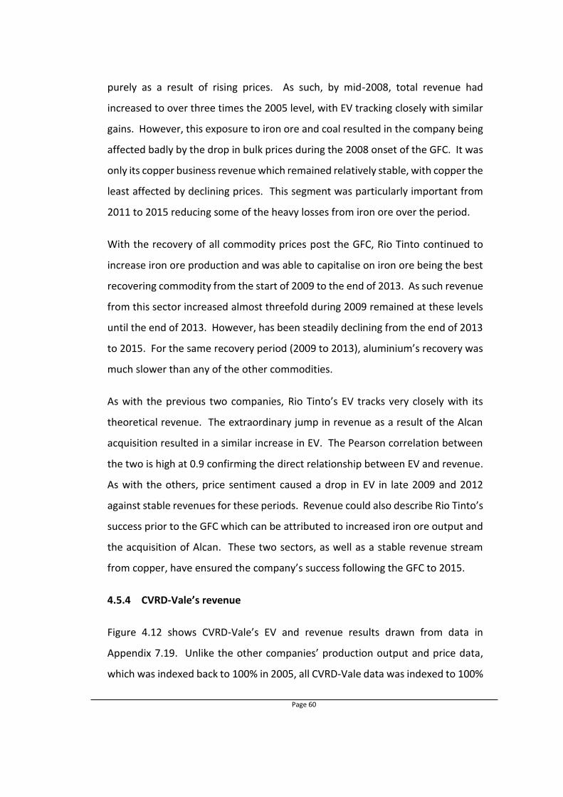
Page 60
purely as a result of rising prices. As such, by mid-2008, total revenue had
increased to over three times the 2005 level, with EV tracking closely with similar
gains. However, this exposure to iron ore and coal resulted in the company being
affected badly by the drop in bulk prices during the 2008 onset of the GFC. It was
only its copper business revenue which remained relatively stable, with copper the
least affected by declining prices. This segment was particularly important from
2011 to 2015 reducing some of the heavy losses from iron ore over the period.
With the recovery of all commodity prices post the GFC, Rio Tinto continued to
increase iron ore production and was able to capitalise on iron ore being the best
recovering commodity from the start of 2009 to the end of 2013. As such revenue
from this sector increased almost threefold during 2009 remained at these levels
until the end of 2013. However, has been steadily declining from the end of 2013
to 2015. For the same recovery period (2009 to 2013), aluminium’s recovery was
much slower than any of the other commodities.
As with the previous two companies, Rio Tinto’s EV tracks very closely with its
theoretical revenue. The extraordinary jump in revenue as a result of the Alcan
acquisition resulted in a similar increase in EV. The Pearson correlation between
the two is high at 0.9 confirming the direct relationship between EV and revenue.
As with the others, price sentiment caused a drop in EV in late 2009 and 2012
against stable revenues for these periods. Revenue could also describe Rio Tinto’s
success prior to the GFC which can be attributed to increased iron ore output and
the acquisition of Alcan. These two sectors, as well as a stable revenue stream
from copper, have ensured the company’s success following the GFC to 2015.
4.5.4 CVRD-Vale’s revenue
Figure 4.12 shows CVRD-Vale’s EV and revenue results drawn from data in
Appendix 7.19. Unlike the other companies’ production output and price data,
which was indexed back to 100% in 2005, all CVRD-Vale data was indexed to 100%

Page 61
in June 2010. This was because this was the first period where the company
produced from all commodity sectors. EV is also only shown from mid-2006 due
to a share split in early 2006.
Figure 4.12 : CVRD-Vale’s estimated revenue and EV Source : Vale (2006 – 2016)
CVRD-Vale’s primary commodity has traditionally been iron ore which contributed
almost three-quarters of its revenue in 2005. In addition to this, in 2005 a 10%
contribution was from its logistic business and aluminium and less than 5% from
base metals and copper. A jump in nickel production, along with price growth
from iron ore, resulted in revenue doubling from 2005 to mid-2008. However, it
appears price expectations around iron ore resulted in a drop in EV in mid-2007
prior to the onset of the GFC.
It was CVRD-Vale’s exposure to iron ore which caused total revenue, and as such
company value, to drop considerably in 2008, but similarly recovered to pre-GFC
levels in the following years. Increased production of coal, copper and fertilizer
from 2010, as shown in Figure 4.7, contributed the least to earnings, primarily due
to declining prices in these commodities over the same period. As such, where
iron ore ensured recovery in 2009, this same sector was the worst performer in
terms of price from 2013 to 2015 which meant that CVRD-Vale was the worst
performer in terms of EV over the same period.

Page 62
Thus the EV of CVRD-Vale can be predominately matched to the price cycles of
iron ore. As such revenue has tracked EV with a high correlation of 0.7. Other
than the unexplained drop in mid-2007, and the similar drops to the other
companies in late 2009, changes to EV appear to be as a result of changes to
revenue. Good growth in 2006 to 2008 was brought to an abrupt halt in 2008 by
the GFC, followed by better than average recovery of prices post-GFC which
ensured the rapid recovery of EV. Poor performance in this sector from 2013 to
2015 resulted in EV contracting to values below the 2006 level as of the end of
2015.
4.5.5 Correlation of revenue to EV
As discussed for each company in Section 4.5, the Pearson correlation coefficient
of revenue against EV is shown in Table 4.2 obtained from data in Appendix 7.16
to Appendix 7.19. These values are all above 0.5 suggesting that there is a very
strong correlation between revenue and EV.
Table 4.2 : Pearson correlation coefficients of revenue against EV
Anglo American BHP Billiton Rio Tinto CVRD-Vale
0.9 0.8 0.9 0.7
High (+) High (+) High (+) High (+)
In addition to the high correlation coefficient, graphically the correlation between
company value and revenue can be clearly seen in Figure 4.9 to Figure 4.12. The
total revenue tracks the EV for all the companies. As such, from both the Pearson
correlation coefficient and graphical analysis of the commodity price and
production mix compared to EV, it was determined that revenue is a strong driver
of company value. It was therefore classified as a key value driver of company
value. Since revenue is determined by both commodity price and production,
companies must ensure that they are increasing production on commodities with
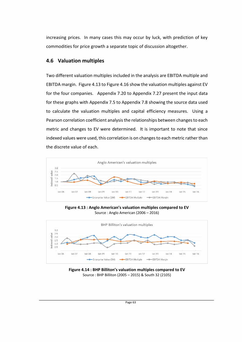
Page 63
increasing prices. In many cases this may occur by luck, with prediction of key
commodities for price growth a separate topic of discussion altogether.
4.6 Valuation multiples
Two different valuation multiples included in the analysis are EBITDA multiple and
EBITDA margin. Figure 4.13 to Figure 4.16 show the valuation multiples against EV
for the four companies. Appendix 7.20 to Appendix 7.27 present the input data
for these graphs with Appendix 7.5 to Appendix 7.8 showing the source data used
to calculate the valuation multiples and capital efficiency measures. Using a
Pearson correlation coefficient analysis the relationships between changes to each
metric and changes to EV were determined. It is important to note that since
indexed values were used, this correlation is on changes to each metric rather than
the discrete value of each.
Figure 4.13 : Anglo American’s valuation multiples compared to EV Source : Anglo American (2006 – 2016)
Figure 4.14 : BHP Billiton’s valuation multiples compared to EV Source : BHP Billiton (2005 – 2015) & South 32 (2105)

Page 64
Figure 4.15 : Rio Tinto’s valuation multiples compared to EV Source : Rio Tinto (2006 – 2016a)
Figure 4.16 : CVRD-Vale’s valuation multiples compared to EV Source : Vale (2006 – 2016)
As can be seen from Figure 4.13 to Figure 4.16 the EBITDA multiple tracks EV
relatively closely for all the companies except BHP Billiton, where the EBITDA
multiple has remained relatively flat. In contrast there is little correlation with
EBITDA margin, with little movement in this metric over the 10 years for all
companies. To confirm these observations the Pearson coefficient was calculated
to determine the correlation between the valuation multiples and EV.
4.6.1 Analysis of EBITDA multiple
Table 4.3 shows the Pearson correlation coefficient for EBITDA multiples for the
four companies. These are based on the data included in Figure 4.13 to Figure
4.16.
Table 4.3 : Pearson correlation coefficients of EBITDA multiple against EV
Anglo American BHP Billiton Rio Tinto CVRD-Vale
0.6 0.4 0.6 0.6
High (+) Medium (+) High (+) High (+)

Page 65
From these coefficient values, it can be seen that there is a high correlation
between changes to EBITDA multiple and EV for all companies except BHP Billiton,
which was slightly below 0.5. This is in line with the observations from the graphs
where EBITDA multiple tracks EV closely. An alternate analysis, as shown in Figure
4.17, was to compare the EBITDA multiples of each of the companies, rather than
the indexed values.
Figure 4.17 : EBITDA multiples for the four mining companies Sources : Anglo American (2006 – 2016), BHP Billiton (2005 – 2015),
South 32 (2015), Rio Tinto (2006 – 2016a) & Vale (2006 – 2016)
Other than CVRD-Vale being quite volatile during the GFC when earnings were also
unstable, on average all companies are within the window of around 6.0 EBITDA
multiple. The EBITDA multiple for BHP Billiton, the lowest for most of the period,
has remained relatively stable around 4 for the entire period. Anglo American and
Rio Tinto have tracked fairly closely throughout the period, indicating no major
difference between EV to earnings between the two. This would suggest that the
levels of EBITDA multiple are not a key value driver of company value.
In summary, based on the Pearson coefficient between EBITDA multiple and EV,
there is a high correlation. As such this suggests that EBITDA multiple is a key
driver of company value, however more so changes to EBITDA multiple rather than
the actual value of such.

Page 66
4.6.2 Analysis of EBITDA margin
Analysis of the previously shown Figure 4.13 to Figure 4.16 suggest that there is
little correlation between EBITDA margin and EV. The Pearson correlation
coefficients confirm this as shown in Table 4.4.
Table 4.4 : Pearson correlation coefficients of EBITDA margin against EV
Anglo American
BHP Billiton Rio Tinto CVRD-Vale
0.7 0.1 -0.1 0.1
High (+) Low (+) Low (-) Low (+)
EBITDA margin, a measure of the portion of revenue which is earnings compared
to costs, has a very low Pearson correlation coefficient against EV in all the
companies except Anglo American. The reason for this high correlation for Anglo
American could possibly related to the company’s efforts to decrease their EBITDA
margin from 2011 when at the same time EV was declining. For Rio Tinto, there is
a negative low correlation between EV and EBITDA margin. Because of this
variability, in terms of correlation to EV it appears that EBITDA margin is not a
value driver. Similarly in comparing the EBITDA margin between companies as
shown in Figure 4.18, there appears to be a weak correlation between the
companies which performed well, and those which did not do as well.
Figure 4.18 : EBITDA margins for the four mining companies Sources : Anglo American (2006 – 2016), BHP Billiton (2005 – 2015),
South 32 (2015), Rio Tinto (2006 – 2016a) & Vale (2006 – 2016)
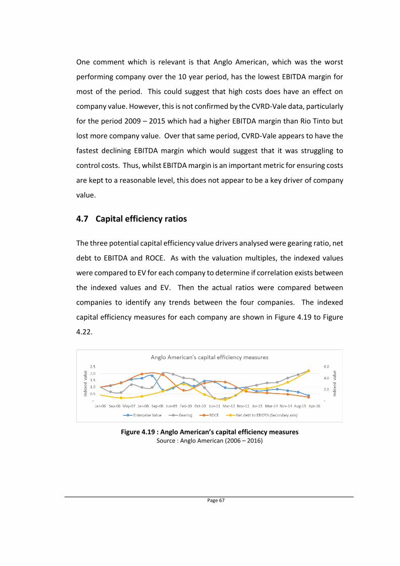
Page 67
One comment which is relevant is that Anglo American, which was the worst
performing company over the 10 year period, has the lowest EBITDA margin for
most of the period. This could suggest that high costs does have an effect on
company value. However, this is not confirmed by the CVRD-Vale data, particularly
for the period 2009 – 2015 which had a higher EBITDA margin than Rio Tinto but
lost more company value. Over that same period, CVRD-Vale appears to have the
fastest declining EBITDA margin which would suggest that it was struggling to
control costs. Thus, whilst EBITDA margin is an important metric for ensuring costs
are kept to a reasonable level, this does not appear to be a key driver of company
value.
4.7 Capital efficiency ratios
The three potential capital efficiency value drivers analysed were gearing ratio, net
debt to EBITDA and ROCE. As with the valuation multiples, the indexed values
were compared to EV for each company to determine if correlation exists between
the indexed values and EV. Then the actual ratios were compared between
companies to identify any trends between the four companies. The indexed
capital efficiency measures for each company are shown in Figure 4.19 to Figure
4.22.
Figure 4.19 : Anglo American’s capital efficiency measures Source : Anglo American (2006 – 2016)

Page 68
Figure 4.20 : BHP Billiton’s capital efficiency measures Source : BHP Billiton (2005 – 2015) & South 32 (2105)
Figure 4.21 : Rio Tinto’s capital efficiency measures Source : Rio Tinto (2006 – 2016a)
Figure 4.22 : CVRD-Vale’s capital efficiency measures Source : Vale (2006 – 2016)
As with the valuation multiples it is difficult to see any clear correlation between
the capital efficiency measures and EV for each of the companies. As such the
Pearson correlation coefficient was calculated for each capital efficiency measure.
4.7.1 Analysis of gearing ratio
Table 4.5 shows the Pearson correlation coefficients for gearing ratio against EV
for each of the companies. What is notable is that for two of the companies, Anglo
American and BHP Billiton the correlation coefficients are negative, and for the
other two the correlation coefficients are positive. This means that for those

Page 69
companies with a positive correlation, as gearing ratio increases EV also increases,
whereas when the correlation is negative the opposite occurs.
Table 4.5 : Pearson correlation coefficients of gearing ratio against EV
Anglo American BHP Billiton Rio Tinto CVRD-Vale
-0.5 -0.1 0.3 0.2
Medium (-) Low (-) Low (+) Low
Since the correlation is low for three of the companies this would suggest that
gearing ratio is not a driver of EV. Similarly, for Anglo American whilst the
correlation is medium, it is a negative correlation. This can be observed in Figure
4.19 that when the gearing ratio is high, EV is low and vice versa. However, this is
in contradiction to Rio Tinto which has a low/medium positive correlation with EV,
though this is much more difficult to observe in Figure 4.21. As an additional
comparison, Figure 4.23 shows a comparison of gearing ratios between the four
companies.
Figure 4.23 : Gearing ratios for the four mining companies Sources : Anglo American (2006 – 2016), BHP Billiton (2005 – 2015),
South 32 (2015), Rio Tinto (2006 – 2016a) & Vale (2006 – 2016)
In the first five years of Figure 4.23 there was a large spread between each of the
companies and only from 2011 where the ratios were more closely aligned. Rio
Tinto had an exceptionally high debt level from 2007 to 2009, primarily as a result
of the acquisition of Alcan. This acquisition boosted Rio Tinto’s aluminium
production and EV to make it the best performer among the four companies from
2006 to the GFC in mid-2008. What is surprising is that the high levels of debt

Page 70
associated with this acquisition did not appear to affect the company’s value
compared to the other companies. As such it would appear that in the boom and
recovery period from 2006 to 2010, gearing had little effect on EV. This is likely
because companies and investors were both chasing growth at any cost rather
than considering debt levels.
A trend is apparent from the period of declining prices from 2011. Whilst Anglo
American had the lowest gearing ratio as of 2011, it started to borrow with its net
debt rising from $USb1.4 at the end of 2011 to a peak of $USb13.5 in June 2015 as
shown in Appendix 7.5. This jump in debt was primarily associated with the
acquisition of the Minas Rio Iron Ore project. However, what is different to Rio
Tinto’s 2007 jump in debt is that little was added to EV with this increased debt.
CVRD-Vale was similar, with its gearing ratio increasing from 10% in June 2011 to
over 40% at the end of 2015. This is in comparison to BHP Billiton and Rio Tinto,
which both had better EV performances over this period and maintained their
gearing ratios at less than 25%.
Both BHP Billiton and Rio Tinto make mention of gearing in their 2015 annual
reports. BHP Billiton in its policy on debt and liquidity management indicated that
gearing should be a maximum of 40% (BHP Billiton, 2015). Rio Tinto was more
conservative suggesting that the gearing ratio should be kept between 20% and
30% in order to maintain a robust balance sheet (Rio Tinto, 2015). Neither Anglo
American nor CVRD-Vale made any mention on a focus or target for gearing, which
could explain why this ratio has been increasing for these companies.
Thus whilst analysis of EV and gearing ratio over the 10 year period suggests that
there is low a correlation, comparison of short periods indicate some correlation.
In the period of declining prices from mid-2011 to end of 2015, those companies
with faster increasing gearing ratios had more rapidly declining EV. In fact, when
the Pearson correlation coefficient between EV and gearing ratio is calculated over
the period from 2011 to 2015, the correlation was high and negative for all

Page 71
companies. This would suggest that gearing ratio is only a value driver in times of
declining commodity prices. In many cases this is when asset write downs are
common and as such investors and companies are concerned with levels of debt,
which as such can affect share price.
4.7.2 Analysis of net debt to EBITDA ratio
Net debt to EBITDA ratio is a similar measure to gearing ratio, in that it is a measure
of how much debt the company has. As such, as can be seen in Figure 4.19 to
Figure 4.22 the net debt to EBITDA and gearing ratios track relatively closely. Table
4.6 shows the Pearson correlation coefficients for net debt to EBITDA ratio against
EV.
Table 4.6 : Pearson correlation coefficients for net debt to EBITDA ratio against EV
Anglo American BHP Billiton Rio Tinto CVRD-Vale
-0.7 0.0 0.5 -0.4
High (-) Low Medium (+) Medium (-)
For all four companies there does not appear to be a consistent correlation
between net debt to EBITDA and EV. BHP Billiton had no correlation, meaning the
values are completely random to each other, whilst Anglo American and CVRD-
Vale had a negative correlation and Rio Tinto a positive one. This suggests that
based on the Pearson correlation coefficient analysis over the 10 year period, net
debt to EBITDA is not a driver of EV. Analysis of the values between companies,
as per Figure 4.24 confirm similar observations to those from gearing ratio
analysis.

Page 72
Figure 4.24 : Net debt to EBITDA ratio for the four mining companies Sources : Anglo American (2006 – 2016), BHP Billiton (2005 – 2015),
South 32 (2015), Rio Tinto (2006 – 2016a) & Vale (2006 – 2016)
As with the gearing ratio, the most noticeable trend is the sharply increasing net
debt to EBITDA ratio for Anglo American and CVRD-Vale from 2011 to 2015. Whilst
all companies have experienced an increase in net debt to EBITDA ratio as a result
of reduced earnings from the end of 2010, Anglo American has made the situation
worse by its rapid increase in debt. As with the gearing ratio, Rio Tinto’s debt
levels jumped with the acquisition of Alcan, however it succeeded in getting this
under control and to manageable levels over the next three years post the
acquisition. Both BHP Billiton and Rio Tinto have managed to maintain this ratio
between one and two from 2010 to 2015, giving the companies added flexibility
during times of decreasing earnings.
According to Price Waterhouse Coopers (2016) net debt to EBITDA ratios above
four should cause alarm, which none of these companies achieved. However, the
Price Waterhouse Coopers (2106) also indicated that the average net debt to
EBITDA ratio of the top 40 mining companies was 1.52 in 2014 and 2.46 in 2015.
Thus, the two companies, BHP Billiton and Rio Tinto, which have performed
relatively well over the 2010 – 2015 period, have net debt to EBITDA ratios less
than the average, and the other two companies which have performed poor have
ratios above this average.
To confirm the observation of correlation when prices were declining, the Pearson
correlation between net debt to EBITDA and EV for the period from end-2010 to

Page 73
end-2015 was calculated. All companies had a high negative correlation with
Anglo American, BHP Billiton and CVRD-Vale having a correlation coefficient of
-0.8 which suggests a very high correlation. This indicates that as with gearing
ratio, net debt to EBITDA ratio is particularly important in times of declining prices
and revenues. More specifically, in times of declining prices, the issue of net debt
must be kept to a manageable level depending on company size and industry
outlook, measured against value and company earnings.
4.7.3 Analysis of ROCE
The final capital efficiency metric, is ROCE which is a measure of how well a
company uses capital to generate returns. Analysing Figure 4.21 it appears that
for Rio Tinto, ROCE was relatively flat and thus had little influence on EV. However,
from the Pearson correlation coefficient, as shown in Table 4.7 Rio Tinto has a
medium negative correlation between ROCE and EV.
Table 4.7 : Pearson correlation coefficients of ROCE against EV
Anglo American BHP Billiton Rio Tinto CVRD-Vale
0.3 0.2 -0.5 0.5
Low (+) Low (+) Medium (-) Medium (+)
Both Rio Tinto and CVRD-Vale had a medium correlation, but one was negative
and the other positive. Both Anglo American and BHP Billiton had low positive
correlation coefficients. This range of values suggests that there is little
correlation between ROCE and EV. This is confirmed by analysing the ratios
between companies, as shown in Figure 4.25.

Page 74
Figure 4.25 : Return on capital employed for the four mining companies Sources : Anglo American (2006 – 2016), BHP Billiton (2005 – 2015),
South 32 (2015), Rio Tinto (2006 – 2016a) & Vale (2006 – 2016)
For all companies, the trend is generally downwards, as declining prices make it
more difficult to get the higher returns from the same capital. Anglo American is
particularly interesting to analyse since ROCE is the primary return measure used
by the company. In 2013, with the appointment of its new CEO Mark Cuttifani,
the company reported that it was focusing on ROCE, stating that “during the
downturn we have seen the mining industry’s ROCE plummet from around 24% to
about 10%” (Anglo American, 2014, p9). At that time its ROCE was around 11%
and the company committed to a target of a sustainable minimum ROCE of 15%
by 2016. The company was so committed to this that the CEO’s bonus was linked
to achieving this 15%. ROCE then decreased even further to 9% in 2014 and then
5% in 2015 (Anglo American, 2016b), suggesting that this measure was not being
achieved. None of the other companies reported their ROCE or made reference
to ROCE in their annual reports, suggesting that it is not an important metric for
them.
Whilst Anglo American is very focused on ROCE, the general spread and trends
shown in Figure 4.25 suggest that ROCE is not a key value driver of company value.
Where Anglo American had a significantly higher ROCE than Rio Tinto and CVRD-
Vale in 2008 and 2009, the company was the worst performer in terms of growing
company value. Similarly Rio Tinto had a number of years of very low ROCE yet it
has been one of the top performers of the four companies. As such it can be

Page 75
confirmed and concluded that based on this analysis and the Pearson correlation
coefficients, ROCE is not a key driver of company value.
4.8 Chapter summary
Analysis of the different metrics, using both a visual comparison of the relationship
between the metric and EV and by calculating the Pearson correlation coefficient
between each metric and EV, determined the key drivers of company value.
Analysis of production output on its own, not considering any of the economic
elements (especially price), indicated that there was no direct relationship
between production output and EV. Instead, this metric is only a value driver
when related with commodity price to derive revenue for the sector. Revenue
appeared to have the greatest influence on EV, and as such is the most important
key driver of EV and thus company value.
From analysis of the four companies it was found that there is a correlation
between EBITDA multiple and EV from both the observed trends between EV and
EBITDA multiple and the Pearson correlation coefficient for the four companies.
For the two debt based ratios, gearing and net debt to EBITDA, whilst both had
inconsistent correlations over the full 10 year period, they had high correlation to
EV for the period of declining prices from the end of 2010 to 2015. This would
suggest that both gearing and net debt to EBITDA ratios only influence company
value in times of declining commodity prices. EBITDA margin and ROCE were
found to have no correlation to EV, and as such are not key drivers of company
value.
Page 76
5 CONCLUSIONS AND RECOMMENDATIONS
5.1 Chapter overview
This final chapter provides an overview of the findings from the research study.
First, each of the potential value drivers analysed are reviewed and the key drivers
of company value identified. Then the observations of trends in company
performance are discussed and summarised. Finally, a number of
recommendations are provided for additional work given the outcomes of this
research study.
5.2 Findings
Eight different potential value drivers were analysed against EV to determine
which were key drivers of company value. These eight different potential drivers
are production output, commodity price, revenue (calculated based on the
production and commodity price), EBITDA multiple, EBITDA margin, gearing ratio,
net debt to EBITDA and ROCE. A number of findings were observed when
comparing each of these potential drivers with EV as discussed in the following
sub-sections.
5.2.1 Production output
Production output was found not to be a driver of company value. This is because
this metric does not take into account any economic factors, in particular
commodity price. For example, increasing production in a commodity which has
declining prices or high extractive costs can destroy rather than increase EV. This
was observed from 2011 to 2015, when whilst most of the four companies
increased total production output, EV decreased as a result of the declining
commodity prices. This suggests that production output alone is not a key driver
of company value.

Page 77
5.2.2 Commodity prices
Analysis of commodity price trends over the ten year period was found not to be
a driver of company value. This is because of the differing performance of the
different commodities’ prices over the period. Where diamonds prices have
remained relatively flat over the period, bulk commodities and energy prices
increased almost four fold from 2005 to mid-2008. As such any correlation
between company value and commodity prices must consider the exposure the
company has to each commodity. For non-diversified mining companies, which
only have exposure to a single commodity, the commodity price would be a key
value driver the price would directly influence revenue. However, for diversified
multi-commodity companies a more suitable metric is to combine production
output and commodity price to estimate revenue.
5.2.3 Revenue
Each company’s total revenue was analysed by combining production output and
commodity price for each quarter. This calculation represents an estimate of the
revenue for the different companies as a result of production output and price
variations. For all four companies this was found to have a very strong correlation
with EV from both the visual analysis of the results and by calculating the Pearson
correlation coefficient between the two. This suggests that the basket of
commodities which a company produces is a major driver of company value.
Companies must ensure that they are increasing production on commodities with
increasing prices. Unfortunately given the difficulties in accurate forecasting of
prices, and even if these are correct, the scarcity of mineral deposits and the long
lead time to develop a mining operation make it difficult for a company to pick and
choose the best performing commodities to invest in. However, some
consideration should be given to the selection of value adding mineral
commodities in order to drive revenue and consequently company value.

Page 78
5.2.4 EBITDA multiple
EBITDA multiple, which is a measure of company value as a multiple of annual
earnings, was found to have a high correlation to EV for all four companies. As
such, it is considered a key driver of company value. As EBITDA and revenue are
closely aligned, this would support the previous findings that revenue is a key
driver. As such, companies must focus on increasing earnings. Major decreases
to earnings will likely result in a similar drop in EV as the EBITDA multiple
normalises this out.
5.2.5 EBITDA margin
EBITDA margin is a measure of the relationship between revenue and earnings and
represents a company’s ability to keep its costs under control. Surprisingly EBITDA
margin was found not to have a correlation to EV for any of the companies except
Anglo American. As such it was not considered a key driver of company value.
Whilst there may not be a direct link Anglo American, which was the worst
performing company over the 10 year period, had the lowest EBITDA margin
indicating that cost control is an important consideration for company value.
5.2.6 Gearing ratio
The two metrics analysed which consider a company’s debt was gearing ratio and
net debt to EBITDA. Gearing ratio is a measure of debt to total company assets
and provides an indication of the company’s financial strength. A gearing ratio
that is too high increases financial risk. Gearing ratio was not found to have a
correlation with EV for the period from 2005 to 2011 when commodity prices were
rising, then crashed with the onset of the GFC and subsequently recovered.
However, from 2011 to 2015, a period which has seen commodity prices slowly
declining, there is a high correlation between EV and gearing. This would suggest
that gearing, and as such debt levels, are more important in times of declining
commodity prices and revenue. This is because during these periods, declining

Page 79
revenue raises concerns around a company’s ability to make debt repayments,
with these making up a growing portion of the company costs. During these times
companies must consider and manage their levels of debt.
5.2.7 Net debt to EBITDA ratio
Net debt to EBITDA ratio measures the company’s ability to pay back its debt from
earnings. As with gearing ratio, a noticeable trend was an increasing gearing ratio
and declining EV for Anglo American and CVRD-Vale from 2011 to 2015. However,
like gearing ratio, there was no correlation between net debt to EBIDTA ratio from
2005 to 2011. Only from 2011 to 2015 when prices were declining was there a
strong correlation between EV and net debt to EBITDA ratio. This confirms the
conclusions from gearing ratio which means that debt is a key driver of company
value in times of declining commodity prices.
5.2.8 ROCE
ROCE is a measure of a company’s use of capital to generate revenue. Interestingly
Anglo American consider this as an important metric that from 2014 they included
ROCE in its CEO’s performance measures. However, from analysis of the four
companies there was found to be no correlation between EV and ROCE. In fact
Rio Tinto had the lowest ROCE from end-2010 to 2015 yet was one of the better
performing companies during that period. Whilst Anglo American considers ROCE
to be an important metric, the data analysed in this study suggests otherwise. This
highlights the importance of understanding which metrics are key value drivers
and which have little correlation to company value.
5.2.9 Specific vale drivers over the 10 year period
The initial analysis of company value raised a number of key questions regarding
the differing performance of the four companies. Each of these were considered
in terms of the identified value drivers, to guide the determination of the metrics

Page 80
which most influence company value. Rio Tinto’s relative outperformance from
2005 – 2008 can be attributed to its acquisition of Alcan which increased the
company’s aluminium output almost fivefold and contributed to a doubling of
revenue. Whilst net debt increased significantly over this period, affecting gearing
ratio and net debt to EBITDA, this did not appear to have a negative effect on EV.
This is possibly due to the high commodity prices and increased revenue that was
generated during that period. As such this above par performance was primarily
revenue driven.
Anglo American’s underperformance in 2006 to 2008 is potentially due to its
reduced exposure to mineral commodities over that period. In 2005 over 50% of
its revenue was from non-mining business, much of which was not experiencing
the price growth that the commodity sector was. This meant that Anglo
American’s revenue growth was not the same as for the other mining companies,
and as such EV did not grow significantly. Similarly the company’s poor recovery
post-GFC can be attributed to a lack of capitalising on rising prices with flat iron
ore and coal production outputs. As such this is also linked to revenue.
BHP Billiton seems to have fared the best during the GFC price drop by increasing
iron ore and petroleum production output to minimise the effect on revenue. It
also appears that the company’s diversification strategy, ensuring a mix of
revenues rather than a focus on a single commodity has kept the volatility of
revenue to a minimum.
The poor performance of Anglo American and CVRD-Vale compared to BHP Billiton
and Rio Tinto from 2011 to 2015, when commodity prices were steadily declining,
appears to be as a result of rising debt within the two companies. This is reflected
in changes to the gearing ratio and net debt to EBITDA ratios which were rapidly
rising for both companies from 2011 to 2015. In contrast the better performing
companies, BHP Billiton and Rio Tinto, maintained stable gearing ratios and net
debt to EBITDA ratios during this same period.

Page 81
5.3 Research limitations
This research was limited to an analysis of four major international diversified
mining companies. As such the findings could be limited by the similar histories
and operating environments for the four companies. Similarly the full effect of
any mergers, demergers, acquisitions and sales were not able to be fully captured
in the analysis. These could have influenced EV in areas other than the analysed
metrics.
5.4 Recommendations for improved performance in mining
companies
Mining companies must ensure that they understand the importance of value
drivers when determining which metrics form part of their KPI’s. These drivers
must be those which management are able to influence and which have a high
impact on company value. From this study of value drivers, mining companies
should consider the following when selecting which metrics to focus on:
Revenue was found to be the number one value driver. Since revenue is
determined by both commodity price and production, companies must
ensure that they are increasing production of those commodities with
increasing prices;
Whilst companies that focused on single commodity’s experienced higher
revenues when specific commodities were booming, in times of lower
commodity prices revenue was similarly negatively affected. As such
diversified multi-commodity companies experienced much more stable
revenue, and thus EV, due to the variable performance of each
commodity. It is therefore recommended that, as much as practical,
major mining companies diversify across a range of commodities to
maintain more stable revenue and thus company value;

Page 82
Earnings was also found to be an important driver for company value and
as such companies must manage their EBITDA margin and EBITDA
multiples;
Debt related ratios appeared to only influence company value in times of
declining prices and as such declining revenue. Thus, during these
periods companies should consider and manage their debt levels in
relation to earnings and EV; and
ROCE was found to not have a high correlation with company value. Thus,
whilst Anglo American has selected ROCE as a KPI for senior management,
this study indicates that this metric does not have a high impact on EV. As
such the company should review this decision and confirm how changes to
ROCE impact company value.
5.5 Recommendations for future research work
On completion of the research study a number of additional queries arise leading
to possible future research and these are:
Whilst this study was focused on the period till the end of 2015, 2016 has
been an interesting year for mining companies. As of mid-November 2016,
all four companies’ share prices, and as such EVs have increased
significantly from the 2015 closing prices. BHP Billiton and Rio Tinto were
up by approximately 50%, CVRD-Vale well over doubled in price and Anglo
American was 390% higher. This would suggest that some changes in
market conditions and as such the identified key drivers for company value
should be confirmed for the 2016 period;
Other value drivers could be considered, particularly non-financial metrics.
This could include changes to company management; mergers, demergers,
acquisitions and sales; capital write-downs and other company
announcements; and

Page 83
The study could be expanded to include a broader range of mining
companies. This could include juniors and less diversified companies to
analyse if these same value drivers are relevant for the entire industry.

Page 84
6 REFERENCES
Anglo American (2006) Annual Report 2005. INTERNET http://www.angloamerican.com/~/media/Files/A/Anglo-American-PLC-V2/investors/a-reports/2006rep/ar2005a/ar2005a.pdf Cited 10 July 2016.
Anglo American (2007) Annual Report 2006. INTERNET http://www.angloamerican.com/~/media/Files/A/Anglo-American-PLC-V2/investors/a-reports/2007rep/annual_report_2006.pdf Cited 10 July 2016.
Anglo American (2008) Annual Report 2007. INTERNET http://ar07.angloamerican.solutions.investis.com/ Cited 10 July 2016.
Anglo American (2009) Annual Report 2008, INTERNET http://www.angloamerican.com/~/media/Files/A/Anglo-American-PLC-V2/investors/a-reports/2009rep/ar2008.pdf Cited 10 July 2016.
Anglo American (2010) Annual Report 2009. INTERNET http://www.angloamerican.com/~/media/Files/A/Anglo-American-PLC-V2/investors/a-reports/2010rep/Anglo_American_2009_Annual_Report.pdf Cited 10 July 2016.
Anglo American (2011) Annual Report 2010. INTERNET http://www.angloamerican.com/~/media/Files/A/Anglo-American-PLC-V2/investors/a-reports/2011rep/angloamerican-annual-report-2010.pdf Cited 10 July 2016.
Anglo American (2012) Annual Report 2011, INTERNET http://www.angloamerican.com/~/media/Files/A/Anglo-American-PLC-V2/investors/reports/aa-annual-report-2011.pdf Cited 10 July 2016.
Anglo American (2013) Annual Report 2012. INTERNET http://www.angloamerican.com/~/media/Files/A/Anglo-American-PLC-V2/investors/reports/annual-report2012.pdf Cited 10 July 2016.
Anglo American (2014) Annual Report 2013. INTERNET http://www.angloamerican.com/~/media/Files/A/Anglo-American-PLC-V2/investors/reports/annual-report2013.pdf Cited 10 July 2016.
Anglo American (2015) Annual Report 2014. INTERNET http://www.angloamerican.com/~/media/Files/A/Anglo-American-PLC-V2/report-builder-2014/annual-report/aa-ar14-interactive-final.pdf Cited 10 July 2016.

Page 85
Anglo American (2016a) History. INTERNET http://www.angloamerican.com/about-us/history Cited 10 September 2016.
Anglo American (2016b) Annual Report 2015. INTERNET http://www.angloamerican.com/~/media/Files/A/Anglo-American-PLC-V2/documents/aa-ar-15.pdf Cited 10 July 2016.
Baurens, S. (2010) Valuation of metals and mining companies. INTERNET http://ehrenworthsyme.com/casadeleon/Docs/ValuationofMining.pdf Cited 5 July 2016.
Baxter, R. (2009) The global economic crisis and its impact on South Africa and the country’s mining industry. South Africa: Chamber of Mines.
Beattie, A. (2016) A beginners guide to mining stocks. INTERNET http://www.investopedia.com/articles/basics/12/beginners-guide-mining-stocks.asp Cited 5 July 2016.
BHP Billiton (2005) Annual Report 2005. INTERNET http://www.bhpbilliton.com/~/media/bhp/documents/investors/reports/2005/bhpb_ltd_concise_ar05.pdf?la=en Cited 10 July 2016.
BHP Billiton (2006) Annual Report 2006. INTERNET http://www.bhpbilliton.com/~/media/bhp/documents/investors/reports/2006/bhpbreview2006.pdf?la=en Cited 10 July 2016.
BHP Billiton (2007) Annual Report 2007. INTERNET http://www.bhpbilliton.com/~/media/bhp/documents/investors/reports/2007/bhpbannualreview07.pdf?la=en Cited 10 July 2016.
BHP Billiton (2008) Annual Report 2008. INTERNET http://www.bhpbilliton.com/~/media/bhp/documents/investors/reports/2008/annualreport2008.pdf?la=en Cited 10 July 2016.
BHP Billiton (2009) Annual Report 2009. INTERNET http://www.bhpbilliton.com/~/media/bhp/documents/investors/reports/2009/annualreport2009.pdf?la=en Cited 10 July 2016.
BHP Billiton (2010) Annual Report 2010. INTERNET http://www.bhpbilliton.com/~/media/bhp/documents/investors/reports/2010/bhpbillitonannualreport2010.pdf?la=en Cited 10 July 2016.
BHP Billiton (2011) Annual Report 2011. INTERNET http://www.bhpbilliton.com/~/media/bhp/documents/investors/reports/2011/bhpbillitonannualreport2011.pdf?la=en Cited 10 July 2016.

Page 86
BHP Billiton (2012) Annual Report 2012. INTERNET http://www.bhpbilliton.com/~/media/bhp/documents/investors/reports/2012/bhpbillitonannualreport2012.pdf?la=en Cited 10 July 2016.
BHP Billiton (2013) Annual Report 2013. INTERNET http://www.bhpbilliton.com/~/media/bhp/documents/investors/reports/2013/bhpbillitonannualreport2013.pdf?la=en Cited 10 July 2016.
BHP Billiton (2014a) Creation of new global metals and mining company to accelerate portfolio simplification. INTERNET http://www.bhpbilliton.com/investors/news/creation-of-new-global-metals-and-mining-company Cited 14 September 2016.
BHP Billiton (2014b) Annual report 2014. INTERNET http://www.bhpbilliton.com/~/media/bhp/documents/investors/reports/2014/bhpbillitonannualreport2014_interactive.pdf?la=en Cited 10 July 2016.
BHP Billiton (2015) Annual report 2015. INTERNET http://www.bhpbilliton.com/~/media/bhp/documents/investors/annual-reports/2015/bhpbillitonannualreport2015.pdf?la=en Cited 10 July 2016.
BHP Billiton (2016a) Our history. INTERNET http://www.bhpbilliton.com/aboutus/ourcompany/ourhistory Cited 14 September 2016.
BHP Billiton (2016b) About us; Our strategy delivers. INTERNET http://www.bhpbilliton.com/aboutus/strategy Cited 14 September 2016.
Bhullar, P.S. & Bhatnagar, D. (2013) Theoretical framework : EV vs Stock price – A better measurement of firm value. International Journal of Commerce, Business and Management. Vol 2 No. 6. 335 – 343.
Biesheuvel, T. & Crowley K. (2015) Anglo overtakes Glencore as worst performing FTSE-100 stock. INTERNET http://www.bloomberg.com/news/articles/2015-12-09/anglo-draws-level-with-glencore-as-worst-stock-in-u-k-ftse-100 Cited 10 September 2016.
Brahmbhatt, M. & Canuto, O. (2010) Natural resources and development strategy after the crisis. Economic Premise No. 1. Washington DC: World Bank.
Damodaran, A. (2007) Return on Capital (ROC), Return on Invested Capital (ROIC) and Return on Equity (ROE): Measurement and Implications, New York: Stern School of Business.
Deloitte (2012) Linking strategy to value. Journal of business strategy, Vol 33 Issue 4, 49-57.

Page 87
Deloitte (2016a) Mineral asset valuations. INTERNET https://www2.deloitte.com/za/en/pages/energy-and-resources/articles/life-cycle-2-valutions.html Cited 28 November 2016.
Deloitte (2016b) Tracking the trends 2016 – The top 10 issues mining companies will face in the coming year. INTERNET https://www2.deloitte.com/content/dam/Deloitte/global/Documents/Energy-and-Resources/gx-er-tracking-the-trends-2016.pdf Cited 12 July 2016.
Diamond Search Engine (2016) Diamond Trends Price Index. INTERNET http://www.diamondse.info/diamonds-price-index.asp Cited 5 July 2016.
Ernst & Young (2015) Debt in the mining sector. EY Global Mining & Metals Network, London.
Ellis, T.R. (2016) Comparable mineral properties – do they exist for market value appraisals, Mining Engineering Vol 68 No 5, 67-72.
Fernàndez, P. (2007) Company valuation methods – the most common errors in valuations; IESE Business School – University of Navarra Working Paper no 449, Barcelona.
FTSE Russell (2016) FTSE gold mines index series. INTERNET http://www.ftse.com/products/indices/Gold Cited 8 July 2016.
FXtop (2016) Major historic exchange rates. INTERNET http://fxtop.com/en/historical-exchange-rates.php Cited 1 September 2016.
Investopedia (2016a) Business valuation. INTERNET http://www.investopedia.com/terms/b/business-valuation.asp Cited 3 October 2016.
Investopedia (2016b) Enterprise value (EV), INTERNET http://www.investopedia.com/terms/e/enterprisevalue.asp Cited 1 September 2016
Krinks, P., Nieponice, G., King, T., Scheibehenne, V. & Vogt, T. (2011) Value Creating in Mining – More than Commodity Prices: The 2010 Value Creators Report, Boston: Boston Consulting Group.
Koller, T., Goedhart, M., & Wessels, D. (2005) Valuation: Measuring and managing the value of companies, 4th Ed., New Jersey: John Wiley & Sons.
Laerd Statistics (2016) Pearson Product-Moment Correlation. INTERNET https://statistics.laerd.com/statistical-guides/pearson-correlation-coefficient-statistical-guide.php Cited 13 October 2016.
Page 88
L.E.K Consulting (nd) Identifying and managing key value drivers, Executive Insights. Vol. 1, Iss. 1.
Loughran, T. & Wellman, J.W. (2010) New evidence on the relation between the enterprise multiple and average stock returns. Journal of Financial and Quantitative Analysis, Vol 46 No. 6, 1629 – 1650.
Macabacus (2016) Valuation multiples, INTERNET http://macabacus.com/valuation/multiples Cited 4 October 2016.
Maverick, J.B. (2015) What main factors affect share prices in the metals and mining sector. INTERNET http://www.investopedia.com/ask/answers/022615/what-main-factors-affect-share-prices-metals-and-mining-sector.asp Cited viewed 5 July 2016.
Maxwell, P. (2006) Mineral economics – an introduction. Monograph 24 – Australian Mineral Economics, Sydney: Australian Institute of Mining and Metallurgy.
Media, T. (2012) Understanding commodity super-cycles, INTERNET http://www.troymedia.com/2012/05/15/understanding-commodity-super-cycles/ Cited 11 December 2016.
Minerals Council of Australia (2015) Iron Ore & global markets. INTERNET http://www.ironorefacts.com/the-facts/iron-ore-global-markets/ Cited 14 September 2016.
NACVA (National Association of Certified Valuators and Analyst) (2008) Business valuations: Fundamentals, techniques and theory, Salt Lake City: NACVA.
Njowa, G., Clay, A.N., & Musingwini, C. (2013) A perspective on global harmonisation of major national mineral asset valuation codes, Resources Policy Vol. 39, 1 – 14.
Oxford Dictionary (2016) Value INTERNET https://en.oxforddictionaries.com/definition/value Cited 25 October 2016.
Pattabiraman, S. (2013) Growth vs profitability, The importance of ROCE. CFO Connect. March 2013. India.
Pederson, J.P. (2005) International directory of company histories. Vol 67. London: St James Press.
Price Waterhouse Coopers (2006) Mines 2006 - Let the good times roll. INTERNET https://www.pwc.com/ua/en/press-room/assets/pwc_mine_2006.pdf Cited 13 July 2016.

Page 89
Price Waterhouse Coopers (2007) Mine 2007 – Riding the wave. INTERNET https://www.pwc.co.za/en/assets/pdf/pwc-mining-review-07.pdf Cited 13 July 2016.
Price Waterhouse Coopers (2009) Mines 2009 - When the going gets tough…. INTERNET http://www.infomine.com/library/publications/docs/PricewaterhouseCoopers2009.pdf Cited 13 July 2016.
Price Waterhouse Coopers (2010) Mines 2010 – Back to the boom. INTERNET http://www.pwc.co.za/en/assets/pdf/mine-2010-back-to-the-boom.pdf Cited 13 July 2016.
Price Waterhouse Cooper (2011) Mines 2011 – The game has changed. INTERNET http://www.pwc.com/ua/en/industry/metal_mining/mining/publications/mine-2011.html Cited 13 July 2016.
Price Waterhouse Cooper (2012) Mines 2012 – The growing disconnect. INTERNET https://www.pwc.kz/en/publications/mine/mine-2012-eng.pdf Cited 13 July 2016.
Price Waterhouse Coopers (2013) Mine 2013 A confidence crisis. INTERNET https://www.pwc.com/gx/en/mining/publications/assets/pwc-mine-a-confidence-crisis.pdf Cited 13 July 2016.
Price Waterhouse Coopers (2015) Sustainable cost reduction in the mining sector. INTERNET https://www.pwc.com/ca/en/mining/publications/cost-reduction-mining-sector-2010-11-30-en.pdf Cited 13 July 2016.
Price Waterhouse Coopers (2016) Mines 2016 – Slower, lower, weaker .. but not defeated. INTERNET https://www.pwc.co.za/en/assets/pdf/mine-2016.pdf Cited 13 July 2016.
Rio Tinto (2006) Annual Report 2005. INTERNET http://www.portalchemy.com/Report.asp?ShareCode=RIO.L&arYear=2005 Cited 15 July 2016.
Rio Tinto (2007) Annual Report 2006. INTERNET https://bib.kuleuven.be/files/ebib/jaarverslagen/RioTinto_2006.pdf Cited 15 July 2016.
Rio Tinto (2008) Annual Report 2007. INTERNET http://www.riotinto.com/annualreport2007/services/downloads/index.html Cited 15 July 2016.

Page 90
Rio Tinto (2009) Annual Report 2008. INTERNET http://www.riotinto.com/documents/AnnualReport2008.pdf Cited 15 July 2016.
Rio Tinto (2010) Annual Report 2009. INTERNET http://www.riotinto.com/documents/rio_tinto_full_annualreport2009.pdf Cited 15 July 2016.
Rio Tinto (2011) Annual Report 2010. INTERNET http://www.riotinto.com/documents/riotinto_2010_ara.pdf Cited 15 July 2016.
Rio Tinto (2012) Annual Report 2011. INTERNET http://www.riotinto.com/documents/Investors/Rio_Tinto_2011_Annual_report.pdf Cited 15 July 2016.
Rio Tinto (2013) Annual Report 2012. INTERNET http://www.riotinto.com/documents/rio_tinto_2012_annual_report.pdf Cited 15 July 2016.
Rio Tinto (2014) Annual Report 2013. INTERNET http://www.riotinto.com/documents/RT_Annual_report_2013.pdf Cited 15 July 2016.
Rio Tinto (2015) Annual Report 2014. INTERNET http://www.riotinto.com/documents/RT_Annual_report_2014.pdf Cited 15 July 2016.
Rio Tinto (2016a) Annual Report 2015. INTERNET http://www.riotinto.com/documents/RT_Annual_Report_2015.pdf Cited 15 July 2016.
Rio Tinto (2016b) History. INTERNET http://www.riotinto.com/aboutus/history-4705.aspx Cited 16 September 2016.
Roberts, C. (2006) The valuation of advanced mining projects and operating mines: market comparable approaches. INTERNET www.infomine.com/library/publications/docs/roberts2006.pdf Cited 15 July 2016.
South African Mineral Asset Valuation Committee (SAMVAL), (2016), The South African code for reporting of mineral asset valuation. INTERNET http://www.samcode.co.za/samcode-ssc/samval Cited 9th June 2017.
Seccombe, A. (2015) Minas Rio aims to cut output costs, Business Day INTERNET http://www.bdlive.co.za/business/mining/2015/05/13/minas-rio-aims-to-cut-output-costs Cited 1 September 2016.

Page 91
Solly, I. (2013) Glencore Xstrata – The birth of a mining monster, London Mining Network Briefing paper – October 2013, INTERNET www.londonminingnetwork.org/wp-content/.../Glencore-Xstrata-merger-final-1310041.doc Cited 5 September 2016.
South 32 (2015) Annual Report 2015. INTERNET https://www.south32.net/CMSPages/GetFile.aspx?guid=a9c4ef48-785c-4ebb-9150-e7e96cb1005a Cited 20 July 2016.
Spector, J.B. (2012) Anglo American: A giant corporation between a big rock and a very hard place, Daily Maverick. INTERNET http://www.dailymaverick.co.za/article/2012-10-29-anglo-american-a-giant-corporation-between-a-big-rock-and-a-very-hard-place/#.V9gH3_l97IU Cited 13 September 2016.
Steiger, F. (2008) The validity of company valuation using discounted cash flow methods. European Business School.
The Steel index (2016) Coking coal index. INTERNET https://www.thesteelindex.com/en/cokingcoalindex/ Cited 10 October 2016.
Vale (2006) Annual Report Form 20-F 2005. INTERNET http://www.vale.com/EN/investors/information-market/annual-reports/20f/20FDocs/20F_2005_i.pdf Cited 12 July 2016.
Vale (2007) Annual Report Form 20-F 2006. INTERNET http://www.vale.com/EN/investors/information-market/annual-reports/20f/20FDocs/20F_2006_i.pdf Cited 12 July 2016.
Vale (2008) Annual Report Form 20-F 2007. INTERNET http://www.vale.com/EN/investors/information-market/annual-reports/20f/20FDocs/20F_2007_i.pdf Cited 12 July 2016.
Vale (2009) Annual Report Form 20-F 2008. INTERNET http://www.vale.com/EN/investors/information-market/annual-reports/20f/20FDocs/20F_2008_i.pdf Cited 12 July 2016.
Vale (2010) Annual Report Form 20-F 2009. INTERNET http://www.vale.com/EN/investors/information-market/annual-reports/20f/20FDocs/20F_2009_i.pdf Cited 12 July 2016.
Vale (2011) Annual Report Form 20-F 2010. INTERNET http://www.vale.com/EN/investors/information-market/annual-reports/20f/20FDocs/20F_2010_i.pdf Cited 12 July 2016.
Vale (2012a) Vale – Our history. Sao Paulo: Vale Brazil.

Page 92
Vale (2012b) Annual Report Form 20-F 2011. INTERNET http://www.vale.com/EN/investors/information-market/annual-reports/20f/20FDocs/20F_2011_i.pdf Cited 12 July 2016.
Vale (2013) Annual Report Form 20-F 2012. INTERNET http://www.vale.com/EN/investors/information-market/annual-reports/20f/20FDocs/20F_2012_i.pdf Cited 12 July 2016.
Vale (2014) Annual Report Form 20-F 2013. INTERNET http://www.vale.com/EN/investors/information-market/annual-reports/20f/20FDocs/20F_2013_i.pdf Cited 12 July 2016.
Vale (2015) Annual Report Form 20-F 2014. INTERNET http://www.vale.com/EN/investors/information-market/annual-reports/20f/20FDocs/Vale%2020-F%202014_i_novo.pdf Cited 12 July 2016.
Vale (2016) Annual Report Form 20-F 2015. INTERNET http://www.vale.com/EN/investors/information-market/annual-reports/20f/20FDocs/Vale%2020-F%202015_i.PDF Cited 12 July 2016.
Wilson, J. (2016) Anglo American eases executive bonus target, Financial Times. INTERNET https://www.ft.com/content/872490d2-dca5-11e5-827d-4dfbe0213e07 Cited 20 September 2016.
World Bank (2016) Commodity prices “Pink sheet”. INTERNET http://www.worldbank.org/en/research/commodity-markets#1 Cited 1 September 2016.
Yahoo Finance (2016a) Anglo American plc LSE historic share price. INTERNET https://uk.finance.yahoo.com/q/hp?s=AAL.L Cited 1 September 2016.
Yahoo Finance (2016b) BHP Billiton ASX historic share price. INTERNET https://uk.finance.yahoo.com/q/hp?s=BHP.AX Cited 1 September 2016.
Yahoo Finance (2016c) Rio Tinto LSE historic share price. INTERNET https://uk.finance.yahoo.com/q/hp?s=RIO.L Cited 1 September 2016.
Yahoo Finance (2016d) Rio Tinto LSE historic share price. INTERNET https://uk.finance.yahoo.com/q/hp?s=VALE Cited 1 September 2016.

Page 93
7 APPENDICES
Appendix 7.1 : Company sector summary - Anglo American Source : Anglo American (2006 – 2016)
Company Commodity grouping Sector summary Commodity for production analysis
Commodity price for revenue analysis
Anglo American
Platinum group metals
Mining of platinum, palladium, rhodium and by-product of copper, nickel and gold
Refined platinum production in ounces
Platinum price ($/oz)
Gold Mining of gold Gold production in ounces Gold price ($/oz)
Diamonds Mining of diamonds Diamond production in carats Diamond index price ($/ct)
Coal Includes both metallurgical and thermal coal
Total coal output including Australian metallurgical coal, Australian thermal coal, South African export thermal coal and South African domestic coal pricing
50% thermal coal & 50% coking coal (derived from the years that the company did report revenue split for thermal & coking coal, where the contribution was close to 50% from each)
Copper Copper output in tonnes Copper output in tonnes Copper price ($/mt)
Nickel, niobium & mineral sands
Mining of nickel, niobium and phosphates niobium
This will be represented by nickel output in ‘000 tonnes
Nickel price ($/mt)
Iron ore & manganese
Mining of iron ore and manganese
Total iron ore production including lump and fines in million tonnes
Iron ore cfr ($/dmtu)
Other mining, industrial & corporate
Includes zinc, Scaw metals, Highveld steel, Samancor (manganese), Tongaat-Hulett (sugar & aluminium)
No production analysis to occur for this
N/A

Page 94
Appendix 7.2 : Company sector summary - BHP Billiton Source : BHP Billiton (2005 – 2016) & South 32 (2015)
Company Commodity grouping Sector summary Commodity for production analysis
Commodity price for revenue analysis
BHP Billiton
Petroleum & potash
Exploration, development and production of oil and gas & potash
Total petroleum output which includes crude oil, condensate and natural gas liquids and natural gas in million barrels of oil equivalent (boe). Since potash is a minor contributor it is not included in the production analysis
Crude oil average ($/bbl)
Aluminium, manganese & nickel
Mining of bauxite, refining of bauxite into alumina and smelting of alumina into aluminium metal. Mining of manganese ore and production of manganese metal and alloys. Mining & production of nickel products
Aluminium is the main output and contributor to revenue for this sector the total aluminium output in ‘000 tonnes will be used for the production analysis
Aluminium ($/mt)
Base metals Mining of copper, silver, lead, zinc, molybdenum, uranium and gold.
Copper is the main contributor to revenue for this sector. Measured in ‘000 tonnes
Copper ($/mt)
Diamond and speciality productions
Mining of diamonds and titanium minerals
Diamond carats produced Diamond index price ($/ct)
Iron ore Mining of iron ore Iron ore in ‘000 tonnes Iron ore cfr ($/dmtu)
Metallurgical coal Mining of metallurgical coal Metallurgical coal in ‘000 tonnes Australian HCC coal FOB ($/t)
Energy coal Mining of thermal (energy) coal Energy (thermal) coal in ‘000
tonnes Australian thermal coal FOB ($/t)

Page 95
Appendix 7.3 : Company sector summary - Rio Tinto Source : Rio Tinto (2006 – 2016a)
Company Commodity grouping Sector summary Commodity for production analysis
Commodity price for revenue analysis
Rio Tinto
Aluminium
Mining of bauxite, refining of bauxite into alumina and smelting of alumina into aluminium metal.
Aluminium is the main output and contributor to revenue for this sector the total aluminium output in ‘000 tonnes will be used for the production analysis.
Aluminium ($/mt)
Iron ore Mining of iron ore Iron ore in ‘000 tonnes Iron ore cfr ($/dmtu)
Diamonds & industrial minerals
Mining of diamonds, Rio Tinto Iron and Titanium division (RTIT) which produces titanium dioxide, Rio Tinto Minerals & Dampier salt
As over 50% of this sectors revenue is from titanium dioxide since titanium dioxide price history is difficult to obtain, diamonds will be used
Diamonds ($/ct)
Copper Mining of copper Copper in ‘000 tonnes Copper ($/mt)
Energy Mining of thermal coal and uranium.
Majority of revenue from thermal coal thus total thermal coal output used.
Australian thermal coal FOB ($/t)
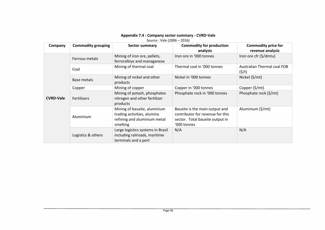
Page 96
Appendix 7.4 : Company sector summary - CVRD-Vale Source : Vale (2006 – 2016)
Company Commodity grouping Sector summary Commodity for production analysis
Commodity price for revenue analysis
CVRD-Vale
Ferrous metals Mining of iron ore, pellets, ferroralloys and managanese
Iron ore in ‘000 tonnes Iron ore cfr ($/dmtu)
Coal Mining of thermal coal Thermal coal in ‘000 tonnes Australian Thermal coal FOB
($/t)
Base metals Mining of nickel and other products
Nickel in ‘000 tonnes Nickel ($/mt)
Copper Mining of copper Copper in ‘000 tonnes Copper ($/mt)
Fertilizers Mining of potash, phosphates nitrogen and other fertilizer products
Phosphate rock in ‘000 tonnes Phosphate rock ($/mt)
Aluminium
Mining of bauxite, aluminium trading activities, alumina refining and aluminium metal smelting
Bauxite is the main output and contributor for revenue for this sector. Total bauxite output in ‘000 tonnes
Aluminium ($/mt)
Logistics & others Large logistics systems in Brazil including railroads, maritime terminals and a port
N/A N/A
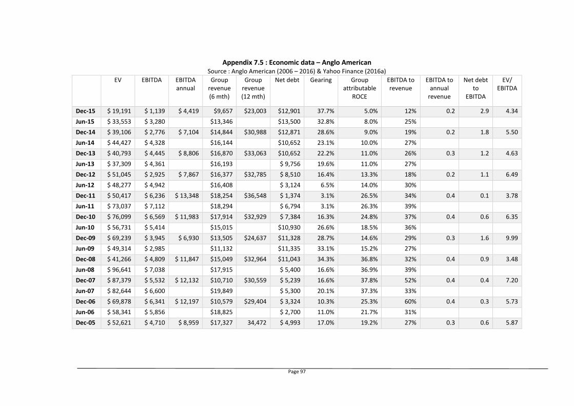
Page 97
Appendix 7.5 : Economic data – Anglo American Source : Anglo American (2006 – 2016) & Yahoo Finance (2016a)
EV EBITDA EBITDA annual
Group revenue (6 mth)
Group revenue (12 mth)
Net debt Gearing Group attributable
ROCE
EBITDA to revenue
EBITDA to annual
revenue
Net debt to
EBITDA
EV/ EBITDA
Dec-15 $ 19,191 $ 1,139 $ 4,419 $9,657 $23,003 $12,901 37.7% 5.0% 12% 0.2 2.9 4.34
Jun-15 $ 33,553 $ 3,280 $13,346 $13,500 32.8% 8.0% 25%
Dec-14 $ 39,106 $ 2,776 $ 7,104 $14,844 $30,988 $12,871 28.6% 9.0% 19% 0.2 1.8 5.50
Jun-14 $ 44,427 $ 4,328 $16,144 $10,652 23.1% 10.0% 27%
Dec-13 $ 40,793 $ 4,445 $ 8,806 $16,870 $33,063 $10,652 22.2% 11.0% 26% 0.3 1.2 4.63
Jun-13 $ 37,309 $ 4,361 $16,193 $ 9,756 19.6% 11.0% 27%
Dec-12 $ 51,045 $ 2,925 $ 7,867 $16,377 $32,785 $ 8,510 16.4% 13.3% 18% 0.2 1.1 6.49
Jun-12 $ 48,277 $ 4,942 $16,408 $ 3,124 6.5% 14.0% 30%
Dec-11 $ 50,417 $ 6,236 $ 13,348 $18,254 $36,548 $ 1,374 3.1% 26.5% 34% 0.4 0.1 3.78
Jun-11 $ 73,037 $ 7,112 $18,294 $ 6,794 3.1% 26.3% 39%
Dec-10 $ 76,099 $ 6,569 $ 11,983 $17,914 $32,929 $ 7,384 16.3% 24.8% 37% 0.4 0.6 6.35
Jun-10 $ 56,731 $ 5,414 $15,015 $10,930 26.6% 18.5% 36%
Dec-09 $ 69,239 $ 3,945 $ 6,930 $13,505 $24,637 $11,328 28.7% 14.6% 29% 0.3 1.6 9.99
Jun-09 $ 49,314 $ 2,985 $11,132 $11,335 33.1% 15.2% 27%
Dec-08 $ 41,266 $ 4,809 $ 11,847 $15,049 $32,964 $11,043 34.3% 36.8% 32% 0.4 0.9 3.48
Jun-08 $ 96,641 $ 7,038 $17,915 $ 5,400 16.6% 36.9% 39%
Dec-07 $ 87,379 $ 5,532 $ 12,132 $10,710 $30,559 $ 5,239 16.6% 37.8% 52% 0.4 0.4 7.20
Jun-07 $ 82,644 $ 6,600 $19,849 $ 5,300 20.1% 37.3% 33%
Dec-06 $ 69,878 $ 6,341 $ 12,197 $10,579 $29,404 $ 3,324 10.3% 25.3% 60% 0.4 0.3 5.73
Jun-06 $ 58,341 $ 5,856 $18,825 $ 2,700 11.0% 21.7% 31%
Dec-05 $ 52,621 $ 4,710 $ 8,959 $17,327 34,472 $ 4,993 17.0% 19.2% 27% 0.3 0.6 5.87

Page 98
Appendix 7.6 : Economic data – BHP Billiton Source : BHP Billiton (2005 – 2015), South 32 (2015) & & Yahoo Finance (2016b)
EV EBITDA EBITDA annual
Group revenue (6 mth)
Group revenue (12 mth)
Net debt Gearing Group attributable
ROCE
EBITDA to revenue
EBITDA to annual
revenue
Net debt to
EBITDA
EV/ EBITDA
Dec-15 $72,120 $5,994 $19,801 $26,016 25.3% 30%
Jun-15 $99,601 $15,101 $29,595 $22,479 $52,379 $24,819 24.0% 4.9% 67% 57% 0.8 3.37
Dec-14 $96,939 $14,494 $29,900 $24,900 22.4% 48%
Jun-14 $127,375 $13,774 $30,292 $33,258 $67,206 $25,786 23.2% 15.8% 41% 45% 0.9 4.20
Dec-13 $128,868 $16,518 $33,948 $27,100 32.9% 49%
Jun-13 $115,163 $14,865 $28,109 $33,764 $65,968 $29,105 28.8% 23.0% 44% 43% 1.0 4.10
Dec-12 $146,140 $13,244 $32,204 $30,400 31.0% 41%
Jun-12 $120,154 $12,811 $31,554 $19,140 $56,620 $23,607 26.0% 13.5% 67% 56% 0.7 3.81
Dec-11 $127,123 $18,743 $37,480 $21,500 25.0% 50%
Jun-11 $146,803 $15,600 $32,904 $22,922 $57,088 $5,823 9.2% 42.8% 68% 58% 0.2 4.46
Dec-10 $146,691 $17,304 $34,166 $7,915 6.0% 51%
Jun-10 $102,652 $13,675 $24,513 $28,222 $52,798 $3,308 6.3% 26.4% 48% 46% 0.1 4.19
Dec-09 $129,581 $10,838 $24,576 $7,915 15.1% 44%
Jun-09 $93,592 $4,275 $18,214 $20,431 $50,211 $5,586 12.1% 24.6% 21% 36% 0.3 5.14
Dec-08 $71,534 $13,939 $29,780 $4,168 9.5% 47%
Jun-08 $139,934 $16,864 $28,031 $33,934 $59,473 $8,458 17.8% 37.5% 50% 47% 0.3 4.99
Dec-07 $122,762 $11,167 $25,539 $12,200 28.0% 44%
Jun-07 $103,204 $10,633 $21,127 $25,359 $47,473 $9,971 25.0% 38.4% 42% 45% 0.5 4.88
Dec-06 $69,757 $10,494 $22,114 $7,200 20.3% 47%
Jun-06 $75,819 $17,098 $25,069 $21,019 $39,099 $8,200 27.2% 36.6% 81% 64% 0.3 3.02
Dec-05 $62,767 $7,971 18,080 $8,700 25.2% 44%
NB: 2015 data includes reported data from South 32 Annual reports

Page 99
Appendix 7.7 : Economic data – Rio Tinto Source : Rio Tinto (2006 – 2016a) & Yahoo Finance (2016c)
EV EBITDA EBITDA annual
Group revenue (6 mth)
Group revenue (12 mth)
Net debt Gearing Group attributable
ROCE
EBITDA to
revenue
EBITDA to annual
revenue
Net debt to
EBITDA
EV/ EBITDA
Dec-15 $67,902 $4,755 $12,058 $17,551 $36,785 $13,783 23.8% 4.9% 27% 33% 1.1 5.63
Jun-15 $88,536 $7,303 $19,234 $13,683 21.3% 38%
Dec-14 $99,239 $8,387 $18,840 $24,476 $50,041 $12,495 18.6% 13.1% 34% 38% 0.7 5.27
Jun-14 $109,628 $10,453 $25,565 $12,495 18.6% 41%
Dec-13 $121,222 $10,799 $20,953 $28,009 $54,599 $18,055 25.2% 8.3% 39% 38% 0.9 5.79
Jun-13 $98,878 $10,154 $26,590 $22,105 28.3% 38%
Dec-12 $124,023 $9,484 $20,095 $27,774 $55,566 $19,192 24.9% -1.8% 34% 36% 1.0 6.17
Jun-12 $106,153 $10,611 $27,792 $19,192 22.7% 38%
Dec-11 $102,094 $14,221 $28,521 $36,298 $65,354 $8,451 12.5% 13.4% 39% 44% 0.3 3.58
Jun-11 $150,505 $14,300 $29,056 $8,589 11.0% 49%
Dec-10 $141,382 $14,722 $25,978 $28,403 $55,171 $4,071 5.9% 20.7% 52% 47% 0.2 5.44
Jun-10 $97,887 $11,256 $26,768 $11,967 20.0% 42%
Dec-09 $115,906 $8,223 $14,312 $24,513 $44,036 $18,861 29.1% 9.5% 34% 33% 1.3 8.10
Jun-09 $93,168 $6,089 $19,523 $39,057 67.3% 31%
Dec-08 $67,381 $12,462 $23,870 $28,060 $58,065 $38,672 63.3% 16.1% 44% 41% 1.6 2.82
Jun-08 $167,398 $11,408 $30,005 $42,127 55.6% 38%
Dec-07 $159,123 $6,998 $13,611 $19,588 $33,518 $45,191 63.2% 12.4% 36% 41% 3.3 11.69
Jun-07 $84,159 $6,613 $13,930 $2,862 11.5% 47%
Dec-06 $61,211 $7,066 $12,566 $13,440 $25,440 $2,437 11.2% 36.1% 53% 49% 0.2 4.87
Jun-06 $61,214 $5,500 $12,000 $2,623 13.8% 46%
Dec-05 $54,219 $9,743 $9,743 $20,742 20,742 $1,313 7.7% 30.8% 47% 47% 0.1 5.56
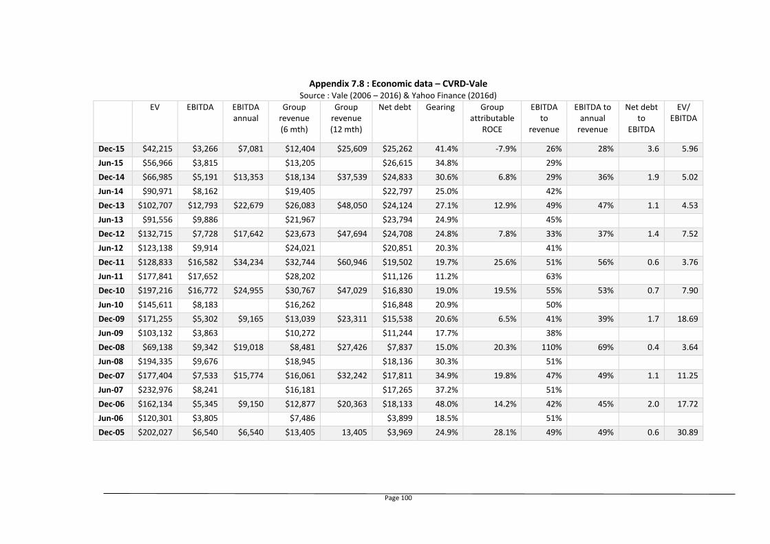
Page 100
Appendix 7.8 : Economic data – CVRD-Vale Source : Vale (2006 – 2016) & Yahoo Finance (2016d)
EV EBITDA EBITDA annual
Group revenue (6 mth)
Group revenue (12 mth)
Net debt Gearing Group attributable
ROCE
EBITDA to
revenue
EBITDA to annual
revenue
Net debt to
EBITDA
EV/ EBITDA
Dec-15 $42,215 $3,266 $7,081 $12,404 $25,609 $25,262 41.4% -7.9% 26% 28% 3.6 5.96
Jun-15 $56,966 $3,815 $13,205 $26,615 34.8% 29%
Dec-14 $66,985 $5,191 $13,353 $18,134 $37,539 $24,833 30.6% 6.8% 29% 36% 1.9 5.02
Jun-14 $90,971 $8,162 $19,405 $22,797 25.0% 42%
Dec-13 $102,707 $12,793 $22,679 $26,083 $48,050 $24,124 27.1% 12.9% 49% 47% 1.1 4.53
Jun-13 $91,556 $9,886 $21,967 $23,794 24.9% 45%
Dec-12 $132,715 $7,728 $17,642 $23,673 $47,694 $24,708 24.8% 7.8% 33% 37% 1.4 7.52
Jun-12 $123,138 $9,914 $24,021 $20,851 20.3% 41%
Dec-11 $128,833 $16,582 $34,234 $32,744 $60,946 $19,502 19.7% 25.6% 51% 56% 0.6 3.76
Jun-11 $177,841 $17,652 $28,202 $11,126 11.2% 63%
Dec-10 $197,216 $16,772 $24,955 $30,767 $47,029 $16,830 19.0% 19.5% 55% 53% 0.7 7.90
Jun-10 $145,611 $8,183 $16,262 $16,848 20.9% 50%
Dec-09 $171,255 $5,302 $9,165 $13,039 $23,311 $15,538 20.6% 6.5% 41% 39% 1.7 18.69
Jun-09 $103,132 $3,863 $10,272 $11,244 17.7% 38%
Dec-08 $69,138 $9,342 $19,018 $8,481 $27,426 $7,837 15.0% 20.3% 110% 69% 0.4 3.64
Jun-08 $194,335 $9,676 $18,945 $18,136 30.3% 51%
Dec-07 $177,404 $7,533 $15,774 $16,061 $32,242 $17,811 34.9% 19.8% 47% 49% 1.1 11.25
Jun-07 $232,976 $8,241 $16,181 $17,265 37.2% 51%
Dec-06 $162,134 $5,345 $9,150 $12,877 $20,363 $18,133 48.0% 14.2% 42% 45% 2.0 17.72
Jun-06 $120,301 $3,805 $7,486 $3,899 18.5% 51%
Dec-05 $202,027 $6,540 $6,540 $13,405 13,405 $3,969 24.9% 28.1% 49% 49% 0.6 30.89
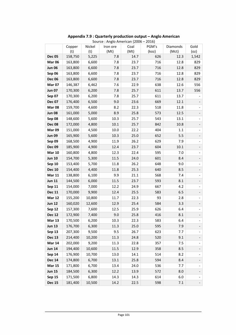
Page 101
Appendix 7.9 : Quarterly production output – Anglo American Source : Anglo American (2006 – 2016)
Copper (t)
Nickel (t)
Iron ore (Mt)
Coal (Mt)
PGM’s (koz)
Diamonds (Mct)
Gold (oz)
Dec 05 158,750 5,225 7.8 14.7 626 12.3 1,542
Mar 06 163,800 6,600 7.8 23.7 716 12.8 829
Jun 06 163,800 6,600 7.8 23.7 716 12.8 829
Sep 06 163,800 6,600 7.8 23.7 716 12.8 829
Dec 06 163,800 6,600 7.8 23.7 716 12.8 829
Mar 07 146,387 6,462 7.6 22.9 638 12.6 556
Jun 07 170,300 6,200 7.8 25.7 611 13.7 556
Sep 07 170,300 6,200 7.8 25.7 611 13.7 -
Dec 07 176,400 6,500 9.0 23.6 669 12.1 -
Mar 08 159,700 4,600 8.2 22.3 518 11.8 -
Jun 08 161,000 5,000 8.9 25.8 573 12.5 -
Sep 08 148,600 5,600 10.3 25.7 543 13.1 -
Dec 08 172,000 4,800 10.1 25.7 842 10.8 -
Mar 09 151,000 4,500 10.0 22.2 404 1.1 -
Jun 09 165,900 5,600 10.3 25.0 652 5.5 -
Sep 09 168,500 4,900 11.9 26.2 629 7.9 -
Dec 09 185,900 4,900 12.4 23.7 604 10.1 -
Mar 10 160,800 4,800 12.3 22.4 595 7.0 -
Jun 10 154,700 5,300 11.5 24.0 601 8.4 -
Sep 10 153,400 5,700 11.8 26.2 648 9.0 -
Dec 10 154,400 4,400 11.8 25.3 640 8.5 -
Mar 11 138,800 6,100 9.9 21.1 568 7.4 -
Jun 11 144,500 6,000 11.5 23.7 593 8.1 -
Sep 11 154,000 7,000 12.2 24.9 667 4.2 -
Dec 11 170,000 9,900 12.4 25.5 583 6.5 -
Mar 12 155,200 10,800 11.7 22.3 93 2.8 -
Jun 12 160,020 12,600 12.9 25.4 584 3.3 -
Sep 12 157,300 7,600 12.5 25.9 626 6.4 -
Dec 12 172,900 7,400 9.0 25.8 416 8.1 -
Mar 13 170,500 6,200 10.3 22.3 583 6.4 -
Jun 13 176,700 6,300 11.3 25.0 595 7.9 -
Sep 13 207,300 9,500 9.5 26.7 623 7.7 -
Dec 13 214,400 10,200 11.3 24.8 520 9.1 -
Mar 14 202,000 9,200 11.3 22.8 357 7.5 -
Jun 14 194,400 10,600 11.5 12.9 358 8.5 -
Sep 14 176,900 10,700 13.0 14.1 514 8.2 -
Dec 14 174,800 6,700 13.1 25.8 594 8.4 -
Mar 15 171,800 6,700 13.4 24.0 536 7.7 -
Jun 15 184,500 6,300 12.2 13.9 572 8.0 -
Sep 15 171,500 6,800 14.3 14.3 614 6.0 -
Dec 15 181,400 10,500 14.2 22.5 598 7.1 -

Page 102
Appendix 7.10 : Quarterly production output – BHP Billiton Source : BHP Billiton (2005 – 2015) & South 32 (2015)
Petroleum (Mbbl)
Aluminium (kt)
Base metals (kt)
Diamonds (kct)
Iron ore (Mt)
Met. coal (Mt)
Energy coal (Mt)
Dec-05 29 341 317 640 24.26 8.91 21.43
Mar-06 26 329 294 512 21.12 8.46 18.67
Jun-06 31 344 312 583 26.11 9.22 21.79
Sep-06 31 337 250 487 25.00 9.24 21.78
Dec-06 28 338 301 937 25.37 8.96 22.03
Mar-07 28 331 358 889 22.88 9.08 20.93
Jun-07 30 334 342 911 25.74 11.13 21.23
Sep-07 30 337 308 1,022 25.86 9.57 19.62
Dec-07 30 338 348 843 27.74 9.64 20.61
Mar-08 33 318 329 620 28.41 6.84 16.39
Jun-08 36 305 391 864 29.92 9.13 18.72
Sep-08 35 309 309 773 29.82 9.21 18.06
Dec-08 33 310 308 594 29.35 10.15 16.48
Mar-09 32 304 283 951 28.18 7.59 15.22
Jun-09 38 310 307 903 27.04 9.46 17.71
Sep-09 41 313 284 780 30.10 9.40 18.06
Dec-09 39 313 271 760 32.44 8.89 15.46
Mar-10 37 306 229 770 31.16 8.15 16.34
Jun-10 41 309 291 740 31.24 10.92 16.27
Sep-10 43 314 291 703 31.98 10.29 17.11
Dec-10 37 314 302 676 33.66 7.78 16.51
Mar-11 36 305 274 551 33.23 6.67 6.67
Jun-11 43 313 272 576 35.52 7.92 18.34
Sep-11 51 315 220 457 39.57 9.29 18.46
Dec-11 58 313 280 481 41.07 8.49 16.92
Mar-12 57 277 281 433 37.94 7.33 17.24
Jun-12 56 248 313 413 40.89 8.10 18.48
Sep-12 61 270 274 313 39.77 8.93 19.61
Dec-12 60 297 295 295 42.19 8.88 18.26
Mar-13 55 303 434 322 40.20 8.96 16.00
Jun-13 59 310 462 - 47.68 10.85 18.56
Sep-13 63 310 403 - 48.84 10.18 19.64
Dec-13 58 302 440 - 48.86 11.54 17.77
Mar-14 61 286 414 - 49.56 11.46 17.72
Jun-14 65 276 470 - 56.64 11.88 18.36
Sep-14 67 261 389 - 57.09 12.76 17.84
Dec-14 64 256 424 - 56.35 11.13 10.12
Mar-15 62 245 460 - 58.97 9.65 10.47
Jun-15 63 241 435 - 60.08 11.39 10.60
Sep-15 65 - 377 - 61.31 10.44 9.85
Dec-15 60 242 385 - 56.96 10.48 9.54
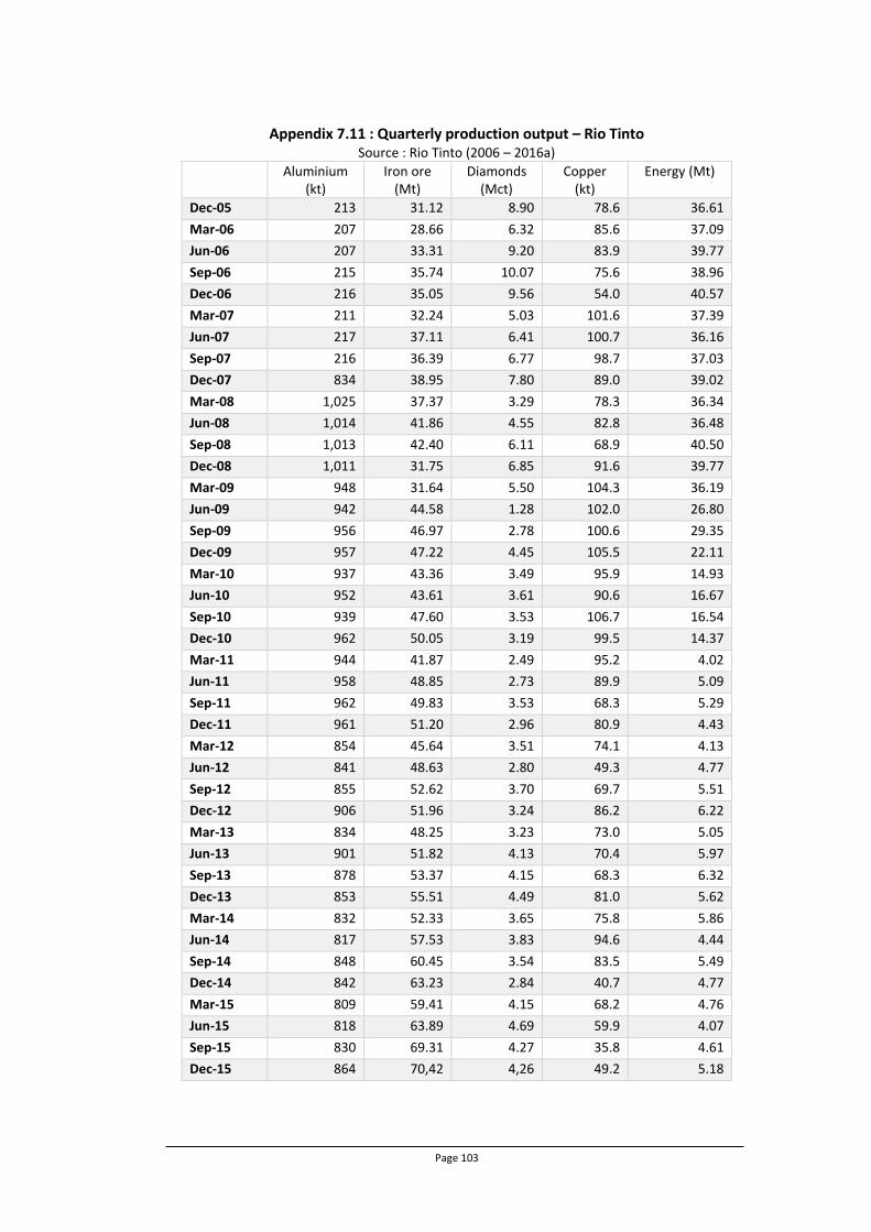
Page 103
Appendix 7.11 : Quarterly production output – Rio Tinto Source : Rio Tinto (2006 – 2016a)
Aluminium (kt)
Iron ore (Mt)
Diamonds (Mct)
Copper (kt)
Energy (Mt)
Dec-05 213 31.12 8.90 78.6 36.61
Mar-06 207 28.66 6.32 85.6 37.09
Jun-06 207 33.31 9.20 83.9 39.77
Sep-06 215 35.74 10.07 75.6 38.96
Dec-06 216 35.05 9.56 54.0 40.57
Mar-07 211 32.24 5.03 101.6 37.39
Jun-07 217 37.11 6.41 100.7 36.16
Sep-07 216 36.39 6.77 98.7 37.03
Dec-07 834 38.95 7.80 89.0 39.02
Mar-08 1,025 37.37 3.29 78.3 36.34
Jun-08 1,014 41.86 4.55 82.8 36.48
Sep-08 1,013 42.40 6.11 68.9 40.50
Dec-08 1,011 31.75 6.85 91.6 39.77
Mar-09 948 31.64 5.50 104.3 36.19
Jun-09 942 44.58 1.28 102.0 26.80
Sep-09 956 46.97 2.78 100.6 29.35
Dec-09 957 47.22 4.45 105.5 22.11
Mar-10 937 43.36 3.49 95.9 14.93
Jun-10 952 43.61 3.61 90.6 16.67
Sep-10 939 47.60 3.53 106.7 16.54
Dec-10 962 50.05 3.19 99.5 14.37
Mar-11 944 41.87 2.49 95.2 4.02
Jun-11 958 48.85 2.73 89.9 5.09
Sep-11 962 49.83 3.53 68.3 5.29
Dec-11 961 51.20 2.96 80.9 4.43
Mar-12 854 45.64 3.51 74.1 4.13
Jun-12 841 48.63 2.80 49.3 4.77
Sep-12 855 52.62 3.70 69.7 5.51
Dec-12 906 51.96 3.24 86.2 6.22
Mar-13 834 48.25 3.23 73.0 5.05
Jun-13 901 51.82 4.13 70.4 5.97
Sep-13 878 53.37 4.15 68.3 6.32
Dec-13 853 55.51 4.49 81.0 5.62
Mar-14 832 52.33 3.65 75.8 5.86
Jun-14 817 57.53 3.83 94.6 4.44
Sep-14 848 60.45 3.54 83.5 5.49
Dec-14 842 63.23 2.84 40.7 4.77
Mar-15 809 59.41 4.15 68.2 4.76
Jun-15 818 63.89 4.69 59.9 4.07
Sep-15 830 69.31 4.27 35.8 4.61
Dec-15 864 70,42 4,26 49.2 5.18
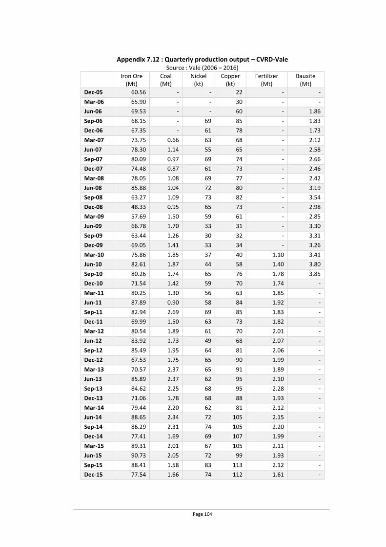
Page 104
Appendix 7.12 : Quarterly production output – CVRD-Vale Source : Vale (2006 – 2016)
Iron Ore (Mt)
Coal (Mt)
Nickel (kt)
Copper (kt)
Fertilizer (Mt)
Bauxite (Mt)
Dec-05 60.56 - - 22 - -
Mar-06 65.90 - - 30 - -
Jun-06 69.53 - - 60 - 1.86
Sep-06 68.15 - 69 85 - 1.83
Dec-06 67.35 - 61 78 - 1.73
Mar-07 73.75 0.66 63 68 - 2.12
Jun-07 78.30 1.14 55 65 - 2.58
Sep-07 80.09 0.97 69 74 - 2.66
Dec-07 74.48 0.87 61 73 - 2.46
Mar-08 78.05 1.08 69 77 - 2.42
Jun-08 85.88 1.04 72 80 - 3.19
Sep-08 63.27 1.09 73 82 - 3.54
Dec-08 48.33 0.95 65 73 - 2.98
Mar-09 57.69 1.50 59 61 - 2.85
Jun-09 66.78 1.70 33 31 - 3.30
Sep-09 63.44 1.26 30 32 - 3.31
Dec-09 69.05 1.41 33 34 - 3.26
Mar-10 75.86 1.85 37 40 1.10 3.41
Jun-10 82.61 1.87 44 58 1.40 3.80
Sep-10 80.26 1.74 65 76 1.78 3.85
Dec-10 71.54 1.42 59 70 1.74 -
Mar-11 80.25 1.30 56 63 1.85 -
Jun-11 87.89 0.90 58 84 1.92 -
Sep-11 82.94 2.69 69 85 1.83 -
Dec-11 69.99 1.50 63 73 1.82 -
Mar-12 80.54 1.89 61 70 2.01 -
Jun-12 83.92 1.73 49 68 2.07 -
Sep-12 85.49 1.95 64 81 2.06 -
Dec-12 67.53 1.75 65 90 1.99 -
Mar-13 70.57 2.37 65 91 1.89 -
Jun-13 85.89 2.37 62 95 2.10 -
Sep-13 84.62 2.25 68 95 2.28 -
Dec-13 71.06 1.78 68 88 1.93 -
Mar-14 79.44 2.20 62 81 2.12 -
Jun-14 88.65 2.34 72 105 2.15 -
Sep-14 86.29 2.31 74 105 2.20 -
Dec-14 77.41 1.69 69 107 1.99 -
Mar-15 89.31 2.01 67 105 2.11 -
Jun-15 90.73 2.05 72 99 1.93 -
Sep-15 88.41 1.58 83 113 2.12 -
Dec-15 77.54 1.66 74 112 1.61 -

Page 105
Appendix 7.13 : Bulk commodity and energy prices Source : World Bank (2016)

Page 106
Appendix 7.14 : Metals and diamonds prices Source : World Bank (2016)
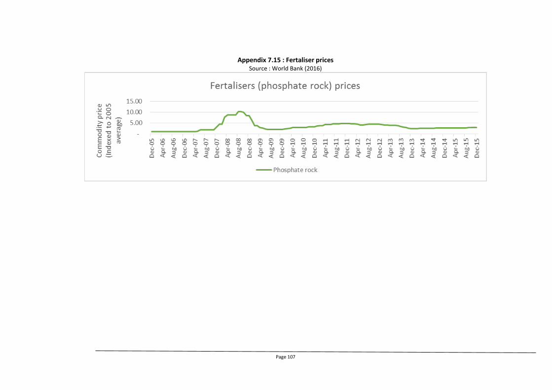
Page 107
Appendix 7.15 : Fertaliser prices Source : World Bank (2016)
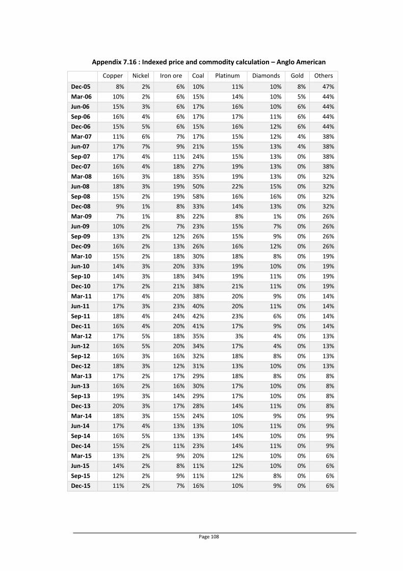
Page 108
Appendix 7.16 : Indexed price and commodity calculation – Anglo American
Copper Nickel Iron ore Coal Platinum Diamonds Gold Others
Dec-05 8% 2% 6% 10% 11% 10% 8% 47%
Mar-06 10% 2% 6% 15% 14% 10% 5% 44%
Jun-06 15% 3% 6% 17% 16% 10% 6% 44%
Sep-06 16% 4% 6% 17% 17% 11% 6% 44%
Dec-06 15% 5% 6% 15% 16% 12% 6% 44%
Mar-07 11% 6% 7% 17% 15% 12% 4% 38%
Jun-07 17% 7% 9% 21% 15% 13% 4% 38%
Sep-07 17% 4% 11% 24% 15% 13% 0% 38%
Dec-07 16% 4% 18% 27% 19% 13% 0% 38%
Mar-08 16% 3% 18% 35% 19% 13% 0% 32%
Jun-08 18% 3% 19% 50% 22% 15% 0% 32%
Sep-08 15% 2% 19% 58% 16% 16% 0% 32%
Dec-08 9% 1% 8% 33% 14% 13% 0% 32%
Mar-09 7% 1% 8% 22% 8% 1% 0% 26%
Jun-09 10% 2% 7% 23% 15% 7% 0% 26%
Sep-09 13% 2% 12% 26% 15% 9% 0% 26%
Dec-09 16% 2% 13% 26% 16% 12% 0% 26%
Mar-10 15% 2% 18% 30% 18% 8% 0% 19%
Jun-10 14% 3% 20% 33% 19% 10% 0% 19%
Sep-10 14% 3% 18% 34% 19% 11% 0% 19%
Dec-10 17% 2% 21% 38% 21% 11% 0% 19%
Mar-11 17% 4% 20% 38% 20% 9% 0% 14%
Jun-11 17% 3% 23% 40% 20% 11% 0% 14%
Sep-11 18% 4% 24% 42% 23% 6% 0% 14%
Dec-11 16% 4% 20% 41% 17% 9% 0% 14%
Mar-12 17% 5% 18% 35% 3% 4% 0% 13%
Jun-12 16% 5% 20% 34% 17% 4% 0% 13%
Sep-12 16% 3% 16% 32% 18% 8% 0% 13%
Dec-12 18% 3% 12% 31% 13% 10% 0% 13%
Mar-13 17% 2% 17% 29% 18% 8% 0% 8%
Jun-13 16% 2% 16% 30% 17% 10% 0% 8%
Sep-13 19% 3% 14% 29% 17% 10% 0% 8%
Dec-13 20% 3% 17% 28% 14% 11% 0% 8%
Mar-14 18% 3% 15% 24% 10% 9% 0% 9%
Jun-14 17% 4% 13% 13% 10% 11% 0% 9%
Sep-14 16% 5% 13% 13% 14% 10% 0% 9%
Dec-14 15% 2% 11% 23% 14% 11% 0% 9%
Mar-15 13% 2% 9% 20% 12% 10% 0% 6%
Jun-15 14% 2% 8% 11% 12% 10% 0% 6%
Sep-15 12% 2% 9% 11% 12% 8% 0% 6%
Dec-15 11% 2% 7% 16% 10% 9% 0% 6%

Page 109
Appendix 7.17 : Indexed price and commodity calculation – BHP Billiton
Petroleum Aluminium Base metals
Diamonds Iron ore
Met. coal
Energy coal
Others
Dec-05 19% 22% 16% 5% 16% 8% 11% 2%
Mar-06 20% 27% 20% 4% 15% 7% 9% 1%
Jun-06 26% 31% 31% 5% 18% 7% 12% 1%
Sep-06 26% 29% 27% 4% 18% 7% 12% 1%
Dec-06 20% 32% 30% 8% 19% 7% 11% 1%
Mar-07 20% 32% 29% 8% 20% 6% 12% 0%
Jun-07 25% 32% 36% 8% 26% 9% 13% 0%
Sep-07 28% 30% 33% 10% 34% 9% 14% 0%
Dec-07 33% 28% 35% 9% 53% 12% 18% 0%
Mar-08 39% 30% 36% 7% 57% 14% 20% 1%
Jun-08 54% 31% 46% 10% 59% 25% 28% 1%
Sep-08 50% 30% 33% 9% 51% 25% 31% 1%
Dec-08 23% 19% 17% 7% 23% 18% 16% 1%
Mar-09 17% 14% 13% 11% 21% 7% 12% 3%
Jun-09 28% 16% 20% 10% 18% 8% 13% 3%
Sep-09 35% 20% 23% 9% 27% 11% 14% 3%
Dec-09 36% 22% 25% 9% 33% 11% 13% 3%
Mar-10 36% 23% 23% 9% 42% 12% 17% 1%
Jun-10 40% 22% 28% 9% 52% 18% 17% 1%
Sep-10 40% 23% 29% 8% 46% 15% 17% 1%
Dec-10 40% 25% 36% 8% 54% 12% 19% 1%
Mar-11 44% 26% 37% 7% 62% 16% 9% 0%
Jun-11 59% 28% 35% 7% 65% 18% 24% 0%
Sep-11 66% 26% 27% 6% 72% 19% 24% 0%
Dec-11 74% 23% 29% 6% 60% 15% 21% 0%
Mar-12 79% 21% 32% 6% 56% 11% 21% 0%
Jun-12 72% 17% 34% 5% 59% 13% 19% 0%
Sep-12 78% 18% 29% 4% 46% 11% 19% 0%
Dec-12 76% 20% 32% 4% 53% 10% 17% 0%
Mar-13 72% 21% 48% 4% 62% 11% 16% 1%
Jun-13 73% 20% 46% 0% 62% 11% 17% 1%
Sep-13 83% 19% 40% 0% 67% 10% 16% 1%
Dec-13 75% 18% 44% 0% 68% 11% 16% 1%
Mar-14 78% 17% 40% 0% 62% 10% 15% 0%
Jun-14 85% 17% 44% 0% 60% 9% 14% 0%
Sep-14 84% 18% 38% 0% 54% 10% 13% 0%
Dec-14 59% 17% 39% 0% 43% 9% 7% 0%
Mar-15 39% 15% 37% 0% 39% 7% 7% 2%
Jun-15 47% 15% 37% 0% 36% 7% 7% 2%
Sep-15 39% 0% 28% 0% 35% 6% 6% 2%
Dec-15 31% 12% 26% 0% 28% 6% 5% 2%

Page 110
Appendix 7.18 : Indexed price and commodity calculation – Rio Tinto
Aluminium Iron Ore Diamonds Copper Energy Others
Dec-05 13% 27% 17% 23% 19% 1%
Mar-06 16% 25% 12% 34% 19% 1%
Jun-06 18% 30% 18% 49% 22% 1%
Sep-06 17% 33% 20% 47% 21% 1%
Dec-06 19% 33% 21% 31% 20% 1%
Mar-07 19% 35% 12% 49% 21% 0%
Jun-07 20% 48% 15% 62% 22% 0%
Sep-07 18% 60% 16% 61% 27% 0%
Dec-07 67% 94% 20% 52% 35% 0%
Mar-08 92% 94% 9% 49% 44% 1%
Jun-08 97% 105% 13% 56% 54% 1%
Sep-08 92% 92% 19% 43% 71% 1%
Dec-08 60% 31% 21% 29% 40% 1%
Mar-09 42% 29% 17% 29% 28% 13%
Jun-09 46% 38% 4% 38% 19% 13%
Sep-09 57% 54% 8% 48% 22% 13%
Dec-09 63% 60% 13% 57% 18% 13%
Mar-10 66% 74% 10% 56% 15% 8%
Jun-10 65% 91% 11% 51% 18% 8%
Sep-10 64% 86% 11% 62% 17% 8%
Dec-10 74% 102% 10% 69% 17% 8%
Mar-11 77% 98% 8% 74% 6% 8%
Jun-11 82% 112% 9% 67% 7% 8%
Sep-11 75% 115% 12% 49% 7% 8%
Dec-11 66% 94% 10% 49% 5% 8%
Mar-12 61% 85% 12% 50% 5% 8%
Jun-12 54% 89% 9% 31% 5% 8%
Sep-12 54% 77% 12% 43% 5% 8%
Dec-12 59% 82% 10% 55% 6% 8%
Mar-13 54% 94% 10% 47% 5% 1%
Jun-13 54% 85% 13% 41% 6% 1%
Sep-13 51% 93% 13% 39% 5% 1%
Dec-13 49% 98% 14% 47% 5% 1%
Mar-14 46% 83% 11% 43% 5% 0%
Jun-14 48% 77% 12% 52% 3% 0%
Sep-14 55% 72% 11% 47% 4% 0%
Dec-14 54% 62% 9% 22% 3% 0%
Mar-15 48% 49% 13% 32% 3% 0%
Jun-15 47% 49% 15% 29% 3% 0%
Sep-15 43% 50% 13% 15% 3% 0%
Dec-15 42% 43% 13% 19% 3% 0%

Page 111
Appendix 7.19 : Indexed price and commodity calculation – CVRD-Vale
Iron ore Coal Nickel Copper Fertilizer Bauxite Others
Dec-05 29% 0% 0% 3% 0% 11% 9%
Mar-06 32% 0% 0% 1% 0% 11% 7%
Jun-06 35% 0% 0% 3% 0% 11% 7%
Sep-06 35% 0% 27% 4% 0% 7% 7%
Dec-06 36% 0% 27% 4% 0% 5% 7%
Mar-07 45% 0% 34% 3% 0% 4% 5%
Jun-07 57% 1% 35% 3% 0% 5% 5%
Sep-07 74% 1% 28% 4% 0% 5% 5%
Dec-07 102% 1% 24% 3% 0% 4% 5%
Mar-08 111% 1% 27% 4% 0% 5% 5%
Jun-08 121% 1% 25% 4% 0% 7% 5%
Sep-08 78% 2% 18% 4% 0% 7% 5%
Dec-08 27% 1% 9% 2% 0% 4% 5%
Mar-09 30% 1% 8% 1% 0% 3% 6%
Jun-09 32% 1% 6% 1% 0% 4% 6%
Sep-09 41% 1% 7% 1% 0% 4% 6%
Dec-09 50% 1% 8% 1% 0% 5% 6%
Mar-10 74% 2% 10% 2% 4% 5% 4%
Jun-10 97% 2% 13% 3% 6% 6% 4%
Sep-10 82% 2% 18% 4% 8% 6% 4%
Dec-10 83% 1% 18% 4% 8% 0% 4%
Mar-11 106% 2% 20% 4% 10% 0% 4%
Jun-11 114% 1% 19% 5% 12% 0% 4%
Sep-11 108% 3% 20% 5% 12% 0% 4%
Dec-11 73% 2% 15% 4% 12% 0% 4%
Mar-12 84% 2% 16% 4% 13% 0% 5%
Jun-12 87% 2% 11% 4% 13% 0% 5%
Sep-12 71% 2% 14% 4% 13% 0% 5%
Dec-12 60% 2% 15% 5% 12% 0% 5%
Mar-13 77% 2% 15% 5% 11% 0% 2%
Jun-13 80% 2% 12% 4% 12% 0% 2%
Sep-13 83% 2% 13% 4% 11% 0% 2%
Dec-13 71% 2% 12% 4% 7% 0% 2%
Mar-14 71% 2% 12% 4% 7% 0% 3%
Jun-14 67% 2% 18% 5% 8% 0% 3%
Sep-14 58% 2% 18% 5% 8% 0% 3%
Dec-14 43% 1% 15% 5% 8% 0% 3%
Mar-15 42% 1% 13% 4% 8% 0% 1%
Jun-15 39% 1% 12% 4% 7% 0% 1%
Sep-15 36% 1% 12% 4% 8% 0% 1%
Dec-15 27% 1% 9% 4% 7% 0% 1%
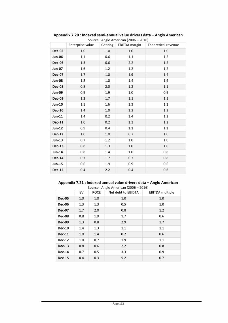
Page 112
Appendix 7.20 : Indexed semi-annual value drivers data – Anglo American Source : Anglo American (2006 – 2016)
Enterprise value Gearing EBITDA margin Theoretical revenue
Dec-05 1.0 1.0 1.0 1.0
Jun-06 1.1 0.6 1.1 1.2
Dec-06 1.3 0.6 2.2 1.2
Jun-07 1.6 1.2 1.2 1.2
Dec-07 1.7 1.0 1.9 1.4
Jun-08 1.8 1.0 1.4 1.6
Dec-08 0.8 2.0 1.2 1.1
Jun-09 0.9 1.9 1.0 0.9
Dec-09 1.3 1.7 1.1 1.1
Jun-10 1.1 1.6 1.3 1.2
Dec-10 1.4 1.0 1.3 1.3
Jun-11 1.4 0.2 1.4 1.3
Dec-11 1.0 0.2 1.3 1.2
Jun-12 0.9 0.4 1.1 1.1
Dec-12 1.0 1.0 0.7 1.0
Jun-13 0.7 1.2 1.0 1.0
Dec-13 0.8 1.3 1.0 1.0
Jun-14 0.8 1.4 1.0 0.8
Dec-14 0.7 1.7 0.7 0.8
Jun-15 0.6 1.9 0.9 0.6
Dec-15 0.4 2.2 0.4 0.6
Appendix 7.21 : Indexed annual value drivers data – Anglo American
Source : Anglo American (2006 – 2016) EV ROCE Net debt to EBIDTA EBITDA multiple
Dec-05 1.0 1.0 1.0 1.0
Dec-06 1.3 1.3 0.5 1.0
Dec-07 1.7 2.0 0.8 1.2
Dec-08 0.8 1.9 1.7 0.6
Dec-09 1.3 0.8 2.9 1.7
Dec-10 1.4 1.3 1.1 1.1
Dec-11 1.0 1.4 0.2 0.6
Dec-12 1.0 0.7 1.9 1.1
Dec-13 0.8 0.6 2.2 0.8
Dec-14 0.7 0.5 3.3 0.9
Dec-15 0.4 0.3 5.2 0.7
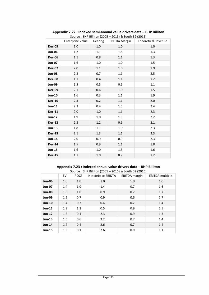
Page 113
Appendix 7.22 : Indexed semi-annual value drivers data – BHP Billiton Source : BHP Billiton (2005 – 2015) & South 32 (2015)
Enterprise Value Gearing EBITDA Margin Theoretical Revenue
Dec-05 1.0 1.0 1.0 1.0
Jun-06 1.2 1.1 1.8 1.3
Dec-06 1.1 0.8 1.1 1.3
Jun-07 1.6 1.0 1.0 1.5
Dec-07 2.0 1.1 1.0 1.9
Jun-08 2.2 0.7 1.1 2.5
Dec-08 1.1 0.4 1.1 1.2
Jun-09 1.5 0.5 0.5 1.1
Dec-09 2.1 0.6 1.0 1.5
Jun-10 1.6 0.3 1.1 1.9
Dec-10 2.3 0.2 1.1 2.0
Jun-11 2.3 0.4 1.5 2.4
Dec-11 2.0 1.0 1.1 2.3
Jun-12 1.9 1.0 1.5 2.2
Dec-12 2.3 1.2 0.9 2.1
Jun-13 1.8 1.1 1.0 2.3
Dec-13 2.1 1.3 1.1 2.3
Jun-14 2.0 0.9 0.9 2.3
Dec-14 1.5 0.9 1.1 1.8
Jun-15 1.6 1.0 1.5 1.6
Dec-15 1.1 1.0 0.7 1.2
Appendix 7.23 : Indexed annual value drivers data – BHP Billiton
Source : BHP Billiton (2005 – 2015) & South 32 (2015) EV ROCE Net debt to EBIDTA EBITDA margin EBITDA multiple
Jun-06 1.0 1.0 1.0 1.0 1.0
Jun-07 1.4 1.0 1.4 0.7 1.6
Jun-08 1.8 1.0 0.9 0.7 1.7
Jun-09 1.2 0.7 0.9 0.6 1.7
Jun-10 1.4 0.7 0.4 0.7 1.4
Jun-11 1.9 1.2 0.5 0.9 1.5
Jun-12 1.6 0.4 2.3 0.9 1.3
Jun-13 1.5 0.6 3.2 0.7 1.4
Jun-14 1.7 0.4 2.6 0.7 1.4
Jun-15 1.3 0.1 2.6 0.9 1.1

Page 114
Appendix 7.24 : Indexed semi-annual value drivers data – Rio Tinto Source : Rio Tinto (2006 – 2016a)
Enterprise value Gearing Theoretical revenue
Dec-05 1.0 1.0 1.0
Jun-06 1.1 1.8 1.4
Dec-06 1.1 1.5 1.3
Jun-07 1.6 1.5 1.7
Dec-07 2.9 8.2 2.7
Jun-08 3.1 7.2 3.3
Dec-08 1.2 8.2 1.8
Jun-09 1.7 8.7 1.6
Dec-09 2.1 3.8 2.2
Jun-10 1.8 2.6 2.4
Dec-10 2.6 0.8 2.8
Jun-11 2.8 1.4 2.8
Dec-11 1.9 1.6 2.3
Jun-12 2.0 3.0 2.0
Dec-12 2.3 3.2 2.2
Jun-13 1.8 3.7 2.0
Dec-13 2.2 3.3 2.1
Jun-14 2.0 2.4 1.9
Dec-14 1.8 2.4 1.5
Jun-15 1.6 2.8 1.4
Dec-15 1.3 3.1 1.2
Appendix 7.25 : Indexed annual value drivers data – Rio Tinto Source : Rio Tinto (2006 – 2016a)
EV ROCE Net debt to EBIDTA EBITDA margin EBITDA multiple
Dec-05 1.0 1.0 1.0 1.0 1.0
Dec-06 1.1 1.2 1.4 1.1 0.9
Dec-07 2.9 0.4 24.6 0.9 2.1
Dec-08 1.2 0.5 12.0 0.9 0.5
Dec-09 2.1 0.3 9.8 0.7 1.5
Dec-10 2.6 0.7 1.2 1.0 1.0
Dec-11 1.9 0.4 2.2 0.9 0.6
Dec-12 2.3 (0.1) 7.1 0.8 1.1
Dec-13 2.2 0.3 6.4 0.8 1.0
Dec-14 1.8 0.4 4.9 0.8 0.9
Dec-15 1.3 0.2 8.5 0.7 1.0

Page 115
Appendix 7.26 : Indexed semi-annual value drivers data – CVRD-Vale Source : Vale (2006 - 2016)
Enterprise value Gearing Theoretical revenue
Dec-05 - - -
Jun-06 1.0 1.0 1.0
Dec-06 1.3 2.6 1.4
Jun-07 1.9 2.0 1.9
Dec-07 1.5 1.9 2.5
Jun-08 1.6 1.6 2.9
Dec-08 0.6 0.8 0.9
Jun-09 0.9 1.0 0.9
Dec-09 1.4 1.1 1.3
Jun-10 1.2 1.1 2.3
Dec-10 1.6 1.0 2.1
Jun-11 1.5 0.6 2.8
Dec-11 1.1 1.1 2.0
Jun-12 1.0 1.1 2.2
Dec-12 1.1 1.3 1.8
Jun-13 0.8 1.3 2.0
Dec-13 0.9 1.5 1.8
Jun-14 0.8 1.4 1.8
Dec-14 0.6 1.7 1.3
Jun-15 0.5 1.9 1.2
Dec-15 0.4 2.2 0.9
Appendix 7.27 : Indexed annual value drivers data – CVRD-Vale
Source : Vale (2006 - 2016) EV ROCE Net debt to EBIDTA EBITDA margin EBITDA multiple
Dec-05 - - - - -
Dec-06 1.0 1.0 1.0 1.0 1.0
Dec-07 1.1 1.4 0.6 1.1 0.6
Dec-08 0.4 1.4 0.2 1.5 0.2
Dec-09 1.1 0.5 0.9 0.9 1.1
Dec-10 1.2 1.4 0.3 1.2 0.4
Dec-11 0.8 1.8 0.3 1.3 0.2
Dec-12 0.8 0.5 0.7 0.8 0.4
Dec-13 0.6 0.9 0.5 1.1 0.3
Dec-14 0.4 0.5 0.9 0.8 0.3
Dec-15 0.3 (0.6) 1.8 0.6 0.3