analysis of flow through cylindrical packed beds …...analysis of flow through cylindrical packed...
TRANSCRIPT
Analysis of flow through cylindrical packed beds with small cylinder diameter
to particle diameter ratios.
WJS Van der Merwe
Dissertation submitted in fulfilment of the requirements for the degree Master in Nuclear Engineering at the Potchefstroom Campus of the North-West University
Supervisor: Prof CG du Toit
Co-Supervisor: Dr J-H Kruger
May 2014
Abstract
The wall effect is known to present difficulties when attempting to predict the pressure dropover randomly packed beds. The Nuclear Safety Standard Commission, “Kerntechnischer Auss-chuss” (KTA), made considerable efforts to develop an equation which predicts the pressuredrop over cylindrical randomly packed beds consisting of mono-sized spheres. The KTA wasable to estimate a limiting line, which defines the region for which the wall effect is negligible,however the theoretical basis for this line is unclear. The goal of this investigation was todetermine the validity of the KTA limiting line, using an explicit approach.
Packed beds were generated using Discrete Element Modelling (DEM), and the flow throughthe beds simulated using Computational Fluid Dynamics (CFD). STAR-CCM+ R© was used forboth DEM and CFD operations, and the methods developed for this explicit approach werevalidated with empirical data. The KTA correlation predictions for friction factors were com-pared with the CFD results, as well as the predictions from a few other correlations.
The KTA correlation predictions for friction factors did not correspond well with the CFDresults at low aspect ratios and low modified Reynolds numbers, due to the influence of thewall effect. The KTA limiting line was found to be valid, but not exact. A new limiting line forthe KTA correlation was suggested, however the new limiting line improved little on the existingline and was the result of some major assumptions. In order to improve the determination ofthe position of the KTA limiting line further, criteria need to be established which determinehow small the error in predicted friction factor must be before the KTA correlation can beaccepted as accurate.
Keywords: Randomly packed beds; Spherical particles; Low aspect ratios; Pressure drop;Porosity; Wall effect; DEM; CFD; STAR-CCM+ R©.
I
Declaration
I, Wian Johannes Stephanus van der Merwe (Identity Number: 890626 5083 089), hereby declarethe work contained in this dissertation to be my own. All information which has been gainedfrom various journal articles, text books or other sources has been referenced accordingly.
Mr. W.J.S. van der Merwe Date
II

Acknowledgements
First and foremost I humbly thank my heavenly Father for His unending love, support andstrength. Without Him this project would not have been possible.
I would like to express my gratitude to all those who have supported me during this study.My sincere thanks goes to my study leaders, Prof. C.G. (Jat) du Toit and Dr. J-H. Kruger,whose advice and guidance lead me during every step of this study. Prof. Jat, whose mad-dening attention to detail drove me to finally learn the difference between “compared to” and“compared with”, taught me the value of research and also encouraged me to pursue a Ph.D.internationally. For that, I am extremely grateful. It has been a pleasure and a privilege towork under these insightful and knowledgeable leaders.
I also thank my friend and colleague, Mr. Lambert H. Fick, who helped me through the diffi-culties of this study and motivated me to always keep a positive outlook. I will be ever gratefulfor his friendship and support.
Finally I would like to thank my parents and my brother for their love, encouragement, patienceand advice during these past two years. Though they might not have fully understood what thisstudy entailed, they were always on hand to help me through the rough times. This study wouldnot have been possible without them, and my gratitude for their unending support cannot beexpressed in words.
This work is based upon research supported by the South African Research Chairs Initiativeof the Department of Science and Technology and National Research Foundation. Any opin-ions, findings and conclusions or recommendations expressed in this material are those of theauthor(s) and therefore the NRF and DST do not accept any liability with regard thereto.
III
Contents
Abstract I
Declaration II
Acknowledgements III
Table Of Contents IV
List Of Figures VII
List Of Tables IX
Nomenclature X
1 Introduction 11.1 Background . . . . . . . . . . . . . . . . . . . . . . . . . . . . . . . . . . . . . . 11.2 Problem statement . . . . . . . . . . . . . . . . . . . . . . . . . . . . . . . . . . 31.3 Objectives . . . . . . . . . . . . . . . . . . . . . . . . . . . . . . . . . . . . . . . 31.4 Methodology . . . . . . . . . . . . . . . . . . . . . . . . . . . . . . . . . . . . . 31.5 Overview of document . . . . . . . . . . . . . . . . . . . . . . . . . . . . . . . . 3
2 Literature survey 52.1 Packed bed definition . . . . . . . . . . . . . . . . . . . . . . . . . . . . . . . . . 52.2 Packed bed structure . . . . . . . . . . . . . . . . . . . . . . . . . . . . . . . . . 6
2.2.1 Aspect ratios . . . . . . . . . . . . . . . . . . . . . . . . . . . . . . . . . 62.2.2 Porosity . . . . . . . . . . . . . . . . . . . . . . . . . . . . . . . . . . . . 62.2.3 Packing . . . . . . . . . . . . . . . . . . . . . . . . . . . . . . . . . . . . 72.2.4 Voronoi tessellation . . . . . . . . . . . . . . . . . . . . . . . . . . . . . . 82.2.5 Coordination number . . . . . . . . . . . . . . . . . . . . . . . . . . . . . 92.2.6 Contact angles between adjacent particles . . . . . . . . . . . . . . . . . 10
2.3 Porosity variations . . . . . . . . . . . . . . . . . . . . . . . . . . . . . . . . . . 102.3.1 Porosity variations in the radial direction . . . . . . . . . . . . . . . . . . 102.3.2 Effect of cylinder wall on porosity . . . . . . . . . . . . . . . . . . . . . . 122.3.3 Porosity variations in the axial direction . . . . . . . . . . . . . . . . . . 132.3.4 Porosity variations as a function of the aspect ratio . . . . . . . . . . . . 132.3.5 Conclusions on porosity . . . . . . . . . . . . . . . . . . . . . . . . . . . 14
2.4 The wall effect . . . . . . . . . . . . . . . . . . . . . . . . . . . . . . . . . . . . . 152.5 Prediction of pressure drop . . . . . . . . . . . . . . . . . . . . . . . . . . . . . . 16
IV
2.5.1 Background . . . . . . . . . . . . . . . . . . . . . . . . . . . . . . . . . . 162.5.2 Types of equations . . . . . . . . . . . . . . . . . . . . . . . . . . . . . . 172.5.3 The KTA correlation . . . . . . . . . . . . . . . . . . . . . . . . . . . . . 182.5.4 The Eisfeld and Schnitzlein correlation . . . . . . . . . . . . . . . . . . . 192.5.5 The Wentz and Thodos correlation . . . . . . . . . . . . . . . . . . . . . 192.5.6 Final remarks . . . . . . . . . . . . . . . . . . . . . . . . . . . . . . . . . 20
2.6 Discrete Element Modelling . . . . . . . . . . . . . . . . . . . . . . . . . . . . . 202.7 Computational Fluid Dynamics . . . . . . . . . . . . . . . . . . . . . . . . . . . 21
2.7.1 CFD and packed beds . . . . . . . . . . . . . . . . . . . . . . . . . . . . 212.7.2 Meshing packed beds . . . . . . . . . . . . . . . . . . . . . . . . . . . . . 222.7.3 Contact treatment . . . . . . . . . . . . . . . . . . . . . . . . . . . . . . 232.7.4 Turbulence models . . . . . . . . . . . . . . . . . . . . . . . . . . . . . . 242.7.5 Inlet boundary condition . . . . . . . . . . . . . . . . . . . . . . . . . . . 252.7.6 Inlet and outlet regions . . . . . . . . . . . . . . . . . . . . . . . . . . . . 262.7.7 Pressure drop measurement . . . . . . . . . . . . . . . . . . . . . . . . . 27
2.8 Summary . . . . . . . . . . . . . . . . . . . . . . . . . . . . . . . . . . . . . . . 27
3 Modelling theory 293.1 Discrete Element Modelling . . . . . . . . . . . . . . . . . . . . . . . . . . . . . 29
3.1.1 Momentum balance . . . . . . . . . . . . . . . . . . . . . . . . . . . . . . 293.1.2 Contact force modelling . . . . . . . . . . . . . . . . . . . . . . . . . . . 30
3.2 Computational Fluid Dynamics . . . . . . . . . . . . . . . . . . . . . . . . . . . 313.2.1 Transport equations . . . . . . . . . . . . . . . . . . . . . . . . . . . . . 313.2.2 Finite volume method . . . . . . . . . . . . . . . . . . . . . . . . . . . . 323.2.3 Turbulence . . . . . . . . . . . . . . . . . . . . . . . . . . . . . . . . . . 333.2.4 Mesh generation . . . . . . . . . . . . . . . . . . . . . . . . . . . . . . . 34
3.3 Summary . . . . . . . . . . . . . . . . . . . . . . . . . . . . . . . . . . . . . . . 35
4 Methodology 364.1 DEM simulation setup . . . . . . . . . . . . . . . . . . . . . . . . . . . . . . . . 36
4.1.1 Geometry and boundaries . . . . . . . . . . . . . . . . . . . . . . . . . . 364.1.2 Particle injection . . . . . . . . . . . . . . . . . . . . . . . . . . . . . . . 364.1.3 Mesh continua . . . . . . . . . . . . . . . . . . . . . . . . . . . . . . . . . 374.1.4 Physics continua . . . . . . . . . . . . . . . . . . . . . . . . . . . . . . . 374.1.5 Material . . . . . . . . . . . . . . . . . . . . . . . . . . . . . . . . . . . . 384.1.6 Stopping criteria . . . . . . . . . . . . . . . . . . . . . . . . . . . . . . . 38
4.2 CFD simulation setup . . . . . . . . . . . . . . . . . . . . . . . . . . . . . . . . 394.2.1 Geometry . . . . . . . . . . . . . . . . . . . . . . . . . . . . . . . . . . . 394.2.2 Boundaries . . . . . . . . . . . . . . . . . . . . . . . . . . . . . . . . . . 404.2.3 Mesh continua . . . . . . . . . . . . . . . . . . . . . . . . . . . . . . . . . 404.2.4 Physics continua . . . . . . . . . . . . . . . . . . . . . . . . . . . . . . . 414.2.5 Solvers and stopping criteria . . . . . . . . . . . . . . . . . . . . . . . . . 41
4.3 Reference bed . . . . . . . . . . . . . . . . . . . . . . . . . . . . . . . . . . . . . 414.4 Working fluid . . . . . . . . . . . . . . . . . . . . . . . . . . . . . . . . . . . . . 424.5 Mesh independence study . . . . . . . . . . . . . . . . . . . . . . . . . . . . . . 42
4.5.1 Parameters used for mesh quality analysis . . . . . . . . . . . . . . . . . 434.5.2 Meshing model and contact treatment . . . . . . . . . . . . . . . . . . . 44
V
4.5.3 Contact area . . . . . . . . . . . . . . . . . . . . . . . . . . . . . . . . . 454.5.4 Mesh density . . . . . . . . . . . . . . . . . . . . . . . . . . . . . . . . . 464.5.5 Wall treatment and y+ values . . . . . . . . . . . . . . . . . . . . . . . . 47
4.6 Turbulence modelling . . . . . . . . . . . . . . . . . . . . . . . . . . . . . . . . . 484.7 Inlet boundary conditions . . . . . . . . . . . . . . . . . . . . . . . . . . . . . . 494.8 Packed bed length . . . . . . . . . . . . . . . . . . . . . . . . . . . . . . . . . . 494.9 Pressure drop measurement . . . . . . . . . . . . . . . . . . . . . . . . . . . . . 514.10 Summary . . . . . . . . . . . . . . . . . . . . . . . . . . . . . . . . . . . . . . . 52
5 Results 535.1 Analysis of DEM generated beds . . . . . . . . . . . . . . . . . . . . . . . . . . 53
5.1.1 Particle overlaps . . . . . . . . . . . . . . . . . . . . . . . . . . . . . . . 545.1.2 Porosity and structure . . . . . . . . . . . . . . . . . . . . . . . . . . . . 54
5.2 Computational resources . . . . . . . . . . . . . . . . . . . . . . . . . . . . . . . 565.3 Validation . . . . . . . . . . . . . . . . . . . . . . . . . . . . . . . . . . . . . . . 59
5.3.1 Wentz and Thodos . . . . . . . . . . . . . . . . . . . . . . . . . . . . . . 605.3.2 Hassan and Kang . . . . . . . . . . . . . . . . . . . . . . . . . . . . . . . 62
5.4 Pressure drop . . . . . . . . . . . . . . . . . . . . . . . . . . . . . . . . . . . . . 635.5 Friction factor . . . . . . . . . . . . . . . . . . . . . . . . . . . . . . . . . . . . . 645.6 Summary . . . . . . . . . . . . . . . . . . . . . . . . . . . . . . . . . . . . . . . 68
6 Conclusions 696.1 Conclusions . . . . . . . . . . . . . . . . . . . . . . . . . . . . . . . . . . . . . . 696.2 Recommendations . . . . . . . . . . . . . . . . . . . . . . . . . . . . . . . . . . . 70
Bibliography 72
VI

List of Figures
1.1 Lower limit of the KTA correlation: the KTA limiting line. . . . . . . . . . . . . 2
2.1 Types of layers formed by spherical particles. . . . . . . . . . . . . . . . . . . . . 72.2 Packing structures. . . . . . . . . . . . . . . . . . . . . . . . . . . . . . . . . . . 82.3 Schematic illustration of Voronoi tessellation. . . . . . . . . . . . . . . . . . . . . 92.4 Radial porosity variation. . . . . . . . . . . . . . . . . . . . . . . . . . . . . . . 112.5 Distribution of the centre coordinates of the spheres. . . . . . . . . . . . . . . . 122.6 Average bed porosity as a function of the aspect ratio. . . . . . . . . . . . . . . 142.7 Predictions of bulk porosities. . . . . . . . . . . . . . . . . . . . . . . . . . . . . 152.8 Schematic of a packed bed with a typical velocity profile. . . . . . . . . . . . . . 162.9 Schematic of the mesh between a particle and the cylinder wall. . . . . . . . . . 222.10 Artificial gap between two spheres. . . . . . . . . . . . . . . . . . . . . . . . . . 242.11 Typical velocity profiles in a cylindrical pipe. . . . . . . . . . . . . . . . . . . . . 262.12 Schematic of a packed bed domain. . . . . . . . . . . . . . . . . . . . . . . . . . 272.13 Profile of pressure as a function of the axial distance. . . . . . . . . . . . . . . . 27
4.1 Schematic of curvature deviation. . . . . . . . . . . . . . . . . . . . . . . . . . . 374.2 Examples of finished DEM simulations. . . . . . . . . . . . . . . . . . . . . . . . 394.3 Examples of domains created for CFD simulations. . . . . . . . . . . . . . . . . 394.4 Illustration of the regions specified for the CFD simulations. . . . . . . . . . . . 404.5 Reference bed used for the development of the methodology. . . . . . . . . . . . 424.6 Illustration of a skewness angle between cells. . . . . . . . . . . . . . . . . . . . 434.7 Schematic illustration of cell quality. . . . . . . . . . . . . . . . . . . . . . . . . 434.8 Examples of contact points between surfaces. . . . . . . . . . . . . . . . . . . . . 444.9 Mesh structure at a contact point between two particles. . . . . . . . . . . . . . 454.10 Illustration of a contact point between two particles. . . . . . . . . . . . . . . . 454.11 Mesh structure at a contact point between two particles. . . . . . . . . . . . . . 464.12 Pressure drop vs. the contact point fillet radius and mesh density. . . . . . . . . 474.13 Mesh structure in the reference bed. . . . . . . . . . . . . . . . . . . . . . . . . . 474.14 Pressure drop over the reference bed using LES. . . . . . . . . . . . . . . . . . . 494.15 Comparison between the k − ε model and LES. . . . . . . . . . . . . . . . . . . 504.16 Pressure drop over the reference bed vs. the axial length. . . . . . . . . . . . . . 504.17 Change in pressure vs. the dimensionless axial coordinate. . . . . . . . . . . . . 51
5.1 Quality analysis of the DEM generated packed beds. . . . . . . . . . . . . . . . 545.2 Bulk porosities of the DEM generated beds. . . . . . . . . . . . . . . . . . . . . 555.3 Illustration of the bulk porosities including and excluding the length effect. . . . 565.4 Porosity variation in the axial direction of the DEM generated beds. . . . . . . . 57
VII
5.5 Coordinates of the particle centre points of the DEM generated bed. . . . . . . . 585.6 KTA limiting line with the experiments by Hassan and Kang (2012). . . . . . . 595.7 Number of cells generated vs. the number of particles. . . . . . . . . . . . . . . 605.8 Recreated simulation models of Wentz and Thodos (1963) . . . . . . . . . . . . 615.9 Validation against measurements by Wentz and Thodos (1963). . . . . . . . . . 615.10 Validation against measurements by Hassan and Kang (2012). . . . . . . . . . . 635.11 Pressure drop per unit length vs. the Reynolds number. . . . . . . . . . . . . . . 635.12 Comparison of friction factors. . . . . . . . . . . . . . . . . . . . . . . . . . . . . 655.13 Difference in friction factor vs. the aspect ratio and Reynolds number. . . . . . . 665.14 Friction factors from different investigations. . . . . . . . . . . . . . . . . . . . . 67
VIII

List of Tables
4.1 Material properties of Poly(methyl methacrylate) (PMMA). . . . . . . . . . . . 384.2 Regions and boundaries used for CFD simulations. . . . . . . . . . . . . . . . . 404.3 Parameter values for mesh generation of CFD simulations. . . . . . . . . . . . . 414.4 Reference bed geometric information. . . . . . . . . . . . . . . . . . . . . . . . . 424.5 Mesh quality results for selected meshing models and contact treatment. . . . . 444.6 Corresponding values between f , DC , and C. . . . . . . . . . . . . . . . . . . . . 46
5.1 Parameters of DEM generated beds. . . . . . . . . . . . . . . . . . . . . . . . . 535.2 Bulk porosities by Wentz and Thodos (1963) and calculated from DEM. . . . . . 605.3 Bulk porosities by Hassan and Kang (2012) and calculated from DEM. . . . . . 62
IX

Nomenclature
General
a, a′ Constants in eqns. (2.11) to (2.13).A Area.b, b′ Constants in eqns. (2.11) to (2.13).B Mesh base size.C Contact area between two particles.Cfs Coefficient of static friction.d Diameter of spherical particle.D Cylinder diameter.DC Diameter of contact area between two particles.DH Hydraulic diameter.∆p Pressure drop.e, e′, e′′ Constants in eqns. (2.15) and (2.16).E,E ′ Functions in eqns. (2.15) and (2.16).f Fillet radius at contact points.J Damping coefficient.k Turbulent kinetic energy.K Spring stiffness.` Turbulent length scale.L Axial length of bed.LDEM Axial length of cylinder in DEM simulations.LI Axial length of inlet region.LO Axial length of outlet region.m Mass.n Constant in eqns. (2.11) and (2.13).n′ Function in eq. (2.20).N Number of particles.p Pressure.r Radial coordinate.R Cylinder radius.Re Reynolds number.S Source term.t Time.T Temperature.
X

u Component of u in the x-direction.U Superficial velocity.Ui Interstitial velocity.v Component of u in the y-direction.V Volume.∂V Control volume boundary.w Component of u in the z-direction.x Coordinate in the x-direction.y Coordinate in the y-direction.z Coordinate in the z-direction (axial coordinate).z′ Number of planes tangential to the z axis.
Greek letters
α Aspect Ratio (D/d).γ Turbulent velocity scale.Γ Diffusion coefficient.δ Kronecker delta.∆ Change.ε Porosity.ε Dissipation rate of turbulent kinetic energy.ζ Cell quality metric.θ Skewness angle.ϑ Number of faces.κ Conduction heat transfer coefficient.λ Control volume label.µ Dynamic viscosity.µτ Turbulent viscosity.ν Specific internal energy.ρ Density.Υ Dissipation function.φ General property.φ′ General fluctuating component of φ.ϕ Face index.Φ Time average of the property φ.Ψ Friction factor.ω Dissipation rate per unit of turbulent kinetic energy.
Other symbols
Over-bar Time averaged.∇ Del operator.
XI
Subscripts
a Ambient.avg Average.b Bulk.B Body.c Cross-section.ct Contact.CFD Computational Fluid Dynamics.cyl Cylindrical plane.d Drag.Ergun Eq. (2.13).ES Eqns. (2.15) and (2.16).g Gravity.i Sphere index.j Sphere index.k Cross section index.KTA Eq. (2.14).L Laminar.m Modified.max Maximum.min Minimum.o Overlap.p Particle.pg Pressure gradient.s Solid.sct Sum of contact.S Surface.t Total.T Turbulent.ud User defined.v Void.vm Virtual mass.Wentz Eq. (2.18).
Superscripts
L Total axial length of bed.L− 2d Approximation of the axial length neglecting the length effect: Fig. 5.3.n Normal.t Tangential.
XII
Vectors
a Area vector.A Outward pointing face area vector.ds Vector connecting two cell centroids.dS Outward pointing surface vector.F Force.S Strain rate tensor.T Reynolds stress tensor.u Vector velocity field.u′ Fluctuating component of u.U Mean component of u.
Abbreviations
2D Two-Dimensional.3D Three-Dimensional.CCA Continuity Convergence Accelerator.CFD Computational Fluid Dynamics.CT Computed Tomography.DEM Discrete Element Method/Modelling.DNS Direct Numerical Simulation.ES Eisfeld & Schnitzlein.KTA Nuclear Safety Standards Commission (“Kerntechnisher Ausschuss”).LES Large Eddy Simulation.MIS Mesh Independence Study.NRMSD Normalised Root Mean Square Deviation.NWU North-West University.PMMA Poly(methyl methacrylate).RANS Reynolds-Averaged Navier-Stokes.RSM Reynolds Stress Model.SEM Synthetic Eddy Method.
XIII
Chapter 1
Introduction
1.1 Background
A packed bed can be described as any fixed container which is packed with particles, wherethe particles can vary in shape and size. The basic principle of all packed beds is that aworking fluid is passed over the bed, between the particles, causing numerous flow-, thermal-and chemical effects. The flow through such a packed bed is applied in many processes in theengineering industry, with examples such as: filtration, ion exchange, drying, heterogeneouscatalysis, thermal heat exchangers and nuclear packed bed reactors (Dolejs and Machac, 1995;Mueller, 2010). When considering the design of a fluid-system which incorporates a packedbed, the pressure drop (∆p) over the bed is one of the most important variables which has tobe predicted accurately (Winterberg and Tsotsas, 2000), as it is related to the flow distribution,pumping power and operating costs (Hassan and Kang, 2012). For this basic design reason, theflow through packed beds has been the topic of interest for many authors. Ergun (1952) was oneof the first authors to summarise the factors which influence the pressure drop over packed bedsas: (1) the rate of fluid flow, (2) viscosity and density of the fluid, (3) closeness and orientationof the packing, and (4) size, shape and surface roughness of the particles. Hence, the pressuredrop is very sensitive to the geometrical properties of the bed. Considering cylindrical bedsconsisting of mono-sized spherical particles, the most important geometric properties are: (1)the aspect ratio, α = D/d, with D the cylinder diameter and d the particle diameter, and (2)the bed porosity, which is related to the permeability of the bed.
In infinite randomly packed beds, with large aspect ratios, the porosity can be considereduniform. Hence, an assumption often made by designers is that the flow distribution is uniformover the diameter of the bed (Eppinger et al., 2011). However, particles in finite randomlypacked beds form ordered packings on the bed boundaries, which result in large variations inporosity in the near-boundary regions. This phenomenon is commonly known as the wall effect,and becomes increasingly prominent at small aspect ratios (Mueller, 2010). Since the wall effectis related to the bed permeability, the flow distribution cannot be assumed to be uniform overthe diameter of finite beds. Thus, the wall effect presents numerous difficulties when attemptingto predict the pressure drop, as it is Reynolds number dependent (Cheng, 2011). In creepingflow regimes, a decrease in the aspect ratio leads to an increase in the pressure drop, due toadditional friction. Whilst in turbulent flow regimes, a decrease in the aspect ratio leads to
1

CHAPTER 1. INTRODUCTION 1.1. BACKGROUND
a decrease in pressure drop, due to higher porosity (Di Felice and Gibilaro, 2004; Reddy andJoshi, 2008).
A number of methods exist to describe the pressure drop over randomly packed beds. Themost common method uses a hydraulic diameter concept to calculate the bed friction factor, Ψ,which is analogous to the flow through pipes. Authors who first used this method successfully,to develop semi-empirical correlations that predict the pressure drop over infinite beds, wereCarman (1937) and Ergun (1952). These correlations, however, do not take the wall effect intoaccount and present inaccurate predictions at low aspect ratios. Many authors have attemptedto improve these correlations to include the wall effect, by fitting semi-empirical correlationsto their own experimental data. As a result, a large number of correlations exist, which arecommonly categorised as Carman- or Ergun-type equations respectively. Only a few of thesecorrelations are relevant to the current investigation.
The Eisfeld and Schnitzlein correlation is an Ergun-type equation which was derived frommore than 2300 experimental data points (Eisfeld and Schnitzlein, 2001). This correlationis relevant to the current investigation as it takes the wall effect into account, and predictsaccurate values for the friction factor at low aspect ratios. The Nuclear Safety StandardsCommission, “Kerntechnischer Ausschuss” (KTA), also made considerable efforts to developa Carman-type equation which predicts the pressure drop over packed beds with mono-sizedspherical particles (KTA, 1988). The derivation of the correlation was based on the investigationof various correlations from literature. Instead of taking the wall effect into account, KTA (1988)took experimental investigations from various authors and chose points for α and the modifiedReynolds number, Rem, where the influence of the containing walls was negligible. By plottingthese values for α against Rem they were able to estimate a limiting line, which defines theregion for which the wall effect is negligible. Fig. 1.1 shows that the KTA correlation is notvalid for small aspect ratios, however the theoretical basis for this line is unclear.
100
101
102
103
104
105
0
5
10
15
20
25
30
35
Valid
Not validα [−
]
Rem
[−]
Figure 1.1: Lower limit of the KTA correlation: the KTA limiting line.
2
CHAPTER 1. INTRODUCTION 1.2. PROBLEM STATEMENT
1.2 Problem statement
The KTA correlation is a semi-empirical, Carman-type equation which predicts the pressuredrop over randomly packed beds, and is well known within the nuclear community. It does nottake the wall effect into account, and is not valid for small aspect ratios as shown in Fig. 1.1.However, the KTA (1988) does not present a convincing theoretical basis for this lower limit ofthe KTA correlation, and thus the validity of the estimated KTA limiting line is uncertain.
1.3 Objectives
The main objective of this investigation was to determine the validity of the KTA limiting lineshown in Fig. 1.1, which is the lower limit of the KTA (1981) correlation. Also, if possible, toimprove on the definition of the limiting line.
1.4 Methodology
The complexities in the structure of packed beds have thus far prevented the detailed under-standing of the flow between bed particles. With recent increases in computational power,Computational Fluid Dynamics (CFD) has become a viable method to analyse the complexflows in packed beds (Reddy and Joshi, 2010). Such CFD analyses require Three-Dimensional(3D) models, and Discrete Element Method (DEM) has shown promise to generate realisticrandomly packed beds (Eppinger et al., 2011). Theron (2011) investigated a method to modelthe flow through packed beds using an explicit approach. Using DEM, he generated beds withaspect ratios of 1.39 ≤ α ≤ 4.93, and simulated the flow through each bed. His results for poros-ity and pressure drop compared well with that found in literature. Theron (2011) showed thatthe commercial CFD package STAR-CCM+ R© (CD-Adapco, 2012) provides a stable platformfor both DEM and CFD operations, considering the analysis of packed beds.
This investigation was an extension of the work done by Theron (2011). Packed beds weregenerated using DEM, and the flow through the beds simulated using CFD. STAR-CCM+ R©
was used for both DEM and CFD operations, and the methods developed for this explicitapproach were validated with empirical data. The KTA correlation predictions for frictionfactors were then compared to the CFD results, as well as the Eisfeld & Schnitzlein correlationpredictions.
1.5 Overview of document
This document contains detail of the steps taken to reach the objectives described in Section 1.3.Chapter 1 gives a summery of the most relevant literature reviewed, which leads to the problemstatement and objectives of this investigation. Chapter 2 presents the literature survey doneon the aspects of packed beds that were relevant to this investigation. Geometric propertiesof packed beds are described, as well as the influence of these properties on the characteristics
3
CHAPTER 1. INTRODUCTION 1.5. OVERVIEW OF DOCUMENT
of the flow through packed beds. Correlations derived to predict the pressure drop throughpacked beds, and previous investigations that used DEM or CFD to analyse packed bedsare also reviewed in Chapter 2. In Chapter 3 the basic theoretical principles of DEM andCFD are briefly described, as they are employed in STAR-CCM+ R©. Chapter 4 describes themethods developed during this investigation, for the explicit simulation of the flow throughpacked beds, to ensure accurate results with a reasonable degree of confidence. Particular focuswas given to factors such as mesh independence, turbulence modelling and the treatment ofcontact points between particles. Chapter 4 also contains detail of the setups used for all DEMand CFD simulations. Chapter 5 contains the quality analysis of the DEM generated beds,results from the validation process, and the main results for pressure drop and friction factorfrom the CFD simulations. Comparisons between the results from the CFD simulations andpredictions from correlations described in Chapter 2 are also shown. Chapter 6 concludes thedocument with a summary of the investigation, conclusions that were made from the results,and recommendations for future studies on the topic.
The objectives of this investigation are stated in Section 1.3. In order to reach these objectives,the first step was to review the literature available on the flow through packed beds. Thisreview is given in the next chapter.
4
Chapter 2
Literature survey
Many theoretical correlations have been developed in the attempt to accurately predict thepressure drop over cylindrical packed beds. Some of these methods have been proven to beaccurate under specific conditions. However, existing correlations which predict the pressuredrop over cylindrical packed beds for small aspect ratios do not present values that comparewell with the pressure drops from empirical studies. The geometrical complexities of these bedshave thus far prevented the detailed understanding of the flow between randomly packed bedparticles.
A comprehensive literature survey was done. The goal of the survey was to gain insight and un-derstanding of packed bed structures, methods to predict pressure drops and the discrepanciesbetween theoretical and empirical studies.
2.1 Packed bed definition
A packed bed can be described as a fixed column or cylinder which is packed with particles,where the particles can vary in shape and size. The basic principle of all packed beds isthat a working fluid is passed over the bed, thus between the particles, causing numerousflow-, thermal- and chemical effects. The flow through such a packed bed is applied in manyprocesses in the engineering industry, with examples such as: filtration, ion exchange, drying,heterogeneous catalysis, thermal heat exchangers and nuclear packed bed reactors (Dolejs andMachac, 1995; Mueller, 2010).
The design of a packed bed is heavily dependent on the pressure drop of the fluid over the bed,mechanisms of heat and mass transfer, and in some cases mechanisms of chemical reactivity.When considering the design of a fluid-system which incorporates a packed bed, the pressuredrop over the bed is one of the crucial variables which have to be predicted accurately (Winter-berg and Tsotsas, 2000; Eisfeld and Schnitzlein, 2001). All the design considerations, includingpressure drop, are influenced by the bed structure.
5
CHAPTER 2. LITERATURE SURVEY 2.2. PACKED BED STRUCTURE
2.2 Packed bed structure
The structure of a cylindrical packed bed consisting of mono-sized spherical particles can bedescribed with a number of methods. Though the most common of the methods are the aspectratio and porosity, some other methods are described in this section as well.
2.2.1 Aspect ratios
The aspect ratio, α, of a packed bed is the ratio of the cylinder diameter, D, to the diameterof the particles, d:
α =D
d(2.1)
This definition of the aspect ratio is only applicable to cylindrical packed beds, with mono-sizedspherical particles. This ratio is arguably the most important parameter which characterisesa cylindrical packed bed, since it is directly related to the bed porosity and packing structure,which in turn influences the permeability of the bed.
2.2.2 Porosity
Porosity, ε, also known as the void fraction, is characterised as a volumetric structural propertyand has a value between 0 and 1. It is a basic packing parameter of fixed packed beds that givesan indication of the volume available for fluid flow, and the permeability of the bed (Mueller,1997). Porosity is defined as the fraction of the volume of voids to the total volume. Thus,
εb =VvVt
=Vt − VsVt
= 1− VsVt
(2.2)
where εb is the bulk porosity, Vv the volume of the voids, Vs the solid volume and Vt the totalvolume, as defined by Mueller (2010).
Bai et al. (2009) gave an analytical expression to calculate the bulk porosity of beds consistingof mono-sized spherical particles, where N is the number of particles and L the axial length ofthe bed:
εb = 1− 2Nd3
3LD2(2.3)
Du Toit (2008) developed analytically-based numerical procedures to evaluate the variation inthe porosity of a cylindrical packed bed consisting of spherical particles in the axial and radialdirections, when the centre coordinates and diameters of the particles are known. The axialporosity ε (z) at a given level z is given as:
ε (z) = 1−∑Ai (z)
Ac (z)(2.4)
6
CHAPTER 2. LITERATURE SURVEY 2.2. PACKED BED STRUCTURE
where Ac (z) is the cross-section area of the cylinder at level z, and Ai (z) the area of theintersection between the sphere i and the axial plane. The radial porosity ε (r) at a givenradial position r is given as:
ε (r) = 1−∑Ai (r)
Acyl (r)(2.5)
with Acyl (r) is the area of the cylindrical plane at the radius r between axial heights z1 andz2, and Ai (r) the area of the intersection between the sphere i and the cylindrical plane.These procedures provide the area-based porosity at the selected positions as opposed to thevolume-based porosity obtained by Mueller (1992).
Du Toit and Rosslee (2012) used eq. (2.6) to calculate the bulk porosity of packed beds numer-ically, where zmin to zmax are the minimum and maximum axial coordinates respectively andz′ the number of planes from zmin to zmax.
εb =
∑z′−1k=1
[12· (ε (zk) + ε (zk+1)) · (zk+1 − zk)
](zmax − zmin)
(2.6)
2.2.3 Packing
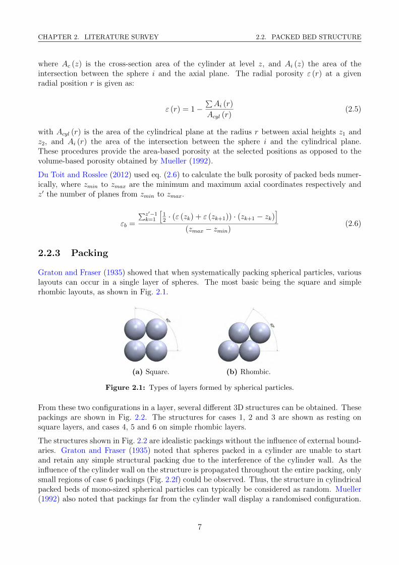
Graton and Fraser (1935) showed that when systematically packing spherical particles, variouslayouts can occur in a single layer of spheres. The most basic being the square and simplerhombic layouts, as shown in Fig. 2.1.
(a) Square. (b) Rhombic.
Figure 2.1: Types of layers formed by spherical particles.
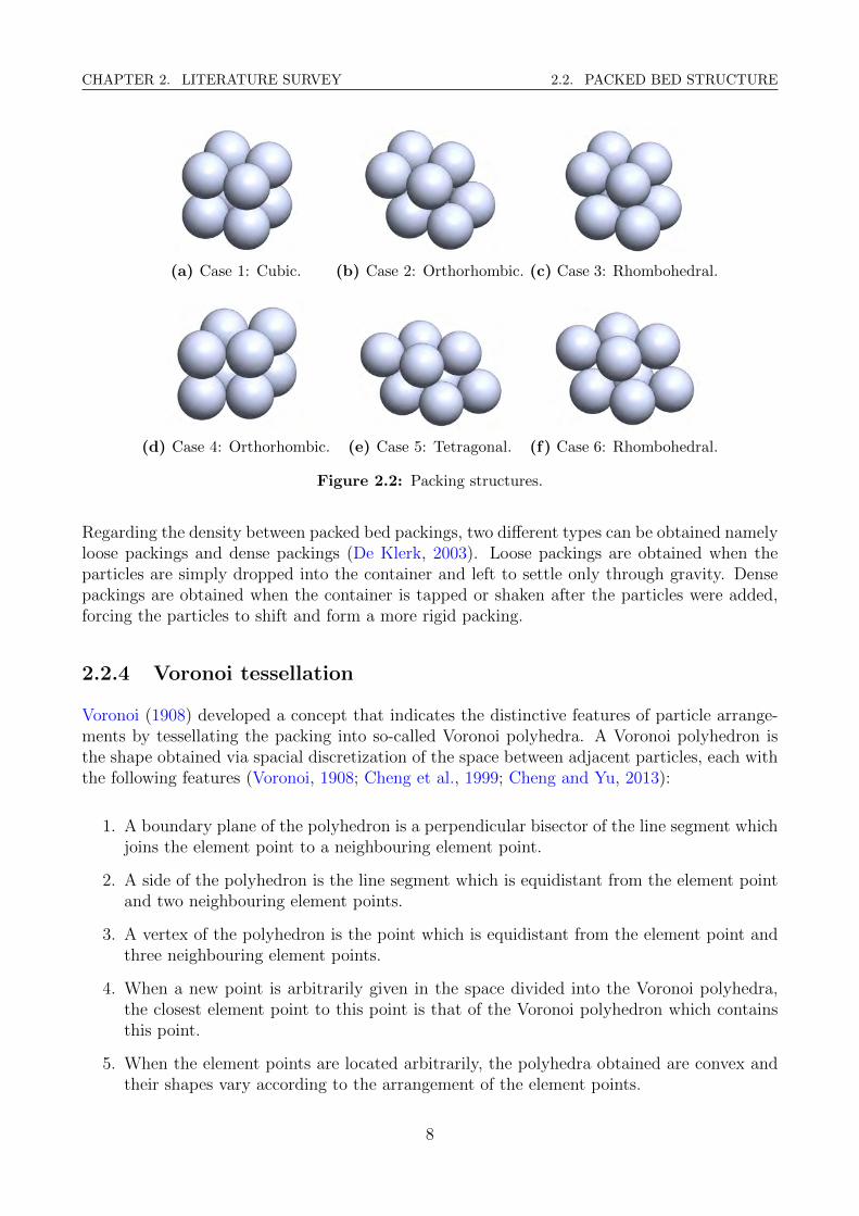
From these two configurations in a layer, several different 3D structures can be obtained. Thesepackings are shown in Fig. 2.2. The structures for cases 1, 2 and 3 are shown as resting onsquare layers, and cases 4, 5 and 6 on simple rhombic layers.
The structures shown in Fig. 2.2 are idealistic packings without the influence of external bound-aries. Graton and Fraser (1935) noted that spheres packed in a cylinder are unable to startand retain any simple structural packing due to the interference of the cylinder wall. As theinfluence of the cylinder wall on the structure is propagated throughout the entire packing, onlysmall regions of case 6 packings (Fig. 2.2f) could be observed. Thus, the structure in cylindricalpacked beds of mono-sized spherical particles can typically be considered as random. Mueller(1992) also noted that packings far from the cylinder wall display a randomised configuration.
7
CHAPTER 2. LITERATURE SURVEY 2.2. PACKED BED STRUCTURE
(a) Case 1: Cubic. (b) Case 2: Orthorhombic. (c) Case 3: Rhombohedral.
(d) Case 4: Orthorhombic. (e) Case 5: Tetragonal. (f) Case 6: Rhombohedral.
Figure 2.2: Packing structures.
Regarding the density between packed bed packings, two different types can be obtained namelyloose packings and dense packings (De Klerk, 2003). Loose packings are obtained when theparticles are simply dropped into the container and left to settle only through gravity. Densepackings are obtained when the container is tapped or shaken after the particles were added,forcing the particles to shift and form a more rigid packing.
2.2.4 Voronoi tessellation
Voronoi (1908) developed a concept that indicates the distinctive features of particle arrange-ments by tessellating the packing into so-called Voronoi polyhedra. A Voronoi polyhedron isthe shape obtained via spacial discretization of the space between adjacent particles, each withthe following features (Voronoi, 1908; Cheng et al., 1999; Cheng and Yu, 2013):
1. A boundary plane of the polyhedron is a perpendicular bisector of the line segment whichjoins the element point to a neighbouring element point.
2. A side of the polyhedron is the line segment which is equidistant from the element pointand two neighbouring element points.
3. A vertex of the polyhedron is the point which is equidistant from the element point andthree neighbouring element points.
4. When a new point is arbitrarily given in the space divided into the Voronoi polyhedra,the closest element point to this point is that of the Voronoi polyhedron which containsthis point.
5. When the element points are located arbitrarily, the polyhedra obtained are convex andtheir shapes vary according to the arrangement of the element points.
8
CHAPTER 2. LITERATURE SURVEY 2.2. PACKED BED STRUCTURE
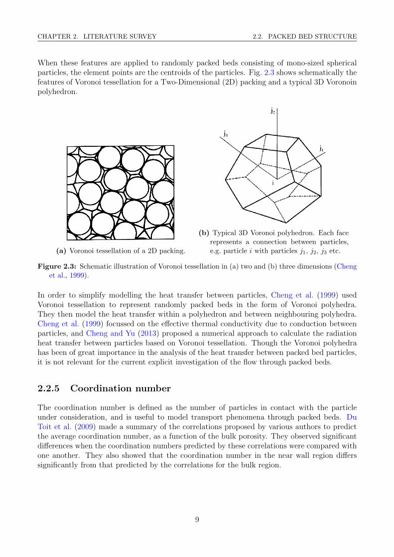
When these features are applied to randomly packed beds consisting of mono-sized sphericalparticles, the element points are the centroids of the particles. Fig. 2.3 shows schematically thefeatures of Voronoi tessellation for a Two-Dimensional (2D) packing and a typical 3D Voronoinpolyhedron.
(a) Voronoi tessellation of a 2D packing.
(b) Typical 3D Voronoi polyhedron. Each facerepresents a connection between particles,e.g. particle i with particles j1, j2, j3 etc.
Figure 2.3: Schematic illustration of Voronoi tessellation in (a) two and (b) three dimensions (Chenget al., 1999).
In order to simplify modelling the heat transfer between particles, Cheng et al. (1999) usedVoronoi tessellation to represent randomly packed beds in the form of Voronoi polyhedra.They then model the heat transfer within a polyhedron and between neighbouring polyhedra.Cheng et al. (1999) focussed on the effective thermal conductivity due to conduction betweenparticles, and Cheng and Yu (2013) proposed a numerical approach to calculate the radiationheat transfer between particles based on Voronoi tessellation. Though the Voronoi polyhedrahas been of great importance in the analysis of the heat transfer between packed bed particles,it is not relevant for the current explicit investigation of the flow through packed beds.
2.2.5 Coordination number
The coordination number is defined as the number of particles in contact with the particleunder consideration, and is useful to model transport phenomena through packed beds. DuToit et al. (2009) made a summary of the correlations proposed by various authors to predictthe average coordination number, as a function of the bulk porosity. They observed significantdifferences when the coordination numbers predicted by these correlations were compared withone another. They also showed that the coordination number in the near wall region differssignificantly from that predicted by the correlations for the bulk region.
9

CHAPTER 2. LITERATURE SURVEY 2.3. POROSITY VARIATIONS
2.2.6 Contact angles between adjacent particles
Du Toit et al. (2009) also defined a contact angle between two particles in contact with eachother as the angle between the line connecting the particle centroids, and the line perpendicularto the direction of the heat flux. Thus, a contact angle of 0◦ implies that the heat transferbetween two particles in contact does not contribute to the heat flux in the relevant coordinatesystem, and on the other hand a contact angle of 90◦ implies maximum contribution to theheat flux. Though using contact angles holds potential in simulating the effective thermalconductivity between adjacent particles, it is not of great relevance for the current investigation.
2.3 Porosity variations
As mentioned in Section 2.1, the design of a packed bed is based on the pressure drop of thefluid through the bed as well as mechanisms of heat and mass transfer. These mechanismsare all influenced by the bed porosity (Du Toit, 2008). For flow through a porous medium thepermeability increases with the porosity (White and Tien, 1987).
2.3.1 Porosity variations in the radial direction
Radial porosity variations is a geometrical characteristic of packed beds and is particularlyprominent at aspect ratios of α ≤ 10 (Mueller, 1997; De Klerk, 2003). These variations oc-cur because of the influence of the cylinder walls, see Section 2.3.2. Radial porosity varia-tions for cylindrical packed beds with mono-sized spheres have been investigated using variousexperimental and systematic methods (Mueller, 2010). Most of these investigations assumeaxi-symmetry and average the porosity tangentially.
Experimental investigations
Roblee et al. (1958) performed the first experiments to investigate the variation of porosity inthe radial direction in randomly packed beds. This was achieved by packing cork spheres into acardboard cylinder which was then filled with paraffin wax. After solidification, slabs were cutfrom the bed and each slab cut into annular rings. These annular rings were used to determinethe fraction of voids (wax). The cylinder wall had a definite influence on the porosity of thebed. Oscillatory variations of the porosity was observed further than 2 particle diameters intothe bed, the amplitude decreasing with increasing distance from the wall.
Benenati and Brosilow (1962) made packed beds by filling cylindrical containers with lead shot.The bed voids were then filled with epoxy resin and left to cure. The solid cylinder was thenmachined in stages to successively smaller diameters and the weight loss noted. They foundthat the porosity distribution took the form of a damped oscillatory wave with a maximum of1.0 at the wall and the oscillations damped out at roughly 4 to 5 particle diameters from thewall.
Ridgway and Tarbuck (1966) followed a technique whereby a cylinder with balls was revolved atspeeds of over 1000 rpm. Measuring the thickness of an annular layer of water, whilst gradually
10

CHAPTER 2. LITERATURE SURVEY 2.3. POROSITY VARIATIONS
adding water, the radial porosity distribution was calculated. Their results were similar tothat of Benenati and Brosilow (1962), with the porosity showing damped oscillatory behaviourwithin 5 particle diameters from the wall.
Goodling et al. (1983) made packed beds by filling a cylindrical plastic pipe with polystyrenespheres and then filling the voids with a mixture of epoxy and finely ground iron particles.After hardening, thin annular rings were cut from the bed perimeter over the whole length ona lathe. Noting the weight loss after each cut. They also found the porosity to show dampedoscillatory behaviour within 5 particle diameters of the wall.
Sederman et al. (2001) used magnetic resonance imaging volume-visualisation in combinationwith image analysis techniques to analyse the porosity distribution in cylindrical packed bedsfilled with ballotini spheres. Their results were similar to that of Goodling et al. (1983).
The porosity variations in the near wall region of cylindrical packed beds have been experi-mentally investigated by numerous researchers. De Klerk (2003) compiled the radial porositydistributions obtained by some of the researchers mentioned above, see Fig. 2.4. He concludedthat, even though the experimental work was approached in different ways, the results were ingeneral agreement.
Figure 2.4: Radial porosity variation, De Klerk (2003).
Modelling of porosity variations
Various attempts at modelling the near-wall porosity variations have been presented in liter-ature. These efforts to predict the porosity vary from entirely empirical in nature to semi-analytical predictive expressions (Mueller, 2012). Most of the recent models succeed in de-scribing both the oscillatory and damping characteristics of the porosity variations (De Klerk,2003).
11

CHAPTER 2. LITERATURE SURVEY 2.3. POROSITY VARIATIONS
Van Antwerpen et al. (2010) gives a summary of relevant correlations to determine the oscilla-tory porosity variations in cylindrical packed beds. They also concluded that there is a tendencyto move away from purely empirical correlations to the analysis of numerically simulated packedbeds. However, what is of importance is that methods do exist which make it possible to ob-tain the radial porosity variations in a cylindrical packed bed of spherical particles, when thecoordinates of the centres of the spheres are known.
2.3.2 Effect of cylinder wall on porosity
As mentioned in Section 2.3.1, Benenati and Brosilow (1962) performed an experimental studyto obtain the radial porosity distribution in packed beds. They found that the porosity dis-tribution took the form of a damped oscillatory wave which damped out at roughly 5 particlediameters from the wall. They also investigated the porosity variations in the radial direction inlarge packed beds containing a central steel rod. They observed the same oscillatory behaviourof the porosity regardless of whether it was the inner surface (steel rod) or the outer surface(cylinder wall). This showed that the presence of any distinct boundary or wall causes theobserved oscillatory porosity variations.
Mariani et al. (2009) used Computed Tomography (CT) techniques to obtain the particle centredistribution for a packed bed with an aspect ratio of α = 5.04. They found that the first layerof particles adjacent to the wall was highly ordered, with almost all of the particle centres beingat a distance of a particle radius from the wall. The second layer showed a definite disorder inthe distribution of the particle centres in the radial direction. This development of decreasingorder in the positions of the particle centres from the cylinder wall continues toward the centreof the bed.
Mueller (2010) presented a particle centre distribution for a packed bed with an aspect ratio ofα = 7.99. His findings was similar to that of Mariani et al. (2009), as shown in Fig. 2.5.
Figure 2.5: Distribution of the centre coordinates of the spheres of a bed with α = 7.99, Mueller(2010).
Wensrich (2012) also used CT scans of packed beds with various aspect ratios to examine theeffect of the cylinder boundaries on the packing structure. As with previous studies, they found
12

CHAPTER 2. LITERATURE SURVEY 2.3. POROSITY VARIATIONS
the particles against the wall to have a great deal of order. This is because the wall, whichis two-dimensional in nature, forces a two-dimensional ordered structure in the first layer ofparticles.
2.3.3 Porosity variations in the axial direction
As mentioned in Section 2.3.2, the presence of any distinct boundary or wall in a packed bedcauses oscillatory porosity variations near the wall due to the ordered structure of the packingof the near wall particles. This is also true for the top/bottom walls of the bed.
Zou and Yu (1995) described the influence on the porosity variations in a cylindrical packedbed, due to the top/bottom walls as well as the length of the bed, as the length effect. Theyobserved that most investigations on porosity variations in packed beds considered only theside wall effect, whilst implicitly assuming the length effect to be negligible. They also statedthat the error due to this assumption is usually small, but must be considered when the lengthof the bed is small compared to its diameter. Zou and Yu (1995) studied the influence of thebed length to particle diameter ratio (L/d) on the bulk porosity by considering a packed bedwith an aspect ratio of α = 24.66. They found that for L/d ≤ 20 the bulk porosity increasedfrom εb = 0.395 to εb = 0.46 at L/d = 2.5.
2.3.4 Porosity variations as a function of the aspect ratio
Leva and Grummer (1947) made packed beds using a steel pipe and glass spheres. Knowing thenumber of particles in the bed, particle diameter, packing height and cylinder diameter theycalculated the bed average porosity. Using this method they measured the average porosity ofnumerous beds with different aspect ratios, for loose and dense packings.
De Klerk (2003) performed similar experiments as Leva and Grummer (1947), with loose pack-ings. Fig. 2.6 shows that they observed similar results. It is clear that the average bed porosityincreases for α ≤ 12.
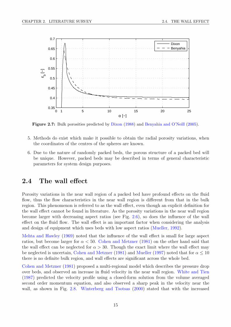
Dixon (1988) made packed beds with aspect ratios of 1 ≤ α ≤ 10, and measured the bulkporosity of each bed using a weighing method. He repeated the experiment for each aspectratio with two different cylinder lengths, in order to eliminate the length effect. Using his ownmeasurements, as well as data from literature, he derived correlations which predict the bulkporosity of packed beds, as a function of the reciprocal of the aspect ratio. The correlation byDixon (1988) which predicts the bulk porosity is shown in eq. (2.7), where d/D is the reciprocalof α. Fig. 2.7 shows a plot of the bulk porosities predicted by eq. (2.7).
εb =
0.4 + 0.05 (d/D) + 0.412 (d/D)2 for d/D ≤ 0.5
0.528 + 2.464 ((d/D)− 0.5) for 0.5 ≤ d/D ≤ 0.536
1− 0.667 (d/D)3 (2 (d/D)− 1)−0.5 for 0.536 ≤ d/D
(2.7)
Benyahia and O’Neill (2005) measured the bulk porosities of packed beds with aspect ratiosof 1.5 ≤ α ≤ 50, using a water displacement method. Using their measurements, they also
13

CHAPTER 2. LITERATURE SURVEY 2.3. POROSITY VARIATIONS
Figure 2.6: Average bed porosity as a function of the aspect ratio, De Klerk (2003).
developed a correlation, eq. (2.8), which predicts the bulk porosity of packed beds, as a functionof the aspect ratio.
εb = 0.39 +1.74
(α + 1.14)2 (2.8)
Fig. 2.7 shows the bulk porosities predicted by eqns. (2.7) and (2.8), by Dixon (1988) andBenyahia and O’Neill (2005) respectively. It should be noted that both Dixon (1988) andBenyahia and O’Neill (2005) used packed beds long enough to eliminate the length effect.
2.3.5 Conclusions on porosity
Considering the literature mentioned in this section, the following important conclusions canbe made regarding the porosity variations in cylindrical packed beds consisting of mono-sizedspherical particles:
1. Particles in the near wall region have an ordered packing due to the two-dimensionalityof the wall.
2. The porosity varies in an oscillatory fashion in the near-wall region.
3. The amplitude of the oscillations are increasingly damped out as the distance from thewall increases.
4. The presence of any distinct boundary or wall causes the above mentioned oscillatoryporosity variations.
14
CHAPTER 2. LITERATURE SURVEY 2.4. THE WALL EFFECT
0 1 5 10 15 20 250.35
0.4
0.45
0.5
0.55
0.6
0.65
0.7ε b [−
]
α [−]
DixonBenyahia
Figure 2.7: Bulk porosities predicted by Dixon (1988) and Benyahia and O’Neill (2005).
5. Methods do exist which make it possible to obtain the radial porosity variations, whenthe coordinates of the centres of the spheres are known.
6. Due to the nature of randomly packed beds, the porous structure of a packed bed willbe unique. However, packed beds may be described in terms of general characteristicparameters for system design purposes.
2.4 The wall effect
Porosity variations in the near wall region of a packed bed have profound effects on the fluidflow, thus the flow characteristics in the near wall region is different from that in the bulkregion. This phenomenon is referred to as the wall effect, even though an explicit definition forthe wall effect cannot be found in literature. As the porosity variations in the near wall regionbecome larger with decreasing aspect ratios (see Fig. 2.6), so does the influence of the walleffect on the fluid flow. The wall effect is an important factor when considering the analysisand design of equipment which uses beds with low aspect ratios (Mueller, 1992).
Mehta and Hawley (1969) noted that the influence of the wall effect is small for large aspectratios, but become larger for α < 50. Cohen and Metzner (1981) on the other hand said thatthe wall effect can be neglected for α > 30. Though the exact limit where the wall effect maybe neglected is uncertain, Cohen and Metzner (1981) and Mueller (1997) noted that for α ≤ 10there is no definite bulk region, and wall effects are significant across the whole bed.
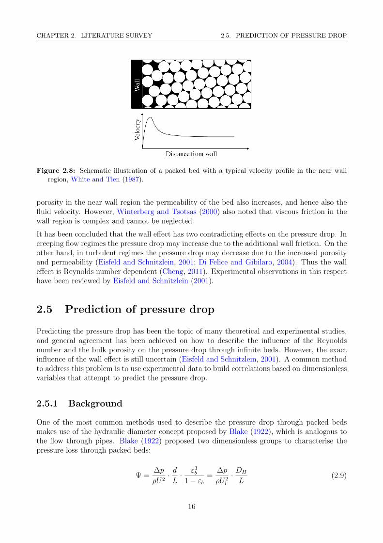
Cohen and Metzner (1981) proposed a multi-regional model which describes the pressure dropover beds, and observed an increase in fluid velocity in the near wall region. White and Tien(1987) predicted the velocity profile using a closed-form solution from the volume averagedsecond order momentum equation, and also observed a sharp peak in the velocity near thewall, as shown in Fig. 2.8. Winterberg and Tsotsas (2000) stated that with the increased
15
CHAPTER 2. LITERATURE SURVEY 2.5. PREDICTION OF PRESSURE DROP
Figure 2.8: Schematic illustration of a packed bed with a typical velocity profile in the near wallregion, White and Tien (1987).
porosity in the near wall region the permeability of the bed also increases, and hence also thefluid velocity. However, Winterberg and Tsotsas (2000) also noted that viscous friction in thewall region is complex and cannot be neglected.
It has been concluded that the wall effect has two contradicting effects on the pressure drop. Increeping flow regimes the pressure drop may increase due to the additional wall friction. On theother hand, in turbulent regimes the pressure drop may decrease due to the increased porosityand permeability (Eisfeld and Schnitzlein, 2001; Di Felice and Gibilaro, 2004). Thus the walleffect is Reynolds number dependent (Cheng, 2011). Experimental observations in this respecthave been reviewed by Eisfeld and Schnitzlein (2001).
2.5 Prediction of pressure drop
Predicting the pressure drop has been the topic of many theoretical and experimental studies,and general agreement has been achieved on how to describe the influence of the Reynoldsnumber and the bulk porosity on the pressure drop through infinite beds. However, the exactinfluence of the wall effect is still uncertain (Eisfeld and Schnitzlein, 2001). A common methodto address this problem is to use experimental data to build correlations based on dimensionlessvariables that attempt to predict the pressure drop.
2.5.1 Background
One of the most common methods used to describe the pressure drop through packed bedsmakes use of the hydraulic diameter concept proposed by Blake (1922), which is analogous tothe flow through pipes. Blake (1922) proposed two dimensionless groups to characterise thepressure loss through packed beds:
Ψ =∆p
ρU2· dL· ε3
b
1− εb=
∆p
ρU2i
· DH
L(2.9)
16
CHAPTER 2. LITERATURE SURVEY 2.5. PREDICTION OF PRESSURE DROP
Rem =Rep
1− ε; Rep =
ρUd
µ(2.10)
with Ui the interstitial velocity, U the superficial velocity, DH the hydraulic diameter, Repthe particle Reynolds number, ρ the fluid density and µ the fluid dynamic viscosity. The twogroups, Ψ and Rem, are known as the modified friction factor and the modified Reynolds numberrespectively. However, the hydraulic diameter concept suggested by Blake (1922) was derivedfor infinite beds, and excluded the effect of the wall on the hydraulic diameter. Also, Ergun(1952) stated that these early attempts to describe the pressure drop through packed bedsfailed, because they did not consider the fact that the pressure drop is caused by simultaneouskinetic and viscous effects.
2.5.2 Types of equations
Reynolds (1900) was the first to correlate the resistance offered by friction to the motion of thefluid as the sum of the viscous and kinetic energy losses:
∆p
L= aµU + bρUn (2.11)
with the term aµU representing viscous energy losses, bρUn kinetic energy losses, and n = 2.Various authors have found the viscous energy loss to be proportional to (1− εb)2/ε3
b and thekinetic energy loss to (1− εb)/ε3
b . Ergun (1952) expressed these proportionalities as:
a = a′ · (1− εb)2
ε3b
; b = b′ · (1− εb)ε3b
(2.12)
where values for a′ and b′ were obtained empirically. Substituting eq. (2.12) into eq. (2.11), andrewriting in terms of the friction factor for the general case yields:
Ψ =∆p
ρU2· dL· ε3
b
1− εb=
a′
Rem+
b′
(Rem)2−n (2.13)
Eq. (2.13) is the most general form of the friction factor for fluid flow through packed beds,based on the hydraulic diameter concept. Two main variations exist on this general form:
1. Ergun-type equations.Ergun-type equations are variations of eq. (2.13) for which n = 2, as originally proposedby Reynolds (1900). These equations are arguably the most widely used correlations topredict the pressure drop through packed beds.
2. Carman-type equations.Carman-type equations are variations of eq. (2.13) for which 1.9 ≤ n ≤ 1.95, as proposedby Carman (1937).
17
CHAPTER 2. LITERATURE SURVEY 2.5. PREDICTION OF PRESSURE DROP
Known as the Ergun equation, Ergun (1952) originally obtained values for the constants asa′ = 150 and b′ = 1.75, by fitting eq. (2.13) to 640 experimental data points. These data pointsincluded pressure drop measurements for the flow through beds packed with particles of variousshapes and sizes, such as various sized spheres, sand and pulverized coke. The Ergun equationis valid within the ranges of 1 < Rep < 2500 and 0.36 ≤ εb ≤ 0.4.
The Ergun equation, however, assumes the influence of the containing walls to be negligible anddoes not take the wall effect into account. As a result, many researchers have fitted eq. (2.13)to their own experimental data for beds with different aspect ratios, attempting to include thewall effect in the empirically determined constants a′ and b′. Therefore, a large number of thesecorrelations exist, of which only a few are relevant for the current investigation.
Carman (1937) originally obtained values for the constants as a′ = 180 and b′ = 2.871, which isknown as the Carman equation. Even though a number of variations of Carman-type equationsdo exist, they are less known and have not received as much attention or credit as Ergun-typeequations.
2.5.3 The KTA correlation
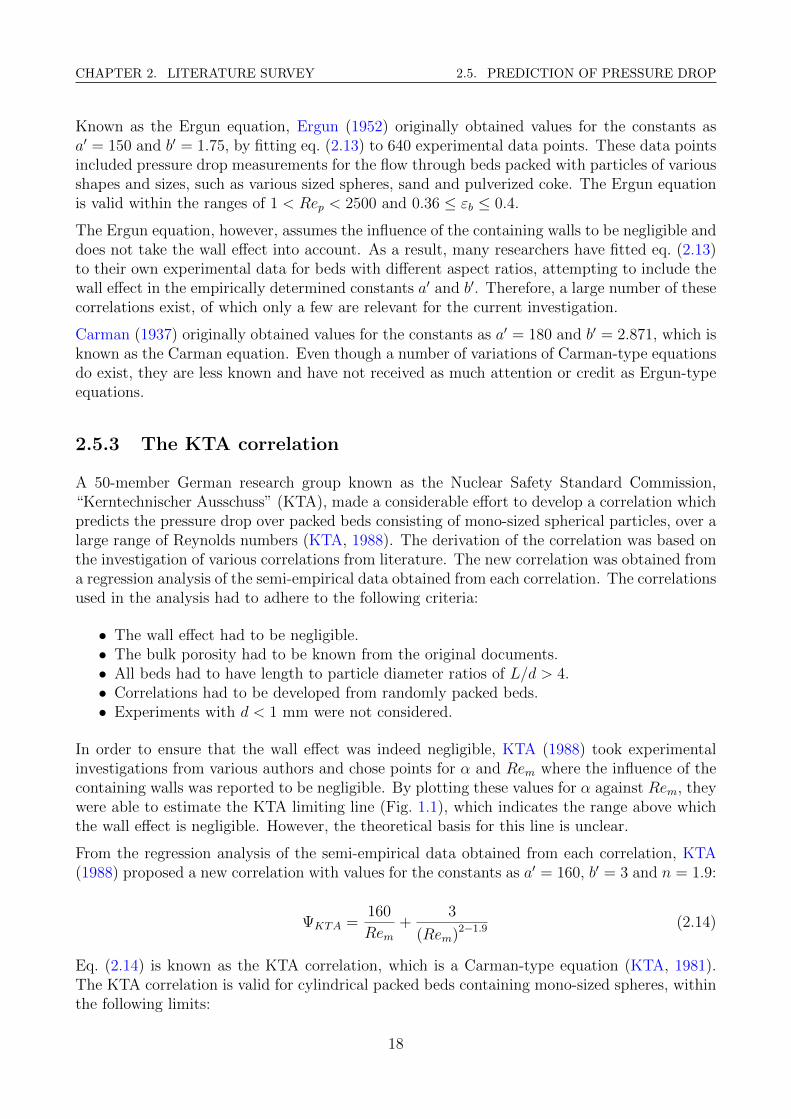
A 50-member German research group known as the Nuclear Safety Standard Commission,“Kerntechnischer Ausschuss” (KTA), made a considerable effort to develop a correlation whichpredicts the pressure drop over packed beds consisting of mono-sized spherical particles, over alarge range of Reynolds numbers (KTA, 1988). The derivation of the correlation was based onthe investigation of various correlations from literature. The new correlation was obtained froma regression analysis of the semi-empirical data obtained from each correlation. The correlationsused in the analysis had to adhere to the following criteria:
• The wall effect had to be negligible.• The bulk porosity had to be known from the original documents.• All beds had to have length to particle diameter ratios of L/d > 4.• Correlations had to be developed from randomly packed beds.• Experiments with d < 1 mm were not considered.
In order to ensure that the wall effect was indeed negligible, KTA (1988) took experimentalinvestigations from various authors and chose points for α and Rem where the influence of thecontaining walls was reported to be negligible. By plotting these values for α against Rem, theywere able to estimate the KTA limiting line (Fig. 1.1), which indicates the range above whichthe wall effect is negligible. However, the theoretical basis for this line is unclear.
From the regression analysis of the semi-empirical data obtained from each correlation, KTA(1988) proposed a new correlation with values for the constants as a′ = 160, b′ = 3 and n = 1.9:
ΨKTA =160
Rem+
3
(Rem)2−1.9 (2.14)
Eq. (2.14) is known as the KTA correlation, which is a Carman-type equation (KTA, 1981).The KTA correlation is valid for cylindrical packed beds containing mono-sized spheres, withinthe following limits:
18
CHAPTER 2. LITERATURE SURVEY 2.5. PREDICTION OF PRESSURE DROP
• Reynolds number: 100 < Rem < 105.• Porosity: 0.36 < ε < 0.42.• Bed length: L > 5d.• Aspect ratios above the limiting line in accordance with Fig. 1.1.
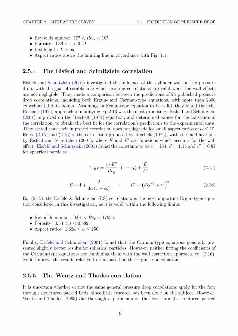
2.5.4 The Eisfeld and Schnitzlein correlation
Eisfeld and Schnitzlein (2001) investigated the influence of the cylinder wall on the pressuredrop, with the goal of establishing which existing correlations are valid when the wall effectsare not negligible. They made a comparison between the predictions of 24 published pressuredrop correlations, including both Ergun- and Carman-type equations, with more than 2300experimental data points. Assuming an Ergun-type equation to be valid, they found that theReichelt (1972) approach of modifying eq. 2.13 was the most promising. Eisfeld and Schnitzlein(2001) improved on the Reichelt (1972) equation, and determined values for the constants inthe correlation, to obtain the best fit for the correlation’s predictions to the experimental data.They stated that their improved correlation does not degrade for small aspect ratios of α ≤ 10.Eqns. (2.15) and (2.16) is the correlation proposed by Reichelt (1972), with the modificationsby Eisfeld and Schnitzlein (2001), where E and E ′ are functions which account for the walleffect. Eisfeld and Schnitzlein (2001) found the constants to be e = 154, e′ = 1.15 and e′′ = 0.87for spherical particles.
ΨES =e · E2
Rep· (1− εb) +
E
E ′(2.15)
E = 1 +2
3α (1− εb); E ′ =
(e′α−2 + e′′
)2(2.16)
Eq. (2.15), the Eisfeld & Schnitzlein (ES) correlation, is the most important Ergun-type equa-tion considered in this investigation, as it is valid within the following limits:
• Reynolds number: 0.01 < Rep < 17635.• Porosity: 0.33 < ε < 0.882.• Aspect ratios: 1.624 ≤ α ≤ 250.
Finally, Eisfeld and Schnitzlein (2001) found that the Carman-type equations generally pre-sented slightly better results for spherical particles. However, neither fitting the coefficients ofthe Carman-type equations nor combining them with the wall correction approach, eq. (2.16),could improve the results relative to that based on the Ergun-type equation.
2.5.5 The Wentz and Thodos correlation
It is uncertain whether or not the same general pressure drop correlations apply for the flowthrough structured packed beds, since little research has been done on the subject. However,Wentz and Thodos (1963) did thorough experiments on the flow through structured packed
19
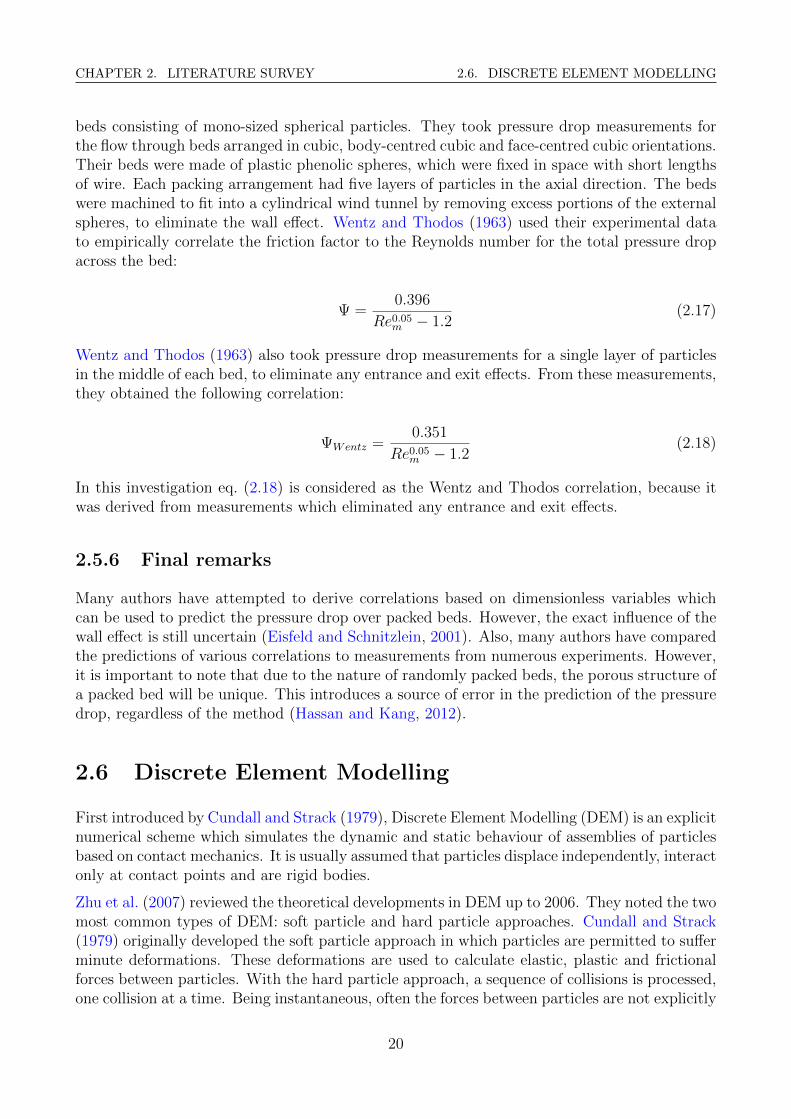
CHAPTER 2. LITERATURE SURVEY 2.6. DISCRETE ELEMENT MODELLING
beds consisting of mono-sized spherical particles. They took pressure drop measurements forthe flow through beds arranged in cubic, body-centred cubic and face-centred cubic orientations.Their beds were made of plastic phenolic spheres, which were fixed in space with short lengthsof wire. Each packing arrangement had five layers of particles in the axial direction. The bedswere machined to fit into a cylindrical wind tunnel by removing excess portions of the externalspheres, to eliminate the wall effect. Wentz and Thodos (1963) used their experimental datato empirically correlate the friction factor to the Reynolds number for the total pressure dropacross the bed:
Ψ =0.396
Re0.05m − 1.2
(2.17)
Wentz and Thodos (1963) also took pressure drop measurements for a single layer of particlesin the middle of each bed, to eliminate any entrance and exit effects. From these measurements,they obtained the following correlation:
ΨWentz =0.351
Re0.05m − 1.2
(2.18)
In this investigation eq. (2.18) is considered as the Wentz and Thodos correlation, because itwas derived from measurements which eliminated any entrance and exit effects.
2.5.6 Final remarks
Many authors have attempted to derive correlations based on dimensionless variables whichcan be used to predict the pressure drop over packed beds. However, the exact influence of thewall effect is still uncertain (Eisfeld and Schnitzlein, 2001). Also, many authors have comparedthe predictions of various correlations to measurements from numerous experiments. However,it is important to note that due to the nature of randomly packed beds, the porous structure ofa packed bed will be unique. This introduces a source of error in the prediction of the pressuredrop, regardless of the method (Hassan and Kang, 2012).
2.6 Discrete Element Modelling
First introduced by Cundall and Strack (1979), Discrete Element Modelling (DEM) is an explicitnumerical scheme which simulates the dynamic and static behaviour of assemblies of particlesbased on contact mechanics. It is usually assumed that particles displace independently, interactonly at contact points and are rigid bodies.
Zhu et al. (2007) reviewed the theoretical developments in DEM up to 2006. They noted the twomost common types of DEM: soft particle and hard particle approaches. Cundall and Strack(1979) originally developed the soft particle approach in which particles are permitted to sufferminute deformations. These deformations are used to calculate elastic, plastic and frictionalforces between particles. With the hard particle approach, a sequence of collisions is processed,one collision at a time. Being instantaneous, often the forces between particles are not explicitly
20
CHAPTER 2. LITERATURE SURVEY 2.7. COMPUTATIONAL FLUID DYNAMICS
considered. Zhu et al. (2007) also noted that DEM, particularly the soft particle approach, hasbeen extensively used to study various phenomena, such as particle packing, heaping and pilingprocesses, hopper flow and mixing. They also stated that the models for calculating the contactforces between particles have improved and that more forces have been implemented, whichmakes DEM more applicable to particulate research. For more information, Section 3.1 gives atheoretical background of DEM as employed in STAR-CCM+ R©.
With regards to DEM used in studying packed beds, Eppinger et al. (2011) generated randomlypacked beds by initialising spherical particles within a cylindrical domain, which dropped tothe bottom of the tube due to gravity. For each particle a force balance was solved whichtook into account the forces of gravity, interaction between particles and interaction betweenparticles and the cylinder wall. They found good agreement for global bed porosity and radialporosity distributions between their DEM results and results found in literature. Theron (2011)investigated the capability of STAR-CCM+ R© to perform DEM simulations. He generatedrandomly packed beds with aspect ratios of 1.39 ≤ α ≤ 4.93, using a similar method asEppinger et al. (2011), and validated the results using experimental data. The DEM resultscompared well with the experimental data and showed similar trends for porosity variations inthe axial direction. Theron (2011) concluded that DEM is an appropriate tool for simulatingpacked bed arrangements.
2.7 Computational Fluid Dynamics
Computational Fluid Dynamics (CFD) is the analysis of systems involving fluid flow, heattransfer and associated phenomena such as chemical reactions by means of computer basedsimulations (Versteeg and Malalasekera, 2007). CFD allows for the explicit simulation of fluidflow between packed bed particles, taking each particle’s position and geometric properties intoaccount. With the tremendous increase in computational power, and the parallel developmentof various numerical techniques, CFD has become a viable method to analyse the complex flowsin packed beds (Eppinger et al., 2011; Reddy and Joshi, 2010).
2.7.1 CFD and packed beds
Calis et al. (2001) used a commercial CFD package to simulate the flow through structuredpacked beds consisting of 16 particles and aspect ratios of 1 ≤ α ≤ 2. The local velocity profileon a cross section of the bed, predicted by the CFD simulation, agreed well with the profilemeasured in their experimental study. They concluded that CFD is a viable method to predictthe pressure drop over packed beds, with an average error of about 10%.
Hassan (2008) simulated the flow between spherical particles with a rhombohedral packing (Fig.2.2c). Hassan (2008) stated that most previous experimental studies were restricted to under-standing the global parameters, and that local information of the flow velocity and patternswere scarce. However, his study showed that with the new developments in computationaltechniques, it is now possible to gain detailed insight into the flow between bed particles.
Bai et al. (2009) performed experiments and CFD simulations for both structured and randompackings with up to 150 particles. Their predicted pressure drops matched well with the ex-
21
CHAPTER 2. LITERATURE SURVEY 2.7. COMPUTATIONAL FLUID DYNAMICS
perimental measurements, with errors less than 10%. They also noticed a discrepancy betweenempirical correlations which predict the pressure drop at low aspect ratios, and their CFDpredictions.
Reddy and Joshi (2010) described the deviations between the pressure drop predicted by theErgun equation and experimental results at low aspect ratios, by simulating the flow throughrandomly packed beds with aspect ratios of α = 3, 5 and 10 at 0.1 < Rep < 10000. Their CFDresults showed an increase in pressure drop at low Reynolds numbers, and a decrease at highReynolds numbers, thus giving evidence to the wall effect.
Eppinger et al. (2011) used STAR-CCM+ R© to investigate the flow patterns in randomly packedbeds with aspect ratios of 3 ≤ α ≤ 10 in laminar, transition and turbulent regimes. Theycompared their CFD results for porosity and pressure drop with results from literature, andconfirmed that physically correct results for flow characteristics in packed beds can be obtainedusing CFD. Theron (2011) performed a similar investigation and also found good agreementbetween his CFD results and that found in literature.
CFD investigations on the flow between packed bed particles have increased drastically in recentyears due to the increase of computational power and the development of numerical techniques.Many authors have found good agreement between their own CFD predictions, experimentalmeasurements and results from literature. However, some key issues with regards to modellingthe flow through these complex geometries still exist, such as (1) mesh generation, (2) contacttreatment and (3) turbulence solvers (Theron, 2011).
2.7.2 Meshing packed beds
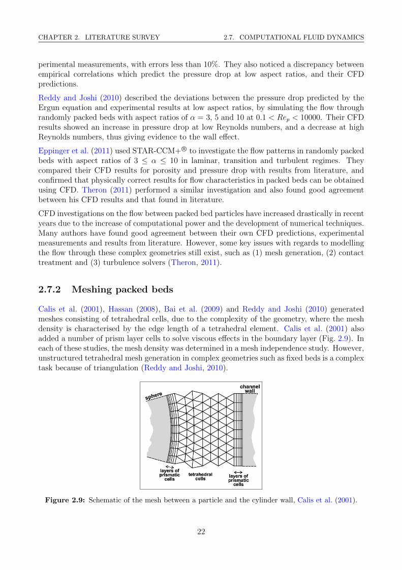
Calis et al. (2001), Hassan (2008), Bai et al. (2009) and Reddy and Joshi (2010) generatedmeshes consisting of tetrahedral cells, due to the complexity of the geometry, where the meshdensity is characterised by the edge length of a tetrahedral element. Calis et al. (2001) alsoadded a number of prism layer cells to solve viscous effects in the boundary layer (Fig. 2.9). Ineach of these studies, the mesh density was determined in a mesh independence study. However,unstructured tetrahedral mesh generation in complex geometries such as fixed beds is a complextask because of triangulation (Reddy and Joshi, 2010).
Figure 2.9: Schematic of the mesh between a particle and the cylinder wall, Calis et al. (2001).
22
CHAPTER 2. LITERATURE SURVEY 2.7. COMPUTATIONAL FLUID DYNAMICS
Eppinger et al. (2011) and Preller (2011) used polyhedral and thin volume meshes respectively.Both investigated the influence of the number of prism layers used, and found that 2 prismlayers offer the highest quality cells, without an excessive cell count.
Though the number of CFD investigations on the flow between packed bed particles haveincreased in recent years, the best practice for cell type and mesh density has not yet been es-tablished conclusively. However, with the ongoing expansion of meshing techniques, performinga mesh independence study is an integral part of any CFD investigation.
2.7.3 Contact treatment
A crucial point for the mesh generation in packed beds is the cell quality near the contact pointsbetween particles, and between particles and the cylinder wall. Due to its geometric nature, thecontact points force the flow area around it to be very small, thin and acute. The cells near thecontact points are usually either highly skewed or highly refined. High numbers of skewed cellslead to convergence problems during the calculation, whereas highly refined regions increasethe number of cells and as a direct consequence the computational time (Eppinger et al., 2011).Several methods to overcome this problem has been presented in literature.
Calis et al. (2001), Reddy and Joshi (2008) and Reddy and Joshi (2010) eliminated contactpoints entirely by reducing their particle diameters by 1.0% without changing the particlepositions, thus creating a gap between particles which improves the generated mesh. Bai et al.(2009) followed the same principle by reducing their particle diameter by 0.5%. Reddy andJoshi (2008) showed that the fluid velocity in the gap between the spheres is practically zero,and concluded that the gap does not affect the flow pattern. However, the particle shrinkagedirectly affects the packing porosity and therefore also the pressure drop. Since the pressuredrop is known to be very sensitive to the bed porosity, these authors needed correction factorsfor porosity and pressure drop to be able to compare their CFD results with the predictedvalues from correlations.
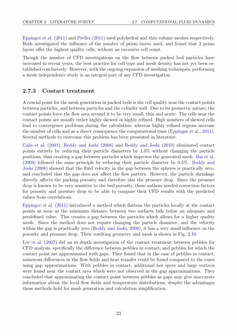
Eppinger et al. (2011) introduced a method which flattens the particles locally at the contactpoints as soon as the minimum distance between two surfaces falls below an adequate andpredefined value. This creates a gap between the particles which allows for a higher qualitymesh. Since the method does not require changing the particle diameter, and the velocitywithin the gap is practically zero (Reddy and Joshi, 2008), it has a very small influence on theporosity and pressure drop. Their resulting geometry and mesh is shown in Fig. 2.10.
Lee et al. (2007) did an in depth investigation of the contact treatment between pebbles forCFD analysis, specifically the difference between pebbles in contact, and pebbles for which thecontact point are approximated with gaps. They found that in the case of pebbles in contact,numerous differences in the flow fields and heat transfer could be found compared to the casesusing gap approximations. With pebbles in contact, additional hot spots and large vorticeswere found near the contact area which were not observed in the gap approximations. Theyconcluded that approximating the contact point between pebbles as gaps may give inaccurateinformation about the local flow fields and temperature distributions, despite the advantagesthese methods hold for mesh generation and calculation simplification.
23
CHAPTER 2. LITERATURE SURVEY 2.7. COMPUTATIONAL FLUID DYNAMICS
Figure 2.10: Artificial gap between two spheres, Eppinger et al. (2011).
Reyneke (2009) approximated the contact between particles by connecting particles at thecontact point with a small cylindrical shape, thus removing the region near the contact pointfrom the fluid domain. His results showed that the macroscopic flow properties, such as pressuredrop, were not influenced by the cylinders. Reyneke (2009) did not investigate the method’sinfluence on porosity or temperature distribution.
Dixon et al. (2013) did an in depth investigation of the influence of four different contacttreatments on the flow through packed beds. They tested two global methods in which particleswere either enlarged or shrunk uniformly, and two local methods in which particles were locallyflattened, similar to Eppinger et al. (2011), and locally connected with bridges, similar toReyneke (2009). Dixon et al. (2013) investigated the influence of the different methods on dragcoefficients as well as heat transfer between particles. They found that global methods gavehigh errors in both drag coefficient and heat transfer rates between particles, unless the particleenlargements or shrinkages were very small, in which case the method does not solve the meshingproblems. They found good results for drag coefficients for local methods. However, the methodsuggested by Eppinger et al. (2011), which creates small gaps between particles, presentedunrealistic results for heat transfer between particles. Dixon et al. (2013) recommended a localbridging method with a suitably defined effective thermal conductivity for the bridge material.
Dixon et al. (2013) also noted that their recommendations were based solely on reducing effectsof contact point modifications on the fluid flow and heat transfer between particles, and didnot consider implementation. They also noted that their analysis does not replace the need formesh independence studies or validation of simulations against experimental data.
2.7.4 Turbulence models
In any CFD calculation, the selection of an appropriate turbulence model is of great importancein order to obtain accurate predictions and capture the details of the flow parameters. Manymethods exist to describe or solve turbulence effects, for which detailed descriptions can befound in Versteeg and Malalasekera (2007) or CD-Adapco (2012), however the three mainapproaches to modelling turbulence are:
1. Turbulence models for Reynolds-Average Navier-Stokes (RANS) equations.Prior to the application of the numerical methods the Navier-Stokes equations are time
24
CHAPTER 2. LITERATURE SURVEY 2.7. COMPUTATIONAL FLUID DYNAMICS
averaged. Thus turbulence is modelled by focussing on the effects of turbulence on meanflow properties. The computational resources required for reasonably accurate solutionsare modest. Common models used in the RANS approach are k− ε models, k−ω modelsand Reynolds Stress Models (RSM).
2. Large Eddy Simulation (LES).LES is an inherently transient technique which solves the behaviour of large 3D eddies,while the effects of small eddies on the flow are treated using sub-grid models. Explicitlysolving large scales of turbulence provides more accurate solutions compared to RANSmodels, but also requires more computational resources.
3. Direct Numerical Simulation (DNS).DNS computes all turbulent velocity fluctuations, and provides extremely detailed andaccurate solutions for turbulence. However, DNS demands extremely fine meshes and iseven more computationally intensive than LES.
Calis et al. (2001) investigated the difference between the RSM and k − ε models, and foundthat the more computationally intensive RSM model yielded only slightly better pressure dropresults. They considered the difference too small to justify the extra computational demand,and thus used the k − ε model.
Bai et al. (2009) examined different RANS turbulence models to understand their effects onthe accuracy of the pressure drop prediction. They simulated the flow over a single packed bed,while varying only the turbulence model, and compared the CFD predictions with their ownexperimental results. Bai et al. (2009) found no significant difference among various k − ε andk − ω models, with variations of pressure drop less than 4.0%. The RSM model’s predictedpressure drops were closest to the experimental measurements. However, it took 3 times longerto solve, while the k − ε model results were within 3.0% of the RSM model results. The extracomputation effort required by the RSM model was not justified, thus they used the k − εmodel.
Hassan (2008) used LES in his study of the flow within a segment of a pebble bed core, afterweighing the advantages and disadvantages of RANS, LES and DNS. Hassan (2008) statedthat LES is a compromise between DNS and RANS, as it is more accurate than RANS andless computationally intensive than DNS.
Preller (2011) did a comprehensive study to determine which turbulence models are appropriatefor flows in packed beds by comparing various factors from the Realisable k− ε, RSM and LESmodels. He found that the predicted pressure drops between these models varied less than 3.0%for a wide range of Reynolds numbers. He concluded then that more computationally intensivemodels, such as LES and RSM, offer little improvement in accuracy over the k − ε models.
2.7.5 Inlet boundary condition
For the sake of simplicity, Bai et al. (2009), Reddy and Joshi (2010) and Eppinger et al. (2011)all specified uniform velocity profiles at the inlet boundary. Fig. 2.11a shows such a profile,where U (r) is the velocity profile as a function of the cylinder radius, and Uavg the average
25

CHAPTER 2. LITERATURE SURVEY 2.7. COMPUTATIONAL FLUID DYNAMICS
velocity. However, a constant velocity profile is an ideal case where the flow is considered to beinviscid.
(a) Inviscid. (b) Laminar. (c) Turbulent.
Figure 2.11: Typical velocity profiles in a cylindrical pipe.
A more realistic representation of the flow entering the packed bed would be fully developedviscous flow. Figs. 2.11b and 2.11c show velocity profiles for fully developed laminar and tur-bulent flows respectively, where Umax is the maximum velocity. A simple method to determinea velocity profile for fully developed flow is to calculate U (r), as derived from the shear stressin viscous flow. Eqns. (2.19) and (2.20) provide UL (r) and UT (r) for laminar and turbulentflows respectively (Munson et al., 2010), where R is the cylinder radius. The value of n′ is afunction of the pipe Reynolds number, see Munson et al. (2010, p. 407) for specific values.
UL (r) = 2Uavg
(1−
(r
R
)2)
(2.19)
UT (r) = Uavg
((n′ + 1) (2n′ + 1)
2 (n′)2
)(1− r
R
) 1n′
(2.20)
Another method to determine the velocity profile is explicitly solving for fully developed flowin a pipe using CFD, to generate a library of velocity values which can be introduced into themain computation at the inlet. This method is accurate due to its explicit nature, but requiresadditional computations to generate the velocity profiles (Tabor and Baba-Ahmadi, 2010).
2.7.6 Inlet and outlet regions
To minimise the influence of the boundary conditions at the inlet and outlet, Calis et al.(2001), Bai et al. (2009) and Reddy and Joshi (2010) extended their volume meshes roughlyone cylinder diameter in the axial direction at the inlet and outlet. Eppinger et al. (2011)extended the volume mesh at the inlet by 3 particle diameters (LI = 3d) and the outlet by 10particle diameters (LO = 10d).
Versteeg and Malalasekera (2007, p. 283) also suggest to place outlet boundaries much furtherdownstream than 10 times the width of the last obstacle in the flow. This reduces the influenceof the outlet boundary on the solution, since outlet boundaries can rarely handle reversed flowinduced by recirculation. Fig. 2.12 shows a schematic of a packed bed domain with extendedinlet and outlet regions.
26
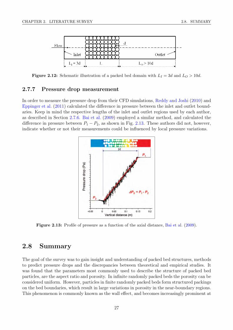
CHAPTER 2. LITERATURE SURVEY 2.8. SUMMARY
Figure 2.12: Schematic illustration of a packed bed domain with LI = 3d and LO > 10d.
2.7.7 Pressure drop measurement
In order to measure the pressure drop from their CFD simulations, Reddy and Joshi (2010) andEppinger et al. (2011) calculated the difference in pressure between the inlet and outlet bound-aries. Keep in mind the respective lengths of the inlet and outlet regions used by each author,as described in Section 2.7.6. Bai et al. (2009) employed a similar method, and calculated thedifference in pressure between P1 − P2, as shown in Fig. 2.13. These authors did not, however,indicate whether or not their measurements could be influenced by local pressure variations.
Figure 2.13: Profile of pressure as a function of the axial distance, Bai et al. (2009).
2.8 Summary
The goal of the survey was to gain insight and understanding of packed bed structures, methodsto predict pressure drops and the discrepancies between theoretical and empirical studies. Itwas found that the parameters most commonly used to describe the structure of packed bedparticles, are the aspect ratio and porosity. In infinite randomly packed beds the porosity can beconsidered uniform. However, particles in finite randomly packed beds form structured packingson the bed boundaries, which result in large variations in porosity in the near-boundary regions.This phenomenon is commonly known as the wall effect, and becomes increasingly prominent at
27
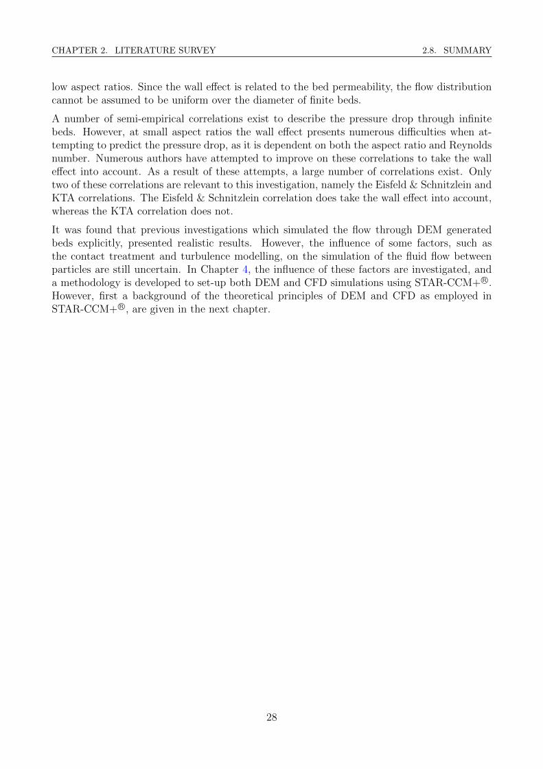
CHAPTER 2. LITERATURE SURVEY 2.8. SUMMARY
low aspect ratios. Since the wall effect is related to the bed permeability, the flow distributioncannot be assumed to be uniform over the diameter of finite beds.
A number of semi-empirical correlations exist to describe the pressure drop through infinitebeds. However, at small aspect ratios the wall effect presents numerous difficulties when at-tempting to predict the pressure drop, as it is dependent on both the aspect ratio and Reynoldsnumber. Numerous authors have attempted to improve on these correlations to take the walleffect into account. As a result of these attempts, a large number of correlations exist. Onlytwo of these correlations are relevant to this investigation, namely the Eisfeld & Schnitzlein andKTA correlations. The Eisfeld & Schnitzlein correlation does take the wall effect into account,whereas the KTA correlation does not.
It was found that previous investigations which simulated the flow through DEM generatedbeds explicitly, presented realistic results. However, the influence of some factors, such asthe contact treatment and turbulence modelling, on the simulation of the fluid flow betweenparticles are still uncertain. In Chapter 4, the influence of these factors are investigated, anda methodology is developed to set-up both DEM and CFD simulations using STAR-CCM+ R©.However, first a background of the theoretical principles of DEM and CFD as employed inSTAR-CCM+ R©, are given in the next chapter.
28
Chapter 3
Modelling theory
Both Discrete Element Modelling and Computational Fluid Dynamics form an integral partof this investigation. In this chapter, the basic theoretical principles of DEM and CFD aredescribed, as they are employed in STAR-CCM+ R©. Note that these principles are describedonly briefly, and more detailed information can be found in CD-Adapco (2012) and Versteegand Malalasekera (2007).
3.1 Discrete Element Modelling
First introduced by Cundall and Strack (1979), Discrete Element Modelling (DEM) is an ex-plicit numerical scheme which simulates the dynamic and static behaviour of assemblies ofparticles based on contact mechanics. It is usually assumed that particles displace indepen-dently, interact only at contact points and are rigid bodies. In STAR-CCM+ R©, DEM is anextension of Lagrangian modelling methodology which includes dense particle flows. The dis-tinct characteristic is that inter-particle contact forces are included in the equations of motion.STAR-CCM+ R© uses a classical mechanics method to model DEM, which is based on a softparticle approach. The particles are allowed to develop a minute overlap that is proportionalto the calculated contact force. The contact force is thus proportional to the overlap, particlematerial and geometric properties (CD-Adapco, 2012).
3.1.1 Momentum balance
The momentum balance for DEM particles is derived from the momentum balance of materialparticles, eq. (3.1). The DEM model introduces an extra body force representing inter-particleinteractions due to contacts between particles and between particles and boundaries, eq. (3.2).
mp ·dUpdt
= (FS) + (FB) (3.1)
= (Fd + Fpg + Fvm) + (Fg + Fud + Fsct) (3.2)
In eq. (3.1), mp is the mass of a particle, Up is the velocity of that particle, and FS and FB
29
CHAPTER 3. MODELLING THEORY 3.1. DISCRETE ELEMENT MODELLING
represent the the forces acting on the surface of the particle and the body forces respectively.In eq. (3.2), Fd is the drag force, Fpg is the pressure gradient force, Fvm is a virtual mass force,Fg is the gravity force and Fud is a user-defined body force. For detail on each of these forcessee CD-Adapco (2012, p. 4343). Fsct is the sum of the contact forces acting on a particle:
Fsct =Neighbour∑Particles
Fct +Neighbour∑Boundaries
Fct (3.3)
where Fct is the contact force by particle-particle or particle-boundary interactions. It shouldbe noted that the exact formulation of contact forces is controlled by a user specified contactmodel. These contact models are described in the next section.
3.1.2 Contact force modelling
STAR-CCM+ R© provides the Hertz-Mindlin no-slip model for modelling the forces at contactpoints. The formulation of contact forces in STAR-CCM+ R© is a variant of the non-linearspring-dashpot model. The spring represents the forces which push particles apart, and thedashpot represents viscous damping and allows collision types other than perfectly elastic tobe simulated. The forces between two particles are described as:
Fct = Fn + Ft (3.4)
where Fn is the force component in the normal direction and Ft the force component in thetangential direction. The forces in the normal direction is defined as:
Fn = −Kndno − JnUnp (3.5)
where K is the spring stiffness, do the particle overlap and J the damping coefficient. Similarly,the forces in the tangential direction is:
Ft =
−Ktdto − J tU t
p if |Kndno |Cfs > |Ktdto|KndnoCfsd
to/|dto| if |Kndno |Cfs ≤ |Ktdto|
(3.6)
where Cfs is a static friction coefficient. Note that Kn, Kt and J are all functions of an equiv-alent Young’s modulus, equivalent shear modulus, equivalent particle diameter and equivalentparticle mass. For particle-boundary collisions the Hertz-Mindlin model remains unchanged.However, the boundary diameter and mass are assumed to the infinite, which reduces theequivalent diameter and mass to only that of the particle. CD-Adapco (2012) states thatthe resulting code of the Hertz-Mindlin contact model is computationally efficient while stillmatching experimental data.
30
CHAPTER 3. MODELLING THEORY 3.2. COMPUTATIONAL FLUID DYNAMICS
3.2 Computational Fluid Dynamics
Computational Fluid Dynamics (CFD) is the analysis of systems involving fluid flow, heattransfer and associated phenomena by means of computer based simulations (Versteeg andMalalasekera, 2007). In order to simulate these phenomena, the conservation laws of physicsmust be upheld (Versteeg and Malalasekera, 2007, p. 9):
1. The mass of a fluid is conserved.
2. The rate of change of momentum equals the sum of the forces on a fluid particle (Newton’ssecond law).
3. The rate of change of energy is equal to the sum of the rate of heat addition to and therate of work done on a fluid particle (first law of thermodynamics).
This section describes the equations which are based on these laws, and how they are discretizedand applied to a finite number of control volumes.
3.2.1 Transport equations
The mechanics of physics continua are described by transport equations derived from the as-sumption that mass, momentum, energy and entropy are conserved in the continuum. Thetransport equation for a general variable φ can be written as:
∂ρφ
∂t+∇ · (ρφu) = ∇ · (Γ∇φ) + Sφ (3.7)
where u is the vector velocity field, Γ a the diffusion coefficient, ∇ the del operator and Sφ allthe source terms for the property φ. In words, eq. (3.7) is:
Rate of change of φ. + Convective term. = Diffusion term. + Source terms.
By setting φ equal to 1, u, v, w and ν respectively, and selecting appropriate values for Γ andsource terms, the system of equations which govern the time-dependent three-dimensional fluidflow and heat transfer of a compressible Newtonian fluid can be obtained:
∂ρ
∂t+∇ · (ρu) = 0 (3.8)
∂ρu
∂t+∇ · (ρuu) = −∂p
∂x+∇ · (µ∇u) + Sx (3.9)
∂ρv
∂t+∇ · (ρvu) = −∂p
∂y+∇ · (µ∇v) + Sy (3.10)
∂ρw
∂t+∇ · (ρwu) = −∂p
∂z+∇ · (µ∇w) + Sz (3.11)
31
CHAPTER 3. MODELLING THEORY 3.2. COMPUTATIONAL FLUID DYNAMICS
∂ρν
∂t+∇ · (ρνu) = −p∇ · u +∇ · (κ∇T ) + Υ + Sν (3.12)
p = p (ρ, T ) ; ν = ν (ρ, T ) (3.13)
Eq. (3.8) is the continuity equation. Eqns. (3.9), (3.10) and (3.11), also known as the Navier-Stokes equations, are the momentum equations in the x, y and z directions respectively andu, v and w the components of u. Eq. (3.12) is the energy equation with ν the specific internalenergy, κ the conduction heat transfer coefficient and Υ a dissipation function. Eq. (3.13)represents the equations of state which relate other variables to the two state variables, ρ andT , where T is the fluid temperature. Eqns. (3.8) to (3.13) are the governing equations of theconservation laws of physics for fluid flow.
3.2.2 Finite volume method
In order to apply the governing equations of the conservation laws of physics to a solutiondomain, the domain is discredized into a finite number of non-overlapping control volumes.These control volumes correspond to the cells of a computational grid. The gaol is to obtain aset of algebraic equations, which can be solved using an algebraic multi-grid solver. First, eq.(3.7) is integrated over one of these control volumes, labelled λ:
∫V
∂ρφ
∂tdV +
∫V∇ · (ρφu) dV =
∫V∇ · (Γ∇φ) dV +
∫VSφ dV (3.14)
where V is the volume of the control volume λ. When considering a steady state calculation,the first term equates to zero. Applying Gauss’s divergence theorem to the convection anddiffusion terms give:
∫∂V
(ρφu) · dS =∫∂V
(Γ∇φ) · dS +∫VSφ dV (3.15)
where ∂V is the control volume boundary and dS an outward pointing surface vector on saidboundary. The control volume consists of ϑ flat faces, thus the surface integral can be decom-posed as the sum of the integrals over the different faces that surrounds the control volume:
ϑ∑ϕ=1
∫ϕ
(ρφu) · dS =ϑ∑
ϕ=1
∫ϕ
(Γ∇φ) · dS +∫VSφ dV (3.16)
where ϕ is the control volume face number. For continuous functions under the integrals, themidpoint integration rule can now be applied to the integrals:
ϑ∑ϕ=1
(ρφu)ϕ ·Aϕ =ϑ∑
ϕ=1
(Γ∇φ)ϕ ·Aϕ + (SφV )λ (3.17)
32

CHAPTER 3. MODELLING THEORY 3.2. COMPUTATIONAL FLUID DYNAMICS
where A is the outward pointing face area vector. The face number and the centre of the facesare labelled with the subscript ϕ. For continuous flow properties the values of the individualproperties can be interpolated to the faces:
ϑ∑ϕ=1
ρϕφϕuϕ ·Aϕ =ϑ∑
ϕ=1
Γϕ (∇φ)ϕ ·Aϕ + (SφV )λ (3.18)
Eq. (3.18) is the discrete form of eq. (3.7) for a steady state calculation as employed in STAR-CCM+ R©.
3.2.3 Turbulence
Many flows of engineering significance are turbulent, however the random nature of turbulentflow presents a challenge when attempting to simulate the turbulent regime. This section givesa brief introduction to the modelling of turbulence as employed in STAR-CCM+ R©.
RANS turbulence models
To obtain the Reynolds-Average Navier-Stokes (RANS) equations, the Navier-Stokes equations,eqns. (3.9) to (3.11), are time averaged and decomposed into a mean value and a fluctuatingcomponent. The resulting equations for the mean values are essentially identical to the originalequations, however an additional term appears on the right hand side of the momentum trans-port equations. This additional term is known as the Reynolds stress tensor, and representsthe fluctuating component. Written in the form of eq. (3.7), the RANS equations are:
∂ρ̄Φ
∂t+∇ · (ρ̄ΦU) = ∇ · (Γ∇Φ) + T + SΦ (3.19)
u = U + u′ ; Φ =1
∆t·∫ ∆t
0φ(t) dt (3.20)
where U and u′ are the mean and fluctuating components of u respectively, Φ the time averageof the property φ, t the time, and the over-bar indicates time averaged. The Reynolds stresstensor, T, is:
T = −∂(ρu′φ′)
∂x− ∂(ρv′φ′)
∂y− ∂(ρw′φ′)
∂z(3.21)
where φ′ is the fluctuating component of φ. The challenge is thus to model the Reynoldsstress tensor in terms of mean flow quantities. One of the most widely used methods is to usethe turbulent viscosity, µτ , to model T. These models are known as eddy-viscosity models.Presently, the k− ε models are the most widely used and validated of all eddy-viscosity models(Versteeg and Malalasekera, 2007, p. 67). Many variations of the model exist, however thecommon principle between all k − ε models is that a velocity scale/intensity, γ, and lengthscale, `, are defined which represent the large scale turbulence:
33
CHAPTER 3. MODELLING THEORY 3.2. COMPUTATIONAL FLUID DYNAMICS
γ = γ (k) ; ` = ` (k, ε) (3.22)
where k is the turbulent kinetic energy and ε the turbulent dissipation rate. The turbulentviscosity used to model T is then:
µτ = µτ (ρkε) ; T = T (µτρk) (3.23)
In STAR-CCM+ R© the eddy-viscosity models also solve additional transport equations for quan-tities such as k and ε to derive µτ .
Large Eddy Simulation
LES is an inherently transient technique which solves the behaviour of large 3D eddies, whilethe effects of small eddies on the flow are treated using sub-grid models. The equations solvedfor LES are obtained through a filtering process of the unsteady Navier-Stokes equations. Thefiltered equations look similar to the unsteady RANS equations, however T now represents thesub-grid scale stresses. This tensor is modelled using the Boussinesq approximation:
T = 2µτS− 2
3(µτ∇ · u + ρk) δ (3.24)
where S is a strain rate tensor and δ a function similar to the Kronecker delta.
Note that one of the difficulties with LES is defining appropriate turbulent conditions at inletboundaries. STAR-CCM+ R© uses a Synthetic Eddy Method (SEM) to automatically provideturbulent eddies across inlet boundaries.
3.2.4 Mesh generation
Generating a proper mesh is an integral part of any CFD simulation, since the quality anddensity of the mesh have a great impact on the stability and accuracy of the solution. STAR-CCM+ R© contains tools which can be used to generate a volume mesh, starting from a surface.The volume mesh is the mathematical description of the domain of the problem being solved.It is in turn constructed of the following:
1. Vertices.A vertex is a point in space defined by a position vector.
2. Faces.A face consists of an ordered collection of vertices, such that they define a 3D surface.Faces may have any number of vertices.
3. Cells.A cell is an ordered collection of faces, which define a closed volume. These cells arethe control volumes to which the transport equations, eq. (3.18), are applied. Cells mayhave any number of faces, as long as it contains enough faces to create a closed volume.
34

CHAPTER 3. MODELLING THEORY 3.3. SUMMARY
Cells of arbitrary polyhedral shape are also permitted, which allows for the generation ofunstructured meshes.
The mesh parameters, such as meshing models and cell sizes, are contained within mesh con-tinua. STAR-CCM+ R© allows many meshing parameters to be set, and many are specific tocertain meshing models, however the most basic parameters are:
1. Base size, B.The base size value is a characteristic dimension of the geometry of the problem beingsolved. Usually, all other properties are set relative to the base size.
2. Surface size.The surface size allows values to be set which determine the resultant size of the cellsnext to the surfaces of the domain. It is usually set with a target and minimum size,where the target value is the desired edge cell length on the surface, and the minimumvalue controls the lower limit of the edge cell length.
3. Surface growth rate.The surface growth rate controls the rate at which the lengths of cell edges can vary fromone cell to its neighbour. This parameter is useful when local refinement of the volumemesh is required.
Rough meshes often lead to unstable and inaccurate solutions, while dense meshes demandmore computational resources. In any CFD simulation, a compromise must be made betweenthe accuracy of the results and the time and effort needed for an accurate solution. CD-Adapco(2012, p. 1902) also notes that it is likely that several iterations might be required to obtainappropriate mesh parameters for a simulation.
3.3 Summary
In this chapter, the basic theoretical principles of DEM and CFD were described, as theyare employed in STAR-CCM+ R©. The momentum balance for DEM particles was given, andthe modelling of contact forces between particles was described. The analytical form of thetransport equations necessary to simulate fluid flow within a control volume was shown. Thediscrete form of these equations, as applied to a finite number of control volumes or cells, wasderived. The basic principles of turbulence modelling and mesh generation were also described.In the next chapter a methodology is developed to simulate the flow through DEM generatedbeds explicitly using STAR-CCM+ R©. These simulations employ the principles described inthis chapter.
35
Chapter 4
Methodology
This chapter describes the steps taken during the numerical analyses of the flow through packedbeds, to ensure accurate solutions with a reasonable degree of confidence. The commercial CFDpackage STAR-CCM+ R© was used for all analyses, as Preller (2011) and Theron (2011) provedthat STAR-CCM+ R© is an appropriate platform to generate packed beds using DEM, andperforming CFD analysis of the flow through packed beds.
4.1 DEM simulation setup
This section contains detail on the DEM simulation setup which was used to generate all thebeds needed for the CFD simulations of the flow through the beds. The default values for therelevant parameters in STAR-CCM+ R© version 7.06 were used, unless stated otherwise.
4.1.1 Geometry and boundaries
Simple cylindrical domains were created using SolidWorks, which were imported into STAR-CCM+ R© as surface meshes. These domains had diameters equal to the cylinder diameters ofthe final beds, D, and axial lengths of LDEM . See Section 4.1.2 for more detail on LDEM . Thecylinder- and particle surfaces were set as wall boundaries, with no slip.
4.1.2 Particle injection
To accommodate particle generation, LDEM was made 20% larger than the expected length ofthe final bed, L. Thus, LDEM = 1.2d (L/d), where L/d = 10. The L/d relation is describedin more detail in Section 4.8. Particles were generated at the top of the domain using a pointinjector, and simulated to fall in the z-direction with a gravitational acceleration of −9.81 m/s2.The point injector was set on the cylinder centreline, one particle diameter from the top surfaceof the cylinder. Particles were generated at a rate of one particle per second.
36
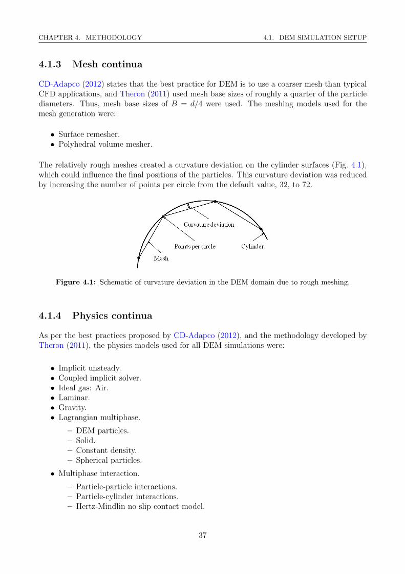
CHAPTER 4. METHODOLOGY 4.1. DEM SIMULATION SETUP
4.1.3 Mesh continua
CD-Adapco (2012) states that the best practice for DEM is to use a coarser mesh than typicalCFD applications, and Theron (2011) used mesh base sizes of roughly a quarter of the particlediameters. Thus, mesh base sizes of B = d/4 were used. The meshing models used for themesh generation were:
• Surface remesher.• Polyhedral volume mesher.
The relatively rough meshes created a curvature deviation on the cylinder surfaces (Fig. 4.1),which could influence the final positions of the particles. This curvature deviation was reducedby increasing the number of points per circle from the default value, 32, to 72.
Figure 4.1: Schematic of curvature deviation in the DEM domain due to rough meshing.
4.1.4 Physics continua
As per the best practices proposed by CD-Adapco (2012), and the methodology developed byTheron (2011), the physics models used for all DEM simulations were:
• Implicit unsteady.• Coupled implicit solver.• Ideal gas: Air.• Laminar.• Gravity.• Lagrangian multiphase.
– DEM particles.– Solid.– Constant density.– Spherical particles.
• Multiphase interaction.
– Particle-particle interactions.– Particle-cylinder interactions.– Hertz-Mindlin no slip contact model.
37
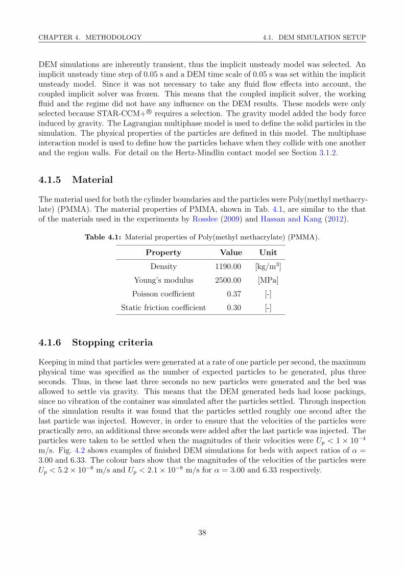
CHAPTER 4. METHODOLOGY 4.1. DEM SIMULATION SETUP
DEM simulations are inherently transient, thus the implicit unsteady model was selected. Animplicit unsteady time step of 0.05 s and a DEM time scale of 0.05 s was set within the implicitunsteady model. Since it was not necessary to take any fluid flow effects into account, thecoupled implicit solver was frozen. This means that the coupled implicit solver, the workingfluid and the regime did not have any influence on the DEM results. These models were onlyselected because STAR-CCM+ R© requires a selection. The gravity model added the body forceinduced by gravity. The Lagrangian multiphase model is used to define the solid particles in thesimulation. The physical properties of the particles are defined in this model. The multiphaseinteraction model is used to define how the particles behave when they collide with one anotherand the region walls. For detail on the Hertz-Mindlin contact model see Section 3.1.2.
4.1.5 Material
The material used for both the cylinder boundaries and the particles were Poly(methyl methacry-late) (PMMA). The material properties of PMMA, shown in Tab. 4.1, are similar to the thatof the materials used in the experiments by Rosslee (2009) and Hassan and Kang (2012).
Table 4.1: Material properties of Poly(methyl methacrylate) (PMMA).
Property Value Unit
Density 1190.00 [kg/m3]
Young’s modulus 2500.00 [MPa]
Poisson coefficient 0.37 [-]
Static friction coefficient 0.30 [-]
4.1.6 Stopping criteria
Keeping in mind that particles were generated at a rate of one particle per second, the maximumphysical time was specified as the number of expected particles to be generated, plus threeseconds. Thus, in these last three seconds no new particles were generated and the bed wasallowed to settle via gravity. This means that the DEM generated beds had loose packings,since no vibration of the container was simulated after the particles settled. Through inspectionof the simulation results it was found that the particles settled roughly one second after thelast particle was injected. However, in order to ensure that the velocities of the particles werepractically zero, an additional three seconds were added after the last particle was injected. Theparticles were taken to be settled when the magnitudes of their velocities were Up < 1 × 10⁻⁴
m/s. Fig. 4.2 shows examples of finished DEM simulations for beds with aspect ratios of α =3.00 and 6.33. The colour bars show that the magnitudes of the velocities of the particles wereUp < 5.2× 10⁻⁸ m/s and Up < 2.1× 10⁻⁸ m/s for α = 3.00 and 6.33 respectively.
38

CHAPTER 4. METHODOLOGY 4.2. CFD SIMULATION SETUP
(a) α = 3.00. (b) α = 6.33.
Figure 4.2: Examples of finished DEM simulations with particle velocities practically zero.
4.2 CFD simulation setup
This section contains detail on the CFD simulation setup which was used to simulate the flowthrough the beds. The default values for the relevant parameters in STAR-CCM+ R© version7.06 were used, unless stated otherwise.
4.2.1 Geometry
Domains for the CFD simulations of the flow through the beds were created using SolidWorks,by importing the centre coordinates of the particles obtained from the DEM simulations. Thisstep was necessary since the version of STAR-CCM+ R© used for this investigation was not yetcapable of converting DEM particles to solid bodies. The version used also did not providethe tools needed for contact treatment, whereas SolidWorks did. Figs. 4.3a and 4.3b show twoexamples of these domains as created in SolidWorks, for beds with aspect ratios of α = 3.00and α = 6.33 respectively.
(a) α = 3.00. (b) α = 6.33.
Figure 4.3: Examples of domains used for CFD simulations created in SolidWorks.
The domains were created with inlet and outlet regions as described in Section 2.7.6, with theinlet region extending a length of LI = 3d from the bed and the outlet region extending a
39
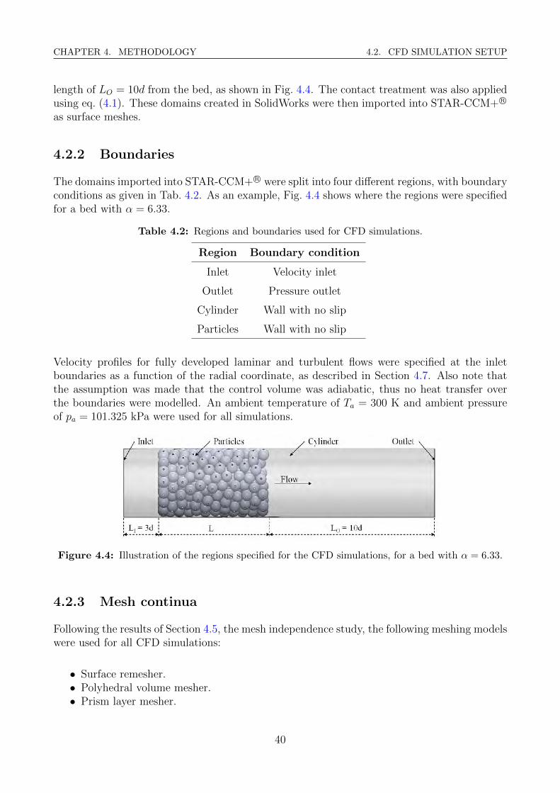
CHAPTER 4. METHODOLOGY 4.2. CFD SIMULATION SETUP
length of LO = 10d from the bed, as shown in Fig. 4.4. The contact treatment was also appliedusing eq. (4.1). These domains created in SolidWorks were then imported into STAR-CCM+ R©
as surface meshes.
4.2.2 Boundaries
The domains imported into STAR-CCM+ R© were split into four different regions, with boundaryconditions as given in Tab. 4.2. As an example, Fig. 4.4 shows where the regions were specifiedfor a bed with α = 6.33.
Table 4.2: Regions and boundaries used for CFD simulations.
Region Boundary condition
Inlet Velocity inlet
Outlet Pressure outlet
Cylinder Wall with no slip
Particles Wall with no slip
Velocity profiles for fully developed laminar and turbulent flows were specified at the inletboundaries as a function of the radial coordinate, as described in Section 4.7. Also note thatthe assumption was made that the control volume was adiabatic, thus no heat transfer overthe boundaries were modelled. An ambient temperature of Ta = 300 K and ambient pressureof pa = 101.325 kPa were used for all simulations.
Figure 4.4: Illustration of the regions specified for the CFD simulations, for a bed with α = 6.33.
4.2.3 Mesh continua
Following the results of Section 4.5, the mesh independence study, the following meshing modelswere used for all CFD simulations:
• Surface remesher.• Polyhedral volume mesher.• Prism layer mesher.
40
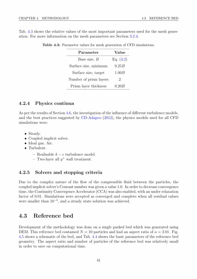
CHAPTER 4. METHODOLOGY 4.3. REFERENCE BED
Tab. 4.3 shows the relative values of the most important parameters used for the mesh gener-ation. For more information on the mesh parameters see Section 3.2.4.
Table 4.3: Parameter values for mesh generation of CFD simulations.
Parameter Value
Base size, B Eq. (4.2)
Surface size, minimum 0.25B
Surface size, target 1.00B
Number of prism layers 2
Prism layer thickness 0.20B
4.2.4 Physics continua
As per the results of Section 4.6, the investigation of the influence of different turbulence models,and the best practices suggested by CD-Adapco (2012), the physics models used for all CFDsimulations were:
• Steady.• Coupled implicit solver.• Ideal gas: Air.• Turbulent.
– Realisable k − ε turbulence model.– Two-layer all y+ wall treatment.
4.2.5 Solvers and stopping criteria
Due to the complex nature of the flow of the compressible fluid between the particles, thecoupled implicit solver’s Courant number was given a value 1.0. In order to decrease convergencetime, the Continuity Convergence Accelerator (CCA) was also enabled, with an under relaxationfactor of 0.01. Simulations were accepted as converged and complete when all residual valueswere smaller than 10−3, and a steady state solution was achieved.
4.3 Reference bed
Development of the methodology was done on a single packed bed which was generated usingDEM. This reference bed contained N = 10 particles and had an aspect ratio of α = 2.01. Fig.4.5 shows a schematic of the bed, and Tab. 4.4 shows the basic parameters of the reference bedgeometry. The aspect ratio and number of particles of the reference bed was relatively smallin order to save on computational time.
41
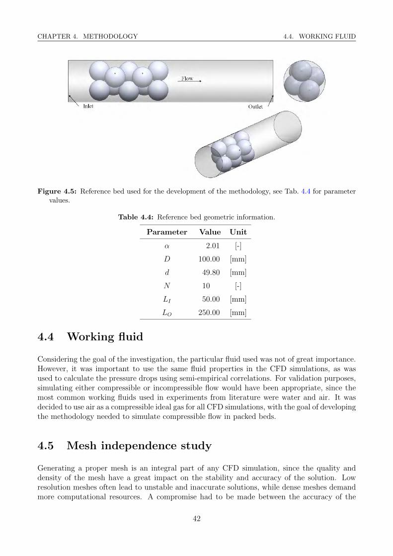
CHAPTER 4. METHODOLOGY 4.4. WORKING FLUID
Figure 4.5: Reference bed used for the development of the methodology, see Tab. 4.4 for parametervalues.
Table 4.4: Reference bed geometric information.
Parameter Value Unit
α 2.01 [-]
D 100.00 [mm]
d 49.80 [mm]
N 10 [-]
LI 50.00 [mm]
LO 250.00 [mm]
4.4 Working fluid
Considering the goal of the investigation, the particular fluid used was not of great importance.However, it was important to use the same fluid properties in the CFD simulations, as wasused to calculate the pressure drops using semi-empirical correlations. For validation purposes,simulating either compressible or incompressible flow would have been appropriate, since themost common working fluids used in experiments from literature were water and air. It wasdecided to use air as a compressible ideal gas for all CFD simulations, with the goal of developingthe methodology needed to simulate compressible flow in packed beds.
4.5 Mesh independence study
Generating a proper mesh is an integral part of any CFD simulation, since the quality anddensity of the mesh have a great impact on the stability and accuracy of the solution. Lowresolution meshes often lead to unstable and inaccurate solutions, while dense meshes demandmore computational resources. A compromise had to be made between the accuracy of the
42
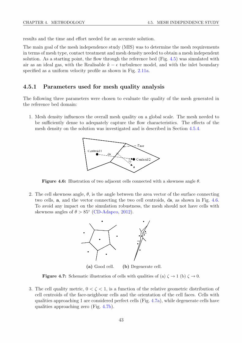
CHAPTER 4. METHODOLOGY 4.5. MESH INDEPENDENCE STUDY
results and the time and effort needed for an accurate solution.
The main goal of the mesh independence study (MIS) was to determine the mesh requirementsin terms of mesh type, contact treatment and mesh density needed to obtain a mesh independentsolution. As a starting point, the flow through the reference bed (Fig. 4.5) was simulated withair as an ideal gas, with the Realisable k − ε turbulence model, and with the inlet boundaryspecified as a uniform velocity profile as shown in Fig. 2.11a.
4.5.1 Parameters used for mesh quality analysis
The following three parameters were chosen to evaluate the quality of the mesh generated inthe reference bed domain:
1. Mesh density influences the overall mesh quality on a global scale. The mesh needed tobe sufficiently dense to adequately capture the flow characteristics. The effects of themesh density on the solution was investigated and is described in Section 4.5.4.
Figure 4.6: Illustration of two adjacent cells connected with a skewness angle θ.
2. The cell skewness angle, θ, is the angle between the area vector of the surface connectingtwo cells, a, and the vector connecting the two cell centroids, ds, as shown in Fig. 4.6.To avoid any impact on the simulation robustness, the mesh should not have cells withskewness angles of θ > 85◦ (CD-Adapco, 2012).
(a) Good cell. (b) Degenerate cell.
Figure 4.7: Schematic illustration of cells with qualities of (a) ζ → 1 (b) ζ → 0.
3. The cell quality metric, 0 < ζ < 1, is a function of the relative geometric distribution ofcell centroids of the face-neighbour cells and the orientation of the cell faces. Cells withqualities approaching 1 are considered perfect cells (Fig. 4.7a), while degenerate cells havequalities approaching zero (Fig. 4.7b).
43
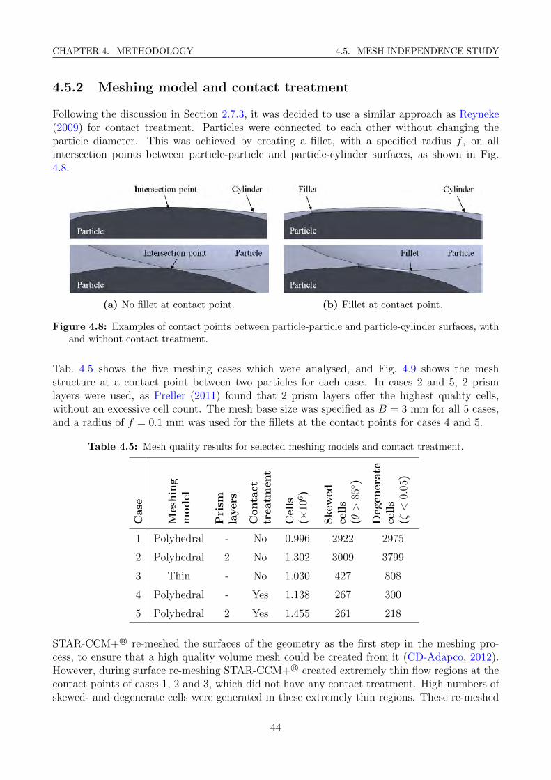
CHAPTER 4. METHODOLOGY 4.5. MESH INDEPENDENCE STUDY
4.5.2 Meshing model and contact treatment
Following the discussion in Section 2.7.3, it was decided to use a similar approach as Reyneke(2009) for contact treatment. Particles were connected to each other without changing theparticle diameter. This was achieved by creating a fillet, with a specified radius f , on allintersection points between particle-particle and particle-cylinder surfaces, as shown in Fig.4.8.
(a) No fillet at contact point. (b) Fillet at contact point.
Figure 4.8: Examples of contact points between particle-particle and particle-cylinder surfaces, withand without contact treatment.
Tab. 4.5 shows the five meshing cases which were analysed, and Fig. 4.9 shows the meshstructure at a contact point between two particles for each case. In cases 2 and 5, 2 prismlayers were used, as Preller (2011) found that 2 prism layers offer the highest quality cells,without an excessive cell count. The mesh base size was specified as B = 3 mm for all 5 cases,and a radius of f = 0.1 mm was used for the fillets at the contact points for cases 4 and 5.
Table 4.5: Mesh quality results for selected meshing models and contact treatment.
Case
Mesh
ing
model
Pri
smla
yers
Conta
cttr
eatm
ent
Cells
(×10
6)
Skew
ed
cells
(θ>
85◦ )
Degenera
tece
lls
(ζ<
0.05
)
1 Polyhedral - No 0.996 2922 2975
2 Polyhedral 2 No 1.302 3009 3799
3 Thin - No 1.030 427 808
4 Polyhedral - Yes 1.138 267 300
5 Polyhedral 2 Yes 1.455 261 218
STAR-CCM+ R© re-meshed the surfaces of the geometry as the first step in the meshing pro-cess, to ensure that a high quality volume mesh could be created from it (CD-Adapco, 2012).However, during surface re-meshing STAR-CCM+ R© created extremely thin flow regions at thecontact points of cases 1, 2 and 3, which did not have any contact treatment. High numbers ofskewed- and degenerate cells were generated in these extremely thin regions. These re-meshed
44

CHAPTER 4. METHODOLOGY 4.5. MESH INDEPENDENCE STUDY
surfaces also created gaps between particles which would negatively influence the simulation ofheat transfer between particles. From Tab. 4.5 it can be seen that case 5 had the least numberof skewed cells with θ > 85◦, as well as the least number of low quality cells with ζ < 0.05.The use of 2 prism layers increased the cell count, however according to CD-Adapco (2012),prism layers greatly enhance the accuracy of the simulation as they are necessary to simulateboundary layers.
(a) Case 1. (b) Case 2. (c) Case 3. (d) Case 4. (e) Case 5.
Figure 4.9: Mesh structure at a contact point between two particles, as per Tab. 4.5.
With these results, as well as the recommendations of Dixon et al. (2013) in Section 2.7.3, case5 was chosen as the primary meshing method, with a polyhedral meshing model, 2 prism layersand fillets created at the contact points.
4.5.3 Contact area
Fig. 4.10 shows schematically that specifying a fillet, with a radius f , at the contact pointbetween two particles also inherently specifies the size of the diameter of the contact area, DC ,and the contact area itself, C.
Figure 4.10: Schematic illustration of a contact point between two particles with a filler radius f .
Though the influence of the contact area on the heat transfer between particles was not analysedin this investigation, it will be an important factor for future studies considering the temperaturedistributions within packed beds. The influence of the size of the contact point fillet on the
45

CHAPTER 4. METHODOLOGY 4.5. MESH INDEPENDENCE STUDY
pressure drop was investigated. The flow through the reference bed was simulated with fivedifferent values for f , as shown in Fig. 4.11. The mesh base size was specified as B = 2 mmfor all five cases, which resulted in roughly 1.359 × 10⁶ cells. Tab. 4.6 shows the five differentvalues used for f , as well as their corresponding contact diameters, DC , and contact areas, C.
(a) f = 0.05 mm. (b) f = 0.1 mm. (c) f = 0.2 mm. (d) f = 0.4 mm. (e) f = 0.8 mm.
Figure 4.11: Mesh structure at a contact point between two particles for different values of f .
Table 4.6: Corresponding values between f , DC , and C.
f [mm] 0.05 0.10 0.20 0.40 0.80
DC [mm] 3.21 4.38 6.00 8.22 11.16
C [mm2] 8.09 15.07 28.27 53.07 97.82
Fig. 4.12a shows that the pressure drop increased for f > 0.1 mm, due to the increased flowrestriction, and increased for f < 0.1 mm, due to low cell quality in the contact region. Thus,fillets with f = 0.1 mm had the smallest influence on the fluid flow, while still limiting thenumber of low quality cells. A fillet radius of f = 0.1 mm was chosen for the reference bed,however in order to scale the fillet radius to beds with different aspect ratios, f was calculatedas a percentage of the particle diameter:
f =0.2d
100(4.1)
4.5.4 Mesh density
The influence of the mesh density on the simulation was analysed by simulating the flow throughthe reference bed, while decreasing the mesh base size, B, and consequently increasing the cellcount and mesh density. Fig. 4.12b shows that the pressure drop over the bed was meshindependent above roughly 1.2× 10⁶ cells, since the pressure drop ∆p (B = 2) was within 1.0%of ∆p (B = 1.4). In order to have a mesh independent solution without an excessive cell count,a mesh density which corresponded to 1.7 ≤ B ≤ 2 mm was chosen for the reference bed. Fig.4.13 shows the structure of the mesh in the reference bed, with B = 2 mm. In order to scale
46
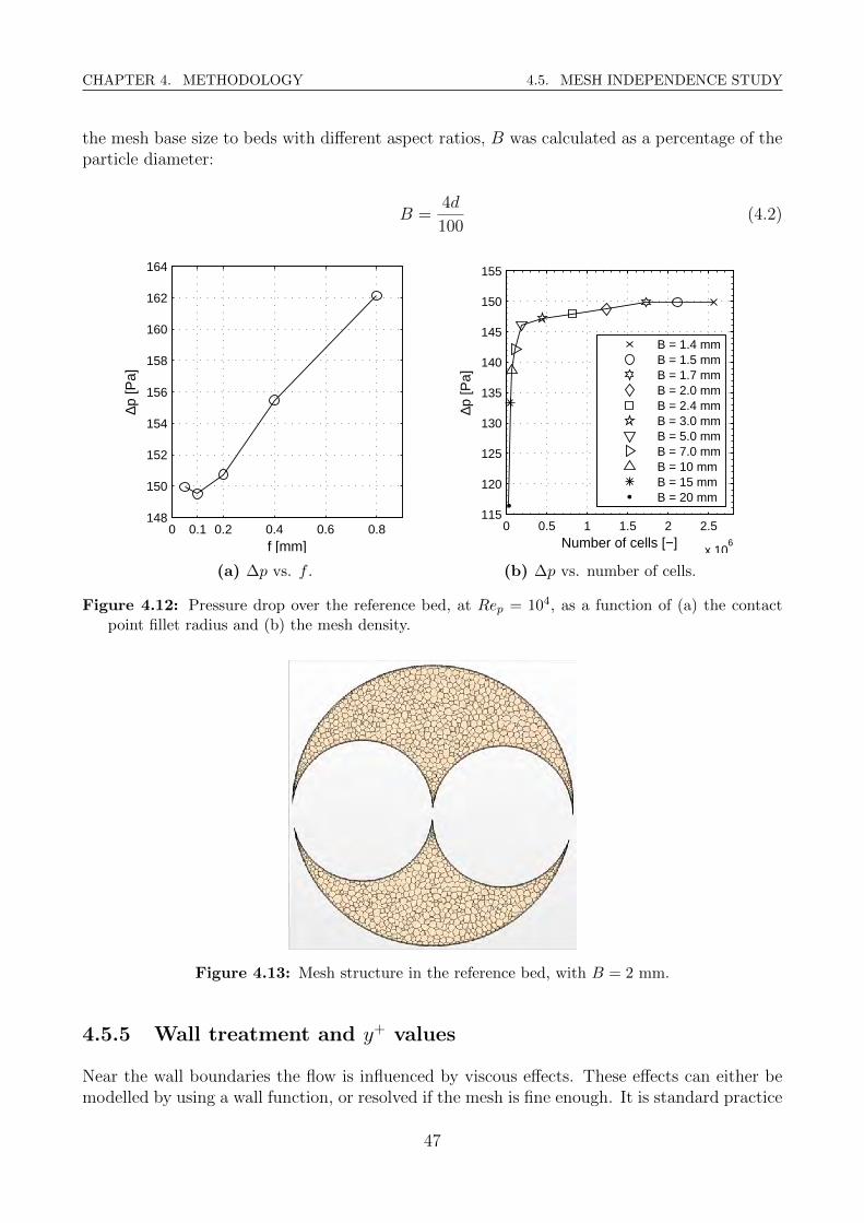
CHAPTER 4. METHODOLOGY 4.5. MESH INDEPENDENCE STUDY
the mesh base size to beds with different aspect ratios, B was calculated as a percentage of theparticle diameter:
B =4d
100(4.2)
0 0.1 0.2 0.4 0.6 0.8148
150
152
154
156
158
160
162
164
∆p [P
a]
f [mm]
(a) ∆p vs. f .
0 0.5 1 1.5 2 2.5
x 106
115
120
125
130
135
140
145
150
155
∆p [P
a]
Number of cells [−]
B = 1.4 mmB = 1.5 mmB = 1.7 mmB = 2.0 mmB = 2.4 mmB = 3.0 mmB = 5.0 mmB = 7.0 mmB = 10 mmB = 15 mmB = 20 mm
(b) ∆p vs. number of cells.
Figure 4.12: Pressure drop over the reference bed, at Rep = 104, as a function of (a) the contactpoint fillet radius and (b) the mesh density.
Figure 4.13: Mesh structure in the reference bed, with B = 2 mm.
4.5.5 Wall treatment and y+ values
Near the wall boundaries the flow is influenced by viscous effects. These effects can either bemodelled by using a wall function, or resolved if the mesh is fine enough. It is standard practice
47
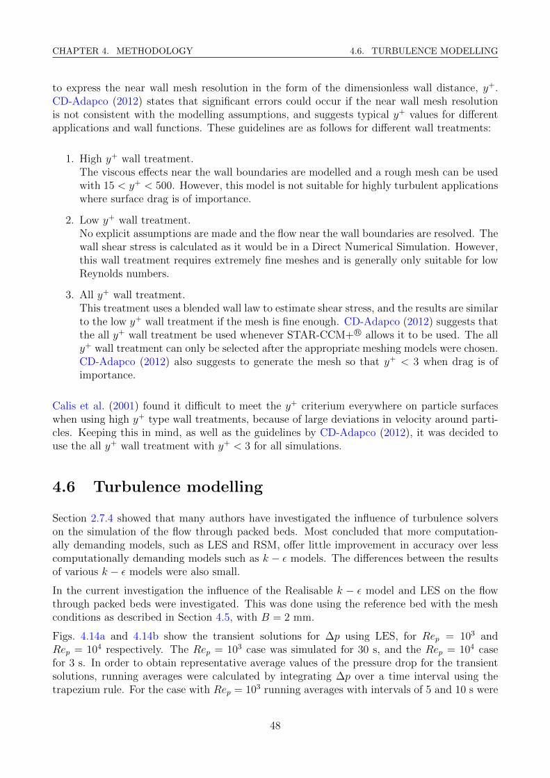
CHAPTER 4. METHODOLOGY 4.6. TURBULENCE MODELLING
to express the near wall mesh resolution in the form of the dimensionless wall distance, y+.CD-Adapco (2012) states that significant errors could occur if the near wall mesh resolutionis not consistent with the modelling assumptions, and suggests typical y+ values for differentapplications and wall functions. These guidelines are as follows for different wall treatments:
1. High y+ wall treatment.The viscous effects near the wall boundaries are modelled and a rough mesh can be usedwith 15 < y+ < 500. However, this model is not suitable for highly turbulent applicationswhere surface drag is of importance.
2. Low y+ wall treatment.No explicit assumptions are made and the flow near the wall boundaries are resolved. Thewall shear stress is calculated as it would be in a Direct Numerical Simulation. However,this wall treatment requires extremely fine meshes and is generally only suitable for lowReynolds numbers.
3. All y+ wall treatment.This treatment uses a blended wall law to estimate shear stress, and the results are similarto the low y+ wall treatment if the mesh is fine enough. CD-Adapco (2012) suggests thatthe all y+ wall treatment be used whenever STAR-CCM+ R© allows it to be used. The ally+ wall treatment can only be selected after the appropriate meshing models were chosen.CD-Adapco (2012) also suggests to generate the mesh so that y+ < 3 when drag is ofimportance.
Calis et al. (2001) found it difficult to meet the y+ criterium everywhere on particle surfaceswhen using high y+ type wall treatments, because of large deviations in velocity around parti-cles. Keeping this in mind, as well as the guidelines by CD-Adapco (2012), it was decided touse the all y+ wall treatment with y+ < 3 for all simulations.
4.6 Turbulence modelling
Section 2.7.4 showed that many authors have investigated the influence of turbulence solverson the simulation of the flow through packed beds. Most concluded that more computation-ally demanding models, such as LES and RSM, offer little improvement in accuracy over lesscomputationally demanding models such as k − ε models. The differences between the resultsof various k − ε models were also small.
In the current investigation the influence of the Realisable k − ε model and LES on the flowthrough packed beds were investigated. This was done using the reference bed with the meshconditions as described in Section 4.5, with B = 2 mm.
Figs. 4.14a and 4.14b show the transient solutions for ∆p using LES, for Rep = 103 andRep = 104 respectively. The Rep = 103 case was simulated for 30 s, and the Rep = 104 casefor 3 s. In order to obtain representative average values of the pressure drop for the transientsolutions, running averages were calculated by integrating ∆p over a time interval using thetrapezium rule. For the case with Rep = 103 running averages with intervals of 5 and 10 s were
48
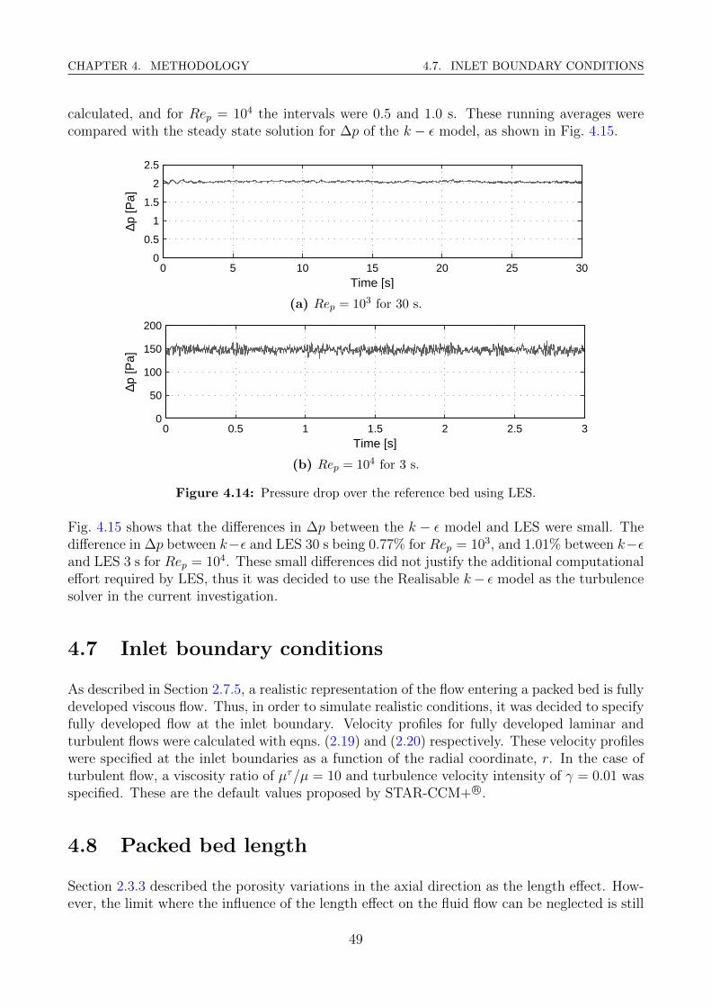
CHAPTER 4. METHODOLOGY 4.7. INLET BOUNDARY CONDITIONS
calculated, and for Rep = 104 the intervals were 0.5 and 1.0 s. These running averages werecompared with the steady state solution for ∆p of the k − ε model, as shown in Fig. 4.15.
0 5 10 15 20 25 300
0.5
1
1.5
2
2.5
∆p [P
a]
Time [s]
(a) Rep = 103 for 30 s.
0 0.5 1 1.5 2 2.5 30
50
100
150
200
∆p [P
a]
Time [s]
(b) Rep = 104 for 3 s.
Figure 4.14: Pressure drop over the reference bed using LES.
Fig. 4.15 shows that the differences in ∆p between the k − ε model and LES were small. Thedifference in ∆p between k−ε and LES 30 s being 0.77% for Rep = 103, and 1.01% between k−εand LES 3 s for Rep = 104. These small differences did not justify the additional computationaleffort required by LES, thus it was decided to use the Realisable k− ε model as the turbulencesolver in the current investigation.
4.7 Inlet boundary conditions
As described in Section 2.7.5, a realistic representation of the flow entering a packed bed is fullydeveloped viscous flow. Thus, in order to simulate realistic conditions, it was decided to specifyfully developed flow at the inlet boundary. Velocity profiles for fully developed laminar andturbulent flows were calculated with eqns. (2.19) and (2.20) respectively. These velocity profileswere specified at the inlet boundaries as a function of the radial coordinate, r. In the case ofturbulent flow, a viscosity ratio of µτ/µ = 10 and turbulence velocity intensity of γ = 0.01 wasspecified. These are the default values proposed by STAR-CCM+ R©.
4.8 Packed bed length
Section 2.3.3 described the porosity variations in the axial direction as the length effect. How-ever, the limit where the influence of the length effect on the fluid flow can be neglected is still
49
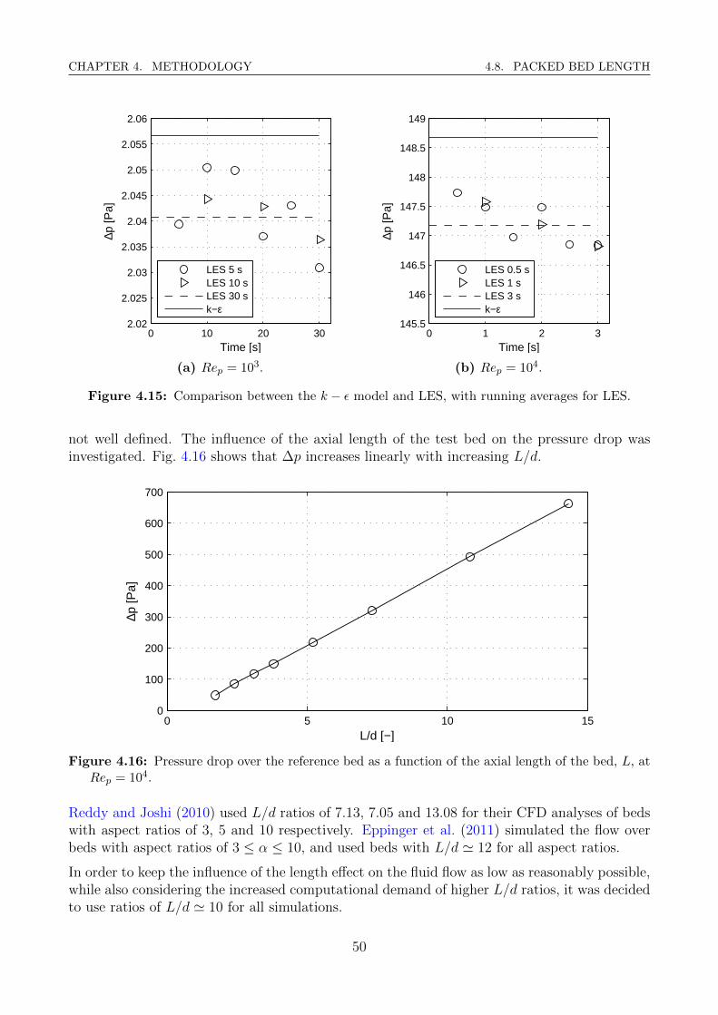
CHAPTER 4. METHODOLOGY 4.8. PACKED BED LENGTH
0 10 20 302.02
2.025
2.03
2.035
2.04
2.045
2.05
2.055
2.06∆p
[Pa]
Time [s]
LES 5 sLES 10 sLES 30 sk−ε
(a) Rep = 103.
0 1 2 3145.5
146
146.5
147
147.5
148
148.5
149
∆p [P
a]
Time [s]
LES 0.5 sLES 1 sLES 3 sk−ε
(b) Rep = 104.
Figure 4.15: Comparison between the k − ε model and LES, with running averages for LES.
not well defined. The influence of the axial length of the test bed on the pressure drop wasinvestigated. Fig. 4.16 shows that ∆p increases linearly with increasing L/d.
0 5 10 150
100
200
300
400
500
600
700
∆p [P
a]
L/d [−]
Figure 4.16: Pressure drop over the reference bed as a function of the axial length of the bed, L, atRep = 104.
Reddy and Joshi (2010) used L/d ratios of 7.13, 7.05 and 13.08 for their CFD analyses of bedswith aspect ratios of 3, 5 and 10 respectively. Eppinger et al. (2011) simulated the flow overbeds with aspect ratios of 3 ≤ α ≤ 10, and used beds with L/d ' 12 for all aspect ratios.
In order to keep the influence of the length effect on the fluid flow as low as reasonably possible,while also considering the increased computational demand of higher L/d ratios, it was decidedto use ratios of L/d ' 10 for all simulations.
50
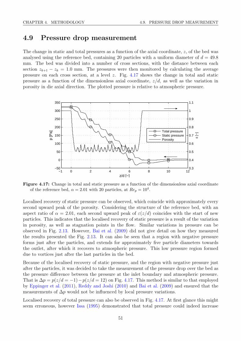
CHAPTER 4. METHODOLOGY 4.9. PRESSURE DROP MEASUREMENT
4.9 Pressure drop measurement
The change in static and total pressures as a function of the axial coordinate, z, of the bed wasanalysed using the reference bed, containing 20 particles with a uniform diameter of d = 49.8mm. The bed was divided into a number of cross sections, with the distance between eachsection zk+1 − zk = 1.0 mm. The pressures were then monitored by calculating the averagepressure on each cross section, at a level z. Fig. 4.17 shows the change in total and staticpressure as a function of the dimensionless axial coordinate, z/d, as well as the variation inporosity in die axial direction. The plotted pressure is relative to atmospheric pressure.
−1 0 2 4 6 8 10 12−50
0
50
100
150
200
250
300
350
z/d [−]
p [P
a]
Total pressureStatic pressurePorosity
0.3
0.4
0.5
0.6
0.7
0.8
0.9
1
1.1
ε [−
]
Figure 4.17: Change in total and static pressure as a function of the dimensionless axial coordinateof the reference bed, α = 2.01 with 20 particles, at Rep = 104.
Localised recovery of static pressure can be observed, which coincide with approximately everysecond upward peak of the porosity. Considering the structure of the reference bed, with anaspect ratio of α = 2.01, each second upward peak of ε(z/d) coincides with the start of newparticles. This indicates that the localised recovery of static pressure is a result of the variationin porosity, as well as stagnation points in the flow. Similar variations in pressure can beobserved in Fig. 2.13. However, Bai et al. (2009) did not give detail on how they measuredthe results presented the Fig. 2.13. It can also be seen that a region with negative pressureforms just after the particles, and extends for approximately five particle diameters towardsthe outlet, after which it recovers to atmospheric pressure. This low pressure region formeddue to vortices just after the last particles in the bed.
Because of the localised recovery of static pressure, and the region with negative pressure justafter the particles, it was decided to take the measurement of the pressure drop over the bed asthe pressure difference between the pressure at the inlet boundary and atmospheric pressure.That is ∆p = p(z/d = −1)−p(z/d = 12) on Fig. 4.17. This method is similar to that employedby Eppinger et al. (2011), Reddy and Joshi (2010) and Bai et al. (2009) and ensured that themeasurements of ∆p would not be influenced by local pressure variations.
Localised recovery of total pressure can also be observed in Fig. 4.17. At first glance this mightseem erroneous, however Issa (1995) demonstrated that total pressure could indeed increase
51
CHAPTER 4. METHODOLOGY 4.10. SUMMARY
in turbulent, viscid flows, particularly around stagnation points. Issa (1995) also noted thatlocalised rises of total pressure can only occur at the expense of depletion of total pressureelsewhere in the flow, as mechanical energy stays conserved. Thus, the localised recovery oftotal pressure can also be attributed to the variation in porosity and stagnation points in theflow. The consequences that these local rises of total pressure may have on the flow throughpacked beds, however, fall beyond the scope of the current investigation. Further analysis willbe needed to determine the influence that these rises might have on the temperature distributionwithin packed beds.
The recovery of total pressure between the last particles and the outlet in Fig. 4.17, could bea result of vortices forming after the particles, as the energy contained in the vortices may notbe properly accounted for with total pressure. However, this increase might also be due to theoutlet boundary having an effect on the upstream flow.
4.10 Summary
This chapter described the steps taken during the numerical analyses of the flow through packedbeds, to ensure accurate solutions with a reasonable degree of confidence. Preller (2011) andTheron (2011) proved that STAR-CCM+ R© is an appropriate platform to generate packed bedsusing DEM, and performing CFD analysis of the flow through packed beds. This chapterextended on the work done by Theron (2011).
Detail of the setup used for the DEM simulations to generate all the beds was given, as well asdetail of the setup used for the CFD simulations of the flow through the beds. The geometryof the reference bed was described, which was used to analyse the influence of some key factorson the simulation of the fluid flow between particles. These factors included the mesh density,contact treatment, turbulence modelling, boundary conditions and measurement of the pressuredrop. The influence of these factors on the simulations was also described in detail. Themethods developed and setups described in this chapter were used to simulate the flow throughDEM generated packed beds explicitly. The results of these simulations are presented in thenext chapter.
52
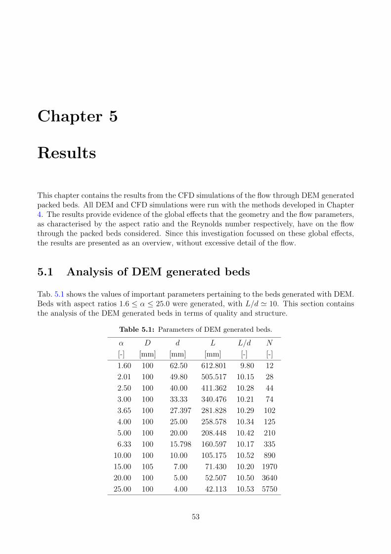
Chapter 5
Results
This chapter contains the results from the CFD simulations of the flow through DEM generatedpacked beds. All DEM and CFD simulations were run with the methods developed in Chapter4. The results provide evidence of the global effects that the geometry and the flow parameters,as characterised by the aspect ratio and the Reynolds number respectively, have on the flowthrough the packed beds considered. Since this investigation focussed on these global effects,the results are presented as an overview, without excessive detail of the flow.
5.1 Analysis of DEM generated beds
Tab. 5.1 shows the values of important parameters pertaining to the beds generated with DEM.Beds with aspect ratios 1.6 ≤ α ≤ 25.0 were generated, with L/d ' 10. This section containsthe analysis of the DEM generated beds in terms of quality and structure.
Table 5.1: Parameters of DEM generated beds.
α D d L L/d N
[-] [mm] [mm] [mm] [-] [-]
1.60 100 62.50 612.801 9.80 12
2.01 100 49.80 505.517 10.15 28
2.50 100 40.00 411.362 10.28 44
3.00 100 33.33 340.476 10.21 74
3.65 100 27.397 281.828 10.29 102
4.00 100 25.00 258.578 10.34 125
5.00 100 20.00 208.448 10.42 210
6.33 100 15.798 160.597 10.17 335
10.00 100 10.00 105.175 10.52 890
15.00 105 7.00 71.430 10.20 1970
20.00 100 5.00 52.507 10.50 3640
25.00 100 4.00 42.113 10.53 5750
53

CHAPTER 5. RESULTS 5.1. ANALYSIS OF DEM GENERATED BEDS
5.1.1 Particle overlaps
The quality of the DEM generated beds were assessed by calculating the overlap, do, betweenadjacent particles (Du Toit and Rosslee, 2012). Ideally there should be no overlap. The distancedij between spheres i and j was calculated using eq. (5.1), where xi, yi, zi and xj, yj, zj arethe coordinates of the centres of the spheres. The percentage overlap, do, was then calculatedusing eq. (5.2), and Fig. 5.1a shows the maximum and minimum overlaps. It can be seen thatthe overlaps between adjacent particles in the beds generated using DEM were small, withdo,max < 0.08% for all beds.
dij =√
(xi − xj)2 + (yi − yj)2 + (zi − zj)2 (5.1)
do =
(d− dij)× 100/d for d > dij
0 for d ≤ dij(5.2)
0 5 10 15 20 250
0.01
0.02
0.03
0.04
0.05
0.06
0.07
0.08
d o [%]
α [−]
MaximumAverage
(a) Overlap between particles.
0 5 10 15 20 250
0.02
0.04
0.06
0.08
0.1
∆εb [%
]
α [−]
(b) Difference between eqns. (2.3) and (2.6).
Figure 5.1: Quality analysis of the DEM generated packed beds, with values given in Tab. 5.1.
5.1.2 Porosity and structure
Bulk porosities were calculated with both the analytical expression of Bai et al. (2009), eq. (2.3),and the numerical expression of Du Toit and Rosslee (2012), eq. (2.6). These porosities werecalculated taking z1 as the lowest and zn−1 as the highest point in the bed, and ∆z = 0.01d.Fig. 5.1b shows the percentage difference between these calculated bulk porosities. It can beseen that there is a good agreement between the analytically and numerically calculated valuesfor εb, where ∆εb < 0.1% for all beds. Note that the numerical solution tended to the analyticalsolution as ∆z → 0.
54
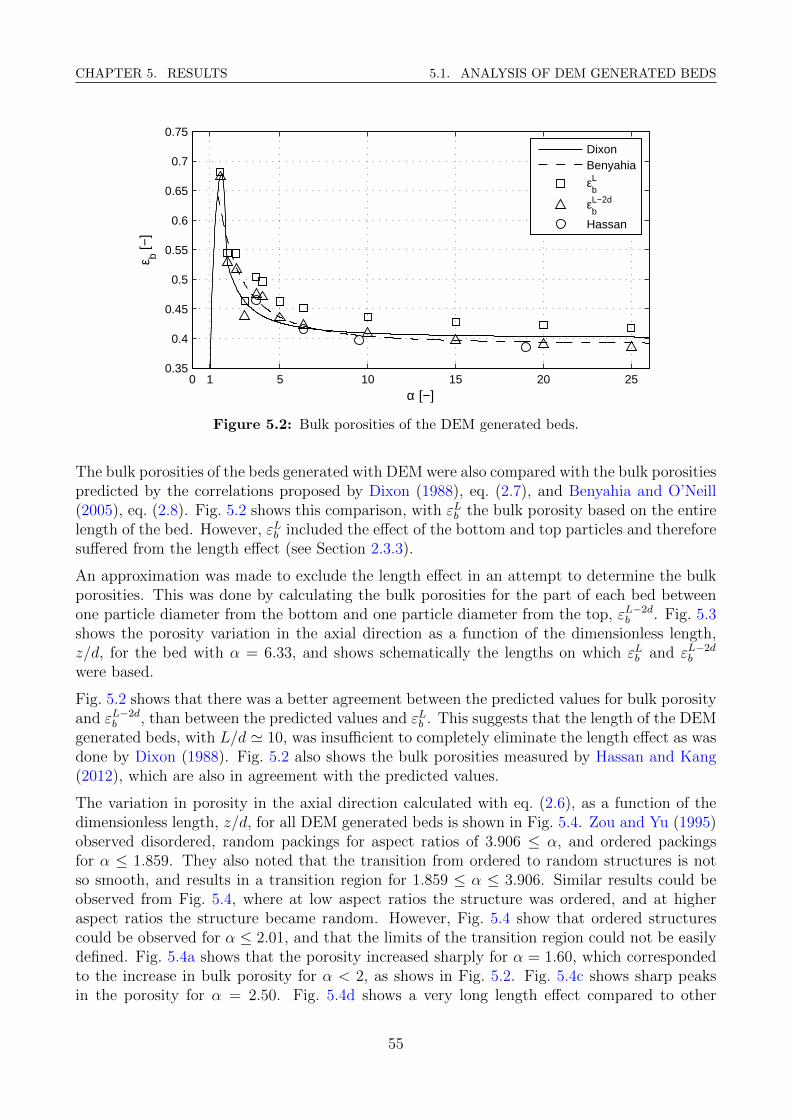
CHAPTER 5. RESULTS 5.1. ANALYSIS OF DEM GENERATED BEDS
0 1 5 10 15 20 250.35
0.4
0.45
0.5
0.55
0.6
0.65
0.7
0.75ε b [−
]
α [−]
DixonBenyahia
εbL
εbL−2d
Hassan
Figure 5.2: Bulk porosities of the DEM generated beds.
The bulk porosities of the beds generated with DEM were also compared with the bulk porositiespredicted by the correlations proposed by Dixon (1988), eq. (2.7), and Benyahia and O’Neill(2005), eq. (2.8). Fig. 5.2 shows this comparison, with εLb the bulk porosity based on the entirelength of the bed. However, εLb included the effect of the bottom and top particles and thereforesuffered from the length effect (see Section 2.3.3).
An approximation was made to exclude the length effect in an attempt to determine the bulkporosities. This was done by calculating the bulk porosities for the part of each bed betweenone particle diameter from the bottom and one particle diameter from the top, εL−2d
b . Fig. 5.3shows the porosity variation in the axial direction as a function of the dimensionless length,z/d, for the bed with α = 6.33, and shows schematically the lengths on which εLb and εL−2d
b
were based.
Fig. 5.2 shows that there was a better agreement between the predicted values for bulk porosityand εL−2d
b , than between the predicted values and εLb . This suggests that the length of the DEMgenerated beds, with L/d ' 10, was insufficient to completely eliminate the length effect as wasdone by Dixon (1988). Fig. 5.2 also shows the bulk porosities measured by Hassan and Kang(2012), which are also in agreement with the predicted values.
The variation in porosity in the axial direction calculated with eq. (2.6), as a function of thedimensionless length, z/d, for all DEM generated beds is shown in Fig. 5.4. Zou and Yu (1995)observed disordered, random packings for aspect ratios of 3.906 ≤ α, and ordered packingsfor α ≤ 1.859. They also noted that the transition from ordered to random structures is notso smooth, and results in a transition region for 1.859 ≤ α ≤ 3.906. Similar results could beobserved from Fig. 5.4, where at low aspect ratios the structure was ordered, and at higheraspect ratios the structure became random. However, Fig. 5.4 show that ordered structurescould be observed for α ≤ 2.01, and that the limits of the transition region could not be easilydefined. Fig. 5.4a shows that the porosity increased sharply for α = 1.60, which correspondedto the increase in bulk porosity for α < 2, as shows in Fig. 5.2. Fig. 5.4c shows sharp peaksin the porosity for α = 2.50. Fig. 5.4d shows a very long length effect compared to other
55
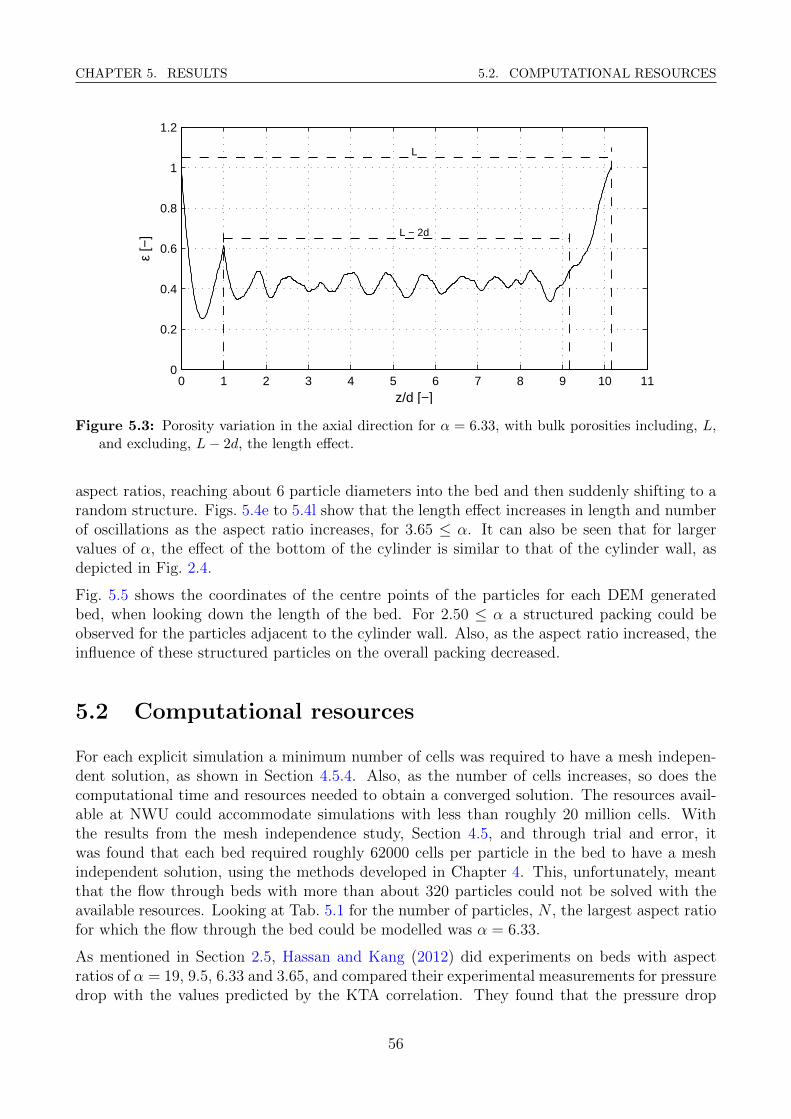
CHAPTER 5. RESULTS 5.2. COMPUTATIONAL RESOURCES
0 1 2 3 4 5 6 7 8 9 10 110
0.2
0.4
0.6
0.8
1
1.2ε
[−]
z/d [−]
L − 2d
L
Figure 5.3: Porosity variation in the axial direction for α = 6.33, with bulk porosities including, L,and excluding, L− 2d, the length effect.
aspect ratios, reaching about 6 particle diameters into the bed and then suddenly shifting to arandom structure. Figs. 5.4e to 5.4l show that the length effect increases in length and numberof oscillations as the aspect ratio increases, for 3.65 ≤ α. It can also be seen that for largervalues of α, the effect of the bottom of the cylinder is similar to that of the cylinder wall, asdepicted in Fig. 2.4.
Fig. 5.5 shows the coordinates of the centre points of the particles for each DEM generatedbed, when looking down the length of the bed. For 2.50 ≤ α a structured packing could beobserved for the particles adjacent to the cylinder wall. Also, as the aspect ratio increased, theinfluence of these structured particles on the overall packing decreased.
5.2 Computational resources
For each explicit simulation a minimum number of cells was required to have a mesh indepen-dent solution, as shown in Section 4.5.4. Also, as the number of cells increases, so does thecomputational time and resources needed to obtain a converged solution. The resources avail-able at NWU could accommodate simulations with less than roughly 20 million cells. Withthe results from the mesh independence study, Section 4.5, and through trial and error, itwas found that each bed required roughly 62000 cells per particle in the bed to have a meshindependent solution, using the methods developed in Chapter 4. This, unfortunately, meantthat the flow through beds with more than about 320 particles could not be solved with theavailable resources. Looking at Tab. 5.1 for the number of particles, N , the largest aspect ratiofor which the flow through the bed could be modelled was α = 6.33.
As mentioned in Section 2.5, Hassan and Kang (2012) did experiments on beds with aspectratios of α = 19, 9.5, 6.33 and 3.65, and compared their experimental measurements for pressuredrop with the values predicted by the KTA correlation. They found that the pressure drop
56
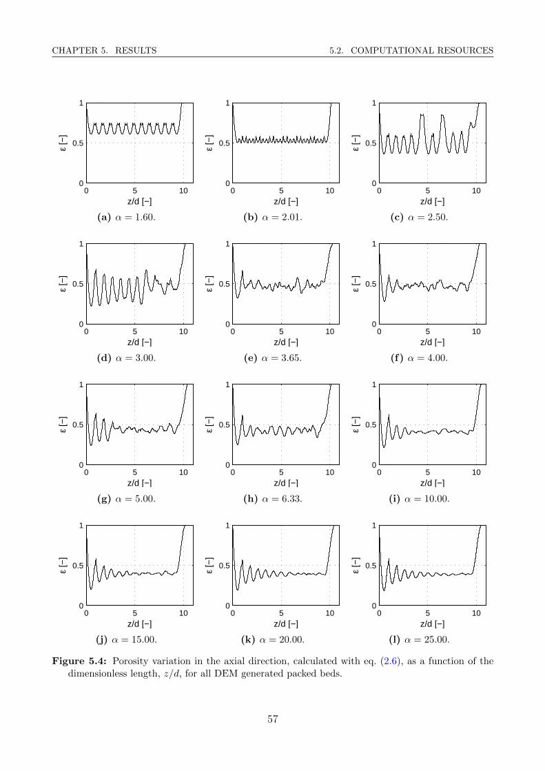
CHAPTER 5. RESULTS 5.2. COMPUTATIONAL RESOURCES
0 5 100
0.5
1
ε [−
]
z/d [−]
(a) α = 1.60.
0 5 100
0.5
1
ε [−
]z/d [−]
(b) α = 2.01.
0 5 100
0.5
1
ε [−
]
z/d [−]
(c) α = 2.50.
0 5 100
0.5
1
ε [−
]
z/d [−]
(d) α = 3.00.
0 5 100
0.5
1
ε [−
]
z/d [−]
(e) α = 3.65.
0 5 100
0.5
1
ε [−
]z/d [−]
(f) α = 4.00.
0 5 100
0.5
1
ε [−
]
z/d [−]
(g) α = 5.00.
0 5 100
0.5
1
ε [−
]
z/d [−]
(h) α = 6.33.
0 5 100
0.5
1
ε [−
]
z/d [−]
(i) α = 10.00.
0 5 100
0.5
1
ε [−
]
z/d [−]
(j) α = 15.00.
0 5 100
0.5
1
ε [−
]
z/d [−]
(k) α = 20.00.
0 5 100
0.5
1
ε [−
]
z/d [−]
(l) α = 25.00.
Figure 5.4: Porosity variation in the axial direction, calculated with eq. (2.6), as a function of thedimensionless length, z/d, for all DEM generated packed beds.
57
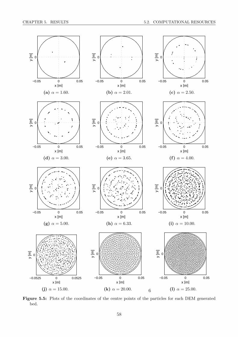
CHAPTER 5. RESULTS 5.2. COMPUTATIONAL RESOURCES
−0.05 0 0.05
0
y [m
]
x [m]
(a) α = 1.60.
−0.05 0 0.05
0
y [m
]
x [m]
(b) α = 2.01.
−0.05 0 0.05
0
y [m
]
x [m]
(c) α = 2.50.
−0.05 0 0.05
0
y [m
]
x [m]
(d) α = 3.00.
−0.05 0 0.05
0
y [m
]
x [m]
(e) α = 3.65.
−0.05 0 0.05
0
y [m
]x [m]
(f) α = 4.00.
−0.05 0 0.05
0
y [m
]
x [m]
(g) α = 5.00.
−0.05 0 0.05
0
y [m
]
x [m]
(h) α = 6.33.
−0.05 0 0.05
0
y [m
]
x [m]
(i) α = 10.00.
−0.0525 0 0.0525
0
y [m
]
x [m]
(j) α = 15.00.
−0.05 0 0.05
0
y [m
]
x [m]
(k) α = 20.00. 6
−0.05 0 0.05
0
y [m
]
x [m]
(l) α = 25.00.
Figure 5.5: Plots of the coordinates of the centre points of the particles for each DEM generatedbed.
58
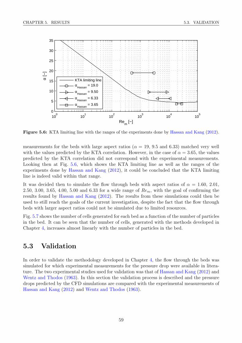
CHAPTER 5. RESULTS 5.3. VALIDATION
100
101
102
103
104
105
0
5
10
15
20
25
30
35
Rem
[−]
α [−
]
KTA limiting lineα
Hassan = 19.0
αHassan
= 9.50
αHassan
= 6.33
αHassan
= 3.65
Figure 5.6: KTA limiting line with the ranges of the experiments done by Hassan and Kang (2012).
measurements for the beds with large aspect ratios (α = 19, 9.5 and 6.33) matched very wellwith the values predicted by the KTA correlation. However, in the case of α = 3.65, the valuespredicted by the KTA correlation did not correspond with the experimental measurements.Looking then at Fig. 5.6, which shows the KTA limiting line as well as the ranges of theexperiments done by Hassan and Kang (2012), it could be concluded that the KTA limitingline is indeed valid within that range.
It was decided then to simulate the flow through beds with aspect ratios of α = 1.60, 2.01,2.50, 3.00, 3.65, 4.00, 5.00 and 6.33 for a wide range of Rem, with the goal of confirming theresults found by Hassan and Kang (2012). The results from these simulations could then beused to still reach the goals of the current investigation, despite the fact that the flow throughbeds with larger aspect ratios could not be simulated due to limited resources.
Fig. 5.7 shows the number of cells generated for each bed as a function of the number of particlesin the bed. It can be seen that the number of cells, generated with the methods developed inChapter 4, increases almost linearly with the number of particles in the bed.
5.3 Validation
In order to validate the methodology developed in Chapter 4, the flow through the beds wassimulated for which experimental measurements for the pressure drop were available in litera-ture. The two experimental studies used for validation was that of Hassan and Kang (2012) andWentz and Thodos (1963). In this section the validation process is described and the pressuredrops predicted by the CFD simulations are compared with the experimental measurements ofHassan and Kang (2012) and Wentz and Thodos (1963).
59
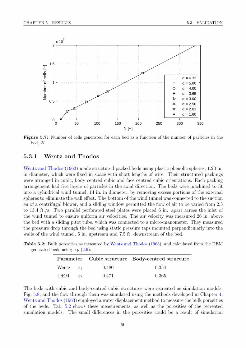
CHAPTER 5. RESULTS 5.3. VALIDATION
0 50 100 150 200 250 300 3500
0.5
1
1.5
2x 10
7
Num
ber
of c
ells
[−]
N [−]
α = 6.33α = 5.00α = 4.00α = 3.65α = 3.00α = 2.50α = 2.01α = 1.60
Figure 5.7: Number of cells generated for each bed as a function of the number of particles in thebed, N .
5.3.1 Wentz and Thodos
Wentz and Thodos (1963) made structured packed beds using plastic phenolic spheres, 1.23 in.in diameter, which were fixed in space with short lengths of wire. Their structured packingswere arranged in cubic, body centred cubic and face centred cubic orientations. Each packingarrangement had five layers of particles in the axial direction. The beds were machined to fitinto a cylindrical wind tunnel, 14 in. in diameter, by removing excess portions of the externalspheres to eliminate the wall effect. The bottom of the wind tunnel was connected to the suctionen of a centrifugal blower, and a sliding window permitted the flow of air to be varied from 2.5to 13.4 ft./s. Two parallel perforated steel plates were placed 6 in. apart across the inlet ofthe wind tunnel to ensure uniform air velocities. The air velocity was measured 26 in. abovethe bed with a sliding pitot tube, which was connected to a micro-manometer. They measuredthe pressure drop through the bed using static pressure taps mounted perpendicularly into thewalls of the wind tunnel, 5 in. upstream and 7.5 ft. downstream of the bed.
Table 5.2: Bulk porosities as measured by Wentz and Thodos (1963), and calculated from the DEMgenerated beds using eq. (2.6).
Parameter Cubic structure Body-centred structure
Wentz εb 0.480 0.354
DEM εb 0.471 0.365
The beds with cubic and body-centred cubic structures were recreated as simulation models,Fig. 5.8, and the flow through them was simulated using the methods developed in Chapter 4.Wentz and Thodos (1963) employed a water displacement method to measure the bulk porositiesof the beds. Tab. 5.2 shows these measurements, as well as the porosities of the recreatedsimulation models. The small differences in the porosities could be a result of simulation
60
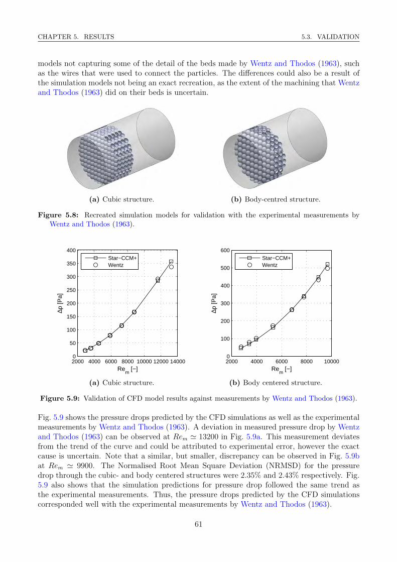
CHAPTER 5. RESULTS 5.3. VALIDATION
models not capturing some of the detail of the beds made by Wentz and Thodos (1963), suchas the wires that were used to connect the particles. The differences could also be a result ofthe simulation models not being an exact recreation, as the extent of the machining that Wentzand Thodos (1963) did on their beds is uncertain.
(a) Cubic structure. (b) Body-centred structure.
Figure 5.8: Recreated simulation models for validation with the experimental measurements byWentz and Thodos (1963).
2000 4000 6000 8000 10000 12000 140000
50
100
150
200
250
300
350
400
∆p [P
a]
Rem
[−]
Star−CCM+Wentz
(a) Cubic structure.
2000 4000 6000 8000 100000
100
200
300
400
500
600
∆p [P
a]
Rem
[−]
Star−CCM+Wentz
(b) Body centered structure.
Figure 5.9: Validation of CFD model results against measurements by Wentz and Thodos (1963).
Fig. 5.9 shows the pressure drops predicted by the CFD simulations as well as the experimentalmeasurements by Wentz and Thodos (1963). A deviation in measured pressure drop by Wentzand Thodos (1963) can be observed at Rem ' 13200 in Fig. 5.9a. This measurement deviatesfrom the trend of the curve and could be attributed to experimental error, however the exactcause is uncertain. Note that a similar, but smaller, discrepancy can be observed in Fig. 5.9bat Rem ' 9900. The Normalised Root Mean Square Deviation (NRMSD) for the pressuredrop through the cubic- and body centered structures were 2.35% and 2.43% respectively. Fig.5.9 also shows that the simulation predictions for pressure drop followed the same trend asthe experimental measurements. Thus, the pressure drops predicted by the CFD simulationscorresponded well with the experimental measurements by Wentz and Thodos (1963).
61
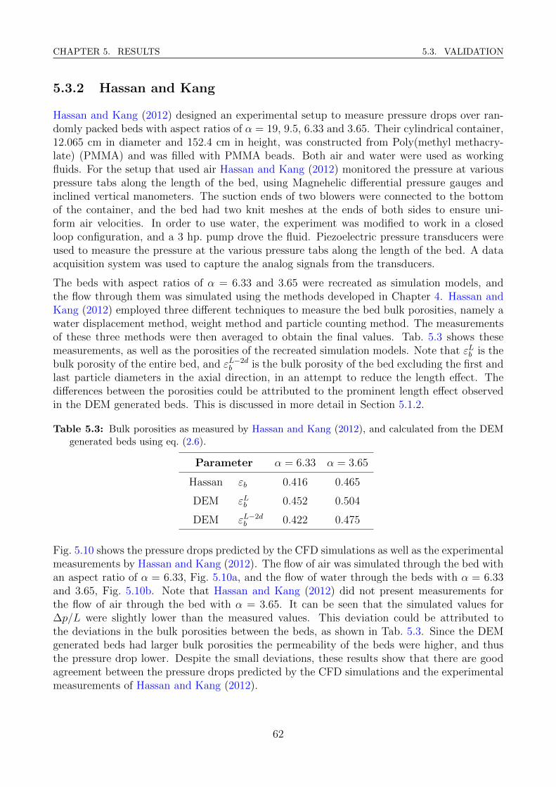
CHAPTER 5. RESULTS 5.3. VALIDATION
5.3.2 Hassan and Kang
Hassan and Kang (2012) designed an experimental setup to measure pressure drops over ran-domly packed beds with aspect ratios of α = 19, 9.5, 6.33 and 3.65. Their cylindrical container,12.065 cm in diameter and 152.4 cm in height, was constructed from Poly(methyl methacry-late) (PMMA) and was filled with PMMA beads. Both air and water were used as workingfluids. For the setup that used air Hassan and Kang (2012) monitored the pressure at variouspressure tabs along the length of the bed, using Magnehelic differential pressure gauges andinclined vertical manometers. The suction ends of two blowers were connected to the bottomof the container, and the bed had two knit meshes at the ends of both sides to ensure uni-form air velocities. In order to use water, the experiment was modified to work in a closedloop configuration, and a 3 hp. pump drove the fluid. Piezoelectric pressure transducers wereused to measure the pressure at the various pressure tabs along the length of the bed. A dataacquisition system was used to capture the analog signals from the transducers.
The beds with aspect ratios of α = 6.33 and 3.65 were recreated as simulation models, andthe flow through them was simulated using the methods developed in Chapter 4. Hassan andKang (2012) employed three different techniques to measure the bed bulk porosities, namely awater displacement method, weight method and particle counting method. The measurementsof these three methods were then averaged to obtain the final values. Tab. 5.3 shows thesemeasurements, as well as the porosities of the recreated simulation models. Note that εLb is thebulk porosity of the entire bed, and εL−2d
b is the bulk porosity of the bed excluding the first andlast particle diameters in the axial direction, in an attempt to reduce the length effect. Thedifferences between the porosities could be attributed to the prominent length effect observedin the DEM generated beds. This is discussed in more detail in Section 5.1.2.
Table 5.3: Bulk porosities as measured by Hassan and Kang (2012), and calculated from the DEMgenerated beds using eq. (2.6).
Parameter α = 6.33 α = 3.65
Hassan εb 0.416 0.465
DEM εLb 0.452 0.504
DEM εL−2db 0.422 0.475
Fig. 5.10 shows the pressure drops predicted by the CFD simulations as well as the experimentalmeasurements by Hassan and Kang (2012). The flow of air was simulated through the bed withan aspect ratio of α = 6.33, Fig. 5.10a, and the flow of water through the beds with α = 6.33and 3.65, Fig. 5.10b. Note that Hassan and Kang (2012) did not present measurements forthe flow of air through the bed with α = 3.65. It can be seen that the simulated values for∆p/L were slightly lower than the measured values. This deviation could be attributed tothe deviations in the bulk porosities between the beds, as shown in Tab. 5.3. Since the DEMgenerated beds had larger bulk porosities the permeability of the beds were higher, and thusthe pressure drop lower. Despite the small deviations, these results show that there are goodagreement between the pressure drops predicted by the CFD simulations and the experimentalmeasurements of Hassan and Kang (2012).
62
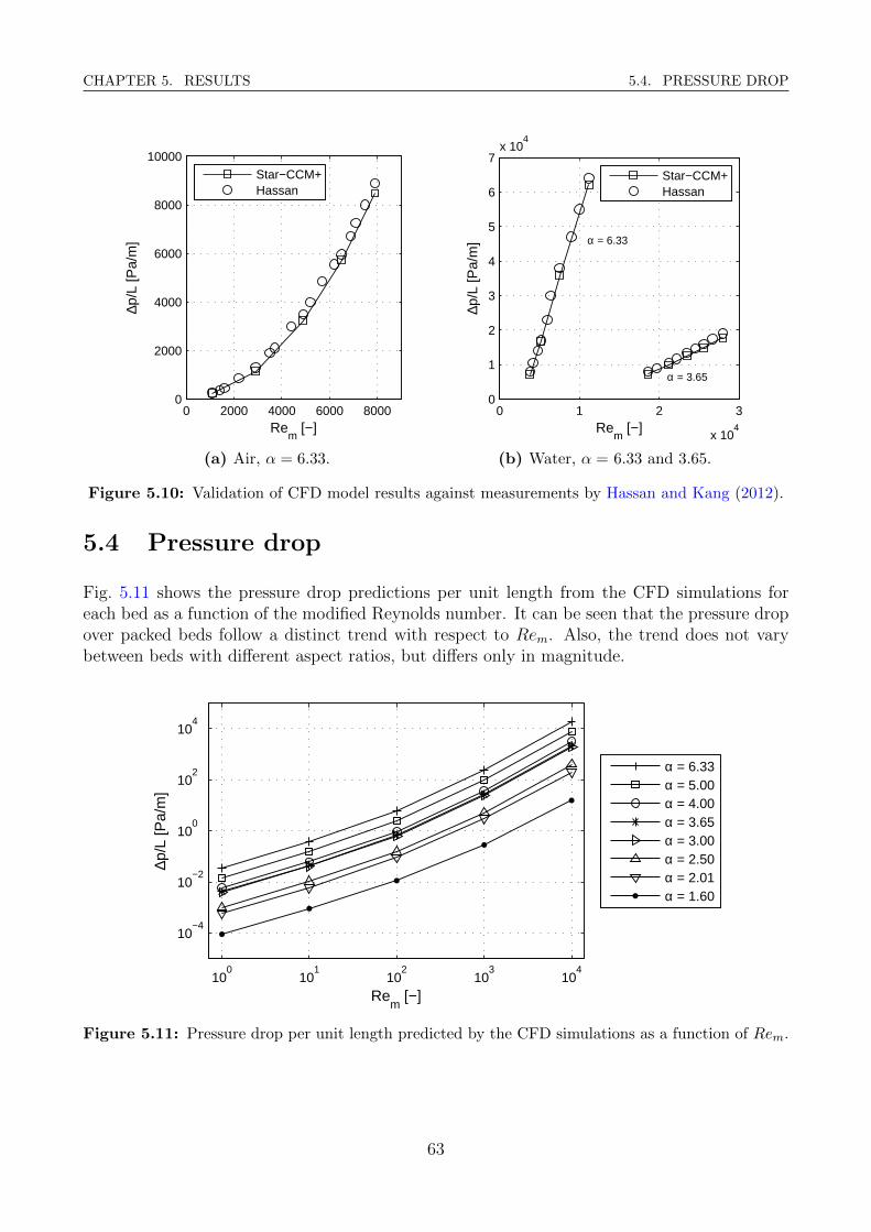
CHAPTER 5. RESULTS 5.4. PRESSURE DROP
0 2000 4000 6000 80000
2000
4000
6000
8000
10000
∆p/L
[Pa/
m]
Rem
[−]
Star−CCM+Hassan
(a) Air, α = 6.33.
0 1 2 3
x 104
0
1
2
3
4
5
6
7x 10
4
∆p/L
[Pa/
m]
Rem
[−]
α = 6.33
α = 3.65
Star−CCM+Hassan
(b) Water, α = 6.33 and 3.65.
Figure 5.10: Validation of CFD model results against measurements by Hassan and Kang (2012).
5.4 Pressure drop
Fig. 5.11 shows the pressure drop predictions per unit length from the CFD simulations foreach bed as a function of the modified Reynolds number. It can be seen that the pressure dropover packed beds follow a distinct trend with respect to Rem. Also, the trend does not varybetween beds with different aspect ratios, but differs only in magnitude.
100
101
102
103
104
10−4
10−2
100
102
104
∆p/L
[Pa/
m]
Rem
[−]
α = 6.33α = 5.00α = 4.00α = 3.65α = 3.00α = 2.50α = 2.01α = 1.60
Figure 5.11: Pressure drop per unit length predicted by the CFD simulations as a function of Rem.
63
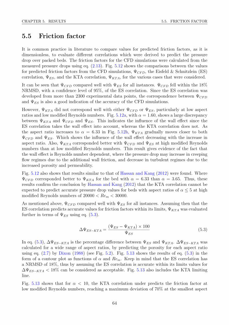
CHAPTER 5. RESULTS 5.5. FRICTION FACTOR
5.5 Friction factor
It is common practice in literature to compare values for predicted friction factors, as it isdimensionless, to evaluate different correlations which were derived to predict the pressuredrop over packed beds. The friction factors for the CFD simulations were calculated from themeasured pressure drops using eq. (2.13). Fig. 5.12 shows the comparisons between the valuesfor predicted friction factors from the CFD simulations, ΨCFD, the Eisfeld & Schnitzlein (ES)correlation, ΨES, and the KTA correlation, ΨKTA, for the various cases that were considered.
It can be seen that ΨCFD compared well with ΨES for all instances. ΨCFD fell within the 18%NRMSD, with a confidence level of 95%, of the ES correlation. Since the ES correlation wasdeveloped from more than 2300 experimental data points, the correspondence between ΨCFD
and ΨES is also a good indication of the accuracy of the CFD simulations.
However, ΨKTA did not correspond well with either ΨCFD or ΨES, particularly at low aspectratios and low modified Reynolds numbers. Fig. 5.12a, with α = 1.60, shows a large discrepancybetween ΨKTA and ΨCFD and ΨES. This indicates the influence of the wall effect since theES correlation takes the wall effect into account, whereas the KTA correlation does not. Asthe aspect ratio increases to α = 6.33 in Fig. 5.12h, ΨKTA gradually moves closer to bothΨCFD and ΨES. Which shows the influence of the wall effect decreasing with the increase inaspect ratio. Also, ΨKTA corresponded better with ΨCFD and ΨES at high modified Reynoldsnumbers than at low modified Reynolds numbers. This result gives evidence of the fact thatthe wall effect is Reynolds number dependent, where the pressure drop may increase in creepingflow regimes due to the additional wall friction, and decrease in turbulent regimes due to theincreased porosity and permeability.
Fig. 5.12 also shows that results similar to that of Hassan and Kang (2012) were found. WhereΨCFD corresponded better to ΨKTA for the bed with α = 6.33 than α = 3.65. Thus, theseresults confirm the conclusion by Hassan and Kang (2012) that the KTA correlation cannot beexpected to predict accurate pressure drop values for beds with aspect ratios of α ≤ 5 at highmodified Reynolds numbers of 20000 < Rem < 30000.
As mentioned above, ΨCFD compared well with ΨES for all instances. Assuming then that theES correlation predicts accurate values for friction factors within its limits, ΨKTA was evaluatedfurther in terms of ΨES using eq. (5.3).
∆ΨES−KTA =(ΨES −ΨKTA)× 100
ΨES
(5.3)
In eq. (5.3), ∆ΨES−KTA is the percentage difference between ΨES and ΨKTA. ∆ΨES−KTA wascalculated for a wide range of aspect ratios, by predicting the porosity for each aspect ratiousing eq. (2.7) by Dixon (1988) (see Fig. 5.2). Fig. 5.13 shows the results of eq. (5.3) in theform of a contour plot as functions of α and Rem. Keep in mind that the ES correlation hasa NRMSD of 18%, thus by assuming the ES correlation is accurate within its limits values for∆ΨES−KTA < 18% can be considered as acceptable. Fig. 5.13 also includes the KTA limitingline.
Fig. 5.13 shows that for α < 10, the KTA correlation under predicts the friction factor atlow modified Reynolds numbers, reaching a maximum deviation of 70% at the smallest aspect
64

CHAPTER 5. RESULTS 5.5. FRICTION FACTOR
100
101
102
103
104
100
101
102
103
Rem
[−]
Ψ [−
]
ESKTACFD
(a) α = 1.60.
100
101
102
103
104
100
101
102
103
Rem
[−]
Ψ [−
]
ESKTACFD
(b) α = 2.01.
100
101
102
103
104
100
101
102
103
Rem
[−]
Ψ [−
]
ESKTACFD
(c) α = 2.50.
100
101
102
103
104
100
101
102
103
Rem
[−]
Ψ [−
]
ESKTACFD
(d) α = 3.00.
100
101
102
103
104
100
101
102
103
Rem
[−]
Ψ [−
]
ESKTACFD
(e) α = 3.65.
100
101
102
103
104
100
101
102
103
Rem
[−]
Ψ [−
]
ESKTACFD
(f) α = 4.00.
100
101
102
103
104
100
101
102
103
Rem
[−]
Ψ [−
]
ESKTACFD
(g) α = 5.00.
100
101
102
103
104
100
101
102
103
Rem
[−]
Ψ [−
]
ESKTACFD
(h) α = 6.33.
Figure 5.12: Comparison of friction factors between ES, KTA and CFD simulations as a function ofRem.
65
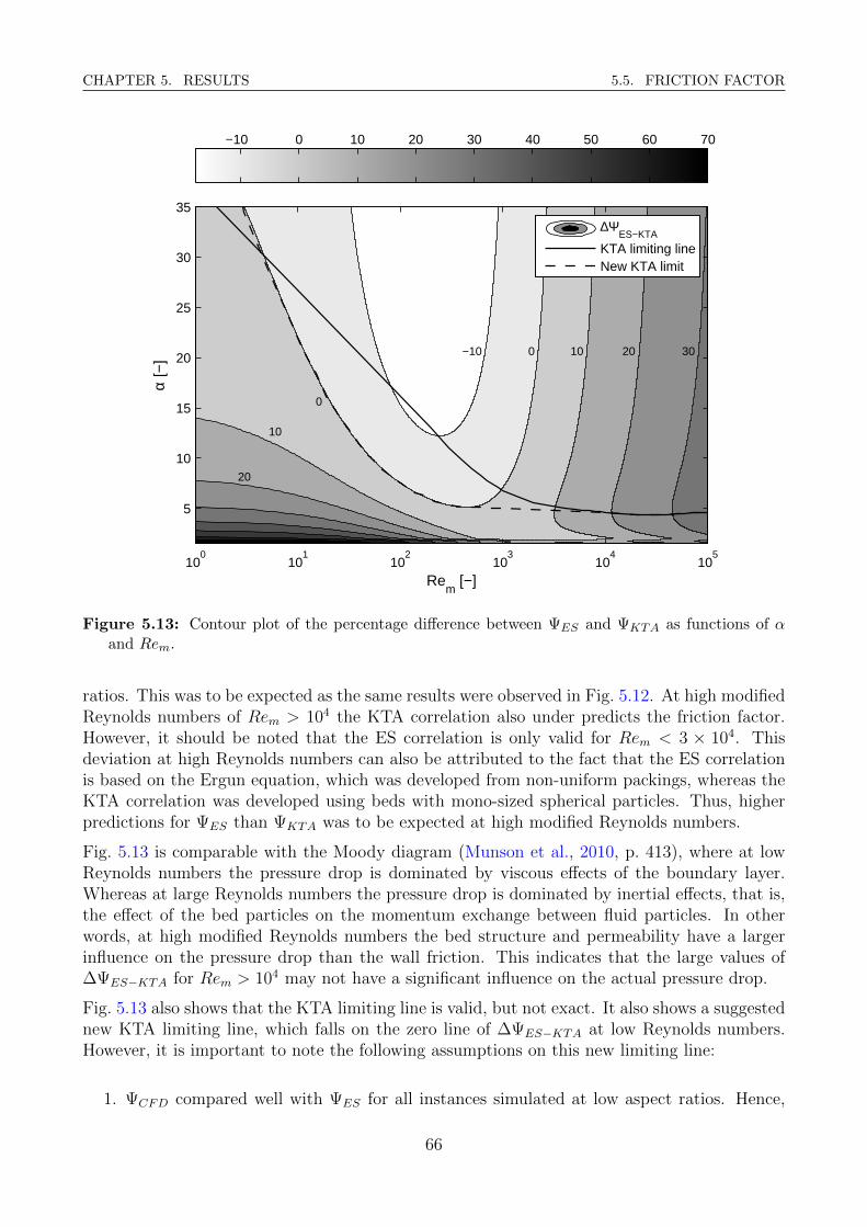
CHAPTER 5. RESULTS 5.5. FRICTION FACTOR
Rem
[−]
α [−
]
−10 0 10 20 30
0
10
20
100
101
102
103
104
105
5
10
15
20
25
30
35
−10 0 10 20 30 40 50 60 70
∆ΨES−KTA
KTA limiting lineNew KTA limit
Figure 5.13: Contour plot of the percentage difference between ΨES and ΨKTA as functions of αand Rem.
ratios. This was to be expected as the same results were observed in Fig. 5.12. At high modifiedReynolds numbers of Rem > 104 the KTA correlation also under predicts the friction factor.However, it should be noted that the ES correlation is only valid for Rem < 3 × 10⁴. Thisdeviation at high Reynolds numbers can also be attributed to the fact that the ES correlationis based on the Ergun equation, which was developed from non-uniform packings, whereas theKTA correlation was developed using beds with mono-sized spherical particles. Thus, higherpredictions for ΨES than ΨKTA was to be expected at high modified Reynolds numbers.
Fig. 5.13 is comparable with the Moody diagram (Munson et al., 2010, p. 413), where at lowReynolds numbers the pressure drop is dominated by viscous effects of the boundary layer.Whereas at large Reynolds numbers the pressure drop is dominated by inertial effects, that is,the effect of the bed particles on the momentum exchange between fluid particles. In otherwords, at high modified Reynolds numbers the bed structure and permeability have a largerinfluence on the pressure drop than the wall friction. This indicates that the large values of∆ΨES−KTA for Rem > 104 may not have a significant influence on the actual pressure drop.
Fig. 5.13 also shows that the KTA limiting line is valid, but not exact. It also shows a suggestednew KTA limiting line, which falls on the zero line of ∆ΨES−KTA at low Reynolds numbers.However, it is important to note the following assumptions on this new limiting line:
1. ΨCFD compared well with ΨES for all instances simulated at low aspect ratios. Hence,
66
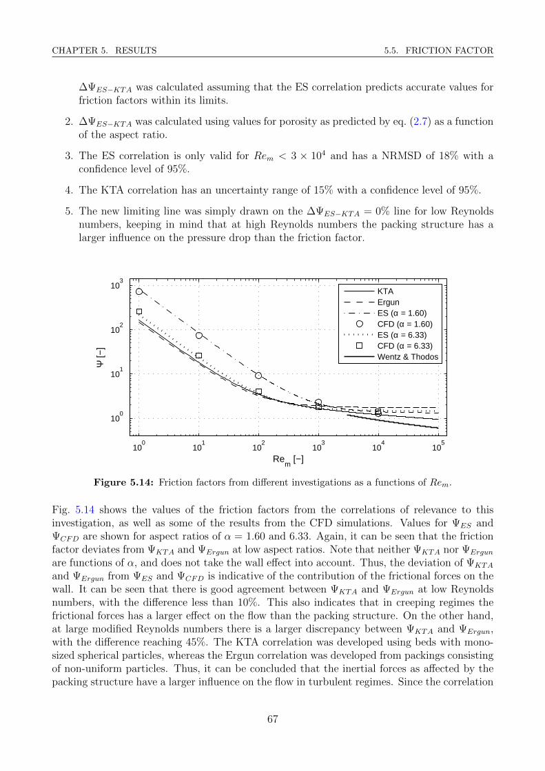
CHAPTER 5. RESULTS 5.5. FRICTION FACTOR
∆ΨES−KTA was calculated assuming that the ES correlation predicts accurate values forfriction factors within its limits.
2. ∆ΨES−KTA was calculated using values for porosity as predicted by eq. (2.7) as a functionof the aspect ratio.
3. The ES correlation is only valid for Rem < 3 × 10⁴ and has a NRMSD of 18% with aconfidence level of 95%.
4. The KTA correlation has an uncertainty range of 15% with a confidence level of 95%.
5. The new limiting line was simply drawn on the ∆ΨES−KTA = 0% line for low Reynoldsnumbers, keeping in mind that at high Reynolds numbers the packing structure has alarger influence on the pressure drop than the friction factor.
100
101
102
103
104
105
100
101
102
103
Ψ [−
]
Rem
[−]
KTAErgunES (α = 1.60)CFD (α = 1.60)ES (α = 6.33)CFD (α = 6.33)Wentz & Thodos
Figure 5.14: Friction factors from different investigations as a functions of Rem.
Fig. 5.14 shows the values of the friction factors from the correlations of relevance to thisinvestigation, as well as some of the results from the CFD simulations. Values for ΨES andΨCFD are shown for aspect ratios of α = 1.60 and 6.33. Again, it can be seen that the frictionfactor deviates from ΨKTA and ΨErgun at low aspect ratios. Note that neither ΨKTA nor ΨErgun
are functions of α, and does not take the wall effect into account. Thus, the deviation of ΨKTA
and ΨErgun from ΨES and ΨCFD is indicative of the contribution of the frictional forces on thewall. It can be seen that there is good agreement between ΨKTA and ΨErgun at low Reynoldsnumbers, with the difference less than 10%. This also indicates that in creeping regimes thefrictional forces has a larger effect on the flow than the packing structure. On the other hand,at large modified Reynolds numbers there is a larger discrepancy between ΨKTA and ΨErgun,with the difference reaching 45%. The KTA correlation was developed using beds with mono-sized spherical particles, whereas the Ergun correlation was developed from packings consistingof non-uniform particles. Thus, it can be concluded that the inertial forces as affected by thepacking structure have a larger influence on the flow in turbulent regimes. Since the correlation
67
CHAPTER 5. RESULTS 5.6. SUMMARY
by Wentz and Thodos, eq. (2.18), was derived from structured packings consisting of mono-sized spherical particles, the deviation of ΨWentz from ΨKTA and ΨErgun also reinforces thisconclusion. In future investigations, the effect of the inertial forces on the friction factor as afunction of the packing structure needs to be investigated in more detail.
5.6 Summary
This chapter contained the results from the CFD simulations of the flow through DEM gen-erated packed beds. All DEM and CFD simulations were run with the methods developed inChapter 4. It was shown that the randomly packed beds generated using DEM was of highquality, and the structures of these beds were analysed. Detail was given on the computationalresources available for this investigation, as well as its limitations on the CFD simulations. Themethodology developed in Chapter 4 was validated with measurements from the experimentalinvestigations by Wentz and Thodos (1963) and Hassan and Kang (2012). Good agreement wasfound between the CFD predictions for pressure drop, and the experimental measurements.
The results for Ψ from the CFD simulations were compared to the predictions of Ψ from theKTA and ES correlations. It was found that at small aspect ratios, the KTA correlation underpredicts the friction factor. The results also gave evidence of the fact that the wall effect isReynolds number dependent, where the pressure drop may increase in creeping flow regimes dueto the additional wall friction, and decrease in turbulent regimes due to the increased porosityand permeability. Since ΨES compared well with ΨCFD in all instances, an assumption wasmade that the ES correlation is valid within its limits. ΨKTA was then analysed over a widerange of Reynolds numbers and aspect ratios at the hand of ΨES. The KTA limiting line for theKTA correlation was found to be valid, but not exact, and a new limiting line was suggested.
The results presented in this chapter fulfilled the goal of the investigation, which was to deter-mine the validity of the KTA limiting line. The next chapter concludes the investigation withconclusions made from the results of the explicit CFD simulations, and recommendations forfuture work on the topic.
68

Chapter 6
Conclusions
The goal of this investigation was to determine the validity of the KTA limiting line shownin Fig. 1.1, which is the proposed lower limit of the KTA correlation. This was to be doneusing an explicit approach, by simulating the flow through DEM generated packed beds. Thischapter presents the conclusions made from the results of the explicit CFD simulation, as wellas recommendations for future work on the topic.
6.1 Conclusions
This investigation used the commercial CFD package STAR-CCM+ R© to explicitly analyse theflow through DEM generated packed beds, with small aspect ratios. STAR-CCM+ R© was usedfor both the generation of randomly packed beds using DEM, and the simulation of the flowthrough the beds using CFD.
Steps were taken to ensure accurate solutions with a reasonable degree of confidence. Themethods developed by Theron (2011) for creating DEM generated packed beds were improvedupon, and beds with aspect ratios of 1.6 ≤ α ≤ 25 were generated. The quality of these bedswere analysed by calculating the particle overlaps, the bulk porosities and the porosity variationsin the axial direction. The particle overlaps were found to be small, with do,max < 0.08% forall beds. The bulk porosities were calculated with an analytical method as well as a numericalmethod. The differences in bulk porosity between the two methods were small, with ∆εb < 0.1%for all beds. These calculated values for the bulk porosities also corresponded well with thevalues predicted by correlations from literature, as well as experimental measurements. Thus,the DEM generated beds were of high quality, though it was found that the lengths of the beds,with L/d ' 10, were insufficient to fully eliminate the length effect.
Methods were also developed with regards to the CFD simulation of the flow through the DEMgenerated beds, to ensure simulations which presented realistic results. Particular attention wasgiven to the mesh generation, turbulence modelling and boundary conditions. It was decided touse a polyhedral mesh with two prism layers. Particles were connected with a specific contactarea to increase the mesh quality. The Realisable k−ε turbulence model was used, and velocityprofiles for fully developed laminar and turbulent flows were specified at the inlet boundary.The methods developed were validated with experimental measurements from literature, for
69
CHAPTER 6. CONCLUSIONS 6.2. RECOMMENDATIONS
both structured and randomly packed beds. Good agreement was found between the predictedpressure drops from the CFD simulations and the pressure drop measurements of five differentexperiments. It could be concluded then that the CFD simulations, set up with the methodsdeveloped during this investigation, presented realistic results.
With the available resources and the high computational demand of these simulations, the flowthrough beds with aspect ratios of α = 1.60, 2.01, 2.50, 3.00, 3.65, 4.00, 5.00 and 6.33 weresimulated. The values for the friction factors from the CFD simulations were calculated fromthe predicted pressure drops, and compared with the values predicted by the ES and KTAcorrelations. It was found that ΨCFD corresponded well with ΨES for all instances, as it fellwithin the 18% NRMSD of the ES correlation. However, ΨKTA did not correspond well witheither ΨCFD or ΨES, particularly at low aspect ratios and low modified Reynolds numbers.This indicated the influence of the wall effect, since the ES correlation takes the wall effect intoaccount, whereas the KTA correlation does not. The Reynolds number dependence of the walleffect could also be seen, where in creeping flow regimes the bed friction has an overwhelmingeffect on the pressure drop, whereas in turbulent regimes the structure and permeability of thebed has the overwhelming influence. It was also observed that the influence of the wall effecton the flow decreased as the aspect ratio increased.
Since a good correlation was found between ΨCFD and ΨES, and assuming that the ES correla-tion is valid within its limits, the percentage difference between ΨES and ΨKTA was calculatedfor a wide range of α and Rem. It was found that the KTA limiting line is valid, but notexact. A new limiting line for the KTA correlation was suggested, however this new limitingline improved little on the existing line and was still the result of some major assumptions. Inorder to improve the determination of the position of the KTA limiting line further, criterianeed to be established which determine how small the error in predicted friction factor mustbe before the KTA correlation can be accepted as accurate. Further investigation is requiredto develop this criteria, as it must take into account the random nature of packed beds and theerrors of the ES and KTA correlations.
6.2 Recommendations
This investigation showed that simulating the flow through DEM generated packed beds ex-plicitly do present realistic results. However, these simulations are computationally intensive,and with more resources many improvements could be made to the investigation. The followingpoints are recommendations which could be used in future investigations which analyse the flowthrough packed beds using an explicit approach:
1. As mentioned above, this investigation showed that the KTA limiting line is valid, butnot exact. In order to improve the determination of the position of the KTA limiting line,criteria need to be established which determine how small the error in predicted frictionfactor must be before the KTA correlation can be accepted as accurate.
2. Future studies may include explicitly simulating the flow through packed beds at higheraspect ratios, if the appropriate resources are available.
3. With the analysis of the DEM generated beds used in this investigation, it was found that
70
CHAPTER 6. CONCLUSIONS 6.2. RECOMMENDATIONS
L/d ' 10 was insufficient to fully eliminate the length effect. Further analysis is requiredto determine the limit where the length effect can be considered negligible.
4. From the analysis of the DEM generated beds, it was found that the packing structuredepends heavily on the aspect ratio. Future work may include in depth analysis of thepacking structure as a function of the aspect ratio. With the particular goals of deter-mining the limits between structured and random packings, and quantifying phenomenasuch as the unusually long length effect observed in the bed with α = 3.00.
5. The methods developed in this investigation for the simulation of the flow through packedbeds were validated with experimental measurements from literature. Future work couldinclude building an in-house experimental setup with the specific goal of validating theCFD simulation results over a wide range of modified Reynolds numbers and aspect ratios.
6. This investigation focussed only on the pressure drop over packed beds, thus the controlvolumes were considered adiabatic and no heat transfer was modelled. Future studiesmay include modelling the heat transfer between the fluid and the particles. Particularlywith a heat source within the particles, as is the case in nuclear packed bed reactors.
7. The particles were connected with a specific contact area to increase the mesh quality.The size of the contact area was of little importance in the current investigation, as longas it did not influence the pressure drop over the bed. If in future work the heat transferbetween particles were to be modelled, particular focus would need to be given to the sizeof the contact area and the effective conduction heat transfer coefficient between particles.
8. Localised recovery of total pressure was observed in the flow between particles, at theexpense of depletion of total pressure elsewhere in the domain. The potential influencethat local total pressure rises may have on the heat transfer within packed beds shouldalso be investigated.
9. It was found that the packing structure has a large influence on the flow through packedbeds. In future investigations the effect of the inertial forces on the friction factor as afunction of the packing structure needs to be investigated in more detail.
71
Bibliography
Bai, H., Theuerkauf, J., Gillis, P.A., and Witt, P.M. (2009). A coupled DEM and CFD sim-ulation of flow field and pressure drop in fixed bed reactor with randomly packed catalystparticles. Industrial and Engineering Chemistry Research, 48(8):4060–4074.
Benenati, R.F. and Brosilow, C.B. (1962). Void fraction distribution in beds of spheres. AIChEJournal, 8(3):359–361.
Benyahia, F. and O’Neill, K.E. (2005). Enhanced voidage correlations for packed beds of variousparticle shapes and sizes. Particulate Science and Technology, 23(2):169–177.
Blake, F.C. (1922). The resistance of packing to fluid flow. Transactions of the Institution ofChemical Engineers, 14:415–421.
Calis, H.P.A., Nijenhuis, J., Paikert, B.C., Dautzenberg, F.M., and Van den Bleek, C.M. (2001).CFD modelling and experimental validation of pressure drop and flow profile in a novelstructured catalytic reactor packing. Chemical Engineering Science, 56(4):1713–1720.
Carman, P. (1937). Fluid flow through granular beds. Transactions of the Institution of Chem-ical Engineers, 15:150–166.
CD-Adapco (2012). STAR-CCM+ User guide. 7th edition.
Cheng, G. and Yu, A. (2013). Particle scale evaluation of the effective thermal conductivityfrom the structure of a packed bed: Radiation heat transfer. Industrial and EngineeringChemistry Research, 52(34):12202–12211.
Cheng, G., Yu, A., and Zulli, P. (1999). Evaluation of effective thermal conductivity from thestructure of a packed bed. Chemical Engineering Science, 54(19):4199 – 4209.
Cheng, N. (2011). Wall effect on pressure drop in packed beds. Powder Technology, 210(3):261–266.
Cohen, Y. and Metzner, A.B. (1981). Wall effects in laminar flow of fluids through packed beds.AICHE J., 27(4):705–715.
Cundall, P.A. and Strack, O.D.L. (1979). Discrete numerical model for granular assemblies.Geotechnique, 29(1):47–65.
De Klerk, A. (2003). Voidage variation in packed beds at small column to particle diameterratio. AIChE Journal, 49(8):2022–2029.
72
BIBLIOGRAPHY
Di Felice, R. and Gibilaro, L.G. (2004). Wall effects for the pressure drop in fixed beds. ChemicalEngineering Science, 59(14):3037–3040.
Dixon, A.G. (1988). Correlations for wall and particle shape effects on fixed bed bulk voidage.Canadian Journal of Chemical Engineering, 66(5):705–708.
Dixon, A.G., Nijemeisland, M., and Stitt, E.H. (2013). Systematic mesh development for 3DCFD simulation of fixed beds: Contact points study. Computers & Chemical Engineering,48:135–153.
Dolejs, V. and Machac, I. (1995). Pressure drop during the flow of a newtonian fluid through afixed bed of particles. Chemical Engineering & Processing: Process Intensification, 34(1):1–8.
Du Toit, C.G. (2008). Radial variation in porosity in annular packed beds. Nuclear Engineeringand Design, 238(11):3073–3079.
Du Toit, C.G. and Rosslee, P.J. (2012). Analysis of the porous structure of packed beds ofspheres using x-ray computed tomography. In Eighth South African conference on computa-tional and applied mechanics, SACAM.
Du Toit, C.G., Van Antwerpen, W., and Rousseau, P.G. (2009). Analysis of the porous structureof an annular pebble bed reactor. In ICAPP, 9123.
Eisfeld, B. and Schnitzlein, K. (2001). The influence of confining walls on the pressure drop inpacked beds. Chemical Engineering Science, 56(14):4321–4329.
Eppinger, T., Seidler, K., and Kraume, M. (2011). DEM-CFD simulations of fixed bed reactorswith small tube to particle diameter ratios. Chemical Engineering Journal, 166(1):324–331.
Ergun, S. (1952). Fluid flow through packed columns. Chemical Engineering Progress, 48(2):89–94.
Goodling, J.S., Vachon, R.I., Stelpflug, W.S., Ying, S.J., and Khader, M.S. (1983). Radialporosity distribution in cylindrical beds packed with spheres. Powder Technology, 35(1):23–29.
Graton, L.C. and Fraser, H.J. (1935). Systematic packing of spheres: With particular relationto porosity and permeability. The Journal of Geology, 43(8):785–909.
Hassan, Y.A. (2008). Large eddy simulation in pebble bed gas cooled core reactors. NuclearEngineering and Design, 238(3):530–537.
Hassan, Y.A. and Kang, C. (2012). Pressure drop in a pebble bed reactor under high Reynoldsnumber. Nuclear Technology, 180(2):159–173.
Issa, R.I. (1995). Rise of total pressure in frictional flow. AIAA journal, 33(4):772–774.
KTA (1981). Reactor core design of high-temperature gas-cooled reactors. Part 3: Loss ofpressure through friction in pebble bed cores. Nuclear Safety Standards Commission, “Kern-technischer Ausschuss”, 3102.3:1–4.
73
BIBLIOGRAPHY
KTA (1988). Safety Standard by the Nuclear Safety Standards Commission, “KerntechnischerAusschuss”. “Bundesanzeiger”, 44:D1–D36.
Lee, J.J., Park, G.C., Kim, K.Y., and Lee, W.J. (2007). Numerical treatment of pebble contactin the flow and heat transfer analysis of a pebble bed reactor core. Nuclear Engineering andDesign, 237(22):2183–2196.
Leva, M. and Grummer, M. (1947). Pressure drop through packed tubes, Part III Predictionof voids in packed tubes. Chemical Engineering Progress, 43(12):713–718.
Mariani, N.J., Salvat, W.I., Campesi, A., Barreto, G.F., and Martinez, O.M. (2009). Eval-uation of structural properties of cylindrical packed beds using numerical simulations andtomographic experiments. International Journal of Chemical Reactor Engineering, 7:1.
Mehta, D. and Hawley, M.C. (1969). Wall effect in packed columns. Industrial and EngineeringChemistry Design and Development, 8(2):280–282.
Mueller, G.E. (1992). Radial void fraction distributions in randomly packed fixed beds of uni-formly sized spheres in cylindrical containers. Powder Technology, 72(3):269–275.
Mueller, G.E. (1997). Angular porosity distributions in fixed packed beds of low diameter aspectratio. Canadian Journal of Chemical Engineering, 75(4):677–683.
Mueller, G.E. (2010). Radial porosity in packed beds of spheres. Powder Technology, 203(3):626–633.
Mueller, G.E. (2012). A simple method for determining sphere packed bed radial porosity.Powder Technology, 229:90–96.
Munson, B.R., Young, D.F., Okiishi, T.H., and Huebsch, W.W. (2010). Fundamentals of fluidmechanics. John Wiley and Sons, Inc., 6th edition.
Preller, A.C.N. (2011). Numerical modelling of flow through packed beds of uniform spheres.Master of engineering in nuclear engineering, North-West University.
Reddy, R.K. and Joshi, J.B. (2008). CFD modeling of pressure drop and drag coefficient infixed and expanded beds. Chemical Engineering Research and Design, 86(5):444–453.
Reddy, R.K. and Joshi, J.B. (2010). CFD modeling of pressure drop and drag coefficient infixed beds: Wall effects. Particuology, 8(1):37–43.
Reichelt, W. (1972). Calculation of pressure drop in spherical and cylindrical packings forsingle-phase flow (Zur Berechnung des Druckverlustes einphasig durchstroemter Kugel- undZylinderschuettungen). Chemie-Ingenieur-Technik, 44(18):1068–1071.
Reyneke, H.J. (2009). Investigation into the velocity distribution through an annular packed bed.Master of engineering in nuclear engineering, North-West University.
Reynolds, O. (1900). Papers on mechanical and physical subjects. Cambridge University Press,14:81–85.
74

BIBLIOGRAPHY
Ridgway, K. and Tarbuck, K.J. (1966). Radial voidage variation in randomly-packed beds ofspheres of different sizes. Journal of Pharmacy and Pharmacology, 18(S1):168S–175S.
Roblee, L.H.S., Baird, R.M., and Tierney, J.W. (1958). Radial porosity variations in packedbeds. AIChE Journal, 4(4):460–464.
Rosslee, P.J. (2009). Analysis of the variation in the porosity of packed columns. Technicalreport, North-West University, Potchefstroom, South-Africa.
Sederman, A.J., Alexander, P., and Gladden, L.F. (2001). Structure of packed beds probed bymagnetic resonance imaging. Powder Technology, 117(3):255–269.
Tabor, G.R. and Baba-Ahmadi, M.H. (2010). Inlet conditions for large eddy simulation: Areview. Computers and Fluids, 39(4):553–567.
Theron, W.G.J. (2011). Numerical analysis of the flow distribution within packed columns usingan explicit approach. Master of engineering in nuclear engineering, North-West University.
Van Antwerpen, W., Du Toit, C.G., and Rousseau, P.G. (2010). A review of correlations tomodel the packing structure and effective thermal conductivity in packed beds of mono-sizedspherical particles. Nuclear Engineering and Design, 240(7):1803–1818.
Versteeg, H.K. and Malalasekera, W. (2007). An introduction to Computational Fluid Dynam-ics: The finite volume method. Pearson Education Limited, 2nd edition.
Voronoi, M.G. (1908). Nouvelles applications des parametres continus a la theorie des formesquadratiques. Deuxieme memoire. Recherches sur les parallelloedres primitifs. Journal furdie reine und angewandte Mathematik, 134:198–287.
Wensrich, C. (2012). Boundary structure in dense random packing of monosize spherical par-ticles. Powder Technology, 219:118–127.
Wentz, C.A. and Thodos, G. (1963). Pressure drops in the flow of gases through packed anddistended beds of spherical particles. AIChE Journal, 9(1):81–84.
White, S.M. and Tien, C.L. (1987). Analysis of flow channeling near the wall in packed beds.Warme - und Stoffubertragung, 21:291–296.
Winterberg, M. and Tsotsas, E. (2000). Impact of tube-to-particle-diameter ratio on pressuredrop in packed beds. AIChE Journal, 46:1084–1088.
Zhu, H.P., Zhou, Z.Y., Yang, R.Y., and Yu, A.B. (2007). Discrete particle simulation of partic-ulate systems: Theoretical developments. Chemical Engineering Science, 62(13):3378–3396.
Zou, R.P. and Yu, A.B. (1995). The packing of spheres in a cylindrical container: the thicknesseffect. Chemical Engineering Science, 50(9):1504–1507.
75

LATEX