analysis of floating support structures for marine …
TRANSCRIPT
ANALYSIS OF FLOATING SUPPORT STRUCTURES FOR MARINE
AND WIND ENERGY
A thesis submitted to the University of Manchester towards the degree of
Doctor of Philosophy (PhD)
In the Faculty of Engineering and Physical Sciences
2014
Emmanuel Fernandez Rodriguez
School of Mechanical, Aerospace and Civil Engineering

2
List of Contents
List of Symbols ............................................................................................................. 5
List of Figures ............................................................................................................. 12
List of Tables .............................................................................................................. 16
Abstract ...................................................................................................................... 17
Declaration ................................................................................................................. 18
Copyright.................................................................................................................... 19
Acknowledgements ..................................................................................................... 20
CHAPTER 1: INTRODUCTION ................................................................................ 21
1.1 Tidal Stream Background ...................................................................................... 21
1.2 Tidal Energy Resource .......................................................................................... 21
1.3 Support Structures for Offshore Turbines .............................................................. 22
1.4 Design of Floating Platforms ................................................................................. 23
1.5 Objectives ............................................................................................................. 23
1.6 Structure of Thesis ................................................................................................ 24
CHAPTER 2: HORIZONTAL-AXIS TURBINE MODELLING ................................ 26
2.1 Tidal Streams ........................................................................................................ 26
2.2 Flow Conditions at Tidal Stream Sites ................................................................... 27
2.3 Modelling Methods for Individual Turbines .......................................................... 29
2.4 Studies of Rotors in Uniform and Sheared Flows .................................................. 30
2.5 Blade Element Momentum Theory ........................................................................ 32
2.6 Linear Momentum Theory .................................................................................... 33
2.7 Blade Element Theory ........................................................................................... 36
2.8 Blade Element Momentum Theory ........................................................................ 38
2.9 High axial Induction Factor ................................................................................... 40
2.10 Blockage Correction ............................................................................................ 42

3
2.11 Iterative Solution to Obtain Axial and Radial Induction Factors .......................... 43
2.12 Unsteady Incident Flows ..................................................................................... 44
2.13 Extreme-Value Analysis ...................................................................................... 49
2.14 Conclusions......................................................................................................... 54
CHAPTER 3: LOADING OF A TIDAL STREAM TURBINE IN TURBULENT
CHANNEL FLOW ..................................................................................................... 55
3.1 BEM Model Predictions ........................................................................................ 55
3.2 Mean Thrust and Power in Turbulent Channel Flow .............................................. 58
3.3 Variance of Rotor Thrust ....................................................................................... 63
3.4 Peak Thrust in Turbulent Channel Flow Only ........................................................ 65
3.5 Extreme-Value Distribution .................................................................................. 69
3.6 Conclusions .......................................................................................................... 71
CHAPTER 4: LOADING OF OSCILLATING POROUS DISCS AND ROTORS...... 72
4.1 Introduction .......................................................................................................... 72
4.2 Review of Hydrodynamics of Oscillating Porous Discs in Still Water ................... 76
4.3 Comparison of Forced Oscillation of Rotors and Discs in Uniform Flow ............... 78
4.4 Experimental Arrangement ................................................................................... 80
4.5 Drag and Damping of Oscillating Porous Discs in Still Water ............................... 82
4.6 Drag and Damping of Oscillating Porous Discs and Rotors in Turbulent Flow ...... 85
4.7 Extreme loads on Oscillating Rotors in Turbulent Channel Flow ........................... 90
4.8 Summary............................................................................................................... 94
CHAPTER 5: LOADING DUE TO WAVES COMBINED WITH TURBULENT
CHANNEL FLOW ..................................................................................................... 96
5.1 Introduction .......................................................................................................... 96
5.2 Experimental Measurement ................................................................................... 96
5.3 Variation of Extreme Loads with Wave Height ..................................................... 97
5.4 Extreme Loads due to Turbulent Channel Flow with Waves: Drag Prediction ..... 100

4
5.5 Time-varying Kinematics and Drag due to Waves and Turbulence ...................... 103
5.6 Prediction of Extreme Loads based on Forced Streamwise Oscillations of the Rotor
in a Turbulent Channel Flow ..................................................................................... 106
5.7 Summary............................................................................................................. 108
CHAPTER 6: SUPPORT-STRUCTURE DYNAMICS ............................................. 109
6.1 Introduction ........................................................................................................ 109
6.2 Support Structures for Horizontal-Axis Wind and Tidal Stream Turbines at Shallow
and Intermediate Water Depths ................................................................................. 110
6.3 Floating Support Structures for Horizontal-Axis Turbines ................................... 113
6.4 Floating Platform Dynamic Models ..................................................................... 117
6.5 Hydrostatic and Hydrodynamic Coefficients of Floating Support Structures ........ 121
6.6 Wave Induced Forces and Moments .................................................................... 122
6.7 External Forcing.................................................................................................. 125
6.8 Damping and Added mass ................................................................................... 126
6.9 Single Mode Response: Surge Only .................................................................... 128
6.10 Coupled Pitch and Surge ................................................................................... 136
6.11 Summary ........................................................................................................... 138
CHAPTER 7: CONCLUSIONS ................................................................................ 140
References ................................................................................................................ 149
Appendix A .............................................................................................................. 163
Appendix B............................................................................................................... 168
Appendix C .............................................................................................................. 169
Words count 45,764
5
List of Symbol
aaxial Axial induction factor
𝑎 Added mass of a disc
aT Tangential induction factor
ac High axial induction threshold
𝐴 Swept area
𝐴D Area of the disc
𝐴w Area of the downstream
𝐴wave Wave amplitude
𝐴0 Area of the upstream tube
𝑎i,j Added mass of the support structure in the six coupled modes
𝑎k,i,j Ratio of added mass between the platform and supported rotors in
the six coupled modes
𝑏 Damping of disc
𝑏i,j Damping of support structure in the six coupled modes
𝑏k,i,j Damping between support structure and rotor
𝑏max,i,j Maximum disc damping in the six coupled modes
𝑏ord Ordinate
𝐵 Number of blades
𝑐 Chord
𝑐i,j Restoring coefficient of the support in the six coupled modes
𝐶a Added mass coefficient
𝐶′a,i,j Added mass coefficient of the rotor expressed with volume of a disc
for the six coupled modes
𝐶b Damping coefficient of rotor in surge
𝐶d Foil drag coefficient
𝐶D Oscillatory drag coefficient
𝐶D,c Drag coefficient in uniform flow
𝐶D,1 Drag coefficient in combined current and oscillatory flow due to
contribution of the current velocity only

6
𝐶D,2 Drag coefficient in combined current and oscillatory flow due to
contribution of the oscillatory velocity
𝐶D,wave Drag coefficient in combined current and waves due to contribution
of wave velocity
𝐶i Temporal correlation factor
𝐶l Foil lift coefficient
𝐶M Inertia coefficient
𝐶P Power coefficient
𝐶P,max Betz limit
𝐶T Thrust coefficient
𝐶x Horizontal force of blade section
𝐶y In-plane force of blade section
𝐷 Diameter
𝐷l Length Characteristic
𝐸 Energy spectrum of the incident flow
finitial Initial conditions
fH Local hub loss multiplying factor
fk Local tip loss multiplying factor
𝑓 Frequency
𝑓n Natural frequency
𝑓r Frequency of mean rotational speed
𝑓wave Peak frequency of wave
𝐹 Force
�̅� Mean force of the combined oscillatory and turbulent flow
𝐹′ Force fluctuations around the mean
𝐹drag Drag force on the blade segment
𝐹dynamic Dynamic force
𝐹D,1 Drag force in oscillatory flow due to current flow separation
𝐹D,2 Drag force in oscillatory flow due to streamwise velocity separation
𝐹H Hub loss factor
𝐹j Individual force from time-varying measurements
𝐹k Tip loss factor

7
𝐹l Lift force
𝐹loss Tip and hub losses factor
𝐹m Measured force
𝐹mech,t Force to overcome the mechanical friction and tower
𝐹neglected,1 Neglected term in the Morison equation due to flow separation of
the current
𝐹neglected,2 Neglected term in the Morison equation due to flow separation of
the streamwise velocity
𝐹N Normal Rotor force
𝐹osc Rotor force due to imposed steady oscillations or waves
𝐹osc,max Maximum force due to oscillatory flow only
𝐹T Total force on the fluid
𝐹Th Threshold force
𝐹tower Tower load
𝐹turb Excitation force of the rotor in turbulent current
𝐹x Horizontal load
𝐹0 Time-averaged force in mean flow with turbulence present
𝐹1n Force with a probability of occurrence of 1
n
𝐹′1n Force with a probability of occurrence of 1
n due to the turbulent
fluctuations
𝑔 Gravity constant (9.81 m/s2)
ℎ Water depth of the wave-current flume
𝐻 Wave height
𝐻0 Mean wave height
𝐻s Significant wave height
𝑘 Wave number
𝑘i,j Stiffness of mooring lines
𝑘s Shape factor
k − 𝜖, k − ω Turbulence models
Kspera Spera thrust factor
𝐾𝐶 Keulegan Carpenter number
Ki Force factor in the six modes
8
𝐾I Admittance factor
lx Semi-axis length in x direction
ly Semi-axis length in y direction
lz Semi-axis length in z direction
𝐿 Length of the tower
𝐿ii Average length scale where 𝑖 = 𝑥, 𝑦, 𝑧
𝐿w Wave length
𝑚 Mass
𝑚rotor,i,j Mass of the rotor in the six coupled modes
𝑚slope Slope
𝑀 Time length of the long run measurement
𝑀a Mass of a spheroid
𝑀k,i,j Mass ratio in the six coupled modes
𝑚i,j Mass of the support structure in the six coupled modes
M2 Harmonics due to moon
𝑛exc Arbitrary number of measured forces
n Number of rotors
𝑁 Number of forces samples
𝑝 Pressure
𝑝0 Pressure at the upstream tube
𝑝4 Pressure at the wake
𝑝+ Pressure before the disc
𝑝− Pressure after the disc
P Probability
𝑃p Power
𝑄 Torque
𝑟 Radii
rms Root mean square
𝑟R Local radii over rotor radius
𝑅 Radius
R2res Least square residuals
𝑅hub Hub radius

9
𝑅𝑒 Reynolds number
S2 Harmonics due to sun
𝑡 Time
𝑡th Thickness
𝑇 Thrust
𝑇amb Period of the ambient flow based on energy spectrum of speed
fluctuations
𝑇𝐼 Turbulence Intensity
𝑇p Mean period of probability range
𝑇R Return period
𝑇wave The wave period
𝑇𝑆𝑅 Tip-Speed Ratio
𝑇𝑆𝑅r Local Tip-Speed Ratio
𝑢 Velocity of the ambient flow
𝑢′ Time fluctuations of the upstream velocity around the mean
𝑢b Bypass velocity
𝑢c Velocity in a mean flow with turbulence present
𝑢D Disc velocity
𝑢Dc Disc velocity in bounded flow
𝑢wave Wave velocity
𝑢wave,m Measured wave velocity
𝑢wave,p Wave velocity using linear wave theory
𝑢x Velocity in x-axis
𝑢w Wake velocity
𝑢wc Wake velocity in bounded flow
𝑢y Velocity in y-axis
𝑢z Velocity in z-axis
𝑢0 Mean upstream velocity
𝑢0c Equivalent water velocity to bounded flow
𝑈 Velocity at an arbitrary location of the stream tube
𝑈a Velocity of the incident flow using the Morison Equation
𝑈0 Depth-averaged velocity

10
𝑉 Volume
𝑥 Displacement in surge
𝑥i,j Motion of the support in the six coupled modes
‖�̇�‖max Highest measured amplitude of the forced rotor’s streamwise tests
𝑥rotor,i,j Motion of the rotor in the six coupled modes
𝑋 Matrix of set of differential equations
𝑋e,i External forcing in the six degrees of freedom
𝑋i Wave force in the six modes
𝑋h,i,j Hydrodynamics of support structure in the six coupled modes
𝜒2|𝑓| Admittance factor
𝑦 Vertical displacement
W Width
𝑊rel Relative wind velocity
𝑧 Distance along the flume depth
ℱnormal Normal distribution
ℱPareto Pareto distribution
ℱType 1 Type 1 distribution
ℱweibull Weibull distribution
𝛼 Angle of attack
𝛽 Stokes or Frequency number
𝛿 Phase
𝜂 Surface elevation
𝜀 Blockage factor
ξ Attenuation damping rate
𝛾 Blade-pitch angle
𝜆s Shape parameter
𝜇0 Mean of distribution
𝜇 Dynamic viscosity of medium
𝜈 Kinematic viscosity
𝜔 Angular speed
𝜑 Relative wind angle
𝜌 Density of fluid

11
𝜎 Standard deviation
𝜎r,a Alternative blade chord solidity
𝜎r Blade chord solidity
𝜏 Porosity ratio
𝜏t Correlation time
𝜃r Pitch response at the hub height

12
List of Figures
Figure 2.1 Wave scatter diagram for a tidal stream site in the Orkney Isles ................. 29
Figure 2.2 Actuator disc modified from Burton et al. (2001). Mass flow rate (𝜌𝐴𝑈) has to
be equal for all locations, hence the ...................................................................... 34
Figure 2.3 Forces and velocities obtained in a section of the blade. a) Diagram of the
velocities and the angles obtained ........................................................................ 36
Figure 3.1 Thrust and power predictions compared to published measurements (○) for a
pitch angle of 𝛾 = 5˚ ............................................................................................ 56
Figure 3.2 Thrust and power predictions compared to published measurements .......... 57
Figure 3.3 Power curve predictions for a single rotor using set of lift and drag coefficients
obtained ............................................................................................................... 58
Figure 3.4 Characteristics of the turbulent currents in the streamwise direction for a
porous plate at the inflow plane............................................................................ 60
Figure 3.5 Spectrum of the operating flow with an average 𝑇𝐼 =12% (-) and 𝑇𝐼 =14%
(--) obtained at the hub height from a single minute measurement. ....................... 61
Figure 3.6 Numerical model compared to the predicted thrust coefficient’s curve (Whelan
and Stallard, 2011) and 1-minute average measurements ...................................... 62
Figure 3.7 BEM predictions against published predictions (Whelan and Stallard, 2011)
without blockage and average of 1-minute ........................................................... 63
Figure 3.8 Statistical analysis of the measured and exceeded rotor forces. a) Histogram of
the forces greater than threshold force of 1 ........................................................... 66
Figure 3.9 Statistical analysis of the exceedance rotor forces in a mean flow with 𝑇𝐼 =
12%. .................................................................................................................... 67
Figure 3.10 Percentage difference of the 1% (left) and 0.1% (right) loads obtained with
different threshold forces and sample lengths ....................................................... 68
Figure 3.11 Probability plot for turbulent channel flow only........................................ 68
Figure 3.12 Probability force plots of three extreme methods in turbulent current with a
𝑇𝐼 =12% using a threshold force of 1.1 times ...................................................... 69
Figure 3.13 Comparison of the exceedance forces obtained using different extreme-value
methods ............................................................................................................... 70
Figure 4.1 Scale model of a spar truss platform ........................................................... 77
Figure 4.2 Diagram of the driving support structure. ................................................... 81

13
Figure 4.3 Excitation force of disc due to sinusoidal axial ........................................... 82
Figure 4.4 Variation of added mass (left) and damping coefficients (right) against 𝐾𝐶 for
a disc of porosity ratio 0.52 at different 𝛽 numbers. ............................................. 83
Figure 4.5 Measurements compared to the average trend of the linear (--) and Morison
drag coefficient (─) .............................................................................................. 84
Figure 4.6 Inertia coefficient in the quiescent flow using Eq. 2.39 and Eq. 2.44 with 𝐾𝐶
parameter and different 𝛽 numbers. Markers for 𝛽 number are as shown in Figure
4.4. ...................................................................................................................... 85
Figure 4.7 The oscillatory drag coefficients obtained in the quiescent and mean flow
conditions with turbulence against 𝐾𝐶 number .................................................... 88
Figure 4.8 Mean thrust coefficient against velocity ratio for disc and rotor. Predictions
using Eq. 4.16 (─). Markers of measurements as Figure 4.7. ................................ 92
Figure 4.9 Predictions of the exceedance loads 1% (--), 0.1% (--) and 0.01 % (--) using
an oscillatory drag coefficient of 2 against measurements .................................... 93
Figure 5.1 Experimental arrangement for the sea states conditions. Waves are generated
at the right opposing the turbulent current flow .................................................... 97
Figure 5.2 Difference in percentage of the 1% (left) and 0.1% (right) loads obtained with
different threshold forces and sample lengths ....................................................... 98
Figure 5.3 Force spectra for flow conditions without waves (-) and with waves of low
(--) and high amplitude of elevation (--). .............................................................. 99
Figure 5.4 The extreme load variation from the measured time-varying force compared
with the statistics of the surface elevations ......................................................... 100
Figure 5.5 Comparison of the measured and predicted amplitude of wave velocity at the
hub height (■) using linear wave theory ............................................................. 102
Figure 5.6 The measured exceedance forces in waves with probabilities of 1% (■), 0.1%
(▲) and 0.01% (i) and same forces .................................................................. 103
Figure 5.7 Time-varying force due to waves against predictions employing linear wave
kinematics at the hub height. --, predictions;─, measurements. ........................... 105
Figure 5.8 The oscillatory drag (X) of a rotor on a fixed support structure in turbulent
channel flow with opposing waves. 𝐾𝐶 .............................................................. 106
Figure 5.9 Predictions for the 1% (--), 0.1% (--) and 0.01% (--) wave forces using an
oscillatory drag coefficient of 2 .......................................................................... 107

14
Figure 6.1 Different concepts of support structures for wind turbines deployed at shallow
water depths. Source from Musial and Ram (2010). ........................................... 111
Figure 6.2 Concepts and illustrations of fixed supported configurations a) Marine Current
Turbine (MCT Ltd) ............................................................................................ 112
Figure 6.3 Demonstration systems for deep-water regions. Different floating structures
denoting a 1) semi-submersible type .................................................................. 113
Figure 6.4 Floating offshore turbines configurations for wind turbines at deep waters a)
Deployment of Hywind spar buoy turbine (Sun et al., 2012). ............................. 115
Figure 6.5 Scheme of the forces modelled from the floating system for six-degree freedom
of motion. .......................................................................................................... 118
Figure 6.6 Idealised platform supporting two rotors. Concept analogous to the Bluetec
(Van der Plas, 2014) and ScotRenewables ......................................................... 120
Figure 6.7 Half section of the immersed cylindrical body with hemispherical ends. .. 122
Figure 6.8 Forcing of the semi-submersible ............................................................... 124
Figure 6.9 a) Ratio of surge force, 𝑋1/𝐹D,max and b) pitch moment, 𝑋5/𝐿𝐹D,max, on
the support relative to the surface elevation ........................................................ 125
Figure 6.10 Ratio of hydrodynamic coefficients between the semi-submersible structure
and the rotor for modes corresponding ............................................................... 127
Figure 6.11 Dynamic force exerted on the mooring lines normalised to its mean using a
mass ratio of 1.5, K1=0.15 ................................................................................. 131
Figure 6.12 Linear displacement in a support unconstrained to surge using representative
damping, mass and force ratios .......................................................................... 132
Figure 6.13 Extreme forces with 1% probability of exceedance on one rotor supported
from a floating structure relative to same forces ................................................. 133
Figure 6.14 Extreme forces with 1% probability of exceedance on one of two rotors
supported from a floating structure..................................................................... 134
Figure 6.15 Extreme forces with 1% probability of exceedance on one rotor supported
from a floating structure ..................................................................................... 134
Figure 6.16 Extreme forces with 1% probability of exceedance on one of two rotors
supported from a floating structure..................................................................... 135
Figure 6.17 a) Force between a floating (--) and rigid-bed-connected support structure
(-) without turbulence ........................................................................................ 137

15
Figure A.1 Diagram of the Actuator Disc in a bounded flow. Linear Momentum is used
to calculate the total axial force on the disc ........................................................ 164
Figure A.2 Half top of the stream tube obtained in a bounded flow, indicating the sections
of the energy relationships employed ................................................................. 165

16
List of Tables
Table 1.1 Tidal energy resources. ................................................................................ 22
Table 2.1 Corrected formulas of the thrust coefficient. ................................................ 41
Table 2.2 High axial induction factors using the Spera, Tidal and Buhl method. .......... 42
Table 4.1 Operational amplitude of motions of typical deep-water offshore structures. 76

17
Abstract The University of Manchester
Emmanuel Fernandez Rodriguez Doctor of Philosophy
Analysis of Floating Support Structures for Marine and Wind Energy December 2014
Bed connected support structures such as monopiles are expected to be impractical for water depths greater than 30 m and so there is increasing interest in alternative structure concepts to enable cost-effective deployment of wind and tidal stream turbines. Floating, moored platforms supporting multiple rotors are being considered for this purpose. This thesis investigates the dynamic response of such floating structures, taking into account the coupling between loading due to both turbulent flow and waves and the dynamic response of the system.
The performance and loading of a single rotor in steady and quasi-steady flows are quantified with a Blade Element Momentum Theory (BEMT) code. This model is validated for steady flow against published data for two 0.8 m diameter rotors (Bahaj, Batten, et al., 2007; Galloway et al., 2011) and a 0.27 m diameter rotor (Whelan and Stallard, 2011). Time-averaged coefficients of thrust and power measured by experiment in steady turbulent flow were in agreement with BEMT predictions over a range of angular speeds. The standard deviation of force on the rotor is comparable to that on a porous grid for comparable turbulence characteristics.
Drag and added mass coefficients are determined for a porous disc forced to oscillate normal to the rotor plane in quiescent flow and in the streamwise axis in turbulent flow. Added mass is negligible for the Keulegan Carpenter number range considered (𝐾𝐶 < 1). The drag coefficient in turbulent flow was found to decay exponentially with 𝐾𝐶 number, to 2±10% for 𝐾𝐶 values greater than 0.5. These coefficients were found to be in good agreement with those for a rotor in the same turbulent flow with disc drag coefficient within 12.5% for 𝐾𝐶 < 0.65.
An extreme-value analysis is applied to the measured time-varying thrust due to turbulent flow and turbulent flow with waves to obtain forces with 1%, 0.1% and 0.01% probability of exceedance during operating conditions. The 1% exceedance force in turbulent flow with turbulence intensity of 12% is around 40% greater than the mean thrust. The peak force in turbulent flow with opposing waves was predicted to within 6% by superposition of the extreme force due to turbulence only with a drag force based on the relative wave-induced velocity at hub-height estimated by linear wave theory and with drag coefficient of 2.0.
Response of a floating structure in surge and pitch is studied due to both wave-forcing on the platform defined by the linear diffraction code WAMIT and due to loading of the operating turbine defined by a thrust coefficient and drag coefficient. Platform response can either increase or decrease the loading on the rotor and this was dependant on the hydrodynamic characteristics of the support platform. A reduction of the force on the rotor is attained when the phase difference between the wave force on the support and the surface elevation is close to ±𝜋 and when the damping of the support is increased. For a typical support and for a wave condition with phase difference close to 𝜋, the 1% rotor forces were reduced by 8% when compared to the force obtained with a rotor supported on a stiff tower.

18
Declaration
No portion of the work referred to in the thesis has been submitted in support of
an application for another degree or qualification of this or any other University or other
institute of learning.

19
Copyright
The author of this PhD report (including any appendices and/or schedules to this thesis)
owns certain copyright or related rights in it (the “Copyright”) and s/he has given The
University of Manchester certain rights to use such Copyright, including for
administrative purposes.
ii. Copies of this thesis, either in full or in extracts and whether in hard or electronic copy,
may be made only in accordance with the Copyright, Designs and Patents Act 1988 (as
amended) and regulations issued under it or, where appropriate, in accordance with
licensing agreements which the University has from time to time. This page must form
part of any such copies made.
iii. The ownership of certain Copyright, patents, designs, trademarks and other
intellectual property (the “Intellectual Property”) and any reproductions of copyright
works in the thesis, for example graphs and tables (“Reproductions”), which may be
described in this thesis, may not be owned by the author and may be owned by third
parties. Such Intellectual Property and Reproductions cannot and must not be made
available for use without the prior written permission of the owner(s) of the relevant
Intellectual Property and/or Reproductions.
iv. Further information on the conditions under which disclosure, publication and
commercialisation of this thesis, the Copyright and any Intellectual Property and/or
reproductions described in it may take place is available in the University IP Policy (see
http://documents.manchester.ac.uk/DocuInfo.aspx?DocID=487), in any relevant Thesis
restriction declarations deposited in the University Library, The University Library’s
regulations (see http://www.manchester.ac.uk/library/aboutus/regulations) and in The
University’s policy on Presentation of Theses.

20
Acknowledgements
I thank my family for the encouragement, support and trust given to me all these years.
God for making everything possible, express gratitude to the government of Mexico,
University of Manchester, Dr. Teresa Alonso, supervisors Dr. Tim Stallard and Prof.
Peter Stansby, lecturers, technicians, students, staff members, friends and everyone else
for the help and guidance I needed to complete this research.

21
CHAPTER 1: INTRODUCTION
In this chapter, an overview is given of tidal stream energy extraction and the fundamental
basis of approaches for modelling such systems. These key concepts include descriptions
of site characteristics and turbine support structures.
1.1 Tidal Stream Background
Over the last decades, there has been increasing interest in the development of turbines to
generate electricity from tidal streams (Hardisty, 2009; Fraenkel, 2010; Cheng-Han et al.,
2012). The relatively high energy flux density and predictability of tidal flows make tidal
stream systems a promising solution to reduce dependence on carbon-emitting electricity
generation sources such as oil and coal. At present, a small number of commercial-scale
tidal turbines are undergoing field trials to evaluate performance and reliability. The
majority of such systems are horizontal-axis turbines that are designed along similar
principles to wind turbines (Nelson, 2009) with the distinction that they are immersed in
water. Operation in a subsea environment imposes constraints on the selection of blade
material (Grogan et al., 2013) and on the range of operation that is practical to avoid
cavitation (Bahaj, Molland, et al., 2007), bio-fouling (Walker et al., 2014) and corrosion.
It is widely recognised that the cost of energy from such devices must be reduced to
enable deployment of commercial farms. This requires accurate prediction of energy yield
and the reduction of capital costs and operating costs.
1.2 Tidal Energy Resource
Various studies have predicted the annual energy yield from specific tidal stream
deployment sites. The Energy Technology Support Unit (ETSU) in 1993 and the Black
& Veatch (B&V) consulting company in 2005 identified and quantified the annual energy
yield of a number of possible tidal stream sites around the UK and Europe (Black &
Veatch Ltd., 2005). Although the speed range differed between the two reports, more than
70% of the resources considered were located in water depths greater than 40 m (Table
1.1). For these water depths only unproven systems exist to support turbines.

22
Furthermore, at most of the sites considered suitable for tidal stream systems, the flow is
sheared and waves co-exist (Norris and Droniou, 2007). There remains uncertainty
concerning the magnitude of the rotor loads obtained due to the combination of turbulent
flow and waves. Peak and unsteady loading on the rotor are important factors to consider
for the design of cost-effective support structures.
Table 1.1 Tidal energy resources (Black & Veatch Ltd., 2005; Blunden and Bahaj, 2007).
REF Speed Range UK sites Annual Energy (GWh) Water depths
ETSU (93) ≈ 2m/s 33 57.639 70%>48m
B&V
(2005)
>1.5 m/s 42 21.812 78%>40m
In the UK, electricity generated from tidal stream resources around the coastline
could provide around 16% of the 318 TWh/yr present demand (Burrows et al., 2009). The
Pentland Firth has drawn particular attention from the industrial and research sectors,
since this location accounts for 36% of the UK tidal stream resource (Black & Veatch
Ltd., 2011). Various projects are being conducted by trade, public and governmental
institutions in parts of Europe (Carballo et al., 2009; Xia et al., 2010) and America
(Blanchfield et al., 2008; Karsten et al., 2008) for the assessment of tidal stream energy,
as well as the development of cost-effective devices an the study of environmental impact
(Neill et al., 2009; Furness et al., 2012).
1.3 Support Structures for Offshore Turbines
Wind turbines are an established technology that has been widely deployed offshore in
waters of less than 30 metres depth in the last decade. Tidal prototypes are still under
development and some rely on similar structural approaches to wind turbines.
Exploitation of deeper sites is the objective of recent and planned wind-farm projects, but
this requires the use of low-cost support structures. Several floating and moored platforms
comprising single or multiple turbines are now in development as an alternative approach.
Dynamic loads and rotor motions experienced by these structures directly affect

23
reliability of the system and hence total costs but are not yet fully understood. To evaluate
the dynamic response, it is necessary to quantify the dynamic loading on the supported
turbine and to couple these loads with a model of support-structure response.
1.4 Design of Floating Platforms
Developers of floating support structures must address several design issues. Principally,
the structure must provide a stable platform despite excitation due to turbine operation,
wave-induced loading and constraint by the mooring system employed. Additionally, the
turbine’s pitch angle and nacelle acceleration must be kept within the operating design
specified by the manufacturer (Berthelsen and Fylling, 2011). Engineering tools are
required to predict within acceptable accuracy the loading on the rotor and the structure,
including fatigue, turbulence and other external loads. The loading, damping and added
mass of both the supported tidal stream rotor and supporting structure must be combined
into a coupled model of system response. Non-linear forcing can arise from the structure
geometry, rotor design and operation, mooring arrangement and wave drift.
1.5 Objectives
Wind turbines have been successfully deployed at offshore sites with water depths less
than 30 metres by using gravity-based systems and rigid-bed-connected support
structures. However, current technology has not provided a practical structural
arrangement at the deeper sites and a significant number of long-term projects (such as
floating moored devices) are currently undergoing trials. A key uncertainty exists for the
time variation and peak loading of such dynamic systems. Extreme, or peak, loads
represent an important design criterion for any support structure and the magnitude of
such loads is a driver of the capital cost.
Unsteady horizontal loads occur on tidal stream turbines, for both fixed or
floating support structures, due to sheared flows co-existing with turbulence and waves.
Such loads have not been fully investigated and for floating support structures will be
dependent on the influence of the incident flow on turbine loads coupled with the response
of the rotor. This is also dependent on the response of the supporting structure.

24
The aim of this PhD is to analyse the influence of the dynamic response of a
support structure on the loading of a horizontal-axis tidal stream turbine. It is addressed
by investigating the dynamic loading on individual turbines resulting from the combined
influence of mean flow, turbulence, opposing regular waves and oscillation of the
turbine’s support structure. Each load combination is investigated both experimentally
and numerically using engineering tools such as Blade Element Momentum Theory
(BEMT) to obtain the excitation force on the rotor. The particular focus is the influence
of dynamic response on the magnitude of extreme loads applied to the turbine.
1.6 Structure of Thesis
The thesis is divided into seven chapters. In this chapter, an introduction is given of the
current status and potential for energy yield of tidal stream systems. The aims and
objectives of this research are presented, along with constraints and technical issues of
developing floating support structures.
In the second chapter, a literature review is presented on the environmental
conditions at tidal stream sites and techniques typically employed to analyse turbine
loading in steady flow. The Blade Element Momentum Theory, widely used for
characterisation of rotor performance, is introduced and inclusion of thrust corrections
due to hub and tip losses and high axial induction factors are discussed. A review of
extreme-value methods is also presented for the load characterisation of a tidal support in
steady and unsteady flows.
The third chapter reports an experimental study of rotor performance in a turbulent
channel flow to compare with prediction methods of Chapter 2. An extreme value analysis
is applied to the time-varying thrust of a rotor supported on an effectively rigid structure
to understand the effect of peak load to turbulence intensity. The extreme loads obtained
characterise the loading on a support structure for return periods of approximately two
days at full scale.
To inform analysis of the loading on the rotor on a flexible support, Chapter 4
reports an experimental study to determine coefficients of a Morison type drag and inertia
equation for representing the time-varying force on a turbine undergoing oscillation in
the streamwise direction within a steady flow. An experimental approach is taken to
obtain time-varying force on the rotor for a range of oscillation amplitudes and

25
frequencies. Added mass, damping and drag coefficients are determined for a porous disc
of comparable mean thrust to a rotor and for a rotor. The peak rotor loads predicted by
the fitted coefficients are compared with those obtained from the measured time-history
of force providing reasonable agreement.
In Chapter 5, an experimental study is conducted on a single rotor in turbulent
channel flow with co-generation of opposing waves. The procedure is to characterise and
analyse the different wave conditions and to determine the extreme support forces. The
rotor extreme response in the wave oscillatory flows is compared to the rotor forced
oscillation tests in turbulent channel flows (Chapter 4).
In the sixth chapter, alternative support structure configurations ranging from
conventional (rigid) structures through floating moored platforms to support horizontal-
axis turbines are reviewed and design and development constraints identified. Response
of a tidal rotor is modelled for surge only and surge with pitch to investigate variation of
extreme load due to characteristics of the floating support. Rotor forcing is defined by the
formulation and coefficients developed in Chapter 4. Combinations of forcing, natural
period and damping of the support structure are identified that allow reduction of rotor
motion and peak load.
The seventh chapter summarises the findings and conclusions of the studies of
rotor performance in turbulent flow only and due to oscillatory flow with turbulence. It
also addresses proposed support structure designs. Future work is outlined to improve
understanding of support and rotor interaction in oblique oscillatory flows due to waves
and rotor streamwise oscillation, dynamic coupling with mooring lines and hydrodynamic
forcing of rotors with more degrees of freedom movement.

26
CHAPTER 2: HORIZONTAL-AXIS TURBINE MODELLING
In this chapter, an introduction is given to the operating-flow conditions of tidal stream
turbines, along with numerical and experimental methods typically employed for analysis
of power output and loading of horizontal-axis turbines. Wind-energy concepts of Blade
Element Momentum Theory (BEMT), tip losses and high axial induction correction
methods are briefly presented for the development of a numerical code to predict
performance of a tidal rotor in steady flows. Statistical methods based on prediction of
extreme wave height and forces on offshore structures are reviewed for the future
assessment of peak loads influencing design life of a tidal support structure.
2.1 Tidal Streams
Tidal streams are flows of water driven by gravitational forcing. Tides are responsible for
creating the tidal streams, and time variation of surface elevation is typically modelled as
the sum contribution of multiple tidal constituents. Each harmonic component is provided
relative to a particular location and is identified with its amplitude of motion along with
its phase and the angular velocity specified in degrees per mean solar hours. The tidal
constituents are mainly defined by the position of the earth relative to the sun (S2) and of
the moon (M2). Other factors such as the shape of the site, the inclination, and the rotation
of the earth also affect the surface elevation.
At many of the locations considered suitable for tidal stream systems, a pair of
high and low tides occurs during each day. These are termed semidiurnal tides, and are
primarily caused by the gravitational forcing of the moon on the oceans. The difference
between low and high tides modifies the water elevation and creates a tidal current. The
kinetic and potential energy of these environmental flows can be utilised to produce
electricity by driving mechanical devices such as horizontal-axis turbines (Hardisty,
2009; Fraenkel, 2010; Cheng-Han et al., 2012).
Depending on the harmonics predicted for a precise place for each day, a high and
a low tide may appear. These are referred to as diurnal tides, or they may instead consist
of a mixture of diurnal and semidiurnal tides. The tidal currents at particular locations are
usually presented in nautical charts with the magnitudes of spring and neap velocities
specified at different time intervals (NOAA; Bowditch, 2002). Spring tides refer to the

27
stage in the tidal cycle when the moon and sun are both aligned with the earth and their
gravity pull on the ocean is superposed. This alignment produces a higher and lower bulge
that occurs on full and new moons. By contrast, the neap tides appear when the moon and
sun are positioned at right angles and their gravity force is partly cancelled out. Neap tides
happen in the quarter phases of the moon with high and low tides being practically of
equal height. Spring velocities have higher magnitudes than the neaps and the transitional
spring-neap period lasts around seven days.
Tidal current speeds are higher magnitude in shallow waters and narrow locations
such as in bays, inlets, estuaries, firths and harbours. For instance, Thomson et al. (2012)
state that tidal flows have been recorded to reach velocities of up to 3.6 m/s for the
Admiralty Inlet, in the Puget Sound region.
The tidal current is a velocity vector that varies with the condition of the tides and
the bathymetry of the site. These mean currents induce turbulence in vertical and
horizontal direction of the flow. The ratio of the standard deviation of these fluctuations
to the average speed is referred to as the turbulence intensity, 𝑇𝐼. The turbulence intensity
recorded for tidal stream sites ranges from 10% to 20% (Sutherland et al., 2012; Thomson
et al., 2012). Increased values of turbulence intensity have been found to decrease the
overall rotor performance slightly, but to increase by a larger amount both the fluctuations
of the rotor thrust (Mycek et al., 2014) and the root bending moments in the blade sections
(McCann, 2007). Furthermore, at most of the sites considered suitable for tidal stream
systems, waves and current co-exist (Norris and Droniou, 2007). Such load variation
directly influences fatigue design, which means that turbulent characteristics are expected
to play a crucial role in defining system life expectancy and cost of equipment.
2.2 Flow Conditions at Tidal Stream Sites
Sites typically considered suitable for electricity generation include locations with mean
current due to spring tides of 3-4 m/s (ABPmer, The Met Office & Proudman
Oceanographic Laboratory, 2004) and water depths of 40 m (ETSU, 1993). A tidal stream
is a slowly-varying oscillatory flow, which means that the flow experienced by a
horizontal-axis tidal stream turbine is typically considered as a quasi-steady process
(McAdam et al., 2010; Milne et al., 2011). However the flow is complex with turbulence
intensity in the range 10-20% (Sutherland et al., 2012; Thomson et al., 2012), surface

28
waves of periods around 5-9 s (Harrald et al., 2010) and depth-varying velocity profiles
such as following 1/7th power law (Kawase et al., 2011; Batten et al., 2008). The
oscillatory incident flow due to waves occurring with current may be reproduced in
laboratory conditions if aligned. However, as a result of the specific flow constriction of
sites, the incident waves may propagate to a particular direction relative to the mean
current (Lewis et al., 2014). The ambient velocity varies over the water depth. Both log-
law and power-law profiles have been considered, although field measurements (Polagye
and Thomson, 2013; Gunn and Stock-Williams, 2013) indicate that more complex
sheared and parabolic profiles may develop.
Although several studies have been published concerning tidal resource
assessments and the practical extent of deployment, these studies have mainly focused on
smoothly-varying flow speeds. At present, there is limited published information
regarding the environmental conditions at potential deployment sites and the effects on
tidal device performance (Blackmore et al., 2013). However, data is increasingly
becoming available, including from two tidal stream sites in Puget Sound, WA (Gooch et
al., 2009; Polagye and Thomson, 2013; Thomson et al., 2012), from test sites in the
Orkney Isles, UK (Sutherland et al., 2012) and other potential deployment sites.
In Scotland, the energy resource and potential deployment of wave and tidal
energy devices was highlighted in the report of Harrald et al. (2010). The size of the wave,
tidal resource and the infrastructure were estimated using a Geographical Information
System (GIS). Two potential sites were proposed around the area of Mull of Kintyre and
Southwest of Islay. The features at the Mull of Kintyre comprised annual mean speeds of
1.5-3 m/s with waves of heights between 1.4 and 1.6 m and periods of 6.2 and 6.4 s. In
contrast, the Southwest of Islay provided annual mean spring velocities of 1.1-3.6 m/s,
neaps between 0.6-1.9 m/s and wave heights of 1.3-2.6 m with a period of 6.8 s. The
water depths at the sites were 10-30 m and 50-100 m respectively.
Perhaps one of the most documented locations is the Falls of Warness located at
the European Marine Energy Centre (EMEC, UK) in the Orkney Isles where the flow
experienced is described as a current co-existing with waves. The tidal stream test-site is
located 2 km off Billia Croo Bay. The water depth is between 45 and 50 m and the currents
resulting from spring and neap tides are 1.44 m/s and 3.34 m/s, respectively. The average
significant wave height is 1.9 m with a zero up-crossing period of 5.9 s.

29
Figure 2.1 Wave scatter diagram for a tidal stream site in the Orkney Isles (McCann et
al., 2008).
A detailed wave scatter diagram for the same location is also provided by McCann
et al. (2008), Figure 2.1. Most of the occurring waves have amplitudes of 0.75 m and
periods of 2.5 to 3.5 seconds. In view of these short periods, it is likely that waves are
propagated in the same direction as the current. Waves of up to 13 m height have been
suggested to appear in extreme conditions about every ten years (Norris and Droniou,
2007).
2.3 Modelling Methods for Individual Turbines
The aim of turbine manufacturers is to design a commercially viable method of generating
electricity from tidal streams. This requires many considerations including accurate
prediction of power output and loading of a particular rotor. Furthermore, the device must
withstand the mechanical loading and be able to survive in the harsh environmental
conditions of deployment sites.
In the design of a reliable system, it is necessary to anticipate the operating loads
and, importantly, the loads most likely to occur in a given return period. The return period
selected may differ with component but is likely to be of the order of 10-20 years, typical
of offshore wind turbines structures. Operating loads are related to the performance curve
of the turbine, usually termed the power curve.
The power curve relates the steady power and thrust behaviour of the turbine to
its rotational speed and is determined by several characteristics of the turbine, such as

30
geometry of the blade and rotor size. Various computer codes are available to predict the
power curve of a rotor. The comparisons between simulations and experiments conducted
on a particular prototype serve to modify and improve the design, as well as to lower
costs, select materials and certify design. Some of the numerical codes utilised by the
wind industry are: GH Bladed, TurbSim, Aerodyn, NuMAd (Manwell et al., 2002),
among others.
These prediction tools are based on different approaches, each having some
advantages and limitations over others. Computational programs implementing
Computational Fluid Dynamics (CFD) have the advantage of providing good
approximations of the turbine’s hydrodynamics, but demand more computational
resources. There are other simple methods to predict performance curves such as the
Vortex Theory, the Actuator Disc method, Cascade Theory (as employed in Turbo
machinery), Blade Element Theory (BET), and Blade Element Momentum Theory
(BEM), among others.
2.4 Studies of Rotors in Uniform and Sheared Flows
Various methods have been employed to analyse rotor performance in uniform flows.
Numerical codes implementing BEM theory have been shown to be suitable for
predicting the power curve of wind turbines (Sedaghat and Mirhosseini, 2012; Velázquez
et al., 2014). BEM theory describes the turbine’s performance in steady conditions, but
corrections such as blade-tip losses and modifications such as sheared and time-varying
inflow velocities are included to predict loading resulting from unsteady flow in a quasi-
steady approach. One of the limitations and difficulties of BEM arises when trying to
predict the turbine wake and its transient unsteady loading conditions. Sometimes these
results can give an unrealistic power, but, in general, it is a reliable and simple tool
(Moriarty and Hansen, 2005).
Several engineering tools that incorporate BEM theory have been extended to
predict steady performance of tidal stream turbines, providing good agreements with scale
device experiments (Bahaj, Batten, et al., 2007; McCann, 2007; Lee et al., 2011; Togneri
and Masters, 2011). Some published studies have considered the BEM method to assess
the turbulent and sheared flow fields imparted on tidal stream turbines. Flow fluctuations
across the rotor modify the blade loading and thus cause transient and unsteady loads. At

31
present, most of the rotor loading that has been analysed is due to specific turbulence
models. For instance, Togneri et al. (2011) analysed the rotor power using both
synthesised and measured time histories of mean flow with turbulence of a 5-minute
sample length each. The BEM predictions of power using the measured and predicted
flow kinematics were 10-15% higher than that obtained in a uniform flow. The turbulent
flow fluctuations imparted on the rotor also affect the fatigue loading and blade root
moments. The influence of these unsteady loads on the design life of tidal turbine blades
is an important design consideration (McCann, 2007).
Various numerical approaches have coupled the resistance forces due to the rotor
with the governing continuum equation of the operating fluid with turbulence modelled
by the Reynolds averaged-Navier Stokes (RANS) equations, or by Large-Eddy
Simulation (LES). The RANS numerical methods provide the physical phenomenon in a
time-averaged sense and are relevant for obtaining the rotor’s performance (Afgan et al.,
2013) and large-scale effects such as the numerical investigation of the tidal stream
modification (Batten et al., 2013). LES techniques are preferred to RANS due to the
higher flow resolution, particularly for understanding the flow interaction through the
blades, such as in uniform flow with turbulence present. However, they require more
computational resources (McNaughton et al., 2012). These sets of differential formulas
are based on alternative closure models with models such as k − 𝜖 and k − 𝜔 models
widely employed for wind industry applications. A range of methods can be used for the
representation of tidal turbines or turbulent onset flow in CFD simulations. These
approaches vary in complexity and computational cost. Forcing of a tidal rotor has been
represented with the Actuator disc (Batten et al., 2013), Actuator line (Churchfield et al.,
2013), embedded blade element actuator disc methods (Harrison, Batten, and Bahaj,
2010; Edmunds et al., 2014) and Blade Resolved methods (Afgan et al., 2013), amongst
others.
Techniques based on the Actuator Disc Method replace the counteracting torque
generated by the blades on the incident flow with the concept of a stationary disc, which
exerts resistant forces or momentum sinks in the axial flow (Harrison, Batten, Myers, and
Bahaj, 2010). For this method, the swirl in the disc’s wake is not modelled and flow
recovery might be different to a rotor at a different downstream position (Tedds et al.,
2014). A few experimental formulas for flow recovery have been obtained from the rotor

32
to far downstream positions, but have been limited to interactions of a single turbine
(Crasto et al., 2012).
The actuator disc has been employed to analyse the wake in turbulent flows with
different length scales, along with the flow characterisation and proximity effects of rotor
deployment (Myers et al., 2008; Bahaj et al., 2012; Fallon et al., 2014; Tedds et al., 2014)
.The motive for the disc employment includes the simplicity in modelling of a disc instead
of rotating blades, as well as the reduced computational work and the lab-scale agreement
with flow characteristics behind single rotors. They also have served as a proper estimate
of the extraction rate of tidal resources and impact on the natural flow field (Bryden and
Couch, 2006; Myers and Bahaj, 2006; Harrison, Batten, and Bahaj, 2010; Batten et al.,
2013).
CFD models using actuator lines employ rotating lines acting as momentum sinks
to the onset flow. For blade-resolved methods, the full rotating blade is meshed, but this
requires high cell density close to the blades and therefore is a computationally expensive
method. Blade-resolved methods using RANS and LES have been found suitable for rotor
performance in uniform and sheared flows including with large values of turbulence
length-scale representative of conditions at test sites (Afgan et al., 2013).
An advantage of CFD models is the fluid flow resolution and the prediction of
unsteady wake characteristics lacking in the BEM theory alone. However, the major
drawback is the required computational resources. For instance, to obtain results for a
single operating condition on a typical desktop Personal Computer (PC), approximately
6 hours are required using a CFD model compared to around 0.02 s for a BEM model
(Chapman et al., 2013). Therefore, BEM models remain popular for the design of both
wind and tidal stream devices.
2.5 Blade Element Momentum Theory
The horizontal loading and power of a horizontal-axis turbine are both dependent on the
blade geometry and the rotational speed of the rotor. The Blade Element Momentum
(BEM) method is often used to relate lift and drag curves for each section of the blade to
the net thrust coefficient (𝐶T) and power coefficient (𝐶P) of a turbine rotor. The design
software GH Bladed is based on the BEM theory and is widely used today for both wind

33
and tidal stream turbine design. BEM is a combination of the Linear Momentum Theory
(LMT) and Blade Element Theory (BET).
Momentum theory is a control-volume method that describes the horizontal force
due to the pressure drop produced by a disc or arbitrary object across an incident, steady
flow. The Blade Element Theory states two perpendicular forces are generated at the
blade sections based on the geometry of the blade and the characteristics of the imparted
flow. The relationship of thrust and power from the two theories allows an iterative
procedure to calculate the performance characteristics of all sections along a blade. The
variation of net thrust and power with rotational speed are then calculated by integrating
the local components of blade loading along the blade length for each flow speed.
2.6 Linear Momentum Theory
Momentum Theory is often used to estimate the horizontal force on a disc or area, across
which a pressure drop occurs. The basis of the Linear Momentum Theory is that the force
due to the rate of change of momentum of a fluid between upstream and downstream of
an object is equivalent to the force due to the pressure imposed on the same object. In the
context of wind-turbine models, the approach is often applied to an actuator disc, which
is commonly represented as a disc located within a stream tube (Figure 2.2). If a pressure
drop is imposed across the disc, flow velocity must reduce from upstream, through the
disc to downstream. Since mass flux is conserved, the sectional area of the stream tube
that passes the disc increases from upstream, through the disc to downstream. The fluid
pressure recovers asymptotically to the undisturbed condition at the far downstream,
referred to as the region of the far wake. At this location, the flow’s kinetic energy is
reduced and its static pressure is in equilibrium with the upstream condition. Ignoring
heat dissipation and losses occurring across the wake, the energy relationships of
incompressible fluids are applied to different parts of the stream tube. Subsequently,
various equations are developed to relate velocity and pressure at upstream, disc and wake
positions to force imposed on the flow by the body.

34
Figure 2.2 Actuator disc modified from Burton et al. (2001). Mass flow rate (𝜌𝐴𝑈) has to
be equal for all locations, hence the cross-sectional area of the stream tube at the wake
increases to compensate for reduced velocity.
The key points from Burton et al. (2001) and Manwell et al. (2002) regarding this
method are as follows:
� The velocity decreases from the free stream to the wake. The axial induction factor
is defined from the relationship between the free stream velocity and the disc
velocity, as:
aaxial = (𝑢0 − 𝑢D)/𝑢0 Eq. 2.1
� The disc and wake velocity are given in terms of the free stream velocity and axial
induction factor, aaxial:
𝑢D = 𝑢0(1 − aaxial) Eq. 2.2
𝑢w = 𝑢0(1 − 2aaxial) Eq. 2.3
If the axial induction factor is greater than half (≥0.5), Eq. 2.3 becomes negative
(𝑢w ≤ 0) and unreal. The Momentum Theory breaks down and beyond this limiting
point, other empirical techniques need to be employed. Section 2.9 addresses some of the
correct formulae utilised for high axial induction factors.

35
� The pressure difference across the actuator disc produces a dynamic force:
𝐹dynamic =12𝜌𝑢0
2𝐴 Eq. 2.4
� The thrust coefficient is defined as the ratio of the thrust (𝑇), or force acting on
the actuator, to the dynamic force. It is expressed as:
𝐶T =𝑇
𝐹dynamic= 4aaxial(1 − aaxial)
Eq. 2.5
� The power extracted equals to the horizontal force multiplied by the velocity at
the disc. The power coefficient, 𝐶P, is the ratio of power extracted by the rotor
(𝑃p) to that available in the wind. The power coefficient is defined as:
𝐶P =
2𝑃p𝜌𝐴𝑢03
Eq. 2.6
� In terms of the axial induction factor, the power coefficient is:
𝐶P = 4aaxial(1 − aaxial)2 Eq. 2.7
� For unbounded flows, there exists a theoretical maximum power coefficient that
a turbine is capable of obtaining, irrespective of its size, blade shapes or other
parameters; this is known as the Betz limit. Today all wind turbines operate below
this quantity. In the case of tidal turbines, the power coefficient is able to exceed
this limit due to blockage (Nishino and Willden, 2012). The values for the Betz
limits are:
aaxial = 1/3 Eq. 2.8
𝐶P−max = 0.593 Eq. 2.9
� Wind turbines extract energy by simultaneously slowing down and exerting a
mechanical torque on the undisturbed flow. The counteracting torque is
transmitted to a shaft, which is then coupled to an electrical generator. The flow
leaving the rotor proceeds to the far downstream with increased angular
momentum. Extending momentum analysis with the wake rotation, a tangential
induction factor,aT, is multiplied on the tangential velocity component (aT𝜔𝑟).
� The thrust and torque calculation involve the axial and tangential induction
factors. These are:
𝑑𝑇 = 4aaxial𝜌𝑢02(1 − aaxial)𝜋𝑟𝑑𝑟 Eq. 2.10

36
𝑑𝑄 = 4aT𝜌𝑢0(1 − aaxial)𝜋𝑟3𝜔𝑑𝑟 Eq. 2.11
2.7 Blade Element Theory
Blade Element Theory was first proposed by William Froude in the 1870s and has been
applied to the analysis of propellers and helicopters. This method demonstrates an
examination of the rotor characteristics, the nature of the flow and loading on the blade.
The approach consists of separating the blade into a number of small segments where two
perpendicular forces, named lift and drag, are generated by flow at an angle of attack (𝛼).
The definitions of the lift and drag provide the spanwise components of the normal force
and blade’s torque.
The local forces of lift and drag are related to a drag coefficient (𝐶d) and lift
coefficient (𝐶l). Values of these coefficients vary according to the angle of attack. Their
magnitude is dependent on the pressures generated across the aerofoil, the surface
roughness, the operating Reynolds number and the geometry of the blade. Experimental
measurements in wind tunnels or numerical panel methods such as XFOIL are usually
employed to quantify the aerofoil characteristics (𝐶d, 𝐶l) for a range of Reynolds
numbers, 𝑅𝑒 = 𝑢0𝐷l𝜈
, where 𝐷l is a length characteristics such as chord and 𝜈 is the
kinematic viscosity.
Figure 2.3 Forces and velocities obtained in a section of the blade. a) Diagram of the
velocities and the angles obtained, based on Burton et al. (2001). b) Lift and drag forces
indicated with the corresponding angle of attack.

37
The main points of BET as stated in Manwell et al. (2002) are:
x The turbines use aerofoil devices in the shape of blades, to produce lift and drag
from the flow incident motion and relative position. From mathematical analysis,
we can write the angle of relative wind to the cross-section of a blade (see Figure
2.3) as:
tan𝜑 =
𝑢0(1 − aaxial)𝜔𝑟(1 + aT)
=1 + aaxial
𝑇𝑆𝑅(1 + aT)
Eq. 2.12
x The angle of attack is the angle between the chord line and the velocity relative to
the free stream flow, 𝑊rel. In terms of the blade-pitch angle, 𝛾, the angle of attack
is defined as:
𝛼 = 𝜑 − 𝛾 Eq. 2.13
x The Tip-Speed Ratio is the ratio of the rotor’s tangential velocity to the free-stream
flow:
𝑇𝑆𝑅 = 𝜔𝑅/𝑢0 Eq. 2.14
x Similarly, the local speed ratio is relative to the blade section as:
𝑇𝑆𝑅r = 𝜔𝑟/𝑢0 Eq. 2.15
x For convenience, the out of plane (or axial) and in-plane components are:
𝐶x = 𝐶lcos𝜑 + 𝐶dsin𝜑 Eq. 2.16
𝐶y = 𝐶lsin𝜑 − 𝐶dcos𝜑 Eq. 2.17
x The chord solidity is expressed as a function of the number of blades, 𝐵, as:
𝜎r = 𝐵𝑐/(2𝜋𝑟) Eq. 2.18
x The normal force and torque are:
𝑑𝐹N =12𝐵𝜌𝑊rel
2(𝐶lcos𝜑 + 𝐶dsin𝜑)𝑐𝑑𝑟 Eq. 2.19
𝑑𝑄 =12𝐵𝜌𝑊rel
2(𝐶lsin𝜑 − 𝐶dcos𝜑)𝑐𝑟𝑑𝑟 Eq. 2.20

38
2.8 Blade Element Momentum Theory
Blade Element Momentum Theory incorporates the thrust definition in Momentum
Theory with the net normal force from the Blade Element Theory. This approach follows
from relating the rate of change of momentum of flow across an annular section to the
force applied to the blade elements within the same annulus. To obtain the net force and
power on a blade, the blade is typically split into several elements with aerofoil cross-
sections. The combining of definitions from both theories produces new relationships for
the differential thrust (Eq. 2.10 and Eq. 2.19) and torque (Eq. 2.11 and Eq. 2.20) as:
𝑑𝑇 =
𝜌𝜎r𝜋𝑢02(1 − aaxial)2𝑟𝐶x𝑑𝑟(sin𝜑)2
Eq. 2.21
𝑑𝑄 =
𝜌𝜎r𝜋𝑢02(1 − aaxial)2𝑟2𝐶y𝑑𝑟(sin 𝜑)2
Eq. 2.22
The different thrust and power coefficients are made non-dimensional with the
available power (𝐹dynamic𝑢0) and thrust of the incident flow:
𝑑𝐶T =
𝑑𝑇𝜌𝜋𝑅2𝑢02
2
Eq. 2.23
𝑑𝐶P =
𝑑𝑃p𝜌𝜋𝑅2𝑢03
2
Eq. 2.24
Likewise, the thrust coefficient at each annulus section is obtained using the
volume-control method of Linear Momentum Theory and is given by Hansen (2012) as:
𝐶T =
𝑑𝑇12𝜌𝑢0
22𝜋𝑟𝑑𝑟
Eq. 2.25
Therefore, equating the Momentum thrust coefficient (Eq. 2.5) with BEM (Eq.
2.21 with Eq. 2.25), the (local) thrust-combined coefficient is:
𝐶T = 4aaxial(1 − aaxial) =
(1 − aaxial)2𝜎r𝐶x(sin 𝜑)2
Eq. 2.26
Eq. 2.16 and Eq. 2.17 are based on lift and drag coefficients obtained for a 2-
dimensional foil section and therefore flow along the blade is neglected. For the majority
of the blade this is typically an acceptable assumption. However, at the hub and tip of the
blade the flow may become 3-dimensional. Hub and tip loss correction factors are
therefore often applied to the thrust definition of Eq. 2.26. Tip losses developed by Prandlt
are employed in the present BEM model.

39
The Prandlt tip loss formula is commonly used to represent wind rotors and is
given by Hansen (2012) as:
𝐹k = (2𝜋)cos
−1[e−fk] Eq. 2.27
where
fk =
𝐵(𝑅 − 𝑟)2𝑟 sin 𝜑
Eq. 2.28
Another variation of the tip losses for marine blades is given by Batten et al.
(2007):
𝐹k = (2𝜋) cos
−1 [cosh7 (𝑟𝑅 fk) /cosh)rfk)
]
Eq. 2.29
where fk = (𝐵𝑅
2𝑟tan𝜑 − 0.5) Eq. 2.30
Hub losses may also be added to the tip losses and include total losses (Moriarty
and Hansen, 2005; Chapman et al., 2013). It becomes:
𝐹loss = 𝐹k𝐹H Eq. 2.31
where the hub losses are defined relative to the hub radius, 𝑅hub as:
𝐹H = (2𝜋) cos−1[e−fH] Eq. 2.32
and fH =
𝐵(𝑟 − 𝑅hub)2𝑟 sin𝜑
Eq. 2.33
These two formulas for tip losses are evaluated in the simulations of the next
chapters. Applying losses to the thrust of Eq. 2.26, the local axial and tangential induction
factors become (Manwell et al., 2002; Hansen, 2012):
aaxial =1
4𝐹k(sin𝜑)2𝜎r𝐶x
+ 1
Eq. 2.34
aT =1
4𝐹k(sin𝜑 cos𝜑)𝜎r𝐶y
− 1
Eq. 2.35
The local power coefficient from Eq. 2.22 and Eq. 2.24 becomes:
𝑑𝐶p =
𝑑𝑄𝜔12𝜌𝜋𝑅
2𝑢03=2𝜎r(1 − aaxial)2𝐶y𝑟2𝜔𝑑𝑟
(sin𝜑)2𝑢0𝑅2
Eq. 2.36
Recalling Tip-Speed Ratio from Eq. 2.14 and substituting with the power (Eq.
2.36) and previous thrust relationship (Eq. 2.21 and Eq. 2.23). The power and thrust
coefficients become:

40
𝑑𝐶p =
2𝑇𝑆𝑅𝜎r(1 − aaxial)2𝐶y𝑟2𝑑𝑟(sin 𝜑)2𝑅3
Eq. 2.37
𝑑𝐶T =
2𝜎r(1 − aaxial)2𝐶x𝑟𝑑𝑟(sin𝜑)2𝑅2
Eq. 2.38
In Batten et al. (2008), these expressions of thrust and power coefficients are
equally obtained for a BEM numerical solver with the solidity ratio and local radii defined
as 𝜎r,a =𝐵𝑐2𝜋𝑅
and 𝑟R = 𝑟/𝑅. The net characteristics such as axial, tangential flow
induction factors, forces, and power coefficients are finally calculated by summing all the
local components along the blade.
2.9 High axial Induction Factor
For axial induction factors greater than half, the wake velocity predicted by the
Momentum Theory becomes negative and, therefore, non-physical. In this state, shear-
flow instabilities begin to occur at the boundaries of the wake, hence forming several
circulating currents, named as eddies, along this region. As a result of the eddies,
additional flow energy is then transferred from outside of the stream tube into the wake,
thus causing a higher pressure drop across the rotor than that predicted with a disc
approach. This is referred to as the turbulent-wake state and empirical relationships are
commonly used over the range 0.5< aaxial <1 to describe the increase of thrust as the
solidity of the rotor is increased. Several formulations and descriptions of thrust exist for
the high axial induction factor range. Some of the conventional routines implemented into
BEM models are summarised in Table 2.1. The total losses, 𝐹loss, may replace the tip
losses, 𝐹k shown in Table 2.1.

41
Table 2.1 Corrected formulas of the thrust coefficient.
Method Thrust Formula Range
Spera
(Hansen, 2012)
𝐶T = 4(ac2 + (1 − 2ac)aaxial)𝐹k aaxial > ac
ac = 0.2 − 0.3
Tidal Bladed
(Bossanyi, 2007)
𝐶T = (0.6 + 0.61aaxial + 0.79aaxial2)𝐹k aaxial > 0.3539
Buhl
(Buhl, 2005) 𝐶T =
89 + (4𝐹k −
409 )aaxial
+ (509 − 4𝐹k) aaxial2
aaxial > 0.4
The previous experimental studies were formulated to correct the net thrust on a
disc in incident steady flow. In practice, the flow behaviour along the annular sections of
the rotor is acceptable and thus the equations of Table 2.1 are often applied to model the
forcing on the blade elements. The new (high) axial induction factor is therefore
calculated by replacing momentum thrust (Eq. 2.26) with empirical formulas for thrust.
These are shown in Table 2.2.
The rotor performance depends heavily on the blade design (radial variation of
the axial induction factor) and some variation could occur by employment of a particular
high thrust formula (Buckland et al., 2010). The Tidal Bladed and Buhl formula
implemented in BEM codes have been found suitable to predict power and improve thrust
prediction of tidal rotors (Buckland et al., 2010; Masters et al., 2011; Chapman et al.,
2013). However, it has been found that for several prototype rotor designs operating in
relatively unconstrained conditions, the majority of the local axial induction factors along
the blade (apart from at the tip and at high Tip-Speed ratios) tend to reside in the valid
range of the Momentum Theory (Batten et al., 2008). As a result, fairly consistent power
and thrust outputs are obtained regardless of the formula for the high axial induction
factor employed.

42
Table 2.2 High axial induction factors using the Spera, Tidal and Buhl method.
Thrust High axial induction factor
Spera = 1/2(2 + Kspera(1 − 2ac)
− √(Kspera(1 − 2ac) + 2)2+ 4(Ksperaac2 − 1))
where Kspera =4𝐹k(sin 𝜑)2
𝜎r𝐶x ac = 0.2
Tidal
Bladed =−(1(61𝐹k sin 𝜑2 − 100sin 𝜑 (8𝐶x𝜎r𝐹k − 1.5239𝐹k2 sin 𝜑2)0.5 + 200𝐶x𝜎r))
158𝐹k sin 𝜑2 − 200𝐶x𝜎r
Buhl
=18𝜎r𝐶x − 40(sin𝜑)2 − 9(sin𝜑) (16𝐹k2(sin𝜑)2 − 64𝐹k
(sin 𝜑)23 )
0.5
18𝜎r𝐶x − 100(sin𝜑)2 + 72𝐹k(sin𝜑)2
+8𝜎r𝐶x + 36𝐹k(sin𝜑)2
18𝜎r𝐶x − 100(sin𝜑)2 + 72𝐹k(sin𝜑)2
2.10 Blockage Correction
Corrections may be required to performance prediction of tidal stream turbines due to the
blockage ratio (𝜀) defined as the ratio of sectional area of the rotor to that of the channel.
Contrary to flows incident to wind turbines, the shallow waters considered for tidal
turbine deployment have boundary effects from the seabed, water surface and finite
channel width, or adjacent turbine spacing, that alter loading and performance relative to
a turbine in unbounded flow. Following Linear Momentum Theory, a correction to the
thrust and power coefficient may be derived.
Presently, a few correction methods exist for the blockage ratio obtained within
an array of rotor lines across the channel width accounting for an actuator disc within a
channel of finite cross-sectional area. In the case of a single turbine, a tunnel correction
approach has been shown as suitable (Bahaj, Molland, et al., 2007). For this approach,
the volume control of the Linear Momentum Theory introduces a pressure drop in the
bypass flow that surrounds the wake and the Bernoulli principle is applied to both the

43
stream tube occupied by the disc and to the bypass flow. The formulation and derivation
procedures are shown in Appendix A.
The aim of the method is to find the incident velocity (𝑢0c) for an unbounded
flow, which generates a rotor power and thrust equivalent to that produced with an
identical rotor that is operating in a bounded flow. The experimental measurements in the
bounded flow are then normalised with the unbounded flow and compared to the BEM
simulations.
To calculate the unbounded velocity, the incident velocity (𝑢0), the blockage ratio,
the torque (𝑄), and thrust (𝑇), are obtained straightforwardly from experimental
measurements. The bypass velocity, 𝑢b, is estimated by iterating for the incident disc, 𝑢D,
and wake velocity components, 𝑢w, as:
𝑢D =
𝑢w(𝑢b + 𝑢w)𝑢b + 2𝑢w − 𝑢0
Eq. A.16
𝑢b =
𝑢0 − 𝑢w + √𝜀𝑢02 − 2𝜀𝑢0𝑢w + (1 − 𝜀 + 𝜀2)𝑢w2
1 − 𝜀 Eq. A.20
𝑢w = √ −𝑇
0.5𝜌𝐴+ 𝑢b2
Eq. A.21
Once the bypass, disc and wake velocity have been converged. The equivalent
incident velocity to a bounded flow becomes:
𝑢0c = 𝑢D +
(𝑢b2 − 𝑢w2)4𝑢D
Eq. A.25
From Eq. A.25, the equivalent incident velocity is then used to correct the experimental
𝑇𝑆𝑅, thrust and power coefficients as:
𝐶T = 𝑇0.5𝐴𝜌𝑢0c2
𝐶P = 𝑄𝜔0.5𝐴𝜌𝑢0c3
𝑇𝑆𝑅 = 𝜔𝑅𝑢0c
The other correction method is to rewrite the BEM model for bounded flows.
Direct comparison with experiments (Whelan et al., 2009a) indicated that this method is
suitable only for low rotational speeds, typically of 𝑇𝑆𝑅s less than 4.
2.11 Iterative Solution to Obtain Axial and Radial Induction Factors
An iterative procedure based on the BEMT of Sections 2.8 and 2.9 is implemented to
obtain power curves for a given rotor geometry and corresponding aerofoil performance
data for the operating Reynolds range. The blade is divided into numerous small segments

44
and for each element, the performance characteristics such as power, thrust, torque and
horizontal load against 𝑇𝑆𝑅 are calculated for each section and the entire blade. The
overall procedure is summarised as follows:
1. Define 𝑇𝑆𝑅 of interest (Eq. 2.14).
2. Define blade geometry.
3. Define blade lift and drag characteristics.
4. Analyse a blade section.
5. At each section, assign local values of 𝜑, 𝐶x, 𝐶y, 𝐹loss (Eq. 2.12, Eq. 2.16, Eq.
2.17 and Eq. 2.31).
6. Find the local Tip-Speed Ratio and chord solidity (Eq. 2.15 and Eq. 2.18)
7. Calculate the axial and tangential induction factors, aaxial and aT respectively (Eq.
2.34 and Eq. 2.35).
8. If the axial induction factor is high, use one of the empirical formulas (Table
2.2).
9. Find 𝜑 (Eq. 2.12).
10. Work out the value of 𝛼 (Eq. 2.13).
11. Get 𝐶d and 𝐶l from published graph and subsequently 𝜑, 𝐶x, 𝐶y, 𝐹loss (Eq. 2.12,
Eq. 2.16, Eq. 2.17 and Eq. 2.31).
12. Repeat steps 4-11 until the local axial and tangential induction factors converge.
13. Obtain the local axial and tangential induction factors across the entire blade.
14. Estimate 𝐶P and 𝐶T across the entire radius (Eq. 2.37 and Eq. 2.38).
15. Repeat steps 1-15 for another 𝑇𝑆𝑅 of interest.
16. Evaluate power and thrust coefficients against the range of 𝑇𝑆𝑅s.
An advantage of this method compared to CFD models is its efficiency and
simplicity due to the small requirements of computational work (Chapman et al., 2013).
The solution of power and thrust is obtained in few steps.
2.12 Unsteady Incident Flows
Unsteady load is considered herein as oscillation of the imposed flow to the rotor resulting
from waves and linear horizontal motion due to the support structure. These operating
conditions induce speed oscillations on the rotor blades, thus producing time-varying

45
forces. Concerning the wave oscillatory loading on single rotors, BEM modified versions
including kinematics due to presence of waves have been developed to predict mean rotor
performance, blade loading and root moment (Galloway, 2013; Luznik et al., 2013).
However, these studies have been limited to flows without turbulence and for a range of
finite waves. For instance, Barltrop et al. (2007) studied the oscillatory loading imposed
on a 3-bladed turbine that had been towed through generated waves. Both torque and
thrust were evaluated by combining BEM with linear wave theory to integrate velocities
and accelerations of the wave-current incident flow. Measured thrust and torque due to
towing at uniform speed through waves agreed well with the numerical simulations
(within 10%). It was found that the torque increased with the incoming waves and the
mean thrusts remained with the same magnitude. However, some measures may be
neglected in this type of towing-tank experiment: these are the wavelength and speed
modification due to Doppler shift and consequent change of wave height as well as
possible interaction between wave kinematics and turbulence (Galloway et al., 2010).
Thus, the use of a wave-current flume is more representative of the natural flow field at
a natural site.
Following the previous BEM method in waves, Faudot and Dahlhaug (2012)
predicted mean loads with inclusion of blade added mass due to time variation of the axial
induction factor. The simulations were contrasted with measurements of a 2-bladed
turbine for several wave-current conditions and provided reasonable agreement. The
added mass in this method was found to provide only 1% reduction of the thrust
prediction. The influence of the wave conditions on the peak rotor forces was not
addressed.
Likewise, some works have analysed the response of a rotor oscillating in the
streamwise direction using the Morison equation. The Morison equation is a semi-
empirical formula usually employed to predict forcing in bluff bodies due to oscillatory
flows (Morison et al., 1950). The force is given as a sum of a Froude-Krylov force and a
drag, an added mass, which are evaluated from the relative motion between the body and
the incident flow:
𝐹 =12𝜌𝐴𝐶D
(𝑈a − �̇�)|𝑈a − �̇�| + 𝜌𝑉𝐶a(�̇�a − �̈�) + 𝜌𝑉�̇�a Eq. 2.39
where 𝐶D and 𝐶a correspond to the drag and inertia coefficient, 𝑉, the volume of
the body, 𝑥, the body motion, and 𝑈a the flow kinematics normal to the body plane. In
Eq. 2.39, the Froude-Krylov component, 𝜌𝑉�̇�a, is the force resulting from the pressure

46
change of the undisturbed flow field that is applied to the wetted surface area of the body.
Due to this approximation, the Froude-Krylov force is only valid for slender structures in
long waves, with typical dimensions of the body, e.g. diameter over the wavelength, 𝐷𝐿w
,
being less than 0.2 (Lehmann, 2007). For a relatively large structure, 𝐷𝐿w> 0.2, the
Morison force is invalid and the force due to disturbance of the pressure field by the body,
named as the diffraction force, is hence more appropriate.
Two types of oscillatory flow may be considered for which the forcing differs.
Firstly, a rigid body encountering oscillatory flow, such as in waves. Secondly, motion of
a rigid body relative to a non-oscillatory flow, such as a body oscillating in still water or
in a mean incident flow. In the case of turbulence being present in a mean flow, the
velocity fluctuations due to the turbulent intensity are intrinsically chaotic and thus it
becomes challenging to predict its behaviour, as well as the force that is imposed on the
body. Here, a Morison force is proposed to account the turbulence influence by using a
Reynolds decomposition of the velocity and consequently the imposed force. The velocity
is given as the sum of a mean, 𝑢0, and a zero-average fluctuation velocity component, 𝑢′.
It is:
𝑢c = 𝑢0 + 𝑢′ Eq. 2.40
If the mean flow contains a low turbulence intensity, it implies that flow
acceleration is small �̇� ≈ 0 and fluctuations of velocity contain magnitudes, which are
statistically lesser than the mean component, 𝑢′ ≪ 𝑢0.
From this assumption, if a rigid body is in a mean flow with turbulence, the
Morison equation (see Eq. 2.39) is obtained with parameters:
𝑈a = 𝑢c , �̇�c = 0 , 𝑥 = 0 Eq. 2.41
Since the differences of the Morison equations (Eq. 2.39) are due to the flow
conditions (velocity and acceleration). Below are explained some of the oscillatory flow
conditions with their corresponding approach-flow velocities and body motion.
For a rigid body in oscillatory flow due to incoming waves, the velocity of the
incident flow and body motion is:
𝑈a = 𝑢wave , �̇� = 0 Eq. 2.42
In the case of a rigid body, where the oscillatory flow is due to waves combined
with a mean flow, 𝑢0, the velocity is then a sum of each component. The force is obtained
with:

47
𝑈a = 𝑢wave + 𝑢0 , �̇� = 0 Eq. 2.43
If the body is oscillating in a flow with zero mean speed, such as a cylinder
undergoing streamwise oscillations within a quiescent flow, the velocity becomes:
𝑈a = 0 Eq. 2.44
Since the Froude-Krilov force is given in function of the time-dependent pressure
gradient of the ambient flow applied to the wetted surface area of the body. In the
quiescent flow, the pressure gradient of the ambient flow is not time varying and remains
as zero. Thus the Froude-Krylov force does not exist.
If the body is oscillating in a mean flow, the drag and inertia that results from the
body oscillations is often assumed to remain equal to that obtained in the absence of a
mean flow. The velocity of oscillation is:
𝑈a = 𝑢0 Eq. 2.45
For a body oscillating in a mean flow with turbulence present, the velocity is
written:
𝑈a = 𝑢c Eq. 2.46
This is assuming that the turbulent fluctuations, 𝑢′, are irregular and set over a
wide range of frequencies, such that the frequency of oscillatory part is unaffected by the
turbulence intensity.
Following this approach, the velocity of a body oscillating within a flow due to
waves combined with a mean flow and turbulence is:
𝑈a = 𝑢c + 𝑢wave Eq. 2.47
In the thesis, the Morison force due to contribution of the turbulent fluctuations is
not simulated. Usually, the turbulent effects are important to consider in a support-
structure response, in order to obtain the correct system’s output. Since the response of
the support force in here, is mostly comprised within a narrow band of frequencies in the
low spectrum region and the components of the load fluctuations due to turbulence are
mostly located in the high-frequency range. The contribution of the turbulent load within
the frequency range of the support response becomes negligible. However in the
conditions where the bandwidth of the system force is considerable, such as those
obtained with random sea waves (relative large bandwidth), the turbulence and waves
effect must be considered. Hence a frequency-response model becomes more appropriate.
For this method, a point-by point multiplication would be required between the spectra

48
of input signals (wave-current) and the response of the structure to simulate the system
output.
An extensive literature exists for coefficients and hydrodynamics of a circular
cylinder in oscillating flows due to waves and forced axial oscillations within a mean
flow. The measured force is described by the Morison Equation using 𝐴 = 𝜋𝐷2
4 and 𝑉 =
𝜋𝐷2
4𝑡h, where 𝑡h denotes the thickness of the cylinder. Nevertheless, the Morison
equations described above do not always satisfy experimental data and several alternative
forms exist.
Since a similarity exists between wake and thrust characteristics obtained for
rotor and perforated discs of equivalent thrust operating in steady flows. As such, the
findings of the Morison equation for a solid (non-perforated) cylinder in oscillatory flows
may be applicable to perforated discs and rotors as well.
For a rigid cylinder oscillating in the streamwise direction in a mean flow, an
alternative approach to Eq. 2.45 into Eq. 2.39 has been given by accounting for the added
mass and by treating the drag due to the mean and streamwise flow component separately.
This form incorporates a drag coefficient associated with the mean flow, 𝐶D,1, and a
different drag coefficient associated with the oscillatory flow, 𝐶D,2, as follows:
𝐹 =12𝜌𝐴𝐶D,1𝑢0
|𝑢0| −12𝜌𝐴𝐶D,2�̇�
|�̇�| − 𝜌𝑉𝐶a�̈� Eq. 2.48
This method is based on the Verley and Moe’s (1979) formula and has been shown
to provide a better fit to measured time-histories of thrust on rotor and disc subjected to
steady, streamwise oscillatory motions (Whelan et al., 2009b) than alternative
formulations.
Another formulation of force, as proposed in here, is to account the added mass
and expand the drag term (Eq. 2.39 and Eq. 2.45) into two components:
𝐹 =12𝜌𝐴𝐶D,1𝑢c
|𝑢c − �̇�| −12𝜌𝐴𝐶D,2�̇�
|𝑢c − �̇�| − 𝜌𝑉𝐶a�̈� Eq. 2.49
It has also been proposed that the force due to a rigid cylinder in a mean flow
combined with waves (Eq. 2.43 into Eq. 2.39) may be replaced in an analogous way to
Eq. 2.48, where the effects of force due to the mean and wave velocity are treated as
separately (Chakrabarti, 1987). The same statement may be inferred from Eq. 2.49.
The force on the rotor may also be treated analogous to the hydrodynamic studies
of representative damper and stabilizers such as squared or circular perforated thin plates.

49
These plates are forced to oscillate in the heave motion in a quiescent flow, whereby the
measured force is then described with a linear damping, 𝑏, and added mass, 𝑎 force:
𝐹 = −𝑎�̈� − 𝑏�̇� Eq. 2.50
In addition, some authors (Vu et al., 2004; Tao and Dray, 2008) relate the added
mass of the perforated disc with the theoretical added mass for a non-perforated disc in
the heave motion (oscillatory flow). This added mass resembles the water mass given by
a spheroid with the origin at the mid-cross section of the disc, where the semi-axes are
equal to ly =𝐷𝜋 for the axis of motion and lx = lz =
𝐷2 for the plane normal to the disc
(Tao et al., 2007). It is (Sarpkaya and Isaacson, 1981):
𝑀a =
43𝜌𝜋lxlylz = 1/3𝜌𝐷
3 Eq. 2.51
Therefore, the non-dimensional added mass (𝐶a) and damping (𝐶b) obtained using
this normalisation of mass into Eq. 2.50 are simply expressed as:
𝐶a =𝑎𝑀a
=𝑎
1/3𝜌𝐷3 𝐶b =𝑏
2𝑀a𝜔=
𝑏2/3𝜔𝜌𝐷3
Eq. 2.52
Since the area and added mass of a porous disc in the Morison equation could
replace that obtained for a rotor, the added mass on the porous disc and rotor is given here
as a multiple of the mass of this spheroid.
This set of force equations will be explored in the following chapters to evaluate
its suitability with the measured force on a porous disc and a rotor in oscillatory flows
due to waves and forced streamwise motions.
2.13 Extreme-Value Analysis
The capital cost of a support structure (Lee, 2005; Blasques and Natarajan, 2013) and
reliability of a wind turbine are a function of the service and maximum loads expected
during the design life and of the load cycles expected during operation (Det Norske
Veritas, 2007; IEC61400-3, 2009). The time-varying response required for a wind blade
test design is often of the order of more than half billion successive repeated cycles
(Freebury and Musial, 2000). The process incurred in conducting such analysis
experimentally is laborious, time consuming and costly. Various numerical and statistical
tools have been developed to represent the long-term physical behaviour of wind loading
in typical operating flows using a limited set of data. The time history of rotor forces,
50
obtained either from measurements or time-dependent simulations, are then extrapolated
to exceed probabilistic loads and converted to equivalent loads for the life support
assessment and fatigue blade damage (Moriarty et al., 2004).
Although fatigue and blade failure analysis methods developed for wind turbine
applications have been applied to tidal stream turbines (McCann, 2007; Val et al., 2014),
little work has been done on the ultimate loads caused by the combination of turbulent
flow and waves that exist at tidal stream sites (Fernandez-Rodriguez et al., 2013).
Appropriate experiments or modelling are required to obtain the excitation rotor force in
wave flows and hence quantify the extreme forces applied to tidal turbine supporting
structures.
Due to the nature of turbulence and waves, the loads on offshore support structures
could be considered as random variations, characterised by a statistical process, combined
with a quasi-steady process. The aim of such statistical models is to draw conclusive
evidence from the natural phenomenon and represent properly the effects of the
underlying process.
Extreme-value analysis methods are typically used to identify the peak
occurrences within time-history of measurements and predict the values most likely to
arise within a time interval that is longer than the duration of the original sample. A 25,
50 or 100 year return period is often defined as a design survivability requirement for an
oil and gas offshore support (Sirnivas et al., 2014). In the case of an offshore wind turbine,
design standards require consideration of return periods of 1 and 50 years (IEC61400-3,
2009).
Extreme-value analysis methods are not limited to particular phenomenon and
have been applied to many physical and environmental research areas. Examples include
the forecast of maximum sea levels and floods likely to occur in storms (Coles et al.,
2001), the forces generated on oil and gas offshore structures by ocean waves (Brouwers
and Verbeek, 1983; Naess, 1983), the predictions of maximum wind loads (Simiu et al.,
2001) and the response of tension leg platforms supporting wind turbines (Jensen et al.,
2011), amongst others.
In Sarpkaya and Isaacson (1981) five probability distributions, including the Type
1, are discussed for the prediction of extreme wave heights during a random sea described
by narrow-band spectra. For each method, exceedance statistics are obtained for the
maximum wave height of each independent event defined by a threshold force. A fitting

51
technique is subsequently employed at the low probability curve to extrapolate from the
trend of exceedance statistics to specific exceedance, or probability, values.
The ability to trend-fit and the effectiveness of an extreme method depends on the
residual (R2res) obtained between the measured events in the tail of the probability
distribution and the fitted trend-line. The threshold and sample length must be carefully
selected to ensure that convergence is produced with the extreme values obtained using a
very large sample.
Various and more complicated methods are also available for extrapolating
independent data to a low probability range by rescaling the events and probability such
that a linear trend is obtained. These specific methods are often used for extreme analysis
studies, such as characterising the maximum loading on offshore wind turbines.
The extreme loading on a wind turbine is typically predicted to be proportional to
the squared velocity of the flow component across the rotor that is expected during the
operating life (Simiu et al., 2001). In order to identify the long-term wind conditions at a
deployment site, several statistical methods have been developed and compared to
measurements. These include the Generalized Pareto (Brabson and Palutikof, 2000),
Weibull (Perrin et al., 2006), combined Normal-Weibull (Kollu et al., 2012), Rayleigh
and lognormal distribution (Morgan et al., 2011), amongst others. The suitability of each
method has been shown to vary according to the site. For tidal flows, the extreme
prediction of the squared velocity has been considered using a Generalized distribution
(Harding et al., 2011), Normal and Gumbel distributions (Val et al., 2014). Nevertheless,
the implementation and accuracy of employing a particular statistical method for a tidal
stream is less well known than for a wind resource and thus the tidal flow characterisation
is still in progress (Togneri et al., 2011; Milne et al., 2013). In this work, three of these
statistical distributions are considered further and a summary of the Generalized Pareto
with the Type 1 distribution, the Normal and the Weibull method is given (see Embrechts
et al., 1997; Schabenberger and Pierce, 2001; Papoulis and Pillai, 2002; Hsu, 1996).
The Generalized Pareto distribution (GP) is usually employed for modelling
theoretical and observable tails of exceedance curves with complicated forms. The GP
distribution is fitted by different curves depending on the distribution shape of the
curve, 𝑘s, the scale or standard deviation, 𝜎, and location of the mean, 𝜇0. The GP
cumulative function for a random force, 𝐹j, is mathematically stated as:

52
ℱPareto(𝑘s, 𝜎, 𝐹j, 𝜇0)
=
{
1 − (1 +
𝑘s(𝐹j − 𝜇0)𝜎 )
− 1𝑘s, 𝑘s ≠ 0, 𝜎 > 0, 𝜇0 ∈ ℝ, 𝑘s ∈ ℝ
1 − 𝑒−(𝐹j−𝜇0)
𝜎 , 𝑘s = 0, 𝜎 > 0, 𝜇0 ∈ ℝ, 𝑘s ∈ ℝ
Eq. 2.53
where the domain of the function corresponds
𝜇0 ≤ 𝐹j < ∞ , | 𝑘s ≥ 0
𝜇0 ≤ 𝐹j < 𝜇0 −𝜎𝑘s
, | 𝑘s < 0
Eq. 2.54
Three GP cumulative shapes are commonly identified. The GP with positive shape
values provide cumulative functions with tails that can be approximated using polynomial
equations. A shape parameter of zero value depicts tails given by exponential functions
(see Eq. 2.53) and negative magnitudes generate curves with finite tails. Finite tails
correspond to cumulative functions that are defined in the probability interval [0-1] and
contain curves described by using three-shape parameters (𝑘s, 𝜎, 𝜇0). Here, the measured
distribution is approximated at the tail of the probability distribution using the
Generalized Pareto distribution (Eq. 2.53 and Eq. 2.54) and subsequently, measurements
and predictions are then scaled by the Type 1 extreme distribution.
A Type 1 extreme distribution, also referred as the Gumbell distribution, is often
employed to model measurements with probability functions of the following form
(Schabenberger and Pierce, 2001):
ℱType 1(𝑘s, 𝐹j, 𝜇0) = exp (−exp−( 𝐹j − 𝜇0)
𝑘s)
Eq. 2.55
where the measured force is 𝐹j, and the mean and shape of the distribution
correspond to 𝜇0 and 𝑘s. Eq. 2.55 can be rewritten by converting the exponential
expression into natural logarithmic forms. This format provides a linear relationship of
the cumulative probability distribution. It is:
−ln(− ln{ℱ(𝑘s, 𝐹j, 𝜇0)}) =1𝑘s𝐹j −
𝜇0𝑘s
Eq. 2.56
where 1𝑘s
and −𝜇0𝑘s
denote the slope and intercept of the linear equation. For this
method, extreme values are obtained by extrapolating the measured data to specific
exceedance values. Thus, if the measured and fitted tail of the distribution using the Pareto

53
method are in good agreement, then both distributions scaled in the Type 1 format trend
into a straight line.
Weibull distributions, besides providing good agreement with wind speed
distribution, are also employed to approximate probability of occurrence of wave heights
within seas of narrow-band spectra. The Weibull cumulative function is:
ℱweibull(𝑘s, 𝐹j, 𝜆s) = { 1 𝑒−(𝐹j𝜆s)𝑘s
𝐹j ≥ 0, 𝑘s > 0, 𝜆s > 0 0 𝐹j < 0 , 𝑘s > 0, 𝜆s > 0
Eq. 2.57
where 𝑘s is the shape and 𝜆𝑠 the scale parameter of the distribution. The Weibull
exceedance can be linearly arranged by rewriting Eq. 2.57 as a log-log format. After a
series of algebraic manipulations, the cumulative function converts to:
ln (− ln(1𝑛ℱweibull(𝐹j))) = 𝑘s ln(𝐹j) − 𝑘s ln𝜆s Eq. 2.58
Eq. 2.58 is similar to the slope form formula of a straight fitted line to the
experimental data (𝑦 = 𝑚slope𝑥 + 𝑏ord). Thus, if the measurements follow the
theoretical distribution, the scaled cumulative curve becomes linear and the extremes are
obtained by extrapolation.
The normal distribution describes symmetrical exceedance curves centred on the
mean with negligible skewedness. Its shape is defined by the mean, 𝜇0, and standard
deviation, 𝜎, of the measured data. The cumulative Normal function is:
ℱnormal(𝜎, 𝐹j, 𝜇0) =1
𝜎√2𝜋− ∫ 1
𝑡𝑒−(t−𝜇0)2
2𝜎2𝐹j0 𝑑𝑡 𝜎2 > 0, 𝜇 ∈ ℝ
Eq. 2.59
A special case is the standard normal distribution, where 𝜇0 =0 and 𝜎 =1, and the
x-axis of the cumulative function is scaled to units of standard deviations.
In summary, it is plausible to conclude that measurements originated from a
theoretical distribution, when the measurements are scaled to the theoretical probability
plot and this trend follows a straight line. The Generalized Pareto is perhaps the most
convenient approach for representing the form of an exceedance distribution tail.
However, the sensitivity of threshold magnitude with the length of the measurements
needs to be checked and compared to other methods.

54
2.14 Conclusions
The literature review on environmental conditions at tidal stream sites provided
representative ranges of turbulence intensities, wave flow periods and amplitudes.
Different modelling techniques typically employed for both wind and tidal turbine design
in uniform and sheared flows were also discussed. A numerical BEM code was outlined
to predict the power curve of a generic rotor in steady flows. Modifications to account for
high axial induction, tip losses and blockage have been identified. A blockage correction
method for steady flow based on a tunnel model was identified.
Studies were reviewed concerning the causes of oscillatory flows and loading including
due to rotor motion and wave-induced components to mean flow. These flow conditions
transmit similar unsteady characteristics to the rotor performance in the form of high
turbulence frequency components and wave oscillations, typically at a much lower
frequency. Subsequently, applications of statistical methods based on extreme prediction
were addressed for the design life of a support and wind turbine. This approach consisted
in obtaining the peak forces exceeded by a threshold magnitude. Three theoretical
distributions to extrapolate measurements to exceedance probability forces were defined
to investigate variation of extreme values and suitability of extreme value analysis
method.
55
CHAPTER 3: LOADING OF A TIDAL STREAM TURBINE IN TURBULENT CHANNEL FLOW
A BEM solver has been developed to investigate variation of thrust and power coefficient
with rotational speed (Tip-Speed Ratio, 𝑇𝑆𝑅). The objective is to first quantify the rotor
loads accounting for incident steady flows and then to assess in the next chapters the
influence of oscillatory flow due to waves and structural motion. To evaluate the accuracy
of the model, predictions of thrust and power are first compared to published performance
of two tidal stream rotors of 0.4 m diameter each (Bahaj, Batten et al., 2007; Galloway et
al., 2011).
The numerical model is then compared to the predicted thrust performance of a full-scale
turbine (Whelan and Stallard, 2011) and to experimental measurements of a scaled rotor.
The scaled rotor employed represents the thrust curve of a full-scale turbine that operates
at a different Reynolds number. This process required the use of different blade geometry
depending on the Reynolds number. Two rotors were designed to represent a full-scale
turbine located in water depth of 33 m at approximately 1:30th scale and 1:70th scale based
on channel depth. All rotors comprised three blades. The predictions of thrust and power
for the full size rotor are as reported in Whelan and Stallard (2011) using the GH Tidal
Bladed software. For the 1:70th scale rotor, the performance predictions were obtained
using the in-house BEM code. These predictions were then compared to predictions of
the full scale rotor and to experiments based on channel-flow velocity at 1:70th scale.
Thrust values with a specified exceedance probability are then determined for flows with
onset turbulence intensity (𝑇𝐼) of 12% and 14%. The technique employed is based on
methods typically applied to extreme wave statistics. In the thesis, the same approach will
be applied to predictions of the loading on a full-scale rotor supported on a flexible or
floating structure to assess whether dynamic response of the structure can be employed
to reduce the magnitude of extreme loads.
3.1 BEM Model Predictions
In Bahaj, Batten, et al. (2007), the performance characteristics of a 3-bladed rotor were
evaluated against the rotor’s rotational speed variation at four blade-pitch angles: 𝛾 =0˚,
5˚, 10˚, 12˚. The geometry of the rotor was described, along with a methodology based

56
on BEMT for the prediction of the power curve. The sections of the blade were selected
with NACA 68XX profiles with drag and lift relationships obtained via the panel method
XFOIL and stall extrapolation techniques developed by Viterna and Corrigan (1982).
Simulations based on the BEMT were contrasted with performance measurements in
steady flows.
The accuracy of the BEM solver, as shown in Chapter 2, was then evaluated using
the published drag and lift relationships of the rotor blades (Batten et al., 2007). The
power curves obtained for the blade-pitch angles 𝛾 = 5˚, 10˚, 12˚, were compared to the
published performance and these were found to be in agreement within 11%.
For the 𝑇𝑆𝑅 range 6 to 10 and blade-pitch angles 𝛾<5˚, the axial induction factor
was not predicted within the range of validity of the Linear Momentum Theory and hence
prediction of curves varied with use of high axial induction and tip-loss factors
(Leishman, 2006). In Figure 3.1, the variation of the predicted curves for the 5˚ blade-
pitch condition is shown against the measurements. It is seen that the curves for the power
coefficient were in close agreement with results but thrust coefficients were under-
predicted by approximately 10%. The corrected thrust using the Spera method provided
the lowest least-squares fit residuals between the model and measurements.
Figure 3.1 Thrust and power predictions compared to published measurements (○) for a
pitch angle of 𝛾 = 5˚ (Bahaj, Batten, et al., 2007). ─ Buhl; --, Spera; ●-, Tidal Bladed
high axial induction factors.

57
The BEM capability was also validated against current tests of a 3-bladed single
rotor as described in Galloway et al. (2011). The blade sections of this rotor utilised
NACA 48XX profiles. Lift and drag were provided by Galloway (2013) for different
thickness over chord parameters and these were utilised as input data to the BEM model.
Figure 3.2 Thrust and power predictions compared to published measurements (○) of a
0.4 m diameter rotor (Galloway, 2013). Line types as Figure 3.1.
BEM predictions were in agreement with published values of mean thrust and
power (Figure 3.2). Influence of high axial induced flow was obtained near the tip and
for 𝑇𝑆𝑅 greater than 6. Across this high axial factor range, the Tidal Bladed and Buhl
thrust method were in better agreement than the Spera Method.
Simulations for a single 1:70th scale rotor with blade length of 0.135 m and
maximum chord length of 0.03 m were finally contrasted to the predictions of GH Tidal
Bladed. The Reynolds number (𝑅𝑒) operated based on this blade chord was
approximately 30x103 for which a Goettingen 804 foil section was selected with radial
variation of chord length and twist. For this 𝑅𝑒, the blade’s drag and lift relationships
were provided by Hassan (1982) and these were employed as an input to the model.
The majority of the radial variation of axial induction factors across the
operational 𝑇𝑆𝑅 range 0 to 7 was found within the valid range of the Momentum Theory.
Therefore, the use of two different tip loss factors and formulas each for high axial
induction factors yielded fairly consistent power and thrust coefficient curves (Figure

58
3.3). Both thrust coefficient curves were close to the published data range. However, the
use of the most appropriate high axial induced flow correction remains uncertain and must
be verified against experiments.
Figure 3.3 Power curve predictions for a single rotor using set of lift and drag coefficients
obtained for 𝑅𝑒=30000 against the published thrust coefficient’s curve (--) (Whelan and
Stallard, 2011). Predictions employing Buhl (─), Spera (--) and Tidal Bladed (●-)
corrected high axial induction factors.
3.2 Mean Thrust and Power in Turbulent Channel Flow
To evaluate influence of flow’s turbulent intensity on the rotor’s power and loading,
experiments were conducted in two representative tidal characteristics of the turbulent
flows in a channel of width W =5 m and still-water depth ℎ =0.45 m. This represents a
channel of approx. 31 m deep at 1:70th geometric scale. The flow was developed by pumps
located between outflow basin and inflow basin. Flow velocities, 𝑢x, 𝑢y, 𝑢z, were
measured using a Nortek Vectrino+ ADV sampling at 200 Hz. The flat bed of the channel
was 12 m long and the turbine was located 6 m from the inflow. A porous plate was
located over the inflow plane to produce a uniform level of inflow turbulence. This
arrangement produced a depth-averaged velocity 𝑈0 =0.46 m/s and turbulence intensity, 𝑢′rms𝑈0
, 12% at the rotor. For one test, a rough bed consisting of a series of pallets with
height 0.1ℎ was installed across the central 3 m of the channel width and entire length.

59
This arrangement produced a sheared velocity profile with depth-averaged velocity
𝑈0 =0.46 m/s and turbulence intensity 14% at the rotor (Figure 3.4). The turbulent field
at the inflow plane was characterised using Taylor’s hypothesis of frozen turbulence.
According to this hypothesis, turbulence is translated longitudinally by the mean flow
velocity with the statistical properties of the perturbations remaining undisturbed, as they
are shifted along the flow. If velocity measurements are extracted from a single fixed
point, the time integral of its autocross-correlation then provides the time lag of the spatial
separation between two synchronised perturbations. The time integral multiplied by the
mean speed, then gives the spatial length characteristic of the flow, known as the turbulent
length scale, which in turn characterises the average size of the largest eddies. The
turbulent length scales and the magnitude of the turbulent intensity, have been found to
contribute changes on the wake generated by a rotor and an equivalent disc (Blackmore
et al., 2014). Furthermore, increased values of turbulent intensity have been found to
increase the fluctuations of thrust (Mycek et al., 2014) and the root bending moments of
the blade sections (McCann, 2007). The channel flow characteristics are therefore
relevant for the design of the blades and for the study of single device loading and
performance of array of rotors (Myers et al, 2013).
To obtain the average length scale, 𝐿𝑖𝑖, the time integral of the temporal
correlation factor was calculated with the hub-height velocity, 𝐶i(𝜏t), and then multiplied
with the depth-averaged velocity. They are:
𝐶i(𝜏t) =
⟨𝑢′(𝑡) 𝑢′(𝑡 + 𝜏t)⟩⟨𝑢′(𝑡)2⟩ 𝑖 = 𝑥, 𝑦, 𝑧
Eq. 3.1
𝐿ii = 𝑈0 ∫ 𝐶i(𝜏t)𝑑𝜏t
∞
0
Eq. 3.2

60
Figure 3.4 Characteristics of the turbulent currents in the streamwise direction for a
porous plate at the inflow plane (●) and a rough bed across the channel bed (X) from 1-
minute measurements. Source modified from Olczak et al. (2013).
The average length scale over the rotor depth from a 10 minute sample in the
streamwise direction was approximately 0.6 and 0.9 times the water depth for the current
flow with 𝑇𝐼 =12% and 𝑇𝐼 =14%. The energy spectrum of the hub-height velocity in the
two ambient conditions exhibited a significant contribution of the turbulent fluctuations
in the frequencies of 0.05-0.445 Hz (Figure 3.5). However, the frozen turbulence concept
gives a time scale 0.260.46
~0.6s (corresponding to a characteristic frequency of ~1.7 𝐻𝑧),
which suggest that the frozen turbulence is not applicable in such constrained flows with
very large length scales between the vertical and horizontal dimensions. The rotor axis
was supported on a 15 mm outer diameter tower with centreline 0.4𝐷 downstream of the
rotor. The support structure was rigidly attached to a gantry spanning the flume. The time-
varying force on the rotor was measured by a strain gauge located at 0.8 m above the rotor
axis by assuming that the bending moment was due to the force acting at the hub centre.
The axial force on the rotor 𝐹x(𝑡), was defined as the measured force minus the force on
the immersed tower due to steady flow only. The tower load contributed around 8% of
the mean thrust. The force range was 0 to 10 N. The tower stiffness was determined to be
1.47 N/mm with a natural frequency of around 11 Hz and so support was considered
effectively rigid. Angular speed of the rotor was obtained by differentiation of angular
position measured by an optical encoder providing a resolution of 𝜋/100. Mechanical

61
torque applied to the rotor was the sum of mechanical friction and the torque developed
by a 24 Volts electrical motor. Prior to each test, the motor torque was required to
maintain constant angular speed of the axis to overcome the mechanical friction. During
each test, constant torque was applied by specification of the motor torque. The angular
position and force were sampled at 200 Hz.
Figure 3.5 Spectrum of the operating flow with an average 𝑇𝐼 =12% (-) and 𝑇𝐼 =14%
(--) obtained at the hub height from a single minute measurement.
The average speed, thrust and power of the rotor was obtained over a 60 s record
interval. A comparison was drawn between the measurements in the current flow of
𝑇𝐼 =12% and the predicted power curves. Mean values of both thrust and power were
found in reasonable agreement over the studied range of 𝑇𝑆𝑅s with a 10% difference
(Figure 3.6). The empirical thrust based on Tidal Bladed formula was found to be the
most appropriate to represent measurements of the rotor flow conditions.

62
Figure 3.6 Numerical model compared to the predicted thrust coefficient’s curve (Whelan
and Stallard, 2011) and 1-minute average measurements (○) with their corresponding
error bars. Line types as Figure 3.3.
The standard deviation of the force coefficient, 𝐶𝑇′rms =𝐹′rms
1/2𝜌𝐴𝑢02, across the 𝑇𝑆𝑅
range of 4.5 to 6.5 was 0.118-0.17. This as well produced a fluctuating ratio of 𝐶𝑇′rms
𝑢′2rms=
2.4 − 3.3 𝑠2
𝑚2. The effect of blockage on the performance of the rotor was addressed with
the methodology of the tunnel correction described in Bahaj, Molland, et al. (2007). The
blockage ratio from laboratory scale using Eq. A.6 for the single rotor was:
𝜀 =𝐴𝐴0=𝜋𝑅2
Wℎ =𝜋0.1352
5(. 45) = 0.025447
.
The incident velocity (𝑢0), torque (𝑄) and thrust (𝑇) were obtained as averages
over a 60 seconds record. The disc, bypass, wake, and equivalent velocity were calculated
using Eq. A.16, Eq. A.20, Eq. A.21 and Eq. A.25 respectively. The equivalent water
velocity in unbounded flow using this approach was found to exceed the measured
bounded flow by 0-1%. Measurements were corrected with the equivalent open channel
velocity and a comparison was drawn against the unbounded BEM simulations (Figure
3.7).

63
Figure 3.7 BEM predictions against published predictions (Whelan and Stallard, 2011)
without blockage and average of 1-minute thrust sample with blockage correction (□).
Line types as Figure 3.3.
The blockage effects were found to increase the experimental thrust coefficients
by around 2-3% and to decrease both power coefficients by 2-4.5% and Tip-Speed Ratio
by 0.5-1.5 %. This represented a small discrepancy in the rotor performance and so
blockage effects could be ignored. The unbounded BEM predictions and corrected
average thrust and power over a 60 s interval were found to be in reasonable agreement.
3.3 Variance of Rotor Thrust
Porous discs are often used for wake generation in Momentum Theory and as analogy for
rotors in experimental studies of tidal turbines, particular at small geometric scale. The
same analogy may also provide some insight into unsteady loading of a turbine. The force
fluctuations experienced by a solid, square plate in turbulent winds was expressed by
Bearman (1971) in proportion to the flow’s turbulence characteristics, 𝑓𝐷𝑢0
, the mean force
and the aerodynamic admittance, 𝜒2|𝑓|, which defines the ratio of intensity fluctuations
between force and incident velocity at given frequency (Jancauskas and Melbourne,
1983). The rms of the force is 𝐹′rms = 2 𝐹0 𝜒|𝑓| 𝑢′rms𝑢0
. The theoretical framework was
based on the lattice plates work of Vickery (1965) and relates the diameter of the plate,

64
𝐷, the turbulent intensity and peak frequency of the force spectrum with the spatial length
scales of the turbulent flow, 𝐿xx/𝐷. The flat plate model provides different curves of
admittance values for the turbulent conditions with length scales values of 𝐿xx/𝐷 >0.375
against frequency parameters of 𝑓𝐷𝑢0=10-3 to 10. The curves of the aerodynamic
admittance for large length scales 𝐿xx/𝐷 > 1.5 do not vary significantly and thus they
approach an admittance curve predicted with 𝐿xx/𝐷 = ∞. The theory of aerodynamic
admittance may be considered analogous to the rotor horizontal load and was used to
predict the fluctuations experienced in turbulent channel flows at 𝑇𝑆𝑅=5.5.
For this Tip-Speed Ratio, the mean thrust in the turbulent channel flows was
𝐹0 =5.5 N, with most of flow fluctuations energy located in the frequency range 0.1-
0.445Hz. Hence, the frequency parameter was 𝑓𝐷𝑢0=0.06-0.26. For the current flow of
𝑇𝐼 =12%, the measured standard force deviation normalised to the mean, 𝐹′rms/𝐹0, was
obtained as 0.14 with an average length scale 𝐿xx/𝐷 ≅1. The theory of the aerodynamic
admittance predicts for 𝐿xx/𝐷 ≅1 an admittance of 𝜒2|𝑓| ≅ 0.46-0.84 and corresponding
fluctuation of 𝐹′rms/𝐹0 = 16.2 – 22%. For the flow with 𝑇𝐼 =14%, the measured shear
force fluctuation was 𝐹′rms𝐹0
= 0.21 with a length scale parameter 𝐿xx/𝐷 ≅1.5. For this
case, an admittance corresponds to 𝜒2|𝑓| ≅ 0.48-0.66 with a force ratio of 𝐹′rms𝐹0
= 19-
23%. These estimates were considered close to the results and transferable to the rotor
thrust.
Discrepancy resulted from use of the rotor instead of the square plate and
difference of the turbulence nature between open channels and grid lattice plates. The
nature of channel turbulence is quite different from grid turbulence, with large horizontal
length scales and vertical scales typical of unbounded turbulent boundary layers. The
more coherent two-dimensional nature possibly explains the greater magnitudes of
fluctuating force in low turbulent channel flow. The closer agreement at the increased
turbulent channel flow, 𝐿xx/𝐷 ≅1.5, is due to convergence of the aerodynamic
admittance curves.
The turbulent intensity of the incident flow was also related to the standard
deviation of the turbulent thrust with a multiplier factor, 𝐾I = (𝐹′rms/𝐹0
𝑢′rms/𝑈0). The magnitude
in the current flow with 𝑇𝐼 =12% and 𝑇𝐼 =14% was 1.16 and 1.5.

65
3.4 Peak Thrust in Turbulent Channel Flow Only
The objective of this section is to characterise the support structure loading that
corresponds to a specified probability of exceedance. Turbulent flows generate load
fluctuations on the rotor and hence affect fatigue and life of the support structure, as well
as rotor performance, device reliability and total costs. It is intended that by developing
techniques for prediction of the most commonly occurring forces relative to the turbulent
intensity of the ambient flows, the design criteria for blade and support life span are both
identified according to the operating site characteristics and this will enable design for
long-term survivability. The method employed follows the approach of Sarpkaya and
Isaacson (1981) for the prediction of wave height elevations (see review of Section 2.13).
The forces exceeded by 1/100 (1%), 1/1000 (0.1%) and 1/10000 (0.01%) samples were
considered using the peak-over-threshold technique. The basis of this approach is to
identify the maximum forces, 𝐹j, from independent events 𝑛exc =1 to 𝑁 over the
measured interval divided by the wave period 0 < 𝑡 < 𝑀. Each event is defined as an
interval during which the force, 𝐹x, exceeds a threshold multiple of the mean force, 𝐹Th
(Figure 3.9a). The probability of exceedance of the given force is then Ρ (𝐹 > 𝐹j) =
𝑛exc(𝐹 > 𝐹j)/𝑁, the mean period between each event is 𝑇p = 𝑀/(𝑁 + 1) and the
return period as 𝑇R = 𝑇p/(1 − P). The histogram of the forces greater than the unit
threshold force (𝐹 > 𝐹Th) and the probability curve of independent events for a single
minute measurement of rotor response in mean flow with 𝑇𝐼=12% is shown in Figure 3.8.
From recordings, there are approximately 0.84 independent events per second and
therefore the mean period between each event (peak force) is 𝑇p =1.18s.
The upper tail of the cumulative function of independent events for the range
0.4< P(𝐹 < 𝐹j)<0.99 was approximated with a MATLAB function employing the GP
distribution and best-fitted parameters. The Pareto tail was then applied to the Type-1
distribution to extrapolate from the measured data to forces with low probability of
occurrence (Figure 3.8b).

66
Figure 3.8 Statistical analysis of the measured and exceeded rotor forces. a) Histogram of
the forces greater than threshold force of 1 due to turbulent channel flow for a single
minute measurement. b) The probability of exceedance for the maximum forces obtained
at each independent event.
The exceedance force calculated by this approach showed some sensitivity to the
sample duration, the threshold force and the extreme-value method employed. Employing
a Type 1 Extreme-Value distribution for a single minute measurement, the 1% force was
determined as 1.34, 1.37 and 1.36 for threshold forces of 1.1, 1.2 and 1.3 times the mean
force (Figure 3.9b).

67
Figure 3.9 Statistical analysis of the exceedance rotor forces in a mean flow with 𝑇𝐼 =
12%. a) Time-varying force normalised to the frequency of the velocity fluctuations 1𝑇p=0.85 Hz, depicting successive exceedance intervals (││) and maximum forces (●)
(independent events) during each interval. b) Type-1 probability distribution of rotor
forces with threshold forces of 1.1 (●), 1.2 (X), and 1.3 (◊) times the mean force.
In the probability plot for the three parameters, the threshold curve of 1.3 had the
steepest slope and greater extreme variation since the fitting was carried out over a smaller
set of independent events. Setting a high threshold force results in fewer independent
events, a steeper probability slope, longer return period and a less convergent extreme
value compared to that obtained using the long run measurements. Based on analysis of
samples of between 1 and 30 minutes duration and threshold forces of 1.1 to 1.3, a sample
duration of 7 minutes and threshold force of 1.1 was employed such that the 1% force
obtained is within 3% (Figure 3.10). Applying Froude scaling to the 1:70th scale
experiments, the 1% exceedance force represents a force with a return period, 𝑇R, of
approximately half an hour at full scale during a steady turbulent flow of 3.76 m/s.
1 1.1 1.2 1.3 1.4 1.5 1.6 1.715%
10%
1%
0.1%
0.01%
Fj /F0
P (F
>=
F j ) Type
1 P
aret
o
(b)
0 1 2 3 4 5 6 70
0.25
0.5
0.75
1
1.25
1.5
1.75
2
t/Tp
F j /F0
(a)

68
Figure 3.10 Percentage difference of the 1% (left) and 0.1% (right) loads obtained with
different threshold forces and sample lengths based on the continuous 30 minutes of data.
The 1% load in the current flow with a 𝑇𝐼 of 12% was around 38% greater than
the mean. The turbulence intensity of the flow had a negligible effect on the mean thrust
but increased to a greater extent the fluctuations and hence the peak loads (Figure 3.11).
Figure 3.11 Probability plot for turbulent channel flow only. a) Current with 𝑇𝐼 of 12%.
b) Sheared flow case with a 𝑇𝐼 of 14%.
1 1.1 1.2 1.3 1.4 1.5 1.6 1.7 1.8 1.9
F1/100 = 1.528
F1/1000 = 1.683
F1/10000 = 1.793
Fj /F0
(b)
1 1.1 1.2 1.3 1.4 1.5 1.6 1.7 1.8 1.910%
1%
0.1%
0.01%
F1/100 = 1.383
F1/1000 = 1.504
F1/10000 = 1.591
Fj /F0
P ( F
>=
F j ) Type
1 P
aret
o
(a)

69
The method based on extreme wave statistics was found suitable to characterise
the support-structure forces experienced by a rotor when subject to flow representative of
a full-scale turbine.
3.5 Extreme-Value Distribution
Two alternative probability distributions, Weibull and Normal were also considered for
the rotor loading in the current flow condition of 𝑇𝐼 =12%. The previous peak-over-
threshold technique with a threshold force of 1.1 was applied to the long run measurement
for each distribution. The exceedance forces for the three methods were compared to
those obtained with the Pareto method and the variation between each method was only
1% (Figure 3.12). The suitability of the two methods were also compared in terms of the
fitting of the residuals to measurements, R2res and convergence of the exceedance values
against sample length, based on the extreme forces that are obtained with the Type 1
distribution using 30 minutes of continuous data (Figure 3.13).
Figure 3.12 Probability force plots of three extreme methods in turbulent current with a
𝑇𝐼 =12% using a threshold force of 1.1 times the mean load. Modified from Fernandez-
Rodriguez et al. (2014).
The Weibull distribution was found to provide a correlation coefficient of 0.98
and convergence of extreme values to less than 1% of the magnitude. The Weibull and
1 1.15 1.3 1.45 1.6 1.75
F1/100 = 1.38
F1/1000 = 1.53
F1/10000 = 1.64
Fj /F0
P ( F
>=
F j ) Nor
mal
1 1.15 1.3 1.45 1.6 1.75
F1/100 = 1.38
F1/1000 = 1.5
F1/10000
= 1.59
Fj /F0
P ( F
>=
F j ) Wei
bull
1 1.15 1.3 1.45 1.6 1.7510%
1%
0.1%
0.01%
F1/100 = 1.38
F1/1000 = 1.5
F1/10000
= 1.59
Fj /F0
P ( F
>=
F j ) Type
1 P
aret
o

70
Type 1 method were concluded as more suitable than Normal since each method provided
extreme values closer to that obtained from long run measurements with the use of a
shorter sample.
Figure 3.13 Comparison of the exceedance forces obtained using different extreme-value
methods. a) Variation of exceedance loads obtained by the different methods. b) Square
fit residuals against sample length using the Normal (+), Weibull (--), Type 1 Pareto
(○-) and probability distribution. Modified from Fernandez-Rodriguez et al. (2014).
Prediction of exceedance force with each of the three extreme-value distributions
provided similar magnitudes of extremes within 3% using a sample length of 10 min and
a threshold force of 1.1 (Figure 3.13).

71
3.6 Conclusions
Implementation of a BEM method has been verified against published predictions and
performance measurements of two 0.8 m diameter rotors in a uniform flow with low
turbulence intensity and against measurements of a single 0.27 m diameter rotor in mean
flow with 𝑇𝐼 =12%. The sensitivity of the power- and thrust-curve to high axial induction
factors and tip loss corrections was investigated and indicated negligible variation due to
overall rotor operation in low axial induction factors. A set of experiments was conducted
to investigate the loading due to flows with turbulence intensity of 12% and 14%,
representative of values at a tidal stream site. Mean values of thrust measured in the flow
with 𝑇𝐼 =12% were 10% greater than those predicted with the BEMT. Blockage effects
were applied to the experiments resulting in small percentage change to the thrust and
power coefficient. Fluctuating thrust normalised to the mean, 𝐹′rms𝐹0
, was 0.14 and 0.21
respectively for the flows with 𝑇𝐼 =12% and 𝑇𝐼 =14% respectively. This compares with
variance of 0.16-0.22 and 0.19-0.23 respectively, predicted based on an aerodynamic
admittance model for load on a rectangular lattice in flow with comparable length scale
in the streamwise direction.
A statistical analysis was employed to determine the force with probability of occurrence
1 in 100 (1%), 1 in 1000 and 1 in 10000 divided by their mean. The aim of the extreme
load investigation was to characterise support structure forces in a turbulent channel-flow
conditions representative of turbine design conditions. The 0.01% probability of
occurrence force represents a return period of approximately 48 hours during this flow
speed at full scale. A threshold value of 1.1 times the mean force was selected for the
mean flow with 𝑇𝐼 =12%. The 0.1% force in the lower turbulent channel flow was 1.5
times the mean thrust. A 10-minute sample was found to be sufficient to obtain these
parameters within 3% of the values obtained from the continuous, 30 minutes data. The
prediction of loads was investigated with alternative extreme-value distributions
providing extreme forces to within 3%. The Weibull and Type 1 probability function were
found to converge using a shorter duration sample than the Normal distribution.

72
CHAPTER 4: LOADING OF OSCILLATING POROUS DISCS AND ROTORS
In this chapter, the loading on a tidal stream turbine due to time-varying onset flow is
investigated to inform analysis of a rotor undergoing dynamic response. Loading is
studied for a three-bladed rotor, as Chapter 3, and for a porous disc with equivalent mean
thrust. The porous disc and rotor are forced to oscillate with sinusoidal motion in different
flow conditions. The porous disc is initially investigated in still water and then, along
with the rotor, in steady, turbulent channel flows. The inertia and damping coefficients of
the rotor and disc are obtained for a range of amplitudes and frequencies of streamwise
oscillations, characterised by Keulegan Carpenter (𝐾𝐶) number. The hydrodynamic
parameters obtained from these experiments are employed in Chapter 6 as input to an
analysis of the dynamic response of a support structure.
4.1 Introduction
It is increasingly recognised that in order to harness offshore wind and tidal resources at
deep-water sites (>30m) in a viable and commercial manner, it is necessary to develop
alternatives to bed-mounted turbine supports (Musial et al., 2004). Several systems where
one or more turbines are supported on a moored floating platform have been proposed as
cost-effective approaches, but require a further understanding of the support loading and
the rotor’s interaction. The floating platform is principally required to provide stability in
all conditions, ensuring the system’s survivability and conforming to the manufacturer’s
turbine specifications. For example, the rotor operation should be within the allowed
angle of (rotor) pitch oscillation (<9˚) and within the limit for nacelle acceleration
(Berthelsen and Fylling, 2011). Furthermore, to assess the reliability of an offshore
system, the occurrence and magnitude of the support loads must be determined for return
periods of 1 and 50 years (IEC61400-3, 2009). Such an approach, as followed in the
thesis, may first consist of determining the forcing on the turbine due to the structure
dynamics and incorporating the response in a structural model. Then available statistical
methods can be applied to the time-history simulations to extrapolate the exceedance
values.
The hydrodynamics of the support configuration may be approximated using
linear diffraction methods such as WAMITTM (Lee and Newman, 2006) by neglecting
73
turbulence in the ambient flow and accounting for the Doppler shift frequency of the wave
due to the imposed current. However, a major restriction of this assessment method is
that the rotor loading imposed under the motion due to a floating or flexible support
structure is not fully defined. The dynamic rotor loading may be due to a combination of
forces from the hydrodynamics and thrust in the ambient flow, and may also depend on
the frequency and amplitude of the streamwise oscillations.
In this study, the aim is to quantify the hydrodynamic coefficients of added mass,
𝐶a, drag, 𝐶D and damping, 𝐶b, of an operating turbine based on a system that forces
oscillation of the rotor. This is to enable prediction of the force which will, in turn, enable
prediction of response amplitude of rotor oscillation in a dynamic simulation. A
comparison with the rotor hydrodynamics is made using a porous (perforated) disc that
provides similar drag coefficients of 0.89±5% in incident uniform flows. Here, the
definition of the steady drag coefficient is analogous to the rotor thrust, 𝐶T = 𝐶D,c =2𝐹
𝜌𝐴𝑢02.
Thin porous discs are a simple representation of the rotor’s energy extraction and
have been used for the analysis of complicated flow phenomena such as the wake
generated by a turbine, the array characterisation, and the impact on the natural tidal
stream, as well as for the study of array-spacing effects (Myers and Bahaj, 2006; Harrison,
Batten, and Bahaj, 2010; Batten et al., 2013; Draper et al., 2013).
The design of a disc equivalent to a rotor is quite complex due to the variation of
the drag with the pattern of the holes, the shape of the disc and its dependence on the
operating-flow characteristics such as turbulent intensity (𝑇𝐼), the Keulegan Carpenter
Number (𝐾𝐶), the Reynolds number (𝑅𝑒), and the integral length scales in the streamwise
direction (Blackmore et al., 2014).
The Keulegan Carpenter Number, 𝐾𝐶, is a dimensionless parameter frequently
employed to describe the amplitude of the velocity oscillation or planar motion, ‖𝑥‖,
relative to the typical dimension, e.g. the diameter, 𝐷, of the structure. It is defined:
𝐾𝐶 =
2𝜋‖𝑥‖𝐷
Eq. 4.1
The Reynolds number is the ratio of the inertia and viscous forces that describes
the flow regimes relative to the surface of the porous plate and is defined with the dynamic
viscosity of the working fluid, 𝜇, the upstream velocity, 𝑢0, and diameter of the disc, 𝐷:

74
𝑅𝑒 =
𝜌𝑢0𝐷𝜇
Eq. 4.2
An appropriate disc is typically obtained experimentally by adjusting the net
thrust coefficient acquired with the number and size of the perforated holes, the area of
the openings, the geometrical configuration and the thickness of the plate, 𝑡th. The
porosity ratio, 𝜏, a particular characteristic of the employed disc, is defined as the area
ratio between the holes and the total plate area (Molin and Nielsen, 2004). Values of the
porosity ratio range from 0 to 1. An alternative porosity definition, not currently used in
the present work but often referred to in literature reviews (Vu et al., 2004; Tao and Dray,
2008), is the area ratio between the openings and the solid portion. The discs normally
employed to represent tidal rotors have porosity ratios in the range 0.14–0.6 (Xiao et al.,
2013; Sun et al., 2008; Blackmore et al., 2014) and thrust coefficients 0.7-1.3 in flows
with 𝑇𝐼 =10-13%.
Although studies have shown a comparable energy extraction and thrust
characteristics within arrays of rotors and discs, little has been shown on the disc
effectiveness in oscillatory motion, its interaction with wake reversal and the appropriate
methods to quantify the hydrodynamics to achieve a rotor comparison.
Initially, the loading on a disc oscillating in the streamwise direction is
investigated in a quiescent flow using the Morison equation and then compared with the
performance in incident flows with turbulence. The equation of Morison et al. (1950) is
a well-known formula to describe the loading imposed on bluff bodies due to oscillatory
flow. Several alternative forms of the Morison force exist (see Section 2.12). For a disc
undergoing forced oscillations in a quiescent flow, the force, 𝐹m, is the sum of an
oscillatory drag and inertia force. It is given from Eq. 2.39 and Eq. 2.44.
Likewise, the forcing of the disc due to streamwise motion may also be
considered as analogous to hydrodynamic studies on representative dampers such as
square or circular solid plates. These plates are forced to experience oscillations either in
heave or surge, whereby the measured force is expressed as the sum of an added mass (𝑎)
and a damping (𝑏) force, given by Eq. 2.50.
The use of heave damping plates has been applied on some oil floating platforms
such as spar structures to increase the stability and reduce any possible resonance.
Resonance results in large-vibration motions, due to the system’s operation in its natural

75
period, and can cause early failure of the floating support when the ultimate mooring force
has been exceeded (De Silva, 2010; Feng et al., 2012).
Eq. 2.50 considers that damping of the disc follows a linear relationship with the
velocity of oscillation. Nevertheless, the damping of the disc may be due to a combination
of linear and non-linear mechanisms including viscous drag and damping. These
individual (non-linear) effects are often difficult to solve in the time domain, but can be
approximated over a cycle of motion as a total force with an equivalent viscous damping
(Kelly, 2011; Norton et al., 2003). Two important parameters for a disc undergoing small
oscillations are then determined using the linear damping formulation (Eq. 2.50) and total
damping of the disc, given with the equivalent viscous damping. Sarpkaya and Isaacson
(1981) provide the formula for cylinders in oscillating flows in terms of the oscillatory
drag coefficient. The equivalent damping is:
𝑏 =
13𝜇𝛽𝐷𝐶D𝐾𝐶
Eq. 4.3
It is commonly accepted that the vortex shedding due to the sharp edges of the
disc and the openings, along with the friction resistance of the disc determine the damping
characteristic of the disc. The friction resistance is due to the forces acting parallel to the
walls, which is dependent on the thickness of the disc. The effect of friction resistance is
relevant for applications with small amplitudes of oscillations, in which the operating 𝐾𝐶
number is less than 0.2. The ratio 𝑅𝑒𝐾𝐶
characterises such flow condition in the boundary
layers along the disc by relating the dynamic response of the disc relative to the operating
fluid. It is referred to as either the Stokes number or Frequency number and is expressed
as:
𝛽 =𝐷2𝑓𝜌𝜇
Eq. 4.4
Due to small thickness of discs often employed in the heave tests, variation of
damping due to Frequency number is usually small. Variation due to symmetry of holes
and shape of disc is hence of more relevance, which is described by the drag coefficient
against the 𝐾𝐶 number.

76
4.2 Review of Hydrodynamics of Oscillating Porous Discs in Still Water
Solid plates have been used as external keels, truss structures, wave absorbers and
dampers of an oil floating structure. Although the vertical motions experienced on various
floating platforms are relatively small compared to the length characteristic of the
structure, e.g. diameter (see Table 4.1), these can still be quite detrimental for the stability
and drilling activities performed. For the safekeeping of the device and to prevent any
possible resonance motion, either a limit is imposed on the dynamic system response or
the properties of the platform are modified so that the operating frequency stays above
the natural frequency. The current view held by many authors (Molin, 2001; Molin and
Nielsen, 2004; Tao et al., 2007) is that the damping of a plate limits the response
amplitude of the platform and its magnitude may be increased by the use of a perforated
(porous) plate at the small Keulegan Carpenter range, 𝐾𝐶<1. At 𝐾𝐶 numbers above unity,
the damping of a solid plate is greater and there is no benefit in using plate porosity.
According to Molin (2001) the use of a porous disc would be optimised at the low porosity
range 𝜏<0.2 providing damping coefficients up to 4.75 times of that obtained using a solid
disc.
Table 4.1 Operational amplitude of motions of typical deep-water offshore structures.
Offshore Structure 𝐾𝐶
Spar or Truss spar <1 (Tao and Dray, 2008)
Spar, 𝐷/2 =15m, ‖𝑥‖=1m, bilge keels 0-2 (Molin, 2001)
TLP (springing motion) 0-0.01 (Tao and Cai, 2004)
A particular consideration relates to the spar oil structures commonly used at
deep-water locations. These structures ensure safe operation in harsh wave conditions by
possessing large resonance periods in heave, surge and pitch, typically around 25, 160
and 60 seconds respectively (Rho et al., 2002; Kurian et al., 2008). Resonance motion is
therefore mostly avoided in the sea states, except for a few deployment sites comprised
of swell waves with comparable heave natural frequencies (Tao et al., 2007). Increasing
the mass of the spar support is an approach to counteract the resonance motion (Tao et
al., 2007), but nevertheless, it also contributes to detrimental issues such as higher capital
costs and longer production time. Additionally, a larger hull is required and this produces

77
higher forces due to waves, deep-water currents, vortex forces on the hull and hence
increases the tension on the mooring lines, amongst others (Downie et al., 2000; Sadeghi
et al., 2004). For these reasons, a type of support structure is designed with a truss attached
to the cylinder hull with a series of horizontal solid plates to decrease the heave
displacements (Figure 4.1). The cylinder height is thus shortened, reducing the loads in
the tension lines, as well as material and capital costs. Increasing the damping of the plates
by using the porosity property is therefore very simple and beneficial.
Figure 4.1 Scale model of a spar truss platform. Source from Montasir and Kurian (2011).
The horizontal plates attached to the truss are employed to decrease the vertical motions
of the structure.
The hydrodynamics of the heave discs typically vary with the ratio of thickness
over diameter, porosity ratio, array spacing, operating Reynolds number and 𝐾𝐶 number
(Lake et al., 2000; Tao et al., 2007; An and Faltinsen, 2013). The added mass and damping
of the disc is usually quantified as a proportion of the added mass predicted for a non-
perforated disc, 𝑀a (see Section 2.12, Eq. 2.51). This added mass is equal to the water
mass enclosed by a spheroid of major axis equal to 𝐷 and minor axis equal to 𝐷/𝜋,
thus 𝑀a = 1/3𝜌𝐷3. The hydrodynamic coefficients obtained using normalisation by
mass into Eq. 2.50, are as stated in Eq. 2.52.
Several numerical and experimental studies have addressed the damping
mechanisms in heave for solid plates and for those pierced with small holes. The damping
coefficient of discs with porosity range, 𝜏 of 0.05 to 0.25, have been found to increase
almost linearly with 𝐾𝐶 between 0 and1.6 with magnitudes between 0 and 0.2 and slopes
of 0.2 (Vu et al., 2004). The damping obtained in discs with porosity ratios less than 0.1

78
have been shown to exceed the solid case (Vu et al., 2004; Tao and Dray, 2008). The
maximum increase of damping of a porous over solid disc was obtained with porosity
ratio .05-.1 for a 𝐾𝐶 of 0-0.2. For this range, the peak damping of the porous disc was
approximately 2.4 times the damping of the solid disc.
The oscillatory drag coefficients, 𝐶D, of low porosity discs of 𝜏 =0-0.18 have been
found to decay exponentially to the limiting values of 5-7 with increasing 𝐾𝐶. The added
mass for the solid disc has been found to be similar to the value obtained by potential
flow theory and was shown to decrease with increasing porosity, up to 50% for the
porosity case of 0.18 (Tao and Dray, 2008).
4.3 Comparison of Forced Oscillation of Rotors and Discs in Uniform Flow
The performance achieved as a result of forced rotor (axial) motion has been of recent
relevance for the design and study of wind and tidal floating offshore devices.
Particularly, the mean and variance of the rotor loading resulting from dynamic response
is a key factor for the life assessment of the floating systems. This response has been
analysed with support-structural response methods coupled to aero-hydrodynamics and
rotor performance outputs from standard BEM codes (Moriarty and Hansen, 2005;
Salzmann and Van der Tempel, 2005).
The added mass of a wind turbine is often small relative to the mean aerodynamic
load and the resultant damping is only significant for dynamic responses in the low
frequency range, 𝑓<0.3 Hz (Karimirad and Moan, 2010). However, for tidal devices the
added mass of the resulting wake and separation, tower interactions, and turbulence
effects can be significant compared to the mean thrust due to high density of the operating
flow. Variation of loading at the rotor frequencies, and higher frequencies, is also
influenced by factors such as tower shadow, shear flow and vibration of the supporting
structure. Nevertheless, unsteady processes associated with oscillation of the onset flow
are typically considered to be a greater influence on overall performance of tidal stream
devices. Operating conditions are often approximated by predictions performed in steady-
state oscillations averaged over discrete-time intervals, characterised by a time ratio, e.g. 𝐷𝑢0
. Due to typical length dimensions of tidal stream turbines and speed range of the
operating flows, the time scale to obtain a quasi-steady approach is 𝑇amb ≈5-10 seconds

79
(McCann et al., 2008; Whelan et al., 2009b). A key uncertainty, discussed in the next
chapter, is whether the oscillatory incident flows due to waves produce similar forces to
the induced motions and if these can be accurately predicted using a quasi-steady
approach.
It is known from the wind industry that abrupt changes to either the incident
flow, angle of attack of the blade, or rotational speed of the rotor have a delayed effect on
the formation of the wake. This condition is the result of loads not responding to the rapid
change of incident flow speed, as flow requires a certain time to progress from the
sections of the blade to downstream. The same effect of force on the blade sections is
applicable if the angle of attack is rapidly modified, due to the rapid change of the blade’s
lift and drag. This is referred to as the dynamic inflow and is apparent as a time lag in the
rotor’s measured response (Hansen, 2012). The given behaviour has been accurately
modelled and validated with methods such as that proposed by Pitt and Peters (1981),
where an extra force due to the axial flow acceleration through the rotor is subtracted
from the thrust calculated using numerical approaches such as standard BEM codes.
This analysis has been extended to study performance of tidal rotors when
subjected to a mean flow combined with waves. Nonetheless, the extra force obtained
from the force measurements and BEM predictions due to varying velocity and angle of
attack of the blade has been found to be relatively small, contributing only 1-3% of the
steady load (Maniaci and Li, 2011; Faudot and Dahlhaug, 2012; McNae and Graham,
2014). The mean thrust coefficient remained almost the same as the flow without waves.
Some experimental work has been conducted on rotors and discs undergoing
dynamic forcing, whereby measured force is studied in an analogous manner to a circular
cylinder. An extensive literature exists for hydrodynamics of circular cylinders
undergoing streamwise oscillations in steady flows, where the measured force is
quantified with a Morison equation in a relative plane axis. The predicted force is obtained
from Eq. 2.39 and Eq. 2.45.
Whelan et al. 2009b studied the thrust on a rotor and disc undergoing streamwise
oscillation within steady flow based on this approach and reported that the magnitudes of
the oscillatory drag coefficients were between 1.8 and 2.4 for the range of 𝐾𝐶 0-2.
Nevertheless, it also indicated that given formulation is unsuitable for describing the time-
varying load. Therefore, other methods should be re-considered. An alternative form,
which has been found to fit the time-history measurements of thrust more accurately for

80
porous plates, consists of separating the drag contribution of the oscillatory flow from the
mean (Verley and Moe, 1979) and is given by Eq. 2.48.
Additionally, the unsteady performance of a tidal rotor and equivalent disc
undergoing streamwise oscillations in a highly blocked channel provided the insight that
the inertia was small for the amplitude ranges, 𝐾𝐶 of 0-2 (Whelan et al., 2009b).
4.4 Experimental Arrangement
The aim of this section is to investigate the loading of a single rotor in time-varying onset
flow relative to the loading of rotor in steady flow and to evaluate the suitability of a
porous disc of similar thrust to represent the rotor response. Experiments were conducted
using a support structure that forces sinusoidal oscillation of the rotor in turbulent channel
flows. The arrangement of the flume, the method of flow generation, the rotor geometry
and constraint as well as angular measurement and thrust are as in Section 3.2. The turbine
supporting structure is attached, above water level, on a base plate containing stub axles
mounted to pillow bearings securely attached to a gantry that spans the flume. This
configuration develops small oscillations in pitch, 𝜃r, around the stub axis located at
distance 𝐿 = 790 mm above the rotor axis. The length of the tower is 2.96 times the rotor
diameter and thus, the imposed motion of the rotor is given as 𝑥 ≈ 𝐿𝜃r. The drive train
consists of a scotch yoke affixed to one stub axle, which is driven by a geared DC motor
with a low-friction pin. Figure 4.2 shows arrangement of the equipment with the rotor
being replaced by the equivalent disc.
A mechanical torque is applied to the rotor shaft to counteract the torque
developed by the rotor in the quiescent and turbulent channel flows. Supply of a constant
electrical current to the geared motor produces torque with magnitude in the range 0-5 N-
m. The amplitude of the oscillation is specified by the eccentricity of the Scotch yoke
mechanism, and the frequency specified by the electrical current supplied to the geared
DC motor. The displacement in surge is measured with an optical encoder mounted at the
far end of the right stub axle with a resolution of 𝜋/100. Since thrust curve of the rotor
is almost flat for the TSRs of 4.5–6, a disc with one porosity ratio only was considered.
The porous disc had a diameter, 𝐷, of 0.27 m with 264 holes of 12 mm diameter and
hence the porosity ratio is 0.52. This porosity was selected experimentally following
measurement of the thrust on porous discs with a range of porosity ratios and porosity
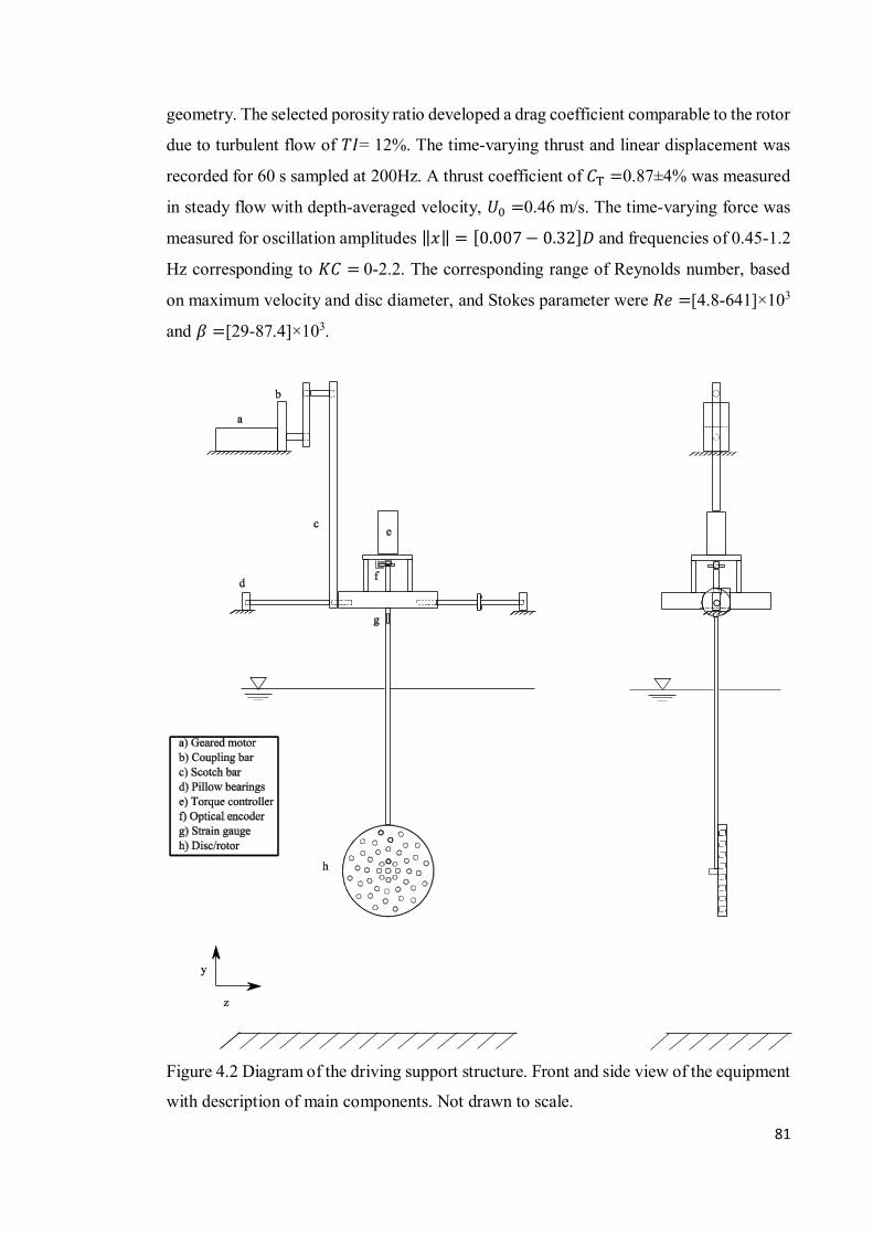
81
geometry. The selected porosity ratio developed a drag coefficient comparable to the rotor
due to turbulent flow of 𝑇𝐼= 12%. The time-varying thrust and linear displacement was
recorded for 60 s sampled at 200Hz. A thrust coefficient of 𝐶T =0.87±4% was measured
in steady flow with depth-averaged velocity, 𝑈0 =0.46 m/s. The time-varying force was
measured for oscillation amplitudes ‖𝑥‖ = [0.007− 0.32]𝐷 and frequencies of 0.45-1.2
Hz corresponding to 𝐾𝐶 = 0-2.2. The corresponding range of Reynolds number, based
on maximum velocity and disc diameter, and Stokes parameter were 𝑅𝑒 =[4.8-641]×103
and 𝛽 =[29-87.4]×103.
Figure 4.2 Diagram of the driving support structure. Front and side view of the equipment
with description of main components. Not drawn to scale.

82
4.5 Drag and Damping of Oscillating Porous Discs in Still Water
The hydrodynamic force on the disc is approximated as the measured force, 𝐹m, minus
the mechanical force associated with drag of the oscillating support, 𝐹mech,t. The
mechanical force is quantified prior to attachment of the disc in the same fluid condition
characterised by the 𝐾𝐶. Buoyancy forces on the disc are neglected due to the nearly
constant depth of immersion of the rotor. The equation of motion of the rotor based on
Eq. 2.50 and Eq. 2.52 is:
−23𝜔𝜌𝐷
3𝐶b�̇�−13 𝜌𝐷
3𝐶a�̈� = 𝐹m = 𝐹osc − 𝐹mech,t Eq. 4.5
The measured amplitude of the streamwise motion is determined as the amplitude
of a sine wave that is a best fit to the measurements using the least-squares method. The
angular velocity and acceleration of the disc in the streamwise motion are thus estimated
as the first and second time derivative of this fitted displacement. The hydrodynamic
coefficients (𝐶a, 𝐶b ) are obtained by Eq. 4.5 as the least-squares best fit equal to 𝐹m
(Figure 4.3).
Figure 4.3 Excitation force of disc due to sinusoidal axial oscillation in quiescent flow.
On the left axis, comparison of the measured (-) and predicted force (--) with the added
mass and damping force for one amplitude of oscillation. On the right axis, the velocity
of the disc due to forced motion in the streamwise direction (─).

83
The resultant added mass and damping coefficients from best fits with least-
squares residuals R2res >0.95 vary with 𝐾𝐶 for different Frequency numbers (Figure 4.4).
The damping coefficients for each 𝛽 case were found to increase almost linearly with 𝐾𝐶.
Linear trend lines obtained by a least-squares approach had slopes of 0.152 with only a
6% variation with Frequency number (Figure 4.4). In the test conditions studied, a small
phase difference was observed between the predicted velocity and the measured force due
to a low added-mass contribution (e.g. Figure 4.3). The added mass coefficients fluctuated
around a mean of 0.12 for the amplitude range, 𝐾𝐶<0.5, but exhibited greater scatter at
the higher amplitudes, perhaps due to a lower magnitude of the inertia relative to the
increasing damping force. A similar low added mass contribution is expected on a full-
scale rotor. It was also concluded from the review of heave studies of discs that increasing
the porosity ratio to 50% reduces greatly the damping (slope) compared with a solid disc
and the added mass becomes negligible.
Figure 4.4 Variation of added mass (left) and damping coefficients (right) against 𝐾𝐶 for
a disc of porosity ratio 0.52 at different 𝛽 numbers. x, 𝛽 =3.65×10⁶±5%; ◁,
𝛽 =4.37×10⁶±5%; +, 𝛽 =5.1×10⁶±5%; ●, 𝛽 =5.83×10⁶±5%; ◊, 𝛽 =6.56×10⁶±5%; ,
𝛽 =7.29×10⁶±5%; ▼, 𝛽 =8×10⁶±5%; ♦, 𝛽 =8.75×10⁶±5%. Best least-squares fit line of
the damping coefficients at each (-) and all Frequency numbers (─) using the linear force
of Eq. 4.5.

84
The oscillatory drag coefficients from the linear viscous damping force were
calculated from Eq. 4.1, Eq. 4.3, Eq. 4.4 and Eq. 2.52. A comparison was then made with
the force coefficients obtained from the measurements using the Morison equation (Eq.
2.39 and Eq. 2.44) with added mass normalised to a spheroid (Eq. 2.51). The oscillatory
drag coefficient and added mass coefficient were obtained with a least-squares fit giving
residuals within the range R2res>0.93.
Figure 4.5 Measurements compared to the average trend of the linear (--) and Morison
drag coefficient (─) in the quiescent flow with the 𝐾𝐶 number for different 𝛽 numbers.
Markers for 𝛽 describing the linear (thick edge) and drag coefficient (thin edge) are as
shown in Figure 4.4.
The linearised oscillatory drag coefficient across different 𝛽 was found to decay
exponentially with 𝐾𝐶 to the limiting magnitude of 2.22. For all the tests, the decay
formula given by a best least-squares fit was 𝐶D = 2.22 + 4.54𝑒−ξ𝐾𝐶 (Figure 4.5),
where ξ =9.61 represents the attenuation rate of the oscillatory drag with 𝐾𝐶, and its
magnitude, as stated by He et al. (2008), is proportional to the damping coefficient of the
plate. The attenuation rate varied with the 𝛽 employed, and this was within 13% of the
average trend. The highest discrepancy of the drag coefficient with the average trend
occurred at 𝐾𝐶 of 0.1-0.75 with the largest 𝛽 number employed. The Morison oscillatory

85
drag coefficient was similar and in good agreement with the linear viscous drag. It
decayed exponentially with 𝐾𝐶 to the limiting drag coefficient of 2.03. The mean added-
mass coefficient across the 𝐾𝐶 range of 0-2 was around 12% of that for a solid disc
(Figure 4.6). This behaviour was consistent with the results of Eq. 4.5.
Figure 4.6 Inertia coefficient in the quiescent flow using Eq. 2.39 and Eq. 2.44 with 𝐾𝐶
parameter and different 𝛽 numbers. Markers for 𝛽 number are as shown in Figure 4.4.
4.6 Drag and Damping of Oscillating Porous Discs and Rotors in Turbulent Flow
The time-varying force due to forced harmonic oscillation was also measured for the
porous disc and for a single rotor in turbulent channel flows of mean velocity 0.32, 0.39
and 0.46 m/s at the hub height. For some combinations of mean incident speed and
amplitude of streamwise oscillation, the minimum speed of the relative motion between
the water and rotor is lower than the operating speed for the rotor, which means angle of
attack is increased and stall would occur. Force on the rotor was therefore analysed for
conditions in which the rotor operated continuously, corresponding to a limited 𝐾𝐶 range
and velocity ratio, ‖�̇�‖𝑢0
< 0.5. However, force on the disc was measured for the same 𝐾𝐶

86
range as in still water. The stationary mean thrust of the disc in the turbulent channel
flows was 𝐹0 =5.5N±4% corresponding to a thrust coefficient 𝐶T =0.87±4%.
The presence of a mean flow changes the formation of the wake compared to
oscillation in quiescent fluid and so the drag due to oscillation in still water differs from
drag (or damping) due to oscillation in steady flow. Most authors (Chakrabarti, 1987;
Journée and Massie, 2001; Sumer and Fredsøe, 2006; Nakamura et al., 2013) address the
discrepancy by defining a Morison equation based on the relative axial velocity between
the water and the body as stated in Eq. 2.39.
However, several studies of rotors undergoing forced axial motion (Whelan et al.,
2009b; Milne et al., 2011) have stated that the excitation force is better represented as a
stationary disc in steady flow added to a force due to the relative axial motion between
the water and the rotor, 𝐹osc. The mechanisms involved in such observations and the flow
regime relationships acquired in the rotor between the mean flow and the axial motions
have not been fully understood.
The dynamic force was initially investigated using Eq. 2.39 and Eq. 2.46 with a
method similar to Eq. 4.5. This approach consisted of the axial force being equal to the
measured force, minus the mechanical drive and force on the tower
obtained, 𝐹mech,t~0.08𝐹0, without the disc, for 𝐾𝐶 in the range 0–1. The incident flow
had a constant velocity, 𝑢0. However, the simulations employing Eq. 2.39 and Eq. 2.46
were found to provide a poor approximation to the measured time-varying force with least
square residuals typically less than 0.4.
Following the alternative form of force (Eq. 2.49), the components of the relative
axial velocity between the disc and the water were then expanded, to treat the drag due to
the current and streamwise oscillation as separate forces. The volume of the rotor was
expressed with the water mass enclosed by a spheroid (Eq. 2.51).
In Eq. 2.49, drag force due to steady flow and drag force due to oscillator flow are
proportional to different drag coefficients. Furthermore, if the time-varying displacement
is provided by an equation such as �̇� = ‖�̇�‖ cos(𝜔𝑡) and the range of velocities is limited
to 𝑢0 > ‖�̇�‖. The first component of drag in Eq. 2.49 is:
𝐹D,1 =12𝜌𝐴𝐶D,1𝑢c
|𝑢c − �̇�| =12𝜌𝐴𝐶D,1𝑢c
2 −12𝜌𝐴𝐶D,1�̇�𝑢c
Eq. 4.6
From this arrangement, it is seen that the first expression on the right hand side
approaches the force acquired on a rotor that is rigidly supported in a mean flow with
turbulence present. Here, the drag coefficient is assumed to remain the same and is

87
defined analogous to the drag or thrust coefficient for the ambient flow with 𝑢0 =0.46
m/s, thus 𝐶D,1 = 𝐶D,c = 𝐶T =0.89 m/s. The second term in Eq. 4.6 becomes an extra force
with drag coefficient proportional to the velocity of the streamwise oscillation multiplied
with the turbulent current. For the speed ranges considered, the magnitude of this
force, 𝐹neglected,1 =12𝜌�̇�𝑢c𝐴𝐶D,1, is small when compared to the first term, and is thus
neglected. Following rearrangement and simplification, this first component of the drag
force, associated with the turbulent flow is (see Eq. 2.39 and Eq. 2.41):
𝐹D,1 ≈ 𝐹0 + 𝐹′ Eq. 4.7
where 𝐹0 =12𝜌𝐴𝐶D,c𝑢02 is a mean force and 𝐹′ = 1
2𝜌𝐴𝐶D,c(𝑢′
2 + 2𝑢0𝑢′) is the
force due to the turbulent fluctuations. For the second drag in Eq. 2.49, the drag
contribution of turbulent fluctuations is separated from the streamwise oscillation
component, by re-writing the turbulent current as the sum of a mean and a zero-average
fluctuation component (Eq. 2.40). This provides an arrangement, such that the second
drag is mainly attributed to a single force with drag coefficient, 𝐶D,2, which is proportional
to the multiplication of velocities between the relative flow (disc and water) and the rest
frame associated with the streamwise oscillations. The second component of the drag
force becomes:
𝐹D,2 = −
12𝜌𝐴𝐶D,2�̇�
|𝑢c − �̇�| = −12𝜌𝐴𝐶D,2�̇�
|𝑢0 − �̇�| −12𝜌�̇�𝑢
′𝐴𝐶D,2 Eq. 4.8
In Eq. 4.8, the force 𝐹neglected,2 =12𝜌�̇�𝑢′𝐴𝐶D,2 is assumed with a drag coefficient
similar to the first part. It remains small for the range of streamwise speeds considered
and is thus neglected.
The Morison equation for the disc and rotor subjected to streamwise oscillations
in a mean flow with turbulence, ignoring the small terms in Eq. 4.6 and Eq. 4.8, is
approximately due to the force of a rigid disc in the turbulent channel flow, which is then
added to a drag and inertia force due to the streamwise oscillations. The modified
expression is:
12𝜌𝐴𝐶T𝑢c
2 −12𝜌𝐴𝐶D,2�̇�
|𝑢0 − �̇�| −13𝜌𝐷
3𝐶a�̈� = 𝐹0 + 𝐹′ + 𝐹osc ≈ 𝐹m Eq. 4.9
This approach provided a best fit to the measured data with residuals greater than
0.85. To assess the accuracy of the oscillatory drag coefficient, the higher frequency
oscillatory forces, which are included in Eq. 4.9 as 𝐹′ only, were extracted from the

88
measured force using a third-order band-pass Butterworth filter. The oscillatory force was
defined for a frequency range with threshold values of ±20% of the frequency of forced
oscillation, 𝑓.
The hydrodynamic parameters for both the disc and single rotor in the turbulent
channel flows were then calculated from measurements using a best-fit force (Eq. 4.9)
with the least-squares residual R2res>0.92. The trend of the oscillatory drag coefficients
in the quiescent flow tests were also compared to the mean flow with turbulence present.
The variation due to the 𝛽 number was small and thus neglected.
Figure 4.7 The oscillatory drag coefficients obtained in the quiescent and mean flow
conditions with turbulence against 𝐾𝐶 number. □, disc in flow of 𝑢0 =0.35 m/s; ∆, disc
in flow of 𝑢0 = 0.39 m/s; ○, disc in flow of 𝑢0 =0.46 m/s. ■, rotor in flow of 𝑢0 =0.35
m/s; ▲, rotor in flow of 𝑢0 =0.39 m/s; ●, rotor in flow of 𝑢0 =0.46 m/s. Trend line of
oscillatory drag for quiescent flow using linear viscous (--) and Morison Equation (─).
The drag coefficient of the porous disc and single rotor in the turbulent channel
flows decayed exponentially with 𝐾𝐶 to a constant drag coefficient in an analogous
manner to the quiescent flow tests, thus 𝐶D,2 ≈ 𝐶D (see Figure 4.7). The trend line of the
drag coefficient using the linear viscous damping was above the measured results in the
highest mean incident speed but was in better agreement for the lower two speeds of
turbulent channel flow over the 𝐾𝐶 range 0.25–0.5.
89
The added mass remained close to zero across the studied flow conditions, 𝐶a ≈
-0.3 to 0.2. The negative values may have been due to the calculation method and the low
inertia relative to the damping force.
The Morison force (Eq. 4.9) was found suitable for the range of 𝐾𝐶<0.65 defined
with amplitudes of streamwise velocities, ‖�̇�‖, less than 0.5 times the mean flow, 𝑢0. For
this range, the magnitude of drag coefficient of the rotor in the turbulent flows was similar
to a porous disc that produces similar thrust coefficient in steady flows. The difference
between the drag coefficient for rotor and disc scattered at the range of 𝐾𝐶 < 0.65 was
approx. 12.5%. The discrepancy of results was due to the approximation of the non-linear
velocity and the neglected terms in the full Morison force (Eq. 2.39).
It can be inferred from Eq. 4.9 that at higher values of velocity ratios, ‖�̇�‖/𝑢0>0.5,
the influence of hydrodynamic forces over the mean current is greater and thus force
assumption would be less accurate at velocity ratios approaching the unity. Increasing
further the turbulence intensity would also cause variation of the drag coefficients due to
the neglected terms of turbulent fluctuations (𝐹neglected,2, see Eq. 4.8) that would become
relevant for small velocity ratios, ‖�̇�‖𝑢0≪ 0.5.
For the rotor, differences in thrust coefficients would be expected with change of
onset flow speed since a constant retarding torque is applied. As onset flow changes,
rotational speed, flow relative to the foil and resultant lift and drag of the foil also change.
For the rotor studied lift and drag may also vary with Reynolds number over the range of
onset velocities considered. However, the thrust coefficient of the rotor varies by less than
5% over a range of tip-speed-ratios 4-6. A full-scale rotor would be a different geometry
to develop the same variation of the scaled rotor thrust coefficient with tip-speed ratio.
Similarly a full-scale disc of different geometry may develop the same thrust coefficient
since the contribution of viscous effects may differ.
The drag of the scaled disc would be only different to a full-scale rotor if the
viscous effects of the porous disc in the same flow speeds cause a different drag and thrust
coefficient. Therefore, if the thrust coefficient of the disc is representative of the thrust
coefficient of the full-scale rotor, in the range of most onset flow speeds of interest. Then
the drag coefficient between the full-scale rotor and the equivalent disc would be the

90
same. The added mass for both disc and rotor has been measured small relative to the
drag force and its contribution can be neglected.
4.7 Extreme loads on Oscillating Rotors in Turbulent Channel Flow
An extreme prediction method is evaluated against rotor measurements due to forced
axial motion with high frequencies (0.7 Hz) against mean flow at highest speed with
turbulence. The methodology of Section 3.4 is applied to the thrust measurements to
obtain the magnitudes exceeded in 1 in a 100, 1 in a 1000, and 1 in a 10000 samples with
the Type 1 Pareto method. The extreme-value analysis was applied to samples of 420 s
duration. The range of tests represents large amplitudes of streamwise velocities up to
60% of the mean flow. This numerical approach consisted in using the findings of Eq.
4.9, for the determination of the peak forces such that the measured force is approximated
by:
𝐹m ≈ 𝐹0 + 𝐹′ + 𝐹osc Eq. 4.10
The extreme force on the rotor was calculated as the sum of peak forces resulting
from each component in Eq. 4.10. These values were then divided by the mean thrust (�̅�)
acquired in the forced streamwise motions with the incident flow. It is:
𝐹1n�̅�= [
𝐹0 + 𝐹′1n
�̅�] + [
𝐹osc,max�̅�
] Eq. 4.11
In Eq. 4.11, the first term denotes the force with probability of occurrence, 𝐹0 +
𝐹′1n, for a rotor operating in turbulent flow with no streamwise oscillation, whilst the
second term corresponds to the maximum force due to the relative axial motion between
the rotor and the water. The second force is modelled from Eq. 4.9 as:
𝐹osc = −12𝜌𝐴𝐶D�̇�
|𝑢0 − �̇�| Eq. 4.12
From Eq. 4.12 the peak rotor force occurs at the highest amplitude of combined
velocity from the streamwise motion and incident flow. It is:
𝐹osc,max =12𝜌𝐴𝐶D
‖�̇�‖(𝑢0 + ‖�̇�‖) Eq. 4.13

91
The variation of the time-average force in the operating flow was investigated for
a small range of velocities limited to ‖�̇�‖ ≪ 𝑢0. For the given velocity range, the
component of velocity in Eq. 4.12 is:
�̇�|𝑢0 − �̇�| = �̇�𝑢0 − �̇�2 = ‖�̇�‖ cos(𝜔𝑡)𝑢0 − ‖�̇�‖2 cos2(𝜔𝑡) Eq. 4.14
Therefore, averaging these components for a complete period:
1T ∫ cos(𝜔𝑡)dt = 0T/2
−T/2 and 1𝑇 ∫ cos2(𝜔𝑡)dt = 1
2T/2−T/2 Eq. 4.15
and substituting them into the components of the oscillatory force (Eq. 4.14). The
mean of the combined force from current and streamwise oscillation using the modified
Morison equation (Eq. 4.10) becomes:
�̅� = 𝐹0 +14𝜌𝐴𝐶D
‖�̇�‖2 Eq. 4.16
To verify the increase of mean thrust with velocity ratio, ‖�̇�‖/𝑢0, the thrust
coefficients measured in the three mean flows with turbulence present were compared
with predictions using Eq. 4.16. The thrust and drag coefficient employed for simulations
accounting the current and streamwise oscillations corresponded to 0.89 and 2
respectively. It was observed that the thrust for the disc remained similar to the rotor in
three current flows and for both rotor and disc, the mean thrust coefficient tended to
increase with velocity ratio (Figure 4.8). Predictions of increase of thrust were found
reasonable for the three mean flows with velocity ratios less than 0.5. A discrepancy was
observed in higher amplitude of motion and low incident flow speeds due to the lower
accuracy of the Morison force. The high velocity ratio resulted in a over prediction of the
mean thrust by Eq. 4.16.

92
Figure 4.8 Mean thrust coefficient against velocity ratio for disc and rotor. Predictions
using Eq. 4.16 (─). Markers of measurements as Figure 4.7.
After substituting the force terms from Eq. 4.13 and Eq. 4.16 into Eq. 4.11, the
extreme force is:
𝐹1n�̅�=𝐹0 + 𝐹′1
n+ 12 𝜌𝐴𝐶D‖�̇�‖(𝑢0 + ‖�̇�‖)
𝐹0 +14𝜌𝐴𝐶D‖�̇�‖
2
Eq. 4.17
The statistical influence of the turbulent fluctuations was obtained from rotor
measurements in turbulent flow without streamwise oscillations. The oscillatory force
was specified for the range of rotor surge oscillations with velocity ratios of ‖�̇�‖𝑢0=0–0.85
by using 𝐶D ≈2 for 0.25<𝐾𝐶<1. This range was selected to investigate the trend of peak
thrusts with increased streamwise velocity, extending beyond the range of conditions
studied experimentally for either rotor or disc. The predictions of force are in good
agreement (within 15%) with the measurements of the rotor operating in an incident flow
with turbulence present and without oscillation in the streamwise direction.

93
Figure 4.9 Predictions of the exceedance loads 1% (--), 0.1% (--) and 0.01 % (--) using
an oscillatory drag coefficient of 2 against measurements of rotor undergoing streamwise
oscillations in a mean flow with 𝑇𝐼 =12%. The 1-minute measurements of the 1% (●),
0.1% (+) and 0.01% (X) rotor forces are also shown against the 1% (-), 0.1% (-) and
0.01% (-) rotor loads obtained in a turbulent flow without streamwise oscillation.
From Eq. 4.17 and its derivative in respect to the streamwise velocity, the extreme
force increases from the values obtained due to turbulent channel flow only and tend to a
limit as the amplitude of the imposed streamwise oscillation approaches the incident flow
velocity (Figure 4.9). However, increasing the amplitude of oscillation further would
cause the minimum incident velocity to approach zero leading to stalling of the rotor. The
latter effect, resulting from the high angles of attack in which the blades operate, due to
the relatively low speed acquired between the rotor motion and the water. The rotor
loading was predicted well in the studied range using the Morison force of Eq. 4.11.

94
4.8 Summary
Measurements of added mass and drag coefficients were compared for a rotor and a
porous disc subject to forced oscillation in steady flow. The disc porosity was selected
such that the rotor and disc developed similar thrust coefficient in steady flow. The time-
varying force and displacement were obtained with a dynamic structure for both a rotor
and disc in turbulent flow of three different mean speeds and for the disc only undergoing
oscillation in a quiescent flow. The added mass and damping were made non-dimensional
by the mass of a spheroid. The variation of linear damping (Eq. 4.5) and Morison type
drag variation (Eq. 2.39) with Keulegan Carpenter number was studied and its effect with
small range of frequency number (Stokes parameter) was shown to be small.
For both a 3-bladed rotor and a porous disc that develops equivalent mean thrust,
the added mass due to oscillation in quiescent flow was approximately 12% of the mass
of a spheroid. Damping coefficient was a linear function of Keulegan Carpenter number
for 𝐾𝐶 < 2 and variation of this relationship with frequency number was less than 6%
(Figure 4.4). The oscillatory drag coefficient exhibited an exponential constant decay
form to a limiting value of 2 (Figure 4.5). This magnitude was found to be within the
range of oscillatory drag coefficients of 1.8-2.4 reported for a rotor undergoing
streamwise motion in steady flows which was described using an equivalent form of
Morison equation (Whelan et al., 2009b). The measured force in turbulent channel flows
was studied with a drag term using the Morison equation (Eq. 4.9). This approach
consisted in summing the force obtained on the rotor, when supported on a stiff tower in
a turbulent channel flow, with an oscillatory force using an oscillatory drag coefficient
based on the streamwise oscillation. Good agreement of drag coefficient was obtained in
the three turbulent channel flows between disc and rotor in the studied range of velocities
and amplitude of forced axial oscillations. The inertia of the rotor and disc was found to
be negligible in the turbulent channel flows. The mean thrust coefficient increased with
velocity ratio ‖�̇�‖/𝑢0, but remained close to the rotor thrust in turbulent channel flow
over the range ‖�̇�‖ < 𝑢0/2.
A reasonable approximation to the time-varying force on a rotor undergoing
forced oscillation in turbulent channel flow is obtained by summing the force of the rotor,
when supported in a stiff tower in turbulent channel flow, with a Morison type drag force
(Eq. 4.10) defined by the product of velocity amplitude and the maximum velocity,

95
‖�̇�‖(𝑢0 + ‖�̇�‖), and using a drag coefficient of approximately 2. This method was used
to assess the influence of the rotor oscillation amplitude on extreme forces due to imposed
oscillation within a turbulent channel flow. Rotor forces with 1 in 100, 1 in a 1000 and 1
in a 10000 probability of exceedance were shown to increase with amplitude of
streamwise velocity, with good agreement with measurements over the range ‖�̇�‖ <
𝑢0/2 and asymptoting to a limit at higher values of oscillation amplitude.
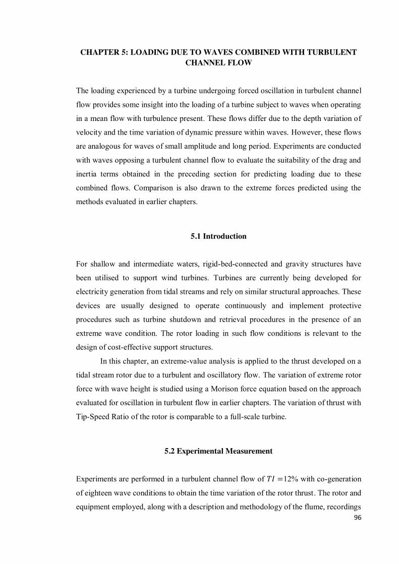
96
CHAPTER 5: LOADING DUE TO WAVES COMBINED WITH TURBULENT CHANNEL FLOW
The loading experienced by a turbine undergoing forced oscillation in turbulent channel
flow provides some insight into the loading of a turbine subject to waves when operating
in a mean flow with turbulence present. These flows differ due to the depth variation of
velocity and the time variation of dynamic pressure within waves. However, these flows
are analogous for waves of small amplitude and long period. Experiments are conducted
with waves opposing a turbulent channel flow to evaluate the suitability of the drag and
inertia terms obtained in the preceding section for predicting loading due to these
combined flows. Comparison is also drawn to the extreme forces predicted using the
methods evaluated in earlier chapters.
5.1 Introduction
For shallow and intermediate waters, rigid-bed-connected and gravity structures have
been utilised to support wind turbines. Turbines are currently being developed for
electricity generation from tidal streams and rely on similar structural approaches. These
devices are usually designed to operate continuously and implement protective
procedures such as turbine shutdown and retrieval procedures in the presence of an
extreme wave condition. The rotor loading in such flow conditions is relevant to the
design of cost-effective support structures.
In this chapter, an extreme-value analysis is applied to the thrust developed on a
tidal stream rotor due to a turbulent and oscillatory flow. The variation of extreme rotor
force with wave height is studied using a Morison force equation based on the approach
evaluated for oscillation in turbulent flow in earlier chapters. The variation of thrust with
Tip-Speed Ratio of the rotor is comparable to a full-scale turbine.
5.2 Experimental Measurement
Experiments are performed in a turbulent channel flow of 𝑇𝐼 =12% with co-generation
of eighteen wave conditions to obtain the time variation of the rotor thrust. The rotor and
equipment employed, along with a description and methodology of the flume, recordings

97
of the flow kinematics, axial force and rotor’s rotational speed is explained in Section 3.2.
The mean flow velocity, water depth and configuration of the rotor and support structure
in the wave conditions are all comparable to the turbulent channel-flow tests. Opposing
waves are specified with amplitudes [10-20] mm and frequencies [0.5-1] Hz by piston-
type wave paddles located 12.5 m from the inflow and 6.5 m from the rotor. The surface
elevation, 𝜂(𝑡), is recorded with a pair of wave probes located at the mid X-Y plane of
the channel flume, each 1 m apart from the rotor axis (Figure 5.1). For all tests, the motor
torque was specified such that the mean Tip-Speed Ratio, 𝑇𝑆𝑅, was 5.5 ±6%. For this
Tip-Speed Ratio range, the mean thrust coefficients obtained from recordings and
predictions using the BEM were 0.91 ±7% and 0.84-0.86. Time-varying parameters were
recorded at 200 Hz for a 60 s interval. Measurements were repeated 44 times for each
oscillatory flow.
Figure 5.1 Experimental arrangement for the sea states conditions. Waves are generated
at the right opposing the turbulent current flow. Rotor installed at mid depth with a pair
of wave probes recording the surface elevations.
5.3 Variation of Extreme Loads with Wave Height
The measured force is analysed to determine the force exceeded by 1%, 0.1% and 0.01%
of samples. Extreme value anlaysis methods of Chapter 2 are evaluated for all wave
conditions such that the extreme values obtained with different sample durations and
threshold magnitudes were within 3% of those obtained employing 44 minutes of

98
continuous thrust data. A threshold force of 1.25 times the mean force and 10 min sample
length was found to provide reasonable convergence of extremes. Higher values of
threshold values gave similar extreme results, but required larger samples. In Figure 5.2,
the sensitivity of the threshold against the sample duration is depicted for a wave
condition of a specified frequency 0.6 Hz and amplitude 10 mm. The return period of the
0.01% represented the force likely to occur in a full-scale turbine at long-run average
intervals of 48 hours during continuous rotor operation in the same flow. From recordings
of wave-gauge monitors, statistical heights and elevations (𝐻 ≈ 2√2𝜂rms) were utilised
to contrast the extreme loads acquired at the eighteen oscillatory flows. The highest
studied flow condition represented a wave height of approximately 10 m in a full-scale
turbine. Additionally, the measurements for the combined flow were compared to the
turbulent channel flow only (𝑇𝐼 =12%).
Figure 5.2 Difference in percentage of the 1% (left) and 0.1% (right) loads obtained with
different threshold forces and sample lengths based on the continuous 44 minutes of data
for waves specified with 0.6 Hz and amplitude of 10 mm opposing a mean flow with
turbulence present (𝑇𝐼 =12%).
The extreme thrust in the combined flows exhibited an approximately quadratic
increase with the amplitude of the wave. Waves specified with frequencies greater than
0.9 Hz did not propagate to the rotor due to their small velocity relative to the current and
so the extreme thrust experienced remained similar to the turbulent channel flow only.

99
The flow with wavelength 3.16ℎ (ℎ=water depth) and amplitude 0.12ℎ provided the
highest 1% thrust with a magnitude of 220% of the mean force in the turbulent channel
flow only. The spectrum of force in the combined flow for a small height regular wave
was studied and compared to the force imposed in a turbulent channel flow only. The
spectrum in the combined flow exhibited a comparable behaviour to linear sum of the
spectrum of force in turbulent channel flow with the narrow-band force spectrum that is
associated with the wave frequency (shown in Figure 5.3). Dominant frequencies in the
oscillatory flow corresponded to the specified wave frequency, 𝑓wave = 0.6 Hz, natural
frequency of the device, 𝑓n, the mean rotational speed 𝑓r =𝜔2𝜋
, and a harmonic of the
rotational speed, 3𝑓r, corresponding to the blade-passing frequency.
Figure 5.3 Force spectra for flow conditions without waves (-) and with waves of low
(--) and high amplitude of elevation (--). Peak frequencies correspond to the wave, 𝑓wave ,
mean rotational speed, 𝑓r, third rotational harmonics, 3𝑓r, and support natural
frequency, 𝑓n.
For conditions of wave heights above 0.26ℎ, the extracted power of the rotor was
low due to the high fluctuations of the incident flow velocity. For these wave conditions,
the thrust spectra exhibited a partial combination of forces due to overlapping of the
amplitude spectrum of the wave velocity with the ambient flow (Figure 5.3). This

100
produced a quadratic increase of the extreme thrust with the wave height, but to an initial
force lower than obtained in a turbulent flow without waves (see Figure 5.4). In practice,
turbines are likely to be shut down in the given flow conditions and so drag on the
stationary rotor and structure would be considered rather than thrust on the rotor.
However, this case was investigated to provide insight of extreme loads in a possible
operating condition.
Figure 5.4 The extreme load variation from the measured time-varying force compared
with the statistics of the surface elevations. The 1% (■), 0.1% (▲) and 0.01% (i) rotor
forces obtained in oscillatory flows due to a current opposing waves against the extremes
in flow of 𝑇𝐼 =12% (─) without waves.
The statistics of the wave heights and forces obtained in the eighteen oscillatory flows are
summarised in Appendix B.
5.4 Extreme Loads due to Turbulent Channel Flow with Waves: Drag Prediction
The Morison equation is an approach regularly used to analyse the forces occurring on
bluff bodies due to sinusoidal time-varying flows. The full Morison force is expressed as
𝐹m = 12𝜌𝐴𝐶D(𝑈a − �̇�)|𝑈a − �̇�| + 𝜌𝑉𝐶a(�̇�a − �̈�) + 𝜌𝑉�̇�a where 𝐴, 𝑈a, 𝑥, 𝑉, 𝐶a and
𝐶D denote the swept area, incident velocity, body motion, volume, the added mass and
drag coefficient of the body respectively (see Section 2.12). However, other alternative
101
forms of the Morison equation exist and have been addressed as more appropriate for the
wave loading on porous objects, which are representative of offshore jacket structures
and scaled tidal stream turbines (Whelan et al., 2009b; Taylor et al., 2013).
The loading on the rotor in turbulent channel flows combined with waves is
investigated on the basis of the extreme values of thrust, both measured and predicted,
based on the wave-induced hub-height velocity predicted assuming linear wave theory.
The force is given analagous to the Verley and Moe’s (1979) formula (see Eq. 2.48) by
summing the force due to the turbulent channel flow with an oscillatory force due to the
wave component of velocity only. The oscillatory thrust is expressed with a drag
coefficient of unknown magnitude, 𝐶D,wave , kinematics of the mean flow with turbulence
present, 𝑢c, and a thrust coefficient based on the turbulent channel flow, 𝐶T =0.89. The
inertia of the rotor is assumed to be small and is thus neglected. The force is:
𝐹 ≈ 𝐹turb + 𝐹p,wave ≈
12𝜌𝐴𝐶T𝑢c
2 +12𝜌𝐴𝐶D,wave𝑢wave
|𝑢wave| Eq. 5.1
For this method, the extreme force in the combined flow is due to the statistics of
the measured force in a turbulent flow, which are then added to the maximum force due
to the presence of the waves. The maximum thrust due to the wave kinematics only is
obtained as:
𝐹1n,wave
= 12𝜌𝐶D,wave𝜋𝑅2‖𝑢wave‖2 Eq. 5.2
where 𝑅 denotes the rotor radius and 𝑢wave is the amplitude of the wave velocity
at the hub height obtained from measurements (𝑢wave,m) or predictions (𝑢wave,p) of the
combined current and wave flow.
The wave velocity is predicted using linear wave theory and measurements of the
surface elevations in the combined flow. The oscillatory flow is modelled as opposing
waves propagating parallel to a mean flow of constant velocity (𝑈0) assumed constant
over the depth. Wave breaking, reflection and non-linearities are neglected. The
horizontal velocity for the oscillatory flow is expressed as (Phillips, 1977; Dean and
Dalrymple, 1991):
𝑢wave,p =(𝜔 − 𝑘𝑢0)𝐴wave cosh(𝑘(𝑧 + ℎ)) cos(𝑘𝑥 − 𝜔𝑡)
sinh(𝑘ℎ) Eq. 5.3

102
The variable 𝑧 represents the distance from the mean free surface (+ve upward),
ℎ represents the water depth and 𝐴wave the surface wave amplitude. The angular
frequency, 𝜔, is estimated with the Doppler effect:
𝜔 = 𝑈0𝑘 + √𝑔𝑘 tanh 𝑘ℎ Eq. 5.4
where 𝑔 is the gravity constant and k is the wave number obtained relative to a
reference frame moving with the mean flow speed. The amplitude of the wave height is
estimated from the peak amplitude of the spectra measurements of the surface elevations.
Wave conditions in which breaking waves occurred were not considered. The assumed
wave height range is ‖𝜂‖ℎ
<0.05. This linear prediction was in good agreement with
measured kinematics at hub height, to within 7% for the small amplitude waves
considered in the extreme force analysis (Figure 5.5).
Figure 5.5 Comparison of the measured and predicted amplitude of wave velocity at the
hub height (■) using linear wave theory and measurements of the surface elevations.
Subsequently, the drag coefficient was determined using Eq. 5.2 with the predicted
amplitude of the wave-hub velocity, as a best-fit approach of the measurements of
extreme rotor force in the combined flow (Figure 5.4). For this method, a drag
coefficient, 𝐶D,wave = 11 provided the 1%, 0.1% and 0.01% and steady flow thrust
coefficient of 0.89 provided forces to within 8%. The uncertainty of the drag coefficient

103
due to discrepancy of predicted hub velocities against kinematic measurements (7%) was
also considered. For this purpose, Figure 5.6 depicts the uncertainty of the peak thrusts
with velocity magnitude (smaller markers) and contrasts this with the extreme force
simulations accounting for velocity variation (using Eq. 5.2). This approach provided
different fitted drag coefficients (shown in bands) and the mean of these lines remained
with a value of 11.
Figure 5.6 The measured exceedance forces in waves with probabilities of 1% (■), 0.1%
(▲) and 0.01% (i) and same forces (□, ∆, ◊) due to uncertainty of the wave velocities
±7%. Simulations are shown using wave kinematics with a drag coefficient of 11 (--) and
a range of drags accounting for velocity variation of 7% (█). Extreme loading in turbulent
channel flow of 𝑇𝐼 = 12% (─) is also compared.
5.5 Time-varying Kinematics and Drag due to Waves and Turbulence
The loading on a rotor is known to be dependent on the pressure drop across the rotor and
this is dependent on the flow characteristics occurring along the rotor’s blades and
downstream. Unsteadiness in an onset flow for a tidal stream turbine is due to several
processes and these result in unsteady loads. Waves alone impose dynamic wave
pressures and accelerations both varying in time and space whilst the current alone may

104
contain depth variation of flow and high-frequency fluctuations due to turbulence
(McCann et al., 2006). Although several studies have assumed minimal interactions on
the average thrust imposed on a rotor in uniform flow and combined uniform flow with
waves, little has been done on the interactions of the extreme rotor loads due to the waves.
In this section, the forcing in waves combined with turbulent channel flows is investigated
in an analogous manner to the loading on a rotor undergoing forced streamwise
oscillations in turbulent channel flows (Chapter 4). This approach suggests that the rotor’s
response in waves combined with turbulent flows is approximately given as the sum of a
thrust in ambient flow and a drag due to the relative wave velocity predicted at the hub
height. However, for flows combined with waves, the wave velocity over the channel
depth decays in proportion to the height and frequency of the surface wave. This effect
of varying velocity over the rotor is not considered. Therefore, for the wave conditions
with small wave heights and wave numbers, such as 𝑘ℎ →< 𝜋/10 (see Eq. 5.3), the
thrust assumption may be found acceptable.
Time varying force due to waves with turbulent flow is modelled using the
Morison force described in Section 4.6, by replacing the axial motion of the rotor with
the wave-induced component. To evaluate its suitability against rotor measurements in
waves and thus compare the oscillatory drag with the findings of using Eq. 5.2. The thrust
due to wave kinematics, 𝐹osc, is extracted from the measurements using the band-pass
filter techniques of Section 4.6. The added mass of the rotor and support is ignored.
The wave kinematics are predicted with the linear wave theory as explained in
Section 5.4 and the drag force due to relative wave velocity becomes:
12𝜌𝐴𝐶D,wave𝑢wave,p|𝑢0 − 𝑢wave,p| = 𝐹osc,p Eq. 5.5
The magnitude of the drag coefficient for small wave conditions is obtained as the
least-squares fitting of Eq. 5.5 with the measured wave force, 𝐹osc. The comparison
between measurements and simulations using this approach for a wave condition is shown
in Figure 5.7.

105
Figure 5.7 Time-varying force due to waves against predictions employing linear wave
kinematics at the hub height. --, predictions;─, measurements.
Drag coefficients with the least square fit residuals above 0.9 were selected and
plotted against the operating 𝐾𝐶, based on the frequency and amplitude of the wave
velocity at the hub height (Figure 5.8). The wave loading in turbulent channel flows
produced time-varying forces and oscillatory drag coefficients of 2 with standard
deviation of 0.0805. These values were comparable to a rotor subjected to streamwise
oscillations in a flow of the same 𝑇𝐼 =12% with drag coefficients tending to a magnitude
of 2 with increasing 𝐾𝐶 number (shown in Section 4.5). The flows were concluded to be
analogous.

106
Figure 5.8 The oscillatory drag (X) of a rotor on a fixed support structure in turbulent
channel flow with opposing waves. 𝐾𝐶 based on hub-height velocity predicted by linear
theory from measured wave height.
5.6 Prediction of Extreme Loads based on Forced Streamwise Oscillations of the
Rotor in a Turbulent Channel Flow
The prediction method of extreme force described in Section 4.7 for a rotor subjected to
streamwise oscillation is evaluated against the loading for a rotor in waves opposing a
turbulent channel flow without forced streamwise oscillations. This approach shows that
the force distribution due to streamwise oscillation in turbulent channel flow is
approximately due to the peak thrust based in mean flow with turbulence present, which
is then added to the maximum value of the wave-induced drag, 𝐹osc, defined by relative
velocity and using a mean oscillatory drag, 𝐶D =2, for the amplitudes of surge oscillation
given in the 𝐾𝐶 range 0 to 1. The extreme force, quantified in proportion of the mean
thrust of the combined flow, becomes:
𝐹1n= [
𝐹0+ 𝐹′1n
𝐹] + [𝐹osc,max
𝐹]
Eq. 5.6
Here 𝐹′1n is the peak force measured due to turbulent channel flow only and
𝐹osc,max is by Eq. 5.5. The 1%, 0.1% and 0.01% predicted forces with this method were
compared against measurements of extreme thrust in turbulent channel flow combined
0 0.1 0.2 0.3 0.4 0.5 0.6 0.7 0.8 0.9 1 1.1 1.2 1.31
1.2
1.4
1.6
1.8
2
2.2
2.4
2.6
2.8
3
KC
CD
,wav
e

107
with wave and turbulent channel flow only (Figure 5.9). The curves of the peak loading
departed from the statistical forces in the turbulent channel flow and headed towards a
horizontal limit as the wave velocity amplitude approached the mean incident speed (as
shown in Figure 4.9). The rotor loading was predicted well with the Morison approach
using an oscillatory drag coefficient of 2 for the time-varying force and a thrust coefficient
of 0.89 for the mean force. The discrepancy of results was only 5.6% employing velocity
at the hub height with a discrepancy of 7%.
Figure 5.9 Predictions for the 1% (--), 0.1% (--) and 0.01% (--) wave forces using an
oscillatory drag coefficient of 2 against measurements of a rotor supported on a stiff tower
in a mean flow with 𝑇𝐼 =12% and opposing waves. Measurements of the 1% (□), 0.1%
(∆) and 0.01% (+) rotor wave forces against the exceedance loads in turbulent channel
flow without waves (─).

108
5.7 Summary .
A set of experiments was conducted to investigate the loading in representative tidal
characteristics of turbulent channel flow with opposing regular waves. The mean thrust
coefficient in the oscillatory flow conditions was found to be comparable to predictions
in uniform flow using the BEM method. A Type 1 distribution method with a Pareto tail
fitting technique was employed to determine the 1%, 0.1% and 0.01% rotor forces divided
by their mean. These maximum forces were obtained with a peak-over-threshold
technique. A threshold of 1.25 times the mean force was selected for all the turbulent
wave conditions. For this approach, a 10-minute sample was required to ensure
convergence of extremes within 3% of the values obtained from continuous 44 minutes
data. The maximum 1% force was encountered with the wave frequency condition of 0.7
Hz and had a magnitude of approximately 220% of the mean force. The extreme loading
in the combined flow showed an approximately quadratic growth with the amplitude of
the wave velocity and as wave velocity decreased, the force approached to the condition
in a mean flow with turbulence present only.
A drag term (Morison Eq.) was employed to investigate the rotor loading in
turbulent channel flows with opposing waves. This method was based on the rotor tests
undergoing streamwise oscillation in turbulent flow (Eq. 4.9), in which velocity of rotor
was imposed by forced oscillation and the resultant force was predicted by summing the
peak thrust due to turbulent channel flow with a maximum force defined by relative
velocity due to the wave. The simulations of extreme loads employed a thrust coefficient
of 0.89 for the turbulent channel flow and a drag coefficient of magnitude 2 for the wave
condition. The extreme forces departed from the statistical turbulent forces and asymptote
to a limit with increasing amplitudes of wave velocity. Extreme forces predicted using
Eq. 5.6 were within 6% of measurements, within the uncertainty associated with the
prediction of hub-height velocity from linear kinematics.

109
CHAPTER 6: SUPPORT-STRUCTURE DYNAMICS
In this chapter, the influence of support platform dynamic response on the loading of
horizontal-axis turbines is investigated by time-domain solution of a one and two-degree-
of-freedom coupled equation of motion. The particular interest is the influence of the
support-structure dynamics on the response and extreme loads experienced by a tidal
stream turbine when subjected to a combined turbulent channel flow with opposing
waves. The intention is to identify support structure properties that reduce the variance
and peak value of rotor thrust, to inform design optimisation of floating platforms.
Dynamic response is caused by wave forcing on the immersed part of the
supporting platform and loading on the rotor. Forcing on the rotor is modelled following
the approaches of Chapter 4 and 5. The onset velocity encountered by the turbine is time-
varying due to a combination of mean flow, turbulence, waves and the support-structure
motion. Response is modelled for two different systems: surge only and coupled surge
and pitch. The single mode model provides identification of the properties of a supporting
platform – specifically wave induced excitation force, radiation damping, stiffness and
added mass – that would reduce peak force on the turbine in comparison to a rigid
structure, such as a bed-connected support. The dynamic response for the coupled surge
and pitch motion is applied to a typical semi-submersible structure. Hydrodynamic
parameters for the support are obtained by linear diffraction theory. To assess benefits of
the dynamic response, a comparison is made of the mean variance of thrust between the
semi-submersible platform and a bed-mounted support in a wave condition representative
of tidal stream sites.
6.1 Introduction
Many of the offshore wind and prototype tidal stream turbines that have been developed
employ either gravity support systems or stiff bed-connected structures and have been
located in shallow and intermediate water depths, typically less than 30 m. Exploitation
of the deeper sites is the aim of many wind-farm projects (DEA/CADDET, 2000), but
employing the conventional turbine supports is both impractical and expensive. Several
floating moored systems have been proposed to support one or more turbines but these
have not yet been widely deployed at offshore sites. For these platforms, the rotor may

110
oscillate relative to a fixed reference due to mooring line deformation, excitation of the
support structure by surface waves and excitation of the rotor by unsteady loads during
operation. The reliability and design life of a turbine is dependent on the magnitude and
frequency of occurrence of the loading experienced during the design life (McCann, 2007;
Val et al., 2014). To inform design, it is important to predict dynamic response of the
floating system with sufficient accuracy to ensure reliability, stability and safe keeping of
the device. Several numerical tools accounting for rotor and support response are being
evaluated to gain understanding of the complex, dynamic behaviour (Francis and
Hamilton, 2007; Way et al., 2013; Van der Plas, 2014). The extent to which dynamic
response may mitigate the peak loads experienced by a turbine during operation has not
been documented and this is the aim of the present chapter.
6.2 Support Structures for Horizontal-Axis Wind and Tidal Stream Turbines at
Shallow and Intermediate Water Depths
Wind turbines are a mature technology that has been widely deployed onshore and,
particularly in Europe, at offshore locations. Compared to onshore, offshore sites offer
greater resource (Troen and Petersen, 1989), more predictable winds, little visual impact
and typically, the operating flows have lower levels of turbulence. The support structure
is required to resist the thrust due to wind variation, the compression forces by turbine
weight, and induced wave-current loads. Many of the offshore wind farms are located on
sandbanks and so driven monopiles are commonly used. Alternatives include braced
piles, tripods, suction caissons and heavy gravity foundations (Figure 6.1).

111
Figure 6.1 Different concepts of support structures for wind turbines deployed at shallow
water depths. Source from Musial and Ram (2010).
Design and deployment of tidal stream turbines is largely based on the experience
gained from development of wind turbines at offshore sites. The majority of the prototype
systems currently in development are horizontal-axis turbines rigidly fixed to the seabed
in a similar manner to wind turbines (Figure 6.2). Due to the speed of tidal streams, the
bed material at tidal stream sites is often scoured rock. Therefore, braced monopiles or
tripods are preferred. The magnitudes of rotor loading for wind and tidal turbines differ
and so different support design criteria apply. Winter (2011) shows that the mean thrust
on a tidal stream turbine rated at 1 MW is 6.4 times higher than that imposed on a wind
turbine of the same rated power. Tidal turbine blades may thus be designed for higher
ultimate and fatigue criteria than wind turbines.
It is not trivial to identify a single structure type that is most suitable for tidal
devices, since total costs are determined by several aspects, such as the structure material
and fabrication, as well as the costs of installation, maintenance and retrieval. Each
support structure requires sufficient stability to counteract the wave-induced loading and
the turbine cyclic thrusts. Orme and Masters (2006) compare six alternative support
structure types for tidal stream turbines in terms of the system cost and benefit. For each
system, the name and description is summarised as:
x Telescopic system - a tidal turbine mounted on a set of telescopic towers, which
can be expanded or contracted to adjust the height.

112
x Guyed tower - a tidal turbine with a self-buoyant nacelle bounded by four chains
attached to the sea floor.
x Top mounted - a tidal turbine supported on a fixed tower with the hub height at
mid-depth (e.g. Figure 6.2b, Figure 6.2c).
x Shrouded concept - a tidal turbine inside a venturi-type duct.
x Sheath - a turbine supported on a tower where it can slide all the way upwards and
downwards (e.g. Figure 6.2a).
x Anchored system - a tidal turbine chain anchored and kept in position with the
nacelle’s buoyancy.
Figure 6.2 Concepts and illustrations of fixed supported configurations a) Marine Current
Turbine (MCT Ltd) b) Alstom Tidal stream Turbine (Walker et al., 2013) c) a gravity
based concept (Atlantis Resources Ltd).
A key factor affecting the total cost of bed-connected supporting structures is the
cost of deployment since this is typically dependent on use of specialist vessels. Most
bed-connected structures appear to be prohibitively expensive when deployed in deeper
waters. In addition, the deployment of monopiles above 25 metres depth has not been
proven to withstand the large moments and shear stresses that will be generated by the
thrust imposed on a turbine (de Vries and Krolis, 2007). For surface-piercing structures,
wave-breaking effects encountered at intermediate depths magnify the horizontal force of
the reaction support almost up to 3 times, when compared to the non-breaking wave
condition (Stansby et al., 2013). These constraints to bed-connected structures have
motivated the development of alternative floating concepts for tidal turbines.
(a) (b) (c)

113
6.3 Floating Support Structures for Horizontal-Axis Turbines
Several floating and moored platforms are now in development as an alternative approach
to rigid-bed-connected structures. Examples of moored systems are given in Figure 6.3
and Figure 6.4. These structures allow small rotation of the platform resulting in
approximately linear displacement of the rotor with the requirement to provide stability
in all operating conditions. However, the extent of rotor motion and of dynamic loading
may affect the reliability and integrity of the gearbox, blades, bearings and nacelle.
Modern turbine designs typically permit a higher amplitude of the rotor pitch during
operation in comparison to a rigidly supported turbine. For example, dynamic operation
is acceptable for pitch of the rotor of up to 9 degrees from the vertical (Berthelsen and
Fylling, 2011).
Figure 6.3 Demonstration systems for deep-water regions. Different floating structures
denoting a 1) semi-submersible type 2) spar buoy design 3) Tension leg platform 4) TLP
gravity 5) spar system. Source from Musial and Ram (2010).
The different types of floating system can be classified by the operational means
for achieving stability: the ballast, mooring and buoyancy class. Several technical reports
have described their status, total costs, possible environmental effects, and the

114
engineering challenges usually encountered (Henderson et al., 2010; Butterfield et al.,
2007; Laura and Vicente, 2014). These can be summarised as:
x Ballast class - uses the weight of ballast placed below the water, to counteract the
moment due to turbine and tower force and thus minimise the oscillation
response. The minimum depth required is normally above 150 m. A typical
support is the spar buoy (Figure 6.4a). The disadvantages can be the high capital
cost and the reaction to wave and external loads.
x Tension leg type - mooring lines attached to the seabed provide sufficient tension
to stabilise the system. A common example is a tension leg platform, TLP, which
restrains vertical motions but allows small horizontal displacements and
rotations. The depth of deployment is above 50 metres and is considered as a
practical approach in terms of present offshore experience. However, anchor
failure leading to slack mooring lines compromise the stability of the whole
system.
x Buoyancy - the structural arrangement and water plane area are selected to
counteract the applied overturning moment and dynamic loads. The semi-
submersible structure with wind turbine above or tidal turbine below (Figure
6.4b) is an example of this concept. Typically these systems are slack-moored.
The main advantage of this method is the low draft which simplifies deployment.
Additionally, some electrical components could be placed in compartments above
the free surface to minimise corrosion and to facilitate maintenance of the system.
The disadvantages of a buoyancy-mooring device are the high reaction to waves
and external loads, the uncertainty in the dynamic response and the design of
appropriate engineering tools.
Turbine system designs are still evolving and, as a result, progress in this field has
been increasing. Perhaps the earliest trial of a floating platform, is the Hywind system
(Sun et al., 2012), which has been tested offshore for nearly two years (Figure 6.4a). This
2.3 MW wind turbine was constructed by the Norwegian Statoil Hydro Company and had
a spar buoy support 120 m long. It has gained considerable offshore experience and
multiple devices are currently undergoing trials as part of a small farm.

115
Figure 6.4 Floating offshore turbines configurations for wind turbines at deep waters a)
Deployment of Hywind spar buoy turbine (Sun et al., 2012). b) Novel concept of a
floating offshore turbine for deep waters (Weinstein et al., 2012).
Another concept is the semi-submersible WindFloat designed by Principle Power
Inc. (Weinstein et al., 2012; Roddier and Cermelli, 2014). The system supports a 2 MW
turbine and employs conventional anchoring and mooring lines. The platform consists of
three cylindrical floats connected by a rigid triangular framework. The damping and
buoyancy properties of the cylinders reduce the dynamic motion and maintain the turbine
in a vertical position. The scope of deployment is for intermediate and deep waters.
Floating structures similar to those proposed for wind turbines have been
proposed for deployment of tidal turbines. An advantage of such support structures is that
the turbine will be self-aligning with the incident flow. Furthermore, due to the typical
vertical profiles of velocity at tidal sites, the velocities in the upper region of the water
depth are typically greater than near the bed surface, thus increasing the kinetic energy
flux available at hub height. Perhaps the main advantage is that the cost of deployment,
retrieval and removal may be substantially lower than for fixed seabed foundations.
Several concepts employ the buoyancy of a component such as the nacelle to keep
the structure afloat, whilst depth of immersion is controlled through the length of taut
bed-connected mooring. The prototype devices TidEL (Ben Elghali et al., 2007) and
CoRMaT (Clarke et al., 2009) are based on this approach. TidEL comprises two contra-
rotating turbines located side-by-side downstream of a buoyant crossbar which is taut
moored to the seabed. The unit is intended for operational water depths greater than 30
metres and has a nominal rated power of 1MW. By contrast, CoRMat comprises a
buoyant single body with two contra-rotating turbines arranged in-line with very small
(a) (b)

116
streamwise spacing, of the order of 0.1 diameters. Both rotors operate a single direct-
drive generator and two rotors are employed to maximise generator speed for a given
flow-speed and to minimise net torque. The support structure is minimal, comprising only
a buoyant nacelle and a taut mooring, however stability during operation remains a design
issue (Clarke et al., 2010).
Other semi-submersible floating platform concepts have been proposed, such as
ScotRenewables (Keysan et al., 2010) and BlueTEC (Van der Plas, 2014). These
structures are located at the free surface and are rigid, typically with slack moorings,
which may be beneficial for protecting the device and for providing rotor stability with
the damping properties of the support. The ScotRenewables prototype comprises an
approximately cylindrical tube aligned with the flow direction and with two vertical arms
at the stern supporting turbines. The geometry of the structure creates minimal drag with
the waves that are propagated in-line with the rotor. It has more reaction to the surface
waves but also provides a large moment to counteract the turbine’s response. The main
advantage is that the system allows protection from peak loads and undesirable operating
conditions by raising an arm that supports each turbine (Scotrenewable Tidal Power Ltd.).
The BlueTEC design is analogous to the ScotRenewables and is also intended as a generic
slack moored system to provide stability for supporting either two horizontal or vertical-
axis turbines.
In order to support the development of tidal stream turbines on the floating
platforms, several design and operating issues need to be established. These include the
prediction of the variance and mean rotor loading in uniform flow, turbulent flow, and
waves combined with mean flow as well as dynamic loading due to rotor oscillatory
motion. Likewise, it is necessary to account for the effects of structure response in waves
combined with a mean flow that has turbulence present and the coupling of this motion
with the rotor response. In general, it is desired for a support structure to have a large
water plane area, a low centre of gravity, and natural period distinct from the wave period
to minimise motion due to waves.
Since a tidal stream turbine is located underwater, there are also other design
issues to consider which do not affect wind turbines. These include the selection of the
blade materials (Grogan et al., 2013), prevention of cavitation (Bahaj, Molland, et al.,
2007), bio fouling (Walker et al., 2014) and corrosion.

117
6.4 Floating Platform Dynamic Models
At present, a few numerical models account for the mooring load and the coupling of
support structure and rotor. For these dynamic models, the force on the rotor has been
modelled using BEM (Way et al., 2013) and CFD methods (Francis and Hamilton, 2007),
in order to predict the response of scaled semi-submersible systems, such as the Bluetec
(Van Riet Bergen et al., 2013; Van der Plas, 2014), ScotRenewables (Francis and
Hamilton, 2007) and other mooring concepts (Hayman et al., 2013), in flow conditions
that are representative of tidal stream sites. These approaches have been used to model
loading of two rotors attached to a semi-submersible structure located at the free surface,
under the assumption that the thrust from each turbine is self-aligning with the mean flow
and limits to a large extent the yaw moment applied to the support structure. If the heave
response and velocity variation of the wave-current flow over the rotor is small, only the
surge and pitch motion of the dynamic support contribute significantly to the rotor’s
variation of incident flow and hence affect the developed rotor thrust (Van der Plas,
2014). For a surface-piercing support platform, the tower supporting each rotor will also
add thrust moments and oscillations to the system which must be counteracted by the
mooring lines and dynamic response of the support.
The force ratio obtained between the rotor and the semi-submersible support due
to uniform flows of different speeds, in which the range of the flow speeds is within the
time-varying velocity of the wave-current flows, has been reported to be as much as 4 to
15 (Way et al., 2013). Therefore, the prediction of rotor force due to combined waves,
mean flow and streamwise oscillations plays a crucial role in the design of tidal floating
supports.
An approach to predict the dynamic response of a floating support, as followed
here, consists of decoupling the rotor forces from the structure dynamics and then
incorporating the rotor loading, support loading and external constraints into a coupled
model (see Figure 6.5) of system response. The characteristic length of the supporting
platform is typically greater than one-fifth of a wavelength, 𝐷 > 0.2𝐿w. As such wave
induced forcing is in the diffraction regime and viscous effects are typically neglected.
The response of the support structure develops a radiation damping force defined by
forcing of the body in still water 𝑋h,i,j = −𝑎i,j�̈�j − 𝑏i,j�̇�j, where 𝑎i,j and 𝑏i,j denote the
added mass and damping of the support platform oscillating with complex velocity

118
amplitude �̇�j. This is linearly superposed with the wave-induced force on the body when
held stationary in regular waves 𝑋i. Here, the subscript i=1…6 denotes the force or
moment corresponding to surge, sway, heave, roll, pitch and sway and j=1…6 the
components of the coupled motion in the same notation. The excitation force from n, the
number of rotors is obtained using a Morison equation based on relative velocity at the
rotor, following the approach of Chapter 4.
Figure 6.5 Scheme of the forces modelled from the floating system for six-degree freedom
of motion.
The force on the rotor is then dependent on the inertia and drag force from the
drive train, 𝐹I,11, 𝐹D,11, which are dependent on the added mass and drag coefficient,
𝐶a, 𝐶D, the mean flow velocity (𝑢0), the wave induced velocity, (𝑢wave,p) and the velocity
of the rotor in surge mode (�̇�rotor,1) due to surge (�̇�1) and pitch (�̇�5) of the supporting
platform. The force due to turbulent fluctuations is not simulated. Instead, the force
associated with the turbulent predictions (𝐹′, 𝐹′1n) is superposed with the simulated force
due to steady flow, waves and response. This approach was shown to provide reasonable
prediction of peak force due to oscillation in turbulent flow in Chpater 4 and due to
turbulent flow with waves in Chapter 5.
-Stiffness due to mooring lines-Restoring Forces
Hydrodynamics:-Wave Radiation -Added mass
Support Structure ResponseExternal Forcing
Response of Rotor supportedon a Stiff Tower
Force on Rotor Undergoing Streamwise Oscillations:-Damping or Oscillatory Drag -Added mass
L
X i,j
D

119
The force on a rotor, 𝐹I,11 + 𝐹D,11, is approximated with drag and added mass
coefficients of 𝐶D = 2 and 𝐶a =0.12 over the 𝐾𝐶 range 0 to 2 (see Chapter 4). In Chapter
4, the added mass was normalised to the water mass of a spheroid enclosing the rotor ,
𝑀a =13𝜌𝐷3. To facilitate solution of an equation of motion, it is convenient for all the
masses to be consistent. Herein the added mass coefficient is thus expressed in terms of
the water mass enclosed by a thin disc, 𝜌𝑉 = 14𝜋𝐷2𝑡h where 𝑡h = 0.022𝐷 is the thickness
of the disc, as per the Froude-Krylov force. The added mass coefficient is 𝐶′a =
0.12𝑀a𝜌𝑉= 2.28. The inertia and drag force per rotor is obtained from Eq. 2.39 and Eq.
2.47.
The general equation of motion for the rotor is obtained by coupling a six-degree-
of-freedom equation of motion for the floating support (Faltinsen, 1993; Journée and
Massie, 2001) with rotor forcing, inertia and damping:
∑(𝑚i,j + 𝑎i,j)�̈�j
6
j=1
+n𝑚rotor,i,j�̈�rotor,j + 𝑏i,j�̇�j + 𝑐i,j𝑥j = 𝑋i + 𝑋e,i
+ n𝑋D,i,j(�̇�rotor,j, 𝑢0, 𝑢wave,p) + n𝑋I,i,j(�̈�rotor,j, �̇�0, �̇�wave,p)
Eq. 6.1
where 𝑋D,i,j and 𝑋I,i,j correspond to the force or moment due to the drag and inertia
of the rotor in the six coupled modes. Restoring force and moment of the support
structure, 𝑐i,j, is due to the buoyancy forces in each mode. External forcing, 𝑋e,i, is applied
to the system to represent, wave drift and other non-linear effects such as mooring line
constraint. The response from the mooring lines is approximated as a spring with a
constant stiffness, 𝑘i,j𝑥j.
The particular focus of this study is the effect of waves and induced motion of the
support on the peak value of rotor thrust. This may be either, increased or decreased due
to the combination of turbulent flow and oscillatory flow due to both wave-induced
kinematics (Chapter 5) and due to motion of the rotor rigidly connected to the supporting
platform (Chapter 4). It is desirable to identify the support platform properties that would
result in a reduction of rotor response in slowly-varying oscillating motions that are
representative conditions for tidal flows.
The investigation is limited to two modes of support platform response – pitch
and surge. Motion in other modes would affect rotor orientation but would have limited
influence on velocity normal to the rotor plane. The length of the tower, 𝐿, is considered

120
large compared with the rotor displacement and so the pitch oscillation imposed on the
support is approximated as surge of the rotor thus 𝑥rotor,1 = 𝑥1 and 𝑥rotor,5 = 𝑥5𝐿 .
The equation of motion for surge is (i=1):
∑(𝑚11 + 𝑎1j)�̈�jj=1,5
+n𝑚rotor,11�̈�rotor,j + 𝑏1j�̇�j + 𝑐1j𝑥j + 𝑘1j𝑥j = 𝑋1 + 𝑋e,1
+ n𝐹D,1j(�̇�rotor,j, 𝑢0, 𝑢wave,p) + n𝐹I,1j(�̈�rotor,j, �̇�0, �̇�wave,p)
Eq. 6.2
and for pitch (i=5)
∑(𝑚55 + 𝑎5j)�̈�jj=1,5
+n𝐿𝑚rotor,11�̈�rotor,j + 𝑏5j�̇�j + 𝑐5j𝑥j + 𝑘5j𝑥j = 𝑋5
+ 𝑋e,5 + n𝐿𝐹D,1j(�̇�rotor,j, 𝑢0, 𝑢wave,p)
+ n𝐿𝐹I,1j(�̈�rotor,j, �̇�0, �̇�wave,p)
Eq. 6.3
A typical platform is then approximated using a horizontal circular cylinder of
length 5𝐷 and width 𝐷 with hemispherical ends of radius of the half width (0.5𝐷). A
diameter 𝐷 = 0.27 m is considered consistent with the lab-scale studies of previous
chapters. The length of the tower is 3 times the rotor diameter. The system modelled here
is approx. 1:70th scale based on the rotor’s diameter. The support is intended for
operational water depths of 60-80 metres such as found in the deep Pentland Firth. The
configuration of the semi-submersible structure supporting two contra-rotating rotors is
as shown in Figure 6.6. These dimensions are indicative of the systems studied by Van
der Plas (2014) and Francis and Hamilton (2007) at a reduced scale of 1:5-10.
Figure 6.6 Idealised platform supporting two rotors. Concept analogous to the Bluetec
(Van der Plas, 2014) and ScotRenewables (Francis and Hamilton, 2007) device. Not
drawn to scale.
L
D
0.5D
5DD
0.2D0.25D0.6D
5D
5D

121
6.5 Hydrostatic and Hydrodynamic Coefficients of Floating Support Structures
The diffraction code WAMITTM is employed to obtain the wave-induced moments,
forces, added mass and radiation damping for each mode of motion for the geometry of
typical tidal support structure. WAMITTM is an industry standard code used for the design
of many offshore structures with extensive validation (Lee et al., 1996; Jonkman and Buhl
Jr, 2007; Gao and Moan, 2009).
The hydrodynamic forces and moments of geometries are obtained by solving the
flow potential around the body. This velocity potential is estimated using Green’s second
theorem to convert the potential flow of the volume into a set of integral equations
represented by sources and dipoles distributed at the body surface over panels of a
computational mesh. Bodies of arbitrary geometry can be analysed using this approach
and the accuracy depends on the number of panels employed. The user provides the inputs
of wave conditions, geometry, constraints and modes of response. WAMITTM provides
the potential coefficients in the frequency domain with no current interaction. To account
for wave frequency shift due to the current due to the Doppler effect, the frequency of
waves incident to the floating platform is evaluated by 𝑓 = 𝜔−𝑘𝑢02𝜋
. Wave excitation force
in the surge mode is determined via the Haskind relations and is described by amplitude
(‖𝑋i‖) and phase (𝛿) relative to the incident wave. Hydrodynamic restoring force in the
surge mode is zero. Restoring moment in the pitch mode, 𝑐55, is obtained from the water
mass displaced per unit rotation.
Forcing, added mass and radiation damping are obtained for the pitch and surge
mode for the range of wave frequencies of 0.6-1.5 Hz in 0.01 Hz increments and for a
wave amplitude of 15 mm. These wave conditions represent wave periods of 5.5-14 s for
a unit wave amplitude at a full scale. The half section of the immersed part of the support,
shown in Figure 6.7, is modelled applying geometric symmetry in the y-z plane about x =
0.
The hydrodynamic coefficients, moment and forces obtained for the support are
then made proportional to the mechanical properties imposed on the rotor. The intention
of the normalisation is to investigate the relative rotor and support contribution to the
dynamic response, allowing identification of the range of support parameters (using Eq.
6.2 and Eq. 6.3) that mitigate peak loads on the rotor.

122
Figure 6.7 Half section of the immersed cylindrical body with hemispherical ends.
6.6 Wave Induced Forces and Moments
The force and moment on the platform for each mode are related to the surface
elevation, 𝜂 = 𝐴wave cos (𝑘𝑥 + 𝜔𝑡). The wave excitation force amplitude is
proportional to the wave elevation, 𝐴wave, and the force phase differs to the elevation
depending on frequency. For a given frequency, the force on the support structure is:
𝑋i ∝ 𝐴wave cos (𝑘𝑥 + 𝜔𝑡 + 𝛿) Eq. 6.4
To relate with the rotor forces in the coupled modes, the amplitude of the force on
the platform is divided with the peak response of the dynamic rotor operation. The force
on the support is then expressed as:
𝑋i = Ki cos (𝑘𝑥 + 𝛿 + 𝜔𝑡) Eq. 6.5
where Ki represents the ratio of force or moment on the support to the force on all
supported rotors. For the surge mode, the force multiplier is |𝑋1| = K1𝐹D,max, where
𝐹D,max denotes the maximum force on the rotor due to forced oscillation in mean flow.
The rotor force is estimated from Eq. 4.13, with an oscillatory velocity amplitude of 40%
of mean flow velocity (‖�̇�max‖ = 0.4𝑢0, see Figure 4.9) and a drag coefficient of 2.0.
Peak force for the n supported rotors is then:
123
𝐹D,max = n𝐹0 + n12𝜌𝐴𝐶D
‖�̇�max‖(𝑢0 + ‖�̇�max‖) Eq. 6.6
The force in the support for surge motion becomes:
𝑋1 = K1𝐹D,max cos (𝑘𝑥 + 𝛿 + 𝜔𝑡) Eq. 6.7
Similarly to the surge force (using Eq. 6.5), the wave excitation moment on the
support in pitch is assigned an amplitude of the maximum moment generated by number
of supported rotors, 𝐿𝐹D,max multiplied by a factor, K1. The moment is:
𝑋5 = K5𝐹D,maxcos (𝑘𝑥 + 𝛿 + 𝜔𝑡) =K1𝐿𝐹D,max cos (𝑘𝑥 + 𝛿 + 𝜔𝑡) Eq. 6.8
The ratio of the support forces and moments over the rotor obtained for this
geometry for wave amplitude of 15 mm and a range of wave frequencies is shown in
Figure 6.8. It is observed that the amplitude of the force and moment for the support tends
to decrease with the frequency and its magnitude is around 0.05–0.35 times the peak rotor
force. The phase difference between the force and surface elevation, in the surge mode is
approximately at maximum and minimum at the frequency range of 1.03-1.08 Hz and
reaches to 0 at the frequency of 1.5 Hz. For the phase difference between pitch force and
surface elevation, values close to ±𝜋 and 0 are obtained at the frequencies of 1.22-1.28
Hz and 1.6 Hz approx.

124
Figure 6.8 Forcing of the semi-submersible structure relative to the rotor for modes in
surge (-) pitch (─). a) Ratio of forces acquired on the support relative to the rotor. b) Phase
difference (radians) between the wave force on the support and the surface elevation. Two
wave conditions (¦) providing a phase difference between the surge force and surface
elevation close to 0 and ±𝜋.
In Figure 6.9, the forcing obtained for this geometry is plotted against the time-varying
surface elevation for regular waves of 1.05 Hz and 1.5 Hz. The force is in phase with
surface elevation for the higher frequency and there is a phase lag of delta
=[−0.98 0.964]𝜋 for the lower frequency. The phase lag of the lower frequency is
approximated to 𝜋 or –𝜋 and this has a negligible effect on the time-varying force. These
wave conditions represent a 1 m wave amplitude with periods of approx. 5.5 s and 8 s at
a full scale.

125
Figure 6.9 a) Ratio of surge force, 𝑋1/𝐹D,max and b) pitch moment, 𝑋5/(𝐿𝐹D,max), on the
support relative to the surface elevation (thick line) for two studied wave conditions.(thin
line), 𝑓 =1.5 Hz; (dashed line), 𝑓 =1.05 Hz. Surface elevation has unit amplitude and
shown on this scale to illustrate phase difference only.
6.7 External Forcing
External forcing on the support is considered due to fluctuating drag on the towers
connected the support to each turbine and due to mooring lines. Force on each rigid tower
is taken approximately as 8% of the mean thrust in the turbulent channel flow only, 𝑋e,1 ≈
n0.08𝐹0 (see Chapter 3 and 4). For a floating platform, the surge stiffness, 𝑘11, would be
dependent on the mooring line tension. Aspects of stiffness design of the mooring lines
must be appraised for the safe keeping of the device in extreme wave conditions.
However, these are not considered and mooring-line constraints are approximated as a
spring of a low constant stiffness so that the platform is flexible enough to allow rotor
displacements, ‖𝑥rotor,1‖/𝐷, up to 0.06. This range of displacement represents approx.
pitch oscillations of the rotor up to 1 degree, well within the range typically required for
safe turbine operation (Berthelsen and Fylling, 2011). To obtain that range of rotor
displacements, herein, the stiffness for surge and coupled surge-pitch mode is defined as
6% and 15% of the experimental rigid rod structure. Stiffness of the mooring due to
coupled pitch and surge (𝑘15, 𝑘51) is neglected.

126
6.8 Damping and Added mass
The damping of the support structure in each mode is normalised to the maximum
damping due to rotor dynamic response, 𝑏max,i,j. This damping ratio is:
𝑏k,i,j =
𝑏i,j𝑏max,i,j
Eq. 6.9
In the surge mode, the damping of a disc equivalent to the rotor varies with 𝐾𝐶
and has a best-fit trend as (see Figure 4.4 and Eq. 4.5):
𝑏 = n0.152𝐶b𝐾𝐶 Eq. 6.10
Therefore, the damping in the surge mode is calculated by substituting the velocity
ratio,‖�̇�max‖ = 0.4𝑢0 into Eq. 6.10. The maximum value considered is:
𝑏max,11 = n‖�̇�max‖0.15243𝜋𝜌𝐷
2
Support structure inertia is expressed with a factor, 𝑀k,i,j, that denotes the relative
mass between the support and the mass of the rotors supported. The ratio of mass is:
𝑀k,i,j =
𝑚i,j + 𝑎i,jn (𝑚rotor,i,j + 𝜌𝑉𝐶′ai,j)
Eq. 6.11
where 𝑚rotor,i,j =𝜋𝐷2𝑡h4
denotes the mass of a disc equivalent to a rotor. The
added mass of the support platform is defined in a similar manner:
𝑎k,i,j =
𝑎i,jn𝜌𝑉𝐶′ai,j
Eq. 6.12
For motion in pitch, the moment of inertia of the support is obtained from
geometry about an origin at the centre of mass of the supporting platform. The tower
supporting each rotor is considered as a rigid cantilever connecting to the centre of the
support platform and hence the moment of inertia at one end of the rigid rod is 𝑚rotor,55 =112𝑚𝐿2. Since the rotor displacement is considered much smaller than the tower length,
the moment of inertia of the support relative to the rotor is written:
𝑀k,5,5 =
𝑚55 + 𝑎55n𝐿𝑚rotor,11 + n𝐿𝜌𝑉𝐶′a
Eq. 6.13
and the ratio of the added mass is:
𝑎k,55 =𝑎55
n𝐿𝜌𝑉𝐶′a Eq. 6.14
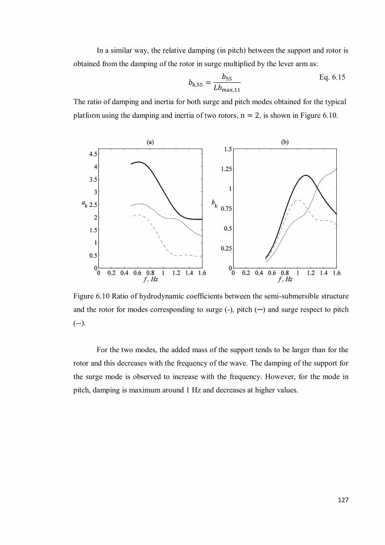
127
In a similar way, the relative damping (in pitch) between the support and rotor is
obtained from the damping of the rotor in surge multiplied by the lever arm as:
𝑏k,55 =
𝑏55𝐿𝑏max,11
Eq. 6.15
The ratio of damping and inertia for both surge and pitch modes obtained for the typical
platform using the damping and inertia of two rotors, n = 2, is shown in Figure 6.10.
Figure 6.10 Ratio of hydrodynamic coefficients between the semi-submersible structure
and the rotor for modes corresponding to surge (-), pitch (─) and surge respect to pitch
(--).
For the two modes, the added mass of the support tends to be larger than for the
rotor and this decreases with the frequency of the wave. The damping of the support for
the surge mode is observed to increase with the frequency. However, for the mode in
pitch, damping is maximum around 1 Hz and decreases at higher values.

128
6.9 Single Mode Response: Surge Only
The objective of this section is to identify a combination of support-structure parameters
– forcing, added mass and damping – that mitigate peak rotor loads compared to a rigid
support. The approach taken is to characterise the contribution of structure dynamics to
the extreme loads experienced by the rotor with the range of damping, mass of support
and ratio of forces analysed in Sections 6.6, 6.7 and 6.8. Initially motion in surge only is
considered (mode j=1 in Eq. 6.2). The time-varying response of the rotor motion, 𝑥1, is
obtained and the corresponding force (𝐹osc) is then analysed for the peak force applied to
the dynamically responding rotor. The equation of motion for response in surge only is:
𝑋1+𝑋e,1 + n (𝐹I,11(�̈�1, �̇�0, �̇�wave,p) + 𝐹D,11(�̇�1, 𝑢0, 𝑢wave,p))
= (𝑚11 + 𝑎11 + n𝑚rotor,11)�̈�1+𝑏11�̇�1 + 𝑘11𝑥1
Eq. 6.16
The extreme force imposed on the rotor due to dynamic response is obtained
using the process of Section 4.7, by superposing the maximum force due to relative
velocity, mean flow and turbulence alone, 𝐹′1n. The extreme force is made proportional to
the mean thrust of the dynamic response, �̅� and written as:
𝐹1n,dynamic
�̅�= [
𝐹osc,max�̅�
] +𝐹′1n�̅�
Eq. 6.17
The influence of the structure dynamics on the extreme support loads is described
by the ratio of extreme forces imposed on a rotor supported on a stiff tower and subjected
to the same operating flow, which consists of a turbulent flow combined with opposing
waves. A ratio between peak force on the flexible and rigid supports is calculated from
Eq. 4.17 and Eq. 6.17 as:
𝐹Κ =𝐹1n,dynamic
𝐹1n,rigid
=𝐹osc,max + 𝐹′1
n
n (𝐹0 + 𝐹′1n+ 12 𝜌𝐴𝐶D‖𝑢wave,p‖(𝑢0 + ‖𝑢wave,p‖) + 𝑋e,1)
Eq. 6.18
The procedure to obtain rotor response and force is as follows. Initially, the
dynamic force on each rotor due to sum contribution of the drag and added mass is
rewritten from Eq. 2.39 and Eq. 2.47 as:

129
𝐹D,11(�̇�1, 𝑢0, 𝑢wave,p) + 𝐹I,11(�̈�1, �̇�0, �̇�wave,p)
=12𝜌𝐴𝐶D
(𝑢0 + 𝑢wave,p − �̇�1)|𝑢0 + 𝑢wave,p − �̇�1|
+ 𝜌𝑉𝐶′a(�̇�0 + �̇�wave,p − �̈�1) + 𝜌𝑉�̇�wave,p
Eq. 6.19
Since the added mass force of a rotor in the turbulent channel flow is typically
small compared to the drag force (see Section 4.5), the added mass component is
simplified as
𝜌𝑉𝐶′a(�̇�0 + �̇�wave,p − �̈�1) ≈ −𝜌𝑉𝐶′a�̈�1 Eq. 6.20
and so inertia force is
𝐹I,11(�̈�1, �̇�0, �̇�wave,p) = −𝜌𝑉𝐶′a�̈�1 + 𝜌𝑉�̇�wave,p Eq. 6.21
Rewriting only the drag force in Eq. 6.19, and by treating the drag due to the mean
current velocity separate to drag due to relative velocity associated with waves and rotor
motion, the force applied per rotor is:
𝐹D,11(�̇�, 𝑢0, 𝑢wave,p)
=12𝜌𝐴𝐶D,1𝑢0
|𝑢0 + 𝑢wave,p − �̇�1|
+12𝜌𝐴𝐶D,2
(𝑢wave,p − �̇�1)|𝑢0 + 𝑢wave,p − �̇�1|
Eq. 6.22
Assuming that the mean flow is much greater than the maximum of the net
velocity due to wave-induced flow and rotor oscillation, the first term in Eq. 6.22 is
approximated as: 12𝜌𝐴𝐶D,1𝑢0
|𝑢0 + 𝑢wave,p − �̇�1| =12𝜌𝐴𝐶D,1
(𝑢02 + 𝑢0𝑢wave,p − 𝑢0�̇�1) Eq. 6.23
For the range of wave velocities and rotor velocities modelled, drag force is
dominated by terms dependent on the mean flow (𝑢02), thus 𝐶D,1 = 𝐶T . Neglecting the
terms 𝑢0𝑢wave,p(𝑥1, 𝑡) − 𝑢0�̇�1 the force is:
12𝜌𝐴𝐶D,1
(𝑢02 + 𝑢0𝑢wave,p − 𝑢0�̇�1) ≈ 𝐹0 Eq. 6.24
The dynamic force of the rotor is hence reduced to the rotor thrust when supported
on a stiff support in a mean flow superposed with a force due to the rotor motion within
an incident mean flow with waves:
𝐹D,11(�̇�1, 𝑢0, 𝑢wave,p) = 𝐹0 +12𝜌𝐴𝐶D,2
(𝑢wave,p − �̇�1)|𝑢0 + 𝑢wave,p − �̇�1| Eq. 6.25

130
Herein, the second drag is analogous to the drag coefficient due to the oscillatory
flow, thus 𝐶D,2 ≈ 𝐶D (see Section 4.6, Eq. 4.9). After substituting Eq. 6.21 and Eq. 6.25
into Eq. 6.16, the equation of motion for motion in surge only is:
(𝑚11 + 𝑎11+n𝑚rotor,11+n𝜌𝑉𝐶′a)�̈�1+𝑏11�̇�1 + 𝑘11𝑥1 Eq. 6.26
= 𝑋1 + 0.08𝐹0
+n (12𝜌𝐴𝐶D(𝑢wave,p − �̇�1)|𝑢0 + 𝑢wave,p − �̇�1| + 𝐹0)
+n𝜌𝑉�̇�wave,p
It can be seen that to reduce the thrust fluctuations relative to a rigid support, the
drag force resulting from the streamwise oscillation and waves should be out of phase
with the wave forcing due to the support. This is to ensure that the right hand side terms
of, 𝑋1 + n𝐹D,11, are minimised. The drag force 𝐹D,11 is mainly due to wave induced
horizontal velocity and is in phase with the surface elevation.
To obtain predictions of thrust and response amplitude, the equation of motion
(Eq. 6.26) is initially transformed into a set of first-order differential equations (ODE). A
solution is then provided in a forward time scheme by a numerical solver. Here, the
Matlab solver ODE45 based on the Runge Kutta method is employed. The solution
procedure begins by setting the differential equations as:
𝑑𝑑𝑡[𝑥�̇�] =
𝑑𝑑𝑡[𝑋] = finitial
Eq. 6.27
where 𝑋 is the matrix of the set of differential equations and finitial, the initial
conditions. The conditions are initially set to zero, until a steady periodic solution is
reached. The acceleration is then isolated from Eq. 6.26 and substituted into Eq. 6.27 so
that the set of differential equations becomes:
𝑑𝑑𝑡 [
𝑥1�̇�1]
= [�̇�1
𝑋e,1 + 𝑋1 + n𝐹D,11(�̇�1, 𝑢0, 𝑢wave,p) + n𝜌𝑉�̇�wave,p − 𝑘11𝑥1 − 𝑏11�̇�1𝑚11 + 𝑎11 + n𝑚rotor,11 + n𝜌𝑉𝐶′a
]
= finitial
Eq. 6.28
The main advantage of a time domain compared to a frequency model is the
allowance of synthetic incident velocities of the combined wave and channel flows. This
approach would also allow, at a later date, implementation of non-linear effects such as
more realistic mooring lines and wave drift forces.
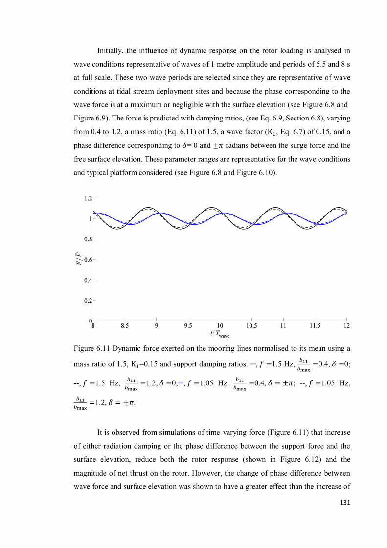
131
Initially, the influence of dynamic response on the rotor loading is analysed in
wave conditions representative of waves of 1 metre amplitude and periods of 5.5 and 8 s
at full scale. These two wave periods are selected since they are representative of wave
conditions at tidal stream deployment sites and because the phase corresponding to the
wave force is at a maximum or negligible with the surface elevation (see Figure 6.8 and
Figure 6.9). The force is predicted with damping ratios, (see Eq. 6.9, Section 6.8), varying
from 0.4 to 1.2, a mass ratio (Eq. 6.11) of 1.5, a wave factor (K1, Eq. 6.7) of 0.15, and a
phase difference corresponding to 𝛿= 0 and ±𝜋 radians between the surge force and the
free surface elevation. These parameter ranges are representative for the wave conditions
and typical platform considered (see Figure 6.8 and Figure 6.10).
Figure 6.11 Dynamic force exerted on the mooring lines normalised to its mean using a
mass ratio of 1.5, K1=0.15 and support damping ratios. ─, 𝑓 =1.5 Hz, 𝑏11𝑏max
=0.4, 𝛿 =0;
--, 𝑓 =1.5 Hz, 𝑏11𝑏max
=1.2, 𝛿 =0;─, 𝑓 =1.05 Hz, 𝑏11𝑏max
=0.4, 𝛿 = ±𝜋; --, 𝑓 =1.05 Hz,
𝑏11𝑏max
=1.2, 𝛿 = ±𝜋.
It is observed from simulations of time-varying force (Figure 6.11) that increase
of either radiation damping or the phase difference between the support force and the
surface elevation, reduce both the rotor response (shown in Figure 6.12) and the
magnitude of net thrust on the rotor. However, the change of phase difference between
wave force and surface elevation was shown to have a greater effect than the increase of

132
damping of the support platform. The least and most favourable phase of the force support
was obtained at 0 and close to ±𝜋 radians. The support-structure response has negligible
effect on the mean force for all cases.
Figure 6.12 Linear displacement in a support unconstrained to surge using representative
damping, mass and force ratios. Line styles as Figure 6.11.
To identify support-structure characteristics (excitation force, radiation damping,
added mass and stiffness) that reduce the extreme loading, peak forces (1 in 100) were
obtained for the studied flexible support (see Section 6.7). Three amplitudes of support
platform forces were studied, both without and with a phase difference to surface elevatio.
The 1 in 100 forces obtained with force in phase with surface elevation (𝑓 =1.5 Hz) for
a platform supporting a single rotor are shown in Figure 6.13. Figure 6.14 shows the 1 in
100 forces for the same platform supporting two rotors for the same wave condition. For
a single rotor, the dynamic response resulted in extreme loading almost equal or greater
than that experienced by a rotor with a rigid support. Increasing the amplitude of the wave
force was found to increase the extreme force. However, for multiple rotors on a single
structure the additional damping leads to a reduction of the extreme forces by up to 4%
in comparison to a single rotor on a rigid support (Figure 6.14a).
For the lower wave frequency (𝑓 =1.05 Hz) the ratio of extreme support forces
were reduced by up to 12 % for both single- and two-turbine case (see Figure 6.15 and
Figure 6.16). This greater reduction is due to the phase difference between the force and

133
surface elevation. The influence of peak loading with increasing or reducing mass of the
support was observed to be small.
Figure 6.13 Extreme forces with 1% probability of exceedance on one rotor supported
from a floating structure relative to same forces on a rigid structure. a) K1 =0.1. b)
K1 =0.2. c) K1 =0.3. 𝑓 =1.5 Hz, 𝛿 =0 for all cases.

134
Figure 6.14 Extreme forces with 1% probability of exceedance on one of two rotors
supported from a floating structure relative to same forces on a rigid structure. a) K1 =0.1.
b) K1 =0.2. c) K1 =0.3. 𝑓 =1.5 Hz, 𝛿 =0 for all cases.
Figure 6.15 Extreme forces with 1% probability of exceedance on one rotor supported
from a floating structure relative to same forces on a rigid structure. a) Wave factor
K1 =0.1. b) K1 =0.2. c) K1 =0.3. 𝑓 = 1.05 Hz, 𝛿 = ±𝜋 for all cases.

135
Figure 6.16 Extreme forces with 1% probability of exceedance on one of two rotors
supported from a floating structure relative to same forces on a rigid structure. a) K1 =0.1.
b) K1 =0.2. c) K1 = 0.3.𝑓 =1.05 Hz, 𝛿 = ±𝜋 for all cases.
The dynamic response of a floating support platform can thus reduce peak loads
on a rotor under several conditions: if the amplitude of wave-induced forces is less than
the rotor dynamic peak thrust, K1<0.2, if the phase between the wave force and surface
elevation is close to ±𝜋 radians, if more than one rotor is supported on the same platform,
or if net damping associated with the supporting platform is greater than that of the
averaged rotor. However, the greatest reduction of extreme force was obtained when the
relative phase between the wave force and surface elevation is approaching to an anti-
phase condition. The extreme forces obtained for the frequency condition with 𝛿 = ±𝜋
using either one or two rotors were mostly reduced in comparison to a rigid platform.
This applied for the range of damping and mass ratios considered. For a particular
platform geometry, the phase of the force relative to elevation is related to the wavelength,
hence a function of the wave frequency and therefore forcing in anti-phase to elevation
would be limited to a narrow range of frequencies.

136
6.10 Coupled Pitch and Surge
A coupled model of the pitch and surge response of the supporting platform is employed
to investigate the extreme load variation of the platform concept in the same
representative turbulent and oscillatory flow condition. Pitch and surge of the platform
define the motion of the rotor in surge only. Rearranging Eq. 6.2 for the surge and pitch
coupled motion (j=1,5), the equation of motion of the support structure becomes:
(𝑚11 + 𝑎11 + n𝑚rotor,11)�̈�1 + 𝑏11�̇�1+𝑘11𝑥1 + 𝑎15�̈�5 + 𝑏15�̇�5= n0.08𝐹0 + 𝑋1+ n𝐹D,11(�̇�rotor,1, 𝑢c, 𝑢wave,p)+n𝐹I,11(�̈�rotor,1, �̇�c, �̇�wave,p)
+n𝐹D,15(�̇�rotor,5, 𝑢c, 𝑢wave,p)+n𝐹I,15(�̈�rotor,5, �̇�c, �̇�wave,p)
Eq. 6.29
Defining surge of the rotor in terms of pitch and surge of the support:
(𝑚11 + 𝑎11 + n𝑚rotor,11)�̈�1 + 𝑏11�̇�1+𝑘11𝑥1 + 𝑎15�̈�5 + 𝑏15�̇�5= n0.08𝐹0 + 𝑋1+ n𝐹D,11(�̇�1, 𝑢c, 𝑢wave,p)+n𝐹I,11(�̈�1, �̇�c, �̇�wave,p)
+ n𝐹D,11(�̇�5𝐿, 𝑢c, 𝑢wave,p)+n𝐹I,11(�̈�5𝐿, �̇�c, �̇�wave,p)
Eq. 6.30
The contribution of drag and inertia of each rotor in surge motion is written as
shown in Section 6.9. The time-dependent pitch equation of motion is obtained similarly
to the surge by employing Eq. 6.3 with the parameters set to j=1,5 and approximating the
rotor displacements with support motion as:
(𝑚55 + 𝑎55 + n𝑚rotor,11𝐿2)�̈�5 + 𝑏55�̇�5+𝑐55𝑥5 + 𝑎51�̈�1 + 𝑏51�̇�1= n0.08𝐹0𝐿 + 𝑋5+ n𝐹D,11(�̇�5𝐿, 𝑢c, 𝑢wave,p)𝐿 + n𝐹I,11(�̈�5𝐿, �̇�c, �̇�wave,p)𝐿
+ n𝐹D,11(�̇�1, 𝑢c, 𝑢wave,p)𝐿+n𝐹I,11(�̈�1, �̇�c, �̇�wave,p)𝐿
Eq. 6.31
The predictions of thrust and response amplitude of oscillation are obtained by the
time-domain solution of the set of first-order differential equations of pitch and surge
motion ( Eq. 6.29 and Eq. 6.31 ) as shown in Section 6.9. The implementation and
conversion of the force formulas into a set of ODE is shown in Appendix C.
The dynamic displacement and force on the rotor due to coupled surge and pitch
of the support was contrasted to the force on a rigid structure as Eq. 6.18, Figure 6.16,
Section 6.9. The time-varying force per rotor supported on a stiff tower due to mean
current, waves and response (see Eq. 5.5 and Eq. 6.18) is:
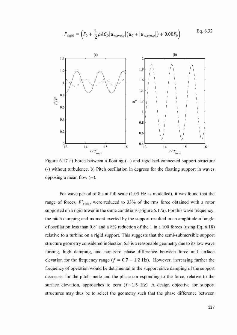
137
𝐹rigid = (𝐹0 + 12 𝜌𝐴𝐶D
|𝑢wave,p|(𝑢0 + |𝑢wave,p|) + 0.08𝐹0) Eq. 6.32
Figure 6.17 a) Force between a floating (--) and rigid-bed-connected support structure
(-) without turbulence. b) Pitch oscillation in degrees for the floating support in waves
opposing a mean flow (--).
For wave period of 8 s at full-scale (1.05 Hz as modelled), it was found that the
range of forces, 𝐹′rms, were reduced to 33% of the rms force obtained with a rotor
supported on a rigid tower in the same conditions (Figure 6.17a). For this wave frequency,
the pitch damping and moment exerted by the support resulted in an amplitude of angle
of oscillation less than 0.8˚ and a 8% reduction of the 1 in a 100 forces (using Eq. 6.18)
relative to a turbine on a rigid support. This suggests that the semi-submersible support
structure geometry considered in Section 6.5 is a reasonable geometry due to its low wave
forcing, high damping, and non-zero phase difference between force and surface
elevation for the frequency range (𝑓 = 0.7 − 1.2 Hz). However, increasing further the
frequency of operation would be detrimental to the support since damping of the support
decreases for the pitch mode and the phase corresponding to the force, relative to the
surface elevation, approaches to zero (𝑓~1.5 Hz). A design objective for support
structures may thus be to select the geometry such that the phase difference between

138
wave-excitation force and wave-induced velocity is maximum whilst wave amplitude
large.
6.11 Summary
Floating support structures for wind and tidal stream turbines were reviewed. The
influence of loading and response on rotor loading was identified as a design uncertainty.
In this chapter the dynamic response of a rotor rigidly connected to a floating support is
analysed based on the response in surge and pitch of a floating support rigidly connected
to a turbine. A semi-submersible geometry studied by Van der Plas (2014) and Francis
and Hamilton (2007) is simplified to a slender half-cylinder. Wave forcing, added mass
and radiation damping are obtained from the diffraction code WAMITTM. The external
constraint of a mooring line was modelled as a low stiffness spring. Forcing on the rotor
was defined by the mean incident flow, waves and streamwise motion of the rotor as per
the analysis of Chapter 4.
The effect of dynamic response on the mean, variance and peak values of rotor
loading was investigated due to response in two modes: independent pitch and coupled
surge and pitch and for a range of hydrodynamic coefficients, wave forces and moments.
Two wave frequencies were considered with phase difference between the support
platform wave force and surface elevation close to 0 and ±𝜋 radians. For these wave
frequencies, peak thrust was reduced compared to a rigid support structure when the phase
difference was ±𝜋 radians. Force was also reduced when the phase difference was zero
if the following conditions were met: multiple rotors, net damping coefficients of at least
equivalent to the rotor damping and amplitude of wave forces, K1, below 0.2 of the
dynamic rotor thrust. The extreme thrust per turbine was found to be lower for a structure
supporting two rotors due to the additional damping of the rotor. For the wave condition
with phase difference, the 1 in 100 exceedance force for motion in surge was found to
reduce across the range of achievable hydrodynamic parameters (added mass and
damping) of the support by up to 12% relative to a rotor supported on a rigid tower.
For the simplified support structure geometry modelled, the 1 in 100 exceedance
force for motion in coupled surge and pitch was found to reduce by approximately 8%

139
due to structure dynamics when compared to the rotor response obtained from a stiff
support structure.

140
CHAPTER 7: CONCLUSIONS
The overall aim of the thesis was to determine how the response of a floating support
platform affects the loading of wind or tidal stream turbines. The particular interest was
the influence of the dynamic response on the occurrence and magnitude of the maximum
loads applied to the rotor of a tidal stream turbine during operation since these loads
directly influence tidal system design.
It was found that the support-structure dynamics can either increase or reduce the
extreme thrust of the turbine relative to the rotor response on a rigid structure, and this
was dependent on the hydrodynamic damping, added mass and excitation force on the
supporting platform at particular wave frequencies. A support-platform geometry that
minimises peak forces on the rotor would be characterised by low wave forcing, a
damping of at least equivalent to the rotor and an excitation force in anti-phase to the
surface elevation. Due to the multiple wave frequencies encountered in sea states, the
magnitude of the phase force from the support would then be optimised for the most
representative frequency of flow operation.
To model loading coupled with response, the loading on a horizontal-axis rotor
has been investigated as it responds to different types of onset flow representing the flows
experienced by a rotor during operation. These included the mean and time-varying rotor
loads due to an incident uniform flow, a turbulent channel flow, oscillatory incident flow
due to waves opposing turbulent flow and due to sinusoidal oscillation of the rotor within
quiescent flow and turbulent flow. The understanding of each effect on the turbine’s
performance was investigated using engineering tools such as BEMT and by
experimental investigation of time variation of rotor thrust in turbulent channel flows,
oscillatory flow and due to oscillation relative to a mean flow. The loading in turbulent
channel flow was acquired from the variance of the rotor thrust measurements and related
to the standard deviation of the operating-flow velocities. The thrust and power curves
modelled with the BEMT model was obtained within 10% of the mean measured rotor
performance in an operating flow with 𝑇𝐼 =12%.
Forces with probability of occurrence 1 in 100 (1%) in the mean flow with
turbulence present (𝑇𝐼 =12%) were around 140% of the mean thrust. The variation of
extreme loads due to mean flow combined with turbulence and opposing waves was
investigated and approximated with a Morison equation (Eq. 4.9) by ignoring inertia

141
coefficient and accounting for the mean loading due to uniform flow, as well as the
turbulent thrust fluctuations and the wave loading. The effect of waves on the rotor
loading was found to increase the extreme loading as a function of relative velocity using
a drag coefficient of 2 and the mean force was close to the value in turbulent channel
flow.
For the wave conditions applicable to rotor operation at full scale (typically less
than 3m wave height) the maximum 1% force encountered was approximately 190% of
the mean thrust. The damping coefficient of a disc (using Eq. 4.5) of similar rotor thrust
increased linearly with the amplitude of streamwise oscillation, 𝐾𝐶, and the magnitude
of the slope using a least-squares approach was approx. 0.15. The added mass coefficient
was found to be small in comparison to the damping in all conditions studied, with
magnitude approximately 0.12.
The dynamic force on a support structure was considered as a combination of the
loading on the turbine due to turbulent flow and waves, loading of the turbine due to
response and the direct loading on the immersed part of the supporting platform.
Subsequently, the influence of the structure dynamics on the rotor thrust was analysed
using wave forcing by linear analysis in an uncoupled surge-pitch structure model with
the mechanical properties of the support defined as proportional to the rotor. Two wave
conditions were studied with phase difference between the wave force support and the
surface elevation of zero and ±𝜋 radians. It was found that extreme forces were reduced
relative to a rigid support if the force phase difference was close to ±𝜋 radians. When this
condition is not met, extreme forces can be reduced in the following conditions: multiple
rotors, surge and pitch damping coefficients of at least the same of the rotor and with
amplitudes of support forces being lower than 0.2 of the peak rotor thrust imposed in
forced axial oscillations. The dynamic response applied to a typical support platform
geometry due to mean flow and with wave forcing on the platform close to anti-phase
with surface elevation exhibited a reduction of peak rotor force (1 in a 100) by about 8%
in comparison to rotor response on a rigid bed-mounted support. The findings of rotor
thrust and support structure influence are summarised below.
142
Mean and variance of thrust
A BEM numerical model based on wind rotor loading was shown to be suitable for the
prediction of thrust and power output from a tidal stream turbine due to a steady flow.
This method was evaluated against predictions for a 0.27 m rotor and a new set of
experimental measurements in a mean flow with 𝑇𝐼 =12%. Evaluation was also
conducted using published performance data for two tidal stream turbines of a 0.8 metre
rotor diameter each (Batten et al., 2008; Galloway et al., 2011). The blockage effects on
the experiments using the 0.27 m single rotor were corrected using a wind-tunnel method
and found negligible for the steady-flow coefficients of thrust and power.
The thrust fluctuations normalised to the mean in the turbulent channel flows were
found to increase proportionally to the turbulence intensity that is averaged across the
rotor. A multiplier (admittance) factor, 𝐾I, which relates the intensity of fluctuations
(standard deviation over mean) between the thrust and hub-height velocity for flows
corresponding to a 𝑇𝐼 =12% and 𝑇𝐼 =14% was obtained as 1.17 and 1.5. The measured
thrust fluctuations in the turbulent channel flows were predicted using an aerodynamic
admittance previously obtained for square plates in grid-generated turbulence. The
comparison between the measurements and predictions were considered to be good due
to the discrepancy of the object (rectangular plate rather than rotor) and the operating
flows (grid against open channel turbulence) employed between the theoretical model and
experiments.
For a single rotor, the time-average thrust obtained due to forced streamwise
oscillations within a turbulent channel flow of 𝑇𝐼 =12% remained within 7% of the mean
thrust that is imposed when the rotor is supported on a stiff tower and subjected to
turbulent channel flows of 𝑇𝐼 =12% and 𝑇𝐼 =14% and in eighteen wave conditions
opposing a turbulent channel flow of 𝑇𝐼 =12%.
Turbine Hydrodynamics
The damping of a porous disc (Eq. 4.5) oscillating in quiescent flow was a linear function
Keulegan Carpenter number, 𝐾𝐶. The drag coefficient of the disc (using Eq. 2.39) was
found to decay exponentially with 𝐾𝐶 to a limiting value of 2 for 𝐾𝐶 > 1. A drag term
was evaluated against measurements of force due to streamwise oscillation within

143
turbulent flows by summing the mean thrust due to turbulent channel flow with a drag
force due to streamwise oscillation about the mean velocity (Eq. 4.9, approach based on
Eq. 2.49). The drag coefficient obtained for a disc and rotor oscillating in incident
turbulent channel flows was found to be comparable. The drag coefficient on a disc in
turbulent channel flow was within 6% of the drag obtained for a porous disc forced to
oscillate in quiescent flow. The accuracy of the drag assumption was limited to 𝐾𝐶 <
0.65. The discrepancy was attributed to the approximation of the relative velocity
between the water and disc and the neglected terms in the modified Morison force
associated with turbulent fluctuations. The added mass for the disc and rotor in quiescent
and turbulent channel flows was approximately constant with 𝐾𝐶 and the magnitude was
approximately 12% of the virtual mass predicted for a non-perforated disc (defined by a
spheroid) using potential flow theory. The effects of added mass were much lower than
drag and these were found to be negligible when considering maximum rotor loading.
Extreme loading
The magnitude of the thrust on a rotor in turbulent channel flow exceeded by 1%, 0.1%
and 0.01% samples was analysed using the peak-over-threshold technique with the Type
1 distribution and Pareto tail-fitting technique. The 0.01% force in turbulent channel flow
only and in mean flow combined with turbulence and waves can be considered
representative of the loading occurring on a full-scale turbine on average once every two
days when operating in similar flow. Threshold magnitudes of 1.25 and 1.1 times the
mean force were selected for the loading due to oscillatory and turbulent channel flows.
A 10 minute sample measurement was found to obtain the extremes using Type 1
distribution within 3% from 30 min sample of the experimental measurement of force in
turbulent channel flow and from 44 min sample of the experimental measurement of force
due to turbulence channel flow with opposing waves. The 1% force was 1.38 and 1.59
times the mean thrust corresponding to the flow conditions with 𝑇𝐼 =12% and 𝑇𝐼 =14%.
The prediction of loads was also analysed in terms of sample length and threshold forces
by using Type 1, Normal and Weibull distributions and these provided similar extremes
within 3%.
In waves opposing a turbulent channel flow, the maximum 0.01% force
encountered was acquired with waves specified as 0.7 Hz and 20mm with a magnitude of
144
2.36 times the mean thrust. The extreme forces in the oscillatory flow conditions
increased quadratically with the amplitude of wave velocity and as amplitude of velocity
decreased, the initial thrust was comparable to the turbulent channel flow of 𝑇𝐼 = 12%.
The spectrum of the excitation force in the combined flow with small wave height was
comparable to the force superposition of the ambient and wave frequency load.
A Morison equation was evaluated against the extreme force measurements in
small waves by summing the load deviation in turbulent channel flow with a wave-
induced force (Eq. 5.1, approach based on Eq. 2.48). Linear wave theory provided the
measured velocity at hub height to within 7% for a range of wave conditions. Definition
of the drag associated with wave induced velocity in terms of the square of wave velocity
provides extreme force as (Eq. 5.2):
𝐹1n,wave
=12𝜌𝐶D,wave𝜋𝑅
2‖𝑢wave‖2
For this drag model, a thrust coefficient of 0.89 in the turbulent channel flow and
drag coefficient of magnitude 11 for the wave conditions were attained. The simulated
extreme force curves had initial values comparable to the exceedance load in turbulent
channel flow and increased exponentially with the amplitude of the wave velocity. The
extreme forces were predicted within 8% by employing linear wave prediction of
velocity.
A force prediction method (approach based on Eq. 4.9) using relative velocity at
hub height, defined by the product of wave velocity and wave velocity superposed with
mean flow, and a drag coefficient of 2 was evaluated to obtain the extremes in forced
streamwise motion tests in a turbulent channel flow. Definition of the drag force
associated with the wave-induced velocity is (Eq. 5.5): 12𝜌𝐴𝐶D,wave𝑢wave,p
|𝑢0 − 𝑢wave,p| = 𝐹osc,p
For this formulation the extreme forces were predicted to within 6% and
asymptote to a limit as the wave velocity increases relative to the mean flow. This
discrepancy is within the 7% difference between measured hub height velocity and
velocity predicted by linear wave theory providing confidence in this approach for peak
force prediction. This method also provides a reasonable prediction of the time-varying
force due to waves with turbulence.

145
Effect of platform response on extreme loading
Dynamic response of a floating platform was considered in pitch and surge modes due to
forcing on the turbine associated with uniform flow, turbulence, waves and streamwise
oscillation of the rotor due to the response of the support structure the forcing of which is
obtained by linear diffraction theory. The dynamic response in the time-dependent pitch
and surge motion was studied for a typical floating platform geometry.
The simulations of dynamic response in uncoupled surge and pitch modes
exhibited a reduction of the extreme loads in specific circumstances. This included when
the phase magnitudes between the surface elevation and support force were close to ±𝜋
radians. In the condition without phase difference, greatest reduction of rotor force was
achieved using multiple rotor devices in a support that produces low wave force
amplitudes between support and rotor. Support platform force amplitudes of less than
20% of the mean rotor force and damping coefficients in surge and pitch of at least equal
to the rotor damping reduced extreme force on the rotor. It was found that a phase
difference between the wave force and the hub velocity caused cancellation of rotor drag
with the wave support force and thus extremes forces with 1% probability of exceedance
were reduced by up to 12% for motion in surge only.
This geometry was found beneficial by imparting low wave-support responses,
damping coefficients of support over rotor plane between 0.2-1.25 and phase magnitudes
close to ±𝜋 radians for the range of frequencies (0.7-1.2 Hz). These properties applied to
a scaled floating moored platform in a wave condition with support forcing close to anti-
phase with the surface elevation showed an 8% reduction of the peak load (probability of
occurrence 1 in a 100) for motion in coupled pitch and surge, when compared to that
acquired in a bed-mounted support.

146
Recommendations for future work
The last section concerns more research to be performed to further improve understanding
of the dynamic performance of the rotor and the support in flow conditions representative
of tidal stream sites. This includes the assessment, prediction and evaluation of the
floating system response, the coupled mooring lines, the rotor performance and the
solution of the time-dependent model of the floating system in 3 or more coupled degrees
of freedom. These suggestions may be relevant for future investigation of cost-effective
supports to be utilised in deep water.
Loading in Turbulent Channel flow Only
Extreme forces are expected to play a crucial role in capital costs of any support design
and rotor force fluctuations were found to increase with the flow’s turbulent intensity.
However, the deployment of multiple devices is required for its feasible
commercialisation and the array itself influence the local incident flow and hence turbine
operation. Therefore, various aspects are encouraged such as the study of extreme forces
due to array configurations at different lateral and downstream spacing, the change of
thrust caused by channel blockage and evaluation of thrust coefficient against onset local
flow standard deviations. Differences and advantages of rotor operation with constant
torque and constant speed are also important to further address by using engineering
methods such as the BEMT, Morison-based equations and experimental measurements.
Loading due to Waves and Turbulent Channel Flow
The work presented in the thesis was limited to flow conditions, which were propagated
perpendicularly to the rotor swept area. Turbine design and the wide range of flow
directions that occur at some tidal stream sites may require yawed operation for part of
the cycle. In addition, waves are likely to be irregular with variation of dominant
direction. To improve understanding of rotor loading in oblique waves and yawed onset
flow, a set of experiments would be required to evaluate performance of the rotor in
incident flows and irregular waves misaligned to rotor axis. Alternatively, this
experimental study may be attained in another wave flume facility by generating wave

147
conditions at different propagation angles relative to the mean flow. This finding as an
input to coupled rotor response leading to multi-mode response in a floating moored
platform is relevant for the design and innovation of dynamic support systems. Such
information may be used to produce guidelines to cover aspects such as rotor device
performance and detailed optimisation of rigid support structures in indicative tidal
stream sites.
Loading due to Forced Streamwise Motion
The loading due to forced streamwise motion was investigated in perpendicular quiescent
and turbulent channel flows to the rotor and the results were used as input to a model of
structural dynamics. Coupled pitch and surge sinusoidal motion of the support platform
were regarded as contributing to most of the rotor’s variation of thrust. This result may
be considered for ideal operating conditions, whereby the incoming waves are
monochromatic and decay effects are small. This leads to some uncertainties of dynamic
response in irregular motion and in oblique waves combined with current flows. Hence,
proper tools must be first developed to understand uncoupled rotor behaviour in order to
combine into a structure response model. This will require the design of stiffer oscillating
support equipment to induce the total contribution of sinusoidal rotor displacement in
mean flow with turbulence present and in same flow combined with waves of different
directions, amplitude and wave peak frequencies. The new damping and drag parameters
as a function of 𝐾𝐶 would provide a broader understanding of wave-current interactions
and demonstrate key differences between rotor operation with and without forced
streamwise motion.
Hydrodynamic Coefficients of the Rotor
Most of the floating supports that have been proposed are comprised of a pair of rotors so
that their own thrust aligns to the incident flow and counteracts the yaw moment applied
to the immersed support. Nevertheless, the yaw moment induced by the rotor in
misaligned flow conditions may be large relative to the floating support. The decoupling
effect of the rotor could be further explored by quantifying the rotor hydrodynamics in
additional degrees of freedom such as yaw, and heave. The resulting coupled predicted

148
motion between the turbine and platform would serve as a basis design of the mooring
lines to keep system's oscillations within acceptable operation. Various aspects of
mooring representations such as linear spring forces and dynamic analyses have been
included for floating wind-turbine platforms (Qiao and Ou, 2014) to reduce the surge,
heave and yaw induced moments (Nielsen et al., 2006; Skaare et al., 2007). Therefore, a
similar approach for tidal floating supports should be appraised to limit the system’s
oscillations and protect against extreme conditions.
Alternative Support Structures
There is substantial work to be done to assess the cost-benefits of each support system,
which are appropriate for the site characteristics, the rotor employed (wind or tidal) and
the mooring system preferred. Hydrodynamic interactions and influence of rotor loading
can be investigated using representative dimensions and linear wave forcing of support
structure such as Tension Leg Platforms, spar systems and semi-submersible concepts.
The influence of the dynamic structure can be expanded into an equation of motion to
include time-dependant hydrodynamics and drift forces of the support, as well as non-
linear interaction of the mooring lines and hydrodynamics of the rotor in surge, pitch and
yaw motion.
Evaluation of Dynamic response
A set of experiments on simple buoy and scaled support devices in turbulent channel flow
combined with waves will be needed to quantify the moments and the hydrodynamic
coefficients as well as to evaluate the suitability of WAMITTM. Prediction methods of the
moored dynamic support will be validated against measurements. This study will lead to
the development of a fully coupled model for the design, and the assessment of life
support and improvement of the current marine offshore platforms technology.

149
References
ABPmer, The Met Office & Proudman Oceanographic Laboratory (2004), "Atlas of UK Marine Renewable Energy Resources". Technical report R.1106, September 2004. Afgan I., McNaughton, J., Rolfo, S., Apsley, D., Stallard, T., and Stansby, P. (2013), "Turbulent Flow and Loading on a Tidal Stream Turbine by LES and RANS", International Journal of Heat and Fluid Flow, 43, 96-108. An, S., and Faltinsen, O. M. (2013), "An Experimental and Numerical Study of Heave Added Mass and Damping of Horizontally Submerged and Perforated Rectangular Plates", Journal of Fluids and Structures, 39, 87-101. Atlantis Resources Ltd. URL http://atlantisresourcesltd.com/ Bahaj, A., Myers, L., Rawlinson-Smith, R., and Thomson, M. (2012), "The Effect of Boundary Proximity Upon the Wake Structure of Horizontal Axis Marine Current Turbines", Journal of Offshore Mechanics and Arctic Engineering, 134, 021104. Bahaj, A. S., Batten, W. M. J., and McCann, G. (2007), "Experimental Verifications of Numerical Predictions for the Hydrodynamic Performance of Horizontal Axis Marine Current Turbines", Renewable Energy, 32, 2479-2490. Bahaj, A. S., Molland, A. F., Chaplin, J. R., and Batten, W. M. J. (2007), "Power and Thrust Measurements of Marine Current Turbines under Various Hydrodynamic Flow Conditions in a Cavitation Tunnel and a Towing Tank", Renewable Energy, 32, 407-426. Barltrop, N., Varyani, K. S., Grant, A., Clelland, D., and Pham, X. P. (2007), "Investigation into Wave-Current Interactions in Marine Current Turbines", Proceedings of the Institution of Mechanical Engineers, Part A: Journal of Power and Energy, 221, 233-242. Batten, W. M., Harrison, M., and Bahaj, A. (2013), "Accuracy of the Actuator Disc-Rans Approach for Predicting the Performance and Wake of Tidal Turbines", Philosophical Transactions of the Royal Society A: Mathematical, Physical and Engineering Sciences, 371, 20120293. Batten, W. M. J., Bahaj, A. S., Molland, A. F., and Chaplin, J. R. (2007), "Experimentally Validated Numerical Method for the Hydrodynamic Design of Horizontal Axis Tidal Turbines", Ocean Engineering, 34, 1013-1020. Batten, W. M. J., Bahaj, A. S., Molland, A. F., and Chaplin, J. R. (2008), "The Prediction of the Hydrodynamic Performance of Marine Current Turbines", Renewable Energy, 33, 1085-1096. Bearman, P. W. (1971), "An Investigation of the Forces on Flat Plates Normal to Turbulent Flow", Journal of Fluid Mechanics, 46, 177-198.

150
Ben Elghali, S., Benbouzid, M., and Charpentier, J. F. (2007), "Marine Tidal Current Electric Power Generation Technology: State of the Art and Current Status", Electric Machines & Drives Conference, (IEMDC 07), IEEE International, IEEE, 2. 1407-1412. Berthelsen, P. A., and Fylling, I. (2011), "Optimization of Floating Support Structures for Deep Water Wind Turbines", EWEA 2011, 14-17 March, Brussels, Belgium. Black & Veatch Ltd. (2005), "Tidal Stream Energy Resource and Technology Summary Report".Technical Report 107799/D/2200/04, Carbon Trust, London. Black & Veatch Ltd. (2011), "UK Tidal Current Resource and Economics Study". Technical Report 121393, Carbon Trust, London. Blackmore, T., Batten, W. J., Műller, G., and Bahaj, A. (2013), "Influence of Turbulence on the Drag of Solid Discs and Turbine Simulators in a Water Current", Experiments in Fluids, 55, 1-10. Blackmore, T., Batten, W. M. J., and Bahaj, A. S. (2014), "Influence of Turbulence on the Wake of a Marine Current Turbine Simulator", Proceedings of the Royal Society of London A: Mathematical, Physical and Engineering Sciences, 470, 20140331. Blanchfield, J., Garrett, C., Rowe, A., and Wild, P. (2008), "Tidal Stream Power Resource Assessment for Masset Sound, Haida Gwaii", Proceedings of the Institution of Mechanical Engineers, Part A: Journal of Power and Energy, 222, 485-492. Blasques, J. P., and Natarajan, A. (2013), "Mean Load Effects on the Fatigue Life of Offshore Wind Turbine Monopile Foundations", International Conference on Computational Methods in Marine Engineering, 29-31 May 2013, Hamburg, Germany. Blunden, L. S., and Bahaj, A. S. (2007), "Tidal Energy Resource Assessment for Tidal Stream Generators", Proceedings of the Institution of Mechanical Engineers, Part A: Journal of Power and Energy, 221, 137-146. Bossanyi, E. A. (2007), GH Tidal Bladed Theory Manual. GH & Partners Ltd. Bowditch, N. (2002), The American Practical Navigator: An Epitome of Navigation (Bicentenial ed.), National Imagery and Mapping Agency. Brabson, B., and Palutikof, J. (2000), "Tests of the Generalized Pareto Distribution for Predicting Extreme Wind Speeds", Journal of Applied Meteorology, 39, 1627-1640. Brouwers, J. J. H., and Verbeek, P. H. J. (1983), "Expected Fatigue Damage and Expected Extreme Response for Morison-Type Wave Loading", Applied Ocean Research, 5, 129-133. Bryden, I. G., and Couch, S. J. (2006), "ME1-Marine Energy Extraction: Tidal Resource Analysis", Renewable Energy, 31, 133-139.

151
Buckland, H. C., Masters, I., Chapman, J. C. and Orme, J.A.C. (2010), "Blade Element Momentum Theory in Modelling Tidal Stream Turbines", 18th UK Conference on Computational Mechanics (ACME-UK), 29-31 March, Southampton, UK. Buhl, M. L. (2005), "A New Empirical Relationship Between Thrust Coefficient and Induction Factor for the Turbulent Windmill State", Technical Report No. NREL/TP-500-36834. National Renewable Energy Laboratory Burrows, R., Yates, N., Hedges, T., Li, M., Zhou, J., Chen, D., Walkington, I., Wolf, J., Holt, J., and Proctor, R. (2009), "Tidal Energy Potential in UK Waters", Proceedings of the ICE-Maritime Engineering, 162, 155-164. Burton, T., Sharpe, D., Jenkins, N., and Bossanyi, E. (2001), Wind Energy Handbook, John Wiley & Sons. Butterfield, C. P., Musial, W., Jonkman, J., Sclavounos, P., and Wayman, L. (2007), "Engineering Challenges for Floating Offshore Wind Turbines", National Renewable Energy Laboratory. Copenhagen Offshore Wind Conference, 26-28 October, Copenhagen, Denmark. Carballo, R., Iglesias, G., and Castro, A. (2009), "Numerical Model Evaluation of Tidal Stream Energy Resources in the Ría De Muros (Nw Spain)", Renewable Energy, 34, 1517-1524. Chapman, J. C., Masters, I., Togneri, M., and Orme, J. A. C. (2013), "The Buhl Correction Factor Applied to High Induction Conditions for Tidal Stream Turbines", Renewable Energy, 60, 472-480. Chakrabarti, S. K. (1987), Hydrodynamics of Offshore Structures, WIT Press. Cheng-Han, T., Young.-Zher, K., Dong-Jiing, D., Hsien-Wen, L., Nan-Jung, K., Shih-Jen, H., Yao-Tsai, L., Hung-Jen, L. and Sin-Jye L.. (2012), "Development and Testing of a Tidal Stream Device for the Sea near Keelung, Taiwan", 4th International Conference on Ocean Energy, October 17-19, Dublin, Ireland. Churchfield, M. J., Li, Y., and Moriarty, P. J. (2013), "A Large-Eddy Simulation Study of Wake Propagation and Power Production in an Array of Tidal-Current Turbines", Philosophical Transactions of the Royal Society A: Mathematical, Physical and Engineering Sciences, 371, 20120421. Clarke, J., Connor, G., Grant, A., Johnstone, C., and Ordonez-Sanchez, S. (2009), "Contra-Rotating Marine Current Turbines: Single Point Tethered Floating System-Stabilty and Performance", 8th European Wave and Tidal Energy Conference, EWTEC 2009, 7-10 September, Uppsala, Sweden. Clarke, J., Connor, G., Grant, A., Johnstone, C., and Ordonez-Sanchez, S. (2010), "Analysis of a Single Point Tensioned Mooring System for Station Keeping of a Contra-Rotating Marine Current Turbine", Renewable Power Generation, IET, 4, 473-487.

152
Coles, S., Bawa, J., Trenner, L., and Dorazio, P. (2001), An Introduction to Statistical Modeling of Extreme Values, Vol 208. London: Springer. Crasto, G., Gravdahl, A. R., Castellani, F., and Piccioni, E. (2012), "Wake Modeling with the Actuator Disc Concept", Energy Procedia, 24, 385-392. De Vries, W., and Krolis, V. (2007), "Effects of Deep Water on Monopile Support Structures for Offshore Wind Turbines", European Wind Energy Conference & Exhibition (EWEC), 7-10 May, Milan, Italy. DEA/CADDET (2000), "Electricity from Offshore Wind". Danish Energy Agency and Iea Caddet Renewable Energy Programme, ETSU, Harwell UK. Dean, R. G., and Dalrymple, R. A. (1991), Water Wave Mechanics for Engineers and Scientists (2nd printing with corrections. ed.),Singapore. London: World Scientific. Det Norske Veritas (DNV) (2007), "Design of Offshore Wind Turbine Structures", Offshore Standard DNV-OS-J101, 142. De Silva, C. W. (2010), Vibration and Shock Handbook, CRC Press. Downie, M. J., Graham, J. M. R., Hall, C., Incecik, A., and Nygaard, I. (2000), "An Experimental Investigation of Motion Control Devices for Truss Spars", Marine Structures, 13, 75-90. Draper, S., Stallard, T., Stansby, P., Way, S., and Adcock, T. (2013), "Laboratory Scale Experiments and Preliminary Modelling to Investigate Basin Scale Tidal Stream Energy Extraction", 10th European Wave and Tidal Energy Conference (EWTEC), 2-5 September, Aalborg, Denmark. Edmunds, M., Malki, R., Williams, A., Masters, I., and Croft, T. (2014), "Aspects of Tidal Stream Turbine Modelling in the Natural Environment using a Coupled BEM-CFD Model", International Journal of Marine Energy, 7, 20-42. Embrechts, P., Klüppelberg, C., and Mikosch, T. (1997), Modelling Extremal Events (Vol. 33). Springer Science & Business Media. ETSU (1993), "Tidal Stream Energy Review", Technical Report ETSU-T-05/00155/Rep. Harwell Laboratory, Energy Technology Support Unit, DTI. Fallon, D., Hartnett, M., Olbert, A., and Nash, S. (2014), "The Effects of Array Configuration on the Hydro-Environmental Impacts of Tidal Turbines", Renewable Energy, 64, 10-25. Faltinsen, O. (1993), Sea Loads on Ships and Offshore Structures (Vol. 1), Cambridge University Press. Faudot, C., and Dahlhaug, O. G. (2012), "Prediction of Wave Loads on Tidal Turbine Blades", Energy Procedia, 20, 116-133.
153
Feng, A., Chen, Z., You, Y., and Xing, J. T. (2012), "Hydrodynamic Evaluation for Spar Platform Subjected to Mooring Line Failure", The Twenty-second International Offshore and Polar Engineering Conference, 17-23 June, Rhodes, Greece. Fernandez-Rodriguez, E., Stallard, T., and Stansby, P. K. (2014), "Experimental Study of Extreme Thrust on a Tidal Stream Rotor Due to Turbulent Flow and with Opposing Waves", Journal of Fluids and Structures.51,354-36. Fernandez-Rodriguez, E., Stallard, T. and Stansby, P.K. (2013), "Influence of Support Structure Response on Extreme Loading of a Tidal Turbine Due to Turbulent Flow and Waves", Proceedings of the 2nd Oxford Tidal Energy Workshop (OTE), 18-19 March 2013, Oxford, UK. Fraenkel, P. (2010), "Practical Tidal Turbine Design Considerations: A Review of Technical Alternatives and Key Design Decisions Leading to the Development of the Seagen 1.2 MW Tidal Turbine", Proceedings–Fluid Machinery Group–Ocean Power Fluid Machinery Seminar, 19 October, London, UK. Francis, M., and Hamilton, M. (2007), "SRTT Floating Tidal Turbine Production Design Study with Independent Verification", Submitted to Department for Business: Enterprise and Regulatory Reform. Freebury, G., and Musial, W. D. (2000), "Determining Equivalent Damage Loading for Full-Scale Wind Turbine Blade Fatigue Tests", National Renewable Energy Laboratory. Furness, R. W., Wade, H. M., Robbins, A. M., and Masden, E. A. (2012), "Assessing the Sensitivity of Seabird Populations to Adverse Effects from Tidal Stream Turbines and Wave Energy Devices", ICES Journal of Marine Science: Journal du Conseil, 69, 1466-1479. Galloway, P. (2013), "Performance Quantification of Tidal Turbines Subjected to Dynamic Loading". Doctoral dissertation. University of Southampton. Galloway, P., Myers, L., and Bahaj, A. (2010), "Studies of a Scale Tidal Turbine in Close Proximity to Waves", 3rd International Conference on Ocean Energy, 6 October, Bilbao, Spain. Galloway, P. W., Myers, L. E., and Bahaj, A. S. (2011), "Experimental and Numerical Results of Rotor Power and Thrust of a Tidal Turbine Operating at Yaw and in Waves", Proceedings of the Renewable Energy Congress, Marine and Ocean Technology. 2246-2253. Gao, Z., and Moan, T. (2009), "Mooring System Analysis of Multiple Wave Energy Converters in a Farm Configuration", Proc. of the 8th European Wave and Tidal Energy Conference (EWTEC), 7-10 September, Uppsala, Sweden. Garret, C., and Cummins, P. (2007), "The Efficiency of a Turbine in a Tidal Channel", Journal of Fluid Mechanics, 588, 243-251.

154
Gooch, S., Thomson, J., Polagye, B., and Meggitt, D., (2009), "Site Characterization for Tidal Power", OCEANS 2009, MTS/IEEE Biloxi-Marine Technology for Our Future: Global and Local Challenges, 26-29 October, Biloxi, MS. Grogan, D. M., Leen, S. B., Kennedy, C. R., and Ó Brádaigh, C. M. (2013), "Design of Composite Tidal Turbine Blades", Renewable Energy, 57, 151-162. Gunn, K., and Stock-Williams, C. (2013), "On Validating Numerical Hydrodynamic Models of Complex Tidal Flow", International Journal of Marine Energy, 3–4, 82-97. Hansen, M. O. L. (2012), Aerodynamics of Wind Turbines, Routledge Taylor & Francis. Harding, S., Thomson, J., Polagye, B., Richmond, M., Durgesh, V., and Bryden, I. (2011), "Extreme Value Analysis of Tidal Stream Velocity Perturbations", Proceedings of the 9th European Wave and Tidal Energy Conference, 5-9 September, Southampton, UK. Hardisty, J. (2009), The Analysis of Tidal Stream Power, John Wiley and Sons. Harrald, M., Aires, C., and Davies, I. A. N. (2010), "Further Scottish Leasing Round ( Saltire Prize Projects ): Regional Locational Guidance", Ed. Marine Scotland Science. Harrison, M., Batten, W., and Bahaj, A. (2010), "A Blade Element Actuator Disc Approach Applied to Tidal Stream Turbines", OCEANS 2010, 20-23 September, Seattle, WA. Harrison, M., Batten, W., Myers, L., and Bahaj, A. (2010), "Comparison between CFD Simulations and Experiments for Predicting the Far Wake of Horizontal Axis Tidal Turbines", IET Renewable Power Generation, 4, 613-627. Hassan, U. (1982), "A Wind Tunnel Investigation of the Wake Structure within Small Wind Turbine Farms". Produced by ETSU WN 5113, DTI, contractor Garrad Hassan & partners. Hayman, J., Fiore, F., and Trarieux, F. (2013), "IFREMER Tank Testing November & December 2012", Marine Renewables Infrasctructure Network for emerging Technology Technologies (MARINET). He, H., Troesch, A. W., and Perlin, M. (2008), "Hydrodynamics of Damping Plates at Small KC Numbers", IUTAM Symposium on Fluid-Structure Interaction in Ocean Engineering, Springer, 23-26 July, Hamburg, Germany. Henderson, A. R., Argyriadis, K., Nichols, J., and Langston, D. (2010), "Offshore Wind Turbines on TLPs–Assessment of Floating Support Structures for Offshore Wind Farms in German Waters", 10th German wind energy conference, 17-18, November, Bremen, Germany. Hsu, H. P. (1996), Theory and Problems of Probability, Random Variables, and Random Processes, McGraw-Hill.

155
IEC61400-3 (2009), "Wind turbines-Part3: Design Requirements for Offshore Wind Turbines", International Electrotechnical Commission (IEC), Genève, Switzerland. Jancauskas, E. D., and Melbourne, W. H. (1983), "The Aerodynamic Admittance of a Slender Box Girder Bridge Section", 8th Australasian Fluid Mechanics Conference, 28 November-2 December, Newcastle, Australia. Jensen, J. J., Olsen, A. S., and Mansour, A. E. (2011), "Extreme Wave and Wind Response Predictions", Ocean Engineering, 38, 2244-2253. Jonkman, J. M., and Buhl Jr, M. L. (2007), "Development and Verification of a Fully Coupled Simulator for Offshore Wind Turbines", 45th AIAA Aerospace Sciences Meeting and Exhibit. 8–11 January 2007, Reno, USA. AIAA Meeting Papers on Disc. Journée, J. M. J., and Massie, W. W. (2001), Offshore Hydromechanics (First ed.).TU Delft. Karimirad, M., and Moan, T. (2010), "Effect of Aerodynamic and Hydrodynamic Damping on Dynamic Response of a Spar Type Floating Wind Turbine", European Wind Energy Conference (EWEC), April 2010, Warsaw, Poland. Karsten, R., McMillan, J., Lickley, M., and Haynes, R. (2008), "Assessment of Tidal Current Energy in the Minas Passage, Bay of Fundy", Proceedings of the Institution of Mechanical Engineers, Part A: Journal of Power and Energy, 222, 493-507. Kawase, M., Beba, P. and Fabien, B.C. (2011) "Finding an Optimal Placement Depth for a Tidal in‐Stream Energy Conversion Device in an Energetic, Baroclinic Tidal Channel". Report number 7. Northwest National Marine Renewable Energy Center. Kelly, S. G. (2011), Mechanical Vibrations: Theory and Applications, Cengage Learning. Keysan, O., McDonald, A., Mueller, M., Doherty, R., and Hamilton, M. (2010), "C-GEN, a Lightweight Direct Drive Generator for Marine Energy Converters", Power Electronics, Machines and Drives (PEMD 2010), 5th IET International Conference on System Safety, 18-20 October, Manchester, UK. IET. 1-6. Kollu, R., Rayapudi, S. R., Narasimham, S., and Pakkurthi, K. M. (2012), "Mixture Probability Distribution Functions to Model Wind Speed Distributions", International Journal of Energy and Environmental Engineering, 3, 27. Kurian, V., Wong, B., and Montasir, O. (2008), "Frequency Domain Analysis of Truss Spar Platform", International Conference on Construction and Building Technology, 5, 11-13. Lake, M., Troesh, A. W., Perlin, M., and Thiagarajan, K. P. (2000), "Scaling Effects in Hydrodynamic Coefficient Estimation of TLP and Spar Structures", Journal Offshore Mech and Artic Eng., 122, 118-124. Laura, C.-S., and Vicente, D.-C. (2014), "Life-Cycle Cost Analysis of Floating Offshore Wind Farms", Renewable Energy, 66, 41-48.
156
Lee, Y.-L. (2005), Fatigue Testing and Analysis: Theory and Practice (Vol. 13), Butterworth-Heinemann. Lee, C.-H., Newman, J., and Nielsen, F. (1996), "Wave Interactions with an Oscillating Water Column", The Sixth International Offshore and Polar Engineering Conference, May 26-31, Los Angeles, USA. Lee, C., and Newman, J. (2006), "Wamit® User Manual, Versions 6.3, 6.3 Pc, 6.3 S, 6.3 S-Pc", WAMIT, Inc., Chestnut Hill, MA, USA. Lee, J. H., Kim, D. H., Rhee, S. H., Do, I. R., Shin, B. C., and Kim, M. C. (2011), "Computational and Experimental Analysis for Horizontal Axis Marine Current Turbine Design", Second International Symposium on Marine Propulsors, 15-17 June, Hamburg, Germany. Lehmann, L. (2007), Wave Propagation in Infinite Domains: with Applications to Structure Interaction (Vol. 31). Springer Science & Business Media. Leishman, J. G. (2006), Principles of Helicopter Aerodynamics with CD Extra, Cambridge University Press. Lewis, M., Neill, S., and Hashemi, R. (2014), "Realistic Wave Conditions and their Influence on Quantifying the Tidal Stream Energy Resource", Applied Energy, 136, 495-508. Luznik, L., Flack, K. A., Lust, E. E., and Taylor, K. (2013), "The Effect of Surface Waves on the Performance Characteristics of a Model Tidal Turbine", Renewable Energy, 58, 108-114. Maniaci, D. C., and Li, Y. (2011), "Investigating the Influence of the Added Mass Effect to Marine Hydrokinetic Horizontal-Axis Turbines Using a General Dynamic Wake Wind Turbine Code", OCEANS. 19-22, September, Waikoloa, HI. IEEE, 1-6. Manwell, J. F., McGowan, J. G., and Rogers, A. L. (2002), Wind Energy Explained: Theory, Design and Application, John Wiley & Sons, Ltd. 577p. Marine Current Turbines Ltd. (MCT) URL http://marineturbines.com/ Masters, I., Chapman, J., Orme, J., and Willis, M. (2011), "A Robust Blade Element Momentum Theory Model for Tidal Stream Turbines Including Tip and Hub Loss Corrections", Journal of Marine Engineering and Technology, 10, 25-35. McAdam, R., Houlsby, G., Oldfield, M., and McCulloch, M. (2010), "Experimental Testing of the Transverse Horizontal Axis Water Turbine", Renewable Power Generation, IET, 4, 510-518. McCann, G. N. (2007), "Tidal Current Turbine Fatigue Loading Sensitivity to Waves and Turbulence- a Parametric Study", Proceedings of the 7th European Wave and Tidal Energy Conference, 11-14 September, Porto, Portugal.

157
McCann, G., Hitchcock, S., and Lane, S. (2008), "Implications of Site-Specific Conditions on the Prediction of Loading and Power Performance of a Tidal Stream Device St Vincent ’ S Works", 2nd International Conference on Ocean Energy, 15-17 October, Brest, France. McCann, G. N., Rawlinson-Smith, R. I., and Argyriadis, K. (2006), "Load Simulation for Tidal Turbines Using Wind Turbine Experience", International Conference of Ocean Energy, 23-24 October, Bremenhaven, Germany. McNae, D. M., and Graham, J. M. R. (2014), "Effects of Dynamic Inflow and Distortion of Incident Turbulence on Tidal Turbine Rotors", 3rd Oxford Tidal Energy Workshop, 7-8 April, Oxford, UK. McNaughton, J., Rolfo, S., Apsley, D., Afgan, I., Stallard, T., and Stansby, P. (2012), "CFD Prediction of Turbulent Flow on an Experimental Tidal Stream Turbine Using RANS Modelling", Power, 1, 0-3. Milne, I. A., Day, A. H., Sharma, R. N., Flay, R. G. J., and Bickerton, S. (2011), "Tidal Turbine Blade Load Experiments for Oscillatory Motion", Proceedings of the 9th European Wave and Tidal Energy Conference, 5-9 September, Southampton, U.K. Milne, I., Sharma, R., Flay, R., and Bickerton, S. (2013), "Characteristics of the Turbulence in the Flow at a Tidal Stream Power Site", Philosophical Transactions of the Royal Society A: Mathematical, Physical and Engineering Sciences, 371, 20120196. Molin, B. (2001), "On the Added Mass and Damping of Periodic Arrays of Fully or Partially Porous Disks", Journal of Fluids and Structures, 15, 275-290. Molin, B., and Nielsen, F. (2004), "Heave Added Mass and Damping of a Perforated Disk Below the Free Surface", Workshop on Water Waves and floating Bodies, 28-31 March, Cortona, Italy. Montasir, O. A., and Kurian, V. J. (2011), "Effect of Slowly Varying Drift Forces on the Motion Characteristics of Truss Spar Platforms", Ocean Engineering, 38, 1417-1429. Morgan, E. C., Lackner, M., Vogel, R. M., and Baise, L. G. (2011), "Probability Distributions for Offshore Wind Speeds", Energy Conversion and Management, 52, 15-26. Moriarty, P. J., and Hansen, A. C. (2005), Aerodyn Theory Manual, National Renewable Energy Laboratory. Golden, Colorado, USA. Moriarty, P. J., Holley, W., and Butterfield, C. P. (2004), "Extrapolation of Extreme and Fatigue Loads Using Probabilistic Methods", Technical Report No. NREL/TP-500-34421. National Renewable Energy Laboratory (NREL). Morison, J., Johnson, J., and Schaaf, S. (1950), "The Force Exerted by Surface Waves on Piles", Journal of Petroleum Technology, 2, 149-154.

158
Musial, W., Butterfield, S., and Boone, A. (2004), "Feasibility of Floating Platform Systems for Wind Turbines", 23rd ASME Wind Energy Symposium, 5-8 January, Reno, NV. Musial, W., and Ram, B. (2010), "Large-Scale Offshore Wind Power in the United States: Assessment of Opportunities and Barriers". Technical Report No. NREL/TP-500-40745, National Renewable Energy Laboratory (NREL). Mycek, P., Gaurier, B., Germain, G., Pinon, G., and Rivoalen, E. (2014), "Experimental Study of the Turbulence Intensity Effects on Marine Current Turbines Behaviour. Part I: One Single Turbine", Renewable Energy, 66, 729-746. Myers, L., and Bahaj, A. S. (2006), "Wake Studies of a 1/30th Scale Horizontal Axis Marine Current Turbine", Ocean Engineering, 34, 758-762. Myers, L., Bahaj, A., Germain, G., and Giles, J. (2008), "Flow Boundary Interaction Effects for Marine Current Energy Conversion Devices", World Renewable Energy Congress X, 19-25 July, Glasgow,UK. Myers, L., Shah, K., and Galloway, P. (2013), "Design, Commissioning and Performance of a Device to Vary the Turbulence in a Recirculating Flume", 10th European Wave and Tidal Energy Conference, 2-5 September, Aalborg, Denmark. Naess, A. (1983), "Prediction of Extremes of Morison-Type Loading—an Example of a General Method", Ocean Engineering, 10, 313-324. Nakamura, T., Kaneko, S., Inada, F., Kato, M., Ishihara, K., Nishihara, T., and Mureithi, N. W. (2013), Flow-Induced Vibrations: Classifications and Lessons from Practical Experiences, Elsevier Science. Neill, S. P., Litt, E. J., Couch, S. J., and Davies, A. G. (2009), "The Impact of Tidal Stream Turbines on Large-Scale Sediment Dynamics", Renewable Energy, 34, 2803-2812. Nelson, V. (2009), Wind Energy: Renewable Energy and the Environment, Taylor & Francis. Nielsen, F. G., Hanson, T. D., and Skaare, B. (2006), "Integrated Dynamic Analysis of Floating Offshore Wind Turbines", 25th International Conference on Offshore Mechanics and Arctic Engineering, 671-679. 4-9 June, Hamburg,Germany. American Society of Mechanical Engineers. Nishino, T., and Willden, R. H. (2012), "The Efficiency of an Array of Tidal Turbines Partially Blocking a Wide Channel", Journal of Fluid Mechanics, 708, 596-606. NOAA, National Oceanic and Atmospheric Administration:United States Department of Commerce. URL http://www.noaa.gov/. Norris, J. V., and Droniou, E. (2007), "Update on EMEC Activities, Resource Description and Characterisation of Wave-Induced Velocities in a Tidal Flow", Proceedings of the 7th European Wave and Tidal Energy Conference, 11-14 September, Porto, Portugal.

159
Norton, M. P., and Karczub, D. G. (2003), Fundamentals of Noise and Vibration Analysis for Engineers. Cambridge University Press. Olczak A., Stallard T., Stansby P. K. (2013), "The Influence of Waves on Tidal Stream Turbine Wake Recovery", 10th European Wave and Tidal Energy Conference, 2-5 September, Aalborg, Denmark. Ormel, J. A. C., and Masters, I. (2006), "Analysis and Comparison of Support Structure Concepts for Tidal Stream Turbines", Proceedings World Maritime Technology Conference, 6-10 March, London, UK. Papoulis, A., and Pillai, S. U. (2002), Probability, Random Variables, and Stochastic Processes. Tata McGraw-Hill Education. Perrin, O., Rootzén, H., and Taesler, R. (2006), "A Discussion of Statistical Methods Used to Estimate Extreme Wind Speeds", Theoretical and Applied Climatology, 85, 203-215. Phillips, O. M. (1977), The Dynamics of the Upper Ocean, Cambridge University Press, London. Pitt, D. M., and Peters, D. A. (1981), "Theoretical Prediction of Dynamic-Inflow Derivatives", Vertica, 5, 21-34. Polagye, B., and Thomson, J., (2013), "Tidal Energy Resource Characterization: Methodology and Field Study in Admiralty Inlet, Puget Sound, US", Proceedings of the Institution of Mechanical Engineers, Part A: Journal of Power and Energy. Qiao, D., and Ou, J. (2014), "Mooring Line Damping Estimation for a Floating Wind Turbine", The Scientific World Journal, 2014, 10. Rho, J. B., Choi, H. S., Lee, W., Shin, H., and Park, I. (2002), "Heave and Pitch Motions of a Spar Platform with Damping Plate", Proceedings of the 12th International Offshore and Polar Engineering Conference, 198-201, 26-31 May 2002, Kitakyushu, Japan. Roddier, D., and Cermelli, C. (2014), "Floating Wind Turbine Platform with Ballast Control and Mooring System". U.S. Patent Application 14/218,805, filed March 18, 2014. Sadeghi, K., Incecik, A., and Downie, M. J. (2004), "Response Analysis of a Truss Spar in the Frequency Domain", Journal of Marine Science and Technology, 8, 126-137. Salzmann, D., and Van der Tempel, J. (2005), "Aerodynamic Damping in the Design of Support Structures for Offshore Wind Turbines", Paper of the Copenhagen Offshore Conference, 26-28 October, Copenhagen, Denmark. Sarpkaya, T., and Isaacson, M. (1981), Mechanics of Wave Forces on Offshore Structures, Van Nostrand Reinhold Co.

160
Schabenberger, O., and Pierce, F. J. (2001), Contemporary Statistical Models for the Plant and Soil Sciences, CRC Press. Scotrenewable Tidal Power Ltd., URL http://www.scotrenewables.com/ Sedaghat, A., and Mirhosseini, M. (2012), "Aerodynamic Design of a 300 kW Horizontal Axis Wind Turbine for Province of Semnan", Energy Conversion and Management, 63, 87-94. Simiu, E., Heckert, N. A., Filliben, J. J., and Johnson, S. K. (2001), "Extreme Wind Load Estimates Based on the Gumbel Distribution of Dynamic Pressures: An Assessment", Structural Safety, 23, 221-229. Sirnivas, S., Musial, W., Bailey, B., and Filippelli, M. (2014), "Assessment of Offshore Wind System Design, Safety, and Operation Standards", Technical Report No NREL/TP-500-60573, National Renewable Energy Laboratory (NREL), Golden, CO. Skaare, B., Hanson, T. D., Nielsen, F. G., Yttervik, R., Hansen, A. M., Thomsen, K., and Larsen, T. J. (2007), "Integrated Dynamic Analysis of Floating Offshore Wind Turbines", 2007 European Wind Energy Conference and Exhibition (EWEC), 7-10 May, Milan, Italy. Stansby, P. K., Devaney, L. C., and Stallard, T. J. (2013), "Breaking Wave Loads on Monopiles for Offshore Wind Turbines and Estimation of Extreme Overturning Moment", Renewable Power Generation, IET, 7 No 5. Sumer, B. M., and Fredsøe, J. (2006), Hydrodynamics around Cylindrical Strucures, World Scientific Publishing. Sun, X., Bryden, I. G., Jeffrey, H., and Forehand, D. (2008), "An Experimental Survey in the Wake of a Simulated Tidal Current Turbine", Proceedings of IMarEST-Part A-Journal of Marine Engineering and Technology, 2008, 13-22. Sun, X., Huang, D., and Wu, G. (2012), "The Current State of Offshore Wind Energy Technology Development", Energy, 41, 298-312. Sutherland, D. R. J., Sellar, B. G., and Bryden, I. G. (2012), "The Use of Doppler Sensor Arrays to Characterise Turbulence at Tidal Energy Sites", 4th International Conference on Ocean Energy, October 17-19, Dublin, Ireland. Tao, L., and Cai, S. (2004), "Heave Motion Suppression of a Spar with a Heave Plate", Ocean Engineering, 31, 669-692. Tao, L., and Dray, D. (2008), "Hydrodynamic Performance of Solid and Porous Heave Plates", Ocean Engineering, 35, 1006-1014. Tao, L., Molin, B., Scolan, Y. M., and Thiagarajan, K. (2007), "Spacing Effects on Hydrodynamics of Heave Plates on Offshore Structures", Journal of Fluids and Structures, 23, 1119-1136.

161
Taylor, P. H., Santo, H., and Choo, Y. S. (2013), "Current Blockage: Reduced Morison Forces on Space Frame Structures with High Hydrodynamic Area, and in Regular Waves and Current", Ocean Engineering, 57, 11-24. Tedds, S. C., Owen, I., and Poole, R. J. (2014), "Near-Wake Characteristics of a Model Horizontal Axis Tidal Stream Turbine", Renewable Energy, 63, 222-235. Thomson, J., Polagye, B., Durgesh, V., and Richmond, M. C. (2012), "Measurements of Turbulence at Two Tidal Energy Sites in Puget Sound, WA", Oceanic Engineering, IEEE Journal of 37, 363-374. Togneri, M., and Masters, I. (2011), "Parametrising Turbulent Marine Flows for a Blade Element Momentum Model of Tidal Stream Turbines", Proc. of the 9th (2011) European Wave and Tidal Energy Conference (EWTEC), 5-9 September, Southampton, UK. Togneri, M., Masters, I., and Orme, J. (2011), "Incorporating Turbulent Inflow Conditions in a Blade Element Momentum Model of Tidal Stream Turbines", Proceedings of the International Offshore and Polar Engineering Conference, 19-24 June, Hawaii, USA. Troen, I., and Petersen, E.L. (1989), "European Wind Atlas". Risø National Laboratory. Val, D. V., Chernin, L., and Yurchenko, D. V. (2014), "Reliability Analysis of Rotor Blades of Tidal Stream Turbines", Reliability Engineering & System Safety, 121, 26-33. Van der Plas, P. (2014), "The Effect of Platform Motions on Turbine Performance: A Study on the Hydrodynamics of Marine Current Turbines on the Floating Tidal Energy Converter Bluetec". Doctoral dissertation. TU Delft, Delft University of Technology. Van Riet Bergen, E., Palm, M., Ganzinga, W., Jorritsma, R., and de Ruiter, R. (2013), "Data Processing and Analysis of Bluetec Model Tests at IFREMER (Phase I)". 28 March. Velázquez, M. T., Del Carmen, M. V., Francis, J. A., Pacheco, L. A. M., and Eslava, G. T. (2014), "Design and Experimentation of a 1 MW Horizontal Axis Wind Turbine", Journal of Power and Energy Engineering, 2014. 2, 9-16. Verley, R., and Moe, G. (1979), "The Effect of Cylinder Vibration on the Drag Force and the Resultant Hydrodynamic Damping", Bull. River Harbour Lab. Norw. Inst. Technol. Vickery, B. J. (1965), "On the Flow Behind a Coarse Grid and Its Use as a Model of Atmospheric Turbulence in Studies Related to Wind Loads on Buildings", Aerodynamic Report No 1143. National Physics Laboratory, Teddlington, England. Viterna, L. A., and Corrigan, R. D. (1982), "Fixed Pitch Rotor Performance of Large Horizontal Axis Wind Turbines", Large Horizontal-Axis Wind Turbines, 1, 69-85. Vu, K. H., Chenu, B., and Thiagarajan, K. P. (2004), "Hydrodynamic Damping Due to Porous Plates", Proc. World Scientific and Engineering Academy and Society, 17-19 August, Corfu, Greece.

162
Walker, J. M., Flack, K. A., Lust, E. E., Schultz, M. P., and Luznik, L. (2014), "Experimental and Numerical Studies of Blade Roughness and Fouling on Marine Current Turbine Performance", Renewable Energy, 66, 257-267. Walker, S. R., Howell, R., Hodgson, P., and Griffin, A. (2013), "Tidal Energy Machines: A Comparative Life Cycle Assessment Study", Proceedings of the Institution of Mechanical Engineers, Part M: Journal of Engineering for the Maritime Environment, 1475090213506184. Way, S., Thomson, M., and Goldsmith, J. (2013), "Modeling a Floating, Multiple-Rotor Tidal Energy Converter Using Tidal Bladed", Proceedings of the 1st Marine Energy Technology Symposium METS13. 10-11 April, Washington, USA. Weinstein, A., Roddier, D., Banister, A. (2012), "WindWaveFloat Final Report", Technical Report DOE/EE0002651-2. Principle Power Inc. Whelan, J. I., Graham, J. M. R., and Peiró, J. (2009a), "A Free-Surface and Blockage Correction for Tidal Turbines", Journal of Fluid Mechanics, 624, 281-291. Whelan, J. I., Graham, J. M. R., and Peiró, J. (2009b), "Inertia Effects on Horizontal Axis Tidal-Stream Turbines", 8th European Wave and Tidal Energy Conference, 7-10 September, Uppsala, Sweden. Whelan, J. I., and Stallard, T. (2011), "Arguments for Modifying the Geometry of a Scale Model Rotor", 9th European Wave and Tidal Energy Conference, 5-9, September, Southampton, UK. Winter, A. (2011), "Differences in Fundamental Design Drivers for Wind and Tidal Turbines", OCEANS, 2011 IEEE-Spain, IEEE, 1-10. Xia, J., Falconer, R., and Lin, B. (2010), "Numerical Model Assessment of Tidal Stream Energy Resources in the Severn Estuary, UK", Proceedings of the Institution of Mechanical Engineers, Part A: Journal of Power and Energy, 224, 969-983. Xiao, H., Duan, L., Sui, R., and Rosgen, T. (2013), "Experimental Investigations of Turbulent Wake Behind Porous Disks", Proceedings of the 1st Marine Energy Technology Symposium METS13, 10-11 April, Washington, USA.

163
Appendix A
High Blockage Corrections
The Actuator Disc method is a simple approach that relates the change of pressure
imposed on a steady flow by a disc with the net horizontal force exerted on the same
object. As shown in Chapter 2, this change in pressure causes the fluid to slow down from
the upstream to downstream region. In the context of a constricted flow, the free water
surface and bed channel induce extra pressures to the bypass sections of the stream tube.
Depending on the sectional area between the channel and rotor, the rotor thrust is greatly
increased and the Betz limit may be exceeded.
A common approach to quantify blockage is to restate the flow energy
relationships of incompressible fluids across the stream tube sections assuming the mean
surface elevation is unaffected. The aim of this correctional method is to find the incident
velocity (𝑢0c) for an unbounded flow, which produces the same performance
characteristics in the bounded experiments. The unbounded velocity is stated as a function
of the measured force, the bypass velocity and the blockage ratio. Then, the equivalent
incident velocity is used to correct the experimental 𝑇𝑆𝑅, thrust and power coefficients
to compare BEM simulations in unbounded flows. The corrected parameters become:
𝐶T = 2𝑇𝐴D𝜌𝑢0𝑐2
𝐶P = 2𝑄𝜔𝐴D𝜌𝑢0c3
𝑇𝑆𝑅 = 𝜔𝑅𝑢0c
Eq. A. 1

164
Figure A.1 Diagram of the Actuator Disc in a bounded flow. Linear Momentum is used
to calculate the total axial force on the disc. Diagram adapted from Garret and Cummins
(2007).
Looking at Figure A.1, the conservation of mass implies at:
stream tube 𝐴0𝑢0 = 𝐴D𝑢D = 𝐴w𝑢w Eq. A.2
and bypass flow 𝐴0𝑢0 = (𝐴0−𝐴w)𝑢b + 𝐴w𝑢w Eq. A.3
From Eq. A.3, the area of the wake before mixing is found as
𝐴w =𝐴D𝑢D𝑢w
Eq. A.4
Substituting Eq. A.3 in Eq. A.4, it follows that:
𝑢w(𝑢b − 𝑢0) = 𝜀𝑢𝐷(𝑢b − 𝑢w) Eq. A.5

165
where
𝜀 =𝐴𝐷𝐴0
Eq. A.6
represents the blockage ratio given in terms of the wake, bypass and incident
velocity.
Figure A.2 Half top of the stream tube obtained in a bounded flow, indicating the sections
of the energy relationships employed. Diagram adapted from Garret and Cummins
(2007).
For an incompressible flow and assuming energy is conserved across the stream
tube sections, the change of pressure and velocity across the disc can be estimated with
the energy flow relationships or Bernoulli equations within the bypass sections. The
horizontal load is then equal to this pressure difference multiplied by the disc area.
The Bernoulli principle applied between far right and left part of the bypass flow
(see Figure A.2) gives a relationship of:
0.5𝜌𝑢02 + 𝑝0 = 0.5𝜌𝑢b2 + 𝑝4 Eq. A.7
Rearranging the pressure drop of the disc is:
𝑝0 − 𝑝4 = 0.5𝜌(𝑢b2 − 𝑢02) Eq. A.8
Likewise, in the region just before and after the fluid hits the disc become:
0.5𝜌𝑢02 + 𝑝0 = 0.5𝜌𝑢D2 + 𝑝+ Eq. A.9
0.5𝜌𝑢D2 + 𝑝− = 0.5𝜌𝑢w2 + 𝑝4 Eq. A.10
Therefore, the pressure drop between the left and right side on the disc (𝑝+ − 𝑝−)
is found by combining Eq. A.9 with Eq. A.10. After some algebraic work, the force
becomes:

166
𝑇 = 𝐴D𝑑𝑝 = 𝐴D(0.5𝜌(𝑢02 − 𝑢w2) + 0.5𝜌(𝑢b2 − 𝑢02))
= 0.5𝜌𝐴D(𝑢b2 − 𝑢w2)
Eq. A.11
Similarly, the force applied to the fluid is equivalent to the total rate of change of
momentum between the incident and the wake-bypass section (𝐹 = 𝑑𝑚𝑢). Expanding
the individual forces in the stream tube, the total force is calculated as:
𝐹T = 𝑢0(𝑢0𝐴0) − 𝑢w(𝑢w𝐴w) − 𝑢b(𝑢b𝐴b) + 𝑑𝑝+0,xp + 𝑑𝑝+0,b Eq. A.12
Since the wake pressure is recovered to atmospheric value, 𝑑𝑝+0,nc =0. The
pressure drop between bypass and incident flow, 𝑑𝑝+0,b, is as stated in Eq. A.8.
Substituting terms, the equivalent total force is:
𝐹T = 𝑢0(𝑢0𝐴0) − 𝑢w2𝐴w − 𝑢b2(𝐴0 − 𝐴w) + (𝑝0 − 𝑝4)𝐴0 Eq. A.13
Expanding Eq. A.8 into Eq. A.13, the force is:
𝐹T = 𝑢0(𝑢0𝐴0) − 𝑢w2𝐴w − 𝑢b2(𝐴0 − 𝐴w) + 0.5(𝑢b2 − 𝑢02) Eq. A.14
After some algebraic manipulation, the total force is finally expressed as:
𝐹T = 0.5𝐴w(𝑢b − 𝑢w)(𝑢b + 2𝑢w − 𝑢0) Eq. A.15
The velocity at the disc is obtained by equalising the momentum force (Eq. A.11)
with the total force on the fluid (Eq. A.15). After arranging terms, the disc velocity is:
𝑢D =
𝑢w(𝑢b + 𝑢w)𝑢b + 2𝑢w − 𝑢0
Eq. A.16
For unbounded flows, the magnitude of the bypass and incident velocity recovers
to the same expression, 𝑢b = 𝑢0. This force (Eq. A.11) and velocity in the disc (Eq. A.16)
correspond equally to the classical Momentum Theory. They are:
𝑇 = 𝐴D𝑑𝑝 = 𝐴D0.5𝜌(𝑢02 − 𝑢w2) Eq. A.17
𝑢D = 0.5(𝑢0 + 𝑢w) = 𝑢0(1 − aaxial) Eq. A.18
The power in the disc is equal to the axial force multiplied by the disc velocity.
Using Eq. A.11 into Eq. A.16, the power becomes:
𝑃p = 𝑄𝜔 = 𝑇𝑢D = 0.5𝜌𝐴D𝑢w
(𝑢b + 𝑢w)(𝑢b2 − 𝑢w2)𝑢b + 2𝑢w − 𝑢0
Eq. A.19
Finally, substituting Eq. A.16 into Eq. A.5. The bypass velocity is given in terms
of the blockage ratio, incident and wake velocity as:

167
𝑢b =
𝑢0 − 𝑢w + √𝜀𝑢02 − 2𝜀𝑢0𝑢w + (1 − 𝜀 + 𝜀2)𝑢w2
1 − 𝜀 Eq. A.20
To obtain the equivalent incident velocity, the definitions of thrust and disc
velocity are related and arranged for both bounded and unbounded flow by assuming that
the outputs of power, thrust and disc velocities are identical in both flow conditions.
The wake velocity is found by arranging Eq. A.11 using iteration programming
with the bypass velocity (Eq. A.20) and force measurements in bounded flow as:
𝑢w = √ −𝑇
0.5𝜌𝐴D+ 𝑢b2
Eq. A.21
Once the convergence of bounded velocities is met, the disc velocity for both the
bounded and unbounded flow is from Eq. A.18:
𝑢D=𝑢Dc = 0.5(𝑢0c + 𝑢wc) Eq. A.22
Isolating the unbounded wake velocity term:
𝑢wc = 2𝑢D − 𝑢0c Eq. A.23
Then, equating the thrust in both flows using Eq. A.11 and Eq. A.17, the thrust
becomes:
𝑇 = 0.5𝜌𝐴(𝑢b2 − 𝑢w2) = 0.5𝜌𝐴(𝑢0c2 − 𝑢w0c2) Eq. A.24
Finally, substituting Eq. A.23 into Eq. A.24, the equivalent incident velocity is
estimated as:
𝑢0c = 𝑢D +
(𝑢b2 − 𝑢w2)4𝑢D
Eq. A.25
Subsequently, the measurements are corrected and compared to the BEM model
in unbounded flows. Likewise, the water relationship can also be written as (Bahaj,
Molland, et al., 2007):
𝑢0𝑢0c
=
𝑢D𝑢0
(𝑢D𝑢0)2+ 𝐶T4
Eq. A.26
where the thrust coefficient from Eq. A.11 is:
𝐶T =
2𝑇𝜌𝐴(𝑢02)
=0.5𝜌𝐴(𝑢b2 − 𝑢w2)
0.5𝜌𝐴(𝑢02)
=(𝑢b2 − 𝑢w2)
(𝑢02)
Eq. A.27

168
Appendix B
Statistical analysis for oscillatory flows developed with mean flow opposing regular waves of specified frequencies 0.5-1 Hz and amplitudes of 10, 15 and 20 mm. Waves opposing flow 𝐴wave=10 mm
𝑓 (𝐻𝑧) Steady 0.5 0.6 0.7 0.8 0.9 1 0
𝐻s (mm) 31.20 6.61 62.56 67.63 7.93 9.79 9.1 𝐻0 (mm) 29.74 3.34 49.76 51.93 14.903 8.97 8.3 𝜂rms 11.34 15.97 19.51 20.87 6.47 4.25 4.4 𝐹Th 1.25 1.25 1.25 1.25 1.1 1.1 1.1 𝐹0 (N) 5.48 5.49 5.49 5.47 5.55 5.41 5.47
Waves opposing flow 𝐴wave=15 mm
𝑓 (𝐻𝑧) Steady 0.5 0.6 0.7 0.8 0.9 1 0
𝐻s (mm) 47.25 71.36 92.83 85.51 24.53 10.36 9.1 𝐻0 (mm) 5.21 65.99 71.69 65.48 19.95 9.45 8.3
𝜂rms 6.48 23.78 28.05 25.62 8.4 4.52 4.4 𝐹Th 1.25 1.25 1.25 1.25 1.1 1.1 1.1 𝐹0 (N) 5.52 5.52 5.64 5.59 5.50 5.44 5.47
Waves opposing flow 𝐴wave=20 mm
𝑓 (𝐻𝑧) Steady 0.5 0.6 0.7 0.8 0.9 1 0
𝐻s (mm) 64.66 97.55 114.94 95.40 26.76 10.74 9.1 𝐻0 (mm) 61.01 89.47 92.51 76.27 21.50 9.67 8.3 𝜂rms 21.89 32.06 34.84 28.92 8.99 4.54 4.4 𝐹Th 1.25 1.25 1.25 1.25 1.1 1.1 1.1
𝐹0 (N) 5.59 5.73 5.60 5.75 5.51 5.52 5.47

169
Appendix C
The solver ode45 is employed to predict the time-varying force with defined structural
and rotor properties and incident velocity inputs. The procedure of solution for the
coupled pitch and surge equation of motion begins by setting the differential equations
as:
𝑑𝑑𝑡[
𝑥1�̇�1𝑥5�̇�5
] =𝑑𝑑𝑡[𝑋] = finitial
Subsequently, the acceleration is isolated from Eq. 6.30 and substituted in the differential
format as:
𝑑𝑑𝑡 �̇�1 = −
[𝑘11 𝑏11 0 𝑏15 𝑎15 + n𝜌𝑉𝐶′a𝐿]𝑚11 + 𝑎11 + n𝑚rotor,11 + n𝜌𝑉𝐶′a
[ 𝑥1�̇�1𝑥5�̇�5𝑑𝑑𝑡 �̇�5]
+n0.08𝐹0 + 𝑋1 + n𝐹D,11(�̇�1, 𝑢0, 𝑢wave,p) + 𝑛𝜌�̇�wave,p
𝑚11 + 𝑎11 + n𝑚rotor,11 + n𝜌𝑉𝐶′a
+n𝐹D,11(�̇�5𝐿, 𝑢0, 𝑢wave,p) + n𝜌�̇�wave,p𝑚11 + 𝑎11 + n𝑚rotor,11 + n𝜌𝑉𝐶′a
In a similar way, the angular acceleration from pitch motion is isolated from Eq.
6.31 and becomes:
𝑑𝑑𝑡 �̇�5 = −
[0 𝑏51 𝑎51 + n𝐿13𝜌𝐷
3𝐶′a 𝑐55 𝑏55]
𝑚55 + 𝑎55 + n𝑚rotor,11𝐿2 + n𝜌𝑉𝐶′a𝐿2
[ 𝑥1�̇�1𝑑𝑑𝑡 �̇�1𝑥5�̇�5 ]
+n0.08𝐹0𝐿 + 𝑋5 + n𝐹D,11(�̇�1, 𝑢0, 𝑢wave,p)𝐿 + n𝜌�̇�wave,p𝐿
𝑚55 + 𝑎55 + n𝑚rotor,11𝐿2 + n𝜌𝑉𝐶′a𝐿2
+n𝐹D,11(�̇�5𝐿, 𝑢0, 𝑢wave,p)𝐿 + n𝜌�̇�wave,p𝐿𝑚55 + 𝑎55 + n𝑚rotor,11𝐿2 + n𝜌𝑉𝐶′a𝐿2

170
Finally, a time solution of amplitude and velocity of oscillation is produced with
these sets of ODE using the Runge Kutta method with the initial conditions set to zero. A
steady periodic solution is reached within a few seconds and this is used in the analysis.