analysis of farmers adoption of zero … namkuluma.pdf · 27-10-2012 · analysis of farmers’...
TRANSCRIPT

ANALYSIS OF FARMERS’ ADOPTION OF ZERO GRAZING AND KNOWLEDGE OF
CATTLE REPRODUCTIVE PARAMETERS IN WESTERN KENYA
JUSTINE NALUNKUUMA
MASTER OF SCIENCE
(Research Methods)
JOMO KENYATTA UNIVERSITY
OF
AGRICULTURE AND TECHONOLOGY (JKUAT)
2013

i
ANALYSIS OF FARMERS’ ADOPTION OF ZERO GRAZING AND
KNOWLEDGE OF CATTLE REPRODUCTIVE PARAMETERS IN WESTERN
KENYA
Justine Nalunkuuma
A dissertation submitted in partial fulfillment of the Degree of Masters of Science in
Research Methods of Jomo Kenyatta University of Agriculture and Technology
2013

ii
DECLARATION
This dissertation is my original work and has not been presented for a degree in any other
university
Signature ………………………... Date………………………………..
Justine Nalunkuuma
(AG32-2331/2010)
This dissertation has been submitted for examination with our approval as the university
supervisors
Signature …...................................... Date………………………………
Dr. Francis K. Njonge (JKUAT)
Signature ……………………………. Date…......................................
Dr. Hippolyte Affognon (ICIPE)
Signature ………………………….... Date……………………………..
Dr. Daisy Salifu (ICIPE)

iii
DEDICATION
With love and appreciation, I dedicate this dissertation to my family members (Mum,
Teopista Kyotolabye, Brothers, Rev. Fr. Athanasius Mubiru, Deo Kulumba, Sisters,
Margret Kyaligamba, and Sylivia Nalujja, my late daddy, brothers, and sister), nieces and
nephews.

iv
ACKNOWLEDGEMENTS
My sincere appreciation to my supervisors’ Dr. Francis Njonge, Dr. Hippolyte Affognon
and Dr. Daisy Salifu for the academic guidance, stimulating suggestions and
encouragement during the time of writing this dissertation. Their guidance in this study was
beyond measure. Special thanks specifically to Dr. Hippolyte Affognon for having accepted
to take me on as his student during my attachment at International centre for insect
physiology and ecology (ICIPE) and Dr. Daisy Salifu for linking me to Dr. Hippolyte
Affognon. In addition Dr. Saini Rajinder for accepting the study to be conducted in his
project “Development of Innovative site-specific integrated animal health packages for the
rural poor” funded by IFAD/FOA. My special thanks to Dr. Mamati George, for his
comments and advice that in one way or the other have contributed to this dissertation and
to the rest of my lecturers at JKUAT who worked tirelessly equipping me with skills and
knowledge to see to it that I become “a research methods specialist.” To JKUAT as an
institution for providing a conducive atmosphere for learning and for the facilities.
To ICIPE as an institution, my sincere thanks for allowing me do my attachment at the
institution. In addition, gratitude goes to the ICIPE staff that helped in data collection and
the farmers who provided data used to write up this dissertation. Thanks to the library staff
at ICIPE and to my fellow Research Methods colleagues attached at ICIPE: Epel Raymond,
Kevin Kanyuira and Gabriel Otieno. Not forgetting my dear family, I would like to
acknowledge them for their love, care, prayers and of course for their encouraging words
all through the course. Thanks to all those people whose names may not appear in this
dissertation but supported me either through prayer or encouraging words. God bless them
all in full measure.
Lastly, my sincere gratitude and thanks go to Regional Forum for Capacity Building in
Agriculture (Ruforum) for having funded my studies. Without Ruforum, pursuing this
Master’s degree in Research methods would not have been possible.

v
TABLE OF CONTENTS
DECLARATION ............................................................................................................ II
DEDICATION ............................................................................................................... III
ACKNOWLEDGEMENTS ........................................................................................... IV
LIST OF TABLES………………………………………………………………………….X
LIST OF FIGURES ....................................................................................................... XI
CHAPTER 1..................................................................................................................... 1
1.1 INTRODUCTION…………………………………………………………………….1
1.2 PROBLEM STATEMENT……………………………………………………………2
1.3 OBJECTIVES OF THE STUDY………………………………………………………3
1.4 JUSTIFICATION……………………………………………………………………...4
1.5 HYPOTHESES………………………………………………………………………..4
CHAPTER 2………………………………………………………………………………..6
LITERATURE REVIEW ................................................................................................ 6
2.1 CATTLE PRODUCTION IN KENYA……………………………………………......6
2.2 LIVESTOCK PRODUCTION SYSTEMS……………………………………………7
2.3 CATTLE REPRODUCTIVE PARAMETERS………………………………………..8

vi
2.3.1 CALVING TO CONCEPTION INTERVAL……………………………….......8
2.3.2 AGE AT FIRST HEAT IN HEIFERS…………………………………………..8
2.3.3 DURATION FROM CALVING TO FIRST HEAT………………………….....9
2.3.4 SIGNS OF PREGNANCY IN DAIRY CATTLE………………………………9
2.3.5 HEAT SIGNS IN HEIFERS AND COWS…………………………………….10
2.3.6 LENGTH OF GESTATION…………………………………………………...11
2.4 FARMERS’ KNOWLEDGE ON CATTLE REPRODUCTIVE PARAMETERS…..11
2.5 FACTORS INFLUENCING ADOPTION OF LIVESTOCK TECHNOLOGIES…..14
2.6 ADOPTION STUDIES CARRIED OUT UNDER LIVESTOCK PRODUCTION….14
2.7 FACTORS AFFECTING MILK PRODUCTION…………………………………...17
CHAPTER 3................................................................................................................... 19
STUDY METHODOLOGY .......................................................................................... 19
3.1 DESCRIPTION OF THE STUDY AREA……………………………………………19
3.1.1 WESTERN KENYA…………………………………………………………...19
3.1.1.1 KISII COUNTY .......……………………………………………………21
3.1.1.2 BUNGOMA COUNTY …………………………………………………23
3.2 STUDY DESIGN……………………………………………………………….........25

vii
3.2.1 TARGET POPULATION……………………………………………………...25
3.2.2 SAMPLE SIZE DETERMINATION………………………………………….26
3.2.3 SAMPLING PROCEDURE……………………………………………………26
3.2.4 SURVEY INSTRUMENT……………………………………………………...27
3.3 DATA ENTRY AND QUALITY…………………………………………………….28
3.4 DATA ANALYSIS………………………………………………………………….29
3.4.1 DESCRIPTIVE ANALYSIS…………………………………………………..29
3.4.2 T- TEST………………………………………………………………………..29
3.4.3 TWO SAMPLE PROPORTIONS Z - TEST…………………………………...30
3.4.4 LOGISTIC REGRESSION…………………………………………………....32
3.4.4.1 GOODNESS OF FIT DIAGNOSIS....................................................... 35
3.4.4.2 MULTICOLLINEARITY DIAGNOSIS .............................................. 35
3.4.4.3 TEST FOR CORRECT PREDICTIONS……………………………….37
3.5 ORDINARY LEAST SQUARES (OLS)…………………………………………….37
3.5.1 GOODNESS-OF-FIT MEASURE………………………………………………42
3.5.2 IDENTIFICATION OF POWERFUL INSTRUMENTAL VARIABLES……...43
3.5.3 HAUSMAN TEST………………………………………………………………43

viii
3.5.4 TESTING FOR HETEROSKEDASTICITY……………………………………45
CHAPTER 4................................................................................................................... 46
RESULTS ....................................................................................................................... 46
4.1 SOCIO-ECONOMIC CHARACTERISTICS OF HOUSEHOLD HEADS………….46
4.2 SOCIO-ECONOMIC CHARACTERISTICS BY CATEGORY OF FARMERS……47
4.3 LOGISTIC REGRESSION ON FACTORS INFLUENCING ADOPTION OF ZERO
GRAZING……………………………………………………………………………50
4.4 FARMERS KNOWLEDGE ON THE CATTLE REPRODUCTIVE PARAMETERS
IN WESTERN KENYA -WHOLE SAMPLE………………………………………..52
4.5 FARMERS’ KNOWLEDGE ON THE CATTLE REPRODUCTIVE PARAMETERS
BY CATEGORY OF FARMERS……………………………………………………53
4.6 FACTORS INFLUENCING FARMERS’ KNOWLEDGE OF CATTLE
REPRODUCTIVE PARAMETERS IN WESTERN KENYA……………………….55
4.7 FACTORS INFLUENCING MILK PRODUCTION………………………………...57
CHAPTER 5................................................................................................................... 60
DISCUSSION ................................................................................................................. 60
5.1 SOCIO-ECONOMIC CHARACTERISTICS OF THE HOUSEHOLD HEADS……60
5.1.1 CHARACTERISTICS OF THE WHOLE SAMPLE – ON NON-
CONTINUOUS VARIABLES………………………………………………..60

ix
5.1.2 CHARACTERISTICS OF THE WHOLE SAMPLE – ON CONTINUOUS
VARIABLES……………………………………………………………….....61
5.2 SOCIO-ECONOMIC CHARACTERISTICS BY CATEGORY OF FARMERS……62
5.2.1 MEANS OF VARIABLES, BY CATEGORY OF FARMERS………………..62
5.2.2 PERCENTAGE VALUES OF VARIABLE BY CATEGORY OF FARMERS.63
5.3 DETERMINATION OF SOCIO-ECONOMIC FACTORS INFLUENCING
ADOPTION OF ZERO GRAZING USING LOGISTIC REGRESSION……………64
5.4 FARMERS’ KNOWLEDGE ON THE CATTLE REPRODUCTIVE PARAMETERS
WESTERN KENYA…………………………………………………………………68
5.5 FACTORS INFLUENCING FARMERS’ KNOWLEDGE OF CATTLE
REPRODUCTIVE PARAMETERS IN WESTERN KENYA……………………….70
5.6 FACTORS INFLUENCING MILK PRODUCTION………………………………...71
CHAPTER 6................................................................................................................... 74
CONCLUSIONS AND RECOMMENDATIONS......................................................... 74
6.1 CONCLUSIONS……………………………………………………………………..74
6.2 RECOMMENDATIONS…………………………………………………………….75
REFERENCES .............................................................................................................. 77
LIST OF APPENDICES ................................................................................................ 99

x
LIST OF TABLES
TABLE 3.1: TYPE OF DATA, DESCRIPTION AND EXPECTED SIGN OF
VARIABLES INCLUDED IN THE LOGISTIC REGRESSION MODEL
..................................................................................................................31
TABLE 3.3: EXPLANATORY VARIABLES IN THE MODEL ON FACTORS
INFLUENCING MILK PRODUCTION AND THEIR EXPECTED
CONTRIBUTION .................................................................................... 42
TABLE 4.1: CHARACTERISTICS OF THE WHOLE SAMPLE – ON NON-
CONTINUOUS VARIABLES .................................................................. 46
TABLE 4.2: CHARACTERISTICS OF THE WHOLE SAMPLE – ON CONTINUOUS
VARIABLES............................................................................................ 47
TABLE 4.4: PERCENTAGE VALUES OF VARIABLE BY CATEGORY OF
FARMERS ............................................................................................... 50
TABLE 4.5: LOGISTIC REGRESSION ON FACTORS INFLUENCING ADOPTION
OF ZERO GRAZING ............................................................................... 51
TABLE 4.6: OVERALL KNOWLEDGE OF LIVESTOCK FARMERS ON CATTLE
REPRODUCTIVE PARAMETERS ......................................................... 53
TABLE 4.8: ORDINARY LEAST SQUARES REGRESSION ON FACTORS
INFLUENCING FARMERS’ KNOWLEDGE OF CATTLE
REPRODUCTIVE PARAMETERS .......................................................... 56
TABLE 4.9: ORDINARY LEAST SQUARES REGRESSION ON FACTORS
INFLUENCING MILK PRODUCTION .................................................. 59

xi
LIST OF FIGURES
FIGURE 3.1: A MAP OF WESTERN KENYA………………………………………………… ..... 20
FIGURE 3.2: A MAP OF KISII COUNTY .................................................................................... 22
FIGURE 3.3: A MAP OF BUNGOMA COUNTY ............................................................................ 24

xii
ABBREVIATIONS AND ACRONYMS
AEDOs Agricultural Extension Development Officers
AVOs Assistant Veterinary Officers
CBS Central Bureau of Statistics
EPAs Extension Planning Areas
FAIT Farmer Artificial Insemination Technician
FAO Food and Agriculture Organization of the United Nations
ICIPE International Centre for Insect Physiology and Ecology
ICPM Integrated Crop and Pest Management
ILRI International Livestock Research Institute
KARI Kenya Agricultural Research Institution
Km2 Kilometers square
MDG Millennium Development Goal
MoLD Ministry of Livestock Development, Kenya
NDDP National Dairy Development Project
NGOs Non-governmental Organizations
OLS Ordinary Least Squares
PRA Participatory Rural Appraisal
TDDP Tanga Dairy Development Project
VIF Variance Inflation Factor
WRI World Resource Institute
2SLS Two Stage Least Squares

xiii
ABSTRACT
Besides soil replenishment through manure application , the zero grazing production system
also contributes towards smallholders' standards of living and poverty reduction. Its
benefits are many and substantial; in western Kenya, the livestock farmers have adopted it.
However, factors influencing its adoption are not known. It is also not certain whether the
livestock farmers who practice zero grazing are knowledgeable of the cattle reproductive
parameters or not which is key to zero grazing. Inadequate knowledge of the cattle
reproductive parameters limits the productivity and profitability of the zero grazing dairy
production system. This study determined factors influencing the adoption of zero grazing
dairy production system, farmers’ knowledge of the cattle reproductive parameters and
milk production. It also assessed farmers’ knowledge on the cattle reproductive parameters.
A cross-sectional study design was used in which a random number of 520 livestock
farmers, stratified by type of dairy production system (farmers who practice zero grazing
and farmers who do not) were used. The data was collected using a pre-tested structured
questionnaire that contained information on personal details of the household head, dairy
cattle breeds, animal composition, cattle animal reproductive parameters, animal production
systems and milk production records. Data was analysed using descriptive statistics,
logistic regression, two-sample t test and ordinary least squares models (OLS). The results
obtained by the logistic regression model revealed that adoption of zero grazing was
influenced by other factors besides male household heads, herdsize, ownship of one or
more means of transport and number of small ruminants. Factors such as age of the
xiv
household head, years spent in school by the household head, number of school going
children, number of exotic cattle, being above the poverty line of Ksh 2,500, dependency
ratio and number of cross breed cattle had influence on adoption of zero grazing. The two-
sample t- test revealed that farmers who practice zero grazing had significantly higher
knowledge of cattle reproductive parameters than the farmers who do not. The OLS
regression predicted practicing zero grazing and number of exotic cattle to have been the
important factors in influencing farmers’ knowledge of the reproductive parameters. The
OLS showed farmers’ knowledge of the cattle reproductive parameters, number of exotic
cattle, number of cross breed cattle, milk production as most important reason for keeping
cattle, being above poverty line of Ksh 2,500 and practicing zero grazing as important
factors in influencing milk production. It was concluded that the analysis on socio-
economic factors was useful in identifying major factors that influence adoption of zero
grazing, farmers’ knowledge on the cattle reproductive parameters and milk production.
Therefore, policy measures, which are directed towards promoting ownership of improved
breeds of cattle, poverty line of more Ksh 2,500 and education of farmers will be of
considerable importance in promoting zero grazing adoption. Efforts directed towards
training of farmers on the reproductive parameters and encouraging farmer to farmer
interaction are of importance as these are some of the channels for information
dissemination and circulation of technologies among farmers.
Key words: Western Kenya, adoption of zero grazing, reproductive parameters.

1
CHAPTER 1
1.1 Introduction
Governments, development practitioners, academicians, and Non-governmental
organizations (NGOs) around the world are advocating for zero grazing farming of dairy
cattle (King et al., 2006). It is one of the strategies of eradicating extreme hunger and
poverty, according to Millennium Development Goal (MDG) 1 in rural households. This is
through increased milk production, soil replenishment through manure application, creation
of employment opportunities and generation of income through the sale of animals and
animal products. In Kenya, the National Dairy Development Project (NDDP), a project
implemented by the Kenya and Dutch governments, introduced zero grazing in 1979. The
project, ended in 1999, but the zero grazing practice had spread to most parts of the country
covering 25 districts with over 10,000 farmers involved (Mango, 2002). Currently, there are
3.5 million dairy cattle in Kenya (FAO, 2011), many of which are confined under zero
grazing units, where water, feed, and minerals are carried to them (Bauer et al., 2006).
The adoption of zero grazing stems from the fact that it is regarded as a solution to some of
the key challenges faced by small-scale farmers. These challenges include declining
grazing land, low productivity of local dairy cattle and challenges of diseases under the free
range grazing system (Muma, 1994; Baltenweck et al., 1998). Additional challenges
include market failure of cash crops, low incomes arising from the sale of local animals and
animal products, declining soil fertility (Mango, 2002) and the intergenerational

2
subdivision of farms driven by the rapid population growth C.B.S. (2001). These have
prompted the smallholder farmers to engage in intensive farming where small-scale farmers
integrate crop with dairy production (Bebe, 2003; Iiyama et al., 2007; Murage and Ilatsia,
2010). Under dairy production, farmers’ have shifted from free- grazing to semi-zero or
zero grazing (Baltenweck et al., 1998; Bebe, 2003). They keep 2 to 3 dairy cows on
approximately 2.5 to 5 ha, including other livestock and their followers (Gitau et al., 1994;
Lanyasunya et al., 2006). Zero grazing in general has become a common strategy of
intensifying dairy production in Kenya (Bebe et al., 2003).
To support the adoption of zero grazing at the national level, the Republic of Kenya has put
in place policies, which advocate for intensification of agricultural production aimed at
increasing output and productivity (Bebe et al., 2002). In addition, at the international level,
in recent years, developing countries including Kenya have received increased attention on
adoption of agricultural technologies (Makokha et al., 2007). Adoption of new technologies
is viewed as the key to agricultural development (Baltenweck et al., 2000).
1.2 Problem statement
Besides soil replenisment through manure application, the zero grazing production system
contributes towards smallholders' standards of living and poverty reduction. Its benefits are
many and substantial; in western Kenya, the livestock farmers have adopted it. However,
factors influencing its adoption are not known. It is also not certain whether the livestock
farmers who practice zero grazing are knowledgeable of the cattle reproductive parameters

3
or not. Knowledge on dairy cattle reproductive parameters is a very important factor in
improving dairy cattle productivity especially under the zero grazing system. Inadequate
knowledge limits the productivity and profitability of the zero grazing production system.
In addition, having looked at the various studies carried on livestock production in Kenya;
researchers have managed to carry out studies on the estimation of the dairy cattle
reproductive parameters. However, none has assessed farmers’ knowledge of cattle
reproductive parameters and the factors influencing it. This study therefore, seeks to carry
out an analysis of the factors influencing farmers’ adoption of zero grazing and their
knowledge of the cattle reproductive parameters in western Kenya hence contribute to the
existing knowledge gap and based on findings recommend measures that would strengthen
the zero grazing industry.
1.3 Objectives of the study
The main objective was to determine the factors influencing farmers’ adoption of zero
grazing and farmers’ knowledge of cattle reproductive parameters in western Kenya.
Specific objectives:
i) To determine factors that influence adoption of the zero grazing dairy production system
in western Kenya
ii) To assess farmers’ knowledge of cattle reproductive parameters and identify factors that
influence farmers’ knowledge of cattle reproductive parameters in western Kenya.
4
iii) To investigate the factors that influence cattle milk production in western Kenya
1.4 Justification
Better understanding of factors influencing zero grazing adoption, will avail information
that will greatly be used by extension workers, researchers, veterinary scientists and policy
makers to further the promotion of zero grazing within the study area and beyond the
confines of the study area. The identified parameters will assist proponents of zero grazing
to know who to target for zero grazing adoption. Farmers’ knowledge of cattle reproductive
parameters will facilitate the farmers in maximizing on both milk production and probably
animal productivity in terms of calves obtained per year hence increased productivity and
profitability of the zero grazing system and help in identifying those parameters that
farmers who practice zero grazing have less knowledge on so that means can be sought on
how to boost that knowledge. The research will contribute to the body of existing
knowledge in livestock production, there is little if any that has been published on factors
influencing adoption of zero grazing and farmers’ knowledge of cattle reproductive
parameters. Other than phenotypic factors influencing milk production, the study will also
provide a better understanding of the socio-economic factors influencing milk production.
1.5 Hypotheses
The following hypotheses were tested:
5
H0: Number of exotic and crossbreed cattle, being above poverty line of Ksh 2,500 and
years spent in school by household head positively influence adoption of zero grazing.
H1: Number of exotic and crossbreed cattle, being above poverty line of Ksh 2,500 and
years spent in school by household head negatively influence adoption of zero grazing.
H0: There are no knowledge differences between farmers who practice zero grazing and
farmers who do not practice zero grazing regarding their knowledge on the cattle
reproductive parameters.
H1: There are knowledge differences between farmers who practice zero grazing and
farmers who do not practice zero grazing regarding their knowledge on the cattle
reproductive parameters.
H0: Practicing zero grazing does not significantly influence farmers’ knowledge of cattle
reproductive parameters
H1: Practicing zero grazing does significantly influence farmers’ knowledge of cattle
reproductive parameters
H0: Farmers’ knowledge of the cattle reproductive parameters has no significant influence
on cattle milk production
H1: Farmers’ knowledge of the cattle reproductive parameters has a significant influence on
cattle milk production.

6
CHAPTER 2
LITERATURE REVIEW
2.1 Cattle production in Kenya
Cattle production plays a major role in the lives of many Kenyans those living in rural and
urban areas. Approximately Kenya has 17 million heads of cattle of which about 13.5
million heads of cattle kept are for beef whist the remaining 3.5 million heads of cattle are
for dairy production (MoLD, 2007). Kenya’s dairy sector is the most developed in Eastern
Africa with its cattle breeds ranging from local breeds, their crosses with the pure breeds to
pure breeds (Friesian, Ayrshire, Jersey and Guernsey breeds). Exotic dairy breeds
(Holstein-Friesian, Aryshire, Jersey, and Guernsey) or their crosses with Bos indicus Zebu
breeds (Boran, Sahiwal, and small East African Zebu) dominate most farms in Kenya
(Bebe et al., 2003; Muasya et al., 2004 and Lanyasunya et al., 2006). High producing
exotic dairy breeds are prefered under zero grazing systems whereas crosss breeds
dominate free grazing herds (Lanyasunya et al., 2006). The cattle breeds are kept for
numerous reasons; milk production, meat production, manure production and income
generation. Other reasons are; animal traction, reproduction, symbol of wealth, security,
dowry payment, employment, prestige, and as a shield against inflation (Udo and
Cornelissen, 1998; Staal et al., 2003; Mwacharo and Drucker, 2005; Mahabile et al., 2005
and Murage and Ilatsia et al., 2011) among others.

7
2.2 Livestock Production systems
In Kenya, different authors have categorized the livestock production systems differently.
According to Lanyasunya et al. (2006), these have been grouped with regard to the
increasing levels of intensification. They are; free grazing, semi-zero and zero grazing.
Under the free- grazing systems, farmers graze their cattle on private or public owned
pastures during the day and keep them within the homestead at night. Zero grazing is a cut
and carry, stall-feeding system where napier grass and crop residues are the main feeds.
Concentrate supplementation is generally restricted to milk cows. Semi-zero grazing, is a
combination of the two ( free- grazing and zero grazing), however, the combination
depends on the seasonal availability of labour and feeds (Bebe et al., 2003).
On the other hand, Kenyan cattle production systems are categorized as small - scale dairy
and meat ; small- scale dairy ; and large-scale dairy and meat ( KARI, 1996). This
classification depends on species kept, climate, scale of production and type of output from
the systems. These production systems have similar structure and function (Dixon et al.,
2001). However, the herd sizes kept differ within small-scale dairy production system, this
range from two to four cows , three to ten cows in small-scale dairy and meat, and lastly 56
to 177 cows under the large-scale dairy and meat system (Bebe et al., 2003; Duguma,
2011).

8
2.3 Cattle reproductive parameters
2.3.1 Calving to conception interval
Calving to conception interval is the period from calving to conception in dairy cattle.
Muhuyi et al. (1999) reported calving to conception interval for Sahiwal local breed in
Kenya to be 151 ± 90.6 days. In crossbreeds cows calving to conception interval ranges
from 3 to 9 months in Eithpoia(Duguma et al., 2012). Banda et al., (2012) reported calving
to conception interval to range from 60 to 270 days for dairy cows in smallholder farms of
Malawi.
2.3.2 Age at first heat in heifers
This is the age at which a heifer or cow goes on heat for the first time. Age at first heat in
Holstein-Friesian cattle is reported to range from 14 months to 18 months, 356 to 1077
days and 373 to 1065 days (Ojango and Pollott, 2001; Scatter et al., 2005; Irshad et al.,
2011).
Age at first heat in crossbreeds ranges from 24 months 6 days to 27 months 3 days, 24 and
36 months and 18 to 36 months (Murenda and Mukuriaw, 2007; Mapekula et al., 2009;
Dinka, 2012) respectively.

9
Age at first heat in indigenous cattle ranges from 24 to 35 months and 21 to 48 months
(Mukasa Mugerwa, 1989; Msanga et al., 2012) respectively. Age at first heat in Boran and
Sahiwal cattle ranges from 18 months to 24 months (MoLD, 2008).
2.3.3 Duration from calving to first heat
This is the length of time from calving to first heat in cows. Gietema (2005) observed that
first heat occurs around 10 days to around 60 days after calving. If a cow is not seen on
heat around that time there are reasons to explain the scenario. The cow has not been on
heat, there has been poor heat detection, the cow is not normal and cow being poorly
fed.Calving to first heat ranges from 80 to 100 days for crossbreeds in Tanzania
(Chenyambuga and Mseleko, 2009). Calving to first heat for local breeds ranges from 60 to
90 days (Falvery and Chantalakhana, 1999) in a study smallholder dairying in the Tropics.
According to MoLD (2008), calving to first heat for exotics ranges from around 30 to 60
days in Kenya.
2.3.4 Signs of pregnancy in dairy cattle
There is little information on signs used by farmers to detect pregnancy in cows. Farmers
consider cows that show any of these signs to be pregnant; non- return to oestrus,
quiteness, increase in belly size, swollen udder, movement of the foetus and physical
appearance (Wattiaux, 1998; Gietema, 2005; Bayemi et al., 2007; Singh and Nanda, 2007;
Tanjoy et al., 2007; Shamsuddin et al., 2007; Garcia et al., 2011; Banda et al., 2012).

10
2.3.5 Heat signs in heifers and cows
Cows or heifers on heat portray the following signs; being mounted while standing,
mounting others, nervousness, mucus discharge and swollen vulva (Mukasa-Mugerwa,
1989; Dijkhuizen and van Eerdenburg, 1997; De Moi, 2000; At-Taras and Spahr, 2001;
Garwe, 2001; Mathew, 2002 and Lopez et al., 2004). In addition, cows coming on heat tend
to herd together in groups of three to five, have dirty manure on flanks, have depressed
milk yield and appetite and lick other cows (Mukasa-Mugerwa, 1989; Wattiaux, 1998;
Dijkhuizen and van Eerdenburg, 1997; Swai et al., 2007; Dobson et al., 2008 and Garcia et
al., 2011). Other than bunting, sniffing the vulva or urine of other cows, urinating
frequently, being followed by other cows, resting chin on other animal and mounted but not
standing (Mukasa-Mugerwa, 1989; Dijkhuizen and van Eerdenburg, 1997; Law et al.,
2009; Garcia et al., 2011 and Sveberg et al., 2011) cows portray increased activity and
standing behaviour. Other than having rubbed tail head, and separating itself from the rest
of the herd, others heat signs were noted cow on heat walk along fences to seek for a bull
(Wattiaux, 1998; At-Taras and Spahr, 2001; Mathew, 2002; Van Eerdenburg et al., 2002;
Lopez et al., 2004; Gietema, 2005; Dobson et al., 2008; Gilmore et al., 2011 and Sveberg
et al., 2011).
11
2.3.6 Length of gestation
Gestation length is the period from conception to normal delivery of a calf. Length of
gestation for Holstein-Friesian is reported to range from 260 to 300 days and 275 to 280
days Satter et al. (2005) and Gietema (2005) respectively.
Mukasa-Mugerwa (1989) reported the range from 270 days to 292 days for Bos indicus
cattle (Zebu, Sahiwal, and Boran) in Kenya. Muhuyi et al. (1999) reported the mean length
of gestation Sahiwal cattle in Kenya to be 287 ± 5.1 days. The length of gestation in days
was 280 for Ankole cattle in Uganda (Mulindwa et al., 2009).While Miazi et al. (2007)
reported the average length of gestation of indigenous cows was 289.88 ± 1.44 months
under rural conditions in Comilla, Bangladesh.
Dutta et al. (1989) reported the length of gestation for crossbreeds’ ranges from 271 to 301
days. Islam et al. (2004) found the mean length of gestation for crossbreed to be 277.61 ±
0.58 days in Bangladesh. The length of gestation in days was 280 for Ankole-Friesians in
Uganda (Mulindwa et al., 2009). Miazi et al. (2007) reported the average length of
gestation of crossbred cows was 283.98 ± 1.24 under rural conditions in Comilla,
Bangladesh.
2.4 Farmers’ knowledge on cattle reproductive parameters
In a study on the index for measuring knowledge and adopting scientific methods in
treatment of reproductive problems of dairy animals, findings indicate that overall

12
knowledge of livestock farmers on reproductive traits was 59.54%, which was quite
satisfactory. Farmers’ knowledge on age of maturity of crossbreed cattle was 65.33%,
53.79% on age of maturity of indigenous cattle. Farmers’ had substantial knowledge
(67.00%) regarding heat symptoms of dairy animals. Farmers had sound knowledge about
gestation period (75.29%). The knowledge about calving to first heat interval was 56.11
percent (Meena et al., 2012). In a similar study, majority of the respondents (60-62%) knew
about the symptoms of bellowing and mounting. In the same study, respondents knew that
when the cows come on heat they become restless, urinate frequently, and discharge mucus
from the Vulva (Solanki et al., 2011).
A study conducted by Swai et al. (2007) on the reproductive performance of crossbred
dairy cows raised on smallholder farms in eastern Usambara Mountains, Tanzania,
revealed loss of appetite, mounting other cow, drop in milk yield, discharge of white
mucus, bellowing and restlessness as the heat signs portrayed by crossbreed cows. Ninety
percent of the participants could recognize at least one of the key heat signs (mucus
discharge) while 50 % could recognize other signs like restlessness, bellowing and
mounting other cows. Whereas Shamsuddin et al.,(2006) in his study on radioimmunoassay
of milk progesterone as a tool for fertility control in smallholder dairy farms, Bangladesh
argued that, in intensive farming having one cow, oestrus cannot be detected by primary
signs such as standing to be mounted as the cows are always tied up. However, the main
weakness affecting the accuracy of oestrus detection is that farmers are missing,

13
misinterpreting, or are unaware of secondary signs of oestrus such as mucus discharge and
swollen vulva.
Chinogaramombe et al. (2008) carried out a study to identify constraints and opportunities
faced by the smallholder dairy farmers in semi-arid areas of Zimbabwe. Results revealed
that milk production was the most significant livestock enterprise in the surveyed areas and
that sixty percent of the farmers observed the cows for exhibition of oestrus. Alternatively
Banda et al. (2011) in a baseline study conducted in Kasungu, Mzimba, Lilongwe and
Thyolo District to characterize the livestock production system and document existing
challenges and opportunities for integrating smallholder dairying was conducted. In his
findings, general extension workers (AEDOs) had knowledge score in most of the
recommended diary husbandry practices though they did not achieve a score close to 90%
as an expected satisfactory score in the study. The Assistant Veterinary Officers (AVOs)
had appreciable knowledge in animal husbandry as their average score was 70%. It was
observed that neither the AVOs scored 90% showing that their level of knowledge is not
satisfactory. The farmer AI technician (FAIT) had relatively higher knowledge in Artificial
Insemination (AI) and pregnancy diagnosis than the AVOs from Kaluluma Extension
Planning Area (EPA) in Kasungu District. They scored above 75% in several aspects
including animal housing, disease control and milk management.
While Lyimo (2004) carried out a study in Urban and peri urban areas of Tanga
municipality in Tanzania and found out that farmers had satisfactory knowledge and

14
perception of dairy cow reproductive performance. Fifty percent of the farmers were able to
confidently detect their cows in oestrus since majority of them had received training in
aspects of animal management and record keeping.
2.5 Factors influencing adoption of livestock technologies
Among the socio-economic characteristics influencing adoption of technologies are age,
education, sources of incomes, animal holding, information, and information sources. Other
factors are access to credit, extension contacts, experience, training on dairy farming,
utilization behavior, family labour, lack of knowledge regarding improved dairy husbandry
practices and family size (Chagunda et al., 2006; Espinoza-Ortega et al., 2007; Musaba,
2010 and Fit et al., 2012). Farm characteristics include land size, herd size, farm size,
management levels, farm productivity and technological levels (Espinoza--Ortega et al.,
2007) and farmers’ wealth (Lapar and Ehui, 2004). Other factors noted in the literature are
extension programmes, location and importance of technologies to farmers (Adegbola and
Gardebroek, 2007; Mekonnne et al., 2009 and Garcia et al., 2012).
2.6 Adoption studies carried out under livestock production
Musaba (2010) in a study to examine the socio-economic determinants of adoption of
improved livestock management practices among communal livestock farmers in northern
Namibia employed a questionnaire to obtain responses from 468 communal livestock
farmers. Descriptive statistics and a linear regression model were used to analyze the data.

15
The results revealed that castration and vaccination were the most adopted technologies
whilst dehorning, feeding cut crop residue and livestock marketing were the least adopted.
Regression analysis showed that the adoption of livestock technologies increased with
education, off-farm income, farmer training in animal health and farmer residing in Oshana
and Ohangwena regions. Adoption of livestock technologies decreased with distance from
the extension office and for a farmer residing in Omusati region.
Mekonnne et al. (2009) examined factors influencing dairy technology adoption and impact
on milk yield on 240 smallholder farms in Dejen district, Ethiopia. A cross-sectional
questionnaire survey, farm visits and Participatory Rural Appraisal (PRA) methods were
used to gather responses. The survey focused on demographic characteristics of
smallholders, livestock herd size, land use patterns, husbandry practices, dairy technologies
adoption and constraints. A sample checklist served as a guide for the PRA interviews.
Data was analysed using computer software programs; Microsoft Excel, 2003 and
Statistical Package for Social Sciences (SPSS Ver. 15, 2006). Results were analysed using
descriptive statistics, and General Linear Model procedures. Results revealed that the level
of technology adoption by the smallholder farmers was still unsatisfactory and was highly
dependent on gender, family size and level of education of smallholder farmers and
location of farms.
Chagunda et al. (2006) in a study whose objectives were to study farmer perceptions on
record keeping and factors affecting its adoption randomly interviewed 86 smallholder

16
farmers from six dairy cooperative schemes of Lilongwe. Logistic regression approach was
used to analyze the adoption decision. The results revealed that the following variables
individual assigned the recording task, milk recording using simple calibrated containers
and herd size had a positive relationship with participation in dairy recording. Negative
relationships were observed between recording participation and recording using calibrated
scales, sale of milk at the informal markets as opposed to the formal market and use of
natural services as opposed to artificial insemination for breeding. Farmer education level,
cattle genotype, and daily milk yield had no significant influence on the adoption of milk
recording.
Garcia et al. (2012) conducted a study whose objectives, among others was to identify the
factors influencing adoption of technologies promoted by government to small- scale dairy
farmers in the highlands of central Mexico. A field survey was conducted which comprised
of 115 farmers. These were grouped using cluster analysis and divided into three-wealth
status categories (high, medium, and low) using wealth ranking. Chi-square was used to
examine the association of wealth status with technology adoption. Results indicated that
wealth status had a significant association with adoption. Other factors included importance
of technology to farmers, usefulness and productive benefits of innovations and farmers’
knowledge were important.
Fita et al. (2012) conducted a study to ascertain the extent of adoption of improved dairy
husbandry practices and its relationship with the socio-economic characteristics of the dairy

17
farmers in Ada’a district of Oromia State, Ethiopia. The study was taken in 8 purposively
selected peasant associations/kebeles of the district in which 30 dairy farmers were
purposively selected. The relevant information was collected using a pre-tested structured
questionnaire. A teacher made test was used to measure the extent of knowledge of the
dairy farmers regarding improved dairy husbandry practices. A simple adoption index was
used to measure the extent of adoption of the improved dairy husbandry practices. While a
correlation coefficient, (r) values of the selected socio-economic characteristics of the
respondents were computed to establish the relationship between socio-economic
characteristics and adoption of improved dairy husbandry practices. The study revealed that
50.44% was the overall extent of adoption of improved dairy husbandry practices in the
study area.
Factors that had positive and highly significant relationship with the adoption of improved
dairy husbandry practices were mass media exposure, knowledge of the dairy farmers on
dairy husbandry practices and training on dairy farming. Experiences of the dairy farmers
on dairy farming, education status and participation of the dairy farmers in various dairy
farming related organizations also had positive and significant relationship with adoption of
the improved dairy husbandry practices (Fita et al., 2012).
2.7 Factors affecting milk production
It is estimated that dairy cattle contribute about 60% of the national milk production while
the other indigenous breeds contribute the rest 40% (Karanja, 2003). Milk production is
18
affected by a number of factors as studied by authors such as (Bajwa et al., 2004 and Rhone
et al., 2007). Among the factors are the breed of cow, parity, season, calving, geographical
location, and management factors (feeding, health, and veterinary services). In this study, it
was in the interest of the researcher, to investigate how the socio-economic factors
influence milk production.

19
CHAPTER 3
STUDY METHODOLOGY
3.1 Description of the study area
3.1.1 Western Kenya
The study was carried out in western Kenya, a region that occupies an area of 20,719 km2.
This region borders the republic of Uganda to the west and Tanzania to the south. It
comprises formally Nyanza and Western administrative provinces. It lies between latitude
10 8ʹ N and 10 24ʹ S and between longitude 340 and 350 20ʹ E (Amadalo et al., 2003 and
WRI, 2011). The region receives an annual rainfall that ranges between 1000 mm to 2000
mm. This relatively high rainfall occurs in two rainfall seasons; the long and short rain
seasons. The long rain season lasts for four months. It starts in March and ends in June,
while the short rain season lasts for only three months, from September to November. The
temperatures are mostly warm; with the average minimum and maximum temperatures of
150 and 290 C respectively (Amadalo et al., 2003).

20
Figure 3.1: A Map of Western Kenya
Source: World Resources Institute, (2011) and International Livestock Research Institute
(ILRI), (2010).

21
Western Kenya is home to a total of 9,776,993 people; with 5,442,711 from Nyanza
province and 4,334, 282 from Western province (Kenya population census, 2009). The
mean household size is 7 people. It is also one of Kenya’s most densely populated regions.
Its population densities range from 500 to 1200 people per km2. Livestock rearing is one of
the principal economic activities practiced in the region. Farmers keep chicken, goats, local
zebu cattle, improved breeds of cattle, and sheep. Grazing systems predominant in the
region are free grazing, controlled grazing using tethering, and zero grazing (Amadalo et
al., 2003). The Western province consists of 219,904 exotic breeds of cattle and 843,608
indigenous cattle breeds. Within Western Kenya (Nyanza and Western provinces), the
study was conducted in Kisii and Bungoma counties (Kenya population census, 2009).
3.1.1.1 Kisii County
Kisii County is a county in the Western Province of Kenya. It lies between latitudes 00 30
and 00 58ʹ South and longitudes 340 36ʹ and 350 05ʹ East The county is located to the south
east of Lake Victoria and is bordered by six counties with Narok to the south, Migori to the
west, Homa Bay to the north west, Kisumu to the north, Bomet to the south east and
Nyamira to the east. It covers a total land area of about 1,317.4 Km2. It has 7 constituencies
and these are; Bobasi, Bonchari, Bomachoge, Kitutu Chache, Nyaribari Chache, Nyaribari
Masaba, and South Mugirango. The county experiences two rainfall seasons. The short
season runs from September to November while the long season is from February to June
of every year (http://softkenya.com/kisii-county/ accessed on 7th/ 4/2013).

22
Figure 3.2: A map of Kisii County
Source: World Resources Institute, (2011) and International Livestock Research Institute
(ILRI), (2010).

23
It receives 1,350 mm to 2,100 mm of annual rainfall and its temperature range from 10°C
to 30°C (minimum and maximum, respectively) (GOK, 1997b). In Kisii County,
agriculture is the main economic activity. Over 70% of farmers in the district are cattle
keepers. The main breeds kept include exotics, cross breeds and indigenous breeds. Semi-
intensive and zero grazing dairy farming system are largely practiced (Ouma et al., 2003).
The Kisii area is one of the most densely populated in Kenya (C.B.S., 2001). It has a total
population of 1,152,282 with 245,029 households and has a population density 874.7
people per sq. km and 51% of the population lives below the poverty line with an age
dependence ratio of 100:94 (Kenya population census, 2009).
3.1.1.2 Bungoma County
The county borders Uganda to the West; Trans-Nzoia to the north, Kakamega to the East,
Mumias Butere to the south and borders Busia and Teso districts to the southwest. The
county occupies a total land area of 2,068.5 km2. It lies between latitude 00 25.3ʹ and 108ʹ
north and longitude 340 21.4ʹ and 350 04ʹ East (Jaetzold et al., 2005). The population census
(2009) indicated Bungoma County as one of the most densely populated counties. It has a
total population of 1,630,934 of which 795,595 are males and 835,339 are females. The
county experiences a bimodal rainfall season. The average annual rainfall ranges from 1200
mm to 1800 mm (Republic of Kenya, 1997). Within the county, temperatures range from
26 to 300 C during the year (Jaetzold et al., 2005).

24
Figure 3.3: A map of Bungoma County
Source: World Resource Institute, (2011) and International Livestock Research Institute
(ILRI), (2010).

25
In Bungoma, agriculture is the principal economic activity. Farmers in the county grow
crops and keep livestock. The livestock kept include cattle, poultry, sheep, and goat. Cattle
are the most important livestock with the local zebus being most common (Jaetzold et al.,
2005).
3.2 Study Design
This study used a cross-sectional study design, which involved conducting field surveys.
The first survey took place in December 2011 and the second one was from February 2012
to March 2012. The first survey concentrated mainly on obtaining data from farmers who
practice zero grazing whilst the second survey both groups of farmers, farmers who practice
zero grazing and farmers who do not were visited.
3.2.1 Target population
The target population was dichotomous in nature, as such it comprised of the farmers who
practice zero grazing and farmers who do not. The list containing the list of farmers who
practice zero grazing and those who do not was obtained from the International centre for
Insect Physiology and Ecology. This formed the sampling frame. It consisted of 977
livestock farmers.

26
3.2.2 Sample size determination
The sample size was determined by a simplified formula provided by Yamane (1967). In
computing the sample size, a 95% confidence level and level of precision of 3% were
assumed. The level of precision is also known as sampling error. This is the range in which
the true value of the population is assumed to be (Yamane, 1967). In this paper this is the
range in which farmers who practice zero grazing within the study area were assumed to
fall.
Formula as below:
2)(1 eNNn
+=
Where =n sample size
N = Population
2e = level of precision
)0009.0(9771
977+
=n
520=n
3.2.3 Sampling procedure
Stratified random sampling was used to select the 520 respondents. By use of stratification,
the farmers were divided into two-farmer category (400 farmers who practice zero grazing
and 577 farmers who do not). By use of random numbers, 218 farmers from the farmers

27
who practice zero grazing and 320 from the farmers who do not practice zero grazing were
obtained.
3.2.4 Survey instrument
Qualitative and quantitative primary data were used for this study. These data were
collected using detailed structured pre-tested questionnaires (Appendix 5), with the
assistance of an enumerator. The questions that were contained in the questionnaires were
developed in English; a trained interviewer translated the questions into the national
language; Kiswahili and then filled the responses in English. The researcher never knew the
national language, so interpreters (Appendix 6) were used to translate the questions and
responses.
The data collected include:
1) Personal detail of household head such as age of household head, gender of
household head, educational level of the household head, number of persons in the
household, number of school going children, number of cars, motor bikes and cars
owned, income level.
2) Data on animal production, which consisted of, herd composition, number of oxen,
cattle breeds in the herd, reasons for choice of breed, number of goats and sheep.

28
3) Data on the cattle reproductive parameters (length of gestation period, calving to
conception interval, heat and pregnancy signs, age at first heat in heifers, and
calving to first heat) was collected.
4) Data on animal production systems.
5) Data on milk production records in litres.
3.3 Data entry and quality
Prior to data collection, a data entry template was developed in excel for entering and
storage of data. During data collection, various checks were carried out, these included
completeness, clarity and consistency to remove any inconsistencies. Completeness checks
ensured that all relevant questions were entered in. Clarity checks ensured that all responses
in a filled-in questionnaire were clear enough to be entered in the data. During entry, range
checks were used to identify outliers among the coded variables (income levels, sex of
household head, and type of breed among others) and uncoded variables (reasons of the
choice of the breed, roles of cattle in the household, type among others). Format checks
were carried out to ensure that all the continuous variables are rounded off to the same
decimal points (Chapman, 2005; Statistical Service Centre, 2008 and 2009). Histograms
and boxplots were obtained to check for normality of the data and outliers respectively.
Data transformation was also carried out where necessary.

29
3.4 Data analysis
3.4.1 Descriptive analysis
Descriptive analysis is a method that provides statistics used to describe the basic features
of the data in a study. Different descriptive statistics are used depending on whether the
outcome variable is continuous or categorical. They provide simple summaries of the
characteristics of the sample such as measures of central tendency, dispersion, and
variability. They often provide guidance for more advanced quantitative analyses.
However, they have limitation of not showing the relationship among the variables and the
influence that each variable may have on the response. In this study, measures of central
tendency such as the mean values and measures of dispersion such as the minimum and
maximum (range) and standard errors were produced for continuous variables. For
categorical variables descriptive statistics (the percentages) were used to describe and
summary the social- economic variables that were used in the various models.
3.4.2 T- test
The t test is used for comparing means. There are three types of t-test: one, two-sample, and
paired t-tests. One-sample t-test compares a single mean to a gold standard (fixed) number.
Two-sample t-test compares two population means based on independent samples from the
two populations or groups. Paired t-test compares two means based on samples that are
paired in some way. In this study, a two-sample t- test was used when obtaining the

30
significant differences between the two groups on continuous variables; age of household
head, years spent in school by household head and number of school going children. Other
continuous variables included herd size, number of exotic cattle, dependency ratio, number
of crossbreed cattle, number of small ruminants and knowledge on the cattle reproductive
parameters among others.
3.4.3 Two sample proportions z - test
This is used for comparing percentages of two groups. It is used for hypothesis testing to
determine whether the difference between two proportions/percentages is significant. The
test statistics used in this case is the z-value. For large sample sizes, the z-value follows
normal distribution as the well-known standardized z-value for normally distributed data.
For the two-sample proportions test to be used, the samples must be randomly selected,
should be selected independently and the sample size must be large enough so that it
follows a normal distribution. When the computed value is lower than the z value, we reject
the null hypothesis and when the obtained value is greater than the z- value, we fail to reject
the null hypothesis. The two-sample proportion test was used to test for the differences in
percentage data for farmers living above the poverty line, gender of household head, milk
production as the most important reason for keeping cattle and ownship of one or more
means of transport.

31
Table 3.1: Type of data, description and expected sign of variables included in the
logistic regression model
Variable Type of data Definition Hypothesis
Gender of household head Binary 1 if male and 0 otherwise + Age of household head Continuous Average age +
Years spent in school by household head
Continuous
Years the household head has attended formal school
+
No. of school going children Continuous No. of children who go to school in household
-
Herd size Continuous Total number of cattle owned by the household
_
No. of exotic cattle Continuous Total number of exotic cattle owned by the household
+
Dependency ratio Continuous
The ratio of the dependents (children of 14 years and below and adults of above 75 years) to a working population (household members 15-75 years)
+
Means of transport Binary 1 if household owns one or means of transport, 0 otherwise
+
No. of crossbreed Continuous The number of crossbreed cattle owned by the household
+
No. of small ruminants
Continuous The number of sheep and goats owned by the household
-
Poverty line of Ksh 2,500
Continuous 1 = Being above poverty line of Ksh 2,500 and 0 otherwise
+

32
3.4.4 Logistic regression
A number of cross-sectional studies have employed the logistic regression model to analyze
the influence of various socioeconomic factors on binary response variable of technology
adoption. This model helps in defining the effects between the explanatory variables and
the probability of increased adoption. Given the binary nature of the response variable used
in this study, a logistic model was used to determine factors that influence farmers’
adoption of zero grazing. The logistic model was the model of choice to analyze the
dichotomous variable coded as 1 = farmers who practice zero grazing and 0 = farmers who
do not (Hosmer and Lemeshow, 2000 and Cavane, 2011). In addition it was chosen because
it is easy to compute and can be applied when the explanatory variables are in any form
(discrete, dichotomous, continuous or a mixture of any of these) to describe and test
hypotheses about relationships between a categorical dependent variable and one or more
predictor variables (Peng et al., 2002). The logistic regression does not compel to the
assumptions of linearity, normality, and equal variance, since it is based on the binomial
distribution.
In the basic model, let 1Y be the response variable, which takes two forms 1=Y if farmer
practices zero grazing and 0=Y if farmer does not. Variable X is a set of explanatory
variables expected to influence adoption of zero grazing. β is a vector of slope parameters,
it measures the influence of changes in X on the probability of the farmer adopting zero
grazing.

33
iii XY βα += ………………………………………………………………………… (3.1)
Whereα refers to the unknown constant term and β is the vector of regression coefficients.
After estimation of the coefficients in equation (5.1), the probability that a farmer adopts
zero grazing found in population of livestock farmers is determined with specific household
characteristic introduced in the model.
The probability of the binary response is defined as below:
If ;1=iY )()1( xYP i π== ……………………………….. (3.2)
;0=iY )(1)0( xYP i π−== ………………………………. (3.3)
Where )/()( xYEx =π representing the conditional mean of Y given values of .x
Therefore the probability of adoption of zero grazing is then expressed as (Hosmer and
Lemeshow, 2000; Agresti, 2002).
)](exp[11)()1(
1 ii x
xYPβα
π+−+
=== ………………………………………………. (3.4)

34
Empirical Model
Specification
The probability of increased adoption of the zero grazing technology can be specified as a
function of the socioeconomic variables discussed in the preceding section as follows:
),.....()( 111 XXfYP Z = ,
where
)( ZYP is defined by
=Y If farmer practices zero grazing = 1 and 0 otherwise
=1X If male =1, otherwise = 0
=2X Age of household head
3X =Years spent in school by household head
=4X Number of school going children
=5X Herd size
=6X Number of exotic cattle
=7X 1= Being above the poverty line of Ksh 2,500, otherwise = 0
=8X Dependency ratio
=9X If farmer owns one or more means of transport, 0 otherwise
=10X Number of crossbreed cattle
=11X Number of small ruminants

35
The above model of increased zero grazing adoption ( )( ZYP was specified as a function of
variables X1 to X11
3.4.4.1 Goodness of fit diagnosis
After fitting the logistic regression model to any given data set, the adequacy of the model
has to be examined. There are three ways of examining the adequacy of the model;
1) By overall goodness-of-fit tests
2) Area under the receiver operating characteristic curve
3) Examination of influential observations
The main purpose of doing this is to determine whether the fitted model adequately
describes the observed outcome experience in the data. Hosmer and Lemeshow's goodness-
of-fit test was used in this study. If the Hosmer and Lemeshow's goodness-of-fit test yields
a chi-square with a large P-value this indicates that the model fits, the data well and when
the Hosmer and Lemeshow's goodness-of-fit test yields a chi-square with a small P-value
this then indicates that the model does not fit the data well (Hosmer and Lemeshow,
2000).
3.4.4.2 Multicollinearity diagnosis
Multicollinearity is when there is correlation among the independent variables in a multiple
regression model. The problem of multicollinearity negatively affects the usefulness of a

36
regression model. It leads to inappropriate conclusions being drawn from incorrect
parameter estimates and confidence intervals. The problem arises when there are more
independent variables in the model. There are two ways of overcoming this problem of
multicollinearity;
1) Prior to fitting the regression model simple correlations by using the correlation matrix
between continuous variables and associations between non-continuous variables can be
established. This correlation analysis provides some guidance about potential issues of
multicollinearity. It shows significant correlation between some of the variables and when
the correlation coefficient between any pair of explanatory variables is less than 0.9 in
absolute value it implies that there is no potential bias to the analysis. However, if the
correlation between any pair of explanatory variable is greater than 0.9 that serves as an
indication of a strong linear relationship that can cause potential bias to the analysis (Hill et
al., 2001).
2) The other way, is to use the Variance Inflation Factor (VIF). The VIF is an indicator of
correlation coefficient between two or more independent variables. This is the preferred
method to test for multicollinearity. However, there are no formal criteria available for
determination of the magnitude of VIFs that cause poorly estimated coefficients. When the
VIF is high, it implies that also the R2 value is high. This makes the interpretation of the
coefficients unreliable. Meyers (1990) argues that when multicollinearity is present, it
makes the results biased. VIFs values exceeding 10 may be cause for concern (Meyers,
1990) and Hosmer and Lemeshow (1989) suggested examining values of estimated

37
standard errors, and estimated slope coefficients. When very large values of these
coefficients are obtained it is an indication of multicollinearity. In this study, both the
simple correlation matrix and the VIF were used to determine the presence/absence of
multicollinearity for the two models on factors influencing farmers’ knowledge of cattle
reproductive parameters and milk production. Only the VIF was used to determine
multicollinearity in the logistic regression model.
3.4.4.3 Test for correct predictions
Another way to detect the goodness of fit of the model in explaining the data correct and
incorrect classifications of the dependent variable are among the various tests that are
carried out. In this study, correct classifications were obtained for the logistic regression
model.
3.5 Ordinary Least Squares (OLS)
Ordinary least squares (OLS) regression is a generalized linear modelling technique used
to analyse a single response variable that has been recorded on at least an interval scale.
The OLS regression model is also extended to include multiple explanatory variables by
simply adding additional variables to the equation. The form of the model with many
explanatory variables can be as below;
22222211 XXXXY ββββα ++++=

38
Where, α indicates the value of Y when all values of the explanatory variables are zero.
Each ß parameter indicates the average change in Y due to a unit change in X, whilst
controlling for the other explanatory variables in the model but the relationship cannot now
be graphed on a single scatter plot because of presence of the multiple explanatory
variables (Hutcheson, 2011).
For this study, the OLS was chosen because of its usefulness that can be greatly extended
with the use of dummy variables coded to include grouped explanatory variables
(Hutcheson and Moutinho, 2008). It also allows for data transformations to take place
especially when the assumption of normality does not hold (Fox, 2002). Ordinary least
squares regression is a powerful technique as it is relatively easy to check the model
assumption such as linearity, constant variance and the effect of outliers using simple
graphical methods (Hutcheson and Sofroniou, 1999). In this study, it was used to model
factors influencing farmers’ knowledge of cattle reproductive parameters and to link socio-
economic factors to milk production.
Empirical model: To determine factors influencing farmers’ knowledge of the cattle
reproductive parameters.
The OLS model specification is expressed in a linear form as;
α=Y εββββββββββ +++++++++++ 1010998877665544332211 XXXXXXXXXX
where;
=Y Farmers’ knowledge of the cattle reproductive parameters

39
=1X Age of household head
=2X Years spent in school by household head
=3X No. of school going children
=4X Milk production as most important reason for keeping
=5X Male household heads
=6X Herd size
=7X Owning one or more means of transport
=8X No. of crossbreed cattle
=9X No. of small ruminants
=10X Practicing zero grazing
=11X Dependency ratio
=12X Being above poverty line of Ksh 2,500
=13X No. of exotic cattle
=α Constant
=ε Error term
nββ .........1 are the coefficients to be estimated.
The OLS was utilized to obtain the coefficient estimates of nββ .........1

40
Table 3.2: Explanatory variables in the model on factors influencing farmers’
knowledge of the cattle reproductive parameters
Variable Type of data Description Expected sign
Age of household head Continuous Age in years ± Years spent in school by household head
Continuous Years the household head has attended formal school
+
No. of school going children
Continuous No. of children who go to school in household
+
Milk production as most important reason for keeping cattle
Dummy 1 if farmers’ most important reason for keeping cattle is milk production, 0 otherwise
+
Gender of household head Dummy 1 if male and 0 otherwise ̶ Herd size Continuous Total number of cattle owned by the
household +
Means of transport Dummy 1 if household owns one or more means of transport, 0 otherwise
+
No. of crossbreed cattle Continuous Number of crossbreed cattle owned by the household
+
No. of small ruminants Continuous Is the number of sheep and goats owned by the household
_
Practicing zero grazing Dummy Dummy variable 1 if farmer practices zero grazing dairy production system and 0 otherwise
+
Dependency ratio Continuous The ratio of the dependents (children of 14 years and below and adults of above 75 years) to a working population (household members 15-75 years)
_
Being above poverty line of Ksh 2, 500
Dummy 1= Being above poverty line of Ksh 2,500 and 0 otherwise
+
No. of exotic breeds of cattle
Continuous Number of exotic cattle breeds +
41
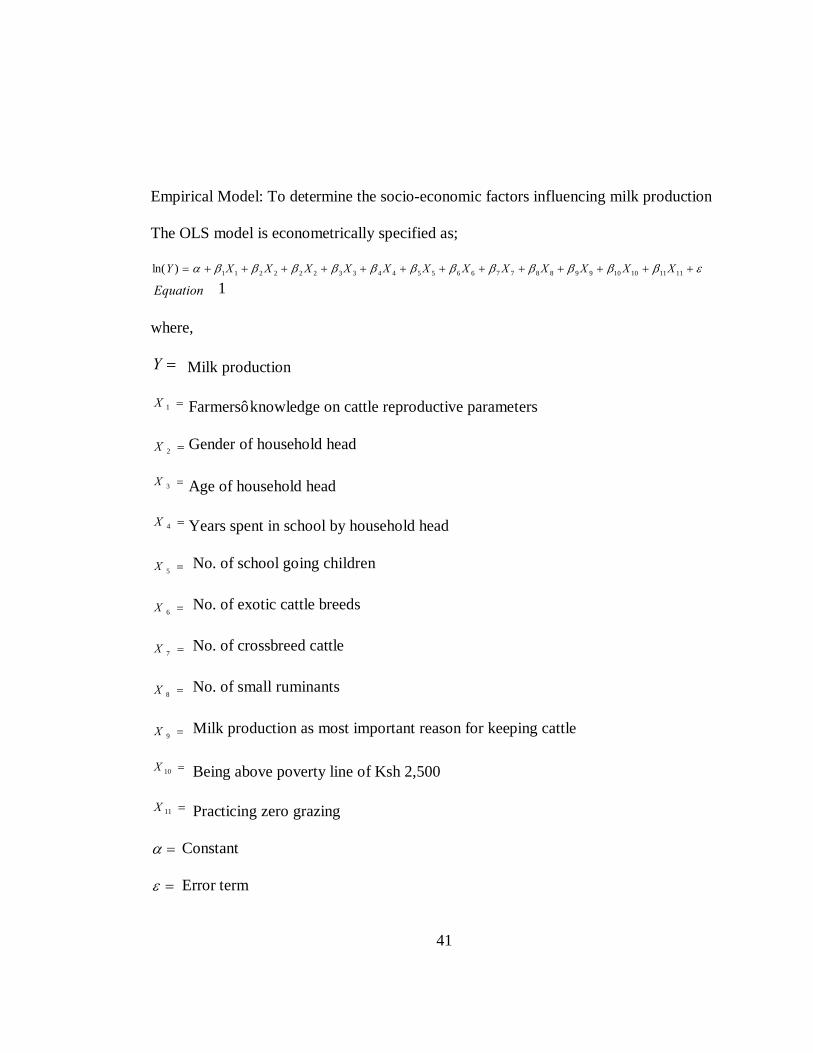
Empirical Model: To determine the socio-economic factors influencing milk production
The OLS model is econometrically specified as;
εββββββββββββα +++++++++++++= 1111101099887766554433222211)ln( XXXXXXXXXXXXY
Equation 1
where,
=Y Milk production
=1X Farmers’ knowledge on cattle reproductive parameters
=2X Gender of household head
=3X Age of household head
=4X Years spent in school by household head
=5X No. of school going children
=6X No. of exotic cattle breeds
=7X No. of crossbreed cattle
=8X No. of small ruminants
=9X Milk production as most important reason for keeping cattle
=10X Being above poverty line of Ksh 2,500
=11X Practicing zero grazing
=α Constant
=ε Error term

42
nββ ....1 = Coefficients
The OLS was used to obtain the coefficient estimates of nββ .........1\
Table 3.3: Explanatory variables in the model on factors influencing milk
production and their expected contribution
Variable Definition Expected sign
Farmers knowledge of the cattle reproductive parameters
Knowledge of farmers on the length of gestation, calving to conception interval, calving to first heat, age at first heat, signs of pregnancy in cows and heat signs
+
Gender of household head 1 if male, zero otherwise - Age of household head Age in years + Years spent in school by household head
Formal years the household head has spent in school
+
No. of school going children Number of children going to school ± No. of exotic cattle Number of exotic cattle breed + Practicing zero grazing 1 if farmers practices zero grazing and 0
otherwise +
No. of crossbreed cattle Number of crossbreed cattle owned by the household
+
No. of small ruminants Number of sheep and goats owned by the household
_
Poverty line of Ksh.2,500 1 = Being above poverty line of Ksh 2,500 and 0 otherwise
+
3.5.1 Goodness-of-fit measure
Model fit statistic summarizes how well a set of explanatory variables explains a response
variable. Among the goodness of fit measures is the R2 statistic also known as the
coefficient of multiple determinations. It is a common statistics used to determine OLS

43
model fitness. It indicates the percentage of variation in the response variable that is
explained by the model. The value of R2 is always between zero and one. When
interpreting R2, its value is multiplied by 100 to change it into a percentage. If the data
points all lie on the same line, OLS provides a perfect fit to the data. In this case, R2 equals
one. A value of R2 that is nearly equal to zero indicates a poor fit of the OLS line. That
means that very little of the variation in the Y is captured by the variation in the predicted Y
(Wooldridge, 2003). This was obtained for the two OLS models on factors influencing
knowledge and milk production.
3.5.2 Identification of powerful instrumental variables
Instrumental variables are variables that are explicitly excluded from some equations and
are included in others and therefore correlated with some outcomes only through their
effect on other variables (Angrist et al., 1996). In this study, partial correlations were used
to identify the instrumental variables those that would influence farmers’ knowledge of the
cattle reproductive parameters but through zero grazing.
3.5.3 Hausman test
In any production function, all inputs are expected to be exogenous in simple terms
explanatory variables. Exogeneity is critical in ensuring that estimates are not biased
(Carpentier and Weaver, 1997). However, there are scenarios where one or more
inputs/variables are endogenous (dependent variable) and not exogenous. In this case,
44
participation in zero grazing as one of the variables influencing farmers’ knowledge was
suspected to be endogenous. In technology adoption, the problem of endogeneity emerges
because technology adoption is either voluntary or some technologies are targeted to a
given group of farmers (Hausman, 1978). In circumstances where technology adoption is
voluntary, it is the more productive farmers that are more likely to adopt the technology.
This self-selection into technology adoption may be source of endogeneity. Failure to
account for this will overstate the true impact of the technology. On the other hand, in
circumstances where technology is targeted to a given group of farmers, it is far more likely
that less productive farmers will adopt the technology. Failure to account for this will
understate the true impact of the technology. These two scenarios make it difficult to
estimate the true impact of the technology adoption on any variable (Hausman, 1983) for
instance income and knowledge among others.
When choosing the estimation method, where endogeneity is a problem, consistent
estimates can be obtained by suitably instrumenting the relevant variable using the 2SLS
estimator. On the other hand, where endogeneity is not a significant problem, the least
squares estimator is more efficient than instrumental variables (Wooldridge, 2003).
However, both OLS and 2SLS are consistent if all variables are exogenous (Wooldridge,
2003). In this study, to determine factors that influence farmers’ knowledge of the cattle
reproductive parameters the problem of endogeneity was suspected to be present; hence,
the two models ( 2SLS and OLS) had to be run and Hausman test had to be performed in
order to choose the appropriate estimation method. When the Hausman test (Hausman,

45
1978) probability chi-square value turns out insignificant then that indicates that OLS
model estimation is appropriate and when it turns out significant that implies that 2SLS
model estimation is appropriate.
3.5.4 Testing for heteroskedasticity
Heteroskedasticity exists when the variances of all variables are not the same, leading to
consistent but inefficient parameter estimates (Breusch and Pagan, 1979). There are many
tests for heteroskedasticity. These make different assumptions about the form of
heteroskedasticity, tests such the Breusch-Pagan test can be used to detect
heteroskedasticity. The Breusch-Pagan / Cook-Weisberg test is used to test for the linear
form of heteroskedasticity. In this study the Breusch-Pagan / Cook-Weisberg test was used.
It tests the null hypothesis that the error variances are all equal versus the alternative that
the error variances are a multiplicative function of one or more variables. From the results,
a large chi-square indicates that heteroskedasticity is present while a small chi-square value
indicates heteroskedasticity is probably not a problem (Breusch and Pagan, 1979).
Alternatively, if the test results in a small enough p-value, some corrective measure should
be taken (Wooldridge, 2003). However, if heteroskedasticity is found present OLS
regression gives still appropriate coefficient estimates, but test statistics have to be adjusted
to the heteroskedasticity-robust standard error or the heteroskedasticity-robust t statistic
(Wooldridge, 2003). The Breusch-Pagan / Cook-Weisberg test was performed in both OLS
models; determining factors influencing knowledge and milk production.
46
CHAPTER 4
RESULTS
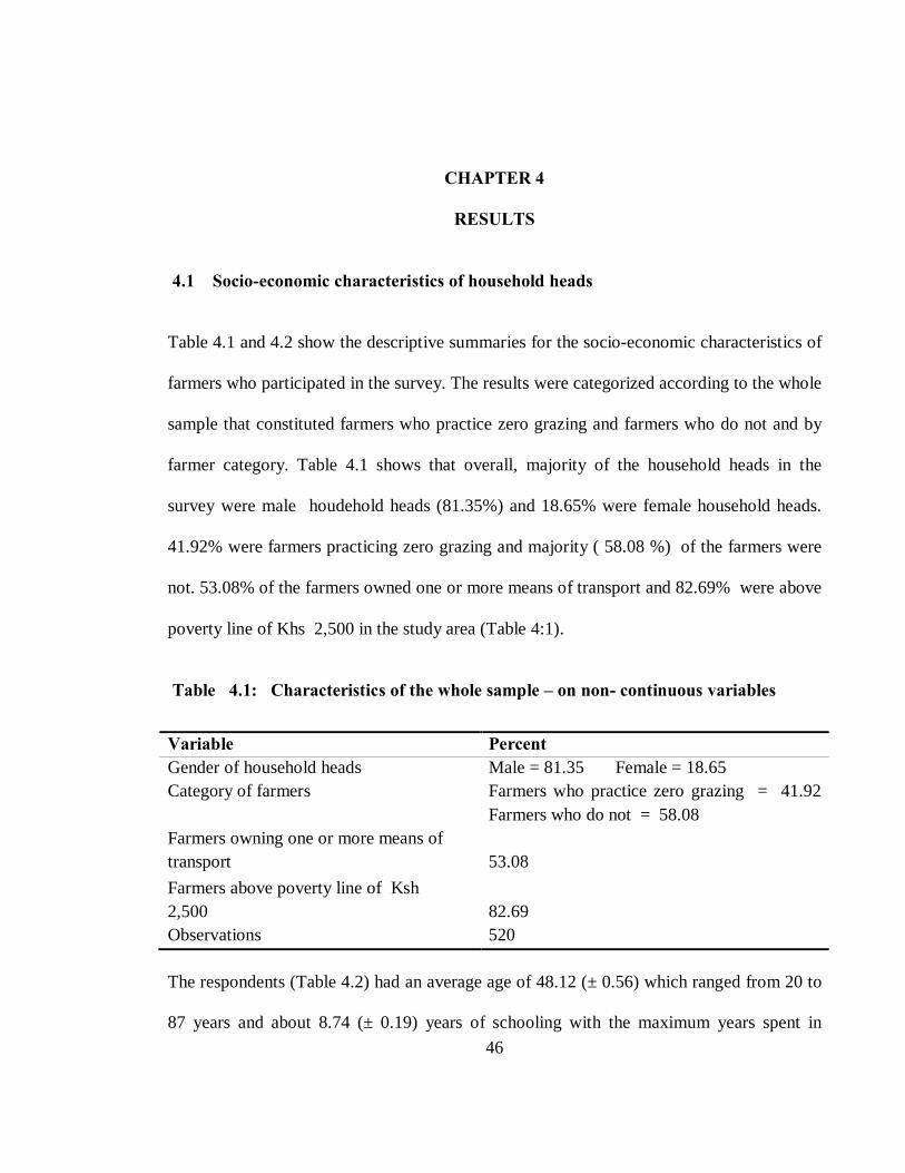
4.1 Socio-economic characteristics of household heads
Table 4.1 and 4.2 show the descriptive summaries for the socio-economic characteristics of
farmers who participated in the survey. The results were categorized according to the whole
sample that constituted farmers who practice zero grazing and farmers who do not and by
farmer category. Table 4.1 shows that overall, majority of the household heads in the
survey were male houdehold heads (81.35%) and 18.65% were female household heads.
41.92% were farmers practicing zero grazing and majority ( 58.08 %) of the farmers were
not. 53.08% of the farmers owned one or more means of transport and 82.69% were above
poverty line of Khs 2,500 in the study area (Table 4:1).
Table 4.1: Characteristics of the whole sample – on non- continuous variables
Variable Percent Gender of household heads Male = 81.35 Female = 18.65 Category of farmers Farmers who practice zero grazing = 41.92
Farmers who do not = 58.08 Farmers owning one or more means of transport
53.08
Farmers above poverty line of Ksh 2,500
82.69
Observations 520
The respondents (Table 4.2) had an average age of 48.12 (± 0.56) which ranged from 20 to
87 years and about 8.74 (± 0.19) years of schooling with the maximum years spent in

47
school being 19. The average number of school going children was 2.53 (± 0.10) per
household (Table 4.1) with a maximum of 16. The average herd size was 3.28 (± 0.10) and
21 was the maximum. The mean number of exotic cattle was 1.09 (± 0.08), maximum was
13. The mean dependency ratio was 1.16 (± 0.06) and 12 being the maximum. For
crossbreeds, mean number was 1.23 (± 1.68) with a maximum of 11 (Table 4.1).The mean
number of small ruminants was 0.86 (± 0.07) with maximum of 13. The overall average
milk produced per lactation period per cow was 940.55 (± 48.86) litres with 6,480 litres
being the maximum.
Table 4.2: Characteristics of the whole sample – on continuous variables
Variable Mean Minimum Maximum Age of household head 48.12 ± 0.56 20 87 Years spent in school by household head 8.74 ± 0.19 19 No. of school going children 2.53 ± 0.10 16 Herdsize 3.28 ± 0.10 21 No. of exotic cattle 1.09 ± 0.08 13 Dependency ratio 1.16 ± 0.06 12 No. of cross breed cattle 1.23 ± 1.68 11 No. of small ruminants 0.86 ± 0.07 13 Milk production( litres per lactation period per cow)
940.55 (± 48.86)
6,480
Observations 520
4.2 Socio-economic characteristics by category of farmers
Using the two sample t-test that tests for the statistical differences between two means the
results ( Table 4.3) show that farmers who practice zero grazing had (49.49 ± 0.79) years
48
on average whilst those that do not had (47.12 ± 0.77). Testing for the statistical differences
in age of the farmers showed that there were significant differences between the two groups
(P = 0.04). Farmers that practice zero grazing had spent (9.96 ± 0.29) years in school on
average and those who do not had spent (7.86 ± 0. 23). The differences in attaining
education between the two groups were significant (P = 0.00) (Table 4.3).
The farmers who practice zero grazing had on average a herd size of 3.65 ± 0.15 while
those who do not had (3.00 ± 0 .12). The differences in herd size between the two groups
were significant (P = 0.00). Farmers who practice zero grazing had (2.28 ± 0.14) exotic
cattle on average whilst those who do not had (0.24 ± 0.05). The difference in the average
number of exotic cattle owned was significant (P = 0.00). Farmers who practice zero
grazing had on average (0.82 ± 0.11) number of cross breed cattle while those that do not
had (1.53 ± 0.09). The differences was significant (P = 0.00). Farmers who practice zero
grazing had a mean dependency ratio of (1.31 ± 0.08) on average while that of farmers who
do not had (0.96 ± 0.090). The results showed that significant differences (P = 0.00) existed
between the two groups. The farmers who practice zero grazing had (1.28 ± 0.03) number
of school-going children and those who do not had (3.44 ± 0.15). The differences in
number of school going children were significant (P = 0.00).
There were no significant differences observed between the two groups regarding the
number of small ruminants owned. The farmers who practice zero grazing produced

49
1405.56 litres of milk per lactation period per cow than their counterparts 604.87 such a
difference was significant (P = 0.00) (Table 4.3).
Table 4.3: Means of variables, by category of farmers
Variable Farmers who practice zero grazing Farmers’ who do not P- value
Age of household head 49.49 ± 0.79 47.12 ± 0.77 0.04 Years spent in school by household head
9.96 ± 0.29
7.86 ± 0.23
0.00
No. of school going children
1.28 ± 0.03
3.44 ± 0.15
0.00
Herdsize 3.65 ± 0.15 3.00 ± 0 .12 0.00 No. of exotic cattle 2.28 ± 0.14 0.24 ± 0.05 0.00 Dependency ratio 0.96 ± 0.09 1.31 ± 0.08 0.00 No. of crossbreed cattle 0.82 ± 0.11 1.53 ± 0.09 0.00
No. of small ruminants 0.94 ( ± 0.13) 0.80 ( ± 0.08) 0.13
Milk production (ltrs, per lactation/cow)
1405.56 ± 88.45
604.87 ± 46.09
0.00
Observations 218 302
Note: Data are computed using a two- sided t test
Table 4.4 shows that with regard to gender, out of the farmers practicing zero grazing
81.46% were male household heads and out of those not practicing zero grazing, the males
constituted 81.19%. There were no significant differences noticed between the two groups
(P = 0.94) regarding the proportion of their male composition. Out of the farmers practicing
zero grazing, those who were above the poverty line of Ksh 2,500 were 91.74% and out of
the farmers not practicing zero grazing, those that were above the poverty line of Ksh.

50
2,500 were 76.16%. The percentage differences of farmers above the poverty line of Ksh
2,500 of the two groups were significant (P = 0.00). Significant differences (P = 0.00) were
observed in the ownership of one or more means of transport between the two groups.
64.22% of the farmers who practice zero grazing had at least one or more means of
transport while 45.03% of those who do not practice zero grazing owned at least one or
more means of transport (Table 4.4).
Table 4.4: Percentage values of variable by category of farmers
Variables Farmers who practice zero grazing Farmers’ who do not P- value
Male household heads
81.46%
81.19%
0.94
Being above poverty line of Ksh 2,500
91.74%
76.16%
0.00
Owning one or more means of transport
64.22%
45.03%
0.00
Observations 218 302
Note: Data are computed using a two- sample proportions z- test
4.3 Logistic regression on factors influencing adoption of zero grazing
To determine factors influencing adoption of zero grazing (Table 4.5) presents the logistic
regression odds ratio, standard errors, z values, p - values and confidence intervals of
factors influencing adoption of zero grazing. With the exception of male household heads
and number of crossbreeds, the rest of the explanatory factors had the expected signs. In

51
model selection, several possible models were fitted by dropping and adding variables
expected to influence participation. The model that gave good results according to R2
(Appendix 1.1), goodness of fit (Appendix 1.2), multicollinearity test (Appendix 1.3) and
correct predictions (Appendix 1.4) was retained and used for interpretation of results. The
R2 explained 59% of the total variation, the goodness of fit test (Hosmer-Lemeshow
goodness- of- fit test) obtained a chi-square value of 13.34 with a high probability value
0.10, the average variance inflation factors (VIF), was 1.27 and the proportion of the total
number of predictions correctly estimated was about 87.12%.
Table 4.5: Logistic regression on factors influencing adoption of zero grazing
Variable Odds ratio
Standard error
Z P- value [95% conf. Interval]
Male household heads 0.7 0.3 -1.0 0.32 0. 304 - 1.478
Age of household heads 1.0 0.0 2.2 0.03 1.003 - 1.049
Years spent in school by household head 1.1 0.5 3.2 0.00 1.051 - 1.234
No. of school going children 0.3 0.0 -8.4 0.00 0.221 - 0.391
Herd size 0.9 0.1 -1.3 0.19 0.773 - 1.052
No. of exotic cattle breeds 5.0 0.9 8.6 0.00 3.465 - 7.196
Being above poverty line of Ksh 2,500 2.9 1.3 2.3 0.02 1.162 - 7.139
Dependency ratio 1.4 0.2 2.2 0.03 1.042 - 1.939
Owning one or more means of transport 1.4 0.3 1.3 0.21 0.850 - 2.131
No. of crossbreed 1.2 0.1 1.9 0.05 0.997 - 1.492
No. of small ruminants 1.0 0.1 -0.3 0.74 0.797 - 1.174

52
The results (Table 4.5) show that with the exception of male household heads, the number
of school going children, herd size, and the number of small ruminants, all other variables
in the model had positive influence on farmers’ adoption of zero grazing. The decision by
household heads to adopt zero grazing was significantly influenced by the following socio-
economic variables (P < 0.05). The age of household heads, number of years spent in
school by household heads, number of school going children, number of exotic cattle, being
above poverty line of Ksh 2,500, dependency ratio, and number of crossbreed cattle. The
odds ratios for age of household head, years spent in school by household head, number of
exotic cattle breeds, being above poverty line of Ksh 2,500, dependency ratio and number
of crossbreed cattle were 1.0, 1.1, 5.0, 2.9, 1.4 and 1.2 respectively (Table 4.5). The
variables male household heads, herd size, owning one or more means of transport and
number of small ruminants were not significant in influencing zero grazing adoption.
4.4 Farmers knowledge on the cattle reproductive parameters in western Kenya -
whole sample
To assess farmers’ knowledge on the cattle reproductive parameters (Table 4.6 ) shows
that on average, farmers’ knowledge ranged from 4.7% to 18.3% on the parameters. On
average, farmers obtained 17.1% on their knowledge of gestation length with a maximum
of 42.9%.The mean knowledge on calving to conception interval was 14.1%, with a
maximum of 71.4%. The knowledge on calving to first heat was 4.7% on average with
maximum of 40%. On average farmers’ obtained 18% with a maximum of 60% on age at
first heat, (Table 4.6).Their knowledge on pregnancy signs was on average 13.0% with a

53
maximum of 37.5%. The findings showed that when the knowledge of farmers on all the
parameters was combined, 9.9 % on average was obtained with a maximum of 22.7%
(Table 4.6).
Table 4.6: Overall knowledge of livestock farmers on cattle reproductive
parameters
Reproductive parameters Overall mean Maximum (%) Length of gestation period 17.1 ± 0.4 42.9 Calving to conception interval 14.1 ± 0 .5 71.4 Calving to first heat 4.7 ± 0.4 40 Age at first heat 18.3 ± 0.7 60 Pregnancy signs 13.0 ± 0.3 37.5 Heat signs 6.5 ± 0.1 14.7 All parameters combined 9.9 ± 0.2 22.7 Observations 520
4.5 Farmers’ knowledge on the cattle reproductive parameters by category of farmers
To establish the knowledge difference between the two groups (Table 4.7) shows that
farmers who practice zero grazing had more knowledge on the parameters than farmers
who do not practice zero grazing on a snapshot. Farmers who practice zero grazing
obtained 21.45% over (7) on gestation length, 19.55% over (7) on calving to conception
interval, 5.32 over (5) on calving to first heat, 18.44 over (5) on age at first heat,13.65 over
(8) on pregnancy signs and 7.35 over (34) on heat signs. While those who do not practice
zero grazing obtained 14.02% over (7) on gestation length, 10.23% over (7) on calving to
conception interval, 4.24% over (5) on calving to first heat, 18.15% over (5) on age at
first heat, 12.54% over (8) on pregnancy signs and 5.88% over (34) on heat signs. These

54
findings indicated that overall knowledge of farmers’ who practice zero grazing on the
parameters was 11.59% over (66) which was higher than that of the farmers who do not
practice zero grazing (8.8%) (Table 4.7).
Table 4.7: Farmers knowledge on cattle reproductive parameters in western
Kenya by category of farmers
Reproductive parameters
Farmers who practice zero grazing Farmers who do not P- Value
Length of gestation period
21.45 ± 0.40
14.02 ± 0.68
0.00
Calving to conception interval
19.55 ± 0.86
10.23 ± 0.58
0.00
Duration from calving to first heat
5.32 ± 0.68
4.24 ± 0.50
0.19
Age at first heat 18.44 ± 1.06 18.15 ± 1.02 0.84 Pregnancy signs 13.65 ± 0.45 12.54 ± 0.35 0.05 Heat signs 7.35 ± 0.19 5.88 ± 0.16 0.00 Total on the farmers’ knowledge of cattle reproductive parameters
11.59 ± 0.24
8.82 ± 0.18
0.00
Observations 218 302
Note: Data were computed using a two- sided t test.
Using the two-sample t test significant differences between the groups were noticed
regarding their knowledge on length of gestation period (P = 0.00), calving to conception
interval (P = 0.00), heat signs and pregnancy signs (P = 0.00). Regarding their knowledge
on calving to first heat (P = 0.19) and age at first heat (P = 0.84) there were no significant

55
differences between both groups. On average the differences range between 0.29 in the
category of knowledge on age at first heat, up to 9.32 knowledge score on calving to
conception interval.
4.6 Factors influencing farmers’ knowledge of cattle reproductive parameters in
western Kenya
The ordinary least squares regression was applied to explore the relationship between
farmers’ knowledge on the cattle reproductive parameters and the socio-economic
variables. The analysis was undertaken on 510 respondents after removal of outliers.
Appendix (3.0), the subsequent sections, and Table (4.8) show results on factors
influencing farmers’ knowledge of the cattle reproductive parameters. The correlation
matrix (Appendix 3.1) illustrates that some variables are statistically correlated but none
had a correlation coefficient of greater than 0.9. The partial correlation results for the
number of exotic cattle owned, poverty line and dependency ratio were (r = 0.14, P = 0.00),
(r = 0.55, p = 0.00) and (r = - 0.09, p = 0.04) respectively (Appendix 3.2). Hausman test
turned out to have a probability chi-square value of 0.6019 (Appendix 3.3). The R2 obtained
was 0.21 (Appendix 3.4).The variance Inflation Factors (VIFs) (Appendix 3.5) attained a
maximum value of 1.38. The Breusch-Pagan /Cook-Weisberg test gave a p-value of Prob >
chi2 = 0.85 (Appendix 3.6).
Table 4.8 depicts that practicing zero grazing and number of exotic cattle breed influenced
farmers’ knowledge of reproductive parameters at (P = 0.00) and ( P = 0.00) respectively.
The anticipated positive impact of practicing zero grazing on farmers’ knowledge of the

56
cattle reproductive parameters becomes evident. Holding all other factors constant, farmers’
knowledge of the reproductive parameters is more likely to increase by 1.6% if adoption of
zero grazing increases by 1%. Number of exotic cattle owned by farmers positively and
significantly influenced farmers’ knowledge of the cattle reproductive parameters.
Increasing the number of exotic cattle by one exotic cow was more likely to increase
farmers’ knowledge of the reproductive parameters by 0.02% (Table 4.8).
Table 4.8: Ordinary least squares regression on factors influencing farmers’
knowledge of cattle reproductive parameters
Variables Coefficients Std Errors ‘t’ values P-value Age of household head 0.19 0.01 -1.70 0.09 Year spent in school by household head -0.00 0.03 -0.09 0.93 No. of school going children 0.03 0.07 -0.37 0.71 Milk production as the most important reason for keeping cattle
0.62
0.34
1.81
0.07
Male household heads 0.23 0.36 0.66 0.51 Herdsize 0.14 0.07 1.88 0.06 Owning one or more means of transport 0.34 0.22 1.53 0.13 No. of crossbreed cattle 0.14 0.09 1.48 0.14 No. of small ruminants 0.00 0.08 -0.11 0.91 Practicing zero-grazing 1.6 0.38 4.23 0.00 Dependency ratio 0.05 0.01 0.51 0.61 Being above poverty line of Ksh 2,500 0.24 0.05 0.66 0.51 No. of exotic cattle 0.02 0.37 2.93 0.00
1 Dependent variables: Farmers’ knowledge of cattle reproductive parameters

57
4.7 Factors influencing milk production
The results of the ordinary least squares regression model were used to determine the
factors that influenced milk production (Table 4.9).The response variable was the
transformed milk production variable. The exogenous variables were; age of household
head, years spent in school by household head, number of school going children, milk
production as the most important reason for keeping cattle and gender of household head.
Others included herd size, means of transport, number of crossbreed cattle, number of small
ruminants, practicing zero grazing, dependency ratio, being above poverty line of Ksh
2,500 and number of exotic cattle. The correction matrix (Appendix 4.1) revealed the
correlation coefficient between any pair of explanatory variables to be less than 0.9 in
absolute value. The obtained R2 was 0.22 (Appendix 4.2). The variance inflation factor
(VIF) was also calculated and was found to be 1.29 (Appendix 4.3). The Breusch-
Pagan/Cook-Weisberg test for heteroskedasticity had a high chi-square value of 0.11
(Appendix 4.4).
The results (Table 4.9) show that male household heads negatively and insignificantly
influenced the adoption of zero grazing. Explanatory variables such as age of household
head, year spent in school by household head, number of school going children, number of
small ruminants positively but insignificantly influenced the adoption of zero grazing. Only
six explanatory variables namely farmers’ knowledge of cattle reproductive parameters,
number of exotic cattle, number of cross breed cattle, milk production as most important

58
reason for keeping cattle, being above poverty line of Khs 2,500 and practicing zero
grazing influenced milk production.
Table 4.9 shows farmers’ knowledge of cattle reproductive parameters positively
influenced milk production. The sign is in accordance to the expectations that farmers’
knowledge positively influences milk production. In fact, a 10% increase in farmers’
knowledge will likely increase the milk production per lactation period of cow by 1.59%
per year, holding other factors constant. As anticipated, number of exotic cattle owned by
farmers positively and significantly influenced milk production. Infact, increasing the
number of exotic cattle owned by farmers’ by 10% will likely increase the milk production
per lactation of a cow by 2.8% ceteris paribus. In addition, number of crossbreed cattle
owned by farmers positively and significantly influenced at 5% milk production. A 10%
increase in the number of crossbreed cattle owned will likely increase the milk production
per lactation period of cow by 2.7% per year. This is in line with the expectations. In
accordance to expectations, milk production as the most important reason for keeping cattle
positively and significantly, increases milk production at 5%. Increasing the milk
production, as the most important reason for keeping cattle, is more likely to increases milk
production (Table 4.9).
The sign as expected being above poverty line Ksh of 2,500 positively and significantly at
5% increases milk production. Being above the poverty line of Ksh of 2,500 was more
likely to increase milk production. In line with the expectations, practicing zero grazing

59
positively and significantly influenced milk production. Increasing participation in zero
grazing was more likely to increase milk production.(Table 4.9).
Table 4.9: Ordinary least squares regression on factors influencing milk production
Predictor variables Coefficients Std Errors P-
value ‘t’ values
Knowledge on cattle reproductive parameters
1.6 0.3 0.000 4.7
Male household head -0.3 0.4 0.457 -0.8 Age of household head 0.0 0.0 0.732 0.3 Year spent school by household head 0.0 0.0 0.250 1.2 No. of school going children 0.1 0.1 0.273 1.1 No. of exotic cattle 0.3 0.1 0.003 3.0
No. of crossbreed cattle 0.3 0.1 0.001 3.2
No. of small ruminants 0.1 0.1 0.473 0.7 Milk production as the most important reason for keeping cattle
1.3
0.4
0.000
3.7
Being above poverty line of Ksh 2,500 1.0 0.4 0.009 2.6
Practicing zero grazing 0.8 0.4 0.015 2.2
2 Dependent variable: Milk production

60
CHAPTER 5
DISCUSSION
5.1 Socio-economic characteristics of the household heads
5.1.1 Characteristics of the whole sample – on non- continuous variables
The target population was the household heads thus the findings revealed that male
household heads dominated the survey. This means that livestock production in the study
area is an activity mostly preferred by the males. They are the household heads, they own
the resources, and at the same time, they are decision makers hence decide upon which
economic activity to take on. The studies carried out in Tanzania and North western
Ethiopian highlands found that male household heads constituted the highest percentages
which were not very different from (81.35%) as obtained in this study (Swai et al., 2005
and Ayenew et al., 2011). The proportion of farmers not practicing zero grazing in the
survey was higher than that of farmers who practice zero grazing, meaning that majority of
the small scale farmers residing in the study area are yet to appreciate zero grazing.
Livestock production is an income generating activity; the incomes generated enable
livestock farmers to acquire at least one or more means of transport. The high percentage of
farmers above the poverty line of 2,500 is explained by the fact that, farmers who
participated in the survey were livestock keepers, so they own the cattle, sell milk, and
cattle to generate income hence obtain higher household incomes.

61
5.1.2 Characteristics of the whole sample – on continuous variables
The mean age of the respondents that participated in this survey is not very different from
that obtained by Staal et al. (2001) in a similar study carried out in Kenya. This implies that
livestock production in this country is highly appreciated by people who are around the age
of 48. The average years spent by the household heads in school were relatively high; this
means that education plays an important role in livestock production.
The results of the survey revealed that household heads on average had three school going
children. This is an indication that the livestock farmers in the study area value education
that is why atleast on average each household managed to have 3 children in school. The
average herd size is similar to that obtained by Bebe et al. (2003) in a similar study carried
out in Kenya Highlands. In both study areas, small-scale farmers keep three cattle on
average. This could be explained by the high human population growth rate, which has led
to intergeneration sub division and fragmentation of farms in Kenya (C.B.S., 2001). As
human population growth increases, the number of land holdings increase but these get
smaller with smaller herds (Bebe et al., 2003). It is not surprising that at least each
household owned on average one exotic cow. Exotic cattle are among the main breeds used
for dairy production in Kenya (Omore et al., 1998). From these findings, the obtained
dependency ratio was low implying that the dependency burden is lighter. Household heads
in the study area owned 1.23 crossbreeds. Cross breeding of indigenous breeds with exotic
breeds is a strategy being promoted in developing countries to improve milk production of
indigenous breeds (Darfour-Oduro et al., 2010).
62
The study revealed that livestock farmers in the study area keep other livestock (small
ruminants though in small numbers compared to cattle). This is in line with Jaetzold et al.
(2005) who observed that farmers in Bungoma County keep goat, sheep, poultry although
to them cattle are the major form of livestock. The multiple benefits derived from keeping
cattle explain why the livestock farmers in the study area prefer keeping more cattle
compared to small ruminants. The average milk figures reported (940.55 litres per lactation
period) indicated that there is milk produced within the study area and this could be
attributed to exotic and indigenous cattle breeds kept within the study area (Census, 2009).
5.2 Socio-economic characteristics by category of farmers
5.2.1 Means of variables, by category of farmers
Farmers who practice zero grazing were significantly older than the farmers who do not.
Being older means that they have more command over resources that explain their
participation in zero grazing. Farmers who practice zero grazing had significantly spent
more years in school. With more years spent in school, they are better positioned to
recognize the importance of zero grazing as compared to those with lesser years of
schooling. Farmers who practice zero grazing in the study area had a significantly higher
mean herd size than the farmers who do not. High cattle herd sizes in small-scale farms in
Eastern Cape Province (Mapekula et al., 2009) were attributed to resource ownership and
affordability of feed. Farmers who practice zero grazing had significantly more number of
exotic cattle than the farmers who do not practice zero grazing. It is uncommon to find

63
exotic breeds of cattle under a non zero grazing system. Farmers who do not practice had a
significantly higher dependency ratio than farmers who do practice zero grazing. This could
be attributed to the fact that households with a higher dependency ratio (non-labour force to
the labour force) have more dependents to cater for, hence lesser resources to invest in
zero grazing.
Farmers who do not practice zero grazing afforded significantly more crossbreed cattle that
require minimal investment. Supported by this is Lanyasunya et al. (2006) who argues that
crossbreed cattle dominate the free-grazing herds rather than zero grazing dairy systems.
No significant differences were noted between farmers who had practiced zero grazing and
n farmers who do not. The farmers who practice zero grazing realized more than twice the
amount of milk in litres than the farmers who do not practice zero grazing. Similar to this,
in a study by Karanja (2003) the yields realized in smallholder open grazing farms were
lowest as compared to milk yields in the small scale zero grazing. The milk yield under the
smallholder open grazing farms averaged to 1,510 litres per cow per year. This yield was
28.8% lower than the average yields in small scale zero grazing. The differences in
productivity were attributed to access to production services and level of management.
5.2.2 Percentage values of variable by category of farmers
There were no significant differences witnessed between the male composition of farmers
who practice zero grazing and those that do not. The higher proportion of farmers who
practice zero grazing noticed being above the poverty line of Ksh 2,500 explains the fact

64
that zero grazing dairy system requires more capital than the open grazing system.
Adoption of zero grazing requires relatively more resources. Leegwater et al. (1991) in a
study in the Kenyan coast, found out that the zero- grazing system, was adopted mainly by
the rich farmers who could afford the initial investment requirements which entailed the
purchase of a grade cow and the building of a stall, which poor farmers’ could not afford.
Nicholson et al. (1998), argues that the principal reasons farmers are not adopting dairy
cattle is because of lack of money to purchase the animal and lack of credit. A significantly
higher percentage of farmers who practice zero grazing owned at least one or more means
of transport than the farmers who do not. This implies that the farmers who practice zero
grazing have more resources. In agreement to this is (Jera and Ajay, 2008) points out that
farmers with more resources are more likely to invest in new technologies.
5.3 Determination of socio-economic factors influencing adoption of zero grazing
using logistic regression
The obtained Hosmer-Lemeshow goodness- of- fit test implied that the chosen model fits
well the data and that the explanatory variables adequately explain the probability of
adoption of zero grazing since the obtained Chi Square is high. The VIF, which was less
than 10, which implied that multicollinearity, was not a problem (Meyers, 1990).
In this study, it was hypothesized that older people are more likely to adopt zero grazing
and the results of the study conforms to the expectations. The observed positive relationship
between age of household head and adoption of zero grazing implies that older farmers are
65
more likely to adopt zero grazing. The obtained odds ratio of age of household head implies
that older people are 1.03 times more likely to influence adoption of zero grazing. This is
probably because age is related to experience and therefore older farmers are likely to be
more experienced and able to discern the importance of improved technology more as
compared to the less experienced young farmers (Murage and IIatsia, 2011). Our results
agree with those of Kafle and Shah (2012) and Shields et al. (2012) who observed a
positive and significant relationship between age and technology adoption. Similarly Tambi
et al. (1999) reported a positive and significant relationship between demand for improved
technology and producers within the age group 25 to 50 years compared to those who were
less than 25 years in Kenya
The positive relationship between years of schooling and adoption of zero grazing was
expected. Years of schooling had a positive and significant influence on adoption of zero
grazing. In this study, it implies that household heads that have more years of schooling are
more likely to participate in zero grazing than those with lesser years. The odds ratio
implies that farmers who have more years of schooling are 1.14 times more likely to adopt
zero grazing than their counterparts are. Earlier studies Nichinda and Mendi (2008);
Karamjit et al. (2009); Musaba (2010); Murage and IIatsia (2011) and Fita et al. (2012)
found out that years spent in school by household heads had a positive and significant
influence on the adoption of technologies. These findings are consistent with the findings of
this study.

66
The more educated a household head is, the more he/she is likely to acquire, understand,
obtain, disseminate new technologies within a shorter time and more efficient when
allocating resources compared to a household head with fewer years of education (Kafle
and Shah 2012; Ebojei et al. (2012). Similarly, education makes people realize the
importance and benefits of adopting new technologies (Musaba, 2010). Along the same
line, Foster and Rosenzweig (1996) argued that farmers who are more educated are more
able to manage new technologies or became aware of productive innovations at earlier
stages of growth than their less- educated counterparts.
It was hypothesized that a positive relationship would exist between the number of exotic
cattle breeds owned by the farmers and adoption of zero grazing. In the present study,
number of exotic cattle owned by farmers positively and significantly influenced adoption
of zero grazing. The odds ratio for number of exotic breed cattle implied that number of
exotic cattle breeds was 5.0 times more likely to influence the adoption of zero grazing.
The positive relationship between number of exotic cattle and adoption of zero grazing is in
agreement with Kaaya et al. (2005) who observed that farmers who keep exotic cattle are
more likely to use improved technology. The results are also agreed with the
recommendation of Murage and IIatsia (2011) who observed that farmers who kept
purebred dairy cattle would more likely opt for improved technology. In this study
household heads with more numbers of exotic cattle are more likely to participate in zero
grazing. Exotic breeds are confined under zero grazing units where feed and water are
brought to the animals. Further, zero grazing reduces exposure of the valuable cows to

67
many vector diseases (Muraguri, 2000) and ensures strict isolation of the exotic cattle from
the indigenous cattle (De-wit, 1990). It also safe guards cows from tick borne diseases and
other health hazards (Mango, 2002).
The positive relationship between dependency ratio and adoption of zero grazing supports
the hypothesis that higher dependency ratio is more likely to influence the adoption of zero
grazing. The odds ratio for dependency ratio implies that dependency ratio is 1.4 times
more likely to influence the adoption of zero grazing. The positive relationship between
dependency ratio and adoption of zero grazing disagrees with Owu (1995) who argues that
dependency ratio is negatively related to adoption decisions, since a high dependency ratio
adds pressure on household consumption. This is in agreement with the findings of Ojaiko
et al. (2007) and Ojaiko (2011) who argue that high dependency ratio increases the
obligatory burden on the household head. The household head who is always worried with
how to meet the immediate household needs, will be less willing to risk the fewer resources
on new technologies.
In this study, it was hypothesized that the number of cross breed cattle owned negatively
influenced adoption of zero grazing. On contrast, the findings of this study revealed that,
the number of crossbreed cattle positively influences adoption of zero grazing technology.
The odds ratio for number of crossbreed implies that number of crossbreed cattle is 1.22
times more likely to influence adoption of zero grazing. This is consistent with Kaaya et al.
(2005) who argues that a farmer keeping crossbred cattle is more likely to use AI

68
technology. The results of this study reveal that a farmer with more crossbreed cattle was
more likely to participate in zero grazing. The way crossbreed cattle are managed is not
different from exotic breeds of cattle, so zero grazing is indispensable.
In this study, it was hypothesized that being above the poverty line of Ksh 2,500 was more
likely to influence the adoption of zero grazing. Indeed a positive relationship was observed
between being above poverty line of Ksh 2,500 and adoption of zero grazing. The odds
ratio for being above poverty line of Ksh 2,500 implies that being above the poverty line of
Ksh 2,500 was 2.9 times more likely to influence the adoption of zero grazing. The results
of the study are in agreement with the findings of Irungu et al. (1998); Waithaka et al.
(2007) and Shields et al. (2012) who observed a positive relationship between household
income and adoption of a new technology. In this study, farmers’ above the poverty line of
Ksh 2,500 were more likely to adopt zero grazing. Being above the poverty line of Ksh
2,500 implies that a household is able to meet its basic needs and still have surplus income
to invest in zero grazing.
5.4 Farmers’ knowledge on the cattle reproductive parameters western Kenya
Asssessment of farmers’ knowledge on the reproductive parameters the findings showed
that on average farmers obtained very low knowledge scores on all the reproductive
parameters. Knowledge scores obtained on length of gestation period, calving to first heat,
age at first heat and heat signs were much lower than those obtained in a similar study by (
Meena et al., 2012) in India. In the same line, overall the average total knowledge

69
obtained by the farmers was still lower than that obtained by Meena et al., (2012) on
reproductive parameters. The low scores obtained could be attributed to two major factors
1) majority of the farmers who participated in the survey were farmers not practicing zero
grazing, since they did not belong to that group of farmers practising zero grazing and
may be never belonged to any other farmers’ group, they had no avenue of accessing
knowledge on the reproductive parameters. 2) It could also be that farmers practicing zero
grazing had received no/ inadequate training on the cattle reproductive parameters. One
can say, may be this was not an area of major concern by whoever was training them or
they receieved the training but it was not comprehensive hence leading to low
understanding of the reproductive parameters especially on certain parameters like calving
to conception interval, heat signs and pregnancy signs by the farmers who practice zero
grazing. Soniia and Asamoah (2011) in a study in Ghana found out that low knowledge
test scores were due to poor knowledge retention. They were farmers who had received
traing.
Assessment of the knowledge differences between the two groups regarding their
knowledge on the cattle reproductive parameters the results showed that the farmers who
practice zero grazing achieved significantly higher knowledge scores implying that they
had a better understanding of the reproductive parameters than their counterparts. This may
be because being zero grazing farmers creates greater chances for them to reach out and to
be reached out to by other farmers, extension workers, and organizations either through
trainings and farmer to farmers interactions hence making it easier for them to access

70
information on reproductive parameters than it is for the farmers who do not practice zero
grazing. Due to better contact of farmers with extension workers and extension agencies
(Government or private) most dairy farmers had high or medium level of knowledge on
dairy farming technologies (Kumar et al., 2011).
5.5 Factors influencing farmers’ knowledge of cattle reproductive parameters in
western Kenya
Determination of factors influencing farmers knowledge, the correlation coefficient
between any pair of explanatory variables showed no potential bias to the analysis since it
was less than 0.9 in absolute terms (Hill et al., 2001).The obtained partial correlation
showed that there was a significant correlation between zero grazing and number of exotic
cattle, being above poverty line of Khs 2,500 and dependency ratio variables, so these were
used as instrumental variables in the two stage ordinary least squares regression. Hausman
test (Hausman, 1978) results portrayed that OLS estimation procedure was appropriate for
the data since the p value turned out to be insignificant (P > 0.05). The obtained R2
indicated an adequate goodness of fit as compared to similar studies (Feder et al., 2004).
The obtained VIF value implied absence of multicollinearity problem (Meyers, 1990). The
Breusch-Pagan /Cook-Weisberg test (Breusch and Pagan, 1979) used to test for
heteroskedasticity suggested absence of heteroskedasticity.
Practicing zero grazing positively influences farmers’ knowledge of cattle reproductive
parameters. This implies that adoption of zero grazing creates greater opportunities for

71
farmers to search and have access to more knowledge through fellow farmers, extension
agents, research institutions among others. Alavalapati (1990) argues that social
participation exposes individuals to a wide range of ideas.
Number of exotic cattle breeds positively influenced farmers knowledge of the cattle
reproductive parameters. These breeds of cattle require special handling, so a farmer has to
have knowledgeable.
5.6 Factors influencing milk production
Determination of factors affecting milk production, the correlation matrix for checking
collinearity between explanatory variables revealed no major issues of concern since the
correlation coefficient between any pair of explanatory variables was less than 0.9 in
absolute value (Hill et al., 2001).The obtained R2 was adequate. It is not very different from
that obtained by (Feder et al., 2004) who applied the OLS model in similar studies. The
variance inflation factor (VIF) obtained showed that there was no multicollinearity
problems. Meyers (1990) suggests that VIFs values not exceeding 10 may not be cause for
concern. The Breusch-Pagan test for heteroskedasticity implied that the assumption of
constant variance holds so no need to use adjustments using heteroskedasticity-robust test
statistics (Wooldridge, 2003).
Eddy et al. (2012) in a study whose objective was to investigate the behaviour of dairy
farmers and factors affecting the effort to enhance the economics of scale, observed that
farmers with limited knowledge did not change much in their productivity. However, in this

72
study farmers’ knowledge of the cattle reproductive parameters positively influences milk
production. Knowledge is key in realization of increased milk production. Number of
crossbreed cattle influenced milk production. This is consistent with Abdinasir (2000) who
reported that the up-grading level of cows significantly affected milk yield, with high-grade
cows producing more milk than the low-grade cows. Also according to Abraha et al.
(2009), crossbred cows achieved higher daily milk yield than indigenous ones. Cross
breeding of indigenous breeds with exotic breeds is one option commonly used to improve
milk production of indigenous breeds in developing countries (Darfour-Oduro et al., 2010).
Since crossbreeding combines the adaptative characteristics of the indigenous breeds with
the high milk production ability of the exotic breeds (Darfour-Oduro et al., 2010).
Milk production as the most important reason for keeping cattle positively influenced milk
production. Farmers aiming at achieving this objective, ensure they carry out better
management (quantity and quality feeds) so that their cows produce more milk. Being
above poverty line of Ksh 2,500 influenced milk production. Being above the poverty line
of Ksh 2,500, implies that a household is able to meet its basic needs and at the same time
have surplus income to invest in graded animals that produce more milk and to invest
heavily into feeding which enhances milk production. In line, Chindime (2008) farmers
who have access to resources are associated with high milk yields.
In particular, practicing zero grazing production system influenced milk production.
Achieving increased milk production is the idea behind practicing zero grazing. Farmers

73
take up zero grazing because they expect to obtain increased milk yields. Ouma (2003)
argued that the main purpose of keeping cattle in semi-intensive and intensive livestock
production systems is milk production. In addition, under zero grazing dairy system
farmers supplement the feeding with concentrates that generate more milk yields. Toolsee
and Boodoo (2001) in their study reported improved milk yield with the adoption of
technology in Mauritius. Interestingly (De Jong, 1996) argued that the main reason why
zero grazing production system was started in Kenya was to improve milk production.

74
CHAPTER 6
CONCLUSIONS AND RECOMMENDATIONS
6.1 Conclusions
The findings of this study which were derived from the logistic regression model, revealed
the number of exotic breeds, number of crossbreed cattle, poverty line of Ksh 2,500 and
household head have had formal education positively influenced adoption of zero grazing
method of livestock production. This leads to the conclusion that, there is need for farmers
to own exotic breeds of cattle, cross breeds, should be earning more than Ksh 2,500, and
will be in position to have resources to invest in zero grazing production system.
For this study, the findings portrayed by the two-sample t statistic showed knowledge
differences between those farmers who practice zero grazing and those who do not.
Farmers who practice zero grazing had significantly higher knowledge of reproductive
parameters than the farmers who do not, and implied that farmers who practice zero grazing
had more knowledge on the reproductive parameters of cattle. This led to the conclusion
that there is need for adequate training on the understanding of the reproductive parameters
where these farmers showed low knowledge levels on parameters such as calving to
conception interval, heat signs and pregnancy signs among others. Training/ more training
of farmers on these reproductive parameters will facilitate the farmers in maximizing both
milk and probably animal productivity in terms of calves obtained per year hence be in
position to realize the substantial benefits of practicing zero grazing. In addition, the

75
knowledge gap between these two groups needs to be bridged either through
encouragement of farmer to farmer interactions or encouraging farmers who practice zero
grazing to keep inviting their counterparts to attend the trainings once there is an
opportunity for training so that even the farmers who do not practice zero grazing can
understand the reproductive parameters. Once they get equipped with this knowledge, they
will be motivated to go for zero grazing production system, which will make them earn and
make profit in this endeavor.
The results derived from the Ordinary least squares regression showed that indeed
practicing zero grazing significantly influences farmers’ knowledge of the cattle
reproductive parameters. There is need therefore, to promote participation in zero grazing
as it creates a platform for knowledge acquisition. Through practice, farmers will gain
knowledge on how to improve dairy cow reproduction and will become excellently
competent in dairy production under the zero grazing system.
There is need to enhance farmers knowledge on the reproductive parameters. This
knowledge will lead to improved animal productivity and profitability of the zero grazing
unit.
6.2 Recommendations
It is important to note that policy measures, which are directed towards promoting these
adoption characteristics of farmers (ownership exotic and crossbreed cattle, being above
76
the poverty line of Ksh 2,500 and education of farmers ), will be of considerable use in
promoting the adoption of zero grazing production system.
It is worthy to note that though farmers that practice zero grazing had more knowledge on
the cattle reproductive parameters, their level of knowledge was still low, therefore
training them and encouraging farmer-to-farmer interactions are of importance as these are
some of the channels for information dissemination and circulation of technologies among
farmers.
Efforts should be directed towards encouraging farmer participation in zero grazing as it
turned out to be one of the avenue for enhancing farmers’ knowledge.
Efforts geared towards enhancing farmers knowledge of the cattle reproductive parameters
should be encouraged as it was viewed to make better milk production within the region.
Further research is necessary, since social, economic, and other factors do change over
time; it becomes necessary, therefore, to revisit this study in line with the changing social,
economic, and other factors with the aim of establishing factors influencing adoption of
zero grazing, farmers’ knowledge of cattle reproductive parameters and milk production. It
would also be interesting to investigate how farmers adjust their social, economic, and
other conditions to accommodate the zero grazing dairy production system.

77
References
Abraha, S., Belihu, K., Bekana, M. and Lobago, F. (2009) Milk yield and reproductive
performance of dairy cattle under smallholder management system in North-
eastern Amhara Region, Ethopia. Trop. Anim. Health Prod., 41:1597-1604.
Adegbola, P. and Gardebroek, C. (2007) The effect of information sources on technology
adoption and modification decision. Agric. Econ., 37:55 – 65.
Alavalapati, J.R.R. (1990) An analysis of factors influencing social forestry adoption:
implications for forestry extension. Unpublished MSc. Thesis, Department of
Rural Economy, University of Alberta.
Amadalo, B., Jama, B., Niang, A., Noordin, Q., Nyasimi, M., Place, F., Franzel, S. and
Beniest, J. (2003) Improved fallows for western Kenya: an extension guideline.
Nairobi: World Agroforestry Centre (ICRAF).
Angrist, J.D., Imbens, G. W. and Rubin, D.B. (1996) Identification of causal effects using
instrumental variables. J. Am. Stat. Assoc., 91:444-472.
At-Taras, E.E. and Spahr, S.L. (2001) Detection and characterization of estrus in dairy
cattle with an electronic heatmount detector and an electronic activity tag. J.
Dairy Sci., 84:792-798.
Abdinasir, I. B. (2000) Smallholder dairy production and dairy technology adoption in the
mixed farming system in Arsi high land, Ethiopia. Ph.D. Thesis. Humboldt
University of Berlin, Dept. of Animal Breeding in Tropics and Subtropics.
Germany.

78
Ayenew, Y. A., Wurzinger, M., Tegegne, A. and Zollitsch, W. (2011) Socioeconomic
characteristics of urban and peri-urban dairy production systems in the North
western Ethiopia highlands. Trop. Anim. Health Prod., 43:1145-1152.
Bajwa, I.R., Khan,M.S., Khan, M.A. and Gondal, K.Z. (2004) Environmental factors
affecting milk yield and lactation length in Sahiwal cattle. Pak. Vet. J., 24:23-27.
Baltenweck, I. (2000) Adoption of Grade Cattle Technology in Kenya: a combined
Farmleveland Spatial Approach. Dissertation. Universite d’Auvergne Clermont-
FerrandI: CERDI.
Baltenweck, I., Staal, S.J., Owango, M., Muriuki, H., Lukuyu, B., Gichungu, G.,
Kenyanjui, M., Njubi, D., Tanner, J. and Thorpe, W. (1998) Intensification of
dairying in the greater Nairobi Milk-shed: Spatial and housing analysis.
Smallholder dairy (Research and Development) Project. MoA/KARI/ILRI.
Collaborative Research Report. ILRI (International Livestock Research Institute),
Nairobi, Kenya.
Banda, L. J. (2012) Status of dairy cow management and fertility in smallholder farms in
Malawi. Trop. Anim. Health Prod., 44:715-727.
Banda, L. J., Gondwe, T. N., Gausi, W., Masangano, C., Fatch, P., Wellard, K., Banda,
J.W. and Kaunda, E. W. (2011) Challenges and Opportunities of Smallholder
Dairy Production Systems: A Case Study of Selected Districts in Malawi. Livest.
Res. Rural Dev., 23, Article #226. Retrieved September 22, 2012, from
http://www.lrrd.org/lrrd23/11/band23226.htm.
Bauer, B., Gitau, D., Oloo, F.P. and Karanja, S.M. ( 2006) Evaluation of a preliminary
title to protect zero-grazed dairy cattle with insecticide-treated mosquito netting in
Western Kenya. Trop. Anim. Health Prod., 8:29–34.

79
Bayemi, P.H., Munji, V.N., Cavestany, D., Perera, B.M.A.O. and Webb, E.C. (2007)
Validation of a human progesterone EH511 enzyme immune assay kit for use in
cattle serum at Bambui, Cameroon. Trop. Anim. Health and Prod., 39:335-338.
Bebe, B. O. (2003) Herd dynamics of smallholder dairy in the Kenya highlands. PhD
Thesis, Wageningen University, The Netherlands.
Bebe, B. O., Udo, H. M. J., Rowlands, G. J. and Thorpe, W. (2003) Smallholder dairy
systems in the Kenya highlands: breed preferences and breeding practices. Liv.
Prod. Sci., 82:117–127.
Bebe, B.O., Udo, H.M.J. and Thorpe, W. (2002) Development of smallholder dairy
systems in the Kenya highlands. Outlook Agric. 31:113-120.
Bebe, B.O., Udo, H.M.J., Rowlands, G.J. and Thorpe, W. (2003) Smallholder dairy
systems in the Kenya highlands: cattle population dynamics under increasing
intensification. Liv. Prod. Sci., 82:211-221.
Breusch, T. S. and Pagan, A. R. (1979) A simple test for heteroskedasticity and random
coefficient variation. Econometrica, 47(5):1287-1294.
C.B.S. (2001) The 1999 population and housing census, Vol. I. Population distribution by
administrative area and urban cen-tres. Central Bureau of Statistics, Ministry of
Finance and Planning, Nairobi, Kenya.
Carpentier, A. and Weaver, R. D. (1997) Damage control productivity: Why econometrics
matters. Am. J. Agric. Econ., 79:47-61.
Cavane, E. (2011) Farmers’ attitude and adoption of improved maize varieties and
chemical fertilizers in Mozambique. Indian Res. J. Extn. Educ., 11 (1):1-6

80
Chagunda, M. G. G., Msiska, A. C. M.,Wollny, C. B. A., Tchale, H. and Banda, J. W.
(2006): An analysis of smallholder farmers’ willingness to adopt dairy
performance recording in Malawi. Livest. Res. Rural Dev., 18(5),
http://www.lrrd.org/lrrd18/5/chag18066.htm.
Chapman, A. D. (2005): Principles of Data Quality, version 1.0. Report for the Global
Biodiversity Information Facility, Copenhagen.
Chenyambuga, S. W. and Mseleko, K. F. (2009) Reproductive and Lactation
Performances of Ayrshire and Boran Crossbred cattle kept in smallholder farms in
Mufindi district, Tanzania. Livest. Res. Rural Dev.,21 (7).
Chindime, S. C. C. (2008) The role of in-kind credit on milk productivity among credit
participating and non-participating dairy farmers: A case study of Central and
Northern Milkshed Areas, (Unpublished MSc thesis, University of Malawi, Bunda
College of Agriculture, Lilongwe)
Chinogaramombe, G. N. C., Muchenje, V,, Mapiye, C., Ndlovu, T., Chimonyo, M. and
Musemwa, L. (2008) Challenges for improving smallholder dairy production in
the semiarid areas of Zimbabwe. Livest. Res. Rural Dev.,20, Article #34.
Retrieved September 26, 2012, from http://www.lrrd.org/lrrd20/3/chin20034.htm.
Darfour-Oduro, Sottie, E.T., Hagan, B.A. (2010) Milk yield and lactation length of
Ghana Sanga and its crosses with the Friesian Raised Under agropastoral
system.Trop. Anim. Health Prod., 42:349-356.
DE Jong, R. (1996) Dairy stock development and milk production with smallholders.
Ph.D. thesis, Wageningen Agricultural University.
81
De Moi, R.M., (2000) Automated detection of oestrus and mastitis in dairy cows. PhD
Thesis, Wageningen University, Wageningen, The Netherlands (177 pp., with
summaries in English and Dutch).
De Wit, J. N. (1990) Interactions of milk components with other ingredients in food
systems. In: Proceedings of the XXIII international Dairy congress. October 8-12,
1990, Montreal Canada. Dairying in changing World. (1437-1447)
Dijkhuizen, T. J. and van Eerdenburg, F.J.C.M. (1997) Behavioural signs of oestrus
during pregnancy in lactating dairy cows, Vet. Q., 19 (4), 194-196.
Dinka, H. (2012) Reproductive performance of crossbreed dairy cows under smallholder
condition in Ethiopia. IJL., 3 (3), pp.25-28.
Dixon , J., Gulliver, A . and Gibbon , D. (2001) Improving farmers’ livelihood in a
changing world; Farming systems and poverty; Analysis of farming systems. FAO
and the World Bank, Rome and Washington, DC.
Dobson, H., Walker, L.S., Morris, J.M., Routly, E.J. and Smith, F.R. (2008) Why is it
getting more difficult to successfully artificially inseminate dairy cows? Animal,
2(8), pp 1104–1111.
Dongre, V.B., Gandhi, R., S., Rajat, V., Singh, A., and Balasundaram, B. (2011)
Performance of different first lactation economic traits in sahiwal cattle: A
Review. Int. J. Agric. Res. and Rev.,1 (2), 91-96.
Duguma, B., Kechero, Y. and Janssens, G.P.J. (2012) Productive and reproductive
performance of Zebu X Holstein-Friesian Crossbred dairy cows in Jimma Town,
Oromia, Ethiopia. Global Veterinaria., 8(1), 67-72.

82
Dutta, J. C., Deka, K. C., Rajkonwar, C. K. and Borgohain, B. N. (1989) Gestation length
of exotic cattle under hot-humid climate. Livestock Adviser, 14:14-15.
Ebojei, C.O., Ayinde, T.B., and Akogwu, G.O. (2012) Socio-economic factors influencing
the adoption of Hybrid maize in Giwa local Government area of Kaduna, State,
Nigeria. J. Agric. Sci., 7 (1)
Eddy, B.T., Roessali, W. and Marzuki, S. (2012) Dairy cattle farmers’ behaviour and
factors affecting the effort to enhance the economic of scale at Getasan district,
Semarang regency. J. Indonesian Trop. Anim. Agric., 37 (1).
Espinoza-Ortega, A., Espinosa-Ayala, E., Bastida-López, J., CastañedaMartínez, T. and
Arriaga-Jordán, C. M. (2007) Small-scale dairy farming in the highlands of
central Mexico: technical, economic and social aspects and their impact on
poverty. Exp. Agric., 43: 241–256.
Falvery, L. and Chantalakhana, C. (eds). (1999) Smallholder Dairying in the Tropics. ILRI
(International Livestock Research Institute), Nairobi, Kenya. 462 pp.
FAO. (2011) Dairy development in Kenya, by H.G. Muriuki. Rome.
Feder, G., Murgai, R. and Quizon, J.B. (2004) The acquisition and diffusion of knowledge:
The case of pest management in farmer field schools, Indonesia. J. Agric. Econ.,
55: 221-243.
Fita, L., Trivedi, M.M. and Tassew, B. (2012) Adoption of improved dairy husbandary
practices and its relationship with the socio-economic characteristics of dairy
farmers in Ada’a district of Oromia State, Eithopia. J. Agric. Extn and Rural Dev.,
4(14), pp.392-395.

83
Foster, A.D. and Rosenzweig, M.R. (1996) Technical Change and Human-Capital Returns
and Investments: Evidence from the Green Revolution. Am. Econ. Rev., 86 (4),
931-953.
Fox, J. (2002) An R and S-Plus Companion to Applied Regression. London: Sage
Publications.
Garcia, C.G.M., Dorward, P. and Tahir, R. (2012) Farm and socio-economic
characteristics of smallholder milk producers and their influence on technology
adoption in Central Mexico. Trop. Anim. Health Prod., 44:1199-1211.
Garcia, E., Hultgren, J., Fallman, P., Geust, J., Algers, B., Stilwell,G., Gunnarsson, S. and
Rodriguez-Martinez, H. (2011) Oestrous intensity is positively associated with
reproductive outcome in high -producing dairy cows, Livest. Sci., (139), 3, 191-
195.
Garwe, E.C. (2001) Reproductive performance of crossbreed cattle developed for milk
production in the Semi Tropics and the effects of feed supplementation. A thesis
submitted in partial fulfillment of the requirements for the degree of Doctor of
Philosophy, University of Zimbabwe, Harare, Zimbabwe.
Gietema, B. (2005) Reproduction in dairy cattle 1: What is important to know at the farm?
(AGROMISA Foundation, Wagenigen).
Gilmore, S.H., Young, J.F., Patterson, C.D., Wylie, G.R.A., Law, A.R., and Kilpatrick,
J.D. (2011) An evaluation of the effect of altering nutrition and nutritional
strategies in early lactation on reproductive performance and estrous behavior of
high-yielding Holstein-Friesian dairy cows. J. Dairy Sci., 94:3510-3526.

84
Gitau, G. K., O’Callaghan, C. J., McDermott, J. J., Omore, A. O., Odima, P. A., Mulei, C.
M. and Kilungo, J. K. (1994) Description of smallholder dairy farms in Kiambu
district, Kenya. Prev. Vet. Med., 21:155-166.
GOK (Government of Kenya) (1997b) District Development Plan 1997-2001: Kisii
District. Ministry of Planning and National Development, government printers,
Nairobi.
Hausman, J. A. (1978) Specification tests in econometrics. Econometrica, 46(6): 1251-
1271.
Hausman, J. A. (1983) Specification and estimation of simultaneous equation models. In:
Griliches, Z, Intriligator M (eds) Handbook of econometrics. North Holland Press,
Amsterdam
Hill, C. R., Griffths, W. I. and Judge, G. G. (2001) Undergraduate econometrics, Second
Edition, John Wiley and Sons, Inc., USA.
Hosmer, D. W. and Lemeshow, S. (1989) Applied Logistic Regression.A Wiley-
Interscience 2nd publication. Wiley Series in Probability and Mathematical
Statistics. New York: John Wiley & Sons,. Edition. John Wiley & Sons. 2000.
Hosmer, D. W. and Lemeshow, S. (2000) Applied logistic regression. Second edition, John
Wiley and Sons, Inc. pp. 373.
Hosmer, D.W. and Lemeshow, S. (1980) Goodness-of-fit tests for the multiple logistic
regression model. Comm. Statist. Theory Meth. A A 9 (10), 1043 – 1069.
Hosmer, D.W. and Lemeshow, S. (2000) Applied Logistic Regression. Wiley, New York.
http://softkenya.com/kisii-county/ Accessed on 7th/4/2013
85
Hutcheson, G. D. (2011) Ordinary Least-Squares Regression.In L. Moutinho and G. D.
Hutcheson, The SAGE Dictionary of Quantitative Management Research. Pages
224-228.
Hutcheson, G. D. and Moutinho, L. (2008) Statistical Modeling for Management.Sage
Publications.
Hutcheson, G. D. and Sofroniou, N. (1999) The Multivariate Social Scientist. London:
Sage Publications.
Iiyama, M., Maitima, J., Kariuki, P. (2007) Crop-livestock diversification patterns in
relation to income and manure use: a case study from a Rift Valley community,
Kenya. AJAR 2(3):58–66.
ILRI, (2010) Kenya GIS Data. Nairobi, Kenya <Available at www.ilri.org/GIS Accessed
on 18/04/2013>
Irshad, A, M.M., Tariq, M.A., Bajwa, F., Abbas, G.B., Isani, G.H., Soomro, A., W. and
Khan, K.U. (2011) A study on performance analysis of Holstein-Friesian cattle
herd under semi intensive management at Pishin Dairy Farm Balochistan. J. Inst
Sci Techn.,wsx 1:53-57.
Irungu, P., Mbogoh, S. G., Staal, S., Thorpe. W. and Njubi, D. (1998) Factors influencing
adoption of Napier grass in smallholder dairying in the highlands of Kenya. Paper
presented to an International Conference on FOOD, LANDS AND
LIVELIHOODS. Setting Research Agendas for Animal Science, Nairobi, Kenya:
175 – 176

86
Islam, S.S., Ahmend A.R., Ashraf, A. and Khanam, N. (2004) Genetic and phenotypic
parameters on reproductive traits of crossbred cattle in a selected farm of
Bangladesh. Pak. J. Bio. Scie.,7(7): 1269-1273.
Islam, S.S., Ashraf, A. and Islam, A.B.M.M. (2000) A study of the milking and
reproduction performances of Grazing cattle at a Semi Urban Area of Bangladesh.
Asian-Aus. J. Anim. Sci., 13 (6).
Jaetzold, R. and Schmidt, H. (1983) Natural conditions and farm management information:
Farm management Handbook of Kenya, II, Part B, Central Kenya.Ministry of
Agriculture, Nairobi, Kenya, pp 510.
Jaetzold, R., Schmidt, H., Hornetz, B., Shisanya, C. (2005) Natural conditions and farm
management information (2nd Ed.), Part A. West Kenya, Subpart A1: Western
Province in: Farm Management Handbook of Kenya 11. Ministry of Agriculture.
Nairobi
Jera, R and Ajay, O. C. (2008) Logistic modeling of smallholder livestock farmers ’
adoption of tree-based fodder technology. Agrekon., 47 (3), 379-382
Kaaya, H., Bashaasha, B. and Mutetikka, D. (2005) Determinants of utilization of artificial
insemination (AI) services among Ugandan dairy farmers. African crop science
conference proceedings, 7. pp.561-567.
Kafle, B. and Shah, P. (2012) Adoption of improved potato varieties in Nepal: A case of
Bara District. J. Agric Sci.,7(1).
Karamjit, S., Singh, S. P., Yadav, V. P. S. (2009) Knowledge of dairy farmers about
improved buffalo husbandry practices, Ind. Res. J. Extn. Edn., 9(3), 51-54.

87
Karanja (2003) The Dairy Industry in Kenya: The Post-Liberalization Agenda. Paper
presented at a Dairy Industry Stakeholders Workshop held in Nairobi, Kenya (27th
August 2002).
KARI/ODA. (1996) Manual of livestock production systems in Kenya. Livestock Socio-
economics and Epidemiology Project, Kikuyu. Kenya National Veterinary
Research Centre Nairobi, Kenya Agricultural Research Institute.
Kenya Population Census (2009) Census results 2009: Population & housing, Ministry of
state for planning, development and Vision 2030.www. google. co.ke accessed on
25th/Jan/2012.
King, J. M., Parsons, D. J., Turnpenny, J. R., Nyangaga, J., Bakari, P. and Wathes , C. M.
(2006) Modelling energy metabolism of Friesians in Kenya smallholdings shows
how heat stress and energy deficit constrain milk yield and cow replacement rate.
J. Anim.Sci.,82:705–71.
Kumar, J., Kumar, B. and Kumar, S. (2011) Constraints perceived by farmers in adopting
scientific dairy farming practices in Madhuni district of Bihar. Res J. Agric. Sci.
2:142-145.
Lanyasunya, P.T., Rong, H.W., Mukisira, A, E. and Abdulrazak, A.S. (2006)
Perfomance of Dairy Cows in Different Livestock Production Systems on
Smallholder Farms in Bahati Division, Nakuru District, Kenya. Pak. J. Nutri., 5(2):
130-134.
Lapar, M. L. A. and Ehui, S. K. (2004) Factors affecting adoption of dual-purpose forages
in the Philippine uplands. Agric. Syst.,81: 95 – 114.

88
Law, R.A., Young, F.J., Patterson, D.C., Kilpatrick, D.J., Wylie, A.R.G., Mayne, C. S.
(2009) Effect of dietary protein content on estrous behavior of dairy cows during
early and mid lactation. J. dairy Sci., 92:1013-1022.
Leegwater, P., Ngolo. and Hoorweg. (1991) Dairy Development and Nutrition in Kilifi
District, Kenya. Report 35. Food and Nutrition Planning Unit, Ministry of Planning
and National Development, Nairobi, Kenya, and Food and Nutrition Studies
Programme, African Studies Center, Leiden,The Netherlands.
Lobago, F., Bekana, M., Gustafsson, H. and Kindahl, H. (2006) Reproductive
performances of dairy cows in smallholder production system in Selalle, Central
Eithopia.Trop. Anim. Health Prod., 38:333-342.
Lopez, H., Kanitz F.D., Moreira, V.R., Satter, L.D. and Wiltbank, M.C. (2004)
Reproductive Performance of Dairy Cows Fed Two Concentrations of Phosphorus.
J. Dairy Sci.,87:146-157.
Lyimo, Z.C., Nkya, R., Schoonman, L. and van Eerdenburg, F.J.C.M. (2004) Post-partum
reproductive performance of crossbred dairy cattle on smallholder farms in sub-
humid coastal Tanzania. Trop. Anim. Health and Prod., 36(3), 269-279.
Mahabile, M., Lyne, M. C., and Panin, A. (2005) "An empirical analysis of factors
affecting the productivity of livestock in southern Botswana," Agrekon,
Agricultural Economics Association of South Africa (AEASA), 44(1), March.
Makokha, SN., Karugia, J., Staal, S. and Oluoch, K. (2007) Analysis of factors influencing
adoption of dairy technologies in Western Kenya. AAAE Conference
Proceedings, Nairobi, Kenya pp. 209-213.

89
Mango, N. A. R. (2002) Adaptation of zero grazing concept by Luo farmers in Kenya,
Leisa Magazine, [on line] Available at < http://www.metafro.be/leisa/2002/181-18-
19.pdf/base_view > [Accessed on 24/02//1/2012].
Mapekula, M., Chimonyo, M., Mapiye, C. and Dzama, K. (2009) Milk production and calf
rearing practices in the smallholder areas in the Eastern Cape Province of South
Africa. Trop. Anim. Health Prod., 41:1475-1485.
Mathew, C.L. (2002) The future of Dairy Reproductive Management. Advances in Dairy
Technology, 14.
Meena, M.S., Singh, K.M., Malik, B.S., Meena, B.S., and Kanwat, M. (2012) Knowledge
index for measuring knowledge and adopting scientific methods in treatment of
reproductive problems of dairy animals. J. Agric. Sci., 4, No.10.
Mekonnen, G., Dehninet, G and Kelay, B. (2010) Dairy technology adoption in
smallholder farms in “Dejen” district, Ethiopia. Trop. Anim. Health Prod.,42:209-
216.
Meyers, R. H. (1990): Classical and modern regression with application, 2nd edition.
Boston: PWS-KENT, pp 488.
Miazi, O.F., Emran Hossain, Md and Hassan, M.M. (2007) Productive and reproductive
performance of crossbred and indigenous dairy cows under rural conditions in
Comilla, Bangladesh. Univ. j. zool. Rajshahi Univ. 26, 2007. pp. 67-70
MoLD (2007) Provincial Summaries of Livestock Population Statistics. DAP. Ministry of
Livestock Development ; Animal Production Division, Nairobi
MoLD (2008) Livestock production, management practices, Animal production Division,
Nairobi, Kenya.

90
Msanga, Y. N., Mwakilembe, P. L. and Sendalo, D. (2012) The indigenous cattle of the
Southern Highlands of Tanzania: distinct phenotypic features, performance, and
uses. Livest. Res. Rural Dev., 24, Article #110. Retrieved November 1, 2012, from
http://www.lrrd.org/lrrd24/7/msan24110.htm
Muasya, T. K., Mosi, R. O., Wakhungu, J. W. and Okeyo, A. M. (2004) A Study of the
Reproductive Performance of the Dairy Cattle Herd at the University of Nairobi
Veterinary Farm: Kanyariri. The Kenya Vet., 27: 106-108.
Muhuyi, W.B., Lokwaleput, I. and Ole Sinkeet, S. N. (1999) Conservation and utilization
of the Sahiwal cattle in Kenya. AGRI., 26: 35-44
Mukasa-Mugerwa, E. (1989) A review of reproductive performance of female Bos indus
(Zebu) cattle. ILCA Monograph 6. ILCA, Addis Ababa, Ethiopia.
Mulindwa, H., Galukande, E., Wurzinger, M., Okeyo, M. A and Sölkner, J. (2009)
Modelling of long term pasture production and estimation of carrying capacity of
Ankole pastoral production system in South Western Uganda. Livest. Res. Rural
Dev., 21, Article #151. Retrieved October 3, 2012, from
http://www.lrrd.org/lrrd21/9/muli21151.htm.
Muma, M. (1994) Farmers’ criteria for assessing zero grazing innovation in dairy
production. Case studies of NDDP implementation in Kakamega and Vihiga
Districts, Kenya. Unpublished Msc thesis. Wageningen Agricultural University.
Murage, A. W. and Ilatsia, E. D. (2011) Factors that determine use of breeding services by
smallholder dairy farmers in Central Kenya. Trop. Anim. Health Prod.,43:199 –
207.

91
Muraguri, G.R. (2000) Epidemiology and financial impact of vector-borne diseases on
productivity of smallholder cattle in the coastal lowlands of Kenya, (PhD thesis,
Department of Agriculture, University of Reading, UK)
Mureda, E. and Mekuriaw, Z. (2007) Reproductive Performance of Crossbred Dairy
Cows in Eastern lowlands of Ethiopia. Livest. Res. Rural Dev.,19, Article #161.
Retrieved September 22, 2012, from
http://www.lrrd.org/lrrd19/11/mure19161.htm.
Musaba, E. C. (2010) Analysis of factors influencing adoption of cattle management
technologies by communal farmers in Northern Namibia. Livest. Res. Rural Dev.,
22, Article #104. Retrieved October 6, 2012, from
http://www.lrrd.org/lrrd22/6/musa22104.htm.
Mwacharo, J.M. and Drucker, A.G. (2005) Production objectives and management
strategies of livestock keepers in south-east Kenya: implications for a breeding
programme. Trop. Anim. Health and Prod., 37(8), 635–652.
Nchinda, V.P. and Mendi, S.D. (2008) Factors influencing the adoption of yoghurt
technology in the Western Highlands Agro-ecological zone of Cameroon. Livest.
Res. Rural Dev., 20(7):320-328.
Nicholson, C.F., Thoronton, P.K, Mohamed, L., Muinga, R.W., Mwamachi, D.M.,
Elbasha, E.H, Staal, S.J, Thorpe, W. (1998) Smallholder dairy technology in
Coastal Kenya: An adoption and impact study. Consultative Group on International
Agricultural Research–CGIAR. International Centers Week 1998, Washington
D.C.
Nordin, Y., Zaini, N., and Wanzahari, W. M. (2007) Reproductive status following
artificial insemination and factors affecting conception rate in Dairy cows in small

92
holder production systems. In: IAEA, 2007. Improving the reproductive
management of dairy cattle subjected to artificial insemination (International
Atomic Energy Agency, Vienna) pg 23-32 Accessed on October 27, 2012 from
http://www naweb.iaea.org/nafa/aph/public/aph-tecdoc-1533.pdf
Ojaiko, I. A. (2011) Socio-economic stratification and implication for adoption and use
intensity of improved Soybean Technology in Northern Nigeria. Agric. J., 6(4):
145-154.
Ojaiko, I.A., Manyong, V.M., and Ikpi, A.E. (2007) Determinants of rural
farmers’improved soybean adoption decisions in northern Nigeria. J. Food Agric.
Environ., 5 (2):215-223.
Ojango, J. M.K. and Pollott, G. E. (2001) Genetics of milk yield and fertility traits in
Holstein-Friesian cattle on large-scale Kenyan farms. J. Anim. Sci., 79:1742-1750.
Omore, A. O., McDermott, J.J. Muriuki, H.M. and Thorpe, W. (1998) Smallholder dairy
herd management in Kenya. Paper presented at the seminar on “Dairy Farm
Management” at the 25th International Dairy Congress, 21-24 September 1998,
Aarhus, Denmark. 6pp. Nairobi (Kenya): ILRI
Omore, A., Muriuki, H., Kenyanjui, M., Owango, M. and Staal, S. (1999) The Kenya
dairy sub-sector. A rapid appraisal. Smallholder Dairy Project, International
Livestock Research Institute, Nairobi.
Onon, J.O., Wieland, B. and Rushton, J. (2013) Productivity in different cattle production
systems in Kenya. Trop. Anim. Health Prod., 45: 423 – 430.
Ouma, E.A., Obare, G.A. and Staal, S. J. (2003) Cattle as assets: Assessment of non-
market benefits from cattle in small holder Kenyan crop-livestock systems.
93
Proceedings of the 25th International Conference of Agricultural Economists
(AIAAE). Proceedings produced by: Document Transformation Technologies.16-
22 August 2003.Durban, South Africa.
Ouma, E.A. (2003). An analysis of the economic value of cattle in smallholder livestock
production systems in Western Kenya: Case of Kisii and Rachuonyo districts. MSc
Thesis. Egerton University, Kenya.
Owu, D. O. (1995) Farmer Adoption of Improved Soil Conservation Technologies under
International Agriculture in Imo State. Research Report to Fourth ARSSRN
programme.
Peng, C. J., Lee, K. L., Ingersoll, G. M. (2002) An Introduction to Logistic Regression
Analysis and Reporting. J Educ Res., September/October 2002. 96 (1)
Republic of Kenya (1997) Bungoma District Development Plan (1997–2001). Office of
the Vice President and Minister for Planning and National Development.
Government Printer, Nairobi
Rhone, J.A., Koonawootrittriron, S. and Elzo, M.A. (2007) Factors affecting milk yield.
Milk fat, bacterial score and bulk tank somatic cell count of dairy farms in central
region of Thailand. Trop Anim Health Prod., (Abstract).
http://www.springerlink.com/content/184847m444115172/.
Sattar, A., Mirza, R. H., Niazi, A. A. K. and Latif, M. (2005) Productive and reproductive
performance of Holstein-Friesian cows in Pakistan. Pak. Vet J., 25(2).
Schmidt, S.J. (2005) Econometrics. New York: McGraw-Hill.

94
Shamsuddin, M., Bhuiyan, M.M.U., Chanda, P.K., Alam, M.G.S., and Galloway, D.
(2006) Radioimmunoassay of milk progesterone as a tool for fertility control in
smallholder dairy farms. Trop. Anim. Health Prod., 38:85-92
Shamsuddin, M., Hossein, M.S., Siddiqui, M.A.R., Khan, A.H.M.S.I., Bari, F.Y., Alam,
M.F., Rahman, M., Sayem, A.S.M., and Momont, H. (2007) Use of milk
progesterone radioimmunoassay and computer applications for community based
reproductive health services in smallholder dairy farms of Bangladesh, In: IAEA,
2007. Improving the reproductive management of dairy cattle subjected to artificial
insemination (International Atomic Energy Agency, Vienna) pg 23-32 pg 9-22
Accessed on October 27, 2012 from http://www-
naweb.iaea.org/nafa/aph/public/aph-tecdoc-1533.pdf
Shields, M. L., Rauniyar, G.P., and Goode, F.M. (1993) A longitudinal analysis of factors
influencing increased technology adoption in Swaziland, 1985-1991. J. Develop.
Area, 27(4), pp.469-484.
Singh, J., and Nanda, A.S. (2007) Application of a computer database and progesterone
radioimmunoassay for the assessment of factors affecting conception rate in
crossbreed cows following artificial insemination under field conditions. In: IAEA,
2007. Improving the reproductive management of dairy cattle subjected to artificial
insemination (International Atomic Energy Agency, Vienna) pg 23-32 Accessed on
October 27, 2012 from http://www-naweb.iaea.org/nafa/aph/public/aph-tecdoc-
1533.pdf
Solanki, D., Upadhyay, R. and Meena Vashishtha, M. (2011) Improved dairy cattle
management: Technical know-how among Rural women. Journal of community
mobilization and sustainable development, 6(2), 185-189.

95
Soniia, D. and Asamoah, C. (2011) Farmer knowledge as an early indicator of IPM
adoption: A case study from COCA farmer field schools in Ghana. JSDA.,13 (4).
Staal, S., Owango, M., Muriuki, H., Kenyanjui, M., Lukuyu, B., Njoroge, L., Njubi, D.,
Baltenweck, I., Musembi, F., Bwana, O., Muriuki K., Gichungu, G., Omore, A.
and Thorpe, W. (2001) Dairy systems characterisation of the greater Nairobi milk
shed. Smallholder Dairy (R&D) Project report. (pdf 1.102 MB)
Staal, S.J., Waithaka, M., Njoroge, L., Mwangi, D.M., Njubi, D., and Wokabi, A. (2003)
Costs of milk production in Kenya: Estimates from Kiambu, Nakuru and
Nyandarua districts. SDP Research and Development Report No.1 Smallholder
Dairy (R& D) Project. Geogr. J., 165(1), pp. 37-46.
Statistical Service Centre (SSC), (2009) Competent Data Management – A key
component: Elements of a Good Data Entry System. UK: The University of
Readings.
Statistical Services Centre (SSC), (1998) Data Management Guidelines for Experimental
Projects. UK: The University of Reading.
Sveberg, G., Refsdal, A.O., Erhard, H.W., Kommisrud, E., Aldrin, M., Tvete, I.F.,
Buckley, F., Waldmann, A., and Ropstad, E. (2011) Behavior of lactating Holstein-
Friesian cows during spontaneous cycles of estrus. J.Dairy Sci., 94:1289 -1301.
Swai, E., S., Kyakaisho, P., and Ole-Kawanara, M. S. (2007) Studies on the reproductive
performance of crossbred dairy cows raised on smallholder farms in eastern
Usambara mountains, Tanzania. Livest Res Rural Dev.19, Article #61. Retrieved
January 23, 2012, from http://www.lrrd.org/lrrd19/5/swai19061.htm.

96
Swai, E.S., Karimuribo, E. D., Schoonman , L ., French , N.P., Fitzpatrick, J., Kambarage,
D . and Bryant, M. J. (2005) Description , socioeconomic characteristics, disease
management s and mortality dynamics in smallholder's dairy production system in
coastal humid region of Tanga , Tanzania, Livest. Res. Rural Dev., 17 ( 41).
Tambi, N.E., Mukhebi, W. A., Maina, W.O., Solomon, H. M. (1999) Probit analysis of
livestock producers ’ demand for private veterinary services in the high potential
agricultural areas of Kenya. Agric. Syst., 59, 163–176.
Tanjoy, V., Satri, N., Saraneeyathum, T., Rojanaurai, R. (2007) Development of reagents
for measuring progesterone in milk of dairy cows by radioimmunoassay. In:
Improving the Reproductive Management of Dairy Cattle Subjected to Artificial
Insemination pg 23-32
Thorpe, W., Muriuki, H.G., Omore, A., Owango, M.O and Staal, S. (2000) Dairy
development in Kenya: The past, the present and the future. Paper presented at the
annual symposium of the Animal production Society of Kenya.Nairobi.Kenya.22-
23 March.2000.
Toolsee, P. and Boodoo, A. A. (2001) Increasing smallholder milk production through
adoption of concentrate supplementation and the high adoption rate of the
technology. Food Animal Research Council, Réduit , Mauritius , Pp 249-252.
Udo, H. and Cornelissen, T. (1998) Livestock in resource-poor farming, systems.Outlook
Agric., 27, 237-242.
Van Eerdenburg, F. J. C. M., Loeffler, H. S. H., and van Vliet, J. H. (1996) Detection of
estrus in dairy cows: A new approach to an old problem. Vet. Q., 18:52–54.

97
Van Eerdenburg, F. J.C. M., Karthaus, D., Taverne M.A.M., Merics, I., and Szenci, O.
(2002) The relationship between Estrous Behavioral Score and Time of Ovulation
in Dairy Cattle. J. Dairy Sci., 85:1150-1156
Waithaka, M.M., Thornton, P.K., Sherpherd, K.D. and Ndiwa, N.N. (2007) Factors
affecting the use of fertilizers and manure by smallholders:the case of Vihiga,
Western Kenya. Nutr. Cycl. Agroecosyst, 78:211-224.
Waithaka, M.M., Wokabi, A., Nyangaga, J., Ouma, E., De Wolff, T., Biwott, J., Staal, S.,
Ojowi, M., Ogidi, R., Njarro, I. and Mudavadi, P. (2000) A participatory rapid
appraisal of farming systems in western Kenya. Smallholder Dairy (R&D) Project
Report of Dairy and Crop Characterization Activities in Western Kenya. (Pdf 1286
KB)
Wattiaux, M. A. (1998) Heat detection, natural service and artificial insemination.
Reproduction and Genetic Selection. Babcock Institute for International Dairy
Research and Development. 60 heat signs
White, H. (1980) A heteroskedasticity-consistent covariance matrix estimator and a direct
test for heteroskedasticity. Econometrica, 48(4): 817-838.
Win, N., Win, Y.T., Kyi, S.S., Myatt, A. (2007) Evaluation of reproductive performance of
cattle bred by artificial insemination in Myanmar through the use of progesterone
radioimmunoassay. In: IAEA, 2007. Improving the reproductive management of
dairy cattle subjected to artificial insemination (International Atomic Energy
Agency, Vienna) pg 23-32 Accessed on October 27, 2012 from http://www-
naweb.iaea.org/nafa/aph/public/aph-tecdoc-1533.pdf. pg 23-32
Woodstock (2012) Cows for Dairy: Happy Cows Make Happy…Oh wait: there’s NO
SUCH THING as a happy dairy cow. Woodstock, N.Y. 12498 (845), 679-5955

98
Wooldridge, J.M. (2003) Introductory econometrics: A modern approach. 2e. Mason:
Thomson South-Western.
World Resources Institute, (2011) Kenya GIS Data. Washington, D.C., U.S.A <Available
at http://www.wri.org/publication/content/9291, Accessed on 18/04/2013>
Xu, B.J., Cai, Z., Chai, L. (2007) Establishment of self-coating radioimmunoassay for
progesterone combined with solid phase sampling technique for milk and its
application. In: IAEA, 2007. Improving the reproductive management of dairy
cattle subjected to artificial insemination (International Atomic Energy Agency,
Vienna) pg 23-32 Accessed on October 27, 2012 from http://www-
naweb.iaea.org/nafa/aph/public/aph-tecdoc-1533.pdf.
Yamane, T. (1967) Statistics: An Introductory Analysis, 2nd Ed., New York: Harper and
Row.

99
List of appendices
Appendix 1 Factors influencing adoption of zero grazing
1.1 Logistic model for factors influencing adoption of zero grazing logistic zerograzing gender age age yearspent_sch school_goingchildren herdsize no_exotic poverty_line dependencyratio means_transport crossbreed small_ruminants note: age dropped because of collinearity Logistic regression Number of obs = 520 LR chi2(11) = 414.74 Prob > chi2 = 0.0000 Log likelihood = -146.25131 Pseudo R2 = 0.5864 ------------------------------------------------------------------------------ zerograzing | Odds Ratio Std. Err. z P>|z| [95% Conf. Interval] -------------+---------------------------------------------------------------- gender | .6705505 .2704226 -0.99 0.322 .3041971 1.478114 age | 1.026001 .0120289 2.19 0.029 1.002694 1.049851 yearspent_~h | 1.138822 .0467933 3.16 0.002 1.050705 1.23433 school_goi~n | .2935612 .0428179 -8.40 0.000 .2205694 .3907079 herdsize | .9017156 .0707623 -1.32 0.187 .7731637 1.051642 no_exotic | 4.993322 .9308212 8.63 0.000 3.465089 7.195563 poverty_line | 2.880507 1.333881 2.28 0.022 1.162255 7.138982 dependency~o | 1.422166 .2251006 2.23 0.026 1.042851 1.93945 means_tran~t | 1.345865 .3157571 1.27 0.205 .8497647 2.131593 crossbreed | 1.219936 .1254997 1.93 0.053 .997173 1.492463 small_rumi~s | .9674934 .0956013 -0.33 0.738 .797146 1.174243
1.2 Testing for goodness of fit
lfit, group (10) Logistic model, goodness –of –fit test Number of observations = 520 Number of groups = 10 Hosmer-Lemeshow chi2 (8) = 13.34 Prob > chi2 = 0.1008

100
1.3 Testing for collinearity
vif Variable | VIF 1/VIF -------------+---------------------- no_exotic | 1.68 0.595106 herdsize | 1.55 0.644961 crossbreed | 1.43 0.698143 yearspent_~h | 1.25 0.798538 school_goi~n | 1.24 0.808841 dependency~o | 1.23 0.810686 means_tran~t | 1.13 0.886733 gender | 1.13 0.887180 poverty_line | 1.12 0.891856 age | 1.10 0.910275 small_rumi~s | 1.06 0.945021 -------------+---------------------- Mean VIF | 1.27
1.4 Testing of correct predictions
estat class -------- True -------- Classified | D ~D | Total -----------+--------------------------+----------- + | 181 30 | 211 - | 37 272 | 309 -----------+--------------------------+----------- Total | 218 302 | 520
Classified + if predicted Pr(D) >= .5 True D defined as zerograzing != 0 -------------------------------------------------- Sensitivity Pr( +| D) 83.03% Specificity Pr( -|~D) 90.07% Positive predictive value Pr( D| +) 85.78% Negative predictive value Pr(~D| -) 88.03% -------------------------------------------------- False + rate for true ~D Pr( +|~D) 9.93% False - rate for true D Pr( -| D) 16.97% False + rate for classified + Pr(~D| +) 14.22% False - rate for classified - Pr( D| -) 11.97% -------------------------------------------------- Correctly classified 87.12% --------------------------------------------------

101
Appendix 2 Computation of farmers’ knowledge on cattle reproductive parameters
Allocation of knowledge score on cattle reproductive parameters according to knowledge
categories with 1 = correct and 0 = wrong
2.1 Calving to conception interval
By asking the question: What is the duration from calving to the conception? The true and
correct expected and used in this analysis was the answer that fell in the range provided in
the table 1 below. One point was scored for giving each right answer. This was out of
(7).This range provided below covered for all breeds (Friesian, Jersey, Guernsey,
crossbreed, zebu, Boran and Sahiwal)
Table 1: Calving to conception interval for dairy breeds
Breed Calving to conception interval
(range)
Authors
Dairy cow in smallholder farms
60 to 270 days (2 to 9 months)
Banda et al. (2012)
2.2 Age at first heat
By asking the question: At which age do you observe the first heat in your heifer? The true
and correct answer expected and use in this analysis was one that fell within the range
provided in the table below for each specific given breed: A respondent, who gave answer
that was within that range got it right and was given 1marks for each correct answer. This
was marked out of (5).

102
Table 2: Age at First heat
Breed Age at first heat (Range) Author Friesian 14 months to 18 months Ojango and Pollott (2001) Boran 18 months to 24 months MoLD (2008) Sahiwal 18 months to 24 months MoLD (2008) Local zebu 21 months to 48 months Msanga et al. (2012) Cross breeds 24 months 6 days to 27 months 3 days Mureda and Mekuriaw (2007)
2.3 Duration from calving to first heat
By asking the question: What is the duration from calving to the first heat? A respondent
who gave an answer falling within the range provided in the table below for the specific
breeds got one mark. For this parameter it was out of (5).
Table 3: Duration from calving to first heat
Breed Calving to first heat(range) Author Exotics 38th to 42 day( 1 month 3 days to 1
month 4 days) MoLD (2008)
Crossbreeds 85.6+/-5.6 days
80 to 100 days
So from the two papers( 80 to 100 days) approx( 2 months 7 days to 3 months 3 days)
Chenyambuga and Mseleko, (2009)
Dinka (2012)
Local breeds 60 to 90 days (2 to 3 months) Falvery and Chantalakhana (1999)
2.4 Pregnancy signs

103
By asking the question: How do you know that your cow is pregnant? The true and correct
answer expected and used in this analysis was as indicated in the table below: One point
was scored for a good answer. This was out of (/8).
Table 4: Pregnancy signs in dairy cows
Pregnancy signs Author Absence of heat(no return to estrus) Gietema (2005), Bayemi et al. (2007), Banda et al.
(2012) Increase in the belly size Gietema (2005) Swollen udder Gietema (2005) Movement of the foetus Gietema (2005) Quietness (Anon). Physical appearance Banda et al.( 2012)
2.5 Heat signs
By asking the question: What signs you use to detect heat on your cows? The simple and
true answers expected and used in this present analysis was any of the following, see table
below: A respondent that mentioned any of the correct answer got himself or herself one
mark. The more correct given, the more marks scored. This was out of (34).
Table 5: Heat signs in dairy cows
Heat signs Author Being mounted while standing De Moi (2000); (Garwe, 2001). Restlessness, Swai et al. (2007) ; De Moi (2000), Dijkhuizen and van
Eerdenburg (1997) Nervousness Mugerwa 1989) Mucus discharge Lopez et al. (2004); Mathew (2002) Swollen vulva At-Taras and Spahr (2001); (Garwe 2001). Cows coming on heat tend to group together in groups of three to five
Mukasa-Mugerwa (1989)

104
Dirty animal(manure on flanks) Wattiaux (1998) Standing to be mounted Mukasa-Mugerwa (1989); Dobson et al. (2008) Mounting head to head Mukasa-Mugerwa (1989) Milk production decreases Mukasa-Mugerwa (1989); Swai et al. (2007); At-Taras
and Spahr (2001) Feeding is less Mukasa-Mugerwa (1989); Swai et al. (2007), (Garwe,
2001); Wattiaux (1998) Bellow Mukasa-Mugerwa (1989) ; Swai et al. (2007), Lick Mukasa-Mugerwa (1989) ; Garcia et al. (2011), Bunt Mukasa-Mugerwa (1989) ; Garcia et al. (2011) Sniff the vulva or urine of other cows Sveberg et al. (2011); Gilmore et al.(2011), Dijkhuizen
and van Eerdenburg (1997) Urinate frequently Mukasa-Mugerwa (1989) Muddy, rubbed back and sides Mukasa-Mugerwa (1989) Mounting activity Singh and Nanda (2007) Standing Nordin et al. (2007) Fleshmen reflex Garcia et al. (2011) Chin resting Law et al. (2009); Sveberg et al. (2011) Mounted but not standing Garcia et al. (2011) ; Dijkhuizen and van Eerdenburg,
(1997) Standing heat Garcia et al. (2011); Dijkhuizen and van Eerdenburg,
(1997) Increased activity At-Taras and Spahr, (2001) Standing immobile on being mounted Law et al. (2009) ; Gilmore et al. (2011) Standing behaviour Lopez et al. (2004) ; Van Eerdenburg et al. (2002) Mounting Sveberg et al. (2011) Mounting headside of another cow Dijkhuizen and van Eerdenburg (1997)
Van Eerdenburg et al. (1996) Rubbed tail heads Mathew (2002) Mounting the rear of another cow Dobson et al. (2008) Cow on heat separates itself from the rest of the herd
Gietema (2005)
Cow on heat walks along fences to seek a bull
Gietema (2005)
Stands to be mounted Gietema (2005)

105
2.6 Gestation length
By asking the question: What is the gestation length? The true and correct answer expected
and used in this analysis has to fall with the range provided below in the table. A
respondent who gave an answer falling within that range scored himself or herself one point
for giving the right answer. Marked out of (7).
Table 6: Gestation length
Breed Gestation length (range) Author Exotics 260-300 days (8 months 7 days to 10 months) Scatter et al.
(2005) Bos indicus cattle(Zebu, Sahiwal, Boran)
270 -292 days( 9 to 9 months 7 days) Mukasa-Mugerwa (1989)
Crossbreeds 271-301 days( 9 to 10 months) Dutta et al. (1989)

106
Appendix 3 Determination of factors influencing farmers’ knowledge of cattle
reproductive parameters
3.1 Correlation of variables used in the models for knowledge score
pwcorr age years_sch milk_prd sex herdsize means_transport crossbreed zerograzing > dependencyratio poverty_line no_exotic, sig star(5) | age years_~h milk_prd sex herdsize means_~t crossb~d -------------+--------------------------------------------------------------- age | 1.0000 years_sch | -0.1460* 1.0000 | 0.0009 milk_prd | -0.0120 0.0721 1.0000 | 0.7872 0.1038 sex | -0.0536 0.2862* -0.0149 1.0000 | 0.2273 0.0000 0.7363 herdsize | 0.1299* 0.1428* 0.0702 0.0798 1.0000 | 0.0033 0.0012 0.1132 0.0718 means_tran~t | -0.0347 0.1500* 0.0234 0.1007* 0.2398* 1.0000 | 0.4341 0.0007 0.5977 0.0229 0.0000 crossbreed | 0.0221 -0.0030 0.0529 0.0203 0.2465* -0.0309 1.0000 | 0.6192 0.9461 0.2335 0.6478 0.0000 0.4860 zerograzing | 0.0766 0.2356* 0.1390* -0.0011 0.1244* 0.1441* -0.2148* | 0.0840 0.0000 0.0017 0.9797 0.0049 0.0011 0.0000 dependency~o | -0.1865* -0.1414* -0.0466 -0.0432 -0.0756 0.0414 -0.0947* | 0.0000 0.0014 0.2939 0.3307 0.0881 0.3506 0.0324 poverty_line | -0.0486 0.2570* 0.1233* 0.1609* 0.1502* 0.1303* 0.0654 | 0.2738 0.0000 0.0053 0.0003 0.0007 0.0032 0.1400 no_exotic | 0.0443 0.1907* 0.1169* 0.0543 0.3795* 0.2170* -0.3487* | 0.3178 0.0000 0.0082 0.2213 0.0000 0.0000 0.0000 zerogr~g depend~o povert~e no_exo~c -------------+------------------------------------ zerograzing | 1.0000 dependency~o | -0.1155* 1.0000 | 0.0091 poverty_line | 0.2010* -0.0159 1.0000 | 0.0000 0.7197 no_exotic | 0.5673* -0.0898* 0.1449* 1.0000 | 0.0000 0.0426 0.0010 *Pairwise correlation is significant at the 0.05 level

107
3.2 Identification of instrumental variables using partial correlation
Variable | Corr. Sig. -------------+------------------ no_exotic | 0.5508 0.000 poverty_line | 0.1461 0.001 dependency~o | -0.0790 0.075
Two stage (OLS) regression analysis
knowledgescore sex age years_sch ch_school milk_prd herdsize means_tran > sport crossbreed small_ruminants ( zerograzing = poverty_line no_exotic dependen > cyratio), first First-stage regressions ----------------------- Source | SS df MS Number of obs = 510 -------------+------------------------------ F( 12, 497) = 43.27 Model | 63.207395 12 5.26728292 Prob > F = 0.0000 Residual | 60.4965266 497 .121723394 R-squared = 0.5110 -------------+------------------------------ Adj R-squared = 0.4991 Total | 123.703922 509 .243033245 Root MSE = .34889 ------------------------------------------------------------------------------ zerograzing | Coef. Std. Err. t P>|t| [95% Conf. Interval] -------------+---------------------------------------------------------------- sex | -.0424511 .0422025 -1.01 0.315 -.1253685 .0404662 age | .0045098 .0012841 3.51 0.000 .0019869 .0070328 years_sch | .0154172 .0040743 3.78 0.000 .0074123 .0234222 ch_school | -.0889042 .0077241 -11.51 0.000 -.1040802 -.0737282 milk_prd | .0452806 .0409191 1.11 0.269 -.0351151 .1256762 herdsize | -.0205102 .0088646 -2.31 0.021 -.037927 -.0030935 means_tran~t | .0544911 .0262306 2.08 0.038 .0029546 .1060276 crossbreed | -.0009086 .0110861 -0.08 0.935 -.0226899 .0208728 small_rumi~s | -.0106643 .0104181 -1.02 0.307 -.0311331 .0098046 poverty_line | .132338 .0436018 3.04 0.003 .0466715 .2180044 no_exotic | .1287081 .0113946 11.30 0.000 .1063207 .1510955 dependency~o | .0341352 .0126265 2.70 0.007 .0093274 .058943 _cons | .0444628 .0934276 0.48 0.634 -.1390989 .2280246 ------------------------------------------------------------------------------ Instrumental variables (2SLS) regression Source | SS df MS Number of obs = 510 -------------+------------------------------ F( 10, 499) = 10.42 Model | 778.493306 10 77.8493306 Prob > F = 0.0000 Residual | 4602.24455 499 9.22293496 R-squared = 0.1447 -------------+------------------------------ Adj R-squared = 0.1275 Total | 5380.73785 509 10.5711942 Root MSE = 3.0369 ------------------------------------------------------------------------------

108
knowledges~e | Coef. Std. Err. t P>|t| [95% Conf. Interval] -------------+---------------------------------------------------------------- zerograzing | 3.951237 .7125184 5.55 0.000 2.551331 5.351143 sex | .3318874 .3659856 0.91 0.365 -.3871751 1.05095 age | .0086448 .0112601 0.77 0.443 -.0134782 .0307678 years_sch | -.039211 .0375369 -1.04 0.297 -.1129609 .0345388 ch_school | .175397 .0952259 1.84 0.066 -.0116961 .3624901 milk_prd | .513982 .3606287 1.43 0.155 -.1945558 1.22252 herdsize | .1931546 .0707816 2.73 0.007 .0540879 .3322213 means_tran~t | .2081242 .2365547 0.88 0.379 -.2566418 .6728903 crossbreed | .1358221 .0948894 1.43 0.153 -.0506099 .3222542 small_rumi~s | .0143945 .0909637 0.16 0.874 -.1643245 .1931134 _cons | 6.091503 .7631836 7.98 0.000 4.592054 7.590953 ------------------------------------------------------------------------------ Instrumented: zerograzing Instruments: sex age years_sch ch_school milk_prd herdsize means_transport crossbreed small_ruminants poverty_line no_exotic dependencyratio ------------------------------------------------------------------------------ est store ivreg
Ordinary least square analysis
reg knowledgescore age years_sch ch_school milk_prd sex herdsize means_transport crossbreed small_ruminants zerograzing Source | SS df MS Number of obs = 510 -------------+------------------------------ F( 10, 499) = 11.91 Model | 1036.94878 10 103.694878 Prob > F = 0.0000 Residual | 4343.78907 499 8.70498812 R-squared = 0.1927 -------------+------------------------------ Adj R-squared = 0.1765 Total | 5380.73785 509 10.5711942 Root MSE = 2.9504 ------------------------------------------------------------------------------ knowledges~e | Coef. Std. Err. t P>|t| [95% Conf. Interval] -------------+---------------------------------------------------------------- age | .0157875 .0106746 1.48 0.140 -.0051852 .0367601 years_sch | -.0009993 .0341485 -0.03 0.977 -.0680919 .0660934 ch_school | -.0094123 .0687603 -0.14 0.891 -.1445076 .1256831 milk_prd | .7077094 .3442965 2.06 0.040 .0312599 1.384159 sex | .2784109 .3551091 0.78 0.433 -.4192824 .9761043 herdsize | .245652 .0664798 3.70 0.000 .1150372 .3762669 means_tran~t | .384442 .2221009 1.73 0.084 -.0519261 .8208102 crossbreed | .0199868 .0836266 0.24 0.811 -.1443169 .1842905 small_rumi~s | -.007753 .0880607 -0.09 0.930 -.1807685 .1652625 zerograzing | 2.138616 .3326581 6.43 0.000 1.485033 2.7922 _cons | 6.416694 .7334023 8.75 0.000 4.975757 7.857631 ------------------------------------------------------------------------------

109
3.3 Determining the appropriate model
hausman ivreg ---- Coefficients ---- | (b) (B) (b-B) sqrt(diag(V_b-V_B)) | ivreg . Difference S.E. -------------+---------------------------------------------------------------- zerograzing | 3.951237 2.138616 1.812621 .6300961 sex | .3318874 .2784109 .0534765 .0885603 age | .0086448 .0157875 -.0071426 .0035836 years_sch | -.039211 -.0009993 -.0382118 .0155852 ch_school | .175397 -.0094123 .1848092 .0658786 milk_prd | .513982 .7077094 -.1937274 .1072985 herdsize | .1931546 .245652 -.0524975 .0242995 means_tran~t | .2081242 .384442 -.1763178 .0814208 crossbreed | .1358221 .0199868 .1158353 .0448396 small_rumi~s | .0143945 -.007753 .0221475 .0227968 ------------------------------------------------------------------------------ b = consistent under Ho and Ha; obtained from ivreg B = inconsistent under Ha, efficient under Ho; obtained from regress Test: Ho: difference in coefficients not systematic chi2(10) = (b-B)'[(V_b-V_B)^(-1)](b-B) = 8.28 Prob>chi2 = 0.6019
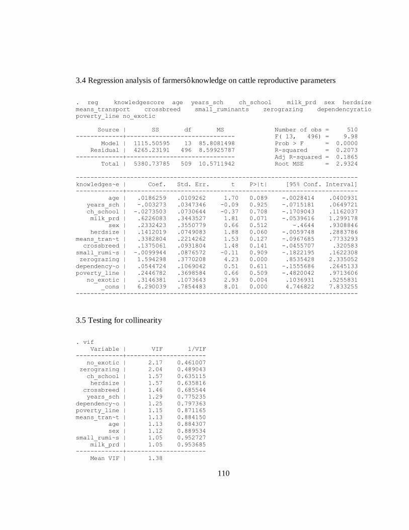
110
3.4 Regression analysis of farmers’ knowledge on cattle reproductive parameters
. reg knowledgescore age years_sch ch_school milk_prd sex herdsize means_transport crossbreed small_ruminants zerograzing dependencyratio poverty_line no_exotic Source | SS df MS Number of obs = 510 -------------+------------------------------ F( 13, 496) = 9.98 Model | 1115.50595 13 85.8081498 Prob > F = 0.0000 Residual | 4265.23191 496 8.59925787 R-squared = 0.2073 -------------+------------------------------ Adj R-squared = 0.1865 Total | 5380.73785 509 10.5711942 Root MSE = 2.9324 ------------------------------------------------------------------------------ knowledges~e | Coef. Std. Err. t P>|t| [95% Conf. Interval] -------------+---------------------------------------------------------------- age | .0186259 .0109262 1.70 0.089 -.0028414 .0400931 years_sch | -.003273 .0347346 -0.09 0.925 -.0715181 .0649721 ch_school | -.0273503 .0730644 -0.37 0.708 -.1709043 .1162037 milk_prd | .6226083 .3443527 1.81 0.071 -.0539616 1.299178 sex | .2332423 .3550779 0.66 0.512 -.4644 .9308846 herdsize | .1412019 .0749083 1.88 0.060 -.0059748 .2883786 means_tran~t | .3382804 .2214262 1.53 0.127 -.0967685 .7733293 crossbreed | .1375061 .0931804 1.48 0.141 -.0455707 .320583 small_rumi~s | -.0099944 .0876572 -0.11 0.909 -.1822195 .1622308 zerograzing | 1.594298 .3770208 4.23 0.000 .8535428 2.335052 dependency~o | .0544724 .1069042 0.51 0.611 -.1555686 .2645133 poverty_line | .2446782 .3698584 0.66 0.509 -.4820042 .9713606 no_exotic | .3146381 .1073643 2.93 0.004 .1036931 .5255831 _cons | 6.290039 .7854483 8.01 0.000 4.746822 7.833255 ------------------------------------------------------------------------------
3.5 Testing for collinearity
. vif Variable | VIF 1/VIF -------------+---------------------- no_exotic | 2.17 0.461007 zerograzing | 2.04 0.489043 ch_school | 1.57 0.635115 herdsize | 1.57 0.635816 crossbreed | 1.46 0.685544 years_sch | 1.29 0.775235 dependency~o | 1.25 0.797363 poverty_line | 1.15 0.871165 means_tran~t | 1.13 0.884150 age | 1.13 0.884307 sex | 1.12 0.889534 small_rumi~s | 1.05 0.952727 milk_prd | 1.05 0.953685 -------------+---------------------- Mean VIF | 1.38

111
3.6 Testing for heteroskedasticity
. estat hettest Breusch-Pagan / Cook-Weisberg test for heteroskedasticity Ho: Constant variance Variables: fitted values of knowledgescore chi2(1) = 0.04 Prob > chi2 = 0.8498

112
Appendix 4 Ordinary least squares for milk production
4.1 Correlation of variables used in the estimation of milk production
pwcorr knowledgescore1 sex age years_sch ch_school no_exotic crossbreed small_r > uminants milk_prd poverty_line zerograzing, sig star(5) | knowle~1 sex age years_~h ch_sch~l no_exo~c crossb~d -------------+--------------------------------------------------------------- knowledges~1 | 1.0000 sex | 0.0460 1.0000 | 0.2955 age | 0.1280* -0.0656 1.0000 | 0.0035 0.1350 | years_sch | 0.1398* 0.2869* -0.1340* 1.0000 | 0.0014 0.0000 0.0022 | ch_school | -0.1481* 0.0841 0.0085 -0.0862* 1.0000 | 0.0007 0.0553 0.8464 0.0495 | no_exotic | 0.3391* 0.0520 0.0501 0.1886* -0.2027* 1.0000 | 0.0000 0.2362 0.2544 0.0000 0.0000 | crossbreed | -0.0093 0.0277 0.0194 0.0032 0.0568 -0.3477* 1.0000 | 0.8325 0.5288 0.6592 0.9423 0.1959 0.0000 | small_rumi~s | 0.1076* 0.0937* 0.0073 0.1675* -0.0566 0.0517 0.0742 | 0.0141 0.0326 0.8675 0.0001 0.1975 0.2390 0.0910 | milk_prd | 0.1267* -0.0115 -0.0125 0.0672 -0.0952* 0.1216* 0.0478 | 0.0038 0.7927 0.7768 0.1257 0.0300 0.0055 0.2761 | poverty_line | 0.1544* 0.1724* -0.0495 0.2556* -0.0295 0.1517* 0.0692 | 0.0004 0.0001 0.2599 0.0000 0.5024 0.0005 0.1152 | zerograzing | 0.3881* -0.0033 0.0920* 0.2446* -0.4815* 0.5653* -0.2103* | 0.0000 0.9393 0.0359 0.0000 0.0000 0.0000 0.0000 | | small_~s milk_prd povert~e zerogr~g -------------+------------------------------------ small_rumi~s | 1.0000 | | milk_prd | -0.0503 1.0000 | 0.2525 | poverty_line | 0.1027* 0.1230* 1.0000 | 0.0192 0.0050 | zerograzing | 0.0404 0.1431* 0.2033* 1.0000 | 0.3581 0.0011 0.0000

113
Pairwise correlation is significant at the 0.05 level
4.2 Regression analysis of transformed milk production model
regress MILK knowledgescore sex age years_sch ch_school no_exotic crossbreed small_ruminants milk_prd poverty_line zerograzing Source | SS df MS Number of obs = 518 -------------+------------------------------ F( 11, 506) = 12.96 Model | 1250.9192 11 113.719927 Prob > F = 0.0000 Residual | 4440.79027 506 8.77626535 R-squared = 0.2198 -------------+------------------------------ Adj R-squared = 0.2028 Total | 5691.70947 517 11.0091092 Root MSE = 2.9625 ------------------------------------------------------------------------------ MILK | Coef. Std. Err. t P>|t| [95% Conf. Interval] -------------+---------------------------------------------------------------- knowledges~e | 1.591962 .3359247 4.74 0.000 .9319833 2.251941 sex | -.2648511 .3554747 -0.75 0.457 -.9632392 .4335369 age | .0036227 .0105883 0.34 0.732 -.0171798 .0244251 years_sch | .0394899 .0343214 1.15 0.250 -.0279401 .1069199 ch_school | .0747564 .0680695 1.10 0.273 -.0589773 .20849 no_exotic | .2819084 .0945452 2.98 0.003 .096159 .4676579 crossbreed | .2727594 .0850641 3.21 0.001 .1056372 .4398816 small_rumi~s | .0583141 .0812242 0.72 0.473 -.1012641 .2178923 milk_prd | 1.266954 .3467129 3.65 0.000 .5857803 1.948128 poverty_line | .978524 .370564 2.64 0.009 .2504906 1.706557 zerograzing | .8251268 .3793584 2.18 0.030 .0798153 1.570438 _cons | -2.284734 .9390745 -2.43 0.015 -4.129699 -.4397685 ------------------------------------------------------------------------------
4.3 Test for collinearity
vif Variable | VIF 1/VIF -------------+---------------------- zerograzing | 2.07 0.483017 no_exotic | 1.68 0.596355 ch_school | 1.35 0.739675 years_sch | 1.26 0.796623 knowledges~e | 1.21 0.824441 crossbreed | 1.20 0.832907 poverty_line | 1.14 0.874907 sex | 1.13 0.888052 age | 1.06 0.940659 milk_prd | 1.06 0.941100 small_rumi~s | 1.05 0.948841 -------------+---------------------- Mean VIF | 1.29

114
4.4 Test for heteroskedasticity Hottest Breusch-Pagan / Cook-Weisberg test for heteroskedasticity Ho: Constant variance Variables: fitted values of MILK chi2(1) = 2.61 Prob > chi2 = 0.1063
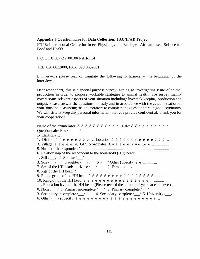
115
Appendix 5 Questionnaire for Data Collection: FAO/IFAD Project ICIPE: International Centre for Insect Physiology and Ecology - African Insect Science for Food and Health
P.O. BOX 30772 – 00100 NAIROBI
TEL: 020 8632000, FAX: 020 8632001
Enumerators please read or translate the following to farmers at the beginning of the interviews:
Dear respondent, this is a special purpose survey, aiming at investigating issue of animal production in order to propose workable strategies to animal health. The survey mainly covers some relevant aspects of your situation including: livestock keeping, production and output. Please answer the questions honestly and in accordance with the actual situation of your household, assisting the enumerators to complete the questionnaire in good conditions. We will strictly keep any personal information that you provide confidential. Thank you for your cooperation!
Name of the enumerator: …………………………… Date: ………………………… Questionnaire No: /______/ 1- Identification 1. Division……………………… 2. Location: ……………………………………... 3. Village: …………… 4. GPS coordinates: X = …………Y = …..…….................. 5. Name of the respondent….............................................................................................. 6. Relationship of the respondent to the household (HH) head: 1. Self /___/ 2. Spouse /___/ 3. Son /___/ 4. Daughter /___/ 5 /___/ Other (Specify) …….............. 7. Sex of the HH head: 1. Male /___/ 2. Female /___/ 8. Age of the HH head: /_______/ 9. Ethnic group of the HH head: ……………………………………………......... 10. Religion of the HH head: …………………………………………….............. 11. Education level of the HH head: (Please record the number of years at each level) 0. None /___/ 1. Primary incomplete /___/ 2. Primary complete /___/ 3. Secondary incomplete /___/ 4. Secondary complete /___/ 5. University /___/ 6. Other /___/ (Specify) ………………………………………………………..

116
12. Number of persons in the household /____/ Age Male Female Active Non active 0 to 5 years 6 years to 14 years 15 years to 64 years More than 64 years 13. How many children go to school? /____/ 14. How many Bikes, Motobikes and Cars do you have in the household? Bikes
Moto bikes Cars
2- Animal Production 2.1- Herd composition Categories Number Number owned by
female Calves 0 to 1year Male > 1 year Heifers Cows
2.2- Number of oxen if any/____/
2.3- Cow breed in the herd (including cows in Zero grazing)
Races Number Friesian Ayrshire Guernsey Boran Local Zebu Sahiwal Crossbreed
2.4- What are the reasons of the choice of the breed? Friesian :............................................................................................................................. Ayrshire:............................................................................................................................. Guernsey:.......................................................................................................................… Boran :........................................................................................................................…… Local Zebu:........................................................................................................................ Crossbreed......................................................................................................................... 2.5- How many sheep and goats do you have? /____/ Number owned by female /____/

117
2.6- What are the roles of cattle in the household? (Please rank the role) Role Rank Meat Production Milk Production Manure Production Saving Sale Animal traction Prestige
2.7- What are the signs do you use to detect heat on your cows? (Please rank the signs)
Signs Rank
2.8- At which age do you observe the first heat in your heifer? ....................................... 2.9- What is the duration from calving to the first heat? ................................................... 2.10- How many heats do you observe in your heifer before you call the inseminator? ... 2.11- How many heats do you observe after calving before you call the inseminator? .... 2.12- For reproduction what do you use? 1. Bull /___/ or 2.Artificial Insemination (AI /___/ 2.13- After how many hours do you serve your cow after detecting the heat? 1 to 2/___/ 2 to 4/___/ 4 to 6/___/ 6 to 8/___/ 8 to 10/___/ 10 to 12/___/ >12/___/ 2.14- How do you know that your cow is pregnant? (Please rank the signs) Signs Rank
2.15- What is the duration from calving to the conception? .............................................. 2.16- What is the gestation length? ................................................................................... 2.17- Do your cows ever have placenta retention during the last 12 months? 1 YES /___/ 2 NO /___/
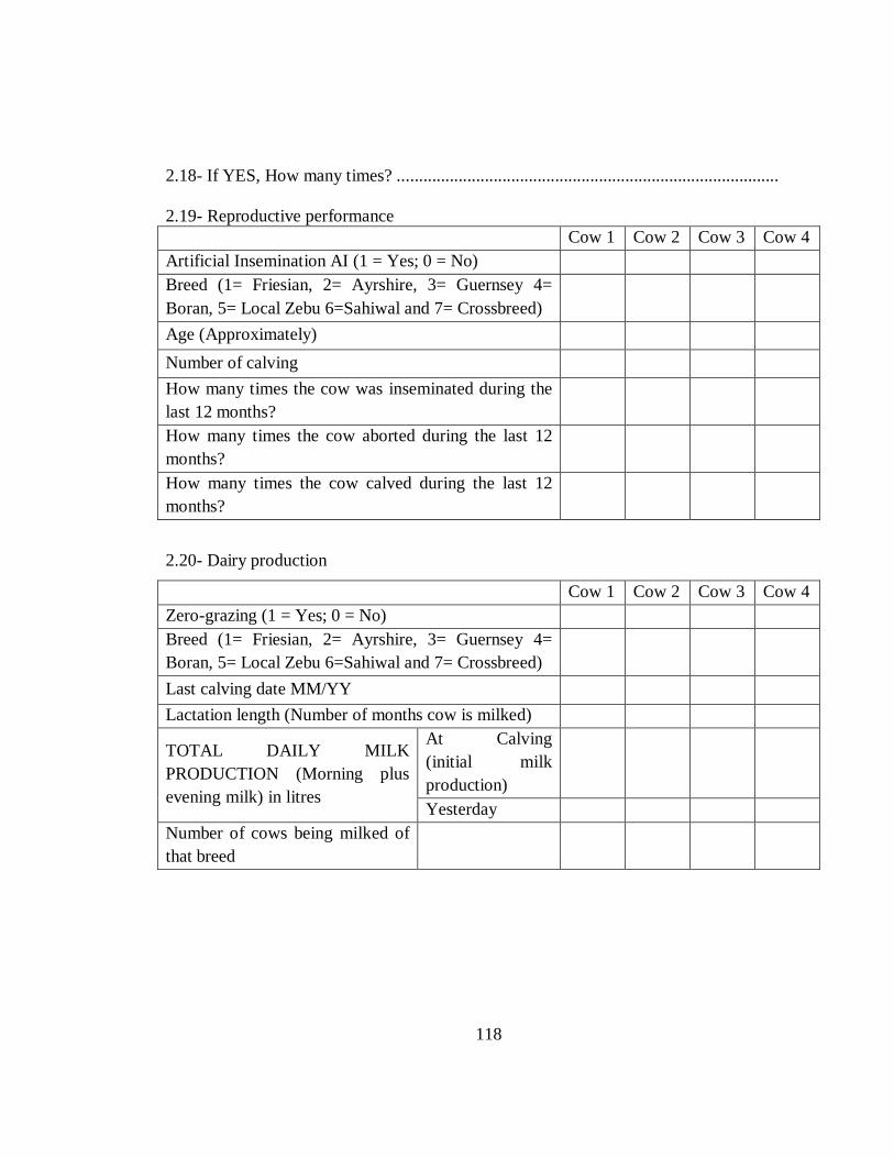
118
2.18- If YES, How many times? ....................................................................................... 2.19- Reproductive performance Cow 1 Cow 2 Cow 3 Cow 4 Artificial Insemination AI (1 = Yes; 0 = No) Breed (1= Friesian, 2= Ayrshire, 3= Guernsey 4= Boran, 5= Local Zebu 6=Sahiwal and 7= Crossbreed)
Age (Approximately) Number of calving How many times the cow was inseminated during the last 12 months?
How many times the cow aborted during the last 12 months?
How many times the cow calved during the last 12 months?
2.20- Dairy production
Cow 1 Cow 2 Cow 3 Cow 4 Zero-grazing (1 = Yes; 0 = No) Breed (1= Friesian, 2= Ayrshire, 3= Guernsey 4= Boran, 5= Local Zebu 6=Sahiwal and 7= Crossbreed)
Last calving date MM/YY Lactation length (Number of months cow is milked)
TOTAL DAILY MILK PRODUCTION (Morning plus evening milk) in litres
At Calving (initial milk production)
Yesterday Number of cows being milked of that breed

119
2.21- Cattle exists Have any cattle exited the household herd during the past 12 months. (0 = No, 1 = Yes, 2 = don’t know) [ ] If yes, fill in the below table. If sold Animal
type (*) How exited (**)
How many animals exited?
Purpose of selling (***)
Average price per animal Currency [ KSH ]
Where sold? (****)
Who controls the money? (*****)
1 2 3 4 5 Coding for ANIMAL TYPE (*)
Coding for HOW EXITED (**)
Coding for PURPOSE OF SELLING (***)
Coding for WHERE SOLD (****)
Coding for WHO CONTROLS THE MONEY? (*****)
1= calve 2= Male > 1 year 3= Heifers 4= Cows 5= oxen
1=Sale (live animals) 2=Died, lost or stolen 3=Slaughter for household needs 4= Given away Other: (specify in cell)
1=To meet planned household expenses 2=To meet emergency household expenses 3=Livestock trading as a business 4=Culling Other: (specify in cell)
1=Farm gate 2=Village market 3=Regional town or market 4= Abattoir / butchery Other: (specify in cell)
1= head 2= spouse 3= other female member 4= other male member 5= other, specify

120
2.22- Livestock entries: Cattle (Entry over the last 12 months)
Animal type (*)
How many of this type (number)
Means of entry (**)
1 2 3 4 5 Coding for ANIMAL TYPE (*) Coding for MEANS OF ENTRY (**) 1= calve 2= Male > 1 year 3= Heifers 4= Cows 5= oxen
1=Born into herd/ flock 2= Purchased 3= Gift/ inherited
2.23- Animal Traction
How many oxen are at work in your household
Number of months of work over the last 12 months
Number of days of work per month
Number of hours of work per day
Area cultivated (ha) over the last 12 months

121
2.24- Inputs (bought over the last 12 months)
Category Quantity Unit Price (KHS) Total (KHS) Artificial Insemination (AI) Preventive Trypanocides Curative Trypanocides Vaccines Antibiotics Anti-helminties Acaricides/Insecticides Vitamins Salts Feed bought Veterinary fees costs Labour cost for herding
2.25- Income
In which of the following categories do you estimate your total monthly household income,
from all farm activities, working members, business income, pensions and remittances from
elsewhere (tick).
Ksh per month Tick < 2,500 2,500 - 5,000 5,000 - 10,000 10,000 - 20,000 20,000 - 30,000 > 30,000

122
Appendix 6 Interviewer capturing responses from respondents
Interviewer capturing responses assisted by the Icipe field staff to interpret the responses
given by the respondent