analysis of failures of decoders for ldpc...
TRANSCRIPT

Analysis of Failures of Decoders for LDPC Codes
Item Type text; Electronic Dissertation
Authors Chilappagari, Shashi Kiran
Publisher The University of Arizona.
Rights Copyright © is held by the author. Digital access to this materialis made possible by the University Libraries, University of Arizona.Further transmission, reproduction or presentation (such aspublic display or performance) of protected items is prohibitedexcept with permission of the author.
Download date 31/05/2018 10:43:07
Link to Item http://hdl.handle.net/10150/195483
ANALYSIS OF FAILURES OF DECODERS FOR LDPC CODES
by
Shashi Kiran Chilappagari
A Dissertation Submitted to the Faculty of the
DEPARTMENT OF ELECTRICAL AND COMPUTER ENGINEERING
In Partial Fulfillment of the Requirements
For the Degree of
DOCTOR OF PHILOSOPHY
In the Graduate College
THE UNIVERSITY OF ARIZONA
2 0 0 8

2
THE UNIVERSITY OF ARIZONAGRADUATE COLLEGE
As members of the Dissertation Committee, we certify that we have read the
dissertation prepared by Shashi Kiran Chilappagari
entitled Analysis of Failures of Decoders for LDPC Codes
and recommend that it be accepted as fulfilling the dissertation requirement for the
Degree of Doctor of Philosophy
Date: November 12, 2008Bane Vasic, Ph.D.
Dissertation Director
Date: November 12, 2008Michael W. Marcellin, Ph.D.
Date: November 12, 2008William E. Ryan, Ph.D.
Date: November 12, 2008Kalus M. Lux, Ph.D.
Final approval and acceptance of this dissertation is contingent upon the candidate’s
submission of the final copies of the dissertation to the Graduate College.
I hereby certify that I have read this dissertation prepared under my direction and
recommend that it be accepted as fulfilling the dissertation requirement.
Date: November 12, 2008
Dissertation Director: Bane Vasic, Ph.D.

3
STATEMENT BY AUTHOR
This dissertation has been submitted in partial fulfillment of requirements for an
advanced degree at The University of Arizona and is deposited in the University
Library to be made available to borrowers under rules of the Library.
Brief quotations from this dissertation are allowable without special permission,
provided that accurate acknowledgment of source is made. Requests for permission
for extended quotation from or reproduction of this manuscript in whole or in part
may be granted by the head of the major department or the Dean of the Graduate
College when in his or her judgment the proposed use of the material is in the
interests of scholarship. In all other instances, however, permission must be obtained
from the author.
SIGNED:
Shashi Kiran Chilappagari

4
ACKNOWLEDGEMENTS
I consider it my extreme good fortune to have Prof. Bane Vasic as my Ph.D. advisor.
Over the past four and a half years, Dr. Vasic has been an excellent mentor who
has inspired and motivated me to pursue excellence in all of my endeavors. His
immense knowledge in a vast number of topics, his deep passion for research and
his personal interest in my welfare have contributed greatly to the shaping of my
doctoral studies. I look forward to continuing my collaboration with him and benefit
from his wisdom.
I owe a great debt of gratitude to Prof. Michael W. Marcellin for his excellent
teaching as well as his invaluable guidance all through my Ph.D. studies. Special
thanks to Prof. Kalus Lux for taking interest in my research and inspiring me
with his refreshing approach toward teaching and research. I would like to thank
Prof. William Ryan for his valuable guidance. I would also like to thank Prof. Ivan
Djordevic for very valuable discussions. I would also like to acknowledge the financial
support of the National Science Foundation and the Information Storage Industry
Consortium. My sincere thanks to the ECE staff, particularly, Tami, Nancy and
Caroll, who have been very helpful by taking care of all the paperwork.
During the past four years, I have had the honor of working with many experts
in coding theory and I wish to express my thanks to Dr. Misha Chertkov for giving
me an opportunity to work at the Los Alamos national Laboratory, Dr. Evagelos
Eleftheriou for providing me with an opportunity to intern at IBM, Zurich, and
Dr. David Declercq for inviting me to ENSEA, Paris, France. I wish to thank
Dr. Thomas Mittelholzer and Dr. Sedat Oelcer for their guidance during my stay

5
at IBM. My sincere thanks to Dr. Olgica Milenkovic for her valuable suggestions
during the early part of my Ph.D. studies.
Many teachers over the past decade have been instrumental in shaping my career
and while I cannot possibly list all of them, I would like to specifically mention Prof.
V. V. Rao, who taught me the basics of coding theory and Prof. R. Arvind for his
encouragement. Four terrific teachers who have had a lasting impact on me are
Ramaiah sir, Koteshwar Rao sir, Madhusudan sir and Surendranath sir, and no
amount of praise can justify the gratitude I owe to them.
Working with my lab mates has been a lot of fun and I could not have asked
for better collaborators than Sundar, Rathna, Milos, Ananth, Dung and Shiva. Life
in the desert was made bearable by the many cool friends I have made here and
I take this opportunity to thank all of them, especially Hari, Rahul and Sarika. I
would also like to thank my longtime friends Raghuram, Pavan, Pavanram, Vamsi,
Surender and Sujana who have always supported and encouraged me.
Finally, I would like to thank all my family members for their unwavering sup-
port. My thanks to my in-laws for their understanding. Special thanks to my elder
sister, Sravanthi, and my brother-in-law, Raghu, have always been there for me and
my little niece, Rushika (who probably does not yet understand what Ph.D. means)
who has brought joy to the entire family. Thanks to my younger sister Pallavi who
has always been a source of support and encouragement. A lot of credit for the
completion of my dissertation goes to my wife Swapna, and I take this opportunity
to acknowledge her support. Above all, I wish to thank my mom and dad who have
made many sacrifices to provide us with the best of things, who taught me the value
of education, and who have always stood by me with their unconditional love.

6
DEDICATION
To
Swapna, of course
And
Other family members

7
TABLE OF CONTENTS
LIST OF FIGURES . . . . . . . . . . . . . . . . . . . . . . . . . . . . 10
LIST OF TABLES . . . . . . . . . . . . . . . . . . . . . . . . . . . . . 13
ABSTRACT . . . . . . . . . . . . . . . . . . . . . . . . . . . . . . . . . 14
CHAPTER 1 Introduction . . . . . . . . . . . . . . . . . . . . . . . . 16
1.1 Historical Background . . . . . . . . . . . . . . . . . . . . . . . . . . 16
1.2 Motivation and Problem Background . . . . . . . . . . . . . . . . . . 19
1.3 Contributions of this Dissertation . . . . . . . . . . . . . . . . . . . . 24
1.4 Organization of the Dissertation . . . . . . . . . . . . . . . . . . . . . 25
CHAPTER 2 Preliminaries . . . . . . . . . . . . . . . . . . . . . . . 26
2.1 LDPC Codes . . . . . . . . . . . . . . . . . . . . . . . . . . . . . . . 26
2.2 Channel Assumptions . . . . . . . . . . . . . . . . . . . . . . . . . . . 29
2.3 Decoding Algorithms . . . . . . . . . . . . . . . . . . . . . . . . . . . 31
2.3.1 Message Passing Decoders . . . . . . . . . . . . . . . . . . . . 31
2.3.2 Bit Flipping Decoders . . . . . . . . . . . . . . . . . . . . . . 34
2.3.3 Linear Programming Decoder . . . . . . . . . . . . . . . . . . 35
2.4 Decoder Failures . . . . . . . . . . . . . . . . . . . . . . . . . . . . . 36
2.4.1 Trapping Sets for Iterative Decoders . . . . . . . . . . . . . . 37
2.4.2 Pseudo-codewords for LP decoders . . . . . . . . . . . . . . . 39

TABLE OF CONTENTS – Continued
8
2.5 Error Correction Capability and Slope of the FER Curve . . . . . . . 41
CHAPTER 3 Error Correction Capability of Column-Weight-Three
Codes: I . . . . . . . . . . . . . . . . . . . . . . . . . . . . . . . . . 43
3.1 Conditions for a Fixed Set . . . . . . . . . . . . . . . . . . . . . . . . 43
3.2 Girth of Tanner Graph and Size of Inducing Sets . . . . . . . . . . . 46
3.3 Proofs . . . . . . . . . . . . . . . . . . . . . . . . . . . . . . . . . . . 49
3.3.1 Proof of Lemma 3.3.(i) . . . . . . . . . . . . . . . . . . . . . . 49
3.3.2 Proof of Lemma 3.3.(ii) . . . . . . . . . . . . . . . . . . . . . . 49
3.3.3 Proof of Lemma 3.3.(iii) . . . . . . . . . . . . . . . . . . . . . 50
3.3.4 Proof of Lemma 3.3.(iv) . . . . . . . . . . . . . . . . . . . . . 52
CHAPTER 4 Error Correction Capability of Column-Weight-Three
Codes: II . . . . . . . . . . . . . . . . . . . . . . . . . . . . . . . . . 55
4.1 Notation . . . . . . . . . . . . . . . . . . . . . . . . . . . . . . . . . . 56
4.2 The first l iterations . . . . . . . . . . . . . . . . . . . . . . . . . . . 57
4.3 Girth of Tanner Graph and Guaranteed Error Correction Capability . 62
4.3.1 g/2 is even . . . . . . . . . . . . . . . . . . . . . . . . . . . . . 62
4.3.2 g/2 is odd . . . . . . . . . . . . . . . . . . . . . . . . . . . . . 71
CHAPTER 5 Error Correction Capability of Higher Column Weight
Codes . . . . . . . . . . . . . . . . . . . . . . . . . . . . . . . . . . . 74
5.1 Expansion and Error Correction Capability . . . . . . . . . . . . . . . 75
5.2 Column Weight, Girth and Expansion . . . . . . . . . . . . . . . . . . 76

TABLE OF CONTENTS – Continued
9
5.2.1 Definitions . . . . . . . . . . . . . . . . . . . . . . . . . . . . . 76
5.2.2 The Main Theorem . . . . . . . . . . . . . . . . . . . . . . . . 79
5.3 Cage Graphs and Trapping Sets . . . . . . . . . . . . . . . . . . . . . 81
CHAPTER 6 Applications and Numerical Results . . . . . . . . . 85
6.1 Trapping Set Statistics for Different Codes . . . . . . . . . . . . . . . 85
6.2 Instanton Statistics for LP Decoding over the BSC . . . . . . . . . . 86
6.3 Code Construction Avoiding Certain Topological Structures . . . . . 89
CHAPTER 7 Concluding Remarks . . . . . . . . . . . . . . . . . . . 93
APPENDIX A Column-Weight-Three Codes with Tanner Graphs of
Girth Less Than 10 . . . . . . . . . . . . . . . . . . . . . . . . . . . 96
A.1 The Case of Codes with Tanner Graphs of Girth Eight . . . . . . . . 97
APPENDIX B Finding Instantons for LP Decoding Over the BSC 106
B.1 Instanton Search Algorithm and its Analysis . . . . . . . . . . . . . . 109
REFERENCES . . . . . . . . . . . . . . . . . . . . . . . . . . . . . . . 114

10
LIST OF FIGURES
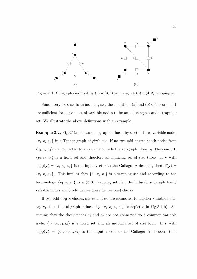
3.1 Subgraphs induced by (a) a (3, 3) trapping set (b) a (4, 2) trapping set 45
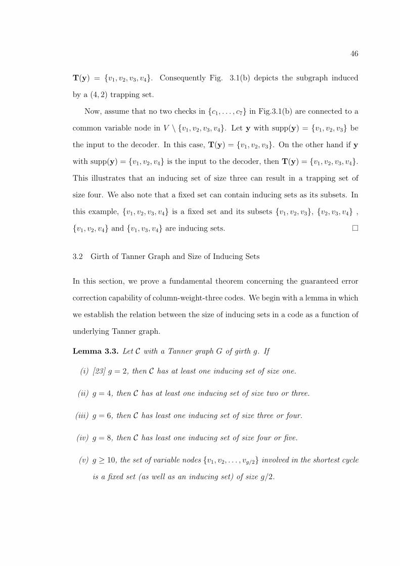
3.2 Illustration of a cycle of length g . . . . . . . . . . . . . . . . . . . . 47
3.3 Subgraphs induced by (a) a (4, 4) trapping set (b) a (5, 3) trapping set 53
4.1 Possible configurations of at most 2l + 1 bad variable nodes in the
neighborhood of a variable node v sending an incorrect message to
check node c in the (l + 1)th iteration for (a) l = 1, (b) l = 2 and (c)
l = 3. . . . . . . . . . . . . . . . . . . . . . . . . . . . . . . . . . . . 60
4.2 Configurations of at most 7 bad variable nodes, free of cycles of length
less than 16, which do not converge in 4 iterations. . . . . . . . . . . 64
4.3 Construction of Cg−4 from Cg . . . . . . . . . . . . . . . . . . . . . . . 65
4.4 Construction of Cg+4 from Cg. . . . . . . . . . . . . . . . . . . . . . . 66
4.5 Configurations of at most 2l + 1 bad variable nodes free of cycles of
length less than 4l + 4 which do not converge in (l + 1) iterations. . . 67
4.6 Configurations of at most 5 variable nodes free of cycles of length less
than 12 which do not converge in 3 iterations. . . . . . . . . . . . . . 70
4.7 (a) Configuration of at most 6 bad variable nodes free of cycles of
length less than 14 which does not converge in 4 iterations (b) Con-
figuration of at most 2l bad variable nodes free of cycles of length less
than 4l + 2 which does not converge in l + 1 iterations. . . . . . . . . 72

LIST OF FIGURES – Continued
11
4.8 Configurations of at most 4 variable nodes free of cycles of length less
than 10 which do not converge in 3 iterations. . . . . . . . . . . . . . 73
6.1 FER plots for different codes (a) MacKay’s random code one (b) The
Margulis code (c) The Tanner code . . . . . . . . . . . . . . . . . . . 87
6.2 Frequency of instanton (ISA outputs) sizes for different weights of
inputs. (Total length of the bars (for any of the sub-plots) should sum
to one.) The bar-graphs were obtained by running the ISA for 2000
different random initiations with the fixed number of flips (ranging
from 16 to 30). Numbers at zero (if any) show the frequency of
patterns decoded into the all-zero-codeword. . . . . . . . . . . . . . . 88
6.3 Instanton-Bar-Graph showing the number of unique instantons of a
given weight found by running the ISA with 20 random flips for 2000
and 5000 initiations respectively. . . . . . . . . . . . . . . . . . . . . . 90
6.4 FER performance of the Tanner code and the new code. . . . . . . . 92
6.5 Instanton weight distribution for the Tanner code and the new code
for LP decoding over the BSC as found by running the ISA 2000 times. 92
A.1 Illustration of message passing for a (5, 3) trapping set: (a) variable to
check messages in round one; (b) check to variable messages in round
one; (c) variable to check messages in round two; and (d) check to
variable messages in round two. Arrow-heads indicate the messages
with value 1. . . . . . . . . . . . . . . . . . . . . . . . . . . . . . . . . 98

LIST OF FIGURES – Continued
12
A.2 All the possible subgraphs that can be induced by three variable nodes
in a column-weight-three code . . . . . . . . . . . . . . . . . . . . . . 99
B.1 Squares represent pseudo-codewords and circles represent medians
or related noise configurations (a) LP decodes median of a pseudo-
codeword into another pseudo-codeword of smaller weight (b) LP
decodes median of a pseudo-codeword into another pseudo-codeword
of the same weight (c) LP decodes median of a pseudo-codeword
into the same pseudo-codeword (d) Reduced subset (three different
green circles) of a noise configuration (e.g. of a median from the
previous step of the ISA) is decoded by the LP decoder into three
different pseudo-codewords (e) LP decodes the median (blue circle)
of a pseudo-codeword (low red square) into another pseudo-codeword
of the same weight (upper red square). Reduced subset of the median
(three configurations depicted as green circles are all decoded by LP
into all-zero-codeword. Thus, the median is an instanton. . . . . . . . 110
13
LIST OF TABLES
6.1 Different Codes and Their Parameters . . . . . . . . . . . . . . . . . 86

14
ABSTRACT
Ever since the publication of Shannon’s seminal work in 1948, the search for capacity
achieving codes has led to many interesting discoveries in channel coding theory.
Low-density parity-check (LDPC) codes originally proposed in 1963 were largely
forgotten and rediscovered recently. The significance of LDPC codes lies in their
capacity approaching performance even when decoded using low complexity sub-
optimal decoding algorithms. Iterative decoders are one such class of decoders that
work on a graphical representation of a code known as the Tanner graph. Their
properties have been well understood in the asymptotic limit of the code length
going to infinity. However, the behavior of various decoders for a given finite length
code remains largely unknown.
An understanding of the failures of the decoders is vital for the error floor analysis
of a given code. Broadly speaking, error floor is the abrupt degradation in the frame
error rate (FER) performance of a code in the high signal-to-noise ratio domain.
Since the error floor phenomenon manifests in the regions not reachable by Monte-
Carlo simulations, analytical methods are necessary for characterizing the decoding
failures. In this work, we consider hard decision decoders for transmission over the
binary symmetric channel (BSC).
For column-weight-three codes, we provide tight upper and lower bounds on the
guaranteed error correction capability of a code under the Gallager A algorithm
as a function of the girth of the underlying Tanner graph. We accomplish this by

15
studying combinatorial objects known as trapping sets. For higher column weight
codes, we establish bounds on the minimum number of variable nodes that achieve
certain expansion as a function of the girth of the underlying Tanner graph, thereby
obtaining lower bounds on the guaranteed error correction capability. We explore
the relationship between a class of graphs known as cage graphs and trapping sets
to establish upper bounds on the error correction capability.
We also propose an algorithm to identify the most probable noise configurations,
also known as instantons, that lead to error floor for linear programming (LP)
decoding over the BSC. With the insight gained from the above analysis techniques,
we propose novel code construction techniques that result in codes with superior
error floor performance.

16
CHAPTER 1
Introduction
If I have seen a little further it is by standing on the shoulders of Giants.
Sir Isaac Newton
1.1 Historical Background
As with any dissertation in information theory, we begin the historical background
of coding and information theory with Shannon’s work first published in 1948 [1].
Shannon proved that every communication channel has an associated capacity, and
that reliable communication is possible at all rates up to the capacity and for com-
munication at any rate above the capacity, the probability of error is bounded away
from zero. Specifically, he showed that for all rates below the capacity, there exist
a channel code and a decoding algorithm for which the probability of error can be
made as small as possible. Shannon, however, did not provide explicit construction
of such codes and since then the search for capacity achieving codes has led to many
developments in the area of coding theory.
The initial developments in channel coding had a strong algebraic flavor, high-
lighted in the seminal work of Hamming [2] who was the first to propose linear
block codes capable of correcting a single error. Hamming’s work was followed by
the discovery of multi-error correcting Bose-Chaudhuri-Hocquenghem (BCH) codes
by Hocquenghem [3] and Bose and Ray-Chaudhuri [4]. Reed and Solomon [5] then

17
proposed the now ubiquitous Reed-Solomon (RS) codes, which are a special class of
BCH codes. Efficient encoding and decoding algorithms for these codes that exploit
the underlying algebraic structure have been studied in great detail [6]. Algebraic
codes returned to the center of attention recently by the discovery of the so called
list decoding algorithms by Sudan [7], which also allow soft-decision decoding of
algebraic codes [8]. A more probabilistic flavor of channel coding can be found in
the area of convolutional codes [6], which are generally decoded using the Viterbi
algorithm [9]. However, both the above avenues did not lead to the construction of
capacity approaching codes with low-complexity decoding algorithms.
The quest for capacity achieving codes bore fruit with the discovery of Turbo
codes by Berrou, Glavieux, and Thitimajshima [10]. This was subsequently followed
by the renaissance of low-density parity-check (LDPC) codes in the last decade.
Gallager [11] proposed LDPC codes in his thesis which were largely forgotten for
the next three decades, with Tanner’s work [12] being the notable exception in
which he laid the foundations for the study of codes based on graphs. MacKay [13]
rediscovered LDPC codes and proved that there exist LDPC codes which achieve
capacity under the sum-product algorithm. A wide variety of algorithms known in
the areas of artificial intelligence, signal processing and digital communications can
be derived as specific instances of the sum-product algorithm (the interested reader
is referred to [14] for an excellent tutorial on this subject).
The significance of LDPC codes lies in their capacity approaching performance
even when decoded by sub-optimal low complexity algorithms. One class of such
decoders are the so-called iterative decoding algorithms, which include message-
passing algorithms (variants of the belief propagation algorithm [15] and Gallager

18
type algorithms [11]), and bit-flipping algorithms [16] (serial and parallel).
By generalizing the seminal work of Gallager [11] to ensembles of codes, Richard-
son and Urbanke [17] analyzed LDPC codes under message passing decoders and
showed that the bit error probability asymptotically tends to zero, whenever the
noise is below a finite threshold. The authors of [17] also proposed the density
evolution technique for computing the threshold and smaller signal-to-noise-ratio
(SNR) behavior of LDPC codes performing over different decoders and channels.
Richardson, Shokrollahi and Urbanke [18] used the density evolution approach for
code optimization, specifically to derive capacity approaching degree distributions
for irregular code ensembles. Bazzi, Richardson and Urbanke [19] derived exact
thresholds for the binary symmetric channel (BSC) and the Gallager A algorithm.
Zyablov and Pinsker [16] were the first to analyze LDPC codes under bit flipping
algorithms and demonstrated that regular LDPC codes with left degree greater than
four are capable of correcting a fraction of errors. Sipser and Spielman [20] analyzed
the bit flipping algorithms for LDPC codes using expansion based arguments. They
also proposed a general class of asymptotically good codes known as expander codes,
which were further analyzed and generalized by Barg and Zemor [21]. Burshtein and
Miller [22] applied expander based arguments to message passing algorithms to show
that these algorithms are also capable of correcting a fraction of errors. Recently,
Burshtein [23] showed a vast improvement in the fraction of correctable errors for
bit flipping algorithms.
The linear programming (LP) decoder is yet another sub-optimal decoder that
has gained prominence in the recent years mainly due to its amenability to analysis.
LP decoding was introduced by Feldman, Wainwright and Karger in [24] in which

19
they formulated the decoding problem as a linear program. Feldman and Stein
[25] showed that LP decoding achieves capacity on any binary-input memoryless
symmetric log-likelihood-ratio-bounded channel. Feldman et al. [26] used expander
arguments to show that LP decoding corrects a fraction of errors. Daskalakis, Di-
makis, Karp and Wainwright [27] considered probabilistic analysis of LP decoding
to establish better bounds on the fraction of correctable errors.
1.2 Motivation and Problem Background
A common feature of all the analysis methods used in deriving the asymptotic results
is that the underlying assumptions hold in the asymptotic limit of infinitely long code
and/or are applicable to an ensemble of codes. Hence, they are of limited use for the
analysis of a given finite length code. The performance of a code under a particular
decoding algorithm is characterized by the bit-error-rate (BER) or the frame-error-
rate (FER) curve plotted as a function of the SNR. A typical BER/FER vs SNR
curve consists of two distinct regions. At small SNR, the error probability decreases
rapidly with the SNR, with the curve looking like a water fall. The decrease slows
down at moderate values turning into the error-floor asymptotic at very large SNR
[28]. This transient behavior and the error-floor asymptotic originate from the sub-
optimality of the decoder, i.e., the ideal maximum-likelihood (ML) curve would
not show such a dramatic change in the BER/FER with the SNR increase. While
the slope of the BER/FER curve in the waterfall region is the same for almost all
the codes in the ensemble, there can be a huge variation in the slopes for different
codes in the error floor region [29]. Since for sufficiently long codes, the error floor
phenomenon manifests itself in the domain unreachable by brute force Monte-Carlo

20
simulations, analytical methods are necessary to characterize the FER performance.
Finite length analysis of LDPC codes is well understood for decoding over the
binary erasure channel (BEC). The decoder failures in the error floor domain are
governed by combinatorial structures known as stopping sets [30]. Stopping set
distributions of various LDPC ensembles have been studied by Orlitsky et al. (see
[31] and references therein for related works). Tian et al. [32] used this fact to
construct irregular LDPC codes which avoid small stopping sets thus improving
the guaranteed erasure recovery capability of codes under iterative decoding, and
hence improving the error-floors. Unfortunately, such a level of understanding of
the decoding failures has not been achieved for other important channels such as
the BSC and the additive white Gaussian noise channel (AWGNC).
Failures of iterative decoders for graph based codes were first studied by Wiberg
[33] who introduced the notions of computation trees and pseudo-codewords. Sub-
sequent analysis of the computation trees was carried out by Frey et al. [34] and
Forney et al. [35]. The failures of the LP decoder can be understood in terms of
the vertices of the so-called fundamental polytope which are also known as pseudo-
codewords. Vontobel and Koetter [36] introduced a theoretical tool known as the
graph cover decoding and used it to establish connections between the LP decoder
and the message passing decoders using the notion of the fundamental polytope.
They showed that the pseudo-codewords arising from the Tanner graph covers are
identical to the pseudo-codewords of the LP decoder. Vontobel and Koetter [37] also
studied the relation between the LP and min-sum decoders. The performance of the
min-sum decoder is governed by pseudo-codewords arising from computation-trees
as well as graph covers.

21
For iterative decoding on the AWGNC, MacKay and Postol [38] were the first
to discover that certain “near codewords” are to be blamed for the high error floor
in the Margulis code [39]. Richardson [28] reproduced their results and developed
a computation technique to predict the performance of a given LDPC code in the
error floor domain. He characterized the troublesome noise configurations leading
to error floor using combinatorial objects termed trapping sets and described a
technique (of a Monte-Carlo importance sampling type) to evaluate the error rate
associated with a particular class of trapping sets. The method from [28] was further
refined for the AWGN channel by Stepanov et al. [40] who introduced the notion
of instantons. In a nutshell, an instanton is a configuration of the noise which is
positioned between a codeword (say zero codeword) and another pseudo-codeword
(which is not necessarily a codeword). Incremental shift (allowed by the channel)
from this configuration toward the zero codeword leads to correct decoding (into the
zero-codeword) while incremental shift in an opposite direction leads to a failure.
In principle, one can find this dangerous configuration of the noise exploring the
domain of correct decoding surrounding the zero codeword, and finding borders of
this domain – the so-called error-surface. If the channel is continuous, the error-
surface consists of continuous patches while configuration of the noise maximizing
the error-probability over a patch is called an instanton.
As stated above, the instantons that affect the decoder performance in the error
floor region are extremely rare, and hence identifying and enumerating them is a
challenging task. However once this difficulty is overcome, the knowledge of the
trapping set/pseudo-codeword distribution can be used to evaluate the performance
of the code. It can also be used to guide optimization of the code and design

22
improved decoding strategies.
Previous investigation of the problem includes the work by Kelley and Sridhara
[41] who studied pseudo-codewords arising from graph covers and derived bounds
on the minimum pseudo-codeword weight in terms of the girth and the minimum
left-degree of the underlying Tanner graph. The bounds were further investigated
by Xia and Fu [42]. Smarandache and Vontobel [43] found pseudo-codeword distri-
butions for the special cases of codes from Euclidean and projective planes. Pseudo-
codeword analysis has also been extended to the convolutional LDPC codes by
Smarandache et al. [44]. Milenkovic et al. [45] studied the asymptotic distribution
of trapping sets in regular and irregular LDPC code ensembles. Wang et al. [46]
proposed an algorithm to exhaustively enumerate certain stopping and trapping
sets.
Chernyak et al. [47] and Stepanov et al. [40] suggested to pose this problem of
finding the instantons as a special optimization problem. This optimization method
was built in the spirit of the general methodology, borrowed from statistical physics,
guiding exploration of rare events which contribute the most to the BER/FER. The
optimization method allowed to discover in [40], the set of most probable instantons
for AWGN channel and iterative decoder. The operational utility of the method was
illustrated on some number of moderate size examples and strong dependence of the
instanton structure on the number of iterations was observed. The general optimiza-
tion method was substantially improved and refined in [48] for the LP decoding over
continuous channels (with main enabling example chosen to be the AWGNC). The
pseudo-codeword-search algorithm of [48] was essentially exploring in an iterative
way the Wiberg formula treating an instanton configuration as a median between a

23
pseudo-codeword and the zero-codeword. It was shown empirically that, initiated
with a sufficiently noisy configuration, the algorithm converges to an instanton in
sufficiently small number of steps, independent or weakly dependent on the code
size. Repeated multiple times the method outputs the set of instanton configu-
rations which can further be used to estimate the BER/FER performance in the
transient and error-floor domain. (See also [49] for an exhaustive list of references
for this and related subjects.)
An important outcome of all the work on error floors is the observation that
the slope of the FER curve of a given code under hard decision decoding in the
error floor region is related to the guaranteed error correction capability of the
code. Hence, in this dissertation, we focus primarily on establishing lower and
upper bounds on the number of errors that a decoding algorithm is guaranteed to
correct. To this end, we primarily consider hard decision decoding algorithms but
note that the general concepts are applicable to a wide variety of channels and
decoding algorithms. Expander based arguments [20] provide the required lower
bounds as it is known that a variety of decoding algorithms can correct a fixed
fraction of errors if the underlying Tanner graph of a code is a good expander. It
is well known that a random graph is a good expander with high probability [20],
but the fraction of nodes having the required expansion is very small and hence
the code length to guarantee correction of a fixed number of errors must be large.
Moreover, determining the expansion of a given graph is known to be NP hard
[50], and spectral gap methods cannot guarantee an expansion factor of more than
1/2 [20]. Also, expander based arguments cannot be applied to codes with column
weight three, which are of interest in many practical scenarios owing to their low

24
decoding complexity. The approach in this dissertation is, therefore, to identify
and analyze the failures of different hard decision decoding iterative algorithms for
LDPC codes as a function of two important code parameters, namely column weight
and girth of the underlying graph, which are easy to determine for any given code.
1.3 Contributions of this Dissertation
• We prove that a necessary condition for a column-weight-three code to correct
all error patterns with up to q ≥ 5 errors is to avoid all cycles up to length 2q
in its Tanner graph representation. As a result, we prove that given α > 0,
at sufficiently large lengths, no code in the ensemble of regular codes with
column weight three can correct α fraction of errors. These results have been
reported in [51].
• We prove that a column-weight-three LDPC code with Tanner graph of girth
g ≥ 10 can correct all error patterns with up to g/2 − 1 errors under the
Gallager A algorithm. This result, in conjunction with the necessary condition
mentioned above, completely determines the slope of the FER curve in the
error floor region. These results have been reported in [52].
• For higher column weight codes, we derive lower bounds on the number of
variable nodes that achieve sufficient expansion as a function of the column
weight and girth of the Tanner graph of the code. We also derive bounds
on the size of the smallest possible trapping sets thereby establishing upper
bounds on the guaranteed error correction capability. These results have been
reported in [53].

25
• We illustrate how the knowledge of trapping sets can be used for (a) deriving
trapping set/pseudo-codeword statistics for hard decision decoders and (b)
construction of codes with superior error floor performance. These results
have been reported in [54, 55, 56].
1.4 Organization of the Dissertation
In Chapter 2, we establish the notation and provide necessary background. We
derive upper bounds and lower bounds on the error correction capability of column-
weight-three codes under the Gallager A algorithm in Chapter 3 and Chapter 4
respectively. Expansion properties of Tanner graphs with higher column weight
as a function of girth are derived in Chapter 5. We highlight the applications of
the knowledge of trapping sets with illustrative numerical results in Chapter 6 and
conclude with a few remarks in Chapter 7.

26
CHAPTER 2
Preliminaries
We could, of course, use any notation we want; do not laugh at notations;
invent them, they are powerful. In fact, mathematics is, to a large extent,
invention of better notations.
Richard P. Feynman (1963)
In this chapter, we provide a brief description of some fundamental concepts from
coding theory. We start with a description of block codes and then proceed to define
LDPC codes. We then discuss channel assumptions and decoding algorithms. We
then proceed to describe decoding failures in general and highlight the importance
of correction of a fixed number of errors and its relation to slope of the FER curve.
2.1 LDPC Codes
Definition 2.1. (Codes) We consider binary codes in this work.
• (Block Code) An (n, k) binary block code maps a message block of k infor-
mation bits to a binary n-tuple. The rate r of the code is given by r = k/n.
• (Linear Block Code) An (n, k) binary linear block code, C, is a subspace of
GF(2)n of dimension k.

27
• (Parity-Check Matrix) A parity check matrix H of C is a matrix whose
columns generate the orthogonal complement of C, i.e., an element x =
(x1, . . . , xn) of GF(2)n is a codeword of C iff xHT = 0.
Definition 2.2. (Graphs) We adopt the standard notation in graph theory (see
[57] for example).
• (Graph) A graph with set of nodes U and set of edges E is denoted by
G = (U,E). When there is no ambiguity, we simply denote the graph by G.
The order of the graph is |U | and the size of the graph is |E|.
• (Neighborhood) An edge e is an unordered pair {u1, u2} of nodes and is
said to be incident on u1 and u2. Two nodes u1 and u2 are said to be adjacent
(neighbors) if there is an edge incident on them. The set of all neighbors of a
node u is denoted by N (u).
• (Degree of a node) The degree of u, d(u), is the number of its neighbors
i.e., d(u) = |N (u)|. A node with degree one is called a leaf or a pendant node.
A graph is d-regular if all the nodes have degree d. The average degree d of a
graph is defined as d = 2|E|/|U |.
• (Girth of a graph) The girth g(G) of a graph G, is the length of smallest
cycle in G. When there is no ambiguity about the graph under consideration,
we denote the girth simply by g.
• (Bipartite graph) G = (V ∪ C,E) denotes a bipartite graph with two sets
of nodes; variable (left) nodes V and check (right) nodes C and edge set E.
Nodes in V have neighbors only in C and vice versa. A bipartite graph is

28
said to be dv-left regular if all variable nodes have degree dv, dc-right regular
if all check nodes have degree dc and (dv, dc) regular if all variable nodes have
degree dv and all check nodes have degree dc. The girth of a bipartite graph
is even.
LDPC codes [11] are a class of linear block codes which can be defined by sparse
bipartite graphs [12].
Definition 2.3. (LDPC Codes and Tanner Graphs) Let G be a bipartite
graph with two sets of nodes: the set of variable nodes V with |V | = n and the set
of check nodes C with |C| = m. This graph defines a linear block code of length
n and dimension at least n − m in the following way: The n variable nodes are
associated with the n coordinates of codewords. A binary vector x = (x1, . . . , xn) is
a codeword if and only if for each check node, the modulo two sum of its neighbors
is zero. Such a graphical representation of an LDPC code is called the Tanner graph
[12] of the code. The adjacency matrix of G gives H, a parity check matrix of C.
It should be noted that the Tanner graph is not uniquely defined by the code
and when we say the Tanner graph of an LDPC code, we only mean one possible
graphical representation. In this work, • represents a variable node, � represents
an even degree check node and � represents an odd degree check node.
Definition 2.4. Code Ensembles
• (Regular LDPC Codes) A (dv, dc) regular LDPC code of length n denoted
by (n, dv, dc) has a Tanner graph with n variable nodes each of degree dv
and ndv/dc check nodes each of degree dc. This code has length n and rate
r ≥ 1 − dv/dc [11].

29
• (Ensemble) [17] The ensemble of Cn(dv, dc)of (dv, dc)-regular LDPC codes of
length n is defined as follows. Assign to each node dv or dc “sockets” according
to whether it is a variable node or a check node, respectively. Label the
variable and check sockets separately with the set [ndv] := {1, . . . , ndv} in some
arbitrary fashion. Pick a permutation π on ndv letters at random with uniform
probability from the set of all (ndv)! such permutations. The corresponding
(labeled) bipartite graph is then defined by identifying edges with pairs of
sockets and letting the set of such pairs be {(i, π(i)), i = 1, . . . , ndv}.
2.2 Channel Assumptions
We assume that a binary codeword x is transmitted over a noisy channel and is
received as y. The support of a binary vector x, denoted by supp(x), is defined as
the set of all variable nodes v ∈ V such that xv 6= 0.
Definition 2.5. Channels and Decoding
• (Channel) A channel is characterized by input alphabet X , output alphabet
Y and transition probability Pr(y|x), the probability that y ∈ Y is received
given that x ∈ X was sent.
• (MAP Decoding) The maximum a posteriori (MAP) decoding consists of
finding the codeword x ∈ C which maximizes Pr(x|y), the probability that x
was sent given that y is received.
• (ML Decoding) Under the assumption that all information words are equally
likely, this is equivalent to ML decoding which finds a codeword x maximizing
Pr(y|x).

30
• (Memoryless Channel) A memoryless channel is a channel which satisfies
Pr(y|x) =∏
v∈V
Pr(yv|xv).
Hence it can be characterized by Pr(yv|xv), v ∈ V , the probability that yv is
received given that xv was sent.
• (Log-Likelihood Ratio) The negative log-likelihood ratio (LLR) correspond-
ing to the variable node v ∈ V is given by
γv = log
(
Pr(yv|xv = 0)
Pr(yv|xv = 1)
)
.
• (BSC) The BSC is a binary input memoryless channel with output alphabet
{0, 1}. On the BSC with transition probability p, every transmitted bit xv ∈
{0, 1} is flipped 1 with probability p and is received as yv ∈ {0, 1}. Hence,
γv =
log(
1−pp
)
if yv = 0
log(
p1−p
)
if yv = 1
• (AWGN Channel) For the AWGN channel, we assume that each bit xv ∈
{0, 1} is modulated using binary phase shift keying (BPSK) and transmitted
as xv = 1− 2xv and is received as yv = xv + nv, where {nv} are i.i.d. N(0, σ2)
random variables. Hence, we have
γv =2yv
σ2.
1The event of a bit changing from 0 to 1 and vice-versa is known as flipping.

31
2.3 Decoding Algorithms
In this section, we describe various decoding algorithms for decoding LDPC codes.
We start with iterative decoders which can further be subdivided into message pass-
ing algorithms and bit flipping decoders. There is a wide variety of message passing
algorithms; Gallager A/B, sum-product and min-sum to name a few. We then
describe the LP decoder in the most general setting.
2.3.1 Message Passing Decoders
Message passing decoders operate by passing messages along the edges of the Tan-
ner graph representation of the code. Gallager in [11] proposed two simple binary
message passing algorithms for decoding over the BSC; Gallager A and Gallager B.
There exist a large number of message passing algorithms (sum-product algorithm,
min-sum algorithm, quantized decoding algorithms, decoders with erasures to name
a few) [17] in which the messages belong to a larger alphabet.
Every round of message passing (iteration) starts with the variable nodes sending
messages to their neighboring check nodes (first half of the iteration) and ends by
the check nodes sending messages to their neighboring variable nodes (second half
of the iteration). Let y = (y1, . . . , yn), an n-tuple be the input to the decoder. Let
ωj(v, c) denote the message passed by a variable node v ∈ V to its neighboring
check node c ∈ C in the jth iteration and j(c, v) denote the message passed by a
check node c to its neighboring variable node v. Additionally, let ωj(v, : ) denote
the set of all messages from v, ωj(v, : \c) denote the set of messages from v to all
its neighbors except to c and ωj( : , c) denote the set of all messages to c. The terms
ωj( : \v, c), j(c, v), j(c, : \v), j( : , v) and j( : \c, v) are defined similarly.
32
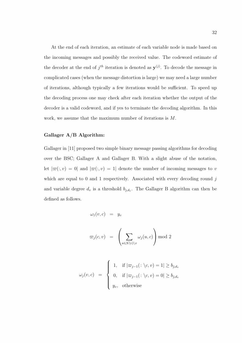
At the end of each iteration, an estimate of each variable node is made based on
the incoming messages and possibly the received value. The codeword estimate of
the decoder at the end of jth iteration is denoted as y(j). To decode the message in
complicated cases (when the message distortion is large) we may need a large number
of iterations, although typically a few iterations would be sufficient. To speed up
the decoding process one may check after each iteration whether the output of the
decoder is a valid codeword, and if yes to terminate the decoding algorithm. In this
work, we assume that the maximum number of iterations is M .
Gallager A/B Algorithm:
Gallager in [11] proposed two simple binary message passing algorithms for decoding
over the BSC; Gallager A and Gallager B. With a slight abuse of the notation,
let |(:, v) = 0| and |(:, v) = 1| denote the number of incoming messages to v
which are equal to 0 and 1 respectively. Associated with every decoding round j
and variable degree dv is a threshold bj,dv. The Gallager B algorithm can then be
defined as follows.
ω1(v, c) = yv
j(c, v) =
∑
u∈N (c)\v
ωj(u, c)
mod 2
ωj(v, c) =
1, if |j−1( : \c, v) = 1| ≥ bj,dv
0, if |j−1( : \c, v) = 0| ≥ bj,dv
yv, otherwise
33
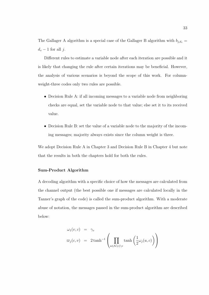
The Gallager A algorithm is a special case of the Gallager B algorithm with bj,dv=
dv − 1 for all j.
Different rules to estimate a variable node after each iteration are possible and it
is likely that changing the rule after certain iterations may be beneficial. However,
the analysis of various scenarios is beyond the scope of this work. For column-
weight-three codes only two rules are possible.
• Decision Rule A: if all incoming messages to a variable node from neighboring
checks are equal, set the variable node to that value; else set it to its received
value.
• Decision Rule B: set the value of a variable node to the majority of the incom-
ing messages; majority always exists since the column weight is three.
We adopt Decision Rule A in Chapter 3 and Decision Rule B in Chapter 4 but note
that the results in both the chapters hold for both the rules.
Sum-Product Algorithm
A decoding algorithm with a specific choice of how the messages are calculated from
the channel output (the best possible one if messages are calculated locally in the
Tanner’s graph of the code) is called the sum-product algorithm. With a moderate
abuse of notation, the messages passed in the sum-product algorithm are described
below:
ω1(v, c) = γv
j(c, v) = 2 tanh−1
∏
u∈N (c)\v
tanh
(
1
2ωj(u, c)
)

34
ωj(v, c) = γv +∑
u∈N (v)\c
j−1(u, v)
The codeword estimate at the end of j iterations is determined by the sign of m(j)v =
γv +∑
u∈N (v)
j(u, v). If m(j)v > 0 then y
(j)v = 0, otherwise y
(j)v = 1.
Min-Sum Algorithm
In the limit of high SNR, when the absolute value of the messages is large, the
sum-product becomes the min-sum algorithm, where the message from the check c
to the variable node v looks like:
j(c, v) = minu∈N (c)\v
∣
∣ωj(u, c)∣
∣ ·∏
u∈N (c)\v
sign(
ωj(u, c))
The min-sum algorithm has a property that the Gallager A/B and LP decoders
also possess — if we multiply all the likelihoods γv by a factor, all the decoding
would proceed as before and would produce the same result. Note that we don’t
have this “scaling” in the sum-product algorithm.
2.3.2 Bit Flipping Decoders
The bit flipping algorithms [16, 20] are iterative algorithms which do not belong to
the class of message passing algorithms. We now describe the parallel and serial bit
flipping algorithms. A constraint (check node) is said to be satisfied by a setting of
variable nodes if the sum of the variable nodes in the constraint is even; otherwise
the constraint is unsatisfied.

35
Parallel Bit Flipping Algorithm
• In parallel, flip each variable that is in more unsatisfied than satisfied con-
straints.
• Repeat until no such variable remains.
Serial Bit Flipping Algorithm
• If there is a variable that is in more unsatisfied than satisfied constraints, then
flip the value of that variable.
• Repeat until no such variable remains.
2.3.3 Linear Programming Decoder
The ML decoding of the code C allows a convenient LP formulation in terms of the
codeword polytope poly(C) whose vertices correspond to the codewords in C. The
ML-LP decoder finds f = (f1, . . . , fn) minimizing the cost function∑
v∈V
γvfv subject
to the f ∈ poly(C) constraint (see [24] for details). The formulation is compact but
impractical because of the number of constraints exponential in the code length.
Hence a relaxed polytope is defined as the intersection of all the polytopes as-
sociated with the local codes introduced for all the checks of the original code.
Associating (f1, . . . , fn) with bits of the code we require
0 ≤ fv ≤ 1, ∀v ∈ V (2.1)
For every check node c, let Ec = {T ⊆ N (c) : |T | is even}. The polytope Qc
associated with the check node c is defined as the set of points (f ,w) for which the

36
following constraints hold
0 ≤ wc,T ≤ 1, ∀T ∈ Ec (2.2)
∑
T∈Ec
wc,T = 1 (2.3)
fv =∑
T∈Ec,T∋v
wc,T , ∀v ∈ N (c) (2.4)
Now, let Q = ∩cQc be the set of points (f ,w) such that (2.1)-(2.4) hold for all
c ∈ C. (Note that Q, which is also referred to as the fundamental polytope [58, 36],
is a function of the Tanner graph G and consequently the parity-check matrix H
representing the code C.) The linear code linear program (LCLP) can be stated as
min(f ,w)
∑
v∈V
γvfv, s.t. (f ,w) ∈ Q.
For the sake of brevity, the decoder based on the LCLP is referred to in the following
as the LP decoder. A solution (f ,w) to the LCLP such that all fvs and wc,T s are
integers is known as an integer solution. The integer solution represents a codeword
[24]. It was also shown in [24] that the LP decoder has the ML certificate, i.e., if the
output of the decoder is a codeword, then the ML decoder would decode into the
same codeword. The LCLP can fail, generating an output which is not a codeword.
2.4 Decoder Failures
In this section, we define the various parameters needed to understand decoding fail-
ures. We deal with iterative decoders and LP decoders separately. To characterize
the performance of a coding/decoding scheme over any output symmetric channel,
one can assume, without loss of generality, the transmission of the all-zero-codeword,
i.e. x = 0. We make this assumption throughout the paper.
37
2.4.1 Trapping Sets for Iterative Decoders
Definition 2.6. (Trapping Sets [28]) Let y denote the input to the iterative
decoder and y(j) denote the codeword estimate of the decoder at the end of jth
iteration.
• A variable node v is said to be eventually correct if there exists a positive
integer lc such that for all lc ≤ j ≤ M , yjv = 0.
• For an input y, the failure set T(y) is defined as the set of variable nodes that
are not eventually correct. The decoding on the input y is successful if and
only if T(y) = ∅.
• If T(y) 6= ∅, then we say that T(y) is a trapping set. Since the failure sets of
two different input vectors can be the same trapping set, we denote a trapping
set simply by T . A trapping set T is said to be an (a, b) trapping set if it has
a variable nodes and b odd-degree check nodes in the sub-graph induced by
T .
Remark 2.7. An (a, b) trapping set is not unique i.e., two trapping sets with same
a and b can have different underlying topological structures (induced subgraphs).
So, when we talk of a trapping set, we refer to a specific topological structure. In
this paper, the induced subgraph is assumed to be known from the context.
Remark 2.8. In order to show that a given set of variable nodes T is a trapping
set, we should exhibit a vector y for which T(y) = T .
The definitions above do not provide the necessary and sufficient conditions for
a set of variable nodes to be a trapping set. Hence, for hard decision decoding
38
algorithms, we define the notion of a fixed set for which such conditions can be
derived and note that any fixed set is a trapping set.
Definition 2.9. (Inducing and Fixed Sets)
• Let y, a binary n-tuple, be the input to a hard decision decoder. If T(y) 6= ∅,
then we say that supp(y) is an inducing set. The size of an inducing set is its
cardinality.
• Let F be a set of variable nodes and let y with supp(y) = F be the input to
the Gallager A/B algorithm. If ωj(v, c) = yv, ∀j > 0, then F is known as a
fixed set and y is known as a fixed point.
• Let F be a set of variable nodes and let y with supp(y) = F be the input to
the bit flipping decoder (serial or parallel). F is a fixed set for the bit flipping
algorithms if the set of corrupt variables after every iteration is F .
When a fixed point is the input to the decoder then the messages passed from
variable nodes to check nodes along the edges are the same in every iteration. Since
the outgoing messages from variable nodes are same in every iteration, it follows
that the incoming messages from check nodes to variable nodes are also same in
every iteration and so is the estimate of a variable after each iteration. In fact, the
estimate after each iteration coincides with the received value. It is clear from the
above definition that if the input to the decoder is a fixed point, then the output of
the decoder is the same fixed point. It follows that for transmission over the BSC,
if y is a fixed point and T(y) 6= ∅, then T(y) = supp(y) is a trapping set as well as
an inducing set.

39
Definition 2.10. (Critical Number) Let T be a trapping and let y ∈ GF(2)n. Let
Y(T ) = {y|T(y) = T }. The critical number Tc of trapping set T for the Gallager
algorithm is the minimum number of variable nodes that have to be initially in error
for the decoder to end up in the trapping set T , i.e.,
Tc = minY(T )
|supp(y)|.
The most relevant trapping set in the error floor region is the trapping set with the
least critical number.
Definition 2.11. (Instanton) An instanton is a binary vector i such that T(i) = T
for some trapping set T and for any binary vector r such that supp(r) ⊂ supp(i),
T(i) = ∅. The size of an instanton is the cardinality of its support.
2.4.2 Pseudo-codewords for LP decoders
In contrast to the iterative decoders, the output of the LP decoder is well defined
in terms of pseudo-codewords.
Definition 2.12. (Pseudo-codewords [24]) Integer pseudo-codeword is a vector
p = (p1, . . . , pn) of non-negative integers such that, for every parity check c ∈ C,
the neighborhood {pv : v ∈ N(c)} is a sum of local codewords.
Alternatively, we can define a re-scaled pseudo-codeword, p = (p1, . . . , pn) where
0 ≤ pv ≤ 1, ∀v ∈ V , simply equal to the output of the LCLP. In the following, we
adopt the re-scaled definition.
We now define another important parameter, namely the cost associated with
LP decoding of a given vector to a pseudo-codeword.

40
Definition 2.13. The cost associated with LP decoding of a vector y to a pseudo-
codeword p is given by
C(y,p) =∑
v∈V
γvpv.
In the case of the BSC, the likelihoods are scaled as
γv =
1, if yv = 0;
−1, if yv = 1.
Hence, the cost associated with LP decoding of a binary vector r to a pseudo-
codeword p is given by
C(r,p) =∑
i/∈supp(r)
pi −∑
i∈supp(r)
pi. (2.5)
A given code C may have different Tanner graph representations and conse-
quently potentially different fundamental polytopes. Hence, we refer to the pseudo-
codewords as corresponding to a particular Tanner graph G of C.
Definition 2.14. (Pseudo-codeword Weight [41, Definition 2.10]) Let p =
(p1, . . . , pn) be a pseudo-codeword distinct from the all-zero-codeword of the code C
represented by Tanner graph G . Let q be the smallest number such that the sum
of the q largest pvs is at least
(
∑
v∈V
pv
)
/2. Then, the pseudo-codeword weight of p
is defined as follows:
• wBSC(p) for the BSC is
wBSC(p) =
2q, if∑
q
pv =
(
∑
v∈V
pv
)
/2;
2q − 1, if∑
q
pv >
(
∑
v∈V
pv
)
/2.

41
• wAWGN(p) for the AWGNC is
wAWGN(p) =(p1 + . . . + pn)2
(p21 + . . . + p2
n)
The minimum pseudo-codeword weight of G denoted by wBSC/AWGNmin is the min-
imum over all the non-zero pseudo-codewords of G.
Definition 2.15. (BSC Instanton) The BSC instanton i is a binary vector with
the following properties: (1) There exists a pseudo-codeword p such that C(i,p) ≤
C(i,0) = 0; (2) For any binary vector r such that supp(r) ⊂ supp(i), there exists
no pseudo-codeword with C(r,p) ≤ 0. The size of an instanton is the cardinality of
its support.
2.5 Error Correction Capability and Slope of the FER Curve
We establish the relation between the guaranteed error correction capability of
LDPC codes and the slope of the FER curve in the error floor region under hard
decision decoding algorithms.
Let p be the transition probability of the BSC and cr be the number of config-
urations of received bits for which r channel errors lead to codeword (frame) error.
The frame error rate (FER) is given by:
FER(p) =n∑
r=i
crpr(1 − p)(n−r)
where i is the minimal number of channel errors that can lead to a decoding error
and n is length of the code.

42
On a semi-log scale the FER is given by
log (FER(p)) = log
(
n∑
r=i
crpr(1 − p)n−r
)
= log(ci) + i log(p) + log(
(1 − p)n−i)
+ log
(
1 +ci+1
ci
p(1 − p)−1 + . . . +cn
ci
pn−i(1 − p)−i
)
For small p, the expression above is dominated by the first two terms. That is,
log (FER(p)) ≈ log(ci) + i log(p)
The log(FER) vs. log(p) graph is close to a straight line with slope equal to i,
the minimal critical number. If two codes C1 and C2 have minimum critical numbers
i1 and i2, such that i1 > i2, then the code C1 will perform better than C2 for small
enough p, independent of the number of trapping sets. Hence, if a code can correct
all error patterns with up to q errors, then the slope of the FER curve in the error
floor region is at least q + 1.

43
CHAPTER 3
Error Correction Capability of Column-Weight-Three Codes: I
For example is not proof
Jewish proverb
In this chapter, we derive upper bounds on the error correction capability of column-
weight-three LDPC codes when decoded using the Gallager A algorithm. We study
the size of inducing sets of a code as a function of the girth of the underlying Tanner
graph. The main consequence of the theorems proved in this chapter is the result
that given α > 0, at sufficiently large lengths, no code in the ensemble of regular
codes with column weight three can correct α fraction of errors.
3.1 Conditions for a Fixed Set
We begin by deriving the necessary and sufficient conditions for a given set of variable
nodes to be a fixed set.
Theorem 3.1. Let C be a code with Tanner graph G in the ensemble of (3, dc)
regular LDPC codes. Let F be a set of variable nodes with induced subgraph I. Let
the checks in I be partitioned into two disjoint subsets; O consisting of checks with
odd degree and E consisting of checks with even degree. F is a fixed set iff : (a)
Every variable node in I is connected to at least two checks in E and (b) No two
checks of O are connected to a common variable node outside I.

44
Proof. We first show that the conditions of the theorem are sufficient. Let F be a
set of variable nodes with induced subgraph I satisfying the conditions (a) and (b).
Let y be the input to the decoder with supp(y) = F . Then,
ω1(v, :) =
1, v ∈ F
0, otherwise
Let a check node co ∈ O. Then,
1(co, v) =
0, v ∈ F
1, otherwise
Let a check node ce ∈ E . Then,
1(ce, v) =
1, v ∈ F
0, otherwise
For any other check node c, 1(c, v) = 0. By the conditions of the theorem, at the
end of first iteration, any v ∈ F receives at least two 1’s and any v /∈ F receives at
most one 1. So, we have
ω2(v, :) =
1, v ∈ F
0, otherwise
The messages passed in the subsequent iterations are same as the messages passed
in the first iteration and by definition, F is a fixed set.
To see that the conditions stated are necessary, observe that for a variable node
to send the same messages as in the first iteration, it should receive at least two
messages which coincide with the received value.
We note that Theorem 3.1 is a consequence of Fact 3 from [28].
45
v1
v2
c1
2c
c3
c4
c5c6
v3
(a)
v3
c1 c2
c3
c4
c6
c7
v4v2 c5
v1
(b)
Figure 3.1: Subgraphs induced by (a) a (3, 3) trapping set (b) a (4, 2) trapping set
Since every fixed set is an inducing set, the conditions (a) and (b) of Theorem 3.1
are sufficient for a given set of variable nodes to be an inducing set and a trapping
set. We illustrate the above definitions with an example.
Example 3.2. Fig.3.1(a) shows a subgraph induced by a set of three variable nodes
{v1, v2, v3} in a Tanner graph of girth six. If no two odd degree check nodes from
{c4, c5, c6} are connected to a variable outside the subgraph, then by Theorem 3.1,
{v1, v2, v3} is a fixed set and therefore an inducing set of size three. If y with
supp(y) = {v1, v2, v3} is the input vector to the Gallager A decoder, then T(y) =
{v1, v2, v3}. This implies that {v1, v2, v3} is a trapping set and according to the
terminology {v1, v2, v3} is a (3, 3) trapping set i.e., the induced subgraph has 3
variable nodes and 3 odd degree (here degree one) checks.
If two odd degree checks, say c5 and c6, are connected to another variable node,
say v4, then the subgraph induced by {v1, v2, v3, v4} is depicted in Fig.3.1(b). As-
suming that the check nodes c4 and c7 are not connected to a common variable
node, {v1, v2, v3, v4} is a fixed set and an inducing set of size four. If y with
supp(y) = {v1, v2, v3, v4} is the input vector to the Gallager A decoder, then
46
T(y) = {v1, v2, v3, v4}. Consequently Fig. 3.1(b) depicts the subgraph induced
by a (4, 2) trapping set.
Now, assume that no two checks in {c1, . . . , c7} in Fig.3.1(b) are connected to a
common variable node in V \ {v1, v2, v3, v4}. Let y with supp(y) = {v1, v2, v3} be
the input to the decoder. In this case, T(y) = {v1, v2, v3}. On the other hand if y
with supp(y) = {v1, v2, v4} is the input to the decoder, then T(y) = {v1, v2, v3, v4}.
This illustrates that an inducing set of size three can result in a trapping set of
size four. We also note that a fixed set can contain inducing sets as its subsets. In
this example, {v1, v2, v3, v4} is a fixed set and its subsets {v1, v2, v3}, {v2, v3, v4} ,
{v1, v2, v4} and {v1, v3, v4} are inducing sets.
3.2 Girth of Tanner Graph and Size of Inducing Sets
In this section, we prove a fundamental theorem concerning the guaranteed error
correction capability of column-weight-three codes. We begin with a lemma in which
we establish the relation between the size of inducing sets in a code as a function of
underlying Tanner graph.
Lemma 3.3. Let C with a Tanner graph G of girth g. If
(i) [23] g = 2, then C has at least one inducing set of size one.
(ii) g = 4, then C has at least one inducing set of size two or three.
(iii) g = 6, then C has least one inducing set of size three or four.
(iv) g = 8, then C has least one inducing set of size four or five.
(v) g ≥ 10, the set of variable nodes {v1, v2, . . . , vg/2} involved in the shortest cycle
is a fixed set (as well as an inducing set) of size g/2.

47
v1 v2 v3 vg/2
c1 c2 c3 g/2−1c cg/2
cgg/2+2ccg/2+1 g/2+3c
Figure 3.2: Illustration of a cycle of length g
Proof. See Section 3.3 for proofs of (i)-(iv). Since C has girth g, there is at least
one cycle of length g. Without loss of generality, assume that {v1, v2, . . . , vg/2}
form a cycle of minimum length as shown in Fig.3.2. Let the even degree checks
be E = {c1, c2, . . . , cg/2} and the odd degree checks be O = {cg/2+1, cg/2+2, . . . , cg}.
Note that each variable node is connected to two checks from E and one check
from O and cg/2+i is connected to vi. We claim that no two checks from O can be
connected to a common variable node outside {v1, v2, . . . , vg/2}.
The proof is by contradiction. Assume ci and cj (g/2 + 1 ≤ i < j ≤ g) are
connected to a variable node vij. Then {vi, . . . , vj, vij} form a cycle of length 2(j −
i+2) and {vj, . . . , vg/2, v1, . . . , vi, vij} form a cycle of length 2(g/2− j + i+2). Since
g ≥ 10,
min(2(j − i + 2), 2(g/2 − j + i + 2)) < g.
This implies that there is a cycle of length less than g, which is a contradiction as
the girth of the graph is g.
By Theorem 3.1, {v1, v2, . . . , vg/2} is a fixed set and consequently an inducing set
of size g/2. It is worth noting that {v1, v2, . . . , vg/2} is a (g/2, g/2) trapping set.
It might be possible that in Lemma 3.3, the statements (ii)–(iv) can be made

48
stronger by further analysis, i.e., it might be possible to show that a code with
Tanner graph of girth four always has an inducing set of size two, a code with
Tanner graph of girth six has an inducing set of size three and a code with Tanner
graph of girth eight has an inducing set of size four. However, these weaker lemmas
are sufficient to establish the main theorem.
Corollary 3.4. For a code in the standard (3, dc) regular LDPC code ensemble to
correct all error patterns up to q ≥ 5 errors, it is necessary to avoid all cycles up to
length 2q.
We now state and prove the main theorem.
Theorem 3.5. Consider the standard (3, dc) regular LDPC code ensemble. Let
α > 0. Let N be the smallest integer satisfying
αN > 2
(
log N
log (2(dc − 1))+ 1
)
αN ≥ 5.
Then, for n > N , no code in the Cn(3, dc) ensemble can correct all αn or fewer
errors.
Proof. First observe that for any n > N , we have
αn > 2
(
log n
log (2(ρ − 1))+ 1
)
. (3.1)
From [Theorem C.1 [11]] and [Lemma C.1 [11]], we have the girth g of any code
in Cn(3, ρ) is bounded by
g ≤ 4
(
log n
log (2(ρ − 1))+ 1
)
(3.2)

49
For n > N , Equations (3.1) and (3.2) imply that for any code in the Cn(3, ρ)
ensemble, the girth is bounded by
g < 2αn.
The result now follows from Corollary 3.4.
3.3 Proofs
We provide the missing proofs in this section.
3.3.1 Proof of Lemma 3.3.(i)
The ensemble of (3, dc) regular codes consists of codes whose Tanner graphs consist
of a variable node connected to a check node via multiple edges. Such a Tanner
graph is said to contain parallel edges. In [23], it was shown that such a code
cannot correct a single worst case error. The proof is for the parallel bit flipping
algorithm, but also applies to the Gallager A algorithm (see [23] for details).
3.3.2 Proof of Lemma 3.3.(ii)
Let {v1, v2} be the variable nodes that form a four cycle. The following two cases
arise:
(1) The subgraph induced by v1 and v2 has three even degree checks c1, c2 and
c3. In this case, {v1, v2} is a weight-two codeword and therefore an inducing set of
size two.
(2) The subgraph induced by v1 and v2 has two even degree checks {c1, c2} and
two odd degree checks {c3, c4}. If c3 and c4 are not connected to a common variable
node, then {v1, v2} is a fixed set and hence an inducing set of size two. Now assume

50
that c3 and c4 are connected to a common variable node v3. Then, {v1, v2, v3} is a
fixed set and therefore an inducing set of size three.
3.3.3 Proof of Lemma 3.3.(iii)
Since g = 6, there is at least one six cycle. Without loss of generality, we assume
that {v1, v2, v3} together with the three even degree checks {c1, c2, c3} and the three
odd degree checks {c4, c5, c6} form a six cycle as in Fig.3.1(a). The check nodes
c4, c5 and c6 are distinct, since otherwise the girth would be less than six. If no two
checks from {c4, c5, c6} are connected to a common variable node, then {v1, v2, v3}
is a fixed set and hence an inducing set of size three. On the contrary, assume that
{v1, v2, v3} is not a fixed set. Then there exists a variable node v4 which is connected
to at least two checks from {c4, c5, c6}. If v4 is connected to all the three checks,
then {v1, v2, v3, v4} is the support of a codeword of weight four and it is easy to see
that {v1, v2, v3} is an inducing set. Now assume that v4 is connected to only two
checks from {c4, c5, c6}. Without loss of generality, let the two checks be c5 and
c6. Let the third check connected to v4 be c7 as shown in Fig.3.1(b). If c4 and c7
are not connected to a common variable node then {v1, v2, v3, v4} is a fixed set and
hence an inducing set of size four. If c4 and c7 are connected to say v5, we have two
possibilities: (a) The third check is c8 and (b) The third check of v5 is c2 (the third
check cannot be c1 or c3 as this would introduce a four cycle). We claim that in
both cases {v1, v2, v3, v4} is an inducing set. The two cases are discussed below.
Case (a): Let supp(y) = {v1, v2, v3, v4}.
ω1(v, :) =
1, v ∈ {v1, v2, v3, v4}
0, otherwise

51
The messages in the second half of the first iteration are,
1(c1, v) =
1, v ∈ {v1, v2}
0, otherwise
Similar equations hold for c2, c3, c5, c6. For c4 we have
1(c4, v) =
0, v = v1
1, otherwise
Similar equations hold for c7. At the end of the first iteration, we note that v2 and
v3 receive all incorrect messages, v1, v4 and v5 receive two incorrect messages and
all other variable nodes receive at most one incorrect message. We therefore have
y(1) = y and supp(y(1)) = {v1, v2, v3, v4}. The messages sent by variable nodes in
the second iteration are,
ω2(v, :) = 1, v ∈ {v1, v2, v3, v4}
ω2(v5, c8) = 1,
ω2(v5, {c4, c7}) = 0,
ω2(v, :) = 0, v ∈ V \ {v1, v2, v3, v4, v5}.
The messages passed in the second half of the second iteration are same as in the
second half of first iteration, except that (c8, : \v5) = 1. At the end of the second
iteration, we note that v2 and v3 receive all incorrect messages, v1, v4 and v5 receive
two incorrect messages and all other variable nodes receive at most one incorrect
message. The situation is same as at the end of first iteration. The algorithm runs
for M iterations and the decoder outputs y(M) = y which implies that the set of
variable nodes {v1, v2, v3, v4} is an inducing set.

52
Case (b): The proof is along the same lines as for Case (a). The messages for the
first iteration are the same. The messages in the first half of the second iteration
are,
ω2(v, :) = 1, v ∈ {v1, v2, v3, v4}
ω2(v5, c2) = 1,
ω2(v5, {c4, c7}) = 0,
ω2(v, :) = 0, v ∈ V \ {v1, v2, v3, v4, v5}.
The messages passed in the second half of the second iteration are same as in
the second half of the first iteration, except that (c2, : \{v2, v3, v5}) = 1 and
(c2, {v2, v3, v5}) = 0 . At the end of the second iteration, v1, v2, v3, v4 and v5
receive two incorrect messages and all other variable nodes receive at most one in-
correct message and hence y(2) = y. The messages passed in the first half of the
third iteration (and therefore subsequent iterations) are same as the messages passed
in the first half of the second iteration. The algorithm runs for M iterations and
the decoder outputs y(M) = y which implies that that the set of variable nodes
{v1, v2, v3, v4} is an inducing set.
3.3.4 Proof of Lemma 3.3.(iv)
Let T1 = {v1, v2, v3, v4} be the set of variable nodes that form an eight cycle (see
Fig.3.3(a)). If no two checks from {c5, c6, c7, c8} are connected to a common variable
node, then T1 is a fixed set and also an inducing set of size four. On the other hand,
if T1 is not a fixed set, then there must be at least one variable node which is
connected to two checks from {c5, c6, c7, c8}. Assume that c5 and c7 are connected
to v5 and the third check of v5 is c9 (see Fig.3.3(b)). We claim that T2 = T1∪{v5} is

53
v1 v2
v4 v3
c4
c3
c1
c2
c5 c6
c7c8
(a)
v3v4
v5c2
c3
c4
v1 v2c1
c6
c5 c9
c8 c7
(b)
Figure 3.3: Subgraphs induced by (a) a (4, 4) trapping set (b) a (5, 3) trapping set
an inducing set. Let I2 be the subgraph induced by T2. Let E and O be as defined
in Theorem 3.1.
Case 1: No two checks from O = {c6, c8, c9} are connected to a common variable
node. Then T2 is a fixed set and hence an inducing set of size five.
Case 2: All the three checks in O are connected to a common variable node,
say v6. Then T2 ∪ {v6} is a codeword of weight six and it is easy to see that T2 is
an inducing set.
Case 3: There are variable nodes connected to two checks from O. There can
be at most two such variable nodes (if there are three such variable nodes, they will
form a cycle of length less than or equal to six violating the condition that the graph
has girth eight). Note that if supp(y) = T2, the decoder has a chance of correcting
only if a check node in E receives an incorrect message from a variable node outside
T2 in some jth iteration. We now prove that this is not possible. Indeed in the first
iteration,
54
ω1(v, :) =
1, v ∈ T2
0, otherwise
By similar arguments as in the proof for Theorem 3.1, it can be seen that the only
check nodes which send incorrect messages to variable nodes outside T2 are c6, c8
and c9. There are now two sub cases.
Sub case 1: There is one variable node connected to two checks from O. Let
v6 be connected to c6 and c8. It can be seen that the third check connected to v6
cannot belong to E as this would violate the girth condition. So, let the third check
be c10. In the first half of the second iteration, we have
ω2(v, c) =
1, v ∈ T2 or (v, c) = (v6, c10)
0, otherwise
The only check nodes which send incorrect messages to variable nodes outside T2,
are c6, c8, c9 and c10. The variable node v6 is connected to c6 and c8. If c9 and c10
are not connected to any common variable node, we are done. On the other hand,
let c9 and c10 be connected to a variable node, say v7. The third check of v7 cannot
be in E . Proceeding as in the case of proof for Lemma 3.3(iii), we can prove that
T2 is an inducing set by observing that there cannot be a variable node outside T2
which sends an incorrect message to a check in E .
Sub case 2: There are two variable nodes connected to two checks from O. Let
c6 and c8 be connected to v6 and c6 and c9 connected to v7. Proceeding as above,
we can conclude that T2 is an inducing set.

55
CHAPTER 4
Error Correction Capability of Column-Weight-Three Codes: II
Thus, be it understood, to demonstrate a theorem, it is neither necessary
nor even advantageous to know what it means.
Henri Poincare.
The primary goal in this chapter is to establish lower bounds on the guaranteed
error correction capability of column-weight-three LDPC codes under Gallager A
algorithm. While it is known empirically that codes with higher girth exhibit su-
perior FER performance, the exact relation between girth and slope of FER curve
in the error floor region has not been established. The central result of this chapter
is that a column-weight-three LDPC code whose Tanner graph has girth g ≥ 10,
can correct all error patterns with up to g/2 − 1 errors. This result shows that
the upper bounds derived in Chapter 3 are tight. The guaranteed error correction
capability of codes with Tanner graphs of girth 4, 6 and 8 are dealt in Appendix A.
Hence, the problem of determining the slope of FER curves for column-weight-three
codes in the error floor region is now settled. While this is an important result in
itself, we note that the methodology of the proofs adopted in this chapter can be
used to derive bounds for higher column weight codes. We begin by introducing the
notation and then proceed to analyze the Gallager A algorithm for the independent
iterations. We then establish our main theorem for codes with girth g ≥ 12, such
that g/2 is even. The cases in which g/2 is odd are dealt with later.

56
4.1 Notation
An edge e is an unordered pair {v, c} of a variable node v and a check node c and
is said to be incident on v and c. A directed edge ~e is an ordered pair (v, c) or (c, v)
corresponding to the edge e = {v, c}. With a moderate abuse of notation, we denote
directed edges by simple letters (without arrows) but specify the direction. The girth
g is the length of the shortest cycle in G. For a given node u, the neighborhood
of depth t, denoted by N tu, is the induced subgraph consisting of all nodes reached
and edges traversed by paths of length at most t starting from u (including u). The
directed neighborhood of depth t of a directed edge e = (v, c) denoted by N te , is
defined as the induced subgraph containing all edges and nodes on all paths e1, . . . , et
starting from v such that e1 6= e (see [17] for definitions and notation). In a Tanner
graph with girth g, we note that N tu is a tree when t ≤ g/2 − 1. Also, if e1 = (v, c)
and e2 = (c, v), then N t1e1
∩N t2e2
= φ for t1 + t2 < g − 1. Let l denote the number of
independent iterations as defined in [11]. The original value of a variable node is its
value in the transmitted codeword. We say a variable node is good if its received
value is equal to its original value and bad otherwise. A message is said to be correct
if it is equal to the original value of the corresponding variable node and incorrect
otherwise. In this work, ◦ denotes a good variable node, • denotes a bad variable
node and � denotes a check node. For output symmetric channels (see [17]), without
loss of generality, we can assume that the all zero codeword is transmitted. We make
this assumption throughout the chapter. Hence, a bad variable node has received
value 1 and an incorrect message has a value of 1. A configuration of bad variable
nodes is a subgraph in which the location of bad variables relative to each other is
specified. A valid configuration Cg is a configuration of at most g/2−1 bad variable

57
nodes free of cycles of length less than g. The set of bad variable nodes in N te is
denoted by B(N te ) and |B(N t
e )| is denoted by B(N te ). The number of bad variable
nodes at depth t in N te is denoted by bt
e.
4.2 The first l iterations
We begin with a lemma describing the messages passed by the Gallager A algorithm
in a column-weight-three code.
Lemma 4.1. (i) If v is a bad variable node, then we have ω1(v, :) = {1} and
• ωj(v, :) = {1} if |j−1(:, v) = 1| ≥ 2, i.e., v sends incorrect messages to all
its neighbors if it receives two or more incorrect messages from its neighboring
checks in the previous iteration.
• ωj(v, : \c) = {1} and ωj(v, c) = 0 if j−1(: \c, v) = {0} and j−1(c, v) = 1,
i.e., v sends one correct message and two incorrect messages if it receives
one incorrect message from its neighboring checks in the previous iteration.
The correct message is sent along the edge on which the incorrect message is
received.
• ωj(v, :) = {0} if j−1(:, v) = {0}, i.e., v sends all correct messages if it receives
all correct messages from its neighboring checks in the previous iteration.
(ii) If v is a good variable node, then we have ω1(v, :) = {0} and
• ωj(v, :) = {0} if |j−1(:, v) = 0| ≥ 2, i.e., v sends all correct messages if
it receives two or more correct messages from its neighboring checks in the
previous iteration.

58
• ωj(v, : \c) = {0} and ωj(v, c) = 1 if j−1(: \c, v) = {1} and j−1(c, v) = 0,
i.e., v sends one incorrect message and two correct messages if it receives
two incorrect messages from its neighboring checks in the previous iteration.
The incorrect message is sent along the edge on which the correct message is
received.
• ωj(v, :) = {1}, if j−1(:, v) = {1}, i.e., v sends all incorrect messages if
it receives all incorrect messages from its neighboring checks in the previous
iteration.
(iii) For a check node c, we have,
• j(c, v) = ωj(v, c) ⊕ 1, if |ωj(:, c) = 1| is odd, i.e., c sends incorrect messages
along the edges on which it received correct messages and correct messages
along the edges on which it received incorrect messages, if the total number of
incoming incorrect messages from its neighboring variable nodes is odd.
• j(c, v) = ωj(v, c), if |ωj(:, c) = 1| is even, i.e., c sends incorrect messages
along the edges on which it received incorrect messages and correct messages
along the edges on which it received correct messages, if the total number of
incoming incorrect messages from its neighboring variable nodes is even.
(iv) A variable node is estimated incorrectly at the end of an iteration if it receives
at least two incorrect messages.
Proof. Follows from the description of the Gallager A algorithm.
Now let v be a variable node which sends an incorrect message along the edge
e = (v, c) in the (l+1)th iteration. The message along e depends only on the variable

59
nodes and check nodes in N 2le . Under the assumption that N 2l
e is a tree, the above
observations provide a method to find all the possible configurations of bad variable
nodes in N 2le . We have the following two cases:
(a) v is a bad variable node: In this case, there must be at least one variable
node in N 2e which sends an incorrect message in the lth iteration.
(b) v is a good variable node: In this case, there must be at least two variable
nodes in N 2e which send an incorrect message in the lth iteration.
This is repeated l times until we reach the first iteration, at which point only the
nodes and edges in N 2le would have been explored and all of these are guaranteed to
be distinct as N 2le is a tree. Since only bad variables send incorrect messages in the
first iteration, we can calculate the number of bad variables in each configuration.
Specifically, let v be a variable node which sends an incorrect message along the
e = (v, c) in the second iteration. If v is a good variable node, then N 2e must have
at least two bad variable nodes. If v is bad, N 2e must have at least one bad variable
node. Following this approach, we have Fig. 4.1(a), Fig. 4.1(b) and Fig. 4.1(c)
which show the possible configurations of bad variable nodes in N 2le so that v sends
an incorrect message in the (l+1)th iteration, for l = 1, l = 2 and l = 3, respectively.
Remarks: (i) Fig. 4.1 shows configurations with at most 2l + 1 bad variable
nodes.
(ii) We do not illustrate configurations in which a bad variable node receives two
incorrect messages in the lth iteration, so that it sends an incorrect message in the
(l + 1)th iteration. However, all such configurations can be found by considering
configurations involving good variable nodes and converting a good variable node
to a bad one. This increases the number of bad variable nodes in the configuration.

60
(a) (b)
(c)
Figure 4.1: Possible configurations of at most 2l + 1 bad variable nodes in theneighborhood of a variable node v sending an incorrect message to check node c inthe (l + 1)th iteration for (a) l = 1, (b) l = 2 and (c) l = 3.

61
As will be seen later, such configurations are not relevant for establishing our main
result.
The above observations help establish bounds on B(N 2le ), which we state in the
following lemma.
Lemma 4.2. (i) If v is a bad variable node sending an incorrect message on e =
(v, c) in the (l+1)th iteration and N 2le is a tree, then B(N 2l
e ) ≥ l+1. If B(N 2l−2e ) = 1,
i.e., bte = 0 for t = 2, 4, . . . , 2(l − 1), then B(N 2l
e ) ≥ 2(l−1) + 1. If B(N 2l−2e ) = 2,
then B(N 2le ) ≥ 2(l−2) + 2.
(ii) If v is a good variable node sending an incorrect message on e = (v, c) in
the (l + 1)th iteration and N 2le is a tree, then B(N 2l
e ) ≥ 2l. If B(N 2l−2e ) = 0, then
B(N 2le ) ≥ 2l. If B(N 2l−2
e ) = 1, then B(N 2le ) ≥ 2(l−1) + 2(l−2) + 1. If B(N 2l−2
e ) = 2,
then B(N 2le ) ≥ 2(l−1) + 2.
Proof. The proof is by induction on l. It is easy to verify the bounds for l = 2.
Let the bounds be true for some l ≥ 2. Let v0 be a bad variable node sending an
incorrect message on e = (v0, c) in the (l + 2)th iteration. Further, assume that
N 2l+2e is a tree. Then, N 1
e has at least one check node c1 which sends an incorrect
message along the edge e1 = (c1, v0) in the (l + 1)th iteration. This implies that
N 2e has at least one variable node v2 sending an incorrect message in the (l + 1)th
iteration along the edge e2 = (v2, c1). Since a path of length 2 exists between v0 and
v1, Nte2⊂ N t+2
e .
If v2 is a bad variable node, then B(N 2le2
) ≥ l + 1 and consequently B(N 2l+2e ) ≥
l +2. If v2 is a good variable node, then B(N 2le2
) ≥ 2l and consequently B(N 2l+2e ) ≥
2l + 1 > l + 1.
If bte = 0 for t = 2, 4, . . . , 2l, then v2 is a good variable node such that B(N 2l−2
e2) =

62
0 which implies that B(N 2le2
) ≥ 2l by the induction hypothesis. Hence, B(N 2l+2e ) ≥
2l + 1.
If B(N 2le ) = 2 then either (a) v2 is a bad variable node with bt
e2= 0 for t =
2, 4, . . . , 2(l−1) which implies that B(N 2le2
) ≥ 2(l−1) +1 by the induction hypothesis.
Hence, B(N 2l+2e ) ≥ 2(l−1) + 2, or (b) v2 is a good variable node with B(N 2l−2
e2) = 1
which implies that B(N 2le2
) ≥ 2(l−1) + 2(l−2) + 1 by the induction hypothesis. Hence,
B(N 2l+2e ) ≥ 2(l−1) + 2(l−2) + 2 > 2(l−1) + 2.
By the principle of mathematical induction, the bounds are true for all l when
v0 is a bad variable node. The proofs are similar for the case when v0 is a good
variable node.
4.3 Girth of Tanner Graph and Guaranteed Error Correction Capability
In this section, we prove that a column-weight-three code with Tanner graph of girth
g ≥ 10 can correct g/2− 1 errors in g/2 iterations of the Gallager A algorithm. The
proof proceeds by finding, for a particular choice of l, all configurations of g/2 − 1
or less bad variable nodes which do not converge in l + 1 iterations and then prove
that these configurations also converge in subsequent iterations. When g/2 is even,
we use l = g/4− 1 (or g/2− 1 = 2l + 1) and when g/2 is odd, we use l = (g − 2)/4
(or g/2 − 1 = 2l). We deal with these cases separately.
4.3.1 g/2 is even
Let v0 be a variable node which receives two incorrect messages along the edges
e1 = (c11, v0) and e2 = (c2
1, v0) at the end of (l + 1)th iteration. This implies that
N1e1
and N1e2
each has a variable node, v12 and v2
2 respectively, that sends an incor-

63
rect message in the (l + 1)th iteration to check nodes c11 and c2
1, respectively. Let
e3 = (v12, c
11), e4 = (v2
2, c21), e5 = (c1
1, v12), and e6 = (c2
1, v22) (see Fig. 4.2(a) for
an illustration). All possible configurations of bad variable nodes in N 2le3
and N 2le4
can be determined using the method outlined in Section 4.2. Since there exists a
path of length 3 between v22 and c1
1, we have N te4
⊂ N t+3e5
. Also, N t1e3
∩ N t2e5
= φ
for t1 + t2 < g − 1 = 4l + 3. Therefore, N t1e3
∩ N t2e4
= φ for t1 + t2 < 4l. This
implies that N 2le3
and N 2le4
can have a common node only at depth 2l. The total
number of bad variable nodes in N 2le3
∪ N 2le4
, B(N 2le3
∪ N 2le4
), in any configuration
is therefore lower bounded by B(N 2l−2e3
) + B(N 2l−2e4
) + max(b2le3
, b2le4
) or equivalently
max(
B(N 2l−2e3
) + B(N 2le4
), B(N 2le3
) + B(N 2l−2e4
))
. We are interested only in the valid
configurations, i.e., at most g/2 − 1 bad variable nodes, free from cycles of length
less than g. We divide the discussion into three parts: (1) we find all the possible
valid configurations for the case when g = 16; (2) we then proceed iteratively for
g > 16; (3) We consider the case g = 12 separately as the arguments for g ≥ 16 do
not hold for this case.
g = 16
Let v be a variable node which sends an incorrect message in the iteration l + 1 =
g/4 = 4 along edge e = (v, c), given that there are at most seven bad variables and
N 7e is a tree. Fig. 4.1(c) illustrates different configurations of bad variable nodes
in N 6e . As remarked earlier, Fig. 4.1(c) does not show configurations in which a
bad variable node has to receive two incorrect messages in an iteration to send an
incorrect message along the third edge in the next iteration. It can be seen in the
proof of Theorem 4.5 that these cases do not arise in valid configurations.

64
(a) (b) (c)
Figure 4.2: Configurations of at most 7 bad variable nodes, free of cycles of lengthless than 16, which do not converge in 4 iterations.
Let v0, v12, v
22, e1, e2, e3, e4 be defined as above with l = 3. Using the arguments
outlined above (and the constraint that g = 16), all possible configurations such that
B(N 2le3∪N 2l
e4) ≤ 7 can be found. Fig. 4.2 shows all such possible configurations.
g ≥ 20
Let Cg be a valid configuration in which there exists a variable node v0 which receives
two incorrect messages along the edges e1 = (c11, v0) and e2 = (c2
1, v0) at the end of
(l + 1)th iteration. This implies that N 1e1
and N 1e2
each has a variable node, v12 and
v22, respectively, that sends an incorrect message in the (l + 1)th iteration. We have
the following lemma.
Lemma 4.3. v12 and v2
2 are bad variable nodes.
Proof. The proof is by contradiction. We know that the total number of bad vari-
ables in any configuration is lower bounded by
max(
B(N 2l−2e3
) + B(N 2le4
), B(N 2le3
) + B(N 2l−2e4
))
and that l > 3. We have two cases.
(a) v12 and v2
2 are both good variable nodes: We first note that in any valid
configuration, B(N 2l−2e3
) ≥ 2. Otherwise, we have B(N 2l−2e3
) = 1, and from Lemma

65
Figure 4.3: Construction of Cg−4 from Cg
2, B(N 2le3
) ≥ 2(l−1) + 2(l−2) + 1 > 2l + 1 or, we have B(N 2l−2e3
) = 0, and B(N 2le3
) ≥
2l +2 > 2l+1. Both cases are a contradiction as we have at most 2l+1 bad variable
nodes. Hence, B(N 2l−2e3
) ≥ 2.
Now, B(N 2le4
) ≥ 2l, and hence we have B(N 2le3
∪ N 2le4
) ≥ B(N 2le4
) + B(N 2l−2e3
) ≥
2l + 2, which is a contradiction.
(b) v12 is a bad variable node and v2
2 is a good variable node. The opposite case
is identical.
First we claim that in any valid configuration, B(N 2l−2e3
) ≥ 2. Since v12 is a bad
variable node, B(N 2l−2e3
) 6= 0. Assume that B(N 2l−2e3
) = 1. Then B(N 2le3
) ≥ 2(l−1)+1.
Again, B(N 2l−2e4
) ≥ 2 implies that B(N 2le3
∪ N 2le4
) ≥ 2(l−1) + 3 > 2l + 1 (as l > 3),
which is a contradiction. Hence, B(N 2l−2e3
) ≥ 2.
Now, B(N 2l−2e3
) ≥ 2 and B(N 2le4
) ≥ 2l, implies that B(N 2le3∪N 2l
e4) ≥ 2l + 2 which
is a contradiction.
Hence, v12 and v2
2 are both bad variable nodes.
We now have the following theorem:
Theorem 4.4. If Cg is a configuration which does not converge in (l+1) iterations,
then there exists a configuration Cg−4 which does not converge in l iterations.
Proof. In the configuration Cg, v12 and v2
2 are bad variable nodes which send incorrect

66
Figure 4.4: Construction of Cg+4 from Cg.
messages to check nodes c11 and c2
1, respectively, in the (l + 1)th iteration. This
implies that N 1e3
and N 1e4
each has a check node, c13 and c2
3, respectively, that sends
an incorrect message in lth iteration to v12 and v2
2, respectively. Now consider a
configuration Cg−4 constructed from Cg by removing the nodes v12, v
22, c
11, c
21 and the
edges connecting them to their neighbors and introducing the edges (v0, c13) and
(v0, c23) (see Fig. 4.3). If Cg has at most 2l + 1 bad variable nodes and no cycles
of length less than g, then Cg−4 has at most 2(l − 1) + 1 bad variable nodes and
no cycles of length less than g − 4. In Cg−4 variable node v0 receives two incorrect
messages at the end of l iterations and hence Cg−4 is a valid configuration which
does not converge in l iterations.
Theorem 4.4 gives a method to construct valid configurations of bad variable
nodes for girth g from valid configurations for girth g +4. Also, if C1g and C2
g are two
distinct valid configurations, then the configurations C1g−4 and C2
g−4 constructed from
C1g and C2
g , respectively, are distinct. Hence, the number of valid configurations for
girth g is greater than or equal to the number of valid configurations for girth g +4.
Note that the converse of Theorem 4.4 is not true in general. However, for g ≥ 16,
we will show in Theorem 4.5 that any configuration for girth g can be extended to
a configuration for girth g + 4.

67
(a) (b) (c)
Figure 4.5: Configurations of at most 2l + 1 bad variable nodes free of cycles oflength less than 4l + 4 which do not converge in (l + 1) iterations.
Theorem 4.5. For g/2 even and l ≥ 3, there are only three valid configurations
which do not converge in (l + 1) iterations.
Proof. For l = 3, we have g = 16 and there are only three valid configurations
as given in Fig 4.2. So, for g ≥ 16 and g/2 even, there can be at most three
valid configurations. Each valid configuration for g = 16, can be extended to a
configuration C20 for g = 20 by the addition of two bad variable nodes v1new and
v2new in the following way. Remove the edges (v0, c
11) and (v0, c
21). Add bad variable
nodes v1new and v2
new and check nodes c1new and c2
new. Introduce the edges (v0, c1new),
(v0, c2new), (v1
new, c1new), (v2
new, c2new), (v1
new, c11) and (v2
new, c21) (see Fig. 4.3 for an
illustration). It can be seen that C20 is a valid configuration for girth g = 20.
In general, the configurations constructed using the above method from the valid
configurations for g ≥ 16 are valid configurations for g + 4. Fig. 4.5 illustrates the
three configurations for all l ≥ 3.
Remark: In all valid configurations Cg with g ≥ 16, no bad variable node receives
two incorrect messages at the end of the (l + 1)th iteration.
Theorem 4.6. All valid configurations Cg converge to a codeword in g/2 iterations.

68
Proof. We prove the theorem for one configuration for g = 16 only. The proof
is similar for other configurations. At the end of fourth iteration, let v0 receive
two incorrect messages (see Fig 4.2(a)). It can be seen that there cannot exist
another variable node (either good or bad) which receives two incorrect messages
without violating the g = 16 constraint. Also, v8 receives all correct messages
and v12, v
22, v
14, v
24, v
16, v
26 receive one incorrect message each from c1
3, c23, c
15, c
25, c
17, c
27,
respectively. In the fifth iteration, we have
ω5(v0, c31) = 1,
ω5(v, : \c) = {1}, (v, c) ∈ {(v12, c
13), (v
22, c
23),
(v14, c
15), (v
24, c
25), (v
16, c
17), (v
26, c
27)},
ω5(v, c) = 0, otherwise.
In the sixth iteration, we have
ω6(v0, c31) = 1,
ω6(v, : \c) = {1}, (v, c) ∈ {(v12, c
13), (v
32, c
23), (v
14, c
15),
(v24, c
25)},
ω6(v, c) = 0, otherwise.
In the seventh iteration, we have,
ω7(v0, c31) = 1,
ω7(v, : \c) = {1}, (v, c) ∈ {(v12, c
13), (v
22, c
23)}
ω7(v, c) = 0, otherwise.

69
Finally in the eighth iteration, we have,
ω8(v0, c31) = 1,
ω8(v, c) = 0, otherwise
At the end of eighth iteration, no variable node receives two incorrect messages
and hence the decoder converges to a valid codeword.
g = 12
In this case, l = 2 and the incoming messages at the end of the second iteration are
independent. We need to prove that any code with Tanner graph with g = 12, can
correct all error patterns of weight less than six. Let v be a variable node which
sends an incorrect message in the third iteration along edge e = (v, c) given that
there are at most 5 bad variables and N 5e is a tree. Fig. 4.1(c) illustrates different
configurations of bad variable nodes in N 4e .
Fig. 4.6 shows all possible configurations of five or less bad variable nodes which
do not converge to a codeword at the end of three iterations. However, all the
configurations converge to a codeword in six iterations. The proofs for configurations
in Fig. 4.6(a)-(h) are similar to the proof for configuration in Fig. 4.2(a) and are
omitted. Since, configuration (i) has only four bad variable nodes, a complete proof
for convergence requires considering all possible locations of the fifth bad variable
node, but other than that the structure of the proof is identical to that of the proof
for the configuration in Fig. 4.2(a). It is worth noting that in this case, there
exist configurations in which a bad variable receives two incorrect messages at the

70
(a) (b) (c) (d) (e)
(f) (g) (h)
(i)
Figure 4.6: Configurations of at most 5 variable nodes free of cycles of length lessthan 12 which do not converge in 3 iterations.

71
end of the third iteration. However, all the configurations eventually converge to a
codeword.
4.3.2 g/2 is odd
In this case, we have l = (g − 2)/4 and we need to prove that the code is capable
of correcting all error patterns of weight g/2 − 1 = 2l or less. The methodology of
the proof is similar to the proof in the case when g/2 is even. In this case, we have
N ie3∩N j
e4= φ for i+ j < 4l− 2. This implies that N 2l
e3and N 2l
e4can have a common
node at depth 2l−1. Therefore, in any configuration, B(N 2le3∪N 2l
e4) is lower bounded
by max(
B(N 2l−4e3
) + B(N 2le4
), B(N 2le3
) + B(N 2l−4e4
))
. The valid configurations in this
case are the ones which satisfy B(N 2le3∪ N 2l
e4) ≤ 2l. We again deal with g ≥ 14 and
g = 10 separately.
g ≥ 14
Lemma 4.7. For g = 14, there is only one configuration of six bad variable nodes
which does not converge in four iterations.
Proof. Using arguments outlined above and the configurations in Fig. 4.1(b) along
with the constraint that g ≥ 14, we conclude that there is only one configuration
which does not converge in four iterations, which is shown in Fig. 4.7(a).
Lemma 4.8. If Cg with g ≥ 14 is a valid configuration which does not converge in
l + 1 iterations, then v11 and v2
1 are bad variable nodes
Proof. Similar to the proof of Lemma 4.8.

72
(a) (b)
Figure 4.7: (a) Configuration of at most 6 bad variable nodes free of cycles of lengthless than 14 which does not converge in 4 iterations (b) Configuration of at most 2lbad variable nodes free of cycles of length less than 4l + 2 which does not convergein l + 1 iterations.
Theorem 4.9. If Cg is a valid configuration which does not converge in l + 1 it-
erations, then there exists a valid configuration Cg−4 which does not converge in l
iterations.
Proof. Similar to the proof of Theorem 4.4.
Theorem 4.10. For l ≥ 3, there is only one valid configuration which does not
converge in l + 1 iterations.
Proof. For l = 3, we have g = 14 and there is only one configuration. For l = 4, the
number of valid configurations cannot be more than one. The valid configuration
for g = 14, can be extended to a configuration for g = 18 (in the same manner as
in Theorem 4.5). In general, the valid configuration for girth g can be extended to
a valid configuration for girth g + 4. Fig. 4.7(b) shows Cg for all g ≥ 14.
Theorem 4.11. The configuration Cg converges to a codeword in g/2 iterations.
Proof. Similar to the proof of Theorem 4.6.

73
(a) (b) (c)
Figure 4.8: Configurations of at most 4 variable nodes free of cycles of length lessthan 10 which do not converge in 3 iterations.
g = 10
In this case, l = 2 and there are three configurations which do not converge at the
end of the third iteration. Fig. 4.8 shows the three configurations. It can be shown
that these configurations converge in five iterations.

74
CHAPTER 5
Error Correction Capability of Higher Column Weight Codes
All generalizations are false, including this one.
Mark Twain
In Chapters 3 and 4, we have focused on column-weight-three LDPC codes decoded
using the Gallager A algorithm. In this chapter, we turn our attention toward
higher column weight codes. The analysis of such codes under Gallager A/B is
quite complicated and hence we consider the simpler algorithm namely the parallel
bit flipping algorithm. Recall that the expander based arguments can be applied to
these codes. The approach in this chapter is to find the size of variable node sets
which expand sufficiently, as a function of the girth of the Tanner graph. We also
establish upper bounds on the guaranteed error correction capability by studying
the size of smallest possible fixed sets in a Tanner graph of given column weight and
girth. By saying that a code with column weight dv and girth g is not guaranteed
to correct q errors, we mean that there exists a code with column weight dv and
girth g that fails to correct q errors or in other words, there exists at least one code
which has an inducing set of size q. We start with an overview of expander based
arguments. We then proceed to establish relation between girth and expansion of
left-regular graphs. We then study cage graphs and their relation to fixed sets.

75
5.1 Expansion and Error Correction Capability
Sipser and Spielman [20] analyzed the performance of the bit flipping algorithms
using the expansion properties of the underlying Tanner graph of the code. We
summarize the results from [20] below for the sake of completeness. We start with
the following definitions from [20].
Definition 5.1. Let G = (U,E) with |U | = n1. Then every set of at most m1 nodes
expands by a factor of δ if, for all sets S ⊂ U
|S| ≤ m1 ⇒ |{u2 : ∃u1 ∈ S such that (u1, u2) ∈ E}| > δ|S|.
We consider bipartite graphs and expansion of variable nodes only.
Definition 5.2. A graph is a (dv, dc, α, δ) expander if it is a (dv, dc) regular bipartite
graph in which every subset of at most α fraction of the variable nodes expands by
a factor of at least δ.
The following theorem from [20] relates the expansion and error correction ca-
pability of an (n, dv, dc) LDPC code with Tanner graph G when decoded using the
parallel bit flipping decoding algorithm.
Theorem 5.3. [20, Theorem 11] Let G be a (dv, dc, α, (3/4 + ǫ)dv) expander over n
variable nodes, for any ǫ > 0. Then, the parallel bit flipping algorithm will correct
any α0 < α(1 + 4ǫ)/2 fraction of errors after log1−4ǫ(α0n) decoding rounds.
Notes:
1. The serial bit flipping algorithm can also correct α0 < α/2 fraction of errors
if G is a (dv, dc, α, (3/4)dv) expander.

76
2. The results hold for any left regular code as expansion is needed for variable
nodes only.
From the above discussion, it is observed that finding the number of variable nodes
which are guaranteed to expand by a factor of at least 3dv/4, gives a lower bound
on the guaranteed error correction capability of LDPC codes.
5.2 Column Weight, Girth and Expansion
In this section, we prove our main theorem which relates the column weight and
girth of a code to its error correction capability. We show that the size of variable
node sets which have the required expansion is related to the well known Moore
bound [59, p.180]. We start with a few definitions required to establish the main
theorem.
5.2.1 Definitions
Definition 5.4. The reduced graph Gr = (V ∪Cr, E′r) of G = (V ∪C,E ′) is a graph
with vertex set V ∪ Cr and edge set E ′r given by
Cr = C \ Cp, Cp = {c ∈ C : c is a pendant node}
E ′r = E ′ \ E ′
p, E ′p = {(vi, cj) ∈ E : cj ∈ Cp}.
Definition 5.5. Let G = (V ∪ C,E ′) be such that ∀u ∈ V, d(u) ≤ dv. The dv
augmented graph Gdv= (V ∪ Cdv
, E ′dv
) is a graph with vertex set V ∪ Cdvand edge

77
set E ′dv
given by
Cdv= C ∪ Ca, where Ca =
|V |⋃
i=1
Cia and
Cia = {ci
1, . . . , cidv−d(vi)
};
E ′dv
= E ′ ∪ E ′a, where E ′
a =
|V |⋃
i=1
E′ia and
E′ia = {(vi, cj) ∈ V × Ca : cj ∈ Ci
a}.
Definition 5.6. [20, Definition 4] The edge-vertex incidence graph Gev = (U ∪
E,Eev) of G = (U,E) is the bipartite graph with vertex set U ∪ E and edge set
Eev = {(e, u) ∈ E × U : u is an endpoint of e}.
Notes:
1. The edge-vertex incidence graph is right regular with degree two.
2. |Eev| = 2|E| and g(Gev) = 2g(G).
Definition 5.7. An inverse edge-vertex incidence graph Giev = (V,E ′iev) of G =
(V ∪ C,E ′) is a graph with vertex set V and edge set E ′iev which is obtained as
follows. For c ∈ Cr, let N(c) denote the set of neighbors of c. Label one node
vi ∈ N(c) as a root node. Then
E ′iev = {(vi, vj) ∈ V × V : vi ∈ N(c), vj ∈ N(c),
i 6= j, vi is a root node, for some c ∈ Cr}.

78
Notes:
1. Given a graph, the inverse edge-vertex incidence graph is not unique.
2. g(Giev) ≥ g(G)/2, |E ′iev| = |E ′
r| − |Cr| and |Cr| ≤ |E ′r|/2.
3. |E ′iev| ≥ |E ′
r|/2 with equality only if all checks in Cr have degree two.
4. The term inverse edge-vertex incidence is used for the following reason. Sup-
pose all checks in G have degree two. Then the edge-vertex incidence graph
of Giev is G.
The Moore bound [59, p.180] denoted by n0(d, g) is a lower bound on the least
number of vertices in a d-regular graph with girth g. It is given by
n0(d, g) = n0(d, 2r + 1) = 1 + dr−1∑
i=0
(d − 1)i, g odd
n0(d, g) = n0(d, 2r) = 2r−1∑
i=0
(d − 1)i, g even.
In [60], it was shown that a similar bound holds for irregular graphs.
Theorem 5.8. [60] The number of nodes n(d, g) in a graph of girth g and average
degree at least d ≥ 2 satisfies
n(d, g) ≥ n0(d, g).
Note that d need not be an integer in the above theorem.

79
5.2.2 The Main Theorem
We now state and prove the main theorem.
Theorem 5.9. Let G be a dv ≥ 4-left regular Tanner graph G with g(G) = g. Then
for all k1 < n0(dv/2, g/2), any set of k1 variable nodes in G expands by a factor of
at least 3dv/4.
Proof. Let Gk1 = (V k1 ∪Ck
1 , Ek1 ) denote the subgraph induced by a set of k1 variable
nodes V k1 . Since G is dv-left regular, |Ek1| = dvk1. Let Gk1
r = (V k1 ∪ Ck1
r , Ek1
r ) be
the reduced graph. We have
|Ck1| = |Ck1
r | + |Ck1
p |
|Ek1 | = |Ek1
p | + |Ek1
r |
|Ek1
p | = |Ck1
p |
|Ck1
p | = dvk1 − |Ek1
r |.
We need to prove that |Ck1 | > 3dvk1/4.
Let f(k1, g/2) denote the maximum number of edges in an arbitrary graph of
order k1 and girth g/2. By Theorem 2, for all k1 < n0(dv/2, g/2), the average degree
of a graph with k1 nodes and girth g/2 is less than dv/2. Hence, f(k1, g/2) < dvk1/4.
We now have the following lemma.
Lemma 5.10. The number of edges in Gk1
r cannot exceed 2f(k1, g/2) i.e.,
|Ek1
r | ≤ 2f(k1, g/2).
Proof. The proof is by contradiction. Assume that |Ek1
r | > 2f(k1, g/2). Consider
Gk1
iev = (V k1 , Ek1
iev), an inverse edge vertex incidence graph of Gk1 . We have
|Ek1
iev| > f(k1, g/2).

80
This is a contradiction as Gk1
eiv is a graph of order k1 and girth at least g/2.
We now find a lower bound on |Ck1 | in terms of f(k1, g/2). We have the following
lemma.
Lemma 5.11. |Ck1 | ≥ dvk1 − f(k1, g/2).
Proof. Let |Ek1
r | = 2f(k1, g/2) − j for some integer j ≥ 0. Then |Ek1
p | = dvk1 −
2f(k1, g/2) + j. We claim that |Ck1
r | ≥ f(k1, g/2) + j. To see this, we note that
|Ek1
iev| = |Ek1
r | − |Ck1
r |, or
|Ck1
r | = |Ek1
r | − |Ek1
iev|.
But
|Ek1
iev| ≤ f(k1, g/2)
⇒ |Ck1
r | ≥ 2f(k1, g/2) − j − f(k1, g/2)
⇒ |Ck1
r | ≥ f(k1, g/2) − j.
Hence we have,
|Ck1| = |Ck1
r | + |Ck1
p |
⇒ |Ck1| ≥ f(k1, g/2) − j + dvk1 − 2f(k1, g/2) + j
⇒ |Ck1| ≥ dvk1 − f(k1, g/2).
The theorem now follows as
f(k1, g/2) < dvk1/4
81
and therefore
|Ck1 | > 3dvk1/4.
Corollary 5.12. Let C be an LDPC code with column weight dv ≥ 4 and girth g.
Then the bit flipping algorithm can correct any error pattern of weight less than
n0(dv/2, g/2)/2.
5.3 Cage Graphs and Trapping Sets
In this section, we first give necessary and sufficient conditions for a given set of
variables to be a fixed set. We then proceed to define a class of interesting graphs
known as cage graphs [61] and establish a relation between cage graphs and fixed
sets. We then give an upper bound on the error correction capability based on the
sizes of cage graphs. The proofs in this section are along the same lines as in Section
5.2. Hence, we only give a sketch of the proofs.
Theorem 5.13. Let C be an LDPC code with dv-left regular Tanner graph G. Let T
be a set of variable nodes with induced subgraph I. Let the checks in I be partitioned
into two disjoint subsets; O consisting of checks with odd degree and E consisting
of checks with even degree. Then T is a fixed set for bit flipping algorithm iff : (a)
Every variable node in I has at least ⌈dv/2⌉ neighbors in E, and (b) No ⌊dv/2⌋ + 1
checks of O share a neighbor outside I.
Proof. We first show that the conditions stated are sufficient. Let xT be the input
to the bit flipping algorithm, with support T . The only unsatisfied constraints are
in O. By the conditions of the theorem, we observe that no variable node is involved

82
in more unsatisfied constraints than satisfied constraints. Hence, no variable node
is flipped and by definition xT is a fixed point implying that T is a fixed set.
To see that the conditions are necessary, observe that for xT to be a fixed set,
no variable node should be involved in more unsatisfied constraints than satisfied
constraints.
Remark: Theorem 5.13 is a consequence of Fact 3 from [28].
To determine whether a given set of variables is a fixed set, it is necessary to not
only know the induced subgraph but also the neighbors of the odd degree checks.
However, in order to establish general bounds on the sizes of fixed sets given only the
column weight and the girth, we consider only condition (a) of Theorem 5.13 which
is a necessary condition. A set of variable nodes satisfying condition (a) is known
as a potential fixed set. A fixed set is a potential fixed set that satisfies condition
(b). Hence, a lower bound on the size of the potential fixed set is a lower bound on
the size of a fixed set. It is worth noting that a potential fixed set can always be
extended to a fixed set by successively adding a variable node till condition (b) is
satisfied.
Definition 5.14. [61] A (d, g)-cage graph, G(d, g), is a d-regular graph with girth
g having the minimum possible number of nodes.
A lower bound, nl(d, g), on the number of nodes nc(d, g) in a (d, g)-cage graph
is given by the Moore bound. An upper bound nu(d, g) on nc(d, g) (see [61] and

83
references therein) is given by
nu(3, g) =
43
+ 2912
2g−2 for g odd
23
+ 2912
2g−2 for g even
nu(d, g) =
2(d − 1)g−2 for g odd
4(d − 1)g−3 for g even.
Theorem 5.15. Let C be an LDPC code with dv-left regular Tanner graph G and
girth g. Let |T (dv, g)| denote the size of smallest possible potential fixed set of C for
the bit flipping algorithm. Then,
|T (dv, g)| = nc(⌈dv/2⌉ , g/2).
Proof. We first prove the following lemma and then exhibit a potential fixed set of
size nc(⌈dv/2⌉ , g/2).
Lemma 5.16. |T (dv, g)| ≥ nc(⌈dv/2⌉ , g/2).
Proof. Let T1 be a fixed set with |T1| < nc(⌈dv/2⌉ , g/2) and let G1 denote the
induced subgraph of T1. We can construct a (⌈dv/2⌉ , g/2′)- cage graph (g/2′ ≥ g/2)
with |T1| < nc(⌈dv/2⌉ , g/2) nodes by removing edges (if necessary) from the inverse
edge-vertex of G1 which is a contradiction.
We now exhibit a potential fixed set of size nc(⌈dv/2⌉ , g/2). Let Gev(⌈dv/2⌉ , g/2)
be the edge-vertex incidence graph of a G(⌈dv/2⌉ , g/2). Note that Gev(⌈dv/2⌉ , g/2)
is a left regular bipartite graph with nc(⌈dv/2⌉ , g/2) variable nodes of degree ⌈dv/2⌉
and all checks have degree two. Now consider Gev,dv(⌈dv/2⌉ , g/2), the dv augmented
graph of Gev(⌈dv/2⌉ , g/2). It can be seen that Gev,dv(⌈dv/2⌉ , g/2) is a potential fixed
set.
84
Theorem 5.17. There exists a code C with dv-left regular Tanner graph of girth g
which fails to correct nc(⌈dv/2⌉ , g/2) errors.
Proof. Let Gev,dv(⌈dv/2⌉ , g/2) be as defined in Theorem 5.15. Now construct a
code C with column weight dv and girth g starting from Gev,dv(⌈dv/2⌉ , g/2) such
that the set of variable nodes in Gev,dv(⌈dv/2⌉ , g/2) also satisfies condition (b) of
Theorem 5.13. Then, by Theorem 5.13 and Theorem 5.15, the set of variable nodes
in Gev,dv(⌈dv/2⌉ , g/2) with cardinality nc(⌈dv/2⌉ , g/2) is a fixed set and hence C
fails to decode an error pattern of weight nc(⌈dv/2⌉ , g/2).
Remark: We note that for dv = 3 and dv = 4, the above bound is tight. Observe
that for d = 2, the Moore bound is n0(d, g) = g and that a cycle of length g with
g variable nodes is always a potential trapping set. In fact, for a code with dv = 3
or 4, and Tanner graph of girth greater than eight, a cycle of the smallest length is
always a trapping set (from Chapter 3).

85
CHAPTER 6
Applications and Numerical Results
Prediction is difficult, especially of the future.
Neils Bohr
The focus of the previous chapters was to establish theoretical bounds on the guar-
anteed error correction capability of LDPC codes. Short to moderate length codes
generally have Tanner graphs with girth six or eight. In this chapter, we focus on
such codes and show the statistics of trapping sets and instantons for different codes.
We also illustrate how to construct codes with superior error floor performance.
6.1 Trapping Set Statistics for Different Codes
In this section, we present statistics of trapping sets for the following three different
column-weight-three codes (i) A (816,3,6) regular random LDPC code taken from
MacKay’s webpage [63] (ii) The (2640,3,6) Margulis code [39] (iii) The (155,3,5)
group structured code also known as Tanner code [64]. By making use of Theorem
3.1, we identify potential fixed sets and trapping sets. We then enumerate different
trapping sets by graph search techniques and by exploiting the structure of the
codes. The (3, 3) trapping set depicted in Fig. 3.1(a) is isomorphic to a six cycle
and the (4, 4) trapping set illustrated in Fig. 3.3(a) is isomorphic to an eight cycle.
The (4, 2) trapping sets (Fig. 3.1(b)) are one node extensions of (3, 3) trapping
sets and the (5, 3) trapping sets (Fig. 3.3(b)) are one node extensions of (4, 4)

86
Table 6.1: Different Codes and Their Parameters
Code |V | |C| g RelevantTrappingSets
No. ofTrappingSets
MacKay’scode one
1008 504 6 (3,3);(4,4);(5,3) 165; 1215; 14
Marguliscode
2640 1320 8 (4,4);(5,5) 1320; 11088
Tannercode
155 93 8 (5,3) 155
trapping sets. The number of eight cycles in the Margulis code can be found using
its automorphism group which has size 1320. Similarly the group structure of the
Tanner code can be used to count the number of (5, 3) trapping sets. For random
codes, brute force search techniques are used to enumerate different trapping sets.
Table 6.1 shows the trapping set statistics for the above three codes. The knowledge
of the trapping sets can be used to estimate the FER performance in the error floor
region. The details of the method will not be discussed in this work. The interested
reader is referred to [54] for more details. We, however, illustrate the results in Fig.
6.1.
6.2 Instanton Statistics for LP Decoding over the BSC
The instantons and pseudo-codewords for LP decoding over the BSC cannot purely
be determined by combinatorial and topological considerations as trapping sets and
fixed sets for iterative decoders. Instead we use the instanton search algorithm (ISA)
to enumerate all instantons of a given code. The ISA was first described in [65]. The
reader is referred to Appendix B for details of the ISA. It is however worth noting

87
0 0.005 0.01 0.015 0.02 0.025 0.03 0.035 0.0410
−5
10−4
10−3
10−2
10−1
100
Probability of Transition (α)
Fra
me
Err
or R
ate(
FE
R)
MacKay one−SimulationTheoretical
(a)
0.005 0.01 0.015 0.02 0.025 0.03 0.035 0.0410
−6
10−5
10−4
10−3
10−2
10−1
100
Probability of Transition (α)
Fra
me
Err
or R
ate(
FE
R)
Margulis−SimulationTheoretical
(b)
0 0.005 0.01 0.015 0.02 0.025 0.03 0.035 0.0410
−6
10−5
10−4
10−3
10−2
10−1
Probability of Transition (α)
Fra
me
Err
or R
ate(
FE
R)
Tanner−SimulationTheoretical
(c)
Figure 6.1: FER plots for different codes (a) MacKay’s random code one (b) TheMargulis code (c) The Tanner code
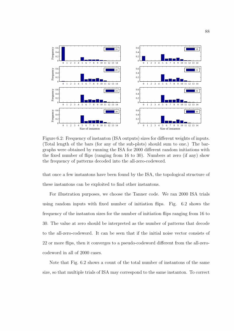
88
0 1 2 3 4 5 6 7 8 9 10 11 12 13 140
0.2
0.4
0.6
Fre
quen
cy
16
0 1 2 3 4 5 6 7 8 9 10 11 12 13 140
0.2
0.4
0.6
18
0 1 2 3 4 5 6 7 8 9 10 11 12 13 140
0.2
0.4
0.6
Fre
quen
cy
20
0 1 2 3 4 5 6 7 8 9 10 11 12 13 140
0.2
0.4
0.6
22
0 1 2 3 4 5 6 7 8 9 10 11 12 13 140
0.2
0.4
0.6
Fre
quen
cy
24
0 1 2 3 4 5 6 7 8 9 10 11 12 13 140
0.2
0.4
0.6
26
0 1 2 3 4 5 6 7 8 9 10 11 12 13 140
0.2
0.4
0.6
Size of instanton
Fre
quen
cy
28
0 1 2 3 4 5 6 7 8 9 10 11 12 13 140
0.2
0.4
0.6
Size of instanton
30
Figure 6.2: Frequency of instanton (ISA outputs) sizes for different weights of inputs.(Total length of the bars (for any of the sub-plots) should sum to one.) The bar-graphs were obtained by running the ISA for 2000 different random initiations withthe fixed number of flips (ranging from 16 to 30). Numbers at zero (if any) showthe frequency of patterns decoded into the all-zero-codeword.
that once a few instantons have been found by the ISA, the topological structure of
these instantons can be exploited to find other instantons.
For illustration purposes, we choose the Tanner code. We ran 2000 ISA trials
using random inputs with fixed number of initiation flips. Fig. 6.2 shows the
frequency of the instanton sizes for the number of initiation flips ranging from 16 to
30. The value at zero should be interpreted as the number of patterns that decode
to the all-zero-codeword. It can be seen that if the initial noise vector consists of
22 or more flips, then it converges to a pseudo-codeword different from the all-zero-
codeword in all of 2000 cases.
Note that Fig. 6.2 shows a count of the total number of instantons of the same
size, so that multiple trials of ISA may correspond to the same instanton. To correct

89
for this multiplicity in counting, one can also find it useful (see discussions below) to
study the total number of unique instantons observed in the ISA trials, coined the
Instanton-Bar-Graph. Fig. 6.3 shows the number of distinct instantons of a given
size for 2000 and 5000 random initiations with 20 flips. One finds that the total
number of ISA outputs of size 5 after 2000 trails is 720, however representing only
155 distinct instantons. In this case (of the Tanner code), we can independently
verify 1 that the total number of instantons of size 5 is indeed 155, thus confirming
that our algorithm has found all the instantons of length 5 detecting each of them
roughly 4 times. Obviously, the total number of distinct instantons of size 5 does not
change with further increase in the number of trails. This observation emphasizes
utility of the sub-plots, with different number of initiations, as the comparison allows
to judge the sufficiency (or insufficiency) of the number of trials for finding all the
given size instantons. Extending the comparison to larger size (> 5) instantons,
one observes that the numbers change in transition from 2000 to 5000 trials, thus
indicating that the statistics is insufficient (at least after 2000 trials) as some of the
instantons have not been found yet. The smallest weight instanton found by the
ISA is 5 thereby indicating that the slope of the FER curve in the error floor region
is five.
6.3 Code Construction Avoiding Certain Topological Structures
The minimum pseudo-codeword weight (as well as the trapping set size) increase
with increase of the Tanner graph girth (see [41, 52]). While girth optimized codes
1We have observed that all the instantons of size 5 are in fact the (5, 3) trapping sets described
in [54]. Further investigation of the topological structure of instantons will be dealt in future work.

90
1 2 3 4 5 6 7 8 9 10 11 12 13 140
100
200
300
400
500
600
700
Size of instanton
Num
ber
of u
niqu
e in
stan
tons
20005000
Figure 6.3: Instanton-Bar-Graph showing the number of unique instantons of a givenweight found by running the ISA with 20 random flips for 2000 and 5000 initiationsrespectively.
are known to perform better in general, the code length and degree distribution
place a fundamental restriction on the best achievable girth. Observing that the
instantons for different decoding algorithms performing over different channels have
a common underlying topological structure (e.g. the (5, 3) trapping set in the case
of the Tanner code), it is natural to discuss design of a similar but new code which
excludes these troublesome structures. In fact, this suggests a natural code opti-
mization technique with an improved instanton distribution. Starting with a reason-
ably good code (constructed either algebraically or by the progressive edge growth
(PEG) method [66]), we find the most damaging instantons and their underlying
topological structure. We then construct a new code avoiding such subgraphs (either
by swapping edges, by increasing code length, or utilizing a combination of both).
We iterate this procedure till the code can no longer be optimized or we reach a

91
computationally unbearable complexity.
For Gallager A decoding, it has been proved in [56] that codes with Tanner
graphs of girth 8 which avoid the (5, 3) trapping set and weight 8 codewords can
correct all the error patterns of weight 3 or less. While proving a similar result
might be difficult for the iterative decoder over the AWGN channel and LP decoder,
such considerations nonetheless play a role in our code design strategy. An algo-
rithm, suggesting construction of a code meeting the Gallager A-related conditions,
was provided in [56]. This algorithm can be seen as a generalization of the PEG
algorithm [66]. Given a list of forbidden subgraphs, at every step of the algorithm,
an edge is established such that the resulting graph at that stage does not consist
of any of the forbidden subgraphs. (The PEG algorithm is a special case forbidding
cycles shorter than a given threshold.)
Using the algorithm proposed in [56], we constructed a new code of length 155
with uniform left degree 3 and with most check nodes with degree 5. By construction,
this code avoids (5, 3) trapping sets. This results in a steeper FER slope of 4 in
the error floor domain under the Gallager A decoder, as shown in Fig. 6.4. The
minimum weight instanton for LP decoder over the BSC found by the ISA is 6. Fig.
6.4 shows FER performance of the Tanner code and the new code under Gallager A
and LP decoders. The instanton distribution for LP decoding over the BSC for the
Tanner code and the new code found by running the ISA for 2000 times is shown in
Fig. 6.5. All the above statistics illustrate the superiority of the new code.
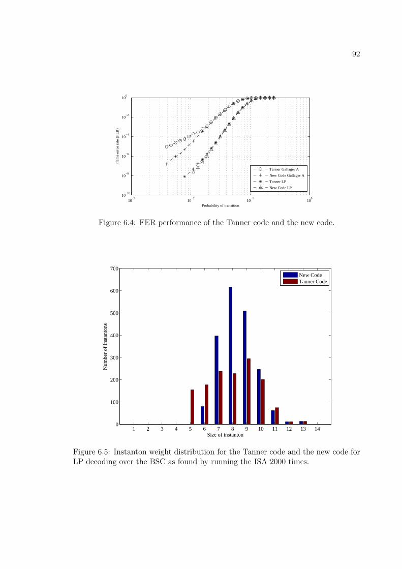
92
10−3
10−2
10−1
100
10−10
10−8
10−6
10−4
10−2
100
Probability of transition
Fra
me
erro
r ra
te (
FE
R)
Tanner Gallager A
New Code Gallager A
Tanner LP
New Code LP
Figure 6.4: FER performance of the Tanner code and the new code.
1 2 3 4 5 6 7 8 9 10 11 12 13 140
100
200
300
400
500
600
700
Size of instanton
Num
ber
of in
stan
tons
New CodeTanner Code
Figure 6.5: Instanton weight distribution for the Tanner code and the new code forLP decoding over the BSC as found by running the ISA 2000 times.

93
CHAPTER 7
Concluding Remarks
I do not know what I may appear to the world, but to myself I seem to
have been only like a boy playing on the sea-shore, and diverting myself in
now and then finding a smoother pebble or a prettier shell than ordinary,
whilst the great ocean of truth lay all undiscovered before me.
Sir Isaac Newton
We have investigated the problem of guaranteed error correction capability of LDPC
codes under various hard decision decoding algorithms. The results presented in
this work are only a first step toward understanding the decoding failures of various
decoders for finite length LDPC codes. One readily identifies that the discussion in
the preceding chapters was limited to regular binary LDPC codes and specific hard
decision decoding algorithms. We can identify a large class of problems that arise
as direct or indirect consequences of the results reported in this dissertation. We
list below a few ongoing investigations and also indicate possible future directions
for research.
• Extension to irregular codes: Trapping set/ pseudo-codeword analysis for
ensembles of irregular codes is an important theoretical problem as it is gen-
erally known that irregular degree distributions achieve capacity on a variety
of channels [18].

94
• Extension to soft decision decoding algorithms: Hard decision algo-
rithms are convenient from an analysis point of view but most of the practical
systems employ soft decision algorithms. Analysis of multi-bit decoders is a
first step in this process.
• Analysis of classes of codes: A wide variety of structured codes have
been investigated for practical implementations. An important class of such
codes is the protograph-based codes [67]. Trapping set/pseudo-codeword
analysis for such codes allows construction of codes with low-complexity en-
coders/decoders.
• Extension to non-binary LDPC codes: Many properties of non-binary
LDPC codes [11] are largely unknown owing to the complexity of the decoding
algorithms. Study of simple hard decision algorithms and their asymptotic
analysis are one of the many interesting problems in this area.
• Practical LP Decoders: While very attractive from a theoretical point of
view, LP decoders suffer from huge computational complexity. Methods that
successively improve LP decoding by adding constraints hold lot of promise
for implementation purposes. The interested reader is referred to [68, 69, 70,
71, 72] for introduction to these problems.
• Extension to GLDPC codes: Generalized LDPC (GLDPC) codes [12] have
many interesting properties and it would be interesting to see how their error
correction capability depends on column weight and error correction capability
of the sub-code (see [53] for initial results).
While the above mentioned problems are important from a theoretical stand-

95
point, it should be kept in mind that the ultimate purpose of the analysis methods
developed and presented in this work is to aid in the construction of codes with
good error floor performance. To this end, it is of utmost importance to formulate
better and tighter bounds for higher column weight codes and derive necessary and
sufficient conditions to guarantee correction of certain number of errors. Answers to
the above questions will help in system architectures that guarantee superior error
floor performance.

96
APPENDIX A
Column-Weight-Three Codes with Tanner Graphs of Girth Less Than
10
In Chapter 3, we established a relation between the size of inducing set and the girth
of Tanner graph for a column-weight-three LDPC code. The results of Chapter 3 and
Chapter 4, provide unambiguous bounds on minimum number of errors correctable
by the Gallager A algorithm for codes with Tanner graphs of girth greater than
eight. However, there still remains some ambiguity about codes with girth less than
or equal to eight.
We have shown in Lemma 3.3, that a code with girth g = 4 always has an
inducing set of size two or three. It is unlikely for a code with girth g = 4 not
to contain an inducing set of size two and even if such a code exists it might be
very difficult to construct such a code. So, it is safe to assume that a code with
Tanner graph of girth g = 4 cannot correct two errors. We are now tempted to ask
under what conditions can it correct a single error. It can easily be seen that this
is possible if the Tanner graph does not contain codewords of weight two, a result
that is hardly surprising. Similarly, it can be said that a code with Tanner graph
of girth g = 6 cannot correct three errors and can correct two errors if the Tanner
graph avoids codewords of weight four. We will not elaborate on these results as it
is easy to consider all possible configurations and derive the conditions.
The problem of correction of three errors is relatively more complicated. As we
have observed that codes with Tanner graph of girth g = 6 cannot correct three

97
errors (with high probability), we conclude that the girth should be at least eight.
However, girth of eight alone cannot guarantee correction of three errors as there
can be trapping sets that have critical number three. In this chapter, we prove
that apart from the (3, 3) trapping sets, there exist two more trapping sets, namely
(5, 3) trapping set and (8, 0) trapping set that can have critical number three. We
also show that avoiding structures isomorphic to these trapping sets guarantees
correction of three errors.
A.1 The Case of Codes with Tanner Graphs of Girth Eight
Lemma A.1. There exist (5,3) and (8,0) trapping sets with critical number three
and no (5,3) or (8,0) trapping sets with critical number less than three.
Proof. We prove the lemma for the case of (5, 3) trapping sets and omit the proof
for (8, 0) trapping sets. Consider the (5, 3) trapping set shown in Fig. A.1. Let
V 1 := {v11, v
12, v
13} be the set of variables which are initially in error. Let C1 :=
{c11, c
12, . . . , c
19} and V 2 := {v2
1, v22}. Also, assume that no variable node in V \(V 1 ∪
V 2), has two or more neighbors in C1. In the first iteration, we have:
ω1(v, c) =
1 if v ∈ V 1
0 otherwise(A.1)
ω1(c, v) =
1 if c ∈ C1, v /∈ V 1
0 otherwise(A.2)
Consequently, all variable nodes in V 2 are decoded incorrectly at the end of the first

98
(a) (b)
(c) (d)
Figure A.1: Illustration of message passing for a (5, 3) trapping set: (a) variableto check messages in round one; (b) check to variable messages in round one; (c)variable to check messages in round two; and (d) check to variable messages in roundtwo. Arrow-heads indicate the messages with value 1.
iteration. In the second iteration:
ω2(v, c) =
1 if v ∈ V 2
0 otherwise(A.3)
ω2(c, v) =
1 if c ∈ C1\{c12, c
15, c
18}, v /∈ V 2
0 otherwise(A.4)
and all variable nodes in V 1 are decoded incorrectly. Continuing in this fashion,
ω3(v, c) = ω1(v, c) and ω3(c, v) = ω1(c, v). That is, the messages being passed in the
Tanner graph would repeat after every two iterations. Hence, three variable nodes
in error initially can lead to a decoder failure and therefore, this (5, 3) trapping set
has critical number equal to three.
Theorem A.2. To guarantee that three errors in a column-weight-three LDPC code
can be corrected by the Gallager-A algorithm, it is necessary to avoid (3, 3), (5, 3)
and (8, 0) trapping sets in its Tanner graph.

99
(a) (b) (c)
(d) (e)
Figure A.2: All the possible subgraphs that can be induced by three variable nodesin a column-weight-three code
Proof. Follows from the discussion above.
We now state and prove the main theorem.
Theorem A.3. If the Tanner graph of a column-weight-three LDPC codes has girth
eight and does not contain a subgraph isomorphic to a (5, 3) trapping set or a sub-
graph isomorphic to an (8, 0) trapping set, then any three errors can be corrected
using the Gallager-A algorithm.
Proof. Let V 1 := {v11, v
12, v
13} be the three erroneous variables and C1 be the set of
the checks connected to the variables in V 1. In a column-weight-three code (free of
cycles of length four) the variables in V 1 can induce only one of the five subgraphs
given in Fig. A.2. In each case, ω1(v, :) = {1} if v ∈ V 1 and is 0 otherwise. The proof
proceeds by examining these subgraphs one at a time and proving the correction of
the three erroneous variables in each case.
Subgraph 1: Since the girth of the code is eight, it has no six cycles. Hence,
the configuration in Fig. A.2(a) is not possible.
Subgraph 2: The variables in V 1 induce the subgraph shown in Fig. A.2(b).

100
At the end of the first iteration:
ω1(c, v) =
1 if c ∈ C1, v /∈ V 1
0 otherwise(A.5)
There cannot exist a variable node which is connected to two or more checks in
the set C1 without introducing either a six-cycle or a subgraph isomorphic to (5, 3)
trapping set. At the end of first iteration, ω1(:, v) = {0} for all v ∈ V 1. Furthermore,
there exists no v /∈ V 1 for which ω1(:, v) = {1}. Hence, if a decision is made after
the first iteration, a valid codeword is found and the decoder is successful.
Subgraph 3: The variables in V 1 induce the subgraph shown in Fig. A.2(c).
At the end of the first iteration:
ω1(c, v) =
1 if c ∈ C1\{c13, c
15}, v /∈ V 1
1 if c ∈ {c13, c
15}, v ∈ V 1
0 otherwise
(A.6)
For no v /∈ V 1, ω1(:, v) = {1} as this would introduce a four-cycle or a six-cycle in
the graph. For any v /∈ V 1, ω2(v, c) = 1 only if ω1(: \c, v) = {1}. This implies that
v has two checks in C1\{c13, c
15}. Let V 2 be the set of such variables. We have the
following lemma:
Lemma A.4. There can be at most one variable in V 2.
Proof. Suppose |V 2| = 2. Specifically, assume V 2 = {v21, v
22}. The proof is similar
for |V 2| > 2. First note that for any v ∈ V 2, v cannot be connected to c14 as it would
create a six-cycle. Next, let C11 := {c1
1, c12} and C1
2 := {c16, c
17}. Then, v cannot
have both checks in either C11 or C1
2 as this would cause a four-cycle. Hence, v has
one check in C11 and one check in C1
2 . Assume without loss of generality that v21 is

101
connected to c11 and c1
6. Then, v22 cannot be connected to c1
1 and c17 as this would
form a six-cycle. v22 cannot be connected to c1
2 and c17 as it would create a (5, 3)
trapping set. Hence, |V 2| < 2.
Let v21 ∈ V 2 be connected to c1
1, c16 and an additional check c2
1. In the second
iteration:
ω2(v, c) =
1 if v ∈ {v11, v
13}, c /∈ {c1
3, c15}
1 if v = v12
1 if v = v21, c = c2
1
0 otherwise
(A.7)
ω2(c, v) =
1 if c ∈ C1\{c14}, v /∈ V 1
1 if c ∈ {c13, c
14, c
15}, v 6= v1
2
1 if c = c21, v 6= v2
1
0 otherwise
(A.8)
We have the following lemma:
Lemma A.5. There cannot exist any variable v /∈ V 1⋃
V 2 such that it receives two
or more incorrect messages at the end of the second iteration.
Proof. Suppose there existed a variable v such that it received two incorrect mes-
sages in the second iteration. Then, it would be connected to two checks in the
set C1⋃
{c21}. This is not possible as it would introduce a four-cycle, six-cycle or a
(5, 3) trapping set (e.g. if v is connected to c14 and c2
1, it would form a (5, 3) trapping
set).

102
Thus, in the third iteration:
ω3(v, c) =
1 if v ∈ {v11, v
13}, c /∈ {c1
3, c15}
1 if v = v21, c = c2
1
0 otherwise
(A.9)
ω3(c, v) =
1 if c ∈ {c11, c
12, c
16, c
17}, v /∈ {v1
1, v13}
1 if c = c21, v 6= v2
1
0 otherwise
(A.10)
At the end of the third iteration, ω3(:, v) = {0} for all v ∈ V 1. Also, we have the
following lemma:
Lemma A.6. There exists no v /∈ V 1 such that ω3(:, v) = {1}.
Proof. Suppose there exists v such that ω3(:, v) = {1}. Then, v is connected to
three checks in the set {c11, c
12, c
16, c
17, c
21}. This implies that ω2(:, v) = {1}. However,
from Lemma A.5 it is evident that no such v exists.
Hence, if a decision is made after the third iteration, a valid codeword is found
and the decoder is successful.
Subgraph 4: The variables in V 1 induce the subgraph shown in Fig. A.2(d).
At the end of the first iteration:
ω1(c, v) =
1 if c ∈ C1\{c13}, v /∈ V 1
1 if c = c13, v ∈ {v1
1, v12}
0 otherwise
(A.11)
For no v ∈ V \V 1, ω2(:, v) = {1}. For any v ∈ V \V 1, ω2(v, c) = 1 only if ω1(:
\c, v) = {1}. Let V 2 be the set of all such variables. We have the following lemma:

103
Lemma A.7. (i) V 2 has at most four variables, and (ii) No two variables in V 2
can share a check in C\C1.
Sketch of the Proof : There exists no variable which is connected to two checks
from the set {c11, c
12, c
13, c
14, c
15} as it would introduce a four-cycle or a six-cycle. How-
ever, a variable node can be connected to one check from {c11, c
12, c
13, c
14, c
15} and to
one check from {c16, c
17, c
18}. There can be at most four such variable nodes. When
four such variable nodes exist, none are connected to c13. Also, these four variable
nodes cannot share checks outside the set C1\{c13}.
Let these four variable nodes be labeled v21, v2
2, v23 and v2
4 and their third checks c21,
c22, c2
3 and c24, respectively. Let C2 := {c2
1, c22, c
23, c
24}. Hence, in the second iteration:
ω2(v, c) =
1 if v ∈ {v11, v
12}, c 6= c1
3
1 if v ∈ V 2, c ∈ C2
0 otherwise
(A.12)
ω2(c, v) =
1 if c ∈ {c11, c
12, c
14, c
15}, v /∈ {v1
1, v12}
1 if c ∈ C2, v /∈ V 2
0 otherwise
(A.13)
At the end of the second iteration ω2(:, v) = {0} for all v ∈ V 1. Moreover, for no
v /∈ V 1, ω2(:, v) = {1}. So, if a decision is made after the second iteration, a valid
codeword is reached and the decoder is successful.
Subgraph 5: The variables in V 1 induce the subgraph shown in Fig. A.2(e).
At the end of the first iteration:
ω1(c, v) =
1 if c ∈ C1, v /∈ V 1
0 otherwise(A.14)

104
If there exists no variable v ∈ V \V 1 such that ω1(:, v) = {1}, a valid codeword is
reached after the first iteration. Suppose this is not the case. Let V 2 be the set of
variables which receive two or more incorrect messages. Then, we have the following
lemma:
Lemma A.8. (i) There exists one variable v21 ∈ V 2 such that ω1(:, v
21) = {1}, and
(ii) V 2 has at most three variables which receive two incorrect messages at the end
of the first iteration. Furthermore, they cannot share a check in C\C1.
Proof. We omit the proof of Part (ii) as it is straightforward. Part (i) is proved
as follows: If there existed no variable, v21, such that ω1(:, v
21) = {1}, then the
decoder would converge in one iteration. Next, suppose v21, v
22 ∈ V 2 such that
ω1(:, v21) = ω1(:, v
22) = {1}. Without loss of generality, let v2
1 be connected to c11, c
14
and c17. Then, v2
1 would share two checks in the set C1. It is then not possible
to connect v22 without introducing a six-cycle or a (5, 3) trapping set (e.g., if v2
1 is
connected to c12, c1
5 and c18, then it would introduce a (5, 3) trapping set).
Let the third checks connected to v22, v2
3 and v24 be c2
1, c22 and c2
3, respectively and
let C2 := {c21, c
22, c
23} In the second iteration:
ω2(v, c) =
1 if v = v21
1 if v ∈ V 2\{v21}, c ∈ C2
0 otherwise
(A.15)
ω2(c, v) =
1 if c ∈ {c11, c
13, c
17}, v 6= v2
1
1 if c ∈ C2, v /∈ V 2
0 otherwise
(A.16)
There cannot exist a variable node which is connected to one check from C2 and to

105
one check from {v11, v
14, v
17}. Also, there cannot be a variable node which is connected
to all three checks in the set C2 as this would introduce a graph isomorphic to
the (8, 0) trapping set. However, there can be at most two variable nodes which
receive two incorrect messages from the checks in C2, say v31 and v3
2. Let the third
checks connected to them be c31 and c3
2, respectively. Let V 3 := {v31, v
32} and C3 :=
{c31, c
32}. At the end of the second iteration, variables v1
1, v12 and v1
3 receive one
incorrect message each. Variables in the set V 3 receive two incorrect messages each.
Therefore, in the third iteration, we have:
ω3(v, c) =
1 if v ∈ V 1, c /∈ {c11, c
14, c
17}
1 if v ∈ V 3, c ∈ C3
0 otherwise
(A.17)
ω3(c, v) =
1 if c ∈ C1\{c11, c
14, c
17}, v /∈ V 1
1 if c ∈ C3, v /∈ V 3
(A.18)
At the end of the third iteration, ω3(:, v) = {1} for all v ∈ V 1. Furthermore, for
no v /∈ V 1, ω3(:, v) = 1. So, if a decision is made after the third iteration, a valid
codeword is reached and the decoder is successful.

106
APPENDIX B
Finding Instantons for LP Decoding Over the BSC
The pseudo-codewords and instantons for LP decoding cannot entirely be deter-
mined from combinatorial considerations. Hence, we adopt an algorithmic approach
to identify and enumerate instantons for LP decoding over the BSC.
Definition B.1. The median noise vector (or simply the median) M(p) of a pseudo-
codeword p distinct from the all-zero-codeword is a binary vector with support
S = {v1, v2, . . . , vq}, such that pv1, . . . , pvq
are the q(= ⌈(wBSC(p) + 1) /2⌉) largest
components of p.
One observers that, C (M(p),p) ≤ 0. From the definition of wBSC(p), it fol-
lows that at least one median exists for every p. Also, all medians of p have
⌈(wBSC(p) + 1) /2⌉ flips. The proofs of the following two lemmas are now apparent.
Lemma B.2. The LP decoder decodes a binary vector with q flips into a pseudo-
codeword p distinct from the all-zero-codeword iff wBSC(p) ≤ 2q.
Lemma B.3. Let p be a pseudo-codeword with median M(p) whose support has
cardinality q. Then wBSC(p) ∈ {2q − 1, 2q}.
Lemma B.4. Let M(p) be a median of p with support S. Then the result of LP
decoding of any binary vector with support S ′ ⊂ S and |S ′| < |S| is distinct from p.
Proof. Let |S| = q. Then by Lemma B.3, wBSC(p) ∈ {2q − 1, 2q}. Now, if r is any
binary vector with support S ′ ⊂ S, then r has at most q − 1 flips and therefore by
Lemma B.2, wBSC(p) ≤ 2(q − 1), which is a contradiction.
107
Lemma B.5. If M(p) converges to a pseudo-codeword pM 6= p, then wBSC(pM) ≤
wBSC(p). Also, C(M(p),pM) ≤ C(M(p),p).
Proof. According to the definition of the LP decoder, C(M(p),pM) ≤ C(M(p),p).
If wBSC(p) = 2q, then M(p) has q flips and by Lemma B.2, wBSC(pM) ≤ 2q =
wBSC(p).
If wBSC(p) = 2q − 1, then M(p) has q flips and C(M(p),p) < 0. Hence,
wBSC(pM) ≤ 2q by Lemma B.2. However, if wBSC(pM) = 2q, then C(M(p),pM) =
0, which is a contradiction. Hence, wBSC(pM) ≤ 2q − 1 = wBSC(p).
The following lemma follows from the definition of the cost of decoding (the
pseudo-codeword cost):
Lemma B.6. Let i be an instanton. Then for any binary vector r such that
supp(i) ⊂ supp(r), there exists a pseudo-codeword p satisfying C(r,p) ≤ 0.
Proof. Since i is an instanton, there exists a pseudo-codeword p such that C(i,p) ≤
0. From Definition 2.13 we have,
∑
v/∈supp(i)
pv −∑
v∈supp(i)
pv ≤ 0.
Since, supp(i) ⊂ supp(r) and pv ≥ 0,∀v, we have
∑
v/∈supp(r)
pv −∑
v∈supp(r)
pv ≤ 0,
thus yielding
C(r,p) ≤ 0.

108
The above lemma implies that the LP decoder fails to decode every vector r
whose support is a superset of an instanton to the all-zero- codeword. We now have
the following corollary:
Corollary B.7. Let r be a binary vector with support S. Let p be a pseudo-codeword
such that C(r,p) ≤ 0. If all binary vectors with support S ′ ⊂ S such that |S ′| =
|S| − 1, converge to 0, then r is an instanton.
The above lemmas lead us to the following lemma which characterizes all the
failures of the LP decoder over the BSC:
Lemma B.8. A binary vector r converges to a pseudo-codeword different from the
all-zero-codeword iff the support of the vector r contains the support of an instanton
as a subset.
The most general form of the above lemma can be stated as following: if x is the
transmitted codeword and y is the received vector, then y converges to a pseudo-
codeword different from x iff the supp(y + x), where the addition is modulo two,
contains the support of an instanton as a subset.
From the above discussion, we see that the BSC instantons are analogous to the
minimal stopping sets for the case of iterative/LP decoding over the BEC. In fact,
Lemma B.8 characterizes all the decoding failures of the LP decoder over the BSC
in terms of the instantons and can be used to derive analytical estimates of the
code performance given the weight distribution of the instantons. In this sense, the
instantons are more fundamental than the minimal pseudo-codewords [43, 41] for
the BSC (note, that this statement does not hold in the case of the AWGN channel).
Two minimal pseudo-codewords of the same weight can give rise to different number
109
of instantons. This issue was first pointed out by Forney et al. in [35]. (See Examples
1, 2, 3 for the BSC case in [35].) It is also worth noting that an instanton converges
to a minimal pseudo-codeword.
It should be noted that finding pseudo-codewords with fractional weight dfrac
is not equivalent to finding minimum weight pseudo-codewords. The pseudo-
codewords with fractional weight dfrac can be used to derive some instantons, but
not necessarily the ones with the least number of flips. However, as dfrac provides
a lower bound on the minimum pseudo-codeword weight, it can be used as a test if
the ISA actually finds an instanton with the least number of flips. In other words,
if the number of flips in the lowest weight instanton found by the ISA is equal to
⌈dfrac/2⌉, then the ISA has indeed found the smallest size instanton.
B.1 Instanton Search Algorithm and its Analysis
In this Section, we describe the Instanton Search Algorithm. The algorithm starts
with a random binary vector with some number of flips and outputs an instanton.
Instanton Search Algorithm
Initialization (j=0) step: Initialize to a binary input vector r containing sufficient
number of flips so that the LP decoder decodes it into a pseudo-codeword different
from the all-zero-codeword. Apply the LP decoder to r and denote the pseudo-
codeword output of LP by p1.
j ≥ 1 step: Take the pseudo-codeword pj (output of the (j − 1) step) and calculate
its median M(pj). Apply the LP decoder to M(pj) and denote the output by pMj.
By Lemma B.5, only two cases arise:
• wBSC(pMj) < wBSC(pj). Then pj+1 = pMj
becomes the j-th step output/(j +

110
(a) (b) (c)
(d)
0
(e)
Figure B.1: Squares represent pseudo-codewords and circles represent medians or re-lated noise configurations (a) LP decodes median of a pseudo-codeword into anotherpseudo-codeword of smaller weight (b) LP decodes median of a pseudo-codeword intoanother pseudo-codeword of the same weight (c) LP decodes median of a pseudo-codeword into the same pseudo-codeword (d) Reduced subset (three different greencircles) of a noise configuration (e.g. of a median from the previous step of theISA) is decoded by the LP decoder into three different pseudo-codewords (e) LP de-codes the median (blue circle) of a pseudo-codeword (low red square) into anotherpseudo-codeword of the same weight (upper red square). Reduced subset of themedian (three configurations depicted as green circles are all decoded by LP intoall-zero-codeword. Thus, the median is an instanton.
1) step input.
• wBSC(pMj) = wBSC(pj). Let the support of M(pj) be S = {i1, . . . , ikj
}.
Let Sit = S\{it} for some it ∈ S. Let rit be a binary vector with support Sit .
Apply the LP decoder to all rit and denote the it-output by pit . If pit = 0,∀it,
then M(pj) is the desired instanton and the algorithm halts. Else, pit 6= 0
becomes the j-th step output/(j + 1) step input. (Notice, that Lemma B.4
guarantees that any pit 6= pj, thus preventing the ISA from entering into an
infinite loop.)
Fig. B.1 illustrates different scenarios arising in the execution of the ISA.
Here, the squares represent pseudo-codewords and the circles represent binary vec-

111
tors (noise configurations). Two squares of the same color have identical pseudo-
codeword weight and two circles of the same color consist of same number of flips.
Fig. B.1(a) shows the case where a median, M(pl), of a pseudo-codeword pj con-
verges to a pseudo-codeword pMjof a smaller weight. In this case, pj+1 = pMj
. Fig.
B.1(b) illustrates the case where a median, M(pj), of a pseudo-codeword pj con-
verges to a pseudo-codeword pMjof the same weight. Fig. B.1(c) illustrates the case
where a median, M(pj), of a pseudo-codeword pj converges to the pseudo-codeword
pj itself. In the two latter cases, we consider all the binary vectors whose support
sets are subsets of the support set of M(pj) and the vectors contain one flip less. We
run the LP decoder with the vectors as inputs and find their corresponding pseudo-
codewords. One of the non-zero pseudo-codewords found is chosen at random as
pj+1. This is illustrated in Fig. B.1(d). Fig. B.1(e) shows the case when all the
subsets of M(pj) (reduced by one flip) converge to the all-zero-codeword. M(pj)
itself could converge to pj or some other pseudo-codeword of the same weight. In
this case, M(pj) is an instanton constituting the output of the algorithm.
We now prove that the ISA terminates (i.e., outputs an instanton) in the number
of steps of the order the number of flips in the initial noise configuration.
Theorem B.9. wBSC(pj) and |supp(M(pj))| are monotonically decreasing. Also,
the ISA terminates in at most 2k0 steps, where k0 is the number of flips in the input.
Proof. If pj+1 = pMj, then wBSC(pj+1) < wBSC(pj). Consequently,
|supp(M(pj+1))| ≤ |supp(M(pj))|.
If pj+1 = pit , then wBSC(pit) ≤ 2(|supp(M(pj))| − 1) < wBSC(pj). Conse-
quently, |supp(M(pj+1))| ≤ |supp(M(pj))|.
Since wBSC(pj) is strictly decreasing, the weight of pseudo-codeword at step j

112
decreases by at least one compared to the weight of the pseudo-codeword at step
j − 1. Since by Lemma B.2, wBSC(p1) ≤ 2k0, the algorithm can run for at most 2k0
steps.
Remarks: (1) By “sufficient number of flips”, we mean that the initial binary
vector should be noisy enough to converge to a pseudo-codeword other than the
all-zero-codeword. While any binary vector with a large number of flips is almost
guaranteed to converge to a pseudo-codeword different from the all-zero-codeword,
such a choice might also lead to a longer running time of the ISA (from Theorem
B.9). On the other hand, choosing a binary vector with a few number of flips might
lead to convergence to the all-zero-codeword very often, thereby necessitating the
need to run the ISA for a large number of times.
(2) Theorem B.9 does not claim that the algorithm finds the minimum weight
pseudo-codeword or the instanton with the smallest number of flips. However, it is
sometimes possible to verify if the algorithm has found the minimum weight pseudo-
codeword. Let wISAmin denote the weight of the minimum weight pseudo-codeword
found by the ISA. If wISAmin = 2⌈dfrac/2⌉ − 1, then wISA
min = wBSCmin .
(3) At some step j, it is possible to have wBSC(pMj) = wBSC(pj) and incorpo-
rating such pseudo-codewords into the algorithm could lead to lower weight pseudo-
codewords in the next few steps. However, this inessential modification was not
included in the ISA to streamline the analysis of the algorithm.
(4) While we have shown that wBSC(pj) decreases by at least unity at every step,
we have observed that in most cases, it decreases by at least two. This is due to
the fact that the pseudo-codewords with odd weights outnumber pseudo-codewords
with even weights. As a result, in most cases, the algorithm converges in less than
113
k0 steps. (For illustration of this point see example discussed in the next Section.)
(5) At any step, there can be more than one median, and the ISA does not
specify which one to pick. Our current implementation suggests to pick a median
at random. Also, the algorithm does not provide clarification on the choice of
the pseudo-codeword for the case when more than one noise configurations from
the subset rit converge to pseudo-codewords distinct from the all-zero-codeword.
In this degenerate case, we again choose a pseudo-codeword for the next iteration
at random. Note that one natural deterministic generalization of the randomized
algorithm consists of exploring all the possibilities at once. In such a scenario, a
tree of solutions can be built, where the root is associated with one set of initiation
flips, any branch of the tree relates to a given set of randomized choices (of medians
and pseudo-codewords), and any leaf corresponds to an instanton.
114
REFERENCES
[1] C. E. Shannon, “A mathematical theory of communication,” Bell system tech-
nical journal, vol. 27, 1948.
[2] R. W. Hamming, “Error detecting and error correcting codes.” Bell Syst. Tech.
Jrnl., vol. 29, pp. 147–160, 1950.
[3] A. Hocquenghem, “Codes correcteurs d’erreurs,” Chiffres (Paris), vol. 2, pp.
147–156, September 1959.
[4] R. C. Bose and D. K. Ray-Chaudhuri, “On a class of error correcting binary
group codes,” Information and Control, vol. 3, no. 1, pp. 68–79, March 1960.
[5] I. S. Reed and G. Solomon, “Polynomial codes over certain finite fields,” Jour-
nal of the Society for Industrial and Applied Mathematics, vol. 8, no. 2, pp.
300–304, 1960.
[6] S. Lin and Costello, Error Control Coding: Fundamentals and Applications.
Englewood Cliffs, NJ: Prentice-Hall, 1983.
[7] M. Sudan, “Decoding of Reed-Solomon codes beyond the error-correction
bound,” Journal of Complexity, vol. 13, pp. 180–193, 1997.
[8] R. Koetter and A. Vardy, “Algebraic soft-decision decoding of Reed-Solomon
codes,” Information Theory, IEEE Transactions on, vol. 49, no. 11, pp.
2809–2825, 2003. [Online]. Available: http://ieeexplore.ieee.org/xpls/
abs\ all.jsp?arnumber=1246007
115
[9] A. Viterbi, “Error bounds for convolutional codes and an asymptotically
optimum decoding algorithm,” Information Theory, IEEE Transactions
on, vol. 13, no. 2, pp. 260–269, 1967. [Online]. Available: http:
//ieeexplore.ieee.org/xpls/abs\ all.jsp?arnumber=1054010
[10] C. Berrou, A. Glavieux, and P. Thitimajshima, “Near Shannon limit error-
correcting coding and decoding: Turbo codes,” in Proc. IEEE Int. Conf. on
Communications, vol. 2, 1993, pp. 1064–1070.
[11] R. G. Gallager, Low Density Parity Check Codes. Cambridge, MA: M.I.T.
Press, 1963.
[12] R. M. Tanner, “A recursive approach to low complexity codes,” IEEE Trans.
Inform. Theory, vol. 27, no. 5, pp. 533–547, 1981.
[13] D. J. C. Mackay, “Good error-correcting codes based on very sparse matrices,”
IEEE Trans. Inform. Theory, vol. 45, no. 2, pp. 399–431, 1999.
[14] F. R. Kschischang, B. J. Frey, and H. A. Loeliger, “Factor graphs and the sum-
product algorithm,” IEEE Trans. Inform. Theory, vol. 47, no. 2, pp. 498–519,
2001.
[15] J. Pearl, Probablisitic Reasoning in Intelligent Systems. San Francisco, CA:
Kaufmann, 1988.
[16] V. V. Zyablov and M. S. Pinsker, “Estimation of the error-correction complexity
for Gallager low-density codes,” Problems of Information Transmission, vol. 11,
no. 1, pp. 18–28, 1976.

116
[17] T. J. Richardson and R. Urbanke, “The capacity of low-density parity-check
codes under message-passing decoding,” IEEE Trans. Inform. Theory, vol. 47,
no. 2, pp. 599–618, 2001.
[18] T. J. Richardson, M. Shokrollahi, and R. Urbanke, “Design of capacity-
approaching irregular low-density parity-check codes,” IEEE Trans. Inform.
Theory, vol. 47, no. 2, pp. 638–656, 2001.
[19] L. Bazzi, T. Richardson, and R. Urbanke, “Exact thresholds and optimal codes
for the binary symmetric channel and Gallager’s decoding algorithm A,” IEEE
Trans. Inform. Theory, vol. 50, pp. 2010–2021, 2004.
[20] M. Sipser and D. Spielman, “Expander codes,” IEEE Trans. Inform. Theory,
vol. 42, no. 6, pp. 1710–1722, 1996.
[21] A. Barg and G. Zemor, “Error exponents of expander codes,” IEEE Trans.
Inform. Theory, vol. 48, no. 6, pp. 1725–1729, 2002.
[22] D. Burshtein and G. Miller, “Expander graph arguments for message-passing
algorithms,” IEEE Trans. Inform. Theory, vol. 47, no. 2, pp. 782–790, 2001.
[23] D. Burshtein, “On the error correction of regular LDPC codes using the flipping
algorithm,,” IEEE Trans. Inform. Theory, vol. 54, no. 2, pp. 517–530, Feb.
2008.
[24] J. Feldman, M. Wainwright, and D. Karger, “Using linear programming to
decode binary linear codes,” IEEE Trans. Inform. Theory, vol. 51, no. 3, pp.
954–972, March 2005.

117
[25] J. Feldman and C. Stein, “LP decoding achieves capacity,” in SODA ’05: Pro-
ceedings of the sixteenth annual ACM-SIAM symposium on Discrete algorithms.
Philadelphia, PA, USA: Society for Industrial and Applied Mathematics, 2005,
pp. 460–469.
[26] J. Feldman, T. Malkin, R. A. Servedio, C. Stein, and M. J. Wainwright, “LP
decoding corrects a constant fraction of errors,” IEEE Trans. Inform. Theory,
vol. 53, no. 1, pp. 82–89, 2007.
[27] C. Daskalakis, A. G. Dimakis, R. M. Karp, and M. J. Wainwright,
“Probabilistic analysis of linear programming decoding.” IEEE Trans. Inform.
Theory, vol. 54, no. 8, pp. 3565–3578, August 2008. [Online]. Available: http:
//dblp.uni-trier.de/db/journals/tit/tit54.html#DaskalakisDKW08
[28] T. J. Richardson, “Error floors of LDPC codes,” in Proc. 41st Annual Allerton
Conf. on Communications, Control and Computing, 2003, pp. 1426–1435.
[Online]. Available: http://www.hpl.hp.com/personal/Pascal\ Vontobel/
pseudocodewords/papers
[29] T. Richardson and R. Urbanke, Modern Coding Theory. Cambridge
University Press, March 2008. [Online]. Available: http://lthcwww.epfl.ch/
mct/index.php
[30] C. Di, D. Proietti, T. Richardson, E. Telatar, and R. Urbanke, “Finite length
analysis of low-density parity-check codes on the binary erasure channel,” IEEE
Trans. Inform. Theory, vol. 48, pp. 1570–1579, 2002.

118
[31] A. Orlitsky, K. Viswanathan, and J. Zhang, “Stopping set distribution of LDPC
code ensembles,” IEEE Trans. Inform. Theory, vol. 51, no. 3, pp. 929–953,
March 2005.
[32] T. Tian, C. Jones, J. D. Villasenor, and R. D. Wesel, “Selective avoidance of
cycles in irregular LDPC code construction,” IEEE Trans. on Comm., vol. 52,
no. 8, pp. 1242–1247, Aug. 2004.
[33] N. Wiberg, “Codes and decoding on general graphs,” Ph.D. dissertation, Univ.
Linkoping, Sweden, Dept. Elec. Eng., 1996.
[34] B. Frey, R. Koetter, and A. Vardy, “Signal-space characterization of iterative
decoding,” IEEE Trans. Inform. Theory, vol. 47, no. 2, pp. 766–781, Feb. 2001.
[35] G. D. Forney, R. Koetter, F. R. Kschischang, and A. Reznik, “On the effective
weights of pseudocodewords for codes defined on graphs with cycles,” in In
Codes, systems and graphical models. Springer, 2001, pp. 101–112.
[36] P. O. Vontobel and R. Koetter, “Graph-cover decoding and finite length
analysis of message-passing iterative decoding of LDPC codes,” 2005. [Online].
Available: http://arxiv.org/abs/cs.IT/0512078
[37] P. Vontobel and R. Koetter, “On the relationship between linear programming
decoding and min-sum algorithm decoding,” in Proc. of the Int. Symp. on
Inform. Theory and its Appl., Oct. 10-13 2004, pp. 991–996.
[38] D. J. C. MacKay and M. J. Postol, “Weaknesses of Margulis and Ramanujan–
Margulis low-density parity-check codes,” in Proceedings of MFCSIT2002,
Galway, ser. Electronic Notes in Theoretical Computer Science, vol. 74.

119
Elsevier, 2003. [Online]. Available: http://www.inference.phy.cam.ac.uk/
mackay/abstracts/margulis.html
[39] M. A. Margulis, “Explicit group-theoretic constructions for combinatorial de-
signs with applications to expanders and concentrators,” Probl. Pered. Inform.,
vol. 24, no. 1, pp. 51–60, 1988.
[40] M. G. Stepanov, V. Chernyak, M. Chertkov, and B. Vasic, “Diagnosis of weak-
nesses in modern error correction codes: A physics approach,” Phys. Rev. Lett.,
vol. 95, p. 228701, 2005.
[41] C. Kelley and D. Sridhara, “Pseudocodewords of Tanner graphs,” IEEE Trans.
Inform. Theory, vol. 53, no. 11, pp. 4013–4038, Nov. 2007.
[42] S.-T. Xia and F.-W. Fu, “Minimum pseudoweight and minimum pseudocode-
words of LDPC codes,” IEEE Trans. Inform. Theory, vol. 54, no. 1, pp. 480–
485, Jan. 2008.
[43] R. Smarandache and P. O. Vontobel, “Pseudo-codeword analysis of Tanner
graphs from projective and Euclidean planes,” IEEE Trans. Inform. Theory,
vol. 53, no. 7, pp. 2376–2393, 2007.
[44] R. Smarandache, A. E. Pusane, P. O. Vontobel, and D. J. Costello, “Pseudo-
codewords in LDPC convolutional codes,” 2006, pp. 1364–1368.
[45] O. Milenkovic, E. Soljanin, and P. Whiting, “Asymptotic spectra of trapping
sets in regular and irregular LDPC code ensembles,” IEEE Transactions on
Information Theory, vol. 53, no. 1, pp. 39–55, 2007.
120
[46] C.-C. Wang, S. R. Kulkarni, and H. V. Poor, “Exhaustion of error-prone
patterns in LDPC codes,” to appear in IEEE Trans. Info. Theory. [Online].
Available: http://arxiv.org/abs/cs/0609046
[47] V. Chernyak, M. Chertkov, M. Stepanov, and B. Vasic, “Instanton method
of post-error-correction analytical evaluation,” in Proc. IEEE Inform. Theory
Workshop, 2004, pp. 220–224.
[48] M. Chertkov and M. Stepanov, “An efficient pseudocodeword search algorithm
for linear programming decoding of LDPC codes,” IEEE Trans. Inform. The-
ory, vol. 54, no. 4, pp. 1514–1520, April 2008.
[49] P. O. Vontobel, “Papers on pseudo-codewords.” [Online]. Available: http:
//www.hpl.hp.com/personal/Pascal\ Vontobel/pseudocodewords/papers
[50] N. Alon, “Spectral techniques in graph algorithms,” in Lecture Notes in Com-
puter Science 1380. Springer-Verlag, 1998, pp. 206–215.
[51] S. K. Chilappagari and B. Vasic, “Error correction capability of column-
weight-three LDPC codes,” submitted to IEEE Trans. Inform. Theory.
[Online]. Available: http://arxiv.org/abs/0710.3427
[52] S. K. Chilappagari, D. V. Nguyen, B. Vasic, and M. W. Marcellin, “Error
correction capability of column-weight-three LDPC codes: Part II,” Jul 2008.
[Online]. Available: http://arxiv.org/abs/0807.3582
[53] ——, “On trapping sets and guaranteed error correction capability
of LDPC codes and GLDPC codes,” May 2008. [Online]. Available:
http://arxiv.org/abs/0805.2427

121
[54] S. K. Chilappagari, S. Sankaranarayanan, and B. Vasic, “Error floors of LDPC
codes on the binary symmetric channel,” in Proc. Int. Conf. on Communica-
tions, vol. 3, 2006, pp. 1089–1094.
[55] M. Ivkovic, S. K. Chilappagari, and B. Vasic, “Eliminating trapping sets
in low-density parity-check codes by using Tanner graph covers,” IEEE
Trans. Inf. Theory, vol. 54, no. 8, pp. 3763–3768, 2008. [Online]. Available:
http://dx.doi.org/10.1109/TIT.2008.926319
[56] S. K. Chilappagari, A. R. Krishnan, and B. Vasic, “LDPC codes which can
correct three errors under iterative decoding,” in Proc. IEEE Inform. Theory
Workshop, pp. 406–410, 5-9 May 2008.
[57] B. Bollobas, Extremal graph theory. London: Academic Press Inc., 1978.
[58] R. Koetter and P. O. Vontobel, “Graph covers and iterative decoding of finite-
length codes,” in Proc. of the 3rd Intern. Conf. on Turbo Codes and Related
Topics, Sept. 1-5 2003, pp. 75–82.
[59] N. Biggs, Algebraic graph theory. Cambridge: Cambridge University Press,
1993.
[60] N. Alon, S. Hoory, and M. Linial, “The Moore bound for irregular graphs,”
Graphs and Combinatorics, vol. 18, no. 1, pp. 53–57, 2002.
[61] E. W. Weisstein, “Cage graph.” [Online]. Available: http://http:
//mathworld.wolfram.com/CageGraph.html
[62] D. J. C. Mackay, “Encyclopedia of sparse graph codes.” [Online]. Available:
http://www.inference.phy.cam.ac.uk/mackay/codes/data.html

122
[63] R. M. Tanner, D. Sridhara, and T. Fuja, “A class of group-structured
LDPC codes,” in Proc. ISCTA, 2001. [Online]. Available: http:
//www.soe.ucsc.edu/∼tanner/isctaGrpStrLDPC.pdf
[64] S. K. Chilappagari, M. Chertkov, and B. Vasic, “Provably efficient
instanton search algorithm for LP decoding of LDPC codes over the
BSC,” 2008, submitted to IEEE Trans. Inform. Theory. [Online]. Available:
http://arxiv.org/abs/0808.2515
[65] X. Y. Hu, E. Eleftheriou, and D. M. Arnold, “Regular and irregular progressive
edge-growth Tanner graphs,” IEEE Trans. Inform. Theory, vol. 51, no. 1, pp.
386–398, 2005.
[66] J. Thorpe, “Low-density parity-check (LDPC) codes constructed from pro-
tographs,” pp. 42–154, Aug. 2003.
[67] S. C. Draper, J. S. Yedidia, and Y. Wang, “ML decoding via mixed-integer
adaptive linear programming,” in Proc. IEEE Int. Symp. on Inform. Theory,
June 2007, pp. 1656–1660.
[68] K. Yang, X. Wang, and J. Feldman, “Fast ML decoding of SPC product code
by linear programming decoding,” in Proc. IEEE GLOBECOM, Nov. 2007, pp.
1577–1581.
[69] A. G. Dimakis and M. J. Wainwright, “Guessing facets: Polytope structure
and improved LP decoder,” in Proc. IEEE Int. Symp. on Inform. Theory, July
2006, pp. 1369–1373.

123
[70] M. Chertkov and M. Stepanov, “Pseudo-codeword landscape,” in Proc. IEEE
Int. Symp. on Inform. Theory, June 2007, pp. 1546–1550.
[71] M. H. Taghavi and P. Siegel, “Adaptive methods for linear programming
decoding.” [Online]. Available: http://arxiv.org/abs/cs/0703123v1