Analysis of expenditure patterns and levels of household indebtedness of public and private rental households, 1975 to 1999 authored by

Terry Burke, Liss Ralston

for the

Australian Housing and Urban Research Institute Swinburne-Monash AHURI Research Centre

April 2003 AHURI Final Report No. 34 ISSN: 1834-7223 ISBN: 1 920758 28 3

ACKNOWLEDGEMENTS This material was produced with funding from the Commonwealth of Australia and the Australian States and Territories. AHURI gratefully acknowledges the financial and other support it has received from the Commonwealth, State and Territory governments, without which this work would not have been possible.

DISCLAIMER AHURI Ltd is an independent, non-political body which has supported this project as part of its programme of research into housing and urban development, which it hopes will be of value to policy-makers, researchers, industry and communities. The opinions in this publication reflect the views of the authors and do not necessarily reflect those of AHURI Ltd, its Board or its funding organisations. No responsibility is accepted by AHURI Ltd or its Board or its funders for the accuracy or omission of any statement, opinion, advice or information in this publication.

AHURI FINAL REPORT SERIES AHURI Final Reports is a refereed series presenting the results of original research to a diverse readership of policy makers, researchers and practitioners.

TABLE OF CONTENTS

EXECUTIVE SUMMARY.................................................................................................................. i

1. INTRODUCTION..................................................................................................................1

2. AIMS .....................................................................................................................................3

3. THE STUDY’S RESEARCH METHODS.............................................................................4

4. MEASURING HOUSING AFFORDABILITY..........................................................................6

4.1. Shelter First: Housing Costs as a Proportion of Income..................................................6

Historical Rule of Thumb.........................................................................................................6

4.2 Non-Shelter First Claim ....................................................................................................7

The Poverty Line......................................................................................................................7

Budget Standard......................................................................................................................8

4.3 Non-Shelter First to Shelter First: Rent Setting and Affordability in Public Housing.........8

4.4 Budget Standards: The Methodology................................................................................9

5. FINDINGS...........................................................................................................................11

5.1 Income and Housing Cost Data......................................................................................11

5.2 Changing Tenure Opportunities, 1975-76 – 1998-99.....................................................18

5.3 Affordability......................................................................................................................20

5.4 Housing Costs and Social Wellbeing .............................................................................24

5.5 Emergency Money..........................................................................................................27

Source of emergency money ...................................................................................................28

How many sources of emergency money?..............................................................................28

5.6. Household Debt...........................................................................................................28

5.7 Expenditure Patterns ......................................................................................................31

6 SUMMARY FINDINGS ........................................................................................................34

7 POLICY IMPLICATIONS........................................................................................................36

8. CONCLUSION ...................................................................................................................39

BIBLIOGRAPHY...........................................................................................................................40

APPENDIX 1:................................................................................................................................42

Equivalisation method for both disposable income and disposable income (net housing) ....42

LIST OF TABLES AND FIGURES

Table 1: Tenure by country (early to mid-1990s)...........................................................................1Table 2: Differences between HES sample sizes .........................................................................5Table 3: Housing cost components of Henderson poverty line, June 2002 ..................................7Table 4: Mean housing cost, 1975-76 – 1998-99 (constant 1999 dollars), by tenure .................12Table 5: Average weekly household disposable income by tenant type, 1975-76 – 1998-99

(constant 1999 dollars)..........................................................................................................12Table 6: Proportion of households below second quintile by tenure, 1975-76 – 1998-99...........13Table 7: Number of unemployed persons per household by tenure, all households ..................15Table 8: Weekly household expenditure on housing, public and private tenants, disposable

income quintiles.....................................................................................................................15Table 9: Average housing costs: renting public and private rental, lowest two quintiles (constant

1999 dollars)..........................................................................................................................16Table 10: Disposable real income, renting public and private rental, lowest two quintiles

(constant 1999 dollars)..........................................................................................................17Table 11: Average rents as a proportion of real income..............................................................17Table 12A: Nature of occupancy (all households) by shifting age cohort....................................18Table 12B: Nature of occupancy (lowest two income quintiles) by shifting age cohort ..............18Table 13A: Nature of occupancy (all households) by same age cohort, under 20 and 20-34

cohorts...................................................................................................................................19Table 13B: Nature of occupancy (lowest two quintiles) by same age cohort, under 20 and 20-34

cohorts...................................................................................................................................19Table 13C: Nature of occupancy (all households) by same age cohort, 35-60+ cohorts...........19Table 13D: Nature of occupancy (lowest two quintiles) by same age cohort, 35-60+ cohorts ..19Table 14: Low cost budget standard for household types, public and private tenants, 1997-98 21Table 15: Comparing different methods of measuring housing need: percentage above

affordability benchmarks or below poverty line or revised budget standard.........................22Table 16: Some and multiple measures of wellbeing problems, by tenure.................................25Table 17: Financial hardship, 1998-99 (public and low income private tenants, all households)25Table 18: Wellbeing problems, public and low income private tenants below the budget standard

...............................................................................................................................................26Table 19: Multiple incidence of wellbeing problems by household type, 1998-99 .......................27Table 20: Ability to raise emergency money ($2,000), 1998-99 ..................................................28Table 21: Formal household debt by tenure ................................................................................28Table 22: Proportion of public and low income private tenants in debt, and level of debt, 1998.29Table 23: Households below budget standard, by debt and hardship.........................................30Table 24: Changes in household expenditure, 1975-76 – 1998-99.............................................32Table 25: Estimated costs of a rent system consistent with budget standard ...........................37All incomes...................................................................................................................................42Low incomes................................................................................................................................42

Figure 1: Australian mean housing cost, 1975-76 – 1998-99 (constant 1999 dollars)................11Figure 2: Proportion of households on benefits by tenure, 1975-76 – 1998-99...........................14Figure 3: Amount of disposable income after housing costs (constant 1999 dollars) ................16Figure 4A: Public rental benchmarks ...........................................................................................23Figure 4B: Private rental benchmarks .........................................................................................23Figure 5: Source of loans for public and low income private tenants and all Australians, 1998-99

...............................................................................................................................................30Figure 6: Expenditures: discretionary, essential, and housing (public and low income private

tenants)..................................................................................................................................33

EXECUTIVE SUMMARY

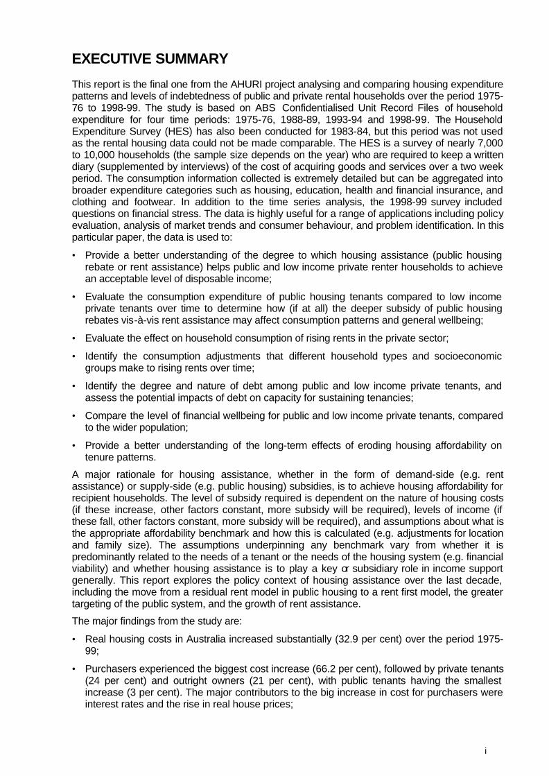
This report is the final one from the AHURI project analysing and comparing housing expenditure patterns and levels of indebtedness of public and private rental households over the period 1975-76 to 1998-99. The study is based on ABS Confidentialised Unit Record Files of household expenditure for four time periods: 1975-76, 1988-89, 1993-94 and 1998-99. The Household Expenditure Survey (HES) has also been conducted for 1983-84, but this period was not used as the rental housing data could not be made comparable. The HES is a survey of nearly 7,000 to 10,000 households (the sample size depends on the year) who are required to keep a written diary (supplemented by interviews) of the cost of acquiring goods and services over a two week period. The consumption information collected is extremely detailed but can be aggregated into broader expenditure categories such as housing, education, health and financial insurance, and clothing and footwear. In addition to the time series analysis, the 1998-99 survey included questions on financial stress. The data is highly useful for a range of applications including policy evaluation, analysis of market trends and consumer behaviour, and problem identification. In this particular paper, the data is used to:

• Provide a better understanding of the degree to which housing assistance (public housing rebate or rent assistance) helps public and low income private renter households to achieve an acceptable level of disposable income;

• Evaluate the consumption expenditure of public housing tenants compared to low income private tenants over time to determine how (if at all) the deeper subsidy of public housing rebates vis-à-vis rent assistance may affect consumption patterns and general wellbeing;

• Evaluate the effect on household consumption of rising rents in the private sector;

• Identify the consumption adjustments that different household types and socioeconomic groups make to rising rents over time;

• Identify the degree and nature of debt among public and low income private tenants, and assess the potential impacts of debt on capacity for sustaining tenancies;

• Compare the level of financial wellbeing for public and low income private tenants, compared to the wider population;

• Provide a better understanding of the long-term effects of eroding housing affordability on tenure patterns.

A major rationale for housing assistance, whether in the form of demand-side (e.g. rent assistance) or supply-side (e.g. public housing) subsidies, is to achieve housing affordability for recipient households. The level of subsidy required is dependent on the nature of housing costs (if these increase, other factors constant, more subsidy will be required), levels of income (if these fall, other factors constant, more subsidy will be required), and assumptions about what is the appropriate affordability benchmark and how this is calculated (e.g. adjustments for location and family size). The assumptions underpinning any benchmark vary from whether it is predominantly related to the needs of a tenant or the needs of the housing system (e.g. financial viability) and whether housing assistance is to play a key or subsidiary role in income support generally. This report explores the policy context of housing assistance over the last decade, including the move from a residual rent model in public housing to a rent first model, the greater targeting of the public system, and the growth of rent assistance.

The major findings from the study are:

• Real housing costs in Australia increased substantially (32.9 per cent) over the period 1975-99;

• Purchasers experienced the biggest cost increase (66.2 per cent), followed by private tenants (24 per cent) and outright owners (21 per cent), with public tenants having the smallest increase (3 per cent). The major contributors to the big increase in cost for purchasers were interest rates and the rise in real house prices;

i

• Real household disposable income for all Australians fell (11.4 per cent), but the bulk of this is explained by changes in household composition (smaller, with fewer income earners) rather than general economic conditions;

• Even allowing for changes in the composition of households, the real income of public tenants fell by 28.7 per cent, and low income private tenants by 9.5 per cent;

• The income effects in public housing are largely related to greater targeting, as evidenced by the increase in households in the lowest two quintiles (from 63.5 to 72.4 per cent), and the proportion of households on at least 90 per cent pensions or benefits (28.2 to 60.3 per cent);

• The combined effect of real increases in housing costs and reduced real incomes means that housing costs consumed 11.7 per cent of household income of all Australians in 1975, but 17.6 per cent by 1999;

• In real terms, the proportion of income committed to housing costs by public housing tenants has increased from 11 to 19 per cent; in 1999 they had $385 disposable income after housing costs, compared to $641 in 1975 (constant 1999 dollars). No other expenditure item experienced increases on the scale of housing;

• For low income private tenants, housing costs increased from 16 to 23 per cent of income;

• The 20-34 year cohort has experienced a sharp fall in home purchasing over the 23 year period (49.0 to 36.4 per cent), which is not compensated by an increase in purchasing rates at a later age. In short, purchasing is in gradual long-term decline. As one could anticipate, this decline is even more rapid in the lowest two quintiles (43.3 to 27.9 per cent);

• Private rental is the long-term growth sector, with 14.4 per cent of the 35-59 age group in this sector in 1975-76, but 18.1 per cent in 1998-99. For the lowest quintiles, the increase was more dramatic: 11.0 to 20.3 per cent;

• In terms of traditional affordability benchmarks, i.e. 25 or 30 per cent of income, this study reaffirms the findings of others that a small percentage of public tenants are in a situation of non-affordability (7.8 per cent for the 30 per cent benchmark), but a large percentage of private tenants (57 per cent). Judged by these measures, public housing works well;

• However, the budget standard measure of wellbeing shows that substantial proportions and absolute numbers of low income tenants, both public and private, cannot live at an adequate standard even after receiving a rebated rent or rent assistance. Traditional affordability benchmarks, which assume a rent first principle of affordability, disguise an inability for many tenants to achieve an adequate standard of living;

• A progressive move from a residual rent model to a rent first model may have protected the financial viability of the public housing system, but it has worsened the position of public tenants. There has been an increase in the proportion of public tenants below the budget standard from 47 per cent in 1975-76 to 64.8 per cent in 1998-99;

• Despite the broadening of eligibility of private tenants’ households to CRA over the 23 year study period and the associated enormous growth in rent assistance, there is no evidence of it making such households in aggregate any better off in terms of disposable income. Of course, without it their position would be even worse;

• The fact that a large proportion of households in 1998-99 were below the budget standard is reflected in the sizeable numbers stating they experience multiple measures of hardship, particularly in terms of being unable to enjoy the things in life most households take for granted, e.g. going on a holiday, having friends or family visit for a meal, being able to put some money aside, buying new rather than secondhand clothes;

• Around 30 to 40 per cent, depending on household type, also experience financial problems such as inability to pay utilities and inability to raise money for emergencies, suggesting an underlying predisposition to rental arrears problems for both public and low income private tenants;

• While the bulk of public tenants (79.0 per cent) and of low income private tenants (62.0 per cent) had no formal debt, a sizeable minority did so, and this was at a level which could

ii

trigger arrears and perhaps loss of tenancy. A disproportionate amount of this debt was with high interest, short loan finance companies;

• For those in debt, the wellbeing measures of missing out, cash flow problems and hardship increased dramatically. This raises issues regarding programs or polices which may enable better debt management or provision for low income earners;

• Two-thirds of public tenants and over half of low income private tenants stated they would be unable to raise $2,000 in an emergency, while those who could do so had a high dependence on families or friends. This suggests how vulnerable such tenants are to any financial crisis, e.g. appliance or car breakdown, funeral, property damage, and therefore to arrears and potential loss of tenancy.

There are many policy implications from these findings. A number are more micro ones, e.g. issues relating to tenants with high debt, but the most problematic policy issue is how do we deal with the fact that current levels of assistance do not appear deep enough to sustain tenants at an adequate standard of living.

In the paper, five broad options are canvassed and discussed:

• Adopt the ‘do nothing’ alternative, acknowledging that a sizeable minority of Australian tenants have to live at below an acceptable living standard, with the social and economic costs that may flow from this;

• Introduce income support reforms which raise pensions and benefits for households to a level whereby they can meet the standard, but with sizeable budgetary implications;

• Restructure public housing rents so that they are set at a level which enables a household to achieve minimum budget standards, i.e. a residual rent model of support more akin to that which characterised the first forty years of public housing. This would however impact on the financial viability of SHAs;

• Create greater opportunities for this low income group to earn labour market income and thereby raise incomes to the level where less direct assistance is required, as hinted at in suggested reforms of the next CSHA;

• Initiate programs, e.g. affordable housing initiatives, to reduce the cost of rental housing so that rent assistance goes further than it currently does in assisting affordability. While important, this does not address a problem of incomes simply being too low to achieve an acceptable living standard, and therefore must be a complement rather than the option.

iii

1. INTRODUCTION

One of the major reasons for government intervention in the housing markets of any society, whether in the form of demand-side (e.g. rent assistance) or supply-side (e.g. public housing) subsidies, is the cost of housing relative to household income. Because this is one of the largest expenditure items in household budgets, high housing costs can push certain households into poverty or force them to compromise the quality or standard of their housing in ways that seriously undermine their quality of life. In the nineteenth and early twentieth centuries, high private housing costs in relation to low labour market income for many people saw widespread poverty and, with the tendency for the poor to congregate in specific areas, the decline of these areas into slums (Harloe 1995; Hayward 1996).

At differing rates and in different forms, advanced industrialised countries – pressured by middle-class social reformers and labour activists at one level, and awareness of the social effects of high housing costs (health, education, work productivity) at another – began to intervene in the housing market (Harloe 1995). Some opted for direct interventions such as rent controls, many for the provision of social housing and, after World War II, many also opted for demand-side subsidies in the form of allowances, vouchers and supplementary payments such as rent assistance. While a leader in many other aspects of social reform (e.g. age pensions, living wage), Australia was a laggard in housing reform, with the consequence that we were relatively late in establishing social housing, and then only in a minimalist or residual form (see Table 1).

Table 1: Tenure by country (early to mid-1990s)

Owner occupied

Private rental

Social rental

United States 70 25 5

Australia 68 22 6

New Zealand 70 24 6

Canada 62 28 6

Belgium 65 28 6

Ireland 78 9 14

Denmark 52 25 18

England 68 10 22

France 56 21 23

Germany 37 38 25

Netherlands 46 13 40

Sweden 40 20 40 Source: OECD (1994) Occasional Paper, no. 14; OECD (1997) Social Statistics; OECD (1998) Occasional Paper, no. 33; NZ Census Statistics 1996; Boelhouwer (1999: Table 1). Note that, for some of the countries, percentages do not add to 100 as they exclude certain housing forms that are difficult to define in terms of tenure, e.g. caravans, boarding houses, holiday homes, shared equity.

Except in war years, rent control has been little used in Australia as a mechanism for controlling housing costs, and demand-side assistance was also minimal up until the early 1980s when a small rent assistance scheme for pensioners was widened in eligibility (Hulse 2002). More money is now spent on rent assistance than on social housing (AHURI 2000: 4), and it has become the major mechanism for dealing with the effects of private market housing costs and associated affordability problems.

Once some form of government assistance is established in order to address high housing costs in relation to income, a decision has to be made as to the degree of subsidy or assistance that should be provided. The level of subsidy required is dependent on the nature of housing costs (if these increase, other factors constant, more subsidy will be required), levels of income

1

(if these fall, other factors constant, more subsidy will be required), and assumptions about what is the appropriate affordability benchmark and how this is calculated (e.g. adjustments for location and family size). The assumptions underpinning any benchmark vary from whether it is predominantly related to the needs of a tenant or the needs of the housing system (e.g. financial viability) and whether housing assistance is to play a key or subsidiary role in income support generally. Among other things, this project assesses changes in housing costs and tenant incomes over time and evaluates the changing nature of subsidy inherent in current and past housing assistance policy.

This research project looks at housing expenditure over the period 1975-76 to 1998-99, particularly for those households in public housing and in the private rental sector on sufficiently low incomes that they may be in receipt of rent assistance (as rent assistance recipients are not identified in the Household Expenditure Survey (HES)). It is not a study of household housing expenditure generally, i.e. home owners, in part because that has already been done (Percival 1998), but mainly because renters receive the bulk of direct housing assistance and are most likely to suffer the effects (e.g. affordability problems) of changes in housing costs. However, as the data offers the opportunity for some broader observations on housing expenditures and trends there, the project makes the occasional excursion into wider housing issues.

2

2. AIMS

This project uses ABS secondary data from the HES to evaluate the effects of housing assistance and public rental on household consumption decisions, and to measure the impacts of increasing private and public rental costs on household consumption decisions, indebtedness and financial stress. More specifically, it aims to:

• Provide a better understanding of the degree to which housing assistance helps low income households to achieve an acceptable level of disposable income;

• Evaluate the consumption expenditure of public housing tenants compared to low income private tenants over time to determine how (if at all) public housing assistance changes consumption patterns;

• Evaluate the effect on household consumption of rising rents in the private sector;

• Identify what sort of consumption adjustments different household types and socioeconomic groups make in response to rising rents over time;

• For key household types or socioeconomic groups in the two sectors (e.g. families with children, the unemployed, different age groups), identify any consumption patterns which may differ from the norm (e.g. expenditure on education) and which may affect ability to participate in society;

• Provide a better understanding of the changing market context in which housing assistance is provided;

• Provide a better understanding of the housing affordability and housing stress conditions confronting low income tenants.

3

3. THE STUDY’S RESEARCH METHODS

Swinburne University, like all universities in Australia, has an agreement with the ABS to access its Confidentialised Unit Record Files (CURFs) for approved non-commercial purposes. These are the most detailed data that can be released from an ABS survey and enable the researcher to cross tabulate and organise the data in any way they like. For example, with the HES data, we are able to create a group of private tenant households who rely primarily on a statutory income and pay more than a certain amount on rent, and compare their expenditure patterns and level of household indebtedness to households on statutory incomes in public rental.

The HES collects information on the expenditure, income and characteristics of households resident in private dwellings throughout Australia. It is a survey of nearly 7,000 households who are required to keep a written diary (supplemented by interviews) of the cost of acquiring goods and services over a two-week period. The consumption information collected is extremely detailed (e.g. there are nine gambling items) but can be aggregated into broader expenditure categories such as housing, education, health and financial insurance, and clothing and footwear. The data is highly useful for a range of applications including policy evaluation, analysis of market trends and consumer behaviour, and problem identification. Just as expenditure items are very detailed, so is the household income data, including the many categories of government payments. Although rent assistance is not a discrete payment category, cross-tabulating rent paid with source of income will enable a category of (likely) rent assistance recipients to be identified.

The HES has been conducted in 1975-76, 1983-84, 1988-89, 1993-94 and 1998-99, providing a rich database of expenditure and income patterns which enables a detailed investigation of changes over time. In addition to the time series analysis, the 1998-99 survey also included questions on financial stress. These are analysed to find out the degree to which public and private tenants experienced such stress, whether there were differences between the two tenant types, and whether there were differences across household types.

Of course, for such a long time series there will always be continuing changes to the data collection process that affect comparability. The most important is that the 1983-84 survey did not distinguish between public and private rental, with the result that this time period has not been included in the analysis. The study adhered to the same data correction principles as NATSEM (Percival 1998), with some changes, notably to the 1998-99 data which was not available at the time of Percival’s study. These are:

• The 1975-76 HES includes an amount for repaying the principal component of a mortgage, as distinct from the interest component. This was not done in subsequent years. As the study only concerns itself with rental, this is not a problem;

• In 1975-76 and 1983-84, negative incomes were set to zero by the ABS. Accordingly, negative incomes in subsequent years have also been labelled zero;

• As the pre-1993-94 HES did not include the Northern Territory, it has also been excluded from the national aggregates for 1993-94 and 1999-99;

• The 1998-99 HES changed the definition of dependent children over the age of 15 to include full-time students aged 15-24 who have a parent in the household, where in previous surveys it included full-time students aged 15-20 who have a parent in the household. Where possible, the 1998-99 data has been adjusted to the same measure as other years.

There have also been some changes to sample sizes and the balance between areas, as summarised in Table 2.

4

Table 2: Differences between HES sample sizes

Geographical area 1975-76 1888-89 1993-94 1998-99

Capital city 2,813 5,263 6,107 4,795

Other urban area 2,225 1,630 1,712 1,534

Rural 831 512 570 564

Total 5,869 7,405 8,389 6,893 Source: ABS 2000, Household Expenditure Survey Australia: User Guide 1998-99: 22.

In order to make relevant comparisons between groups, i.e. to exclude more affluent tenants, private tenants in the two lowest income quintiles have been used to compare with public tenants. In some situations, e.g. comparison of all tenures, the two lowest quintiles have been used for both private and public housing. In all other quintile comparisons, it is the lower quintiles of all households, not the lower quintiles within each tenure group. This could mean, for example, that we are comparing over 50 per cent of all public housing tenants with just 20 per cent of purchasers, as a larger proportion of lower quintile groups are in public housing and private rental, and a much smaller proportion are purchasers. The quintile income was calculated for each household type, and then the number below this income in each type determined. This method was used instead of striking an average quintile income across all households and determining how many households’ income fell below this.

The income data also excluded households who nominated having zero to less than $30 per week (in 1998-99 prices) as not being meaningful in terms of respondents misunderstanding the income data or who had arranged their affairs, e.g. taxes, such that they had minimum income. Discussions with the ABS suggest that the latter occurs among higher income earners and therefore to include them in the lowest income quintiles would distort the data. The ABS is itself considering adjustments to future income data sets along similar lines.

The public housing sample in 1998-99 is 529 households, which produces a sample error rate around 9 per cent. In earlier years, with higher samples, the error rate is closer to 5 per cent. Private tenants, of whom there were 962 in 1998-99 and more in other years, have an error rate of 2.5 per cent, while for lower income tenants (around 500) the rate is 9 per cent.

In addition to the information regarding expenditure, income and household characteristics, the latest HES (1998-99) included a series of questions based on recent living standards research, covering topics such as management of household income, present standard of living compared with two years ago, ability to raise emergency money, main source of emergency money, and cash flow problems. These subjective measures of economic wellbeing provide another basis of comparison for low income households in the private and public rental sectors.

Use of HES unit record data is not an easy task and requires considerable recoding and creation of new variables. One key methodological problem is that the data does not identify rent assistance recipients, so low income private tenants (i.e. those whose income would enable them to qualify for rent assistance) are used as a proxy throughout this study.

The HES is used in most countries as the primary data source for updating their Consumer Price Indexes and revising the category of goods and services that make up the CPI basket, as well as for changing the weighting of items. It is also used to evaluate the effects of government payments (e.g. pensions and allowances) on income distribution and household wellbeing. Its use in housing-specific research in Australia and internationally has not been great, and it is most commonly used by economists for estimating housing elasticities, that is, changes in the supply or demand of a commodity or service in response to changes in incomes. For a summary of the methodological problems and findings on elasticity research, see Ermisch, Findlay and Gibb (1996) and Hansen, Formby and James Smith (1998).

The following section pays particular attention to different methods of measuring housing affordability and outlines the budget standards method, which is essentially a method of determining affordability based on an acceptable minimum standard of housing expenditure consistent with a modest budget, rather than by poverty lines or arbitrary benchmarks such as 25 or 30 per cent of income.

5

4. MEASURING HOUSING AFFORDABILITY

The HES time series data lends itself to analysis of housing affordability and benchmarks of affordability, that is, how much of a low income household budget should housing consume, and therefore how much should be subsidised for such households. Some discussion of methods of measuring affordability is therefore necessary, given that different methods are based on different assumptions and therefore yield different results. There have been other studies or reports that have given attention to the problems of measuring affordability, most notably King (1994) and Bray (1995). This paper adopts a different perspective and includes a new method of measuring affordability not discussed in either of these papers. It focuses more on assumptions and principles and the historical origins of the methods, and also includes implications for social housing and private rental rent setting and rent assistance policies. Other than simply identifying them, the technical issues around different measures of affordability are not discussed, as the King and Bray studies do this more than adequately.

4.1. Shelter First: Housing Costs as a Proportion of Income This approach is the most common in terms of affordability measures and relates the housing costs of a person or household to their income in percentage terms. Technical problems include whether income should be before or after tax, whether housing subsidies, e.g. rent assistance, should be counted as part of a household income to which housing costs are related, and, if trying to measure affordability for low income households, what is an appropriate definition of low income, for example, is it a household in the lowest 10, 20 or 40 per cent of income earners. The other major issue around the proportional method is less a technical one than a conceptual or philosophical one, i.e. what is the benchmark proportion that is considered acceptable in a society, and how much should people pay by way of housing costs. There is no right or wrong answer to this question. The rationales or justifications are as much philosophical judgements based on a society’s values and its historical and institutional structure. In Australia the longest established benchmark would appear to be 25 per cent (see below), although the National Housing Strategy of 1991 put up 30 per cent as a benchmark and this has been used as an alternative since then.

Historical Rule of Thumb

One rationale for the 25 per cent benchmark is based on a rule of thumb that housing costs are normally around a quarter of a household’s income. This is not sophisticated evidence based policy, but appears to have emerged from historical observation of people’s housing practices and financial institutions’ lending practices. It underpinned the National Housing Strategy (NHS 1991). While the NHS study documented the scale of the affordability problems nationally – that is, more than 10 per cent of households in housing stress (defined as paying more than 25 or 30 per cent of their income on housing costs) – it also had the effect of consolidating 25 and 30 per cent as benchmarks for affordability in Australia. Since then, policy discussion has conventionally used these as the lower and upper measures of the appropriate housing costs to income ratio, and public housing authorities have moved the rebate to the 25 per cent benchmark. However, the NHS only gave cursory attention to the rationale for this benchmark, providing a brief overview of what some other countries set in terms of benchmarks (many are much lower) and then apparently choosing an upper end benchmark of 30 per cent, the Canadian core housing needs model. The upper end benchmark was also seen to fit contemporary practices in terms of home ownership lending conditions by financial institutions (NHS 1991: 6-7). A historical review of the North American origins of the ‘right’ amount of income to spend on housing also found that it was largely grounded in banking practices and could be traced back to the 1920s and 1930s. It was also based on some rough and ready judgements of what an average low income worker spent on rental housing in North American cities. Both suggested 25 per cent (Feins and Lane 1981). However, such rule of thumb benchmarks are set by private market requirements, not necessarily by what a household can afford. In the private market, a household could be measured to be living in an affordable situation using such a benchmark, but may only be able to do so because, for example, there are four of more household members to a two bedroom dwelling. Affordability is achieved, but at the expense of overcrowding. Similarly, such benchmarks typically fail to recognise the needs of different family types. If a single person paid $200 a week rent out of a gross income of $800, and a family of five

6

paid the same amount (25 per cent in both case), can they be treated as being in equivalent affordability situations? The former may have more than enough to live on after meeting housing costs, the latter may not, yet the 25 per cent benchmark treats them as one and the same. A major assumption of 25 and 30 per cent benchmarks is that rent payments have first claim on a household’s budget, i.e. a public housing tenant is expected to pay at least 25 per cent of their income in rent and if this does not leave enough for other essential expenditures then that is an income – not a housing – problem. This assumes that housing is not a key component in any income security system, and that income supplements are the appropriate way to ensure adequate standards of living, not housing.

4.2 Non-Shelter First Claim An alternative approach to affordability is to assume that other expenditure items have first claim on the budget, and housing cost should be the residual. This was often used as the principle in setting rents in socialist societies and, as we shall see, was influential in rent setting practices of the early public housing system in Australia. Academically it has been given the most attention by Stone (1993). The principle of measurement is simple. If the necessary expenditure for all other items is identified, then what is left over is how much is available for rent. This should be how much people pay. This approach assumes that housing programs should be the instrument for addressing all income problems; that is, that housing is the linchpin for a social security system. This might, for example, create a requirement that rents should be around 9 per cent of income (Stone 1993). There are two methods for broadly determining a non-shelter first measure of affordability: that of the poverty line and that of a budget standard.

The Poverty Line

In Australia the most commonly used non-shelter first method of affordability is the Henderson poverty line, established by the Commission of Inquiry into Poverty (chaired by Ronald Henderson) in 1974-75. The method was to identify that level of income necessary to afford a certain minimum standard of living. It was based on a number of doubtful assumptions and, while it is criticised for not reflecting contemporary standards of living and associated costs, it is updated quarterly by the Institute of Applied Economic and Social Research at the University of Melbourne, and until recently was the only measure for evaluating the non-shelter first concept of affordability (Maher and Burke 1993). The Henderson poverty line deducts a certain amount for housing costs, which varies for different household types. The assumed housing costs (see Table 3), particularly as they apply to private rental, would understate actual costs in most parts of contemporary Australia.

Table 3: Housing cost components of Henderson poverty line, June 2002

Single Assumed housing cost

Couple Assumed housing cost

No dependents $97 No dependents $106

One dependent $106 One dependent $116

Two dependents $116 Two dependents $126

Three dependents $126 Three dependents $135

Four dependents $136 Four dependents $146 Source: Melbourne Institute of Applied Economic and Social Research (2002)

There are two ways the Henderson poverty line can be used as a measure of affordability. One is to take it including housing costs and compare actual incomes with the poverty line; the other is to do the same but exclude housing costs which then enables, by comparison, an evaluation of the effects of housing costs on accentuating or mitigating poverty.

7

Budget Standard

This method assumes that housing programs should be designed to reduce housing costs to an amount that leaves sufficient left over to cover an acceptable minimum standard of expenditure consistent with a modest budget. On the principles of this model of affordability, housing is just one part of a set of programs that address social security issues. The method here is to identify an acceptable standard of housing expenditure as a basis for setting a general housing cost to income ratio. This might be anywhere between 15 and 30 per cent, depending on household type and location and the bundle of other household expenditures. Until recently there has been no budget standard in Australia to evaluate the effects of housing affordability against, hence the use by default of the Henderson poverty line. In 1998 the Social Policy Research Centre (SPRC) at the University of New South Wales developed indicative budget standards for Australia and these are now a more robust alternative to the poverty line (Saunders et al. 1998).

4.3 Non-Shelter First to Shelter First: Rent Setting and Affordability in Public Housing When the states and territories first established their public housing systems, a key policy issue was the effective level of rent that tenants should pay. The methods were a combination of rule of thumb and budget standard. Justice Higgins’ determination in his Harvester Judgement of 1907 set a living wage based on what an unskilled labourer required to meet the normal needs of himself, his non-working wife and three children. He found that rent constituted 7s or one-sixth of a weekly wage of 42s (McNelis 2001: 38). In his successful push to establish the Victorian Housing Commission, social reformer Oswald Barnett argued that there was a need for an economic rent (i.e. one which covered the cost of a dwelling) and an ‘ability to pay’ rent which ‘must bear a relation not only to family income but also the number in the family unit’ (Barnett and Burt 1942).

The report of the Housing Investigation and Slum Abolition Board (of which Barnett was chairman) used these two notions, supplemented by a review of English rent schemes and the findings of the Harvester Judgement, to recommend an economic rent of 22 per cent of income for a family on the basic wage. This was higher than Higgins’ 15 per cent, but should be seen as an equivalent, given that the public housing economic rent was considerably less than private sector market rents. However, 22 per cent was the upper benchmark, and for every 3s below the basic wage the rent was reduced by 1s per week. Moreover, the family income was to be further reduced by 7s 6d for each fourth and subsequent child. These combinations meant that the rent to income ratio could be anywhere between 9 and 22 per cent but, for a typical lower income household (e.g. one on an income of 80 per cent of the basic wage or with one additional child), the ratio was 18 per cent (HISAB 1938).

These principles, if not the details, were largely adopted by the Victorian Housing Commission and formed the basis for the Commonwealth Housing Commission’s recommendations of 1944 which in turn led to the first CSHA a year later (McNelis 2001: 45). This laid the foundations for all subsequent social housing provision. Clause 11(1) set the benchmark for rebate of rents at one-fifth of family income equal to the basic wage, with families whose income was less than this receiving a further rebate by one quarter for any amount below the basic wage. Rebates decreased by one-third for any amount above the basic wage. The income to which the rent related was defined as the whole of the income of the highest income earner, two-thirds of the next highest earner’s income, and one-third of other household members’ income up to some maximum, then set at 30s.

While the income definition changed over time, the rent to income ratio was still broadly operative in 1991 at the time of the NHS and was only changed in the 1998 CSHA. Interestingly, the one-fifth benchmark had been a compromise as the 1944 report actually recommended one-sixth as the benchmark (McNelis 2001). Thus, for most of the postwar period, the rent to income ratio was structured in a way which, depending on income and family size, meant that the appropriate percentage could be anywhere between 15 and 25 per cent. For those on higher incomes and paying the full economic or cost rent, it could be as much as 25 per cent of income, but for lower income earners it was more likely to be between 15 and 20 per cent. With some state and territory variations, we are now looking at a policy environment where 25 per cent (i.e. the NHS affordability benchmark) is used by both public and community housing, at least for new tenants.

8

Looking at this history, we can hypothesise that both the 1991 NHS and 1998 CSHA benchmarks were chosen less as measures based on housing need, but to minimise the potential budget costs of low income housing assistance and to keep public housing agencies financially viable in a context of more and more households receiving a rebate and of contracting real expenditure on public housing. What started out in public housing as rents being set to leave enough for day to day living has now become a rent first system. This study will evaluate whether the current affordability ratios are appropriate from a household’s, rather than systems maintenance, perspective.

It may well be that a flat rebate of 25 per cent for all household types is inappropriate and that, as with the original Commonwealth Housing Commission recommendation and early public housing practice, there need to be more differentiated measures. Feins and Lane (1981: 65), for example, using United States data, found on the basis of actual housing expenditure patterns of different types of low income households that 19 per cent of income was appropriate for larger family types, but for older couples it could go up to 36 per cent. The Australian context may mean different outcomes, but this illustrates the point that different household types and potentially different locations might mean different affordability ratios.

4.4 Budget Standards: The Methodology One important use of the household expenditure data is to evaluate whether housing costs have risen for low income households to the degree that it affects their ability to maintain an acceptable standard of living. The problem here, and one with a long tradition in social policy research, is identifying and finding a measure of what represents such a standard. There are two broad approaches to resolving this problem. One is to focus on the income necessary to achieve a certain standard of living, typically measured by a poverty line set as some relationship (e.g. median or mean) to national average earnings. The other, and one given less attention in Australia, is to focus on the level of consumption consistent with a certain standard of living.

Methodological issues around the former have recently received prominent media attention. A Smith Family/NATSEM report defined poverty as those households receiving less than half the mean income. By this criterion, 13 per cent of Australians in 1999 were in poverty, up from 11.3 per cent in 1990. Tsumori, Saunders and Hughes (2002) criticised this measure because of its sensitivity to changes in the mean income caused by increases at the top end of the range. If the median income, which is less sensitive to growth in outliers, was used, then poverty would have been lower, but they see even this as still too much a relative concept linked to other people’s income.

The alternative to an income measure of poverty is some form of consumption based measure which attempts to define a minimum acceptable budget standard (Bradshaw 1993; McDonald and Brownlee 1994). Such a measure is available in Australia, although rarely used and not given the policy attention it deserves. Between 1995 and 1998 the SPRC worked on developing indicative budget standards for Australia. Their results will be used in this study so therefore warrant explanation.

A budget standard represents ‘what is needed, in a particular place at a particular point in time, in order to achieve a specific standard of living’ (Saunders et al. 1998: 4). The report is prefaced by a discussion of the considerable conceptual and methodological problems involved. It acknowledges that a budget standard has to be defined by someone and is therefore subjective.

The SPRC approach is essentially twofold: firstly, the patterns of the ABS HES are used to get a measure of the weight and cost of expenditure items in household budgets; secondly, normative judgements of the research team backed up by focus group discussions were used to set the amount needed for different household types. These methods were highly specific, working through detailed expenditures within categories of housing, energy, food and drink, clothing and footwear, household goods and services, health, leisure, transport and personal care.

Two standards were established: a modest but adequate one, and a low cost one which is a level of consumption that may require frugal and careful management of resources – that is, a subsistence level budget that may involve serious compromise in expenditure related to areas such as health and education (Saunders et al. 1998: 63). For the purposes of this study, the low cost standard has been used in order to ward off any challenges of excessive needs. It differs from the modest but adequate standard by costing some items at a cheaper price, by

9

incorporating lower quality products or fewer of them, by extending lifetimes (e.g. for durables) or by excluding some items altogether.

The analysis was done for a limited range of households. Fortunately, the households modelled included those that make up the major client groups of the rental sector.

The housing component of the minimum budget standard was based on public and private rents for the Hurstville area of suburban Sydney, with the rent rebated for the public sector at the rates relevant for the different household types (assuming some minimum income). In the analysis used in this study, actual private and public rents from the 1998-99 HES were substituted for these surrogate values.

10

5. FINDINGS

5.1 Income and Housing Cost Data To date, little use has been made of the HES CURF data for housing research, the major exception being the paper by Richard Percival (1998) on which this project partly piggy-backs. His paper analysed housing expenditures for time period 1975-76 to 1993-94, with modelling of the data to extend the analysis to 1997. It was a study which looked at broad housing expenditure trends across all tenures. By contrast, this study extends the actual HES time period to 1998-99, mainly focuses on lower income rental households, includes data for the states and ACT, and includes analysis of variables ignored by Percival.

However, while the focus is narrower and deeper than Percival’s, it is useful to locate the study in the broader context of housing consumption trends generally.

Our starting point is the changes in the real cost of housing for all Australians over the 23 years of the study period. This is measured by housing related expenditures which include rents and mortgages but also repairs, house and content insurance and any service charges. They are thus not equivalent to rents or mortgages, although these typically account for the bulk of expenditures.

Figure 1: Australian mean housing cost, 1975-76 – 1998-99 (constant 1999 dollars)

$140

$120

$100

$80

$60

$40

$20

$0

1976 1988 1993 1998

$96

$109

$122$128

$71 $75

$82 $85

All

2nd Quintile

Year

Figure 1 shows a 32.9 per cent increase in the real cost of housing, from $96 per week in 1975-76 to $128 per week in 1998-99. This is an average cost across tenures that have very different consumption attributes and cost structures. It could thus represent an actual cost of housing through, say, higher mortgage costs, land costs, rents etc., or it could represent a change in the compositional make-up of the tenures so that there were more households in those demographics living in a high cost tenure (e.g. home purchasers) than in a low cost tenure (e.g. outright ownership). Table 4 suggests something of the explanation.

Table 4 shows that all tenure sectors contributed something to the increase, but the two most important were purchasers (up 66.2 per cent) and private rental (up 24.7 per cent). For purchasers, most of this increase was in the cost of a mortgage (Percival 1998: 10). However, this does not take us far, as the increased cost could be because of higher interest rates, a higher mortgage requirement because of higher property values, or a higher mortgage requirement because of consumption changes (e.g. a switch to larger and more expensive houses). Note that the increase in purchasing costs was between 1975-76 and 1993-94, and that in real terms they fell slightly by 1998-99.

Am

ou

nt

Sp

ent

on

Ho

usi

ng

11

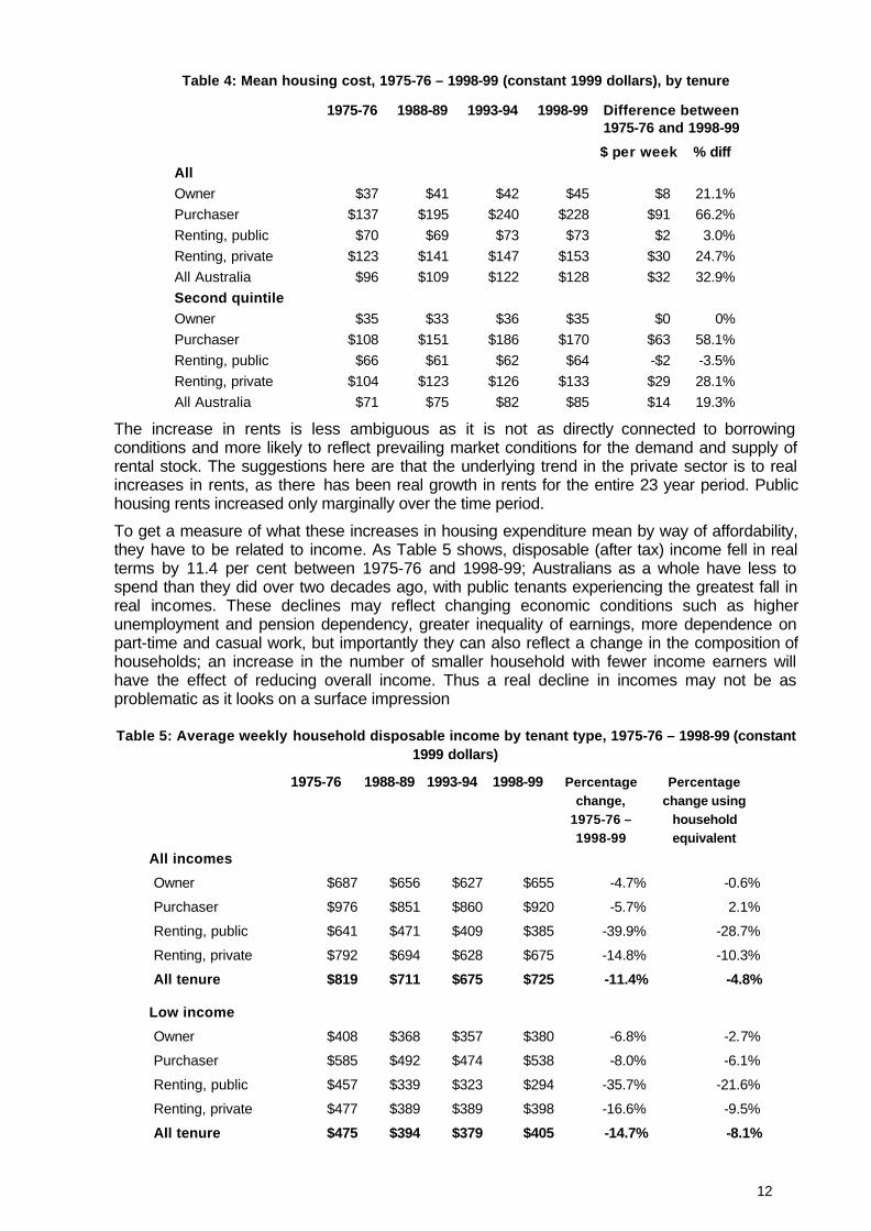
Table 4: Mean housing cost, 1975-76 – 1998-99 (constant 1999 dollars), by tenure

1975-76 1988-89 1993-94 1998-99 Difference between

All Owner Purchaser Renting, public Renting, private All Australia Second quintile Owner Purchaser Renting, public Renting, private All Australia

1975-76 and 1998-99

$ per week % diff

$37 $41 $42 $45 $8 21.1% $137 $195 $240 $228 $91 66.2% $70 $69 $73 $73 $2 3.0%

$123 $141 $147 $153 $30 24.7% $96 $109 $122 $128 $32 32.9%

$35 $33 $36 $35 $0 0% $108 $151 $186 $170 $63 58.1% $66 $61 $62 $64 -$2 -3.5%

$104 $123 $126 $133 $29 28.1% $71 $75 $82 $85 $14 19.3%

The increase in rents is less ambiguous as it is not as directly connected to borrowing conditions and more likely to reflect prevailing market conditions for the demand and supply of rental stock. The suggestions here are that the underlying trend in the private sector is to real increases in rents, as there has been real growth in rents for the entire 23 year period. Public housing rents increased only marginally over the time period.

To get a measure of what these increases in housing expenditure mean by way of affordability, they have to be related to income. As Table 5 shows, disposable (after tax) income fell in real terms by 11.4 per cent between 1975-76 and 1998-99; Australians as a whole have less to spend than they did over two decades ago, with public tenants experiencing the greatest fall in real incomes. These declines may reflect changing economic conditions such as higher unemployment and pension dependency, greater inequality of earnings, more dependence on part-time and casual work, but importantly they can also reflect a change in the composition of households; an increase in the number of smaller household with fewer income earners will have the effect of reducing overall income. Thus a real decline in incomes may not be as problematic as it looks on a surface impression

Table 5: Average weekly household disposable income by tenant type, 1975-76 – 1998-99 (constant 1999 dollars)

1975-76 1988-89 1993-94 1998-99 Percentage Percentage

All incomes

Owner

Purchaser

Renting, public

Renting, private

All tenure

Low income

Owner

Purchaser

Renting, public

Renting, private

All tenure

change, change using 1975-76 – household 1998-99 equivalent

$687 $656 $627 $655 -4.7% -0.6%

$976 $851 $860 $920 -5.7% 2.1%

$641 $471 $409 $385 -39.9% -28.7%

$792 $694 $628 $675 -14.8% -10.3%

$819 $711 $675 $725 -11.4% -4.8%

$408 $368 $357 $380 -6.8% -2.7%

$585 $492 $474 $538 -8.0% -6.1%

$457 $339 $323 $294 -35.7% -21.6%

$477 $389 $389 $398 -16.6% -9.5%

$475 $394 $379 $405 -14.7% -8.1%

12

To test the degree to which changes in income are a function of compositional rather than economic circumstances, household disposable income can be adjusted for compositional effects by the application of equivalence scales for each household type. To put it simply, this is a statistical method for creating a household income which takes account of the different needs of households with different compositions by saying the equivalent need can be measured by the square root of the number of persons in the household. Using this method, the overall rate of fall in real incomes for each tenure category is reduced substantially compared to the non-equivalent scale method. This is highlighted by the last column of Table 5. Thus, once homeowners’ compositional effect is accounted for, they only had a -0.6 per cent fall, while purchasers actually had a minor increase in income. Public and private tenants continued to experience falls in real income, even allowing for changes in composition and, in the case of public tenants, to the tune of nearly 30 per cent. These falls in income suggest that any real cost in housing expenditure would cut severely into a public or private tenant’s household budget and affect their capacity to maintain expenditure standards. Table 5 also shows that the fall in all tenure disposable income was arrested after 1993-94 and increased slightly to 1998-99, although for public tenants the decline has continued.

As an aside, it is interesting to compare the income differences between public housing tenants in Australia and social housing tenants in other countries as a result of the decline in incomes. In Australia public housing tenants’ incomes by the late 1990s were equivalent to 53 per cent of average household earnings, whereas in France, Germany, the Netherlands and Sweden tenants all have incomes of at least 70 per cent of average income (Stephens, Burns and McKay 2002). British social tenants, however, share the low relative incomes of Australian public tenants largely because, as in Australia, the system is geared to a safety net function and – as we shall see in the Australian context – even this is a very holed safety net. Nevertheless, British public tenants still pay a lower proportion of their total expenditures on housing than their Australian equivalents (16 per cent c.f. 19 per cent). In Australia, outright ownership consumes less of the household budget than in the United Kingdom (7 per cent c.f. 10 per cent ), house purchasing consumes more (23 per cent c.f. 17 per cent), and private rental is the same at 23 per cent (United Kingdom Statistical Office 2001).

In the case of public tenants, the substantial decline in their real income is no doubt explained by greater targeting and a move to market rents which had removed many higher income earners from public housing by the late 1990s. Both the Commission of Inquiry into Poverty (1975) and Jones (1972) drew attention to the relatively small numbers of poor people in public housing and helped to create a policy climate that led to ongoing reforms to eligibility and allocations. We can see the effects: in 1975-76 the average disposable income of a public housing tenant was equivalent to 78 per cent of the total average disposable income for all households; in 1998-99 it was down to 53 per cent.

Evidence of the effect of targeting is in the proportion of those in the lowest quintile over time. As Table 6 shows, there has been a steady increase in the proportion of public tenants in the lowest disposable income quintile for each of the HES survey years, reaching 72.4 per cent by 1998-99. By comparison, the ownership tenure has shown some decline (reflecting the need for a higher income if one is to be an owner), while private rental has also seen some increase (to 36.9 per cent).

Table 6: Proportion of households below second quintile by tenure, 1975-76 – 1998-99

Tenure 1975-76 1988-89 1993-94 1998-99

Owner 52.4 47.4 47.7 49.4

Purchaser 30.1 26.2 24.6 25.2

Renting, public 63.5 67.8 69.2 72.4

Renting, private 33.6 35.1 35.8 36.9

Total 40.4 39.9 40.3 40.4

13

Further evidence around the targeting story is provided by Figure 2 which looks at the two rental tenure categories by the proportion who are almost solely pension and benefit dependent (90 per cent plus) and those who are 50 to 90 per cent dependent. Between 1975-76 and 1998-99 the proportion of public tenant households who are solely pension dependent rose from 28.2 to 60.3 per cent, and the proportion of low income private tenants from 23.1 to 49.6 per cent. By contrast, among all households (including ownership), the proportion increased to 21.4 per cent by 1993-94 but fell back to 18.7 per cent by 1998-99. We can conclude that the proportion of the Australian population who are dependent on 90 per cent plus benefits appears to have peaked, but that they are becoming ever more concentrated in public and low-end private rental housing.

Figure 2: Proportion of households on benefits by tenure, 1975-76 – 1998-99

0

10

20

30

40

50

60

Renting, public Renting, private All Aust Renting, public Low Income Private Rent

All Aust

Between 50% and 90% of income from benefits More than 90% of income from benefits

1976

1988

1993

1998

Targeting means that there are more and more households in the public rental sector who are unable or unwilling for whatever reason (age, disability, social skills, education, childcare) to be in the workforce earning an income. The differences between tenure areas are sharp. Table 7 shows the labour force status of the principal income earner in the HES households in each tenure, excluding those who are on an age or disability pension. It shows that 58.7 per cent of all public tenants are not in the labour force, compared to only 6.3 per cent of all purchasers and 22.3 per cent of all private tenants. The average for all tenures is 15.9 per cent. By controlling for income, in the sense of looking at all households in the two lowest quintiles, the differences are reduced but not greatly. It shows that 38.2 per cent of all households in the lowest quintile do not have the principal income earner employed. For purchasers, however, it is only 33.3 per cent, and for public tenants it is 76.8 per cent. Given that all these income earners are in the same broad income category, this raises the questions of what factors other than income are operative in shaping ability to participate in the workforce and seek out different tenure outcomes. As age and disability have been controlled for, the reasons must have more to do with other factors. The exploration of these factors is, however, beyond the domain of this project and could well be another research topic.

14

Table 7: Number of unemployed persons per household by tenure, all households

Tenure Principal income earner Principal income earner (low quintiles)

% not in workforce

Number % not in workforce

Number

Owner 15.9 318,722 33.3 226,010

Purchaser 6.3 128,399 19.6 95,805

Renting, public 58.7 139,502 76.8 108,221

Renting, private 22.3 329,860 52.2 256,646

All 15.9 916,484 38.2 686,682

Table 8 shows the trends in housing expenditures for public and private tenants by income quintiles, revealing a somewhat divergent pattern. Private rental housing expenditures are spread remarkably evenly, with all quintiles experiencing broadly similar levels of increase of 20 to 30 per cent over the time period. Public renting had a more varied performance, with a contraction in rents for the lowest quintiles and increases for the highest quintiles, no doubt reflecting the rent to income formula of state housing authorities such that with more very low income groups in the lowest quintiles in later years (the targeting effect) then rents would be expected to fall.

Table 8: Weekly household expenditure on housing, public and private tenants, disposable

Renting, public

1st quintile

2nd quintile

3rd quintile

4th quintile

5th quintile

Renting, private

1st quintile

2nd quintile

3rd quintile

4th quintile

5th quintile

income quintiles

1975-76 1988-89 1993-94 1998-99

Count Mean Count Mean Count Mean Count Mean

63,770 $64 131,338 $60 218,408 $57 205,113 $61

75,275 $68 99,915 $62 95,468 $72 70,667 $73

35,645 $70 53,352 $74 68,283 $85 68,289 $89

30,867 $79 28,307 $87 51,634 $109 30,670 $108

15,172 $90 28,145 $103 22,614 $101 6,420 $91

Count Mean Count Mean Count Mean Count Mean

132,658 $110 167,352 $123 232,446 $123 277,175 $133

145,648 $99 177,341 $123 257,831 $128 308,648 $134

150,407 $135 175,032 $141 295,040 $144 294,067 $144

230,232 $124 239,748 $149 328,669 $149 398,249 $156

179,059 $138 216,395 $160 272,271 $187 309,002 $194

What is the outcome when housing cost and income trends are combined? Figure 3 shows the combined effect of real declines in income and dwelling price changes in terms of the amount of disposable income available for other goods and services available for public and private tenants. Whereas in 1976 all public tenants had an average $641 of disposable income, by 1998 this had fallen to $385, a 39.9 per cent decrease. The average for all private tenants fell from $792 to $675, a 14.8 per cent decrease, but low income private tenants (the two lowest quintiles) fell more sharply from $477 to $398, a 16.6 per cent decrease.

Figure 3 also shows the progressive increase in the amount of total household disposable income which is consumed by housing. For public tenants this has risen from 11 to 19 per cent, while for low income private tenants it has gone from 22 to 33 per cent.

15

100%

90%

80%

Figure 3: Amount of disposable income after housing costs (constant 1999 dollars)

$70 $69 $73 $73 $104 $125 $126 $133

$123 $141 $147 $153

$571 $402 $293 $313 $377

$266 $265 $265

$670 $553 $414 $522

1976 1988 1993 1998 1976 1988 1993 1998 1976 1988 1993 1998

Renting, public Renting, private(low income) Private renter all

11% 15%

20% 19% 22%

32% 32% 33%

16%

20% 26%

23%

70%

60%

50%

40%

30%

20%

10%

0%

Tenure

Housing expenses Remaining Income T

able 9 shows the changes in public and private rental (lowest quintiles) housing expenditures for each state and territory over the 23 year period. It reveals quite marked divergence around the national real increase of 3 per cent. Queensland and South Australian public tenants actually experienced real declines, in Queensland’s case by 15 per cent, while the others ranged from a 2.9 per cent increase (ACT) to 14.4 per cent (WA). Unlike in the private rental sector, public sector rents are not a market outcome. Differences between states and territories rather reflect an interaction between changes to rent setting formulas and the composition of tenants with their associated differences in income. Rent trends are derived from the outcome of these other processes and are not independent variables in their own right.

Private rental housing cost trends are the product of market processes and, while the overall trend is to substantial real increases (28.1 per cent Australia-wide), there is sharp variation around the trend. As one might expect, NSW experienced increases above the national trends, but not to the degree of Queensland, which has a 72 per cent real increase. Some of this could reflect the state’s strong economic growth over this period, but is also likely to mirror the substantial decline in low cost rental stock identified by Wulff, Yates and Burke (2001). Tasmanian private rents also grew substantially. Much of this could be an adjustment to the extremely low rents of 1975-76, as even despite the 66.9 per cent real increase, rents are still below the national average.

Table 9: Average housing costs: renting public and private rental, lowest two quintiles (constant 1999 dollars)

Renting, public Renting, private (low income)

1975-76 1998-99 % diff 1975-76 1998-99 % diff

NSW $67 $72 7.9% $112 $145 29.5%

Vic $82 $89 8.9% $118 $124 5.4%

Qld $78 $66 -15.1% $80 $137 72.0%

SA $70 $69 -1.8% $90 $107 19.3%

WA $59 $68 14.4% $86 $122 41.5%

Tas $55 $59 7.2% $76 $126 66.9%

ACT $84 $86 2.9% $166 $148 -10.8%

Aust $70 $73 3.0% $104 $133 28.1%

The position with disposable incomes is more consistent (see Table 10), with all states and the ACT experiencing real falls in both the private and public sectors. In public housing, Victoria is the exception, where disposable income did not fall to the same degree. Given that Victoria led the charge with targeting, this is hard to explain, as it also means that in 1998-99 the average

16

disposable income of Victorian public tenants was higher than in all other states and the ACT. Tasmania, by contrast, has the lowest average disposable income. In private renting, there was a general consistency of decline, with the exception of Queensland where disposable incomes have held up better, only falling 2.9 per cent compared to the national fall of 16.6 per cent.

Table 10: Disposable real income, renting public and private rental, lowest two quintiles (constant 1999 dollars)

Renting, public Renting, private (low income)

1975-76 1998-99 % diff 1975-76 1998-99 % diff

NSW $699 $363 -48.% $470 $409 -12.9%

Vic $576 $483 -16% $507 $368 -27.4%

Qld $757 $371 -51% $444 $432 -2.9%

SA $554 $359 -35% $512 $378 -26.2%

WA $550 $413 -25% $463 $361 -22.1%

Tas $469 $282 -40% $439 $333 -24.1%

ACT $838 $450 -46% $501 $448 -10.5%

Aust $641 $385 -40% $477 $398 -16.6%

Combining the housing cost and income effects, we see in Table 11 the percentage of disposable income consumed by housing costs (largely rents). In public housing the proportions are not greatly dissimilar, illustrating that by the 1990s each jurisdiction had broadly the same allocations and rent setting policies. All jurisdictions in 1998-99 had housing cost to disposable income percentages in the 20s, whereas in 1976 they had ranged from 11.6 to 18.0 per cent. In private rental the housing cost/income effect has been most problematic for Tasmania. Because of lower real incomes and substantial increases in real rents, the ratio of rents to disposable income is worse than that of NSW. One message here is that there is a trend towards a long-term affordability problem across all states and territories. It is not, as some might think, a Sydney or NSW problem. The other message is that affordability is not just a problem of rising rents; equally as important, and for some jurisdictions more so than others, it is falling real incomes.

Table 11: Average rents as a proportion of real income

Renting, public Renting, private (low income)

1975-76 1998-99 % diff 1975-76 1998-99 % diff

NSW 12.2% 22.1% 80.5% 28.0% 42.9% 53.5%

Vic 18.0% 23.9% 32.8% 29.1% 42.1% 44.5%

Qld 12.1% 20.2% 67.1% 21.2% 37.2% 75.2%

SA 14.7% 23.6% 60.9% 22.2% 32.4% 45.9%

WA 12.5% 25.1% 100.5% 21.5% 44.2% 105.1%

Tas 11.8% 21.8% 85.0% 17.7% 45.4% 157.0%

ACT 11.6% 21.7% 86.4% 34.8% 37.1% 6.5%

Aust 13.6% 22.6% 66.4% 26.1% 40.8% 56.4%

This section has reviewed the long-term and short-term trends in real incomes and housing costs. Housing costs have risen substantially since the mid-1970s (up 32.9 per cent) and this, combined with a small real fall (4.8 per cent) in household income, means that housing costs as a proportion of incomes has risen substantially. The fall in household income is largely a function of the changed composition of households (smaller with fewer income earners), although for both public and private renters the fall was as much a function of changing economic and social conditions as of compositional changes in the household. While the period after 1993-94 saw a turnaround in real incomes for all but public renters and a reduction in housing costs for purchasers (suggesting considerably improved wellbeing for purchasers), the increase in real

17

private rents was sustained, with implications for the long-term affordability of private rental. Public tenants’ rents remained relatively stable over the study period, but this group experienced a major fall in real incomes (28.7 per cent) as public housing become increasingly targeted to low income households.

5.2 Changing Tenure Opportunities, 1975-76 – 1998-99 By virtue of its time series nature, the HES data also enables us to look at changes in tenure over the 23 year period. The data offered below illustrates the potential for analysis of changing tenure patterns over time but, as it is not the core focus of the research, only provides a brief overview of trends and does not attempt to decompose the data to separate out the different effects of age, household composition or other variables.

Tables 12A and 12B show tenure by progressed age cohorts for all households and the bottom quintile of households. In other words, it shows for the 25-29 cohorts in 1975-76 how their tenure circumstances changed as they aged over the 23 years. Thus only 6.1 per cent of all owners were outright owners at the age of 25-29, but 37.6 per cent were so by 1998-99 when they were 45-49 years of age. There are no surprises in this data as it largely confirms what we intuitively know. Private renting is concentrated in the younger years, i.e. 40.1 per cent of all 25-29 year olds in 1975-79, but a decade on, and now in the age range 35-39 years, this had dropped to 15.9 per cent. Thereafter renting remains largely stable. It would appear that for a minority, if they do not make ownership in their thirties, they will never do so. For those in the lowest two quintiles (Table 12B), the differences compared to all households are not as great as one might anticipate; rates of purchasing are lower for both age cohorts, but private renting is almost the same. The big differences are in the sharper rate of falling away of purchasing, but matched by a more rapid shift to ownership, particularly in the 45-49 years age cohort. As one would anticipate, levels of public renting are higher, but trace an interesting pattern. Use of public housing within the two lowest quintiles peaks at the age of 40-44 but falls away thereafter.

Table 12A: Nature of occupancy (all households) by shifting age cohort

Year 1975-76 1988-89 1993-94 1998-99

Age group 25-29 years 35-39 years 40-44 years 45-49 years

Owner 6.1 22.8 34.2 37.6

Purchaser 49.2 52.2 43.5 42.9

Renting, public 4.7 6.7 8.4 3.6

Renting, private 40.1 18.3 13.9 15.9

Table 12B: Nature of occupancy (lowest two income quintiles) by shifting age cohort

Year 1975-76 1988-89 1993-94 1998-99

Age group 25-29 years 35-39 years 40-44 years 45-49 years

Owner 6.1 31.2 33.3 47.3

Purchaser 46.0 39.5 30.4 30.7

Renting, public 8.3 11.7 20.8 7.6

Renting, private 39.6 17.6 15.4 14.4

Tables 13A, 13B, 13C and 13D offer a more interesting analysis. These show the differences in tenure patterns for the same age cohorts (all households in 13A and 13C, and two lowest quintiles in 13B and 13D) for the four time periods. This in some respects is a complement to the work of Mudd, Tesfaghiorgis and Bray (2001) and Yates (2002). Mudd, Tesfaghiorgis and Bray looked at ABS census data for 1981-96 and found that there was an overall rate of decline in ownership which was explained by factors other than changes in household and age structures over the time period. Yates analysed the 1986 and 1996 census data and also found a general trend towards falling home purchase, particularly in the 25-44 cohorts and, within them, among lower income earners.

18

The HES data enables verification of these findings, as well as putting them in a longer and more recent time perspective. The significant trends over time are in purchasing (reaffirming Yates’ findings) and private rental. There has been a steady fall in purchasing for the 20-34 and 35-59 cohorts over the time period, both for all households and most sharply for the bottom quintile. This has been picked up not by outright ownership or public rental, which have remained relatively stable for all households, but by substantially increased private rental. Where 39.0 per cent of the 20-34 cohort rented privately in 1975-76, by 1998-99 this had risen to 50.1 per cent. Similarly, in the age group 35-59, renting increased over the same time period from 14.4 to 18.1 per cent. All household purchasers fell in the age cohort 20-34 from 49.0 to 36.4 per cent, and in the cohort 35-59 from 47.6 to 41.0 per cent. Whether these are patterns of choice (the more flexible lifestyle offered by private rental) or of constraint (declining affordability of ownership), secondary data cannot reveal. It does suggest some long-term problems, given the contracting stock of lower cost private rental (Wulff, Yates, and Burke 2001) and, if the younger tenants cannot move into ownership before their sixties, the problems of being a tenant in older age and dependent on a pension or superannuation.

Table 13A: Nature of occupancy (all households) by same age cohort, under 20 and 20-34 cohorts

Year

Age group

1975-76 1988-89 1993-94 1998-99 1975-76 1988-89 1993-94 1998-99

Under 20 years 20-34 years

Owner

Purchaser

Renting, public

Renting, private

1.4 n/a n/a 11.4

7.5 4.8 n/a 4.1

6.6 7.8 5.6 6.0

84.5 87.4 94.4 78.5

6.7 11.7 8.3 8.0

49.0 42.9 36.8 36.4

5.3 7.3 6.8 5.5

39.0 38.1 48.2 50.1

Table 13B: Nature of occupancy (lowest two quintiles) by same age cohort, under 20 and 20-34 cohorts

Year

Age group

1975-76 1988-89 1993-94 1998-99 1975-76 1988-89 1993-94 1998-99

Under 20 years 20-34 years

Owner

Purchaser

Renting, public

Renting, private

n/a n/a n/a 9.4

6.6 n/a n/a 0.9

11.8 8.4 7.8 9.2

81.6 91.6 92.2 80.5

7.4 11.1 10.1 8.4

43.7 35.9 25.9 27.9

10.5 15.6 11.9 11.7

38.4 37.5 52.0 52.0

Table 13C: Nature of occupancy (all households) by same age cohort, 35-60+ cohorts

Year

Age group

1975-76 1988-89 1993-94 1998-99 1975-76 1988-89 1993-94 1998-99

35-59 years 60+ years

Owner

Purchaser

Renting, public

Renting, private

32.2 42.7 43.0 36.0

47.6 37.5 34.6 41.0

5.8 5.7 7.3 4.9

14.4 14.1 15.1 18.1

76.2 78.1 78.2 81.0

9.8 8.0 6.1 4.9

5.6 7.3 7.9 7.2

8.4 6.6 7.7 7.0

Table 13D: Nature of occupancy (lowest two quintiles) by same age cohort, 35-60+ cohorts

Year

Age group

1975-76 1988-89 1993-94 1998-99 1975-76 1988-89 1993-94 1998-99

35-59 years 60+ years

Owner

Purchaser

Renting, public

Renting, private

37.7 47.5 44.8 38.3

41.3 27.5 24.9 31.3

10.0 11.1 15.5 10.1

10.9 13.9 14.8 20.3

76.2 76.8 78.3 80.5

8.6 7.1 5.5 3.5

6.6 9.2 10.2 9.2

8.6 7.0 6.0 6.8

19

These trends are in part responses to financial constraints, and in part to changing values and lifestyle decisions which need further research. As this analysis is concerned with expenditure, it can only explore the financial constraint side. As illustrated earlier, housing costs by 1998-99 consumed a larger proportion of the budget, and real disposable incomes had also fallen for our two renting groups. How has this affected affordability and their wider budgetary decision making?

5.3 Affordability Perhaps the most interesting aspect of the use of HES data for housing research is in identifying the proportion of households in housing stress and to evaluate the concept of affordability benchmarks for measuring the effect of, and setting, household subsidies, e.g. rebates. There has been a perception in much of the recent literature on affordability that, so long as a household’s housing expenditure is below some benchmark (typically 25 per cent, sometimes 30 per cent), there is no affordability problem (AHNRC 2002) This assumes that every household can afford such a fixed percentage of spending on housing, and that this will leave sufficient to live on in terms of other expenditure items. The challenge thus becomes how to get sufficient housing that can rent at these levels of affordability.

The purpose of the following section is to document the outcomes of adopting alternative measures of housing stress. This builds on the work of King (1994), Bray (1995), Landt and Bray (1995) and particularly Stone (1993) who argues that percentage benchmarks obscure the fact that many households will have income and expenditure patterns (due to source of income, e.g. social security dependency, and family size) which will not leave enough for non-shelter necessities (Stone 1993: 32).

One way to measure the latter problems – and one given little attention in Australia – is to focus on the level of minimum consumption consistent with a certain standard of living. If a household falls below this level, they are in financial stress. The ability to use this method in Australia is facilitated by the SPRC developing indicative budget standards, as outlined in Section 4.4. As reviewed, two standards were established: a modest but adequate one, and a low cost one which is a level of consumption that may require frugal and careful management. For the purposes of this study, the low cost standard has been used, but modified for the housing component.

The SPRC analysis was done for a limited range of households. Fortunately, the households modelled included those that make up the major client groups of the rental sector, and the SPRC report’s statistical appendix has been used to fill the gaps for missing household types. In a number of cases, there are various options for working out a budget standard for additional household types, but to err on the conservative side we have chosen the least cost method in all cases. For example, the costs of an additional child depend on age and whether it is a boy or a girl, as there are slightly different consumption estimates for each. In such cases, the additional child cost is taken to be that which is the least. Table 14 shows the low cost budget standard for the household types used in this project. Where there were less than ten cases, the figures were not included. The housing costs in the SPRC budget standard required some assumptions, as unlike the costs of most other consumption items there are substantial variations in rents across the country. The SPRC method was to choose private and rebated public rents for the Hurstville area of suburban Sydney. As a test of their validity, we calculated the median rebated public rent for those below the budget standard by household type from the HES data and compared to the rents imputed in the low cost budget standard. These are also compared in Table 10. For some household types, e.g. sole parents in the public sector, the fit was very close. For others, the budget standard overstated housing costs, probably because they were based on Sydney rents which tend to be higher than in the rest of Australia. To remove any problems with this assumption, the median rents from the HES were substituted into the budget standard, and a new budget standard created which is actually lower than that of the SPRC. We call this the revised low cost budget standard.

This standard is an alternative measure of hardship to the Henderson poverty line. In most cases, i.e. for most household types, it is higher than the poverty line, although only marginally in some cases. Given the timing of when the poverty line was constructed (the 1970s) and the assumptions on which it was based, particularly housing costs (see Maher and Burke 1993), the fact that the revised low cost budget standard is higher is not surprising. This was, of course,

20

one of the reasons for commissioning the SPRC to come up with an alternative benchmark measure of wellbeing (Saunders et al.: 2). The revised low cost budget standard was built on methods and data much more detailed than those available to the Henderson research team, and the results were put through a set of reliability tests much more rigorous than those of the Henderson poverty line (Saunders et al.:chs 12-15). We can therefore give it considerable credibility as a benchmark measure of hardship.

However, we can only do this for certain household types, as neither the low cost budget standard data nor the HES data enable us to conduct the exercise for other types.

Table 14: Low cost budget standard for household types, public and private tenants, 1997-98

Household type

SPRC budget standard (private tenant)

Housing compon­

ent of SPRC

budget standard

HES mean

rent for those below budget

standard

Revised budget

standard

SPRC budget standard

(public tenant)

Housing compon­

ent of SPRC budget

standard

HES median rent for those below budget

standard

Revised budget

standard

Single person

298 125 96 270 196 39 39 195

Couple 388 125 120 383 302 46 70 326

Couple plus one child

466 158 143 452 411 60 81 433

Couple plus two children

613 199 150 563 496 60 83 519

Couple plus three children

671 199 135 606 574 60 75 589

Sole parent plus one child

378 158 125 345 274 46 50 277

Sole parent plus two children

494 158 139 475 358 60 55 353

Sole parent plus three children

572 158 130 544 437 60 57 434

Source: Saunders et al. (1998: ch. 14); ABS, HES CURFs (selected years).

The budget standard calculated by the SPRC was for 1997 and therefore has been adjusted to other years by the rate of increase in the CPI. This, of course, is a slightly flawed measure of indexation, as it does not allow for changes in the nature of goods and services consumed between the different HES time periods. However, there is no method of standardisation of consumption.

Using the revised low cost budget standard, it is then possible to determine for each household type the proportion whose actual income was less than the standard. These are the households whose disposable income is so tight that they are unable to afford the minimum standard after any form of housing assistance, including (in the case of private tenants) rent assistance and (in the case of public tenants) the rebate.

For comparison, we have replicated the NHS methodology to produce the numbers and proportions below the 25 and 30 per cent benchmarks for the same household types, i.e. all public tenants and all private tenants below the second quintile (lowest 40 per cent of income earners). We have also replicated the exercise using the Henderson poverty line for the same household types and income quintiles. Table 15 shows the results, although the absolute numbers should be treated with caution as they are not strictly comparable. The 25 and 30 per cent benchmarks are for all households, while the poverty line measure and the budget standard are only for those households for which we have poverty line or budget standard measures. The

21

latter include the bulk of family types but exclude group households or other household compositions which are non-standard, e.g. those with three generations resident in the one dwelling unit. The absolute numbers for the poverty line and budget standard therefore are likely to understate the actual situation.

Table 15: Comparing different methods of measuring housing need: percentage above affordability benchmarks or below poverty line or revised budget standard

Renting, public Renting, private

% Count % Count

25% 18.8 70,742 66.4 366,394

30% 7.8 29,492 57.0 314,581

After housing poverty

18.0 57,033 54.6 234,393

Revised budget standard

64.8 195,048 78.8 325,138

The data illustrates how different methods of measuring housing need produce very different results. On the 25 and 30 per cent affordability benchmarks, the data would suggest that state housing authorities could be relatively sanguine about the effects of housing assistance. Approximately 18.8 per cent exceed the 25 per cent benchmark, and only 7.8 per cent the 30 per cent benchmark. Even these figures appears somewhat surprising, given that rents are typically set around the 25 per cent benchmark. But it should be remembered that, firstly, these figures are based on disposable (after tax) incomes, and public housing rent rebates are based on pre-tax income, and, secondly, housing costs in the HES survey include any service charges, house or contents insurance, and any expenses designated by the respondent such as self-maintenance. These additional costs and lower income measure would push many over the 25 per cent benchmark and explain the anomaly. For private tenants, the data reaffirms the findings of the Affordable Housing Taskforce, i.e. that substantial proportions, and absolute numbers, of lower income households are experiencing severe affordability problems relative to any of the accepted benchmarks. Given the low income and the proportions receiving some level of benefit, many of the lowest two quintiles would be rent assistance recipients, although we cannot specifically identify them.

When we look at the budget standard, it is clear that percentage benchmarks do not allow for an adequate standard of living. Despite rent rebates and, in the case of many private tenants, rent assistance, the amount of household subsidy is insufficient to prevent a sizeable proportion falling below the minimum budget standard: 64.8 per cent of public tenants, and 78.8 per cent of low income private tenants. This compares with 18.8 per cent and 66.4 per cent for the 25 per cent benchmark for public and private tenants respectively. Overall, the 30 per cent benchmark would suggest only 29,000 tenants of the measured households are in housing stress, while the budget standard would suggest closer to 200,000. It has become almost an orthodoxy of belief in Australia that, once provided public housing, a tenant, by virtue of the rebate, is able to live at a satisfactory, albeit basic, level. These findings challenge that belief. Achieving affordability, where this is based on a rent first market derived notion, is not a sufficient goal. Affordability should mean having sufficient to live on after paying housing costs, rather than how we currently conceive of it, i.e. having costs below some rent to income benchmark.

It would have been desirable to be able to replicate the national data for each state and territory but the sample sizes in most states and territories, given that this part of the study could only select households for which there was a national budget standard, were too small (typically around 30 to 40 cases). This would make it difficult to differentiate the effect of statistical error from actual differences in client characteristics.

22

Figure 4A: Public rental benchmarks

70

60

50

40

30

20

10

0

Per

cent

age

of H

ouse

hold

s

25% Housing Benchmark

30%

After housing poverty

Budget Standard

Housing Benchmark

1976 1998 Year

Figure 4B: Private rental benchmarks

90

80

70

60

50

40

30

20

10

0

25% Housing Benchmark

30%

After housing poverty

Budget Standard

Housing Benchmark

1976 1998 Year

The above data analysis was a snapshot in time. What was the long-term trend in affordability as measured by the various benchmarks? Figures 4A and 4B show the long-term trends for each of the affordability measures. The trend is the same for each, although with slightly different degrees of intensity. All four measures show a long-term deterioration in affordability, with the rate of deterioration greatest overall in the private sector. In terms of the budget standard, it is public housing which has the sharpest erosion of affordability. The major fall in public tenants’ incomes (see Table 5) is, of course, the explanation for this.

The long-term erosion of affordability in the private rental sector is of serious concern. Given that this period has seen rent assistance eligibility widen from being a minimalist program for certain age pension recipients to a universal program (Hulse 2002), we might have anticipated some improvement in affordability. On the basis of this data, the conclusion would be that rent assistance has done very little to address the gradual decline in private rental affordability and may cause us to question whether it is the best way of dealing with the problem.

The data also highlights the enormous dilemma facing state housing authorities. They are on the margins of financial viability despite a move over the last two decades from the residual rent

23

model that characterised the first thirty or so years of public housing to a shelter or rent first model. Yet this model is not yielding a financially viable outcome for most of the recipients of public housing rebates. Arguably, what the financial and managerial context of public provision has forced housing authorities to do is to progressively sacrifice the financial wellbeing of tenants for the survival of the system. Ironically, when the residual rent model was operative, i.e. when rents ranged from around 11 to 22 per cent of income, far fewer households were on the low incomes that required the use of the lower rent ratios. But, as Table 5 showed, public tenants have experienced a real fall in disposable income of nearly 30 per cent over the last two decades such that many, if not most, require a level of subsidy more consistent with the old rather than current subsidy system. The policy implications of these findings are explored in Section 7, but first it is necessary to determine whether living below the budget standard actually affects wellbeing in any demonstrable way.

5.4 Housing Costs and Social Wellbeing Does it matter that the bulk of public tenants and low income private tenants cannot meet a minimum standard of expenditure? If budget standards are to have any meaning, then households below that standard should be experiencing various problems, including financial problems and an inability to be a full participant in society by virtue of being unable to undertake behaviours or practices that the rest of society takes for granted.

The 1998-99 HES data provides us with some basis for assessing this by asking a set of questions around personal and financial wellbeing, including:

• Financial ability to fund certain activities;

• Perception of living standards at the time of the survey and two years earlier;

• Ability to raise money in an emergency;

• Various kinds of personal problems experienced in the previous year;

• Ability to save and meet day to day commitments.

Bray (2001) has undertaken an excellent and far for more detailed analysis of the financial stress indicators than discussed below; however, his analysis is for all Australians and all tenures, and largely does not focus on low income private and public tenants. He uses factor analysis to reduce thirteen of the above types of wellbeing indicators extracted to three indicators of financial stress. Factor analysis is a statistical technique that enables the number of different variables to be reduced into a smaller number or even just one. Bray aggregated thirteen wellbeing variables into three stress variables: ‘missing out’ (unable to afford leisure or hobby activities, a night out, new clothes, a holiday once a year, or to have a friend over), ‘cash flow problems’ (could not pay utilities, registration or insurance, or had to seek financial help from families) and ‘hardship’ (going without meals, unable to heat home, need to seek assistance from welfare agencies, had to pawn or sell do something). Replicating the same method as Bray, this study found that outright owners exhibited levels of multiple stress well below the community average, with an percentage score of 0.4 of all households for the hardship measure and 15.4 for missing out. Public tenants had a score of 12.5 for hardship (four times the national rate of 3.2) and 52.2 for missing out. Private tenants had a score of 8.4 for hardship and 29.7 for missing out (see Table 16). These are somewhat different figures to Bray as he used earlier HES files with some slight errors which were corrected by the ABS in a September 2002 new edition, and he included all households, where this study excluded households with negative incomes or incomes less than $30 per week.

24

Table 16: Some and multiple measures of wellbeing problems, by tenure

Housing tenure Households Some Multiple

Missing out Cash flow Hardship Missing out Cash flow Hardship (%) problems (%) (%) problems (%)

(%) (%)

Owner 2,751,025 28.8 6.3 2.3 15.4 2.2 0.4

Purchaser 2,073,299 37.9 21.2 4.7 18.9 9.4 1.1

Renting, public 381,160 73.9 43.4 26.9 52.2 21.6 12.5

Renting, private 1,587,141 47.9 38.5 18.7 29.7 18.3 8.4

Total 6,792,625 38.5 20.5 8.2 21.9 9.3 3.2

Renting, private 585,823 71.1 53.9 31.2 52.8 29.2 17.0 (low income)

Table 17 looks at the individual HES questions on wellbeing and compares low income private tenants, i.e. the two lowest income quintiles, with all public tenants and all other households, including the public and low income private tenants. Bray's aggregated index revealed that public tenants have higher levels of wellbeing problems than private tenants on almost all measures, but once one factors into private rental a lower income variable, i.e. the quintile data, the difference is minimal. There is a remarkable degree of similarity between lower income public and private tenants, with both nominating relatively high levels of stress on all variables, despite the greater subsidy to public tenants in the form of the rebate. There are some differences. Private tenants are experiencing greater hardship on financial variables, e.g. they proportionately spend more than they get, and fewer are able to save. They also perceive their living standards as worse to a greater degree, cannot afford to have a friend for meals, buy (although only to a marginal degree) more secondhand clothes, and have to pawn items to a greater degree and go without a meal. On the other hand, there is a set of variables for which public tenants responded more negatively. These included ability to raise money in an emergency, inability to pay bills and need to seek welfare assistance.

Table 17: Financial hardship, 1998-99 (public and low income private tenants, all households)

Financial position Renting, public, total

Renting, private, low income 40%

Total

Living standard worse than two years ago 36.9% 38.3% 27.0%

Spend more money than we get 21.9% 25.2% 14.6%

Able to save most weeks 14.1% 8.3% 32.7%

Can’t afford a holiday 57.8% 55.2% 27.4%

Can’t afford to have friends and family over for a meal 15.6% 16.0% 5.3%

Buy secondhand clothes – can’t afford new ones 35.9% 35.3% 11.7%

Could not afford $2,000 in an emergency 68.3% 53.0% 19.3%

Could not pay utilities 38.9% 45.1% 16.1%

Went without a meal 8.3% 13.2% 2.7%

Could not pay insurance/rego 12.0% 18.1% 6.5%

Had to pawn or sell items 12.6% 18.0% 4.3%

Sought assistance from welfare agencies 15.8% 15.0% 3.5%

Could not afford to heat home 7.4% 10.0% 2.3%

Proportion of households with one or more members with a health or disability problem

75.0% 54.5% 51.3%

25

Repeating the methodology of Bray, we can categorise these variables into three broad measures of forgone wellbeing, i.e. missing out, cash flow problems and hardship. We can then compare the responses of public and private sector households of different types who fall below the budget standard with all households to get a broad measure of the degree of comparative hardship. The measures are ones of some hardship (at least one recorded response) or multiple hardship (two or more recorded responses). Table 18 shows the results for low income public and private renters who fall below the budget standard compared to all Australian households who do not fall below the budget standard. Three broad patterns are revealed. The first is that households below the budget standard have substantially higher rates of wellbeing problems compared to all Australian households, particularly on the measure of missing out, e.g. unable to afford certain expenditures. Almost 80 per cent of households reported ‘missing out’ problems, with over half experiencing multiple problems. However, in terms of cash flow problems and hardship, the proportions are much lower, typically around a third of all households. This might suggest that the behavioural response of those on insufficient incomes is simply to forgo the activities that other people engage in, in order to minimise cash flow problems or have to seek welfare assistance or pawn something. Thus, for most people below the budget standard, the problem is of an order which requires forgoing what most of would see as an acceptable standard of consumption, but is not so great that it pushes them into cash flow problems or requires them to pawn things or seek welfare. The second pattern is that wellbeing problems are greater among private tenants than public tenants on all three measures, suggesting that while rebates do not prevent households falling below the budget standard, they may mitigate the degree of wellbeing problems experienced. The third pattern is that around 20 per cent of households below the budget standard manage to cope without any stated wellbeing problems. This, of course, has to be set against the substantial majority who cannot do so.

Table 18: Wellbeing problems, public and low income private tenants below the budget standard

Missing out

None Some Multiple Some + multiple

Renting, public 22.6 21.1 56.3 77.4

Renting, private 19.7 20.3 60.0 80.3

All Aust. excluding 65.3 16.3 18.4 34.7those below budget standard

Cash flow problems

None Some Multiple Some + multiple

Renting, public 55.8 21.7 22.5 44.2

Renting, private 42.5 26.0 31.5 57.5

All Aust. excluding 82.6 9.9 7.4 17.4those below budget standard

Hardship

None Some Multiple Some + multiple

Renting, public 72.5 14.8 12.8 27.5

Renting, private 62.6 16.3 21.0 37.4

All Aust. excluding 94.2 4.0 1.8 5.8 those below budget standard

26

Table 19 shows the wellbeing problems by household type. For the hardship measure, sole parents are higher than other family types, although all family types experience lower rates of hardship than for the other wellbeing measures. Other than the sole parent pattern, there are no distinctive findings.

Table 19: Multiple incidence of wellbeing problems by household type, 1998-99

Multiple incidence of Multiple incidence of Multiple incidence of missing out cash flow problems hardship

Family type All Renting, All Renting, All Renting, households public and households public and households public and

private (low private (low private income) income) (low

income)

Lone person 21.6 51.8 7.9 20.6 4.4 17.8

Couple 14.8 67.7 3.3 10.6 0.5 3.8

Couple plus one child 21.0 42.6 8.3 38.6 2.7 18.7

Couple plus two children 22.8 69.6 8.9 43.1 1.4 12.3

Couple plus three children 31.8 64.4 16.7 42.6 2.2 22.2

Sole parent plus one child 45.2 65.6 28.2 44.7 11.7 26.5

Sole parent plus two 58.0 68.8 29.7 37.5 17.0 23.8 children

Sole parent plus three 50.4 64.9 38.0 45.5 15.8 28.2 children

5.5 Emergency Money One of the questions asked about the ability to raise $2,000 in an emergency. This is the type of crisis many low income households find themselves in. It may be the death of a family member, car or appliance breakdown, or even built-up arrears. As Table 20 shows, over half of low income private tenants and over two-thirds of public tenants reported that they would be unable to find such an amount. The table also shows the main source of emergency money for all households as compared with the two low income tenant groups, and reveals that both the latter have a much lower capacity to sell something to raise $2,000 (perhaps because they have little of worth) and a much greater dependence on a loan from family or friends (the latter particularly high for private tenants). This suggests the vulnerability of those in the rental sector who do not have family or friends who can provide back-up financial support.

27

Table 20: Ability to raise emergency money ($2,000), 1998-99

Renting, public Renting, private All tenures

Could raise $2,000 within a week

Could not raise $2,000 within a week

Source of emergency money

Own savings

Loan from a bank, building society or credit union

Loan on credit card

Loan from family or friends

Loan from a finance company

Loan from welfare or community organisation

Sell something

Other sources

How many sources of emergency money?

One source

Two or more sources

120,883

260,276

44,446

26,954

8,648

52,605

4,407

4,383

13,657

8,192

94,175

26,708

31.7

68.3

11.7

7.1

2.3

13.8

1.2

1.1

3.6

2.1

24.7

7.0

275,312

310,512

98,263

42,448

58,264

175,214

16,835

8,392

56,129

7,826

157,652

117,659

47.0

53.0

16.8

7.2

9.9

29.9

2.9

1.4

9.6

1.3

26.9

20.1

5,481,831

1,310,794

3238193

1,987,989

1,564,046

1,972,197

542,112

52,168

822,508

173,224

3,291,160

2,190,671

80.8

19.3

47.7

29.3

23.0

29.0

8.0

0.8

12.1

2.6

48.5

32.3

5.6. Household Debt The HES has always asked questions about level of debt. Table 21 shows for 1998-99 and all tenures the broad pattern expressed as a proportion of households in that tenure being in debt, where debt embraces credit cards, personal loan and home mortgage. The table shows, perhaps surprisingly, that some 54 per cent of households have no debt. Only 1.6 per cent of purchasers claim no debt; this, of course, is an anomaly in that it should be 0 per cent, given they are by definition purchasing on the basis of a loan. However, a small proportion may have borrowed from their family to purchase and, while seeing themselves as purchasers, may not perceive a family loan as a debt. 86 per cent of owners are debt free, 79 per cent of public tenants and 62 per cent of all private tenants.

Table 21: Formal household debt by tenure

No formal debt Formal debt

% % Amount

Owner 85.8 14.2 $24,680

Purchaser 1.6 98.4 $79,985

Renting, public 79.0 21.0 $6,875

Renting, private 62.0 38.0 $15,465

All Australia 54.2 45.8 $58,675

The converse is that 46 per cent of households, including 21 per cent of public tenants, have some level of debt. Given the low income of public tenants and the already demonstrated difficulty in affording day to day expenditures, the scale of debt is of some concern; the mean debt of public tenants (and this of course does not include a mortgage) was $6,639, and for lower income private tenants $10,143. If we assume these are short-term loans (given they are not mortgage loans) then this would translate into a repayment of around $30 per week for a public tenant at, say, 8 per cent interest and a five year repayment period. For private tenants, the debt is equivalent to a repayment of $46 a week. The need to service such loans and pay rents may be a real hardship for many tenants. In terms of public housing, this raises the policy issue of whether the debt situation of tenants should be ascertained at the time of application, with a view to either monitoring for potential arrears or offering financial counselling so that there

28

is a reduced risk of arrears and loss of tenancy. It is difficult to say what can be done in the case of private tenants.

Table 22 shows the proportion in debt and the amount of indebtedness by state and territory for public tenants and low income private tenants. While there may be some sampling error explaining differences, the sample sizes in each state and territory in this data set are higher than the budget standard data as they include all cases, not just those for which there was a budget standard. There is no overall pattern, except that Victoria has a substantially higher level of debt for both low income private tenants ($16,433) and public tenants ($9,641) and, in the case of public tenants, also with a higher proportion in debt (30.5 per cent). The range of average debt for public tenants is smaller than for low income private tenants, but with private tenant debt being generally higher than public tenant debt. Given the higher rates of gambling in Victoria vis-à-vis other states and territories, this may be a contributing factor to the higher rates and levels of debt in that state. For the Victorian Office of Housing, these debt levels may create pressures on arrears to a greater degree than other states.

Table 22: Proportion of public and low income private tenants in debt, and level of debt, 1998

State Renting, public Renting, private

No debt In debt Amount No debt In debt Amount

NSW 86.3 13.7 $4,889 82.1 17.9 $10,598

Vic 69.5 30.5 $9,641 78.9 21.1 $16,433

Qld 80.1 19.9 $7,180 70.3 29.7 $10,929

SA 72.5 27.5 $5,795 79.9 20.1 $1,753

WA 81.2 18.8 $6,941 72.3 27.7 $11,406

Tas 78.4 21.6 $5,224 75.8 24.2 $2,036

ACT 89.1 10.9 $10,133 55.2 44.8 $5,446

Australia 79.0 21.0 $6,875 76.6 23.4 $11,200

Table 23 teases out for households below the budget standard the relationship between the indicators of hardship and debt. It looks at all households, all low income households, low income private and public tenants, and private and public tenants who are at least 90 per cent dependent on pensions and benefits, and does so in terms of whether they are debt free or not and the degree to which they express one or multiple cases of missing out, cash flow problems or hardship. The table shows how the proportion in debt falls away the lower the income, but most significantly shows that those with debt have a higher incidence of hardship on all three indicators, and for pensioner and disability recipients the degree of difference was very substantial. For private tenants on pensions and benefits, debt had the effect of creating almost 100 per cent incidence of hardship on all three indicators, and at least doubled the incidence of hardship for public tenants. However, only small proportions of the latter groups (around 10 per cent) were in debt, so most were trying to manage on their pensions and benefits without going into debt. But if they did so, the debt was almost certain to worsen their hardship. Overall, we can conclude that debt increases the incidence of hardship generally, but does so the most sharply, as one would expect, the lower the income. For public and private tenants, the data reaffirms a view that any debt carried into the system is a potential risk, as the degree of cash flow problems (over half the cases in public housing and two-thirds in private rental) suggest substantial potential for arrears and loss of tenancy.

29

Table 23: Households below budget standard, by debt and hardship

Indicator All households

%

All low income

households (bottom two

quintiles)

Public tenant

Low income private tenant

Public tenant on

age or disability benefit

Private tenant on

age or disability benefit

Missing-out problem with debt

39.4 61.7 72.9 73.7 98.9 100.0

Missing-out problem without debt

38.2 52.3 74.2 70.3 72.2 71.7

Cash flow problem with debt

24.9 39.2 53.4 66.1 54.7 100.0

Cash flow problem without debt

16.6 21.1 40.8 50.2 26.2 34.2

Hardship problem with debt

7.8 15.5 29.5 35.9 37.1 90.0

Hardship problem without debt

8.7 12.8 26.2 29.8 16.3 21.1

Numbers and proportion in debt

7,692,625 (45.8)

2,743,857 (30.3)

381,160 (20.7)

585,823 (23.2)

143,321 (8.7)

1,081,559 (10.6)

Figure 5 shows the sources of loan for those in debt within the low income private and public rental tenures, compared to all Australians. It reveals a very different loan pattern, but one which is not unexpected. The poor typically borrow from the institutions that have the highest lending costs, i.e. finance companies, and the more affluent from those that have the lowest, i.e. banks. Almost a third of both private and public tenants borrow from finance companies (these being the most important lenders in the case of public housing tenants), while only 11.7 per cent of all Australians do so. Credit unions are also relatively more important for low income private and public tenants. One can only assume that the dependence on financial institutions has to do with the reluctance of banks to take on what they perceive might be households with a greater lending risk. Finance companies are typically willing to take on higher risk households, but at much higher interest rates, thereby creating a greater financial burden and perhaps a context for rent arrears.

Figure 5: Source of loans for public and low income private tenants and all Australians, 1998-99

70 64.6

60

50

40 31.9 34.2 32.8 29.2

30 21.3

20 11.4 10.7 10.5 11.7

8.010 5.5

1.5 2.6 4.4 1.2

5.4 5.7 1.2 2.7 3.6

0 Renting, public Renting, private (low All Aust

income)

Bank Building society Credit union Insurance company Finance company Government agency Other

30

5.7 Expenditure Patterns We now turn to the broader expenditure patterns of low income private tenants and public tenants. Public tenants have had to make the greatest expenditures adaptation over the 23 years, as the weekly amount they potentially have to spend has fallen from $604 to $361. Despite public housing rents increasing only marginally, they now account for 20.1 per cent of the household budget, compared to 11.7 per cent in 1975-76. Food and non-alcoholic beverages are still the largest budget item, and take up much of the same proportion of the budget (22 per cent), but the amount expended has been cut by $50, perhaps indicating why quite a few public sector households stated they had to go without a meal in the wellbeing questions. Transport expenditure has plummeted from 18.1 to 10.4 per cent, and clothing and footwear have fallen from 7.1 to 4.0 per cent. The only area of increased spending in relative terms is miscellaneous, which includes education (3.7 to 6.4 per cent), domestic fuel and power (2.6 to 3.8 per cent) and household services (2.7 to 7.5 per cent) (see Table 24).

Private tenants did not have to make expenditure cuts of the scale of those in the public sector (their disposable income did not fall as greatly), but the patterns were broadly the same.

31

Table 24: Changes in household expenditure, 1975-76 – 1998-99

1975-76 % 1988-89 % 1993-94 % 1998-99 %

Renting, public

Housing expenses $70 11.7 $69 15.4 $73 17.2 $73 20.1

Fuel expenses $16 2.6 $15 3.2 $15 3.6 $14 3.8

Food expenses $130 21.5 $101 22.6 $89 21.0 $80 22.2

Alcoholic beverages $20 3.3 $14 3.2 $11 2.6 $6 1.7

Tobacco $23 3.8 $12 2.7 $15 3.5 $15 4.1

Clothing and footwear $43 7.1 $24 5.4 $20 4.7 $14 4.0

Furniture and equipment $46 7.6 $22 4.9 $28 6.5 $17 4.8

Household services and $20 3.4 $24 5.3 $27 6.4 $27 7.5 operation

Medical care and health $17 2.8 $13 2.9 $12 2.8 $11 2.9 expenses

Transport $109 18.1 $62 13.8 $51 12.0 $38 10.4

Recreation $77 12.7 $44 9.9 $52 12.2 $35 9.8

Personal care $10 1.7 $9 2.0 $7 1.8 $8 2.3

Miscellaneous goods $22 3.7 $39 8.6 $24 5.7 $23 6.4 and services

All expenses summed $604 100.0 $447 100.0 $423 100.0 $361 100.0

Renting, private, low 40%

Housing expenses $104 19.1 $124 22.9 $126 24.4 $133 26.7

Fuel expenses $13 2.4 $15 2.8 $16 3.1 $15 3.0

Food expenses $116 21.3 $111 20.7 $100 19.4 $91 18.2

Alcoholic beverages $21 3.8 $21 4.0 $15 2.9 $11 2.3

Tobacco $20 3.6 $16 3.0 $15 3.0 $14 2.8

Clothing and footwear $35 6.4 $24 4.5 $26 5.0 $17 3.5

Furniture and equipment $33 6.1 $29 5.4 $26 5.0 $21 4.2

Household services and $15 2.7 $26 4.9 $27 5.3 $33 6.5 operation

Medical care and health $17 3.1 $18 3.3 $13 2.5 $13 2.6 expenses

Transport $90 16.5 $65 12.0 $70 13.5 $61 12.3

Recreation $49 9.1 $46 8.5 $50 9.7 $45 9.0

Personal care $10 1.8 $10 1.9 $8 1.6 $8 1.6

Miscellaneous goods $23 4.2 $34 6.2 $24 4.7 $37 7.4 and services

All expenses summed $545 100.0 $539 100.0 $517 100.0 $499 100.0

32

% o

f exp

endi

ture

Figure 6: Expenditures: discretionary, essential, and housing (public and low income private tenants)

100%

90%

80%

70%

60%

50%

40%

30%

20%

10%

0% 1976 1988 1993 1998 1976 1988 1993 1998

18.9% 22.9% 24.4%

11.7% 15.4% 17.2% 20.1%

45.4% 43.6% 43.8% 42.5%

48.3% 47.8% 45.8%

46.9%

35.7% 33.4% 31.8% 30.7% 40.0% 36.8% 37.0% 33.0%

26.7%

Discretionary Essential Housing

Private Rental Year and TenureType Public Rental

Figure 6 categorises the expenditure items into housing, essential expenditures (fuel, food, medical care) and discretionary (all other items), and shows that the bulk of cuts have been in the discretionary areas. This information, along with more specific analysis of smoking, drinking and gambling expenses, suggests that there is little wastage of the limited incomes. One sometimes hears the opinion expressed that public and private sector low income households would not have a problem if they did not waste their money on smoking, drinking and gambling. However, in aggregate they spend some $17 a week (1998-99 prices) on alcohol and smoking, which is less than for more affluent households, and proportionately the amount consumed is no different from all households. Gambling is buried in recreation, but analysis of the gambling data showed low income tenant households to have higher rates of non-gamblers (almost two-thirds) compared to all Australians, while the gamblers in this group only spent $11 a week compared to $15 for all Australians. There is, however, some doubt as to the degree of accuracy of some of these expenditures, e.g. alcohol, cigarettes and gambling (part of recreation), as the moral opprobrium attached to them may create a tendency to understate them, and their small-scale and cash expenditure nature may create problems in remembering the amount expended. However, this bias is likely to be consistent across tenures and income groups.

33

6 SUMMARY FINDINGS

The major findings from the study are:

• Real housing costs in Australia have increased substantially (32.9 per cent) over the period 1975-99;

• Purchasers have experienced the biggest increase (66.2 per cent), followed by private tenants (24 per cent) and outright owners (21 per cent), with public tenants having the smallest increase (3 per cent);

• Real household disposable income for all Australians also fell (11.4 per cent), but the bulk of this is explained by changes in household composition (smaller, with fewer income earners) rather than general economic conditions;

• Even allowing for decompositional effects, the real income of public tenants fell by 28.7 per cent, and low income private tenants by 9.5 per cent;

• The combined effect of real increases in housing costs and reduced real incomes means that housing costs consumed 11.7 per cent of household income of all Australians in 1975, but 17.6 per cent by 1999;

• In real terms, the proportion of income committed to housing costs by public housing tenants has increased from 11 to 19 per cent; in 1999 they had $385 disposable income after housing costs, compared to $641 in 1975 (constant 1999 dollars);

• For private tenants, housing costs increased from 16 to 23 per cent of income;

• The income effects in public housing are largely related to greater targeting, as evidenced by the increase in households in the lowest two quintiles (from 63.5 to 72.4 per cent), and the proportion of households on at least 90 per cent pensions or benefits (28.2 to 60.3 per cent);

• The 20-34 year cohort has experienced a sharp fall in home purchasing over the 23 year period (49.0 to 36.4 per cent), which is not compensated by an increase in purchasing rates at a later age. In short, purchasing is in gradual long-term decline. As one could anticipate, this decline is even more rapid in the lowest two quintiles (43.3 to 27.9 per cent);

• Private rental is the long-term growth sector, with 14.4 per cent of the 35-59 age group in this sector in 1975-76 but 18.1 per cent in 1998-99. For the lowest quintiles, the increase was more dramatic: 11.0 to 20.3 per cent. The implications of a long-term drift away from ownership to rental are potentially profound, including questions around the underlying assumptions of the income security system, intergenerational transfers of wealth, the implications of greater wealth inequalities, and the identity of Australians traditionally defined as an ownership society;

• In terms of traditional affordability benchmarks, i.e. 25 or 30 per cent of income, this study reaffirms the findings of others that a small percentage of public tenants are in a situation of non-affordability, but a largish percentage of private tenants. Judged by these measures, public housing works well;

• However, the budget standard measure of wellbeing shows that substantial proportions and absolute numbers of low income tenants, both public and private, cannot live at an adequate standard even after receiving a rebated rent or rent assistance. Traditional affordability benchmarks, which assume a rent first principle of affordability, disguise an inability for many tenants to achieve an adequate standard of living;

• A progressive move from a residual rent model to a rent first model may have protected the financial viability of the public housing system, but it has worsened the position of public tenants. There has been an increase in the proportion below the budget standard from 47.0 per cent in 1975-76 to 64.8 per cent in 1998-99;

• Despite the broadening of eligibility of private tenants’ households over the 23 year study period and the associated enormous growth in rent assistance, there is no evidence of it making low income tenant households in aggregate any better off in the long term;

34

• The fact that a large proportion of households in 1998-99 were below the budget standard has tangible outcomes in the sizeable proportions of such households stating they experience multiple measures of hardship, particularly in terms of being unable to enjoy the things in life most households take for granted, e.g. going on a holiday, having friends or family visit for a meal, being able to put some money aside, buying new rather than secondhand clothes;

• Around 30 to 40 per cent, depending on household type, also experience financial problems such as inability to pay utilities and inability to raise money for emergencies, suggesting an underlying predisposition to rental arrears problems for both public and low income private tenants;

• While the bulk of public tenants (79 per cent) and of low income private tenants (62 per cent) had no formal debt, a sizeable minority did so, and this was at a level which could trigger arrears and perhaps loss of tenancy. A disproportionate amount of this debt was with high interest, short loan finance companies;

• For those in debt, the wellbeing measures of missing out, cash flow problems and hardship increased dramatically. This finding raises issues regarding programs or polices which may enable better debt management or provision for low income earners;

• Two-thirds of public tenants and over half of low income private tenants stated they would be unable to raise $2,000 in an emergency, while those who could do so had a high dependence on families or friends. This suggests how vulnerable such tenants are to any financial crisis, e.g. appliance or car breakdown, funeral, property damage, and therefore to arrears and potential loss of tenancy;

• Analysis of the expenditure patterns on all consumption goods suggest very little evidence to confirm poor consumption decisions are worsening the lot of public and low income private tenants in aggregate. The proportion of money spent on alcohol, gambling and tobacco varies little from the national patterns and, over time, low income earners – who have much less disposable income in 1999 than in 1975 – have made responsible adaptations to their situation of budget constraint. Luxury or non-essential expenses have been dramatically curtailed, with expenditure focusing on the necessities.

35

7 POLICY IMPLICATIONS

This research suggests that low income private tenants and public tenants have housing affordability problems which are greater than just the inability to keep rents to below some proportion of a ‘housing cost to income’ benchmark. A sizeable proportion of households, irrespective of whether they are in receipt of rent assistance or rebated rents, simply do not have enough to maintain an adequate standard of living after meeting housing costs. Information on financial and personal wellbeing indicates that this situation is causing financial hardship on a scale much greater than in the general population and is requiring people to go without things, including meals and holidays, which are part and parcel of what is accepted as being a citizen in contemporary Australian society. This is not a problem of recent making. It is an interaction of historical social policy processes and of contemporary social and economic changes. The problem is one of social security income being too low and rents for low cost rental stock being too high. This report has not the time, nor is it the place, to review the history of Australian social security payments. That they are lower than in other equivalent countries has been documented for both the present (OECD 2002) and the past (Castles 1988: 10 ff.; Bryson 1992: 69 ff.). Why they were so in part derives from an assumption, first, that most people would be employed and therefore a minimum wage or salary would ensure a minimum living standard, and, second, that most people would likely to be outright home owners by the time they were eligible for a pension or benefit (Castles 1985: 96). For the lower income-working households, at least in the first three post-war decades, there was public housing with its residual rent model to buffer the effects of low income. Contemporary federal governments now confront the harsh reality that the assumptions on which the current system is based no longer hold, and that the levels of income support are inadequate, both relative to other equivalent societies and for many residents of Australia; many households are not part of the workforce and must rely on a social wage rather than an economic wage, home ownership is in decline, and public housing has moved to a rent first rather than a residual rent model. Compounding the problems, rent assistance – which was initially limited to age pensioners who were not home owners, but has now become universalised – has been undermined by real rent increases of around 30 per cent since its introduction in the early 1970s. How we address this in policy terms is an enormously complex issue. There are five options: • Adopt the ‘do nothing’ alternative, acknowledging that a sizeable minority of Australian tenants

have to live at below an acceptable living standard. There are real costs to this in terms of rent arrears, eviction and vacancies (the more tangible measures), but probably more generally in terms of the non shelter outcomes such as educational participation, employment participation and social capital, although at this stage we do not have the evidence to document this.

• Introduce income support reforms which raise pensions and benefits for households to a level whereby they can meet the standard. As recent OECD (2002) research shows, Australian pensions and benefits have close to the lowest replacement rates of the OECD countries. However, the data suggests, and the work of Bray also indicates, that home owners do not suffer anywhere near the same levels of budget standard stress. It is a rental housing problem such that universal increases in benefits would deliver windfall gains to many owner occupied households and mean poor resource allocation. Thus any increase in benefits would have to be in the form of a tenant specific payment.

• Restructure public housing rents so that they are set at a level which enables a household to achieve minimum budget standards, i.e. a residual rent model of support more akin to that which characterised the first forty years of public housing. This would have major implications for the financial viability of SHAs unless CSHA funding was appropriately modified.

• Create greater opportunities for this low-income group to earn labour market income and thereby raise incomes to the level where less direct assistance is required. It is notable that, where households supplemented their benefits or pension by paid income, the proportions below the budget standard fell away markedly, as did those expressing wellbeing problems.

36

• Initiate programs to reduce the cost of rental housing, e.g. innovative private sector affordable housing programs, so that rent assistance goes further than it currently does in assisting affordability. While important, this does not address a problem of incomes simply being too low to achieve an acceptable living standard, and therefore must be a complement rather than the option.

Let us look at the rent and rebate alternative as a way of illustrating the scale and form of the problem. Table 25 shows for three household types the structure of rent and rebates that would have been required in 1998-99 to address the revised budget standard problem, starting with the level of pension or benefit prevailing in that year (column 1). It shows that, for households solely dependent on pensions or benefits or with an equivalent income, much higher rates of rebate are required than at present to enable them to afford the minimum standard. For a single person, the rebate should be around 9 or 10 per cent, depending on household type (column 4), compared to current rates of around 23 to 25 per cent. As income increases, the rate of rebate required drops away sharply and it does not require large increments in income to exceed the 25 per cent benchmark. Over certain amounts – and a minority of tenants exceed these amounts – households could afford higher rents without threatening minimum living standards. The problem here is that state and territory housing authorities simply cannot afford a residual rent model under current funding arrangements. If anything, the response to cuts in real CSHA funds for SHAs over the last decade has been to increase rents, not decrease them, irrespective of how essential lower rents are to tenant wellbeing.

Table 25: Estimated costs of a rent system consistent with budget standard

Pension or

income

Expenditure benchmark

net of housing

Rebated rent consistent with

budget standard

Rebated rent if expressed

as a proportion of

income

Single pensioner or someone on equivalent income FaCS rate, 1998-99

$180.70 163 17 9.4%

Income increment 190 163 27 14.2%

Income increment 210 163 47 22.3

Income increment 215 163 55 25.0

Income increment 230 163 67 29.1

Pensioner couple or someone on equivalent income FaCS rate, 1998-99

345 310 35 10.1

Income increment 365 310 55 15.0

Income increment 385 310 75 19.4

Income increment 400 310 90 22.5

Income increment 413 310 103 25.0

Single parent, one child 303 223 80 26.4

Single parent, two children 312 293 19 6.0

Income increment 340 293 47 13.8

Income increment 380 293 87 22.8

Income increment 393 293 100 25.4

These figures are indicative only, but are useful for illustrating the problems with the current housing assistance system and the scale of income increments/rent rebates increases that might be required to deal with them. The housing rent model as outlined in Table 25, while revealing the problems with the existing system, also illustrates the limitations of a tapered system. While giving those on very low incomes enough to live on, it creates major potential poverty traps, as any additional increments in income (at least up to the 25 per cent rent level)

37

are eaten up by rent increases. This, of course, reduces the incentive to earn additional income. A partial solution to the problems of the current system would be a two tiered rent system, with the existing system applying to tenants still capable of labour market participation and with a residual and graduated rent system for those permanently out of the labour force and likely to see public housing as their permanent home, i.e. age pensioners and those with a permanent disability. The latter solution would not address the needs of low income larger families, but these are perhaps best addressed through the social security system and tax system in a way which could be structured more effectively to remove work incentives barriers.

Alternatively, Table 25 enables us to see by how much incomes of public tenants have to increase if current benchmarks of affordability of 25 per cent are to be maintained. In the case of single persons, it would be $35 (in 1998-99 prices); for a pensioner couple, it would be $68. The situation of sole parents is revealing for how additional children change the equation. A sole parent with one child on 1999 benefits can actually afford the current 25 per cent benchmark (in fact, slightly more) without threatening minimum living standards. But if they have an additional child they can only afford to pay a rent equivalent of 6 per cent of income and would require a $90 increase in weekly income to afford the 25 per cent rent. While social security payments make some recognition of the costs of additional children, they do not do so on the scales recommended by the revised low cost budget standard. This model puts the burden of solution on the Commonwealth, and again creates a major resourcing problem. Where do the funds come from to expand income support payments on the necessary scale?

A starting point might be a supplementary rental payment over and above rent assistance for only people on a full age pension, with the supplement, e.g. $25 a week, also available to public housing tenants. Like rent assistance itself, the payment could be progressively extended over the years.

The study has also identified problems other than those of inadequate affordability which require policy attention. The sizeable minority of public tenants in debt would suggest that many potential applicants at the point of allocation of a property might have a substantial debt. Consideration should be given to having housing workers ask about debt at this time, not as factor in determining allocation but to offer any referral, e.g. debt counselling, which the client may require, or to have it signalled on their allocation in case subsequent arrears problems emerge.

38

8. CONCLUSION

This study has had a number of formal objectives, but it has also had the informal one of highlighting the potential of the HES CURFs for housing research. While focusing essentially on low income rental housing, the HES has also been used to throw light on other issues and in a sense provides support for other research on issues of affordability and tenure change. There have been a number of findings, reported in Section 6, but, given that the major objective of the study was to evaluate the housing assistance outcomes for private and public tenants, the most important finding is that current levels of assistance are not adequate to enable most low income tenant households to live at an acceptable level. While helping most public tenants and a minority of private tenants to meet affordability benchmarks defined on a rent first principle of rent setting, neither rebates nor rent assistance provide a sufficient subsidy to enable low income tenants to live above the budget standard. This problem is a result of historical income support and housing processes meshing with contemporary housing market realities, such that there are no quick fixes or easy solutions. Solutions will require gradual and long-term policy changes, which unfortunately means individual hardship for many tenants in the meantime.

39

BIBLIOGRAPHY

ABS various years, Household Expenditure Survey: Unit Record Tapes, Australian Bureau of Statistics, Canberra

AHNRC 2002, Policy Options for Stimulating Private Sector Investment in Affordable Housing Across Australia, Affordable Housing National Research Consortium, Sydney, <http://www.consortium. asn.au>

AHURI 2000, Australia at Home, Australian Housing and Urban Research Institute, Melbourne

Barnett, F. and Burt, W. 1942, Housing the Australian Nation, Left Book Club of Victoria, Melbourne

Boelhouwer, P. 1999, ‘International comparison of social housing in western Europe’, Netherlands Journal of Housing and the Built Environment, vol. 14, no. 3

Bradshaw, J. 1993, Household Budgets and Living Standards, Joseph Rowntree Foundation, York

Bray, J. R. 1995, Housing Affordability for Lower Income Earners: A Review of the Concepts, Methodologies and Outcomes, Department of Housing and Regional Development, Canberra

—— 2001, Hardship in Australia: An Analysis of Financial Stress Indicators in the 1998-99 Australian Bureau of Statistics Household Expenditure Survey, Occasional Paper no. 4, Department of Family and Community Services, Canberra

Bryson, L .1992, Welfare and the State, Macmillan, London

Castles, F. 1985, The Working Class and Welfare: Reflections on the Political Development of the Welfare State in Australia and New Zealand, 1890-1980, Allen & Unwin, Sydney

—— 1988, Australian Public Policy and Economic Vulnerability: A Comparative and Historical Perspective, Allen & Unwin, Sydney

Commission of Inquiry into Poverty 1975, Poverty in Australia, Australian Government Publishing Service, Canberra

Ermisch, J., Findlay, J. and Gibb, K. 1996, ‘The price elasticity of housing demand in Britain: Issues of sample selection’, Journal of Housing Economics, vol. 5, no. 1

Feins, J. and Lane, T. 1981, How Much for Housing?: New Perspectives on Affordability and Risk, Abt, Cambridge, Mass.

Harloe, M. 1995, The People’s Home: Social Rented Housing in Europe and America, Blackwell, Oxford

Hansen, J., Formby, J. and James Smith, W. 1998, ‘Estimating the income elasticity of demand for housing: A comparison of traditional and Lorenz concentration curve methodologies’, Journal of Housing Economics, vol. 7, no. 4

Hayward, D. 1996, ‘The reluctant landlords: A history of public housing in Australia’, Urban Policy and Research, vol. 14, no. 1

Hulse, K. 2002, 'Rent assistance: Time for a policy review?’, Just Policy, no. 25

HISAB 1938, Slum Reclamation: Housing for the Lower Paid Worker: Short-Term Program, First Progress Report, Housing Investigation and Slum Abolition Board, Melbourne

Jones, M. A. 1972, Housing and Poverty in Australia, Melbourne University Press, Melbourne

King, A. 1994, Towards Indicators of Housing Stress, Monograph Series no. 2, Department of Housing and Regional Development, Canberra

Landt, J. and Bray, R. 1995, Rental housing affordability in May 1995, paper presented to 24th Conference of Economists, University of Adelaide, Sept.

40

Maher, C. and Burke, T. 1993, Informed Decision Making, Longman Cheshire, Sydney

McDonald, P. and Brownlee, H. 1994, ‘Australian living standards: The next decade’ in Disney, J. and Briggs, L. (eds) Social Security Policy: Issues and Options, Australian Government Publishing Service, Canberra

McNelis, S. 2001, Ideology and public housing rental systems: A case study of public housing in Victoria, MA thesis, Swinburne University of Technology

Melbourne Institute of Applied Economic and Social Research 2002, Poverty Lines Australia, June Quarter

Mudd, W., Tesfaghiorgis, H. and Bray, J. R. 2001, Some Issues in Home Ownership, Policy Research Paper no. 17, Department of Family and Community Services, Canberra, <http://www.facs.gov.au/ internet/facsinternet.nsf/4a0e577e7b9d1e2aca2568070012e251/f80c6990abddba3eca25685 f00167457/$FILE/PRP%20No%2017.pdf>

NHS 1991, The Affordability of Australian Housing, National Housing Strategy, Australian Government Publishing Service, Canberra

OECD 2002, Benefits and Wages: OECD Indicators, OECD, Paris, <http://www.oecd.org/els/social/ workincentives>

Percival, R. 1998, Changing Housing Expenditure, Tenure Trends and Household Incomes in Australia, 1975-76 to 1997, Discussion Paper no. 28, National Centre for Social and Economic Modelling, Faculty of Management, University of Canberra, Canberra

Saunders, P., Chalmers, J., McHugh, M., Murray, C., Bittman, M. and Bradbury, B. 1998, Development of Indicative Budget Standards for Australia, Policy Research Paper no. 74, Department of Family and Community Services, Canberra, <http://www.facs.gov.au/internet/facsinternet.nsf/aboutfacs/ respubs/research-no74-nav.htm>

Shaver, S. 1998, ‘Poverty, gender and sole parenthood’ in Fincher, R. and Niewenhuysen, J. (eds) Australian Poverty: Then and Now, Melbourne University Press, Melbourne

Stephens, M., Burns, N. and McKay, L. 2002, Social Market or Safety Net?: British Social Rented Housing in a European Context, Policy, Bristol

Stone, M. 1993, Shelter Poverty: New Ideas on Housing Affordability, Temple University Press, Philadelphia

Tsumori, K., Saunders, P. and Hughes, H. 2002, Poor Arguments: A Response to the Smith Family Report on Poverty in Australia, Centre for Independent Studies, Sydney, <http://www.cis.org.au/ IssueAnalysis/ia21/IA21.htm>

United Kingdom Statistical Office 2001, Household expenditure and Income Survey, National Statistics, London

Wulff, M., Yates, J. and Burke T. 2001, Low Rent Housing in Australia 1986 to 1996: How Has It Changed, Who Does It Work for and Who Does It Fail?, Australian Housing Research Fund, Project no. 213, Department of Family and Community Services, Canberra

Yates, J. 2002, ‘Housing implications of social, spatial and structural change’, Housing Studies, vol. 17, no. 4

41

APPENDIX 1:

Equivalisation method for both disposable income and disposable income (net housing)

All incomes

Year

Equivalence disposable income

1975-76 1988-89 1993-94 1998-99

Equivalence disposable income (net housing)

1975-76 1988-89 1993-94 1998-99

Owner

Purchaser

Renting, public

Renting, private

All Aust

$422

$536

$358

$508

$481

$407

$491

$292

$462

$436

$399

$516

$263

$420

$426

$420

$547

$255

$455

$458

$397

$458

$317

$427

$422

$379

$376

$248

$366

$367

$370

$368

$215

$318

$346

$389

$407

$204

$350

$375

Low incomes

Year

Equivalence disposable income

1975-76 1988-89 1993-94 1998-99

Equivalence disposable income (net housing)

1975-76 1988-89 1993-94 1998-99

Owner Purchaser Renting, public Renting, private

All Aust

$256

$302

$259

$272

$272

$235

$260

$209

$237

$237

$235 $249

$257 $284

$207 $203

$241 $246

$236 $250

$232

$246

$220

$210

$231

$211

$180

$171

$158

$192

$209

$156

$167

$160

$185

$224

$192

$157

$159

$197

42

AHURI Research Centres

Sydney Research Centre

UNSW-UWS Research Centre

RMIT NATSEM Research Centre

Swinburne-Monash Research Centre

Queensland Research Centre

Western Australia Research Centre

Southern Research Centre

Affiliates

Ecumenical Housing Inc

Northern Territory University

National Community Housing Forum

Australian Housing and Urban Research Institute

Level 7 20 Queen Street, Melbourne Victoria 3000

Phone +61 3 9613 5400 Fax +61 3 9629 8536

Email information@ahuri.edu.au Web www.ahuri.edu.au