analysis of different solar spectral irradiance reconstructions and their impact on solar heating...

Solar Phys (2014) 289:1115–1142DOI 10.1007/s11207-013-0381-x

Analysis of Different Solar Spectral IrradianceReconstructions and Their Impact on Solar HeatingRates

G. Thuillier · S.M.L. Melo · J. Lean · N.A. Krivova ·C. Bolduc · V.I. Fomichev · P. Charbonneau ·A.I. Shapiro · W. Schmutz · D. Bolsée

Received: 21 May 2013 / Accepted: 30 July 2013 / Published online: 6 September 2013© Springer Science+Business Media Dordrecht 2013

Abstract Proper numerical simulation of the Earth’s climate change requires reliableknowledge of solar irradiance and its variability on different time scales, as well as thewavelength dependence of this variability. As new measurements of the solar spectral irra-diance have become available, so too have new reconstructions of historical solar irradiancevariations, based on different approaches. However, these various solar spectral irradiancereconstructions have not yet been compared in detail to quantify differences in their abso-

G. Thuillier (B)LATMOS-CNRS, 11 Blvd d’Alembert, 78280 Guyancourt, Francee-mail: [email protected]

S.M.L. MeloDepartment of Physics, University of Toronto, 50 George St, Toronto, Ontario, Canada

S.M.L. MeloCanadian Space Agency, 6767 Route de l’Aéroport, St. Hubert, QC J3Y 8Y9, Canada

J. LeanSpace Science Division Code 7605, Naval Research Laboratory, 4555 Overlook Avenue, S. W.,Washington, DC 20375, USA

N.A. KrivovaMax-Planck-Institut für Sonnensystemforschung, Katlenburg-Lindau, Germany

C. Bolduc · P. CharbonneauDépartement de Physique, Université de Montréal, C.P. 6128, Montréal, QC H2C 3J7, Canada

V.I. FomichevDept. of Earth and Space Science and Engineering, York University, 4700 Keele St., Toronto, Ontario,Canada M3J 1P3

A.I. Shapiro · W. SchmutzPMOD-WRC, Davos-Dorf, Switzerland

D. BolséeInstitut d’Aéronomie Spatiale, 3 avenue Circulaire, 1180 Uccle, Belgium

mailto:[email protected]

1116 G. Thuillier et al.

lute values, variability, and implications for climate and atmospheric studies. In this paperwe quantitatively compare five different reconstructions of solar spectral irradiance changesduring the past four centuries, in order to document and analyze their differences. The im-pact on atmosphere and climate studies is discussed in terms of the calculation of short wavesolar heating rates.

Keywords Solar spectral irradiance model · Reconstruction

1. Introduction

Numerical climate models representing realistically the complex interplay among variouscomponents of the climate system are fundamental to project future climate and thereforeto support practical actions for adaptation to climate change impacts (WMO InformationNote, March 2013). Many factors contribute to uncertainties in numerical models, one ofwhich is the model’s representation of variable solar forcing, which requires both total so-lar irradiance (TSI) and spectral solar irradiance (SSI) as input parameters. The physicalmechanisms by which the atmosphere, surface, and ocean respond to SSI variations coupledifferent altitude regimes through dynamical, chemical, and radiative processes, all of whichmust be realistically represented in climate models (Egorova et al., 2004). For example, arecent study by Ineson et al. (2011) using an atmosphere–ocean coupled model indicatesthat solar variability may affect the subtropical winter climate on regional scales, at a levelcompatible with observations. According to this study, depending on which SSI time seriesis used to force the model, the response for solar minimum can mimic patterns in surfacepressure and temperature that resemble either the negative phase of the North Atlantic orArctic Oscillation, with similar magnitude to observations.

Observations of SSI and TSI began in the late 1970s when SSI monitors achieved ac-cess to space on Earth-orbiting spacecraft. Reconstructions were initially produced in the1990s, motivated by the need for chemistry-climate models to include variable solar forc-ing as input. Several reconstructions of SSI variations are available on multiple time scales,based on different hypotheses for the evolution of solar activity, different (and partly con-flicting) observational databases of contemporary variations, and different proxies relatingsolar activity and irradiance during both the present and past.

A number of recent studies indicate that climate and atmospheric models are sensitiveto differences in the TSI and SSI time series (see Haigh et al., 2010; Merkel et al., 2011;Shapiro et al. 2011a, 2011b, 2013; Oberländer et al., 2012; and references therein). Fur-thermore, Schmidt et al. (2012) compared some historical reconstructions of SSI for usein Paleoclimate Modelling Intercomparison Project (PMIP) climate model simulations, butneither a comparative description of the principles upon which those reconstructions arebased, nor quantitative statistical comparisons, have yet been made. The primary goal ofthe present paper is to provide such comparisons of SSI reconstructions. In this work, weinvestigate qualitatively and quantitatively the available SSI historical reconstructions withthe objective of providing information to guide their use in numerical models for climateand atmospheric studies, based on comparisons of accuracy, validity, and applicability.

A further motivation for the present paper is the recognition of TSI and SSI as EssentialClimate Variables (ECV) by the Global Climate Observing System (GCOS). TSI and SSI arecomponents of the Earth radiation budget ECV and their measurements are integral to theoperational system of climate observation required to support the work of the United NationsFramework Convention on Climate Change (UNFCCC) and the Intergovernmental Panel on

Analysis of Different Solar Spectral Irradiance Reconstructions 1117

Climate Change (IPCC; Solomon et al., 2007). Our work contributes to an assessment of thematurity of the SSI contemporary measurements and their historical reconstructions, and canbe used to guide requirements for future instrument developments aimed at measuring SSI.

The primary goal of this paper is to provide guidance for users of SSI reconstructions,by reviewing the properties of the reconstructions. The paper is organized as follows: wefirst describe available measurements (Section 2) and reconstructions (Section 3), focusingon the hypotheses that form the basis of various individual reconstructions, and their use ofproxy indicators. In Section 4 similarities and differences among various SSI reconstructionsare identified and quantified, and the origins of differences are discussed in Section 5. Wethen examine the impacts of these differences on the calculation of the atmospheric shortwave solar heating rates as a function of altitude (Section 6). We conclude in Section 7 witha synthesis of our comparative exercise.

2. Current Space-Based SSI Measurements

Because the Earth’s atmosphere absorbs and scatters solar electromagnetic radiation, mea-surements of solar irradiance made from the ground have unacceptably large uncertainties,even when made from high altitude observatories with clear atmospheric conditions. Toachieve the precision needed to detect true SSI variations, solar monitoring instruments mustbe placed in orbit, above the atmosphere. However, the space environment generates fur-ther category of uncertainties due to instrument disruption by precipitating particles, opticalcontamination from outgassing impurities, and degradation by higher energy solar photonsthemselves, in the ultraviolet (UV) and extreme ultraviolet (EUV) wavelength domains.

Different instruments have employed a variety of approaches to design and implementsolar irradiance monitors and to correct sensitivity changes due to component contami-nation and aging. However, achieving the long-term precision (repeatability) necessary todetect true solar irradiance variations is a complex and difficult task. Furthermore, solarmonitoring instruments have systematic differences in their absolute calibrations, whichnecessitate the overlap of sequential measurements to achieve meaningful continuous ir-radiance time series. The combination of aging and uncertainties, either systematic or ran-dom, leads to available SSI time series whose variability and absolute values are equivocal,and the subject of considerable recent discussion in the literature (Lean and DeLand, 2012;DeLand and Cebula, 2012). Furthermore, in constraining observational data sets to produceharmonized time series, SSI reconstructions can inadvertently incorporate smoothed tempo-ral anomalies.

2.1. SOLSPEC

The SOLar SPECtrometer (SOLSPEC) has operated continuously on the Columbus moduleof the International Space Station (ISS) since February 2008. An earlier version of SOL-SPEC flew four times (in 1983, 1992, 1993, and 1994) on the space shuttle and a twininstrument was operated on the EUropean REtrievable CArrier (EURECA) platform duringten months in 1994. The Shuttle and EURECA flight data were used to build the ATLAS 1and ATLAS 3 spectra (Thuillier et al., 2004), which are composite irradiance spectra thatinclude data at wavelengths from:

• Ly α to 200 nm, provided by the Solar Ultraviolet Spectral Irradiance Monitor (SUSIM)and the SOLar STEllar Irradiance Comparison Experiment (SOLSTICE) on board theUpper Atmosphere Research Satellite (UARS).


• 200 to 400 nm, measured by the Shuttle Solar Backscatter UltraViolet (SSBUV) spec-trometer, SUSIM (twin instrument of the previous one), and SOLSPEC spectrometers onboard the ATmospheric Laboratory for Applications and Science (ATLAS) platform.

• 400 to 850 nm, obtained by the ATLAS/SOLSPEC.• 800 to 2400 nm, provided by the EURECA/SOlar SPectrum instrument (SOSP), the twin

instrument of the ATLAS/SOLSPEC.

The absolute radiometric scale of the ATLAS spectra is traceable to the blackbody radi-ator of the Observatory of Heidelberg, the National Institute of Standards and Technology(NIST) by using spectral irradiance tungsten and deuterium lamps, and the Synchrotron Ul-traviolet Radiation Facility (SURF). From Ly α to 200 nm, the accuracy is 3.5 % and from200 nm and 400 nm it is 3 % (Thuillier et al., 2004).

2.2. SORCE

The NASA Solar Radiation and Climate Experiment (SORCE) satellite, launched in January2003, continues to monitor SSI using two instruments, the Solar Irradiance Monitor (SIM;Harder et al., 2005a, 2005b) and SOLSTICE (Rottman, 2000).

SIM measures SSI at wavelengths from 300 to 2400 nm, by using a Féry prism to bothfocus and disperse incident solar radiation. This design generates a plane where the focusingis nearly independent of wavelength, allowing for the use of flat multiple detectors. No sec-ond order filtering is necessary, and scattered light rejection is greater than 104. However,the resolution is strongly wavelength-dependent. SIM employs four detectors: Photodiodesdetect dispersed UV (200 – 308 nm) and visible wavelength (310 – 950 nm) radiation, an In-GaAs photodiode detects radiation in the 950 – 1620 nm wavelength range, and an electricalsubstitution radiometer (ESR) covers the 265 – 2423 nm range, and calibrates the photodi-odes. Each component of SIM is characterized and calibrated (detectors efficiency, transmis-sion, and reflectivity of all optical elements as a function of wavelength) and the instrumentmeasurement equation is constructed using characterizations of all known elements to gen-erate the final instrument calibration. This component-level calibration is compared with theNIST reference FEL lamps. However, since the uncertainty of FEL lamp irradiance is about10 % (or larger, depending on wavelength), this verification has limited accuracy (Harderet al., 2010). The absolute uncertainty of SIM’s SSI measurements over the 250 – 1000 nmwavelength domain is estimated to be about 3 %. Although the repeatability of the measure-ments (long-term precision) is estimated to be better than 0.5 % on-orbit degradation, whichoccurs in all space-based instruments, likely impacts SIM’s specification of long-term SSIvariations.

SOLSTICE measures SSI and its variability on an absolute scale from Ly α to 320 nm.Two grating spectrometers are employed to cover this wavelength range. Recognizing thelikely aging of instruments in space, SOLSTICE calibration is based on regular intercom-parisons of SSI with that of bright blue stars, having very stable emissions over intervalson the order of the SORCE mission duration. The initial list of 33 such stars was reducedto 18 stars (Snow et al., 2005). Solar and stellar measurements are achieved by adjustingthe instrument’s input slits and integration times to secure appropriate signal-to-noise ratiosdespite the large brightness differences of the solar and stellar sources. In addition to en-abling the monitoring of instrument in-flight performance, this technique provides a basisfor solar-stellar irradiance comparison for other future missions.


Table 1 Different published reconstructions providing SSI values. NM stands for neutron monitor data. SSNstands for sunspot number. The Mg II and Ca II indices measured at 280 nm and 393 nm, respectively, arebased on the core to wing variation of these Fraunhofer lines.

Authors ofreconstruction

Model name Input proxies Wavelengthdomain (nm)

Period(year)

Bolduc et al. (2012) MOCASSIM Solar images, SSN 150 – 400 >1604

Krivova, Vieira, andSolanki (2010)

SATIRE SSN, 14C, magnetograms 115 – 160 000 >−9500

Lean (2000) NRLSSI Solar images, Mg II andCa II K indices

120 – 100 000 >1610

Shapiro et al. (2011a,2011b)

SEA SSN, NM, 10Be 160 – 160 000 >−7000

Thuillier et al. (2012) MGNM Mg II index, NM, 10Be 120 – 400 >−7000

3. Solar Spectral Irradiance Reconstructions

Reconstructions of SSI reported in the literature are based on various combinations of con-temporary observations, theoretical formulations, and proxy indicators of solar activity andmay differ significantly in the principles of their construction, as well as their modeledspectra.

The solar spectrum at different wavelengths originates at various heights in the solaratmosphere and thus samples different conditions of temperature, pressure, and ionizationstates. SSI varies primarily in response to the presence of dark sunspots and bright faculae inthe solar atmosphere, in different proportions depending on where the emission is formed.Proxy indicators of solar activity and irradiance similarly correspond to specific altitudes inthe solar atmosphere, i.e. from the photosphere to the corona, and pertain to either sunspotsor faculae. It is therefore expected that SSI reconstructions that utilize different proxies forthese two sources of irradiance variability, also differ in terms of their temporal structure andaccuracy as functions of wavelength. Achieving a quantitative assessment of these issues hasmotivated the present comparative study.

We consider five SSI reconstructions currently available in the literature. Their commondomain is the UV to near visible wavelength region, which is essential for specifying theradiative heating and photochemistry of terrestrial and planetary atmospheres. We describethese reconstructions in terms of their main design principles, properties, and spectral do-main, as summarized in Table 1. We note that they differ from model to model and that eachis applicable under specific conditions and for specific epochs.

The proxies used in these various reconstructions carry their own uncertainties.Moreover, for a given time, samples gathered at different locations may differ: for ex-

ample, neutron-monitor data obtained at South Pole and DYE3 differ by some 20 % aroundthe Maunder Minimum (McCracken et al., 2004). As a consequence, certain models usedcombination of proxies, and the relative weight of each may change in time. We made noattempt to propagate these uncertainties into the reconstructed spectra, as this would repre-sent an extremely complex exercise, which, to the best of our knowledge, has not even beenattempted by the creators of each of the reconstructions considered. Instead, our approach isto take the reconstructed spectra at face value, and examine their differences, both in termsof absolute fluxes, variability, and their associated atmospheric heating rates.


3.1. MOCASSIM

The MOnte CArlo Solar Spectral Irradiance Model (MOCASSIM; Bolduc et al., 2012) isa four-component, spectrally resolved version of the Crouch et al. (2008) model of TSI,targeted at the near-and mid-ultraviolet spectral region. It is based on a data-driven MonteCarlo simulation of sunspot fragmentation and erosion, using as input sunspot emergencesidentified in the Greenwich photographic records (see Crouch et al., 2008, Section 2.1).Active region decay is simulated by a combination of fragmentation and boundary erosion.MOCASSIM uses a synthetic spectrum or the low-activity ATLAS-3 spectrum for the quietSun spectral irradiance. Spectrally resolved sunspot contrasts are derived as the ratio ofthe monochromatic flux from a synthetic spectrum at 5250 K to the monochromatic fluxat 5750 K. The spectral contribution of faculae is calculated using a simple black bodyinversion procedure presented in Solanki and Unruh (1998), and the network contribution isincluded as a stochastic process. A genetic algorithm is used to determine various adjustableparameters of the model through least-squares fitting to solar ultraviolet spectral irradiance(150 – 400 nm) measured by SUSIM/SOLSTICE on UARS.

By its very design, a model such as MOCASSIM is not expected to reproduce accu-rately observed day-to-day spectral variability, because of its various internal stochasticelements, most notably the algorithms treating backside emergence and fragmentation ofsunspot. However, MOCASSIM does reproduce UARS SSI time series quite well over timescales longer than a month, as well as the distribution of SSI residuals about the mean values(see, e.g., Figure 4 of Bolduc et al., 2012).

Motivated by the present work, the spectral range of MOCASSIM has been extendeddown to 150 nm, and reconstructed since the year 1604 through a Monte Carlo simulationof sunspot emergences driven by the sunspot number time series, similar to that describedin Jiang et al. (2011). A modulation of quiet Sun emissivity is also introduced, followingthe TSI reconstruction of Tapping et al. (2007). These recent additions to the reconstructionmodel are discussed in a forthcoming publication (Bolduc et al., 2013).

3.2. NRLSSI

The National Research Laboratory Solar Spectrum Irradiance (NRLSSI) model separatelyparameterizes the contributions to SSI of sunspots and faculae, the two primary solar fea-tures known to modulate irradiance when they are present on the Sun’s surface. Specifically,the model calculates photometric sunspot darkening, PS(t), and photometric facular bright-ening, PF(t), functions that are then combined to estimate their net influence on irradianceduring the solar cycle. An additional third component is calculated to estimate the contri-bution of an assumed long-term facular component speculated to produce secular irradiancechange underlying the solar activity cycle.

The basic formulation of the NRLSSI model for SSI changes throughout the solar cy-cle is described in Lean (2000). SSI at wavelength λ and time t , F(λ, t), is determined forλ < 0.4 µm by associating irradiance changes observed by SOLSTICE (Rottman, 2000) rel-ative to a reference spectrum, F(λ)REF (determined as the average SOLSTICE spectrum dur-ing the UARS time period) with corresponding changes in facular brightening and sunspotdarkening, also relative to their respective reference values. Thus,

F(λ, t)/F (λ)REF − 1 = a(λ) + b(λ)(PF(t)/P

REFF − 1

) + c(λ)(PS(t)/P

REFS − 1

)(1)

where a(λ), b(λ), and c(λ) are wavelength-dependent coefficients determined from multipleregression. The relative changes used to determine the regression coefficients are confined


to rotational modulation so as to avoid possible contamination of solar cycle trends by in-strumental drifts. Solar cycle changes in the sunspot blocking and facular brightening timeseries then determine the solar cycle amplitude of the SSI changes. In this sense the NRLSSImodel estimates lower limits of solar cycle UV SSI variability, as discussed in detail else-where (Lean et al., 1997).

Because at the time of formulation there were no observations of SSI variability at wave-lengths longer than ≈400 nm, NRLSSI’s spectral irradiance at λ > 0.4 µm is determinedfrom the wavelength dependence of the sunspot and facular contributions, according to theirrespective contrasts (ratio of emission to the background quiet solar atmosphere). Specifi-cally,

F(λ, t) = F(λ)QUIET + �FF(λ, t) + �FS(λ, t) (2)

where F(λ)QUIET is the SSI of the contemporary “quiet” Sun, defined by the absence ofsunspots and faculae, and �FF(λ, t) and �FS(λ, t) are irradiance increments caused by theirpresence. Adopted for F(λ)QUIET is the composite spectrum compiled on a 0.001 µm gridfrom space-based observations made by SOLSTICE on UARS (from 0.12 to 0.401 µm) andSOLSPEC on the ATLAS shuttle mission (from 0.401 to 0.874 µm) (Thuillier et al., 1998),and a theoretical spectrum at longer wavelengths (Kurucz, 1991). The agreement amongthese three spectra in their regions of overlap is better than 2 %, which is well within theirabsolute measurement uncertainties (Thuillier et al., 1998). The initially compiled compos-ite spectrum was multiplied by 0.99 at all wavelengths to make its integral (1379.1 W m−2)equal to the independently measured total irradiance of the quiet Sun, whose most likelyvalue was, at the time, considered to be 1365.5 W m−2. Note that since the formulation ofthe NRLSSI model, new measurements made by the Total Irradiance Monitor (TIM) onthe SORCE spacecraft (Rottman, 2005) indicated that the actual TSI of the quiet Sun iseven lower, equaling 1360.8 W m−2 (Kopp and Lean, 2011). This new irradiance scale isachieved by further scaling the NRLSSI spectra by 0.9965, a change that is still within thetypical uncertainties of SSI measurements.

The original version of NRLSSI (Lean, 2000) includes a long-term “background” facularcomponent derived as a 15-year running mean of annual sunspot group numbers in which thereduction from the quiet Sun to the Maunder Minimum is 92 % of the facular increase fromthe quiet Sun to cycle maximum (November 1989). This long-term component was subse-quently revised using a flux transport model to estimate the plausible magnitude of secularfacular changes (Wang, Lean, and Sheeley, 2005). A small accumulation of total magneticflux (and possibly ephemeral regions) produces a net increase in facular brightness that is27 % of that in the initial model. Reconstructed long-term changes in the subsequent (andcurrent) version of NRLSSI spectral irradiance are correspondingly smaller (Lean et al.,2005) than in the initial Lean (2000) version.

3.3. MGNM

The MaGnesium and Neutron Monitor (MGNM) model reconstructs SSI time series in thewavelength range from Ly α (121 nm) to 400 nm by using the Mg II index for modern times,and neutron-monitor data and 10Be concentration for past time when Mg II indices are notavailable (Thuillier et al., 2012). The Mg II index is derived from solar UV spectra measuredby several space missions since 1978 to 2010.

The SSI variability relative to a chosen reference spectrum is obtained for any day from1978 to 2010 by scaling the Mg II index as a function of time and wavelength, using aset of wavelength-dependent coefficients for each day. Then, for a given Mg II index, the


variability is applied to the reference spectrum to generate the spectrum of that day. For re-constructing SSI prior to 1978, when the Mg II index values are not available, Thuillier et al.(2012) employ a correlation between neutron-monitor data and the Mg II index establishedfor the period 1978 – 2010 considered as valid for past periods. Such a relation assumesthat the cause of the irradiance variability is the solar magnetic field, which also modulatesthe 10Be production. Therefore, for a given period during which the 10Be concentration isknown, the Mg II index is derived and applied to a reference spectrum, namely ATLAS 3,providing the SSI of that period.

3.4. SEA

In the Shapiro et al. (2011a, 2011b) model (SEA) the SSI is composed of spectra for activeregions and minimum state of the quiet Sun, calculated with the radiative transfer COdefor Solar Irradiance (COSI; Haberreiter, Schmutz, and Hubeny, 2008; Shapiro et al., 2010).SEA assumes that the observed quietest area on the present Sun (which still contains somemagnetic activity) represents the minimum state of the quiet Sun in time. A composite of10Be and neutron-monitor data is then used to interpolate between the present quiet Sun andthe minimum state of the Sun. This enables the reconstruction of annual values of SSI backto 7000 BC.

SEA specifies the quietest area on the present Sun with the Fontenla et al. (1999) modelA of faint supergranular cell interior, which is assumed to be indicative of the least activestate of the Sun. Recently Judge et al. (2012) reanalyzed sub-mm data from the James ClerkMaxwell Telescope and concluded that the model A upper photosphere is too cool, and,by adopting it, SEA could overestimate quiet-Sun irradiance variations by a factor of two.New high-resolution measurements in the visible spectrum, which would sample the lowerphotosphere (where the main contribution to TSI originates), are needed to further constrainthis type of model.

The SEA model yields significantly larger historical solar variability than other SSI mod-els. According to Shapiro et al. (2011a, 2011b), the long-term trend in the solar irradiancearises from the variability of the quiet Sun, which dominates the solar cycle variability onsecular time scales.

According to the proxy data, the Sun was on a maximum plateau state of its long-termevolution during the last few solar cycles (Solanki et al., 2004). This implies that the long-term trend in the solar irradiance was very small for this period and the SEA reconstructionis very similar to other reconstructions for the last 50 years. Note that the large historicalSSI changes are caused explicitly by the assumption of the behavior of the quiet Sun andnot by implementation of COSI. The latter was, for example, used in the Thuillier et al.(2012) reconstruction, and yielded much smaller amplitudes of historical solar irradiancevariations.

3.5. SATIRE

Spectral And Total Irradiance REconstructions (SATIRE) is a set of models for reconstruct-ing TSI and SSI variations on time scales of days to millennia (e.g., Krivova, Solanki, andUnruh, 2011) under the assumption that all these variations are caused by the evolution ofsolar surface magnetic features, such as sunspot umbrae and penumbrae, faculae, and thenetwork. Faculae are bright structures typically found in active regions, whereas networkelements are weak bright magnetic structures usually spread over the entire solar surfaceand present even at activity minima, when there are no active regions containing sunspots


and faculae. The solar surface free of magnetic field is considered as the quiet Sun. Thus thequiet Sun in SATIRE corresponds to the minimum irradiance level that is reached only whenthe magnetic field ceases to emerge at the solar surface (excluding transient dips caused bysunspot passages). This is, e.g., in contrast to the SEA model described in the previoussubsection, where the term “quiet Sun” is used for periods of low but not entirely ceasedmagnetic activity. Consequently, the secular change in SATIRE is due to long-term changesin the emergence rate of weak network elements rather than in the “quiet Sun” itself, as inthe SEA model.

The total area coverage by the magnetic features and (whenever possible) their distri-bution on the Sun’s surface as a function of time are extracted from the following data,depending on time scales involved:

i) Full-disc solar magnetograms and continuum images since 1974 (SATIRE-S, whereS stands for the satellite era; Krivova et al., 2003; Wenzler et al., 2006; Ball et al.,2012). The high quality of the input data allows essentially as good agreement betweenthe model and the directly measured irradiance as the modern irradiance observationspermit (Ball et al., 2012).

ii) The sunspot number since 1610 (SATIRE-T, with T for the telescope era; Krivova,Balmaceda, and Solanki, 2007; Krivova, Vieira, and Solanki, 2010). A coarse physicalmodel (Solanki, Schüssler, and Fligge, 2002) is used to first reconstruct the evolutionof the solar photospheric magnetic flux as a function of time, which is then used tocompute the irradiance. The reconstruction reproduces different sets of observationaldata, including direct TSI measurements since 1974 (PMOD composite), irradiancemeasured in the UV spectrum from 220 to 240 nm by UARS/SUSIM since 1992, Lyα irradiance observations and proxy reconstructions since 1947, measurements of thesolar total magnetic flux since 1968, and the solar open magnetic flux empirically re-constructed from the aa-index over the 20th century (see Krivova, Vieira, and Solanki,2010 for details). The model output also agrees well with the activity of cosmogenicisotope 44Ti measured in meteorites (Vieira et al., 2011). The agreement of the SATIREmodel with the empirically reconstructed open flux and the 44Ti activity in meteorites isparticularly important for constraining the long-term (secular) change in the irradiance,which remains one of the most uncertain issues of solar irradiance models.

iii) Cosmogenic isotope 14C concentrations in tree rings over the Holocene (SATIRE-H,where H denotes the Holocene; Vieira et al., 2011). A series of physics-based mod-els connecting the processes from the modulation of the cosmic ray flux in the helio-sphere to the cosmogenic isotope records in terrestrial archives is used to reconstructthe decadally averaged total and open magnetic flux of the Sun, and then the irradiance.

SATIRE models are semi-empirical, the evolution of the surface magnetic features beingobtained through a chain of physics-based models, from observations. The brightness ofthe individual components as functions of wavelength and position on the solar disc iscalculated using the ATLAS9 code of Kurucz (1993) from the corresponding solar atmo-spheric models (for details, see Unruh, Solanki, and Fligge, 1999). Since these calcula-tions assume local thermodynamical equilibrium (LTE), which is inaccurate for the UVemission, the calculated fluxes below 270 nm are corrected using empirical relationshipsderived from the UARS/SUSIM observations (see Krivova, Solanki, and Floyd, 2006 fordetails).


Table 2 Dates and solar activity levels for the study of variability and absolute SSI value predicted by thefive models.

Year Date Solaractivity

Solar cyclenumber

SSN Notes Spacedata

1680 Yearly Min N/A 0 MaunderMinimum

No

1706 Yearly Min −4 29 Min (10Be)

1781 May Max 3 90

1807 December Min 5 0 DaltonMinimum

1893 August Max 13 129

1901 August Min 14 0

1957 October Max 19 254

1985 7 October Min 21 0 Yes

1992 5 December Intermediate 22 51

1992 29 March ≈Max 22 121 ATLAS 1

1994 11 November ≈Min 22 16 ATLAS 3

2002 6 May Max 23 149

2008 26 July Min 23/24 0

4. Comparisons of Reconstructed Solar Spectral Irradiance

4.1. Approach

The SSI reconstructions exhibit different properties in terms of absolute values, spectral be-havior, and temporal variability. To assess these differences, reconstructions are comparedat different dates corresponding to epochs of maxima and minima in solar activity extend-ing from the Maunder Minimum to modern times. Table 2 summarizes the dates or periodchosen for these comparisons. The upper part of this table refers to periods for which thereconstructions are based only on ground-based solar proxies, prior to the advent of space-based solar monitoring. Given the availability of these proxies and their precision, yearly andmonthly means are used. The lower part of Table 2 refers to periods during which directlymeasured SSI data exist to validate and differentiate the reconstructions.

SSIs are reconstructed for different periods listed in Table 2, and are compared in Fig-ure 1 for 1680, 1957, and 1985. Differences are clearly evident, for example around 300 and340 nm, but are generally of the order of 5 % or smaller. To further clarify these differences,we also show ratios between pairs of spectra in Figure 2. However, since data are integratedover 1 nm bin, in case of lines the methods used to obtain the integrated values can differsomewhat, and generate artifacts in the ratios (effects of software, number of point in eachbox, interpolation at the box border). To minimize this, each spectrum is smoothed over5 nm prior to calculating the ratios. Such an approach has the advantage of avoiding spu-rious oscillations generated by spectra having different wavelength scales and/or resolutionthat may mask the absolute value differences between different SSI reconstructions. To bet-ter compare absolute values of the five reconstructions, the spectra are also integrated overbroader wavelength intervals (of minimum width 9 nm, except at Ly α). These broad wave-length domains could be arbitrarily chosen. However, as this paper aims to compare thedifferences generated by the five reconstructions when used in a climate model, the eightspectral domains are chosen for their terrestrial relevance, as explained in Section 6.


Figure 1 Comparison of the spectra for years 1680, 1957, and 1985 predicted by the five models in thewavelength range 160 – 400 nm.

4.2. Comparison of the Reconstructed SSI: Method

We adopt the following protocol for SSI comparison of the absolute value (Section 4.3):


Figure 2 Ratio of each model reconstruction to MGNM for years 1680, 1781, and 1901. These years arechosen for illustrative purposes, as they exhibit jointly patterns common to other years.


Table 3 Spectral irradiance domains of interest for solar variability study.

Domain # 1 2 3 4

�λ (nm) 121 – 122 125 – 152 152 – 166 166 – 175

Domain # 5 6 7 8

�λ (nm) 175 – 206 206 – 242.5 242.5 – 277.5 277.5 – 305.5

• We first calculate the ratio of each reconstruction to the MGNM reconstruction at thesame date.

• Absolute values are compared by integrating each spectrum over the wavelength spectralintervals listed in Table 3.

• Finally, reconstructions are compared with three independent measured data sets after1978.

And for SSI variability study (Section 4.4):

• We compare reconstructions provided by each model at two different dates (e.g.1893/1901 for NRLSSI).

• We compare the SSI variability predicted by each of the five models to SSI variabilitymeasured by SORCE between April 2004 and November 2007.

4.3. Absolute Solar Spectral Irradiance

Before commenting and discussing the results, we have to point out different issues. First, itis possible that the solar proxies may have a lower precision at some specific dates. Second,the absolute values as provided by the models do not use the same TSI reference, either mea-sured or theoretical. Furthermore, the reconstructed spectra are normalized against a chosenvalue of the TSI, either 1365 W m−2 (Fröhlich, 2012) or 1360 W m−2 (Kopp and Lean,2011). These differences are not significant for climate modeling with regards to variability.However, SSI reconstructions are also used in atmospheric and planetary physics for calcu-lation of concentration of minor species (e.g. ozone), for comparison with measurements. Inthis case, the absolute SSIs are used.

Figure 1 displays the model predictions for SSI on selected dates between 1680 and 2008,illustrating general agreement in their absolute values. Figure 2 shows ratios of each spec-trum to MGNM on the same dates, and emphasizes the wavelength-dependent differencesamong the models on different dates from 1680 to 2008. Since the ratios have common fea-tures in 1680, 1706, 1807, 1893, 1901, 2008, and also in 1781, 1957, 1985, 1992, we havechosen for each group typical cases, namely 1680, 1781, and 1901.

In general the best agreement among the five SSI reconstructions occurs during solarmaxima. Several additional features of the different modeled SSI are evident:

• All ratios oscillate in the vicinity of the strong Ly α emission, possibly as a result of themethod of calculation of the 1 nm average.

• The NRLSSI/MGNM ratio remains within 5 % or better, in a manner of a wavelengthdependence with a decreasing agreement below 140 nm.

• The SATIRE/MGNM and NRLSSI/MGNM ratios are similar for all periods at wave-lengths from 150 nm to 270 nm, but the SATIRE/MGNM ratio is systematically higherthan NRLSSI/MGNM below 140 nm, and oscillates around 340 – 350 nm in phase with


Figure 3 Data of Table 4 are displayed here by taking the ratio of reconstructed SSI by a given model anda given year to the irradiance reconstructed by MGNM in the same conditions. Abscissa is the box numberincremented as a function of the year (1 to 8 for 1680, 9 to 17 for 1706, . . . ). Periods of low solar activity andhigh solar activity are shown in italic and dark characters, respectively on the upper line. The numerical dataused to construct this figure are available in tabular form upon request.

SEA. Furthermore, for all years, the SATIRE/MGNM ratio shows a significant spectralstructure at the Mg II (280 nm) and Mg I (285 nm) lines, which is also present in the otherratios, however, with smaller amplitude; in particular, the variability of Mg I and II linesare comparable.

• The SEA/MGNM ratio, like the SATIRE/MGNM ratio, shows a systematic oscillationaround 340 – 350 nm and 180 nm. A particular case may be seen in 1680 and 1901 forwhich the SEA reconstructions predict a low SSI with respect to the others, with a mag-nitude increasing with decreasing wavelength. The best agreement with the other recon-structions is found above 200 nm. As a general trend SEA predicts lower SSI with respectto the other reconstructions, especially at solar minimum activity (1680, 1706, 1807, and1901).

• The MOCASSIM/MGNM ratio decreases from 1.10 at 150 nm toward unity as wave-length increases. This very good agreement is probably due at least in part to the fact thatboth reconstructions use the same reference spectrum, namely ATLAS 3.

For further quantitative photometric comparisons of the five SSI reconstructions, their ab-solute fluxes are integrated over the eight spectral domains listed in Table 3 and compared inFigure 3, which shows ratios of the irradiance in a given wavelength band (reconstructed bya given model and year) to the irradiance reconstructed by MGNM for the same conditions.

• Differences among the models are smaller in modern times than in the past, likely theresult of higher quality solar proxies, especially after 1992.

• The deviations of all models with respect to MGNM decrease with increasing wavelength,the largest discrepancies being reached at Ly α and the 125 – 152 nm spectral range. Note,however, that SEA and MOCASSIM have no data in these domains.

• Excluding Ly α and the 125 – 152 nm domains, the NRLSSI and MGNM agree to within5 % or better depending on wavelength, whatever the year.

• SATIRE and MGNM agree to within 3 % for boxes 3 through 7, but SEA systematicallypredicts lower values for wavelength bands longer than 150 nm, for all years.

• MOCASSIM decreases relative to MGNM from 10 % at 150 nm (there is no Ly α data)and achieves its best agreement in 2002 and 2008.

Table 4 provides values of absolute SSI in the eight wavelength bands during two extremeconditions of solar activity observed in 1807 and 1893.


Table 4 After spectral irradiance integration in the spectral domains of Table 3 for years 1807 and 1893,respectively, the percentage differences with respect to MGNM (first line) is given. The unit is mW m−2 overthe domain of integration for MGNM.

Year 1807 1 2 3 4 5 6 7 8

MGNM (mW m−2) 4.596 1.450 3.044 5.548 137.998 1522.407 4833.226 11 684.783

MOCASSIM (%) NA NA +7.5 +4.3 +4.4 +1.7 +0.6 +0.2

NRLSSI (%) +4.8 −1.3 −2.4 −4.5 −3.5 −3.3 −2.9 −3.1

SATIRE (%) +29.8 9.0 +0.3 −1.3 −0.9 −0.8 −3.0 +5.7

SEA (%) NA NA NA −29.7 −16.0 −13.3 −10.3 −6.6

Year 1893 1 2 3 4 5 6 7 8

MGNM (mW m−2) 6.589 1.657 3.317 5.830 143.792 1549.314 4866.364 11 714.687

MOCASSIM (%) NA NA +5.0 +4.5 +4.0 +1.9 +1.1 +0.5

NRLSSI (%) +6.7 +3.1 +0.5 −0.9 −0.8 −2.4 −2.6 −3.0

SATIRE (%) +16.1 +11.1 +0.7 +0.2 −1.0 −0.6 −2.6 +5.9

SEA (%) NA NA NA −16.8 −8.0 −10.1 −7.8 −5.0

In general, whatever the level of solar activity considered in Table 4, SEA always predictslower SSI values than the other four models. For the two levels of activity, MOCASSIMalways predicts the highest SSI values, except in domain 8. Apart from SEA, all models inwavelength bands longer than 152 – 166 nm (box 3) agree within 5 % with a better agreementas a function of increasing wavelength.

Another approach for evaluating the photometric properties of the SSI reconstructionsconsists in comparing the reconstructed spectra for three specific measurements obtained byindependent observations, namely the ATLAS 1 and 3 data (Thuillier et al., 2004) and duringthe Whole Heliospheric Interval (WHI) of 2008 (Woods et al., 2009). For this purpose weuse these three independently measured spectra.

Figures 4a – 4c display the ratios of each SSI model reconstruction to the ATLAS 1, AT-LAS 3, and WHI measured spectra, respectively. The NRLSSI, MOCASSIM, and MGNMSSI reconstructions agree with ATLAS 1 to within 5 %. The ratios of SATIRE and SEA tothese direct observations again show similar features between 330 and 350 nm, and at Mg I

(285 nm) and Mg II (280 nm) lines, although with different amplitudes. For ATLAS 1 andWHI, MOCASSIM and MGNM behave similarly. Since the five SSI models underestimatethe WHI spectrum around 180 nm, it may be that the WHI spectrum itself is overestimated(see also above). NRLSSI reproduces the SSI measured by ATLAS 3 better than ATLAS1 below 170 nm. SATIRE overestimates the ATLAS 1 and ATLAS 3 SSI below 150 nm,which is due to the high uncertainty affecting the UARS/SUSIM data, on which SATIRErelies in this range. This has been improved in the latest SATIRE –S version (Ball et al.,2013). SEA underestimates the three measured spectra by 10 % at 240 nm.

4.4. Solar Spectral Irradiance Variability

In Table 5, we compare quantitatively the different SSI reconstructions in terms of variabil-ity from minimum to maximum activity of different solar cycles (2002/2008, 1957/1901,1893/1901, and 1781/1680) and during solar minima periods 1706, 1807, and 1985 versusthe Maunder Minimum (1680). For the same reconstruction, the ratio between two years


Figure 4 (a) Ratio of theATLAS 1 reconstructions bymodels to the measuredATLAS 1. (b) Ratio of theATLAS 3 reconstructions bymodels to the original ATLAS 3.MGNM and MOCASSIM bothuse ATLAS 3 as reference spectraand so cannot be included in thiscomparison. (c) Ratio of the WHIreconstructions by the fivemodels to the measured WHI.

(a)

(b)

(c)

such as 1957 to 1901 is calculated and shown in Table 5 for three selected wavelength do-mains.

Evident are the following general features:

• At Ly α, NRLSSI and MGNM variability estimates agree to within 5 % for the maximumto minimum periods. At 160 and 200 nm, the agreement is generally better except for theratio 1957/1901.


Table 5 Comparison between predicted variability by each model for Ly α, 160 nm, and 200 nm. Columns2 to 5 refer to maximum to minimum periods. Columns 6 to 8 compare three periods of minima (1706, 1807,and 1985) to the Maunder Minimum.

121 nm

Years 2002/2008 1957/1901 1893/1901 1781/1680 1706/1680 1807/1680 1985/1680

NRLSSI 1.51 1.89 1.40 1.40 1.02 1.05 1.18

MGNM 1.64 1.75 1.42 1.45 1.02 0.9 1.18

SATIRE 1.40 1.50 1.24 1.16 1.02 1.07 1.10

160 nm

Years 2002/2008 1957/1901 1893/1901 1781/1680 1706/1680 1807/1680 1985/1680

NRLSSI 1.13 1.20 1.09 1.082 1.004 1.012 1.04

MGNM 1.13 1.12 1.09 1.07 1.003 1.0 1.02

SATIRE 1.13 1.16 1.08 1.05 1.004 1.02 1.02

SEA 1.15 1.67 1.20 1.83 0.92 1.15 1.70

MOCASSIM 1.11 1.14 1.075 1.08 1.04 1.01 1.03

200 nm

Years 2002/2008 1957/1901 1893/1901 1781/1680 1706/1680 1807/1680 1985/1680

NRLSSI 1.08 1.13 1.06 1.055 1.002 1.007 1.025

MGNM 1.07 1.07 1.04 1.04 1.002 1.0 1.01

SATIRE 1.06 1.07 1.03 1.02 1.002 1.01 1.01

SEA 1.08 1.31 1.09 1.31 0.97 1.06 1.27

MOCASSIM 1.05 1.065 1.03 1.04 1.02 1.005 1.01

• NRLSSI and SATIRE variability estimates also agree closely for maximum to minimumperiods except at Ly α for the ratio 1957/1901.

• SEA has a tendency to produce larger variability than other SSI models, for example for1957/1901 and 1985/1680 at 160 nm, as a consequence of the large secular backgroundcomponent that this model incorporates.

• MOCASSIM is in reasonable agreement with all NRLSSI, SATIRE, and MGNM overthe entire covered wavelength range.

• The last three columns of Table 5 suggest that during the three minima of solar activity(in 1706, 1807, and 1985) the SSI is slightly higher than in the Maunder Minimum of1680s and that these three successive minima present a positive trend with time.

Absolute uncertainties on the various reconstructions cannot be estimated reliably in thedistant past, given the absence of spectral data. We note the overall consistency in the vari-ability predictions for most of the analyzed wavelengths (e.g. 1781/1680 or 1985/1680 at160 and 200 nm, Table 5). Therefore, this consistency can be considered as a sort of esti-mate of the uncertainty. Note that SEA presents differences that could be caused by intrinsicassumptions in the reconstruction process.

Figures 5 compares the variability of the integrated UV irradiance, from Ly α to 400 nm,according to the five models. We note the following features:


Figure 5 SSI variability predicted by (from top to bottom) MGNM, MOCASSIM, NRLSSI, SATIRE, andSEA models between specific maximum and minimum dates (same models are coded in colors, same datesare along the columns).

• For a given model, the temporal structure is similar whatever the periods; only amplitudesvary. The exception is SEA in 1706/1680 (bottom right panel).


Figure 6 Variability comparisonfor very low solar activityperiods, namely 1706 and 1807,versus 1680.

• MGNM does not predict significant SSI variations between 1706 and 1680 or between1807 and 1680 (upper right panel, blue and green lines are superimposed).

• NRLSSI and MGNM have similar levels of variability, in particular for the Mg I (285 nm)and Mg II (285 nm) lines, the second being the largest given its chromospheric origin.

• Mg I and Mg II lines are predicted to have a similar variability by SEA and SATIRE.• Four models (except SEA) predict a plateau on the variability spectrum between 210 and

250 nm.• All models capture the transition in SSI variability at 207 nm, however, with different

amplitude spanning from 0.02 to 0.2.• Variability as a function of wavelength is specific for each model. However, NRLSSI and

MGNM show consistent behavior.• For the right column and 160 nm, the four models predict variations that range from

3 to 6 % at 160 nm while SEA predicts a factor 1.7. A similar case may be found for1957/1901.

• Furthermore in the right column, the amplitude of SSI variability decreases from 1985,1807, and 1706 for NRLSS, SATIRE, and SEA. For MGNM, there is no difference be-tween 1706 and 1680. MOCASSIM shows a different pattern of variability over theseperiods.

MGNM and SEA present the same behavior when comparing two periods of very lowsolar activity such as 1807/1680 and 1706/1680. These two cases are gathered in Figure 6.However, year 1706 is a minimum of solar activity as described by 10Be data. This gener-ates a reverse SSI variability in the SEA reconstruction. A similar behavior at the DaltonMinimum is predicted by MGNM (Figures 6), however, with a much smaller amplitude.

It is useful to consider the variability during the descending phase of cycle 23 between2004 and 2007, a time interval during which SORCE data are available (see, e.g., Unruh,Ball, and Krivova, 2012). For the time range April 2004 to November 2007, the irradiancechange predicted by the five SSI models and the SSI measured by SIM and SOLSTICE(Harder et al., 2009, 2010) on board SORCE are compared (Table 6). For this comparison,


Table 6 Irradiance variationsbetween April 2004 andNovember 2007 as reconstructedby the five models in threespectral domains, compared withthe measured variation bySORCE/SIM. The unit isW m−2.

Data set Spectral domains (nm)

200 – 310 310 – 400 400 – 650

MGNM 0.05 0.024 NA

MOCASSIM 0.11 0.23 NA

NRLSSI 0.07 0.08 0.20

SATIRE 0.10 0.18 0.22

SEA 0.10 0.20 0.14

SORCE 0.16 0.53 −0.59

SSIs are integrated over the two broad UV spectral domains defined by Haigh et al. (2010),and a third band covering most of the visible range. Given the nature of the SEA model, thepredicted variability is calculated by using annual means.

The wavelength band from 200 to 310 nm highlights significant differences between theSSI models, which themselves vary from 0.05 to 0.11 W m−2. In that domain, MOCAS-SIM, SEA, and SATIRE have the closest predictions which are, however, smaller than theSORCE data. NRLSSI predicts a lower change, and the smallest is provided by MGNM.A much larger dispersion in the 310 – 400 nm range is predicted among the five models.As for the 400 – 650 nm wavelength range, the predicted variabilities remain positive for allreconstructions, while SORCE shows a significant anticorrelation of larger amplitude, byabout a factor of three. Given that the proxies are in general of better quality for the recentperiod, the various model approaches and assumptions likely contribute to these differences,and are further discussed in Section 5.

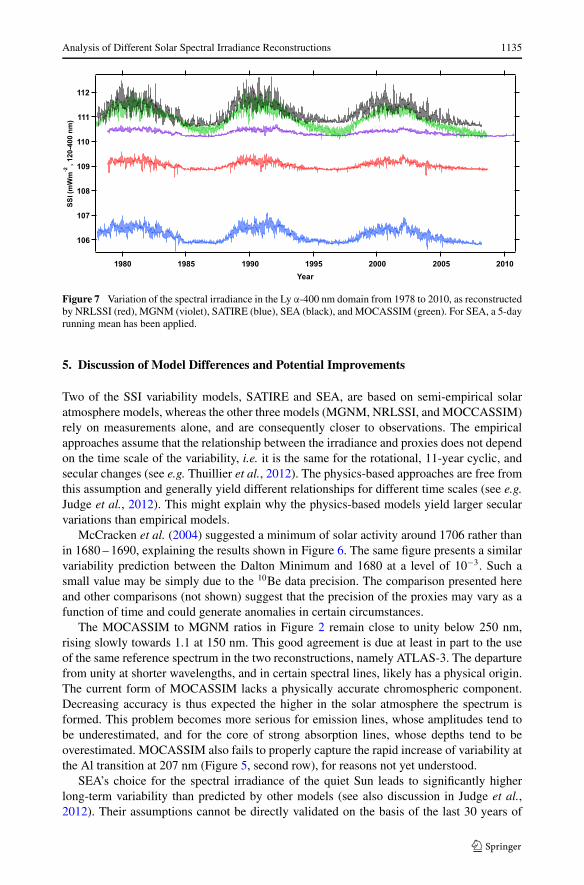
For the 1978 – 2010 period, we have available measurements and proxies, the latter likelya having a better accuracy than in the former time. We have calculated the total SSI betweenLy α and 400 nm using the five models. All models have a daily sampling; however, SEAgiven its method of reconstruction is basically annual. In SEA the 11-year variability iscalculated by scaling the surface areas of the active components with the sunspot number.This relationship works well for the annual data but becomes noisy on shorter time scales. Toallow the homogeneous comparison between different reconstructions, the SEA data werealso shown with daily resolution (after a 5-day running mean smoothing). Some noise in thedata can be explained by the shortcoming outlined above. The results are shown in Figure 7and we note the following: The five predicted variations are in phase. The amplitude isclose to one W m−2 for MOCASSIM, slightly smaller for SEA, close to half a W m−2 forNRLSSI and SATIRE, and a quarter of a W m−2 for MGNM. The use of the Mg II indexgenerates a virtual absence of variability above 300 nm; as the power in the range 300 –400 nm is about six times larger than the power in the range 200 – 300 nm, where SSIvariability exists, the SSI variability in the range 200 – 400 nm is consequently significantlydamped. Absolute mean irradiance spans from 106.5 to 111.5 W m−2 across the five modelswith the best agreement between SEA and MOCASSIM. These absolute values are close butnot identical likely due to the original used spectra. However, the peak-to-peak difference isjust 5 %, which is a value compatible with the reference spectra used by each reconstruction.This will be discussed with some details in Section 5.

The amplitude of the 11-year variability in the 120 – 400 nm band is the largest in MO-CASSIM and the SEA model, and the smallest in the MGNM model. In this interval theSATIRE model predicts larger variability than NRLSSI. However, the variability in the vis-ible part of the spectrum characterizing NRLSSI is larger than that of SATIRE.


Figure 7 Variation of the spectral irradiance in the Ly α-400 nm domain from 1978 to 2010, as reconstructedby NRLSSI (red), MGNM (violet), SATIRE (blue), SEA (black), and MOCASSIM (green). For SEA, a 5-dayrunning mean has been applied.

5. Discussion of Model Differences and Potential Improvements

Two of the SSI variability models, SATIRE and SEA, are based on semi-empirical solaratmosphere models, whereas the other three models (MGNM, NRLSSI, and MOCCASSIM)rely on measurements alone, and are consequently closer to observations. The empiricalapproaches assume that the relationship between the irradiance and proxies does not dependon the time scale of the variability, i.e. it is the same for the rotational, 11-year cyclic, andsecular changes (see e.g. Thuillier et al., 2012). The physics-based approaches are free fromthis assumption and generally yield different relationships for different time scales (see e.g.Judge et al., 2012). This might explain why the physics-based models yield larger secularvariations than empirical models.

McCracken et al. (2004) suggested a minimum of solar activity around 1706 rather thanin 1680 – 1690, explaining the results shown in Figure 6. The same figure presents a similarvariability prediction between the Dalton Minimum and 1680 at a level of 10−3. Such asmall value may be simply due to the 10Be data precision. The comparison presented hereand other comparisons (not shown) suggest that the precision of the proxies may vary as afunction of time and could generate anomalies in certain circumstances.

The MOCASSIM to MGNM ratios in Figure 2 remain close to unity below 250 nm,rising slowly towards 1.1 at 150 nm. This good agreement is due at least in part to the useof the same reference spectrum in the two reconstructions, namely ATLAS-3. The departurefrom unity at shorter wavelengths, and in certain spectral lines, likely has a physical origin.The current form of MOCASSIM lacks a physically accurate chromospheric component.Decreasing accuracy is thus expected the higher in the solar atmosphere the spectrum isformed. This problem becomes more serious for emission lines, whose amplitudes tend tobe underestimated, and for the core of strong absorption lines, whose depths tend to beoverestimated. MOCASSIM also fails to properly capture the rapid increase of variability atthe Al transition at 207 nm (Figure 5, second row), for reasons not yet understood.

SEA’s choice for the spectral irradiance of the quiet Sun leads to significantly higherlong-term variability than predicted by other models (see also discussion in Judge et al.,2012). Their assumptions cannot be directly validated on the basis of the last 30 years of


solar observations as the changes of the quiet Sun are expected to be very small for this pe-riod according to all models. It is known that small-scale magnetic fields are always presenteven in the quietest regions of the Sun (see e.g., Stenflo, 1982; Trujillo Bueno, Shchukina,and Ascensio Ramos, 2004) and can affect irradiance (Afram et al., 2011). Applying thedifferential Hanle effect technique to C2 lines observed at the Instituto RicercheSOlari Lo-carno (IRSOL), Kleint et al. (2010, 2011) suggested that there could be a small variationof the turbulent field strength (3σ -limit) during the descending phase of the solar activity.The continuation of the program will allow us to clarify the contribution of the quiet solarmagnetism to the solar irradiance and test SEA assumption. Furthermore, the discussion interms of absolute values has to take into account different values of the TSI for spectra nor-malization, either 1365 W m−2 or 1360 W m−2. However, these two different values havehere a limited incidence (0.36 %).

SEA and SATIRE, which are physics-based models, both predict comparable variabilityin the Mg I and Mg II lines, which is probably caused by the (inadequate) LTE treatmentof this line. Furthermore, the strong feature around 340 nm in the SATIRE and SEA re-constructions probably results from uncertainties in parameters of CH, NH, and OH bands,which significantly contribute to the opacity of this spectral region.

MGNM uses neutron-monitor and cosmogenic isotope records to extrapolate the Mg II

index into the past. NRLSSI also employs Mg II, and also, solar images and Ca II index.A common feature in these two reconstructions is a measured spectrum to which variabilityis applied based on specific proxies. Furthermore, NRLSSI incorporates a modest varyingbackground component based on simulations of the long-term evolution of magnetic fluxon the solar surface using a flux transport model (Wang, Lean, and Sheeley, 2005). Con-sequently, the NRLSSI and MGNM models employ distinctly independent techniques toestimate past SSI changes so their relatively good agreement prior to the modern era per-haps affords a level of mutual validation.

6. Impacts of the Different SSI Reconstruction on the Radiative Energy Balanceof the Middle Atmosphere

The following analyses are focused on the impact of adopting one specific SSI reconstruc-tions presented above on solar heating rates in the Earth’s middle atmosphere (15 – 80 km).Our choice of the middle atmosphere as a region where the different SSI reconstructions aretested is mainly justified by the two facts: i) the thermal regime of the middle atmosphereis to a large extent determined by the balance between the incoming solar and outgoing in-frared radiation, which makes this region more sensitive to the solar irradiance variations;and ii) the solar heating rates there are much more dependent on SSI variations than they arein the troposphere, where solar heating primary depends on the TSI values (e.g., Semeniuket al., 2011). Due to the large computational complexity of line-by-line radiative transfercodes, atmospheric and climate models normally employ parameterizations or approxima-tions. Our approach in this paper is to calculate the solar heating rates in eight specificspectral bands (Table 3). The advantages as well as the limitations of this approach arediscussed in more detail in the Chemistry-Climate Model Validation Report (CCMVal) ofSPARC (Fomichev et al., 2010; also see Forster et al., 2011), where different approaches arecompared and as a result it is shown that a reasonable compromise is the adoption of eightbands between 121 and 301 nm (Table 3). The inclusion of this method into a full CCMmodel, together with the adoption of variable SSI and its impact, is described in Semeniuket al. (2011).


Our approach is built on the previous analysis presented in the SPARC CCMVal report,where sensitivity of different radiation codes and models to the solar variability (11-yearcycle) is studied using the SSI reconstruction of Lean et al. (2005). The study is restrictedto differences between solar maximum and minimum conditions. The largest response isobserved in the stratopause region (Figure 3.17 in the report) with global mean heating ratechanges of about 0.12 K day−1 in the line-by-line radiation code (Mayer and Kylling, 2005).The adoption of a radiation code using the eight spectral bands of Table 3, covering the 121 –305 nm spectral range, is shown to reproduce very well the results obtained with a line-by-line code. The CCMVal experiment also clearly demonstrates that models, which do notspectrally resolve irradiance in their radiation scheme cannot properly describe variabilitywithin the solar cycle.

In what follows, we use the offline radiation code described in Semeniuk et al. (2011) toestimate the difference in the solar heating rates, which arises from using the different SSIreconstructions (Table 2). The eight bands listed in Table 3 are adopted. The main contri-bution to the solar heating in the middle atmosphere is provided by absorption of ozone, atwavelengths ≈200 – 300 nm, and molecular oxygen in the Schumann–Runge bands (175 –205 nm) and continuum (125 – 175 nm) and in the Ly α line (121 nm) (e.g., Fomichev, 2009).The ozone profile used in our calculations is held constant, and therefore the effects of solarinduced changes in ozone concentration are not taken into consideration. The calculationsare made for a cloudless equatorial atmosphere assuming an overhead Sun and 24-h illumi-nation. Since our focus is on the differences in solar heating rates induced by the choice ofa given SSI reconstruction, the results are discussed in terms of relative values.

The year of 1680 is used as representative of the Maunder Minimum. Year 2008 is chosenas representative of modern time, defined here as the period for which space data are avail-able, and for being considered within the science community as the lowest solar activity forwhich space measurements are available. The year 1781 is chosen as representative of thepast solar maximum, and the year 2002 as representative of solar maximum in modern times.Note that the in the distant past, reconstructed SSI values used here represent annual aver-ages, while modern time values represent daily reconstructions. A caveat is the possibility ofstrong short time variability in the SSI (e.g., the 27-day solar rotational modulation) that canmask the estimation of 11-year or longer cycles. We note that the days chosen for this studyare representative of average conditions. Furthermore, the 27-day rotational modulation isvery weak for solar minimum conditions, in particular for 2008.

Figure 8 shows the differences in solar heating rate values calculated for each recon-struction, relative to the values obtained using the MGNM. Therefore, this figure illustratesthe impact of the different reconstructions for a given year. Note that the SSI values forthe SEA reconstruction at wavelengths below 160 nm, and for MOCASSIM at wavelengthsbelow 150 nm, are assumed to be zero as these reconstructions do not provide values inthose wavelength domains. We also run an experiment where SEA and MOCASSIM seriesare completed using MGNM values, which confirm that, as expected, the larger impact oflower wavelengths is at altitudes above about 60 km. Therefore, in this figure the heatingrates calculated using SEA and MOCASSIM reconstructions are shown only up to 60 kmaltitude.

Figure 9 shows the differences between solar maximum and solar minimum, in modernand past times, for each individual reconstruction. This highlights the differences in solarheating rate values for each selected year from the 2008 values. Once again, the SSI valuesfor SEA at wavelengths below 160 nm and for MOCASSIM at wavelengths below 150 nmare assumed to be zero as they are not available for this study.


Figure 8 Differences in solar heating rate values calculated for each reconstruction relative to the valuesobtained using the MGNM. SSI for SEA at wavelengths below 160 nm and for MOCASSIM at wavelengthsbelow 150 nm, are assumed to be zero as they are not provided. A cloudless condition, overhead Sun, andequatorial ozone profile are considered in calculating the solar heating rates.

Both figures show that the differences are more pronounced in two altitude regions:around 45 km altitude and above 70 km. Around 45 km, the differences among the re-constructions for a given year can be larger than 3 K day−1 (Figure 8). Another importantpoint to note is that the differences are not significantly dependent on solar activity (hereexpressed in terms of solar minimum or maximum). Although SEA results would suggestlarger differences from MGNM for the Maunder Minimum (year 1680), in general thereis no significant difference when comparing reconstructions relative to each other for thepast or current times. For altitudes above about 70 km, where the strong absorption bymolecular oxygen occurs, SEA and MOCASSIM reconstructions completed with zeros forshorter wavelengths result in relatively large heating rate values. However, when both SEAand MOCASSIM reconstructions are completed with the MGNM SSI values at the shorterwavelengths, the heating rate values converge in the mesosphere (not shown). This resultdemonstrates the importance for models to include absorption in the Schumann–Runge con-tinuum and Ly α in order to properly estimate the energy balance at the mesospheric heights.

Different SSI reconstructions lead to different variability from solar maximum to the2008 solar minimum (Figure 9). Again, we observe larger differences in the upper strato-sphere – lower mesosphere, or around 45 km altitude. The amplitude of this variability variesfrom one reconstruction to another, with the SEA reconstruction providing the strongest sig-nal. The year of 1957 stands out as a stronger solar maximum. It is noteworthy that the SEAreconstruction does not capture 2008 as the lowest solar minimum of the modern times.


Figure 9 Differences in solar heating rate values for each selected year (solar maximum years are drawn asthicker lines) with respect to the 2008 values. SSI for SEA at wavelengths below 160 nm and for MOCASSIMat wavelengths below 150 nm are assumed to be zero as they are not provided. A cloudless condition, overheadSun, and equatorial ozone profile are considered in calculating the solar heating rates.

7. Conclusions

Properties of five independent SSI reconstructions are compared to quantify differences intheir absolute values and variability on multiple time scales. The five different reconstruc-tions employ different model formulations and are based on different solar proxies and ob-servational databases. There is a general consensus among the models’ variability and ab-solute values in recent times. However, differences among models tend to increase towardsthe past and in shorter wavelength regions. Solar spectral irradiance and variability recon-structed by NRLSSI and MGNM are consistent at the 5 % level and both are consistentwith MOCASSIM at the 10 % level. Considering that the absolute accuracy of the referencespectra used in these reconstructions is of the order of 3 %, this level of agreement is sat-isfactory. Furthermore, agreement between models increases above 200 nm and for recentperiods.

Divergences do exist across all reconstructions, which require further investigations:

i) Most reconstructions are divergent in terms of both depths and ratios of the Mg I

(285 nm) and Mg II (280 nm) absorption lines. The NRLSSI and MGNM are in bestagreement with observations, but this is expected since both reconstructions are basedin part on the Mg II index.

ii) The 340 – 350 nm wavelength domain, as reconstructed by the SATIRE and SEA mod-els, and the 280 – 320 nm wavelength domain reconstructed by SATIRE, show devia-


tions at the 20 % level with respect to the other reconstructions, at all epochs comparedin this work, and with measured spectra.

iii) At wavelengths below 150 nm, the three available reconstructions (SATIRE, MGNM,and NRLSSI) show deviations with respect to measured spectra at the 10 – 20 % level.For SATIRE, a significant improvement was recently made (Ball et al., 2013).

iv) At wavelengths below 250 nm and epochs prior to 1950, the spectral irradiance of theSEA model is systematically lower compared to other reconstructions, especially whensolar activity is very low.

v) Disagreement among reconstructions depends on time and spectral domains. Averagingover broad spectral domains minimizes these differences.

vi) Even though uncertainties on individual reconstructions presumably become large inthe distant past, most reconstructions yield levels of variability that are consistent within15 %. This can be interpreted as a form of global error estimate on reconstructed vari-ability.

All five SSI reconstructions yield a variability in the 200 – 310 nm wavelength range smallerthan that measured by the SORCE instruments from April 2004 to November 2007. Theclosest predictions are given by MOCASSIM, SATIRE, and SEA (0.10 versus 0.16 W m−2).The two lowest changes are predicted by NRLSSI and MGNM (0.07 and 0.05 W m−2, re-spectively. In the 310 – 400 nm wavelength range, all models yield a reconstructed variabilitythat falls well below that measured by SORCE for this time period. The largest SSI variabil-ity is reconstructed by MOCASSIM, but is still a factor of two less than SORCE reports inthis wavelength range. At the other extreme, the NRLSSI and MGNM reconstructions are,respectively, a factor of 7 and 20 lower than SORCE. The situation is even more discrepantin the 400 – 650 nm range, where SORCE predicts a variability of sign opposite to and mag-nitude larger by a factor of 3 than the NRLSSI, SATIRE, and SEA reconstructions. Finally,none of the models reproduce the SORCE/SIM variability in this recent period.

Our analysis in terms of the solar heating response to the different SSI reconstructionsresults in two primary conclusions. First, the differences in solar heating rates calculated us-ing different reconstructions are often larger than the amplitude of SSI variability during the11-year solar activity cycle, or even between the Maunder Minimum and the modern times,as calculated using a given reconstruction. Second, climate and atmospheric models that donot extend in altitude above the stratosphere do not capture the strong solar signal abovethe stratopause and, hence, do not properly determine the atmosphere’s radiative balancenor, therefore, its dynamical structure. Due to the feedback mechanisms (coupling amongdynamics, radiation, and chemistry), it is unlikely that such models could properly capturethe solar signal in ozone and temperature even at lower altitudes. In addition to identifyingand discussing the uncertainties inherent to SSI reconstructions, the results reported abovemay guide the choice of reconstruction most appropriate for a given research objective. Forexample, if the goal is to capture the solar signal in the upper atmosphere, one needs tochoose a reconstruction that provides reliable values at lower wavelengths.

The quantitative comparisons carried out in this paper will hopefully motivate the devel-opers of SSI reconstructions to consider possible further improvements. It has not been ouraim to declare one reconstruction superior to another. Instead, we attempted to explicitlyidentify differences among the five reconstructions of solar spectral irradiance used in thispaper so as to help climate and atmospheric users to better understand the implications ofchoosing a given reconstruction

Acknowledgements This investigation is supported by the Centre National de la Recherche Scientifique(F), Centre National d’Etudes Spatiales (F), the Federal Office for Scientific, Technical and Cultural Af-


fairs (B). The participating institutes are LATMOS-CNRS (F) (formerly Service d’Aéronomie), Depart-ment of Physics of the University of Toronto (Ca), Canadian Space Agency, Institut für Sonnensystem-forschung of Max-Planck (G), Départment de Physique of Université de Montréal (Ca), York University (Ca),Physikalisch-Meteorologisches Observatorium Davos-World Radiation Center (Ch), Institut d’AéronomieSpatiale de Belgique. J. Lean acknowledges NASA support. A. Shapiro is supported by the Swiss NationalScience Foundation under grant CRSI122-130642 (FUPSOL). C. Bolduc and P. Charbonneau acknowledgesupport from FQRNT-Québec (Team grant 119078). W. Schmutz acknowledges support from Swiss COSToffice (grant nr. C11.0135). A. Shapiro, N. Krivova, W. Schmutz participate in the COST action ES 1005(TOSCA) and profit from the COST meetings. This article is a contribution to the SOLID investigation.

References

Afram, N., Unruh, Y.C., Solanki, S.K., Schüssler, M., Lagg, A., Vögler, A.: 2011, Astron. Astrophys. 526,A120.

Ball, W.T., Unruh, Y.C., Krivova, N.A., Solanki, S.K., Wenzler, T., Mortlock, D.J., Jaffe, A.H.: 2012, Astron.Astrophys. 541, A27.

Ball, W.T., Krivova, N.A., Unruh, Y.C., Haigh, J.D., Solanki, S.K.: 2013, J. Atmos. Sci. submitted.Bolduc, C., Charbonneau, P., Dumoulin, V., Bourqui, M.S., Crouch, A.D.: 2012, Solar Phys. 279, 383.Bolduc, C., Charbonneau, P., Barnabé, R., Bourqui, M.S.A.: 2013, Reconstruction of ultraviolet spectral

irradianceduring the Maunder minimum. Solar Phys. submitted.Crouch, A.D., Charbonneau, P., Beaubien, G., Paquin-Ricard, D.: 2008, Astrophys. J. 677, 723.DeLand, M.T., Cebula, R.P.: 2012, J. Atmos. Solar-Terr. Phys. 77, 225.Egorova, T., Rozanov, E., Manzini, E., Haberreiter, M., Schmutz, W., Zubov, V., Peter, T.: 2004, Geophys.

Res. Lett. 31, L06119.Fomichev, V.I.: 2009, J. Atmos. Solar-Terr. Phys. 71, 1577.Fomichev, V.I., Forster, P.M., Cagnazzo, C., Johnsson, A.I., Langematz, U., Rozanov, E., et al.: 2010, In:

Eyring, V., Shepherd, T.G., Waugh, D.W. (eds.) Chemistry-Climate Model Validation, SPARC Rep. 5.Chapter 3.

Fontenla, J., White, O.R., Fox, P.A., Avrett, E.H., Kurucz, R.L.: 1999, Astrophys. J. 518, 480.Forster, P.M., Fomichev, V.I., Rozanov, E., Cagnazzo, C., Jonsson, A.I., Langematz, U., et al.: 2011, J. Geo-

phys. Res. 116, D10302.Fröhlich, C.: 2012, Surv. Geophys. 33, 453.Haberreiter, M., Schmutz, W., Hubeny, I.: 2008, Astron. Astrophys. 492, 833.Harder, J.W., Fontenla, J.M., Pilewskie, P., Richard, E.C., Woods, T.N.: 2009, Geophys. Res. Lett. 36(7),

L07801. doi:10.1029/2008GL036797.Haigh, J.D., Winning, A., Toumi, R., Harder, J.W.: 2010, Nature 467, 696.Harder, J.W., Fontenla, J., Lawrence, G., Woods, T.N., Rottman, G.: 2005b, Solar Phys. 203, 169.Harder, J.W., Lawrence, G., Fontenla, J., Rottman, G., Woods, T.N.: 2005a, Solar Phys. 203, 141.Harder, J.W., Thuillier, G., Richard, E.C., Brown, S.W., Lykke, K.R., Snow, M., McClintock, W.E., Fontenla,

J.M., Woods, T.N., Pilewskie, P.: 2010, Solar Phys. 263, 3.Ineson, S., Scaife, A.A., Knight, J.R., Manners, J.C., Dunstone, N.J., Gray, L.J., Haigh, J.D.: 2011, Nat.

Geosci. 4, 753.Jiang, J., Cameron, R.H., Schmitt, D., Schüssler, M.: 2011, Astron. Astrophys. 528, A82.Judge, P., Lockwood, G.W., Radick, R.R., Henry, G.W., Shapiro, A.I., Schmutz, W., Lindsey, C.: 2012,

Astron. Astrophys. 544, A88.Kleint, L., Berdyugina, S.V., Shapiro, A.I., Bianda, M.: 2010, Astron. Astrophys. 524, A37.Kleint, L., Shapiro, A.I., Berdyugina, S.V., Bianda, M.: 2011, Astron. Astrophys. 536, 47.Kopp, G., Lean, J.L.: 2011, Geophys. Res. Lett. 38, L01706.Krivova, N.A., Balmaceda, L., Solanki, S.K.: 2007, Astron. Astrophys. 467, 335.Krivova, N.A., Solanki, S.K., Floyd, L.: 2006, Astron. Astrophys. 452, 631.Krivova, N.A., Solanki, S.K., Unruh, Y.C.: 2011, J. Atmos. Solar-Terr. Phys. 73, 223.Krivova, N.A., Vieira, L.E.A., Solanki, S.K.: 2010, J. Geophys. Res. 115, A12112.Krivova, N.A., Solanki, S.K., Fligge, M., Unruh, Y.C.: 2003, Astron. Astrophys. 399, L1.Kurucz, R.L.: 1991, In: Cox, A.N., Livingston, W.C., Matthews, M.S. (eds.) Solar Interior and Atmosphere,

The University of Arizona Press, Tucson, 663.Kurucz, R.L.: 1993, ATLAS9 Stellar Atmosphere Programs and 2 km/s Grid, CD-ROM No. 13, Smithsonian

Astrophysical Observatory, Cambridge.Lean, J.: 2000, Geophys. Res. Lett. 27, 2425.Lean, J.L., DeLand, M.T.: 2012, J. Climate 25, 2555.

http://dx.doi.org/10.1029/2008GL036797


Lean, J.L., Rottman, G.J., Kyle, H.L., Woods, T.N., Hickey, J.R., Puga, L.C.: 1997, J. Geophys. Res. 102,29939.

Lean, J., Rottman, G., Harder, J., Kopp, G.: 2005, Solar Phys. 230, 27.Mayer, B., Kylling, A.: 2005, Atmos. Chem. Phys. 5, 1855.McCracken, K.G., McDonald, F.B., Beer, J., Raisbeck, G., Yiou, F.: 2004, J. Geophys. Res. 109, 12103.Merkel, A.W., Harder, J.W., Marsh, D.R., Smith, A.K., Fontenla, J.M., Woods, T.N.: 2011, Geophys. Res.

Lett. 38, L13802.Oberländer, S., Langematz, U., Matthes, K., Kunze, M., Kubin, A., Harder, J., Krivova, N.A., Solanki, S.K.,

Pagaran, J., Weber, M.: 2012, Geophys. Res. Lett. 39, L01801.Rottman, G.: 2000, Space Sci. Rev. 94, 83.Rottman, G.J.: 2005, Solar Phys. 230, 7.Schmidt, G.A., Jungclaus, J.H., Ammann, C.M., Bard, E., Braconnot, P., Crowley, T.J., et al.: 2012, Geosci.

Model Dev. 5, 185.Semeniuk, K., Fomichev, V.I., McConnell, J.C., Fu, C., Melo, S.M.L., Usoskin, I.G.: 2011, Atmos. Chem.

Phys. 11, 5045.Shapiro, A.I., Schmutz, W., Schoell, M., Haberreiter, M., Rozanov, E.: 2010, Astron. Astrophys. 517, A48.Shapiro, A.V., Rozanov, E., Egorova, T., Shapiro, A.I., Peter, T., Schmutz, W.: 2011b, J. Atmos. Solar-Terr.

Phys. 73, 348.Shapiro, A.I., Schmutz, W., Rozanov, E., et al.: 2011a, Astron. Astrophys. 529, A67.Shapiro, A.V., Rozanov, E.V., Shapiro, A.I., Egorova, T.A., Harder, J., Weber, M., Smith, A.K., Schmutz, W.,

Peter, T.: 2013, J. Geophys. Res. doi:10.1002/jgrd.50208.Snow, M., McClintock, W.E., Woods, T.N., Rottman, G.: 2005, Solar Phys. 230, 295.Solanki, S.K., Schüssler, M., Fligge, M.: 2002, Astron. Astrophys. 383, 706.Solanki, S.K., Unruh, Y.C.: 1998, Astron. Astrophys. 329, 747.Solanki, S.K., Usoskin, I.G., Kromer, B., Schüssler, M., Beer, J.: 2004, Nature 431, 1084.Solomon, S.D., Qin, D., Manning, M., Chen, Z., Marquis, M., Averyt, K.B., Tignor, M., Miller, H.: 2007,

Climate Change 2007, The Physical Science Basis (Contribution of Working Group I to the FourthAssessment Report of the Intergovernmental Panel on Climate Change), Cambridge University Press,Cambridge, 188.

Stenflo, J.O.: 1982, Solar Phys. 80, 209.Tapping, K., Boteler, D., Charbonneau, P., Crouch, A., Manson, A., Paquette, H.: 2007, Solar Phys. 246, 309.Thuillier, G., Hersé, M., Simon, P.C., Labs, D., Mandel, H., Gillotay, D., Foujols, T.: 1998, Solar Phys. 177,

41.Thuillier, G., Floyd, L., Woods, T.N., Cebula, R., Hilsenrath, E., Hersé, M., Labs, D.: 2004, In: Pap, J., Fox,

P. (eds.) Solar Variability and Its Effect on Climate, AGU Geophys. Monogr. 141, 171.Thuillier, G., DeLand, M., Shapiro, A., Schmutz, W., Bolsée, D., Melo, S.M.L.: 2012, Solar Phys.

doi:10.1007/s11207-011-9912-5.Trujillo Bueno, J., Shchukina, N., Ascensio Ramos, A.: 2004, Nature 430, 326.Unruh, Y.C., Ball, W.T., Krivova, N.A.: 2012, Surv. Geophys. 33, 475.Unruh, Y.C., Solanki, S.K., Fligge, M.: 1999, Astron. Astrophys. 345, 635.Vieira, L.E.A., Solanki, S.K., Krivova, N.A., Usoskin, I.: 2011, Astron. Astrophys. 531, A6.Wang, Y.-M., Lean, J.L., Sheeley, N.R. Jr.: 2005, Astrophys. J. 625, 522.Wenzler, T., Solanki, S.K., Krivova, N.A., Fröhlich, C.: 2006, Astron. Astrophys. 460, 583.Woods, T.N., Chamberlin, Ph.C., Harder, J.W., Hock, R.A., Snow, M., Eparvier, F.G., Fontenla, J., McClin-

tock, W.E., Richard, E.C.: 2009, Geophys. Res. Lett. 36, L01101.

http://dx.doi.org/10.1002/jgrd.50208

http://dx.doi.org/10.1007/s11207-011-9912-5

analysis of different solar spectral irradiance reconstructions and their impact on solar heating...

Documents