analysis of crime in chicago: new perspectives to an old...
TRANSCRIPT

Analysis of crime in Chicago: new perspectives to an old question using spatial panel econometrics
Benoît DELBECQ
Food and Agricultural Policy Research Institute
University of Missouri
Columbia, Missouri, Etats-Unis
Rachel GUILLAIN
Laboratoire d’Economie et de Gestion
Université de Bourgogne
BP 26611
21066 Dijon Cedex, France
Diègo LEGROS
Laboratoire d’Economie et de Gestion
Université de Bourgogne
BP 26611
21066 Dijon Cedex, France
Keywords: City of Chicago, fixed and random effects, social disorganization theory, spatial econometrics, violent crime.
Classification JEL : C23, D01, R23
1
- 1 - Introduction
Chicago has been historically infamous for being the murder capital of America since the days of organized crime during the prohibition. Furthermore, the combination of its rapid urbanization and its socio-economic heterogeneity makes it an ideal case for the study of linkages between urbanism and crime. The Chicago School of Sociology is rich in developments and teachings on the subject and has largely inspired analyses conducted in the fields of economics and sociology.
Since the 90s, the City of Chicago has been conducting a series of crime prevention policies. These policies appear to have been successful since Chicago dropped out of the top 25 most dangerous cities in the U.S. in 2006. Nevertheless, the number of murders per inhabitant remains higher than in New York City or Los Angeles and the recent hike in crimes committed in Chicago puts the current crime-fighting policies into question. Moreover, public policies are challenged with the economic crisis and the control of spending compared to the efficiency is one major concern of decision-makers.
In this context, the objective of this paper is to identify the determinants of violent crime in the city of Chicago over the 2009-2011 period. More specifically, we analyze the consequences of inequalities over violent crime. We rely on the social disorganization theory (Shaw and McKay, 1942). Criminal activities are rooted in a lack or a weakening of social control exerted by communities because of poverty, residential instability and racial/ethnic heterogeneity. To do so, we use spatial panel econometrics tools developed by Elhorst (2012). These estimation techniques allow the joint treatment of the spatial and temporal dimensions which are inherent to the phenomenon of urban crime.
The second section is devoted to the presentation of the disorganization theory. Data, weight matrix and method of estimation are presented in the third section. The fourth section is dedicated to the results.
- 2 - Disorganization theory and crime
Our empirical analysis is based on the theory of social disorganization, which itself was born out of the ecological theories developed by Shaw and McKay (1942). In urban areas, delinquency is not randomly distributed in space but tends to be concentrated in poor and socially excluded places. These basic principles of disorganization theory were developed early but recognition and success did not happened until the 80s.
Generally speaking, individuals are subject to neighborhood effects. The place where an individual lives has consequences on the opportunities he can get. When choosing a residence, proximity to positive amenities such as reputable schools is an important criterion to guarantee a good quality education. Similarly, peer group effects and role models play a major role in urban segregation. Opportunities to get a job are higher when an individual is surrounded by people who have a job because of the social pressure to find a job. Similarly, young people are prone to imitate the behavior of older members of their family or their community. In other words, individuals generate positive or negative spillovers (Arnott and Rowse, 1987; Benabou, 1993; Glaeser et al., 1996; Selod and Zénou, 2006).
Similar mechanisms are identified as determinants of crime. The structural characteristics of an area are sources of differentiated levels of crime, so that a geography of

2
crime is observed. More precisely, the social disorganization theory is defined by Sampson and Groves (1989) as “an inability of a community structure to realize the common values of its residents and maintain effective social controls”. This theory posits that social and economic difficulties, residential mobility, and ethnic heterogeneity hinder the emergence of social links (Veysey and Messner, 1999). They favor the development of violent or antisocial behaviors. Indeed, economic, demographic and social characteristics of a neighborhood have consequences on the social links that sustain the “collective efficacy” (Sampson et al., 1997). Common social relations and values shared by a community are crucial for establishing rules of good behavior. Institutions or organizations such as family, school, and religion must exert their positive influence through the supervision of adults, references to models of good behavior and the transmission of rules of respect and sharing. On the one hand, a community with a strong collective efficacy is more likely to maintain order and social organization is then a way to fight crime. On the other hand, social disorganization takes over when formal and informal linkages and networks are not easily established because of a malaise in the community. This phenomenon worsens with residential instability because development and establishment of collective efficacy is a slow process. Furthermore, racial and/or ethnic heterogeneity between residents also favors the emergence of deviant behaviors because social isolation does not foster the emergence of behavior controls. As a consequence, socio-economic characteristics observed in a location are only part of the story when explaining crime. Peer effects between individuals create a phenomenon of contagion named ‘social multiplier’ by Glaser et al. (2003).
These theoretical developments have been empirically tested primarily in American and Canadian cities, likely because of data availability. Violent crimes are well explained by the social disorganization theory (Kelly, 2000). Several empirical studies have been done successfully in this context for the city of Chicago (see, among others, Browning at al., 2004; Browning, 2009; Morenoff et al., 2001; Sampson et al., 1997; Shaw and McKay, 1942; Vélez and Richardson, 2011; Wang, 2005; Wang and Arnold, 2008; Wilson, 1987). While caution is warranted when making comparisons because of differences in data and techniques, findings seem to indicate that social-economic conditions have more influence on criminality than ethnic/racial heterogeneity and residential instability. Moreover, spatial effects are highlighted as playing an important role in crime.
- 3 - Methodology
To the best of our knowledge, empirical studies on Chicago do not rely on data after the 2008 subprime crisis after which crime, and especially violent crime, has been trending up. In this section, we first outline the importance of time and space when studying crime. Second, we present data and weight matrix, and third, we describe the estimation techniques.
3.1 Time and space If Anselin (1988) stresses the importance of space in crime, Buananno et al. (2011)
notice that space is not systematically integrated in empirical analyses of crime. Nevertheless, a couple of arguments lead to consider it systematically.
The first argument relies on the artificial character of frontiers. Census tracts are subdivisions of counties constructed to collect data. They are originally defined to be as homogeneous as possible based on demographic and socio-economic characteristics and to be

3
stable over time. Census tracts vary in size because of differences in population density. This is not specific to crime but it has to be taken into account: a boundary could separate artificially an area. Moreover, since the variables characterizing disorganization theory tend to cluster in space, it is not possible to consider spatial areas as independent.
The second argument refers to the interactions that lead to crime. Census tracts are interdependent because diffusion, amplification, and exposure processes are present in crime. In a spatial unit, contextual factors influence the probability of becoming a criminal and studies show that crime is mainly committed near the place of residence of the criminal. However, criminal activities are not necessarily committed within administrative boundaries. Moreover, corridors of violence tend to appear over time as criminal activities in a location induce crime in spatially connected locations, this phenomenon not being specific to gang-related crime (Cohen and Tita, 1999; Messner et al., 1999; Morenoff and Sampson, 1997; Morenoff et al., 2001; Rosenfled et al., 1999; Smith et al., 2000; Tita and Radil, 2011; Wand and Arnold). Therefore, there exists a spatial dependence with respect to crime between spatial units.
This spatial dimension is associated to a temporal dimension so that we use spatial panel econometrics tools.
3.2 Data and weight matrix Data used to measure criminal activity are collected from the City of Chicago Data
Portal website where the city has been publishing geo-localized data on crime since 2001. They are recorded by the CLEAR system (Citizen Law Enforcement Analysis and Reporting) of the Chicago Police Department. We focus on violent crime because they are known to be well reported and because they are well explained by the theory of social disorganization (Andresen, 2006; Kelly, 2000; Morenoff et al., 2001; Vélez and Richardson, 2012; Wand, 2005; Wang and Arnold, 2008). There is no absolute definition of violent crime but the following are the most frequently used categories in the literature: first degree murder, aggravated robbery, aggravated assault, criminal sexual assault, kidnapping, and arson. Since each crime is precisely located by latitude and longitude, the Chicago crime data can be aggregated at any spatial scale. The demographic and socio-economic data used to explain crime are collected from the Census Bureau. Certain variables of interest are only available through the 5-year estimates of the American Community Survey (ACS) for which the smallest spatial unit is the census tract. Therefore, we choose the census tract as our scale of analysis. At the time of this analysis, only three years of 5-year ACS estimates are available: 2009, 2010, and 2011. Over this time period, 53,934 violent crimes were reported in Chicago. We build our dependent variable by taking the log of the number of violent crimes per inhabitant in each census tract of the City of Chicago for each year of the 2009-2011 period. After eliminating the tracts with a zero population, such as the Chicago O’Hare airport and some large green spaces, we are left with 761 census tracts. The boundaries of some census tracts were changed for the 2010 Census, so we used Logan et al.’s (2013) methodology to adapt the 2009 to the new limits.
Data used to represent social disorganization theory vary from a study to the other one mainly conditioned by their availability (Andresen, 2006; Deane et al., 2008). We faced the same constraints but we select the most widely used variables in empirical studies particularly on Chicago. For the socio-economic dimension, four data are used: median income, number of family living under the poverty level, unemployment, number of people aged of 25-64 years with no high-school diploma. Except for the income, an increasing value of their

4
variable tends to increase the rate of violent crime. Only the variable of vacant residence is available to reflect the residential instability, a factor supposed aggravating crime. Racial and ethnic heterogeneity is approached by the number of Afro-Americans and by the number of Hispanic people. Wang and Arnold (2008) point out that about 70% of the Hispanic community is Americano-Mexican. Heterogeneity is a barrier to the development of social links and controls and is perceived as aggravating crime. All these variables are related to the population of the census tract and are in log.
Two other variables are traditionally added in studies on violent crime: density and the number of young people of 15-24 years old. The expected sign is positive since these factors increase crime.
The spatial weight matrix allows specifying the structure of connectivity between the census tracts in Chicago. Following the literature on the violent crime, we use a contiguity matrix which the value of 1 is the census tracts share a common administrative boundary. The element of the diagonal has the value of 0 and each term is defined as:
1 if the are contiguous0 otherwiseij
census tractsw
=
The choice of the spatial weight matrix is crucial in spatial econometrics. Our choice is based on the literature of crime. Tita and Greenbaum (2009) point out that an abundant literature question the reasons why crime happens at a place rather than another. Crime activities follow logic of low distance. In other terms, a crime committed in a census tract influences the criminal activities occurring in a closed proximity, especially for the violent crime. This justifies the use of a matrix of contiguity (Browning et al., 2004; Browning, 2009; Tita and Radil, 2010).
3.3 Estimation From a theoretical point of view, individual and temporal heterogeneity can be
considered constant or random leading to the models of fixed effects and random effects. Traditionally, when data are related to countries or regions, the model with fixed effects is preferred while the model with random effects is more dedicated to individuals. Besides the individual and/or temporal heterogeneity, neighboring effects have to be considered since crime is a social phenomenon which is not restricted in administrative boundaries. Moreover, the rate of crime in one place could influence the one in another place, so that neglected spatial linkages could bias estimations.
We follow Elhorst’s recommendation (2012) to identify the appropriate model that generates the data. We estimate the following model:
1 1
(optional) (optional)N N
it ij ij it ij ijt i t itj j
y w y x w xδ α β θ µ λ ε= =
= + + + + + +∑ ∑ [1]
ity is the number of criminal activities in the census tract i at the year t with 1,..., ; 1,...,i N t T= = in the general case. In our case, N = 761 and 2009, 2010, 2011t = .
ijw is the i, jth term of the weight matrix W defined previously;δ is the autoregressive parameter; α is the constant; itx is the vector of exogenous parameters; β and θ are vectors of

5
parameters to estimate; iµ designates spatial-specific effects and tλ the time-specific effects;
itε is the error term independently and identically distributed for i and t, with 0 mean and
variance 2σ and ( )'; 0.it itE ε ε =
The first step is to determine the appropriate panel model and the second the appropriate spatial specification.
Following Elhorst (2012), we start by looking for individual effects in our data, namely we want to determine whether the census tracts are homogenous or heterogeneous. To do so, we perform a likelihood ratio (LR) test with the null hypothesis of jointly nullity of individual effects. The LR statistic at 761 degree of freedom equals 3 922.59 (p-value = 0) so that individual effects are not simultaneously null. The same test is performed for the temporal effects: the null hypothesis namely time-period fixed effects are jointly insignificant, must be rejected (LR test with 3 degrees of freedom = 92.62, p-value = 0). These results indicate that the model has to be extended with individual and time-period fixed effects named also a two ways fixed effects model following the terminology of Baltagi (2005). Since the individuals are spatial area (here census tracts), Elhorst (2012) speaks about spatial and time-period fixed effects model. We perform a Hausman test to test the hypothesis of random individual effects or fixed individual effects and the results are in favor of a model of individual fixed effects (Lee and Yu, 2010).
<< Table 1: Violent crime in Chicago: models without spatial dependences >>
For the spatial dependence, we first use the specific to general procedure. We examine the presence of spatial effects in a pooled model, in a spatial-fixed effects model, in a time-period fixed effects and in a spatial and time-period fixed effects because results of the tests can be influenced by the type of effects included. In table 2, results of Lagrange multiplier’s test are reported (standard and robust versions, the routines in panel are provided by Elhorst (2012). Columns 2, 4 and 6 inform us that the hypotheses of no spatially lagged variable and no spatially autocorrelated error term cannot be accepted. For the spatial and time period fixed effect, the results of the tests are in favor of spatial effects in the form of spatial lag model.
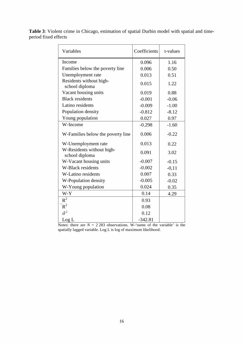
<< Table 2: Spatial autocorrelation test results estimated by OLS >> << Table 3: Violent crime in Chicago, estimation of spatial Durbin model with spatial and time-period fixed effects >>
The general to specific procedure is examined: as pointed out by Elhorst (2012), there is now agreement in the literature regarding the two procedures because each of them has pros and cons. For the general procedure, the question is to determine whether the Durbin model can be reduced to a SAR or SEM model. If the two procedures conclude to a SAR or SEM model, Elhorst (2012) recommends to apply it to the data otherwise the Durbin model is privileged. So a Durbin model is estimated with a bias correction procedure proposed by Lee and Yu (2010c) and extended by Elhorst (2012). Results are reported in table 3. The hypotheses H0 : 0θ = and H0 : 0θ δβ+ = are tested with a Wald statistic and a likelihood ratio test of the spatial common factors. Results (table 4) are not in favor of H0.
<< Table 4: Results of common factor tests (spatial Durbin specification with spatial and time-period fixed effects)>>
At this stage, the procedure leads us to a Durbin model with spatial and temporal fixed effects. Nevertheless, we do not follow the conclusions of the tests. Indeed, in table 1, introduction of individual (spatial) fixed effects explains a great variability of the endogenous

6
variable, which impacts the coefficient of determination. Its value is 62% for the pooled model and drop to 6% when individual (spatial) effects are introduced. When fixed effects are introduced in the temporal dimension only, the percentage of variability explained is the same as the one in the polled model. As a consequence, while the Hausman test is in favor of a model with fixed effect, it seems that model with random effect describes best the data. The conclusion of the Hausman’s test could be explained because it is based (among other) on the distance between the OLS estimator and intra-individual estimator. The difference of the coefficient of the crime measure spatially lagged (0.1448) in the individual (spatial) fixed effects model and in the random model (0.455) could then explain the conclusion of the test.
Since spatial autocorrelation has been detected in the data, we have to identify the appropriate spatial model by examining if the Durbin model can be reduced to a SAR or SEM model. We estimate:
1 1
N N
it ij ij it ij ijt itj j
y w y x w xδ α β θ ε= =
= + + + +∑ ∑ [2]
With the same notations as equation [1]. Results are presented in table 5. Results of the tests (table 6) indicate that the Durbin model remains the best model for the data. The choice of the panel with random effects is reinforced when we examine the value of ϕ parameter. The value is 0.4520 and the parameter is significantly different of zero so that it is in favor of model with random effects according to Baltagi (2008b).
<< Table 5: Violent crime in Chicago, estimation of spatial Durbin model with random effects >> << Table 6: Results of Wald test (estimation of spatial Durbin model with random effects) >>
To sum up, different tests reveal the presence of heterogeneity and spatial autocorrelation that have to be taken into account into in the estimations. Results indicate that fixed effects capture an important variability of crime. This can be due to the small temporal dimension of data or the small spatial scale (census tracts) used. Indeed, changes in characteristics of census tracts could not be perceived from one year to the next. For that reason, a model with random effects is adopted. The test of the common factor concludes in favor of a Durbin model so that we estimate a spatial Durbin model with random effects.
- 4 - Results
Interpreting estimation results from spatial models is not as immediate as with aspatial models when spatial lags of the dependent and/or independent variable(s) are present. As such, special care is required to interpret estimated coefficients. Specifically, a change in the value of an explanatory variable affects not only the spatial unit itself but it also has an indirect effect on the whole spatial system via the spatial multiplier (LeSage, 2008; LeSage and Pace, 2009). Various interpretations can be proposed. It is possible to study the impact of changes in explanatory variables in a spatial unit i on spatial unit i itself or another spatial unit j. This is interesting to investigate shock diffusion phenomena (Dall’erba and Le Gallo, 2008; Le Gallo et al., 2003). We favor an interpretation based on the average effect which is more appropriate in our case because we investigate the impact of structural characteristics of census tracts on crime rate, taking into account dependence effects among census tracts.

7
In this context, three types of effects can be calculated and interpreted (Autant-Bernard and LeSage, 2011; LeSage, 2008; LeSage and Pace, 2009). The average direct effect corresponds to the impact of a change in an explanatory variable in a spatial unit i on the dependent variable in the same spatial unit. Unlike the marginal effects of aspatial linear models, the direct impacts of explanatory variables differ from the estimated coefficients because they include effects emanating from neighboring locations feeding back to spatial unit i. The average indirect impact corresponds to spatial spillovers, that is to say the impact on a spatial unit i of a change in an explanatory variable in all other location or, reciprocally, the impact of a change in an explanatory variable in a spatial unit i on all other locations. The average total effect is the sum of average direct and indirect effects.
Thus, the magnitude and statistical significance of spatial effects cannot be inferred directly from the estimated coefficients on the exogenous variables. Nonetheless, we report these parameters in table 6 because they are useful to perform the specification tests described in the previous section. Coefficient estimates may be negative or even insignificant while the corresponding marginal effects, which include spatial spillovers, are positive (and reciprocally). Therefore, it is necessary to analyze table 7 in which the estimated average direct, indirect, and total effects are reported. Given the complexity of these average marginal effects, statistical inference is conducted using the simulation approach described in Elhorst (2012). This method consists in generating distributions for the parameters of the model by drawing randomly from a multivariate random normal distribution with mean vector and variance covariance matrix the maximum likelihood estimates of the regression coefficients and their variance covariance matrix, respectively. These simulated parameter distributions are used to generate average direct, indirect, and total effects distributions with which we subsequently calculate t-statistics. Given that the data is pooled by year, the temporal dimension does not have any influence and marginal effects are location-specific (LeSage and Pace, 2009). In our case, direct effects capture the impact of a change in the structural variables specific to a census tract on the crime rate in this census tract. Indirect effects represent the spatial diffusion among census tracts, i.e., the aggregate impact on the crime rate of a specific census tract following a change in an explanatory variable in all other census tracts, or symmetrically, the total effect of a change in an explanatory variable in a specific census tract on the crime rate in all other census tracts. Since variables are expressed in logarithmic form, coefficients as well as marginal effects correspond to elasticities (LeSage and Pace, 2009).
<< Table 7: Marginal effects of the spatial Durbin model with random effects >>
Generally speaking, violent crime in Chicago is well explained by our application of the theory of social disorganization. This finding corroborates the results of previous studies conducted on 1990s Chicago crime data using methods that explicitly take the role of space into account (e.g., Browning et al., 2004; Browning, 2009; Morenoff et al., 2001; Velez and Richardson, 2012; Wang, 2005; Wang and Arnold, 2008). However, given that variables and estimation techniques differ, one needs to be cautious when making comparisons. The subprime crisis does not appear to have had an impact on the determinants of crime in the city of Chicago.
Examining the average total effects allows the evaluation of the global impact of the explanatory variables on crime in all census tracts. We observe that socio-economic difficulties influence violent crime positively. Specifically, the income elasticity of crime is negative and significant, whereas elasticities with respect to the number of households living under the poverty threshold, unemployment rate, and the number of people who do not have a high school degree are positive and significant. Similarly, more residential mobility is

8
associated with higher crime rates as indicated by the positive and significant coefficient on the number of vacant properties. Signs and magnitude are in line with what we expected.
The effect of racial and ethnic heterogeneity is less clear-cut. While a larger number of African-Americans tends to be associated with more violent crime, the opposite is true for people of Hispanic ethnicity. Direct and indirect effects have the same signs but the presence of Hispanic people is not associated with a statistically significant average direct effect. This is linked to the way this heterogeneity is captured at the census tract level. As with many empirical studies based on the theory of social disorganization, racial and ethnic heterogeneity is associated with variables related to the number of African-Americans and/or Hispanics in regression models. An important hypothesis is underlying this approach, namely that the presence of African-Americans and/or Hispanics in a spatial unit is a sign of heterogeneity. For instance, Browning et al. (2004) use the number of people of Hispanic ethnicity in Chicago and find a negative effect, which, while unexpected, is in line with other studies (Morenoff et al., 2001; Sampson et al., 1997). In our case, however, the estimated coefficient associated with the Hispanic population is negative, while it is positive for African-Americans. Therefore, it appears delicate to draw any conclusion regarding the role of racial and ethnic heterogeneity on violent crime. The hypothesis underlying the choice of variable has limitations. On these grounds, Kubrin (2000) recommends calculating the relative proportions of all race and ethnic groups to check the effective heterogeneity of each spatial unit. Even so racial and ethnic heterogeneity does not appear linked to crime in Chicago. Velez and Richardson (2012) build a heterogeneity index which ranges from 0 (homogeneity) to 1 (heterogeneity) and find an inverse relationship with the homicide rate per inhabitant. The authors explain that this result is an artifact unique to the city of Chicago. Homogeneous communities tend to be primarily comprised of African-American or Hispanic populations while white mixed neighborhoods are more heterogeneous in nature. As a consequence, we argue that this issue of racial and ethnic heterogeneity requires further investigation, an undertaking that we leave for future research.
The direct effects related to the social disorganization theory variables are significant and have identical signs with the exception of the number of people of Hispanic origin which is not significant. The difference between direct effects and the corresponding estimated coefficients allows us to quantify feedback effects (see Table 8). These feedback effects are not negligible. They are largest for the share of adults with no high school degree (35.71%), and they are 22.5% and 25% of the average direct effect for the variables associated with African-Americans and Hispanic populations, respectively. Feedback effects are at least 8% for the other variables. Thus, impacts in neighboring census tracts which feed back into each census tract via spatial linkages increase the prevalence of violent crime for all variables but income (which lowers it) and the presence of Hispanics (insignificant). From an estimation standpoint, it is crucial to note that limiting oneself to simply interpreting the coefficients underestimates the full impacts of each variable. Besides, it also illustrates the importance to include spatial effects when analyzing crime as recommended by Tita and Greenbaum (2009) and Buaonamo et al. (2011).
<< Table 8: Feedback effects as a proportion of average direct effects >>
The indirect effects, which represent spatial spillovers, are also statistically significant and proportionally larger than the direct effects. Thus, neighborhood effects are important components when explaining violent crime in Chicago. The amplification phenomenon underscored in crime studies is particularly pronounced here.
The presence of men aged 15 to 24 does not have a significant impact on crime. Worral (2004) and Velez and Richardson (2012) identify a significant and positive impact in Los

9
Angeles and Chicago, respectively while Browning et al. (2010) find this variable to be insignificant for the city of Columbus. The influence of this variable could be better captured with data that would allow the establishment of linkages between educational achievements and the presence of a young male population. These data are, however, unavailable.
Population density exhibits negative average direct effects (-0.309) and positive average indirect effects (0.399) of similar absolute magnitudes, which combined leads to slightly positive average total effects. This illustrates the difficulties associated with identifying the impact of population density on crime. A higher density in all census tracts tends to be associated with more violent crime. This illustrates the argument made by Morenoff et al. (2001), namely that while denser cities generally exhibit higher crime rates, this link is less obvious at the intra-urban scale, particularly in Chicago. Because of a larger population, the risk of violent crime increases in dense neighborhoods. However, studies show that the depopulation is often a sign of serious socio-economic difficulties which can lead to low population zones having high crime rates (Browning et al., 2004). In Chicago, low density neighborhoods are hit the hardest by crime, while high density zones generally exhibit low crime rates. This is reflected in the estimated negative direct impact. Interpreting the spillover effects of population density is more difficult and requires further refinements. For instance, population density may reveal the attractive nature of good institutional governance which permits the emergence of a social control. This acts as a protection against crime. However, population density can simply be the result of low land use costs. In this situation, consequences on the establishment of social linkages and crime are different.
- 5 - Conclusion
Generally speaking, social disorganization theory allows identifying determinants of violent crime in Chicago. We provide an analysis that combines spatial and temporal dimension. Nevertheless, further extensions are required: the study period has to be extended and the concept of inequality between individuals has to be specified more accurately.
In terms of public policies, results outlined with the disorganization theory imply social links between individuals have to be developed. Repressive politics are not adequate to reduce crime. This is not in line of Becker’s claim (1968): a crime is committed if the gains are higher than costs, so that fight crime leads to reinforce punishments of crime. There two sides of the crime determinants converge today: crime is an act influenced by the potential penalty and by peer effects. The Chicago’s public policies mix both: penalties are radical but some local initiatives favor the development of social links such as CAPS (Chicago’s Alternative Policing Strategy). The empirical studies of crime would be improved by taking into account the respective effects of the repressive and supportive public policies.

10
References ANDRESEN MA (2006) A spatial analysis of crime in Vancouver, British Columbia: a synthesis of social disorganization and routine activity theory. The Canadian Geographer 50: 487-502.
ANSELIN L (1988) Spatial econometrics: Methods and models. Kluwer Academic Publishers, Dordrecht.
ANSELIN L (2010) Thirty years of spatial econometrics. Papers in Regional Science 89: 3-25.
ANSELIN L, BERA AK, FLORAX R, YOON MJ (1996) Simple Diagnostic tests for spatial dependence. Regional Science and Urban Economics 26:77-104.
ANSELIN L, JAYET H, LE GALLO J (2008) Spatial panel econometrics. In: Matyas L, Sevestre P The Econometrics of Panel Data: Fundamentals and Recent Developments in Theory and Practice. Dordrecht: Springer-Verlag, 625-660.
ARNOTT R, ROWSE J (1987) Peer group effects and educational attainment. Journal of Public Economics 32: 287-305.
AUTANT-BERNARD C, LESAGE J (2011) Quantifying knowledge spillovers using spatial econometric models. Journal of Regional Science 51: 471-496.
BALTAGI BH (1995) Econometric Analysis of Panel Data. New York : John Wiley and Sons.
BALTAGI BH (2008a) To pool or not to pool. In : Matyas L, Sevestre P The Econometrics of Panel Data: Fundamentals and Recent Developments in Theory and Practice. Dordrecht: Springer-Verlag, 625-660.
BALTAGI BH (2008b) Econometric Analysis of Panel Data. Chichester: John Wiley & Sons, Ltd (4th edition).
BECKER G (1968) Crime and punishment: An economic approach. Journal of Political Economy 76:169-217.
BENABOU R (1993) Working of a city: Location, education, and production. Quarterly Journal of Economics 108: 619-652. BIVAND RS (1984) Regression modeling with spatial dependence: an application of some class selection and estimation methods, Geographical Analysis 16: 25-37.
BROWNING CR (2009) Illuminating the downside of social capital. Negotiated coexistence, property crime and disorder in urban neighborhoods. American Behavioral Scientist 52: 1556-1578.
BROWNING CR, FEINBERG SL, DIETZ RD (2004) The paradox of social organization networkds, collective efficacy, and violent crime in urban neighborhoods. Social Forces 83: 503-534.
BROWNING CR, BYRON RA, CALDER CA, KRIVO LJ, KWAN M.-P., LEE J.-Y., PETERSON RD (2010) Commercial density, residential concentration, and crime: Land use patterns and violence in Neighborhood context. Journal of Research in Crime and Delinquency 47: 329-357.
BUONANNO P, PASINI G, VANIN P (2011) Crime and social sanction. Papers in Regional Science 91: 193-218.
BURRIDGE P (1981) Testing for common factor in a spatial autoregressive model. Environment and Planning A 13: 795-800.
11
CITY OF CHICAGO (2013) Data Portal, https://data.cityofchicago.org/
COHEN J, TITA G (1999) Diffusion in homicide: Exploring a general method for detecting spatial diffusion processes. Journal of Quantitative Criminology 15: 451-493.
CORNWALL C, TRUMBULL WN (1994) Estimating the economic model of crime with panel data. The Review of Economics and Statistics 76: 360-366.
DALL’ERBA S, LE GALLO J (2008) Regional convergence and the impact of European structural funds over 1989-1999: A spatial econometric analysis. Papers of Regional Science 87: 219-244.
DEANE G, MESSNER SF, STUCKY TD, MCGEEVER K, KUBRIN CE (2008) Not ‘Islands, entire of themselves’: Exploring the spatial context of city-level robbery rates. Journal of Quantitative Criminology 24: 363-380.
DEBARSY N, ERTUR C (2010) Testing for spatial autocorrelation in a fixed effects panel data model. Regional Science and Urban Economics 40: 453-470.
DEBARSY N, ERTUR C, LESAGE J (2012) Interpreting dynamics space-time panel data models. Statistical Methodology 9: 158-171.
DURANTON G, OVERMAN HG (2005) Testing for localization using micro-geographic data. Review of Economic Studies 72: 1077-1106.
ELHORST JP (2003) Specification and estimation of spatial panel data models. International Regional Science Review 26: 244-268.
ELHORST JP (2009) Spatial panel data models. In: Fisher MM, Getis A The Handbook of Applied Spatial Analysis. Berlin: Springer-Verlag, 377-407.
ELHORST JP (2012) Matlab Software for Spatial Panels. International Regional Science Review DOI: 10.1177/0160017612452429.
FINGLETON B (2008) A generalized method of moments estimator for a spatial panel model with an endogenous spatial lag and spatial moving average errors. Spatial Economic Analysis 3: 27–44.
GLAESER EL, SACERDOTE B, SCHEINKMAN J (1996) Crime and social interactions. Quarterly Journal of Economics 111: 508-548.
GLAESER EL, SACERDOTE B, SCHEINKMAN J (2003) The social multiplier. Journal of European Economic Association 1: 345-353.
GUILLAIN R, LE GALLO J (2010) Agglomeration and dispersion of economic activities in and around Paris: an exploratory spatial data analysis. Environment and Planning B 37:967-981.
HSIAO C (1986) Analysis of Panel Data. New-York: Cambridge University Press.
KELLY M (2000) Inequality and crime. The Review of Economics and Statistics 82: 530-539.
KUBRIN CE (2000) Racial heterogeneity and crime: Measuring static and dynamic effects. Research in Community Sociology 10: 189-218.
LE GALLO J, ERTUR C, BAUMONT C (2003) A spatial econometrics analysis of convergence across European regions, 1980-1995. In FINGLETON B European Regional Growth. Berlin: Springer-Verlag.
LEE LF, YU JY (2010 a) Estimation of spatial panels. Foundations and Trends in Econometrics 4: 1-164.

12
LEE LF, YU JY (2010 b) Some recent developments in spatial panel data models. Regional Science and Urban Economics 5: 255-271.
LEE LF, YU JY (2010 c) Estimation of spatial autoregressive panel data models with fixed effects. Journal of Econometrics 154: 165-185.
LESAGE JP (2008) An introduction to spatial econometrics. Revue d’Economie Industrielle 123: 19-44.
LESAGE JP, PACE RK (2009) Introduction to Spatial Econometrics. Boca Raton: Champman & Hall/ CRC Press.
LOGAN JR, XU Z, STULTS B (2013) Interpolating US Decennial Census Tract Data from as Early as 1970 to 2010: A Longtitudinal Tract Database. Professional Geographer à paraître.
MESSNER SF, ANSELIN L, BALLER RD, HAWKINS DF, DEANE G, TOLNAY S (1999) The spatial patterning of county homicide rates: An application of exploratory spatial data analysis. Journal of Quantitative Criminology 15: 423-450.
MORENOFF JD, SAMPSON RJ (1997) Violent crime and the spatial dynamics of neighborhood transition: Chicago, 1970-1990. Social Forces 76: 31-64.
MORENOFF JD, SAMPSON RJ, RAUDENBUSH SW (2001) Neighborhood inequality, collective efficacy, and the spatial dynamics of urban violence. Criminology 39: 517-559.
MUR J, ANGULO A (2009) Model selection strategies in a spatial setting: some additional results. Regional Science and Urban Economics 39: 200-213.
PIROTTE A (2011) Econométrie des données de panel. Théorie et applications. Paris : Economica.
ROSENFELD R, BRAY TM, EGLEY A (1999) Faciliting violence: A comparison of gang-motivated, gang affiliated, and nongang youth homicides. Journal of Quantitative Criminology 15: 495-516.
SAMPSON, RJ, GROVES WB (1989) Community structure and crime: Testing social-disorganization theory. The American Journal of Sociology 94: 774-802.
SAMPSON, RJ, RAUDENBUSH, SW, EARLS F. (1997) Neighborhoods and violent crime: A multilevel study of collective efficacy. Science 227: 918-923.
SELOD H, ZENOU Y (2006) City-structure, job search, and labor discrimination. Theory and policy implications. Economic Journal 116: 1057-1087.
SEVESTRE P (2002) Econométrie des Données de Panel. Paris : Dunod.
SHAW CR, MCKAY HD (1942) Juvenile Delinquency and Urban Areas. Chicago: University of Chicago Press.
SMITH SW, FRAZEE SG, DAVISON EL (2000) Furthering the integration of routine activity and social disorganization theories: Small units of analysis and the study of street robbery as a diffusion process. Criminilogy 38: 489-523.
TITA GE, GREENBAUM RT (2009) Crime, Neighborhoods, and units of analysis: putting space in its place. In WEISBURG D, BERNASCO W, BRUINSMA G Putting Crime in its Place. New York: Springer, 145-170.
TITA GE, RADIL SM (2010) Making space for theory: The challenges of theorizing space and place for spatial analysis in criminology. Journal of Quantitative Criminology 26: 467-479.

13
TITA GE, RADIL SM (2011) Spatializing the social networks of gangs to explore patterns of violence. Journal of Quantitative Criminology 27: 521-545.
U.S. CENSUS BUREAU, U.S. DEPARTMENT OF COMMERCE (2013) American Community Survey. http://www.census.gov/acs/www/
VÉLEZ MB, RICHARSON K (2012) The political economy of neighbourhood homicide in Chicago, the role of bank investment. British Journal of Criminilogy 52: 590-513.
VEYSEY B, MESSNER S. (1999) Further Testing of Social Disorganization Theory: An Elaboration of Sampson and Grove's ‘Community Structure and Crime’. The Journal of Research in Crime and Delinquency 36: 156−174.
WANG F (2005) Access and homicide patterns in Chicago: Analysis at multiple geographic levels based on scale-space theory. Journal of Quantitative Criminology 21: 195-217.
WANG F, ARNOLD MT (2008) Localized income inequality, concentrated disadvantage and homicide. Applied Geography 28: 259-270.
WILSON WJ (1987) The Truly Disadvantaged: The Inner City, the Underclass, and Public Policy. Chicago: University of Chicago Press.
WORRALL JL (2004) The effect of three-strikes legislation on serious crime in California. Journal of Criminal Justice 32: 28.-296.

14
Table 1: Violent crime in Chicago: models without spatial dependences
Pooled model Model with spatial fixed effects
Model with time-period fixed effects
Model with spatial and time-period fixed effects
Variables Coefficients t-values Coefficients t-values Coefficients t-values Coefficients t-values
Constant 4.108 14.21 - - - - - - Income -0.613 -19.71 0.079 1.15 -0.608 -19.61 0.075 1.11 Families below the poverty line 0.081 6.48 0.004 0.38 0.082 6.61 0.007 0.72 Unemployment rate 0.235 8.84 -0.02 -0.96 0.246 9.23 0.014 0.67 Residents without high- school diploma 0.045 2.81 0.03 2.41 0.044 2.74 0.020 1.91
Vacant housing units 0.329 18.37 0.02 1.22 0.330 18.49 0.019 1.11 Black residents 0.141 15.01 0.002 0.26 0.139 14.80 -0.003 -0.38 Latino residents -0.028 -2.92 -0.004 -0.57 -0.029 -3.02 -0.009 -1.23 Population density -0.145 -6.78 -0.72 -8.76 -0.147 -6.90 -0.828 -10.09 Young population -0.005 -0.17 0.01 0.57 0.000 -0.02 0.031 1.31 R2 0.62 0.06 0.062 0.07 R 0.62 0.05 0.62 0.07 2σ̂ 0.45 0.08 0.45 0.08 Log L 2332.80 -409.71 -2324.70 -363.40 N 2283 2283 2283 2283 Number of variables 13 12 12 12
Notes: the dependent variable is the violent crimes per inhabitant of the census tract, in log. All the explanatory variables are in log and relative to the number of inhabitant in a census tract. Log L is log of maximum likelihood.

15
Table 2: Spatial autocorrelation test results estimated by OLS
Pooled model Model with spatial
fixed effects Model with time-
period fixed effects
Model with spatial and time-period fixed
effects
Statistics p-value Statistics p-value Statistics p-value Statistics p-value
LMLAG 871.61 0.00 48.94 0.00 859.07 0.00 21.85 0.00 LMERR 624.49 0.00 58.24 0.00 603.24 0.00 22.83 0.99 R-LMLAG 274.22 0.00 6.31 0.00 279.45 0.00 0 0.00 R-LMERR 27.09 0.00 15.61 0.00 23.62 0.00 0.98 0.32
Notes: There are N = 2 283 observations. LMLAG stands for the Lagrange Multiplier test for spatially lagged endogenous variable and R-LMLAG for its robust version. LMERR stands for the Lagrange Multiplier test for residual spatial autocorrelation and R-LMERR for its robust version (Anselin et al., 1996).
16
Table 3: Violent crime in Chicago, estimation of spatial Durbin model with spatial and time-period fixed effects
Variables Coefficients t-values
Income 0.096 1.16 Families below the poverty line 0.006 0.50 Unemployment rate 0.013 0.51 Residents without high- school diploma 0.015 1.22
Vacant housing units 0.019 0.88 Black residents -0.001 -0.06 Latino residents -0.009 -1.00 Population density -0.812 -8.12 Young population 0.027 0.97 W-Income -0.298 -1.60
W-Families below the poverty line 0.006 -0.22
W-Unemployment rate 0.013 0.22 W-Residents without high- school diploma 0.091 3.02
W-Vacant housing units -0.007 -0.15 W-Black residents -0.002 -0,11 W-Latino residents 0.007 0.33 W-Population density -0.005 -0.02 W-Young population 0.024 0.35 W-Y 0.14 4.29 R2 0.93 R2 0.08 2σ̂ 0.12 Log L -342.81
Notes: there are N = 2 283 observations. W-‘name of the variable’ is the spatially lagged variable. Log L is log of maximum likelihood.

17
Table 4: Results of common factor tests (spatial Durbin specification with spatial and time-period fixed effects)
Statistics p-value
Wald test, H0 : 0θ = 21.40 0.0110 LR test, H0 : 0θ = 21.29 0.0114 Wald test, H0 : 0θ δβ+ = 20.63 0.0144 LR test, H0 : 0θ δβ+ = 20.51 0.0150

18
Table 5: Violent crime in Chicago, estimation of spatial Durbin model with random effects
Variables Coefficients t-values
Income -0.183 -3.95 Families below the poverty line 0.023 2.35 Unemployment rate 0.110 4.97 Residents without high- school diploma 0.018 1.54
Vacant housing units 0.136 8.14 Black residents 0.031 3.91 Latino residents -0.009 -1.13 Population density -0.333 -11.09 Young population 0.006 0.27 W-Income -0.108 -1.64 W-families below the poverty line 0.036 1.63 W-Unemployment rate 0.074 1.57 W-residents without high- school diploma 0.095 3.57
W-Vacant housing units 0.055 1.73 W-Black residents 0.074 4.83 W-Latino residents -0.030 -1.83 W-Population density 0.381 7.88 W-Young population 0.040 0.74 W-Y 0.46 17.28 ϕ 0.45 28.50 R2 0.89 R2 0.68 2σ̂ 0.13 Log L -1556.20
Notes: There are N = 2 283 observations. W-‘name of the variable’ is the spatially-lagged variable.

19
Table 6: Results of Wald test (estimation of spatial Durbin model with random effects)
Statistics p-value
Wald test, H0 : 0θ = 132.636 0.00 Wald test, H0 : 0θ δβ+ = 221.310 0.00

20
Table 7: Marginal effects of the spatial Durbin model with random effects
Variables Direct effects t-values Indirect effects t-values Total effects t-values
Income -0.200 -4.25 -0.337 -3.65 -0.538 -5.65 Families below the poverty line 0.028 2.76 0.082 2.07 0.110 2.47 Unemployment rate 0.122 5.33 0.220 2.69 0.342 3.76 Residents without high- school diploma 0.028 2.35 0.182 3.79 0.211 3.97
Vacant housing units 0.148 8.98 0.207 3.99 0.356 6.34 Black residents 0.040 4.90 0.154 6.08 0.194 6.89 Latino residents -0.012 -1.58 -0.061 -2.13 -0.073 -2.34 Population density -0.309 -10.85 0.399 5.18 0.089 1.18
Note: there are N = 2 283 observations.

21
Table 8: Feedback effects as a proportion of average direct effects
Variables Coefficients Direct effects
Differences between the direct
effects and coefficients
Share of the differences in the
direct effects
Income -0.183 -0.2 -0.017 8.50 Families below the poverty line 0.023 0.028 0.005 17.86 Unemployment rate 0.11 0.122 0.012 9.84 Residents without high- school diploma 0.018 0.028 0.01 35.71
Vacant housing units 0.136 0.148 0.012 8.11 Black residents 0.031 0.04 0.009 22.50 Latino residents -0.009 -0.012 -0.003 25.00 Population density -0.333 -0.309 0.024 -7.77 Income 0.006 0.011 0.005 45.45