analysis of an itinerary-based airline fleet assignment
TRANSCRIPT

Introduction Demand model Heuristic Results Transformation On-going work
Analysis of an itinerary-based airline fleet assignmentmodel with choice-driven recapture and pricing
Bilge Atasoy, Matteo Salani, Michel Bierlaire
IDSIA/SUPSI
May 22, 2013
1/ 21

Introduction Demand model Heuristic Results Transformation On-going work
Motivation
Flexibility in decision support tools,
demand responsive transportation systems
... through ...
a better understanding of demand behavior,
integration of explicit supply-demand interactions,
endogenous demand variables that can be controlled by theoptimization models.
2/ 21

Introduction Demand model Heuristic Results Transformation On-going work
Itinerary choice model
Market segments, s, defined by the class and each OD pair
Itinerary choice among the set of alternatives, Is , for each segment s
For each itinerary i ∈ Is the utility is defined by:
Vi = ASCi + βp · ln(pi ) + βtime · timei + βmorning ·morningi
Vi = Vi (pi ,zi ,β)
- ASCi : alternative specific constant- p is the only policy variable and included as log- p and time are interacted with non-stop/stop- morning is 1 if the itinerary is a morning itinerary
No-revenue represented by the subset I′s ∈ Is for segment s.
3/ 21
Introduction Demand model Heuristic Results Transformation On-going work
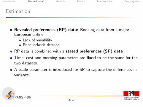
Estimation
Revealed preferences (RP) data: Booking data from a majorEuropean airline
Lack of variabilityPrice inelastic demand
RP data is combined with a stated preferences (SP) data
Time, cost and morning parameters are fixed to be the same for thetwo datasets.
A scale parameter is introduced for SP to capture the differences invariance.
4/ 21

Introduction Demand model Heuristic Results Transformation On-going work
Market shares
Market share for itinerary i in market segment s:
msi =exp(Vi (pi ,zi ,β))
∑j∈Is
exp(Vj (pj ,zj ,β))
Spill and recapture information in airline fleet assignment
Pricing decision
5/ 21

Introduction Demand model Heuristic Results Transformation On-going work
Integrated airline scheduling, fleeting and pricing
Decision variables:
xk,f : binary, assignment of aircraft k to flight f
πhk,f : allocated seats for class h on flight f aircraft k
pi : price of itinerary i
di : demand of itinerary i
ti ,j : spilled passengers from itinerary i to j
6/ 21

Introduction Demand model Heuristic Results Transformation On-going work
Integrated model - Scheduling & fleeting
Max ∑h∈H
∑s∈Sh
∑i∈(Is \I
′s )
(di − ∑j∈Is
ti ,j + ∑
j∈(Is \I′s )
tj ,i bj ,i )pi − ∑k∈Kf ∈F
Ck,f xk,f : revenue - cost (1)
s.t. ∑k∈K
xk,f = 1: mandatory flights ∀f ∈ F M (2)
∑k∈K
xk,f ≤ 1: optional flights ∀f ∈ F O (3)
yk,a,t− + ∑f ∈In(k,a,t)
xk,f = yk,a,t+ + ∑f ∈Out(k,a,t)
xk,f : flow conservation ∀[k,a,t] ∈N (4)
∑a∈A
yk,a,minE−a
+ ∑f ∈CT
xk,f ≤ Rk : fleet availability ∀k ∈ K (5)
yk,a,minE−a
= yk,a,maxE+
a: cyclic schedule ∀k ∈ K ,a ∈ A (6)
∑h∈H
πhk,f = Qk xk,f : seat capacity ∀f ∈ F ,k ∈ K (7)
xk,f ∈ {0,1} ∀k ∈ K , f ∈ F (8)
yk,a,t ≥ 0 ∀[k,a,t] ∈N (9)
Itinerary-based fleet assignment & Spill and recapture spill
Lohatepanont and Barnhart 2004
7/ 21
Introduction Demand model Heuristic Results Transformation On-going work
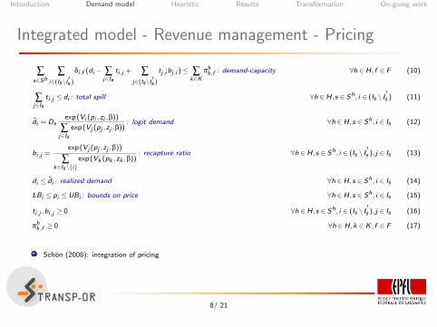
Integrated model - Revenue management - Pricing
∑s∈Sh
∑i∈(Is \I
′s )
δi ,f (di − ∑j∈Is
ti ,j + ∑j∈(Is \I
′s )
tj ,i bj ,i )≤ ∑k∈K
πhk,f : demand-capacity ∀h ∈H, f ∈ F (10)
∑j∈Is
ti ,j ≤ di : total spill ∀h ∈H,s ∈ Sh , i ∈ (Is \ I′s ) (11)
di = Dsexp(Vi (pi ,zi ,β))
∑j∈Is
exp(Vj (pj ,zj ,β)): logit demand ∀h ∈H,s ∈ Sh , i ∈ Is (12)
bi ,j =exp(Vj (pj ,zj ,β))
∑k∈Is \{i}
exp(Vk (pk ,zk ,β)): recapture ratio ∀h ∈H,s ∈ Sh , i ∈ (Is \ I
′s ), j ∈ Is (13)
di ≤ di : realized demand ∀h ∈H,s ∈ Sh , i ∈ Is (14)
LBi ≤ pi ≤ UBi : bounds on price ∀h ∈H,s ∈ Sh , i ∈ Is (15)
ti ,j ,bi ,j ≥ 0 ∀h ∈H,s ∈ Sh , i ∈ (Is \ I′s ), j ∈ Is (16)
πhk,f ≥ 0 ∀h ∈H,k ∈ K , f ∈ F (17)
Schon (2008): integration of pricing
8/ 21

Introduction Demand model Heuristic Results Transformation On-going work
Heuristic method
Mixed Integer Non-convex Problem
We devised a heuristic procedure based on two subproblems:
FAMLS : price-inelastic schedule planning model ⇒ MILP
Prices fixedOptimizes the schedule design and fleet assignment
REVLS : Revenue management with fixed capacity ⇒ NLP
Schedule design and fleet assignment fixedOptimizes the revenue
Local search based on spill information
9/ 21

Data
no airports flightsflights perroute
demand perflight
fleet composition
1 3 10 1.67 51.90 2 50-372 3 11 2.75 83.10 2 117-503 3 12 2.00 113.80 2 164-1004 3 12 2.00 113.80 6 164-146-128-124-107-1005 3 26 4.33 56.10 3 100-50-376 3 19 3.17 96.70 3 164-117-727 3 19 3.17 96.70 5 124-107-100-85-728 3 12 3.00 193.40 3 293-195-1649 3 33 8.25 71.90 3 117-70-37
10 3 32 5.33 100.50 3 164-117-8511 3 32 5.33 100.50 5 128-124-107-100-8512 2 11 5.50 173.70 3 293-164-12713 4 39 4.88 64.50 4 117-85-50-3714 4 23 3.83 86.10 4 117-85-70-5015 4 19 3.17 101.40 4 134-117-100-8516 4 19 3.17 101.40 5 128-124-107-100-8517 4 15 1.88 58.10 5 117-85-70-50-3718 4 14 2.33 87.60 5 134-117-85-70-5019 4 13 2.60 100.10 5 164-134-117-100-85
20 3 33 8.25 71.90 4 85-70-50-3521 3 46 7.67 86.85 5 128-124-107-100-8522 7 48 2.29 101.94 4 124-107-100-8523 3 61 15.25 69.15 4 117-85-50-3724 8 77 2.08 67.84 4 117-85-50-3725 8 97 3.46 90.84 5 164-117-100-85-50
Data instances are derived from ROADEF 2009 dataset.

Computational results
BONMIN Sequential Local search heuristicIntegrated model approach (SA) Average over 5 replications
ProfitTime
Profit% deviation Time
Profit%deviation %impr. Time
(sec) from BONMIN (sec) from BONMIN over SA (sec)1 15,091 2 15,091 0.00% 1 15,091 0.00% 0.00% 12 37,335 22 35,372 -5.26% 1 37,335 0.00% 5.55% 133 50,149 62 50,149 0.00% 1 50,149 0.00% 0.00% 14 46,037 2,807 43,990 -4.45% 1 46,037 0.00% 4.65% 35 70,904 1,580 69,901 -1.41% 1 70,679 -0.32% 1.11% 66 82,311 1,351 82,311 0.00% 1 82,311 0.00% 0.00% 17 87,212 32,400 84,186 -3.47% 1 87,212 0.00% 3.59% 608 779,819 8,137 779,819 0.00% 1 779,819 0.00% 0.00% 19 135,656 666 135,656 0.00% 2 135,656 0.00% 0.00% 2
10 107,927 482 107,927 0.00% 1 107,927 0.00% 0.00% 111 85,820 31,705 85,535 -0.33% 2 85,820 0.00% 0.33% 8812 858,544 5,598 854,902 -0.42% 1 858,544 0.00% 0.43% 113 112,881 32,713 109,906 -2.64% 1 112,881 0.00% 2.71% 15114 85,808 10,643 82,440 -3.93% 1 85,808 0.00% 4.09% 915 49,448 33 49,448 0.00% 1 49,448 0.00% 0.00% 116 38,205 240 37,100 -2.89% 1 38,205 0.00% 2.98% 117 27,076 35 27,076 0.00% 1 27,076 0.00% 0.00% 118 45,070 78 44,339 -1.62% 1 45,070 0.00% 1.65% 119 26,486 13 26,486 0.00% 1 26,486 0.00% 0.00% 1
20 146,773 30 846 146,464 -0.21% 1 147,506 0.50% 0.71% 40621 194,987 4,963 210,134 7.77% 10 214,251 9.88% 1.96% 1,49922 152,126 68,864 158,978 4.50% 2 159,258 4.69% 0.18% 3923 227,643 40,862 226,615 -0.45% 12 227,284 -0.16% 0.30% 1,28324 153,384 59,708 154,301 0.60% 4 158,099 3.07% 2.46% 2,31425 313,943 82,780 331,920 5.73% 13 332,744 5.99% 0.25% 1,451

Introduction Demand model Heuristic Results Transformation On-going work
Sensitivity Analysis
Leg-based FAM IFAM – choice-
based recapture
IFAM – choice-based recapture &
pricing
Fleeting & Scheduling Decisions
RMM – choice based recapture / pricing
Resulting Profit
12/ 21

Introduction Demand model Heuristic Results Transformation On-going work
Sensitivity to demand fluctuations
Total market segment demand is assumed to be known
Fluctuations in reality
Average demand is perturbed in a range [-30%, +30%]
For each average demand 500 simulations with Poisson
13/ 21

Sensitivity to demand fluctuations
25000
35000
45000
55000
65000
75000
85000
95000
105000
-30% -25% -20% -15% -10% -5% 0% 5% 10% 15% 20% 25% 30%
Prof
it
Perturbation on average demand
FAM
IFAM recapture
IFAM recapture & pricing
23 flights 4 aircraft types

Sensitivity to demand fluctuations
-50000
0
50000
100000
150000
200000
250000
-30% -25% -20% -15% -10% -5% 0% 5% 10% 15% 20% 25% 30%
Prof
it
Perturbation on average demand
FAM
IFAM recapture
IFAM recapture & pricing
77 flights 4 aircraft types - heuristic solution

Introduction Demand model Heuristic Results Transformation On-going work
Transformation of the logit model
msi =exp(Vi )
∑j∈Is
exp(Vj ), Vi = β ln(pi ) + ci
A new variable υs = 1
∑j∈Is
exp(Vj )
msi = υs exp(β ln(pi ) + ci )
∑i∈Is
msi = 1
υs ≥ 0
16/ 21

Introduction Demand model Heuristic Results Transformation On-going work
Transformation of the logit model
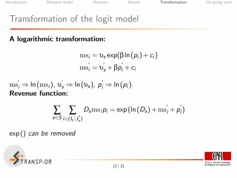
A logarithmic transformation:
msi = υs exp(β ln(pi ) + ci )
ms′i = υ
′s + βp
′i + ci
ms′i ⇒ ln(msi ), υ
′s ⇒ ln(υs), p
′i ⇒ ln(pi ).
17/ 21
Introduction Demand model Heuristic Results Transformation On-going work
Transformation of the logit model
A logarithmic transformation:
msi = υs exp(β ln(pi ) + ci )
ms′i = υ
′s + βp
′i + ci
ms′i ⇒ ln(msi ), υ
′s ⇒ ln(υs), p
′i ⇒ ln(pi ).
Revenue function:
∑s∈S
∑i∈(Is\I ′s )
Dsmsipi = exp(ln(Ds) +ms′i +p
′i )
exp() can be removed
17/ 21

Introduction Demand model Heuristic Results Transformation On-going work
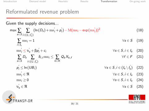
Reformulated revenue problem
Given the supply decisions...
max ∑s∈S
∑i∈(Is\I ′s )
(ln(Ds ) +ms′
i +p′
i )−M(msi − exp(ms′
i ))2 (18)
∑i∈Is
msi = 1 ∀s ∈ S (19)
ms′
i = υ′s + βp
′
i + ci ∀s ∈ S , i ∈ Is (20)
∑s∈S
Ds ∑i∈(Is\I ′s )
δi ,f msi ≤ ∑k∈K
QkXk,f ∀f ∈ F (21)
p′
i ≤ ln(UBi ) ∀s ∈ S , i ∈ (Is \ I′s ) (22)
ms′
i ∈ℜ ∀s ∈ S , i ∈ Is (23)
msi ≥ 0 ∀s ∈ S , i ∈ Is (24)
υ′s ∈ℜ ∀s ∈ S (25)
18/ 21
Introduction Demand model Heuristic Results Transformation On-going work
Reformulated revenue problem
Given the supply decisions...
max ∑s∈S
∑i∈(Is\I ′s )
(ln(Ds ) +ms′
i +p′
i )−M(msi − exp(ms′
i ))2 (18)
∑i∈Is
msi = 1 ∀s ∈ S (19)
ms′
i ≤ υ′s + βp
′
i + ci ∀s ∈ S , i ∈ Is (20)
∑s∈S
Ds ∑i∈(Is\I ′s )
δi ,f msi ≤ ∑k∈K
QkXk,f ∀f ∈ F (21)
p′
i ≤ ln(UBi ) ∀s ∈ S , i ∈ (Is \ I′s ) (22)
ms′
i ∈ℜ ∀s ∈ S , i ∈ Is (23)
msi ≥ 0 ∀s ∈ S , i ∈ Is (24)
υ′s ∈ℜ ∀s ∈ S (25)
18/ 21

Introduction Demand model Heuristic Results Transformation On-going work
Added value of the reformulation
Even for a small instance with 11 flights, 2 aircraft types
If the elasticity is very high, non-convexity misleads
Original - BONMIN Reformulated - MOSEKProfit: -12,516.2 Profit: 6,816.7Op. costs: 140,207 Op. costs: 140,207
ms price ms price1 0.80 140 0.80 1402 0.80 140 0.80 1403 0.13 250 0.13 2314 0.29 200 0.29 2005 0.30 200 0.27 2006 0 - 0.12 1207 0 - 0.13 1808 0.29 237 0.29 1989 0 - 0.13 200
10 0 - 0.12 22511 0.30 228 0.22 208
19/ 21

Introduction Demand model Heuristic Results Transformation On-going work
Conclusions
The integrated model has promising results
... which motivates the effort in devising solution methodologies
Logarithmic transformation provides a concave formulation of therevenue problem
... is expected to facilitate efficient solution methodologies
20/ 21

Introduction Demand model Heuristic Results Transformation On-going work
On-going work
Tests with the reformulated problem
The framework is flexible for the integration of advanced demandmodels
∑i∈Is
(ln(Ds) +ms′i +p
′i )⇒ ∑
i∈Is
∑n∈N
p′i +Prob
′i ,n
Generalized framework for the integration of endogenous demandmodels
21/ 21

Introduction Demand model Heuristic Results Transformation On-going work
On-going work
Tests with the reformulated problem
The framework is flexible for the integration of advanced demandmodels
∑i∈Is
(ln(Ds) +ms′i +p
′i )⇒ ∑
i∈Is
∑n∈N
p′i +Prob
′i ,n
Generalized framework for the integration of endogenous demandmodels
Writing the thesis!!!
Thank you for your attention!
21/ 21

Introduction Demand model Heuristic Results Transformation On-going work
Logit behavior
22/ 21

Introduction Demand model Heuristic Results Transformation On-going work
Itinerary choice model
Market share and demand for itinerary i in market segment s:
msi =exp(Vi (pi ,zi ,β))
∑j∈Is
exp(Vj (pj ,zj ,β))⇒ di = Dsmsi
- Ds is the total expected demand for market segment s.
Spill and recapture effects: Capacity shortage ⇒ passengers maybe recaptured by other itineraries (instead of their desired itineraries)
Recapture ratio is given by:
bi ,j =exp(Vj (pj ,zj ,β))
∑k∈Is\{i}
exp(Vk (pk ,zk ,β))
23/ 21

Introduction Demand model Heuristic Results Transformation On-going work
Itinerary choice model
Value of time (VOT):
VOTi =∂Vi/∂timei
∂Vi/∂costi
=βtime · costi
βcost
For the same OD pair...
VOT for economy, non-stop: 8 e/hourVOT for economy, one-stop: 19.8, 11, 9.2 e/hourVOT for business, non-stop: 21.7 e/hour
24/ 21

Introduction Demand model Heuristic Results Transformation On-going work
Spill and recapture model
Forecasted demand for an itinerary is 120
Airline considers assigning a capacity of 100 to the associated flight
Estimated spilled passengers is 20
If these people are redirected to other itineraries in the market whatpercantage will accept?
25/ 21

Introduction Demand model Heuristic Results Transformation On-going work
Improvement due to the local search
Sequential Random Neighborhood% Improvement
approach (SA) neighborhood based on spill
Profit Profit Time(sec) Profit Time(sec)Quality of Reduction
the solution in time2 35,372 37,335 116 37,335 13 - 89.10%4 43,990 44,302 27 46,037 3 3.92% 88.88%5 69,901 No imp. over SA 70,679 6 1.11% -7 84,186 85,335 1,649 87,212 60 2.20% 96.36%8 904,054 906,791 209 906,791 2 - 99.04%
11 93,920 No imp. over SA 94,203 10 0.30% -12 854,902 No imp. over SA 858,545 1 0.43% -13 137,428 No imp. over SA 138,575 173 0.83% -14 93,347 96,365 943 96,486 89 0.13% 90.56%16 37,100 38,205 6 38,205 1 - 80.65%18 52,369 53,128 334 53,128 1 - 99.80%
20 146,464 No imp. over SA 147,506 380 0.71% -21 217,169 No imp. over SA 219,136 1,395 0.91% -22 163,114 No imp. over SA 163,393 126 0.17% -23 226,615 No imp. over SA 227,284 1,283 0.30% -24 208,561 No imp. over SA 210,395 791 0.88% -25 469,136 No imp. over SA 470,494 1,117 0.29% -
26/ 21

Introduction Demand model Heuristic Results Transformation On-going work
A small example
2 airports CDG-MRS
4 flights - all are mandatory
2 aircraft types: 37-50 seats
We start with an initial FAM solution:
AC1 AC2F1 XF2 XF3 XF4 X
27/ 21

Introduction Demand model Heuristic Results Transformation On-going work
A small example - GBD iterations
Iteration 1 Iteration 2Sub Master Sub Master
12522.8 16923.4 10734.4 14822.8LB UB LB UB
12522.8 16923.4 =⇒ 12522.8 14822.8AC1 AC2 AC1 AC2
F1 X F1 XF2 X F2 XF3 X F3 XF4 X F4 X
Iteration 3 Iteration 4Sub Master Sub Master
12696.8 14822.8 12474.4 12696.8LB UB LB UB
12696.8 14822.8 =⇒ 12696.8 12696.8AC1 AC2 AC1 AC2
F1 X F1 XF2 X F2 XF3 X F3 XF4 X F4 X
28/ 21