-e

ANALYSIS OF A MULTI-ITEM INVENTORY PROBLEM

USING OPTIMAL POLICY SURFACES

by

Helmut Schneider

University of North Carolinaat Chapel Hill, NC 27514

-e

1. Introduction

In this paper we shall consider a multi-item inventory problem with

unspecified single-item unit costs. Rather than examining a single cost

function, we shall deal with an approach which incorporates aggregate

objectives and constraints. The objectives are low investment, low total

costs and high service-level. The constraints are storage room capacity

and available workload for handling the orders. These capacities might be

increased or decreased in certain fixed quantities; such changes in workload

and storage room incur costs which are independent of whether or not these

capacities are used to their full extent. The objectives are conflicting

and in many real world problems there seems to be no single cost function

for determining an optimal decision. This is due to the fact that there is

no decision unity; instead, there are different departments, different

managers and differing interests involved. How much the company should

invest in inventory and what service level should be required cannot be

determined simply by. evaluating a single cost function, but is rather a

result of intensive discussions. What operations research can offer is a

description of the relationship between investment and service-level; i.e.,

for a certain investment we are able to maximize the service-level under

the constraints of storage room and workload. Furthermore we might study

the effect upon an alteration of the constraints. This enables the

management to find an "appropriate" decision weighing the different interests

ascertaining that there is no solution with lower total costs and higher

service-level.

Despite the enormous number of papers on inventory models there are

only a few articles concerning this important problem. Most papers start

-

-2-

by assuming that marginal holding, shortage and ordering costs are given.

But marginal ordering costs are difficult to measure. Most suggested

approaches for determining ordering costs in the accounting literature

result in average rather than marginal costs [15]. In practice there is

usually a certain workload available which might be increased in fixed

quantities. Assigning average order costs therefore does not solve this

particular inventory problem. Holding costs should be composed not only

of the cost for capital but also of marginal costs taking into considera­

tion a storage room restriction. The use of shortage costs in inventory

theory has not been adopted by most practitioners [2] since there is no

basis for their measurement in accounting methodology [15].

Only a few authors deal with an aggregate inventory problem as described

above.

Starr and Miller [13] have considered an "optimal policy curve!' for

deterministic demand. Schrady and Choe [11] considered a continuous review

inventory system with constraints. Gardner and Dannenbring [3] extended

Starr's and Miller's approach by considering a continuous review stochastic

model. They presented a method that avoids cost measurement problems and

incorporates aggregate objectives and constraints. They describe a

procedure for obtaining an optimal policy surface, the axes of which are

measured in aggregate terms: the percentage of inventory shortages, as a

measure of customer service; the workload in terms of the number of annual

stock replenishment orders; and total investment, the sum of cycle and

safety stocks. Aggregate inventory decisions are defined as the selection

of a combination of the three variables. This model obviously reflects

the true decision problem in practice much better than a single-item cost

model. In fact data simulation is frequently employed in practice to

solve decision problems described above.

-

·e

-3-

Unfortunately the underlying inventory model, considered by Gardner

and Dannenbring, has some disadvantages which makes it inapplicable in many

situations. Most of the inventory systems installed in practice have

periodic review and not continuous review [5]. It has been shown that,

given a certain inventory policy, the service-level turns out to be very

different in a periodic and in a continuous review system [9]. Further­

more we should be aware that there are different definitions of service­

levels [10], which result in very different ordering policies.

In the present paper a similar approach to that of Gardner and

Dannenbring is used. But there are some essential differences. First, a

periodic review multi-item inventory model -rs considered. Second, we

consider only two objectives, investment and service-level, subject to

workload and storage room .restrictions. It seems to be more realistic to

begin with a given workload and storage room, which can be expanded in fixed

quantities, rather than to assume that workload and storage room are

continuous variables. Furthermore an overall cost evaluation is considered

including costs of investment, storage room and workload.

An interactive algorithm is presented which allows the selection of a

combination of service-level, investment, workload and storage room which

is "appropriate"for the management. This method produces combinations

which lie on an optimal surface.

Since in our method there are some approximations involved, we shall

prove the validity of the approximation formulas by means of a Monte Carlo

study in the final section.

-

2. The Model

Consider an inventory model withn items. The stock of every item is

inspected at the beginning of a review period and an order is placed for

those items for which the stock level has fallen to the reorder point.

After a known lead time A the orders will arrive. The demand of an item in

different periods is a random variable with known distribution. Let us

define for item k. k-l.2.3 ••••• n.

~t - inventory on hand plus on order at the beginning of period t. before

an order is placed.

Qkt - order which is placed at the beginning~of period t

rkt - stochastic demand in period t. The demand in successive periods is a

sequence of independent and identically distribuged random variables

2with cdf Fk (r). mean l1t and variance crk •

Pk -price of item k.

Furthermore. it is assumed that demand which cannot be immediately

satisfied is backordered. We discuss a stationary inventory model and thus

it is sufficient to consider a single period inventory model ~here the

distribution of ~t is the stationary distribution 1jJ(x) [6). We will also

assume that a service level y • which is defined as

e-

y = 1-cumulative backorders per period

average demand per period

is an appropriate measure of customer service for product k-l ••••• n.

Notice that this definition of a service level is equivalent to assigning

shortage costs which are dependent on the amount of items short and the

length of time the shortage lasts. A formal proof is given in [9). This

-

·e

-5-

type of shortage cost is considered by most authors [4]. [11]. [14].

In what follows we consider two objectives:

01: minimize the total investment as the sum of cycle and safety stock

02: maximize the service level y and two constraints

and two constraints

Cl

: the number of stock replenishment orders is restricted by the workload

capacity

C2: there is a storage room capacity restriction

This two-objective-decision problem is solved by determining the optimal.-.:..

policy surface. For every point on the surface it holds that none of the

objectives can be improved without diminishing the other. Before proceeding

we shall make some remarks concerning the objectives and constraints. The

objectives reflect of course cost considerations and the constraints are

associated with costs which become relevant if alterations of the constraints

are allowed. With 01 we only control the variable holding costs induced by

invested capital. If the storage room is fixed the costs for holding this

room are fixed too and thus irrelevant for a decision. But often it is the

case that storage room is rented in certain quantities and hence the costs

for holding a storage capacity becomes relevant for a decision. The same

is true for the workload restriction. We therefore cons.ider a second set

of objectives without constraints.

04: minimize total costs involving cost for workload. cost for invested

capital, and cost for holding a storage room.

°5: maximize service level y

Both sets of objectives should be available for a decision process for

selecting an "appropriate" solution.

-

-6-

We shall now formally define our objectives and constraints. It is well

known that when given a single item inventory model of the type described

above an (s,S) policy is optimal [6]. We will thus consider (sk,Sk)

policies in our approach. Let

E[Iklsk,Sk] - expected inventory at the end of a period for product k

E[Qk!sk,Sk] - expected order quantity for product k

E[NOklsk,Sk] - expected number of orders per period for product k

E[CI\{sk,Sk}] - expected invested capital in inventory

E[NO\{Sk,Sk}] - expected number of orders per period

E[SRI{~,Sk}] - expected storage room

Note that

n

E[SR\{sk,Sk}l - L ~E[Iklsk,Skl

k-1

where ~.is the unit storage room for product k. We finally formulate

the two-objective-decision problem as

e-

subject to

-

(1)

-7-

E[SRI{Sk,Sk}] ~ Storage room capacity (SRR)

(WLR)

(3)

(4)

Considering a single item the expected values can be derived by [9].

+ Dk +L (~)+ I L (Sk-x)m(x)dx

o(5)

1l+M(Pk)

DL-(Sk)+ Jk L-(Sk-x)m(x)dx

o

(6)

(7)

·e

where (see [9]) M(-) and m(-)z

n(z) • F(z)+ J M(z-t)dFk(t).0.

+ -and Land L are defined by

are solutions of the renewal equationsz

m(z) • f(z)+ J ~(z-t)fk(t)dto

x~O

x~O

A+lwhere f k (t) is the pdf of demand in lead time plus review time. Note

that Dk • Sk-sk. Although an exact solution, i.e. the determination of the

optimal policy surface, is in principle possible, we will not recommend

it since the approximation, provided below, will give such excellent

results that there is no incentive to carry out the extraordinary high

computations. Our approximation is based on empirical results [14] that

there is only little loss of optimality if the optimization is separated

-8-

in determining first Dk • Sk-sk and afterwards sk. Furthermore, we consider

the expected values under the realistic assumption that Dk is large and we

are thus able to simplify the expressions (5) to (7), an approach which was

introduced by Robert.s [8 ] ~ Following these principles we derive the

simplified expected values

(8)

(9)

y(s ,5 ) • 1­k k(10)

The expression (8) is derived in the appendix; (9) is a well-known limiting

theorem of the renewal function M(D) [12] and (10) was derived in [9].

Since the constraint (4) will always be active we can solve this

optimization problem using the Lagrange method. Let

n n1.(Ql,···,Qn'p)· L PkE[IkIQk] + p[ LE[NOk!Qk] - WLR] (11)

k-l k-l

A straightforward application of the Lagrange methQd yields

e·

k-l, ••• ,n

-

(12)

-9-

and

(13)

The reorder points sk can now be calculated in a second step for various

service levels y. We determine sk by equation (10).

The cycle plus safety stock for product kand fixed service-level is

then

(14)

and thus the total investment is

and the expected total storage room is

which are both functions of the service level y. The· latter value is now

compared with the storage room capacity. The service level can be increased

as long as the storage room constraint is not active. We obtain a diagram

which shows the investment versus service-level y; this diagram will end at

y' which marks the maximum service-level at which the storage room constraint

becomes active. In addition a diagram which gives the total costs (for

investment plus fixed costs for the storage room capacity plus fixed costs

for the.workload capacity) versus service-level can be presented (see

figures 2 and 3). In contrast to the unit single item costs these fixed costs

are easy to determine. These diagrams are the basics for selecting an

"appropriate" service-level and investment by the management. The steps for

obtaining the diagrams are summarized in the following algorithm.

-

-10-

Figure 1: Algorithm

minimize capital invested ininventory subject to workloadrestriction (determination ofDk , and cycle stock)

maximize service level subjectto storage room restr1~tion

(determination of reorder pointssk and safety stock)

output: diagram a) service-levelvs investment(b) service-level vstotal costs

Yes~------Iselection of new storage room capacit~

l no

Yes

no

-

-11-

Example

In this subsection we shall consider an example with only 100 items

to describe the algorithm. In practice the service-level of items varies

from product to product. Some products, for example, are more vital than

others. Usually, however, one is able to classify the items and put them

into certain groups which have the same service-level requirements.

We thus define m groups such that

let nj be the number of products in subgroup j then

1 n 1 m -~

Y·- LY -- Lngoyn k-l k n j-l j j

which yields to the restriction.

1 mn L n j

gj - 1

j-l

Furthermore

(15)

(16)

The problem of assigning Yk is thus reduced to determining m numbers gj

which fulfill (15) and (16). This will usually be possible in a reasonable

way.

We shall now consider a situation in which the management has to

decide how much to invest during the year to come and what service-level

should be required. There is a certain workload available which allows

22 orders per week. The .. cost of this workload is $115.000 per year. Free

handling capacity cannot be used for other purposes. An increase or

decrease of workload is only possible in quantities which are equivalent

to 4 orders per week. The cost for such a workload quantum is $15.000

per year. There is also storage room available which allows for the

storage of 60.000 units. The cost for renting the storage room is

-

-12-

$130,000 per year. Increase or decrease is only possible in quantities of

10,000 units whictt will cause costs of $20,000 per year. The following data

are assumed to be known

mean demand: ~. 20+9. 89 (k-l) k • 1,2, ••• ,100

variance: 2 2 2k • 1,2, ••• ,100ok • c~

c • 0.2, 0.4, 0.6, 0.8, 1.2, 1.6

unit storage roomof product k: is randomly chosen to be in the interval [0.5,1.5]

lead time: is randomly chosen to be {2,3,4,5,6,7,8}-:...

price:

service level:

Pk • 500/~ k· 1,2, •.• ,100

5 groups of 20 products with the service levels O.Sy,

0.9y, y, l.ly, 1.2y

We assume a 10% interest for the invested capital. The algorithm is demon-

strated for c • 0.2. The management assigns an interval for the service-

level 60% ~ Y ~ 100%. According to the algorithm the following diagram is

plotted. Due to the workload restriction for handling and the storage room

restriction the maximum average service level is 79.5%, thus the diagram

ends at that point.

-

-13-

Figure 2: Service-level versus investment

Service level

The total costs are presented in the next diagram. The total costs are

the sum of the costs for storage room, workload and invested capital.

-14-

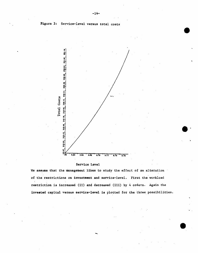
Figure 3: Service-level versus total costs

·=~

:"··•~"·••=:•=~

•-~ "~

"~

0 :u "~ ·~ ~

~ :0 "H

~:"•· e~ ."·:"

Service Level

We assume that the management likes to study the effect of an alteration

of the restrictions on investment and service-level. First the workload

restriction is increased (II) and decreased (III) by 4 orders. Again the

invested capital versus service-level is plotted for the three possibilities.

-15-

Figure 4: The effect of an alteration of the workloadrestriction. I) initial situation, II) increase,III) decrease of workload restriction.

-e

Servico level

We see that a reduction of workload (curve III) results in a lower available

service-level while an increase allows a higher service-level than 79.5%.

This is caused by a change of the cycle stock, which decreases (curve III)

or increases (curve II) the available storage room for safety stock.

Diagram 5 gives the total costs for the alternatives.

-

-16-

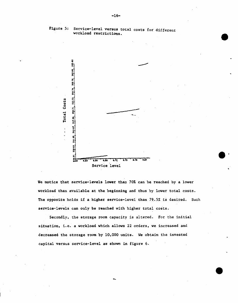
Figure 5: Service-level versus total costs for differentworkload restrictions •

..~..•...~..:~

::;:.-:::

al.....

.u ..;al :::0tJ '-...~ ::III.u ..0 '"!... ...·.....

'"!··....'"!

·....•......·..... •..

---

------..... :..

e·Service level

We notice that service-levels lower than 70% can be reached by a lower

workload than available at the beginning and thus by lower total costs.

The opposite holds if a higher service-level than 79,. 5%i9 desired. Such

service-levels can only be reached with higher total costs.

Secondly. the storage room capacity is altered. For the initial

situation, i.e. a workload which allows 22 orders, we increased and

decreased the storage room by 10,000 units. We obtain the invested

capital versus service-level as shown in figure 6.

-

-17-

Figure 6: Service-level versus investment for different storageroom restrictions

..-::

.-.-..

::,.;...-....

•• I

Service Level

.­..

.-:

Since the workload restriction is fixed. the cycle stock is constant and

only the safety stock increases. which results in a curve ending at a

service-level of 82.5%.

Figure 7 gives the total costs of the three alternatives.

-

-18-

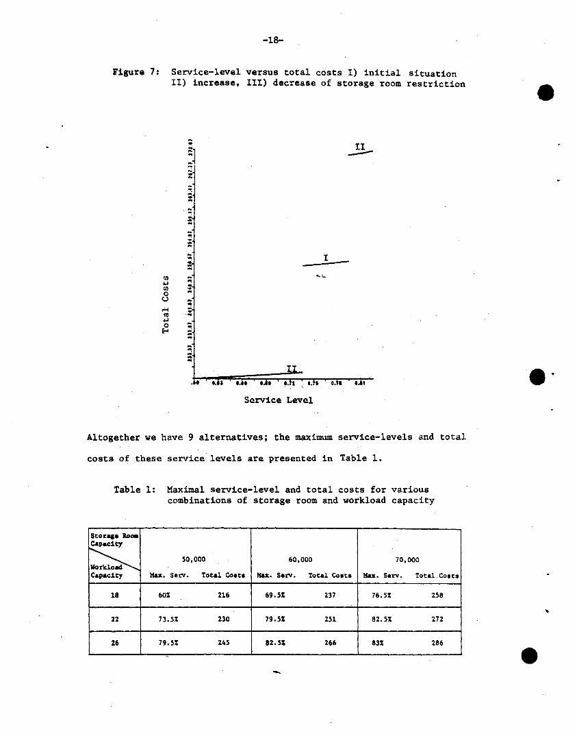
Figure 7: Service-level versus total costs I) initial situationII) increase. III) decrease of storage room restriction

~

~:l~

~....-....=~..::-~..::~....::

CIl ~

4-l..

CIl :0 ..

to}~

"!r'-! :til4-l

~0 ..E-I ,.;....

~........•

II---

I

Service Level

Altogether we have 9 alternatives; the maximum service-levels and total

costs of these service levels are presented in Table 1.

Table 1: Maximal service-level and total costs for variouscombinations of storage room and workload capacity

Storq. IlooaCapadty

~ 50,000 60,000 70,000

Capacity Max. Servo Total COlta Max. Servo Total COlts Max. Servo Total Costs

18 60% 216 69.5% 237 76.5% 258

22 73.5% 230 79.5% 251 82.5% 272

26 79.5% 245 82.5% 266 83% 286,

-

-19-

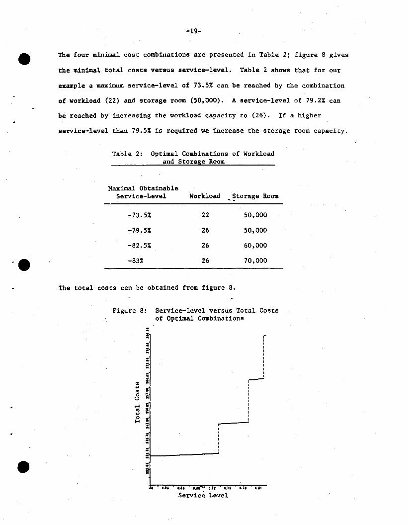
The four minimal cost combinations are presented in Table 2; figure 8 gives

the minimal total costs versus service-level. Table 2 shows that for our

example a maximum service-level of 73.5% can be reached by the combination

of workload (22) and storage room (50,000). A service-level of 79.2% can

be reached by increasing the workload capacity to (26). If a higher

service-level than 79.5% is required we increase the storage room capacity.

Table 2: Optimal Combinations of Workloadand Storage Room

Maximal ObtainableService-Level Workload _~torage Room

-73.5% 22 50,000

-79.5% 26 50,000

-82.5% 26 60.000

-83% 26 70.000

The total costs can be obtained from figure 8.

Figure 8: Service-level versus Total Costsof Optimal Combinations

:..= i

I

~IIII· I

5 III.. I

: I

al = r---I..,

:; Ial I0 .. I

U .. II

~.. I~

I111 ::.., I

0 I· IE-i S .FI.. I

""I

= II

~II

··o. 2

Service Level

-20-

The management now has all the necessary information to decide what

service-level and corresponding investment should be selected. and whether

or not the workload and the storage room restrictions should be altered.

We notice that with the selection of a certain point on one of the

curves presented above we determined the optimal inventory policy as well~

i.e. the set {sk,Sk}.

3. Validation of the Model by Monte Carlo Simulation

The purpose of the simulation prOVided in this section is twofold.

First. we want to use the simulation results to test the accuracy of the

approximation formulas derived in section 2_~ Second. we investigate the

variance of the various measures of system performance such as handling

used. inventory on hand. invested capital over the periods. Since the

restrictions are met by expected values. we have to be careful that the

variance is not too large.

We have performed 6 simulations for different demand structures, 1.e.

c - 0.2. 0.4. 0.6. 0.8. 1.2. 1.6. For c~ O.S a normal distribution was

used; otherwise the gamma distribution was found to be appropriate [9].

Notice that for increasing c the demand becomes very erratic. The

simulations were run for workload WL - 22 and service level y - '0.82. The

theoretic results for inventory on hand and invested capital are given

in Table 3.

-

..

-21-

Table 3: Theoretical results (y • 0.82 required) for mean storage roomand invested capital.

Expected Expected Invested Capitalc • cr/'fJ. Storage Room In Inventory

Used In $

0.2 67.312 68.855

0.4 86.185 87.167

0.6 120.282 120.445

0.8 162.687 163.212

1.2 279.741 283.268-:..

1.6 440.667 451.172

Table 4 gives the simulation results with 1000 periods and 50 repetitions.'_ Table 4: Simulation results for mean storage room.mean invested capital. mean handling andmean service-level.

Storage Iooa U.ed

c • a/lJ HandlingMean Std t.% Mean Std t.%

0.2 68.322 60 +1.5 22 0.01 +0.1

0.4 86.761 47 +0.6 22 0.01 +0.1

0.6 122.373 61 +1.7 21.8 0.01 -0.7

0.8 166.104 187 +2.1 21.9 0.02 -0.6

1.2 286.735 226 +2.5 21.6 0.01 -1.9

1.6 445.082 261 +1.0 22 0.01 -0".2

Inve.ted CapitalService-Level

Kean Std Kean Kean - y

0.2 69.938 51 +1.6 82% 0

0.4 87.830 43 +0.8 82% 0

0.6 122.855 53 +2.0 82.5% 0.5

0.8 167.129 115 +2.4 84% 2

1.2 289.783 183 +2.3 83.5% 1.5

tit 1.6 452.373 222 +0.2 86% 4

t.% is percentage of deviation fro- theoretic value-

-22-

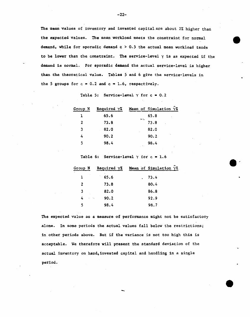
The mean values of inventory and invested capital are about 2% higher than

the expected values. The mean workload meets the constraint for normal

demand, while for sporadic demand c > 0.5 the actual mean workload tends

to be lower than the constraint. The service-level y is as expected if the

demand is normal. For sporadic demand the actual service-level is higher

than the theoretical value. Tables 5 and 6 give the service-levels in

the 5 groups for c • 0.2 and c • 1.6, respectively.

Table 5: Service-level y for c • 0.2

Required xX Mean of '"Group N Simulation y%

1 65.6 65.8~.-

2 73.8 73.8

3 82.0 82.0

4 90.2 90.2

5 98.4 98.4

Table 6: Service-level y for c • 1.6

,..Group N Required x% Mean of Simulation y%

1 65.6 73.4

2 73.8 80.4

3 82.0 86.8

4 90.2 92.9

5 98.4 98.7

The expected value as a measure of performance might not be satisfactory

alone. In some periods the actual values fall below the restrictions;

in other periods above. But if the variance is not too high this is

acceptable. We therefore will present the standard deviation of the

actual inventory on hand, invested capital and handling in a single

period.

-

..

-23-

We would expect that as demand becomes more erratic the fluctuation

of the mentioned variables increases and thus results in a higher

standard deviation. But as we see from Table 7, while the standard

deviation of demand increases from 0.2~ to 1.6~, the standard deviation

of the inventory on hand in a single period increases only from 0.1 x

inventory on hand to 0.75 x inventory on hand.

Table 7: The effect of demand structure on the performance of storageroom artd invested capital.

Storage Room Usedin 1000 Units Invested Capital Workload

-:..

c • (]/~ Mean Std Std/Mean Mean Std Std/Mean Mean Std Std/Mean

0.2 68 7 0.1 70 6 0.08 22 4.0 0.18

0.4 87 8 0.09 88 7 0.08 22 4.0 0.18

0.6 122 11 0.09 123 10 0.08 22 4.1 0.19-- 0.8 166 17 0.1 167 15 0.09 22 4.1 0.19

1.2 287 43 0.15 290 39 0.13 22 4.3 0.2• 1.6 445 64 0.15 452 57 0.13 22 4.4 0.2

To obtain a more precise picture of the actual performance of the inventory

system under consideration we studied the frequencies of inventory and

handling. Table 8 gives the frequency of inventory on hand in a single

period measured in terms of deviation from the theoretical expected value.

-

c.

-24-

Table 8: Frequency of inventory on hand

crIll 80% 90% 100% 110% 120% 130% 140% 150%

0.2 0.04 0.21 0.39 0.28 0.07 0.01 a a0.4 0.04 0.23 0.42 0.26 0.05 a a a0.6 0.02 0.18 0.47 0.29 0.04 0 0 a0.8 0.07 0~14 0.51 0.31 0.03 0.0 0 a1.2 0.003 0.14 0.62 0.27 0.006 0.002 0.002 0.011.6 0.001 0.18 0.71 0.09 0.004 0.002 0.002 0.01

-

•

-25-

Table 9: Frequencies of orders per period

c-a/lJ. 60% 70% 80% 90% 100% 110% 120% 130% 140% 150%

0.2 0.02 0.06 0.12 0.17 0.28 0.16 0.11 0.05 0.02 0.01

0.4 0.02 0.06 0.12 0.16 0.28 0.15 0.11 0.06 0.03 0.01

0.6 0.03 0.06 0.12 0.17 0.28 0.15 0.10 0.05 0.03 0.01

0.8 0.03 0.06 0.12 0.17 0.28 0.15 0.10 0.05 0.03 0.01

1.2 0.03 0.06 0.12 0.17 0.28 0.15 0.10 0.05 0.03 0.01

1.6 0.03 0.06 0.11 0.16 0.28 0.16 0.11 0.06 0.02 0.01

Cumula-tive 0.03 0.09 0.20 0.36 0.64 6~80 0.91 0.97 0.99 1.00

The reason for the unexpected result. namely that fluctuation decreases as

demand variation increases. is due to the correlation of the investigated

variables. The following figures show the autocorrelation function of

inventory and the number of orders for c - 0.2 and c - 1.6 respectively.

We see that for normal demand we obtain cycles of high inventory and a

high number of orders. This is due to the relatively high deterministic

part of normal demand. It is obvious that during every 4th and 5th period

a high number of orders arrives. If demand is sporadic there is no

significant correlation between the number of orders in different periods.

The inventory is highly autocorrelated as one would expect for sporadic

demand since there is no demand in most periods. But we also notice that

no cycles appear if demand is sporadic.

We might conclude from our simulation study that the performance of the

inventory system was close to that predicted by the theoretical model.

The modal values are the same as the expected values of the model. But

since the distribution of the variables under consideration tend to be

-

-26-

skewed to the right the average of actual inventory and invested capital

is 2% higher than the expected value. The service-levels are as

required. The variation of the variables are higher when demand has a

high deterministic part. i.e. c < 0.5. In this case we notice the

appearance of cycles in total inventory and orders. It seems that there

has been very little attention given to this problem up till now in

inventory literature.

-

•

•

---------------------------------------------~-----------------:I SS ~ ~ ; ; ; • £ ; • : • ; : ~ C ~ ~ : II ~~~~":~":~ .~~~~~~~~~-:~l• • • • • • • • • T • • • • f T T • • .:---------------------------------------------------------------:,I - . . . . . - . . ~ ; ~ : ~ : ! : ~ ~ c I: ~ i

-----------------------------------------------------------~---.

1-- S I I S - • a r • - c - • I - - I I II • = ~ .. . ~ 2 ; • .. ~ = _ : = _ ~ ! .. ....................... . . . . . . . . . . . . . . . . . . .

---------------------------------------------------------------'I - ,. .... ""-. .. . .. . . : : ~ : ~ :; :: : :: !; I,

: -------------------------------------------------------------

l.···-··--..---..··-.···-·...··-·--···-·----.·-~---··.....-.....I··r!'-r.--r;-'-·---~III ~ ~ ~ . ~ :; ~ ~ ~ ~ ": ~ ~ ~ ; , ~ , , -:.1.•:_.!..!..:..:..!..!..:..:..:..!_.!__:_.:__!__!__:..:__:__!..! - .. '" : : 2 : : e :! : S l C. ,

-----.------._-----------~--.__._----_.---~-------------- ---_.-Fig. 9a Correlation coefficient RO of

average inventory on hand.c .. 0.2

!~

] "

· :1..__..__...1 1 ••••••:••1..1.__.••.•1..1_ :

:1 I . II I I I I:I I

:1:1;1.................------....•...--...•.------....------_·······-1I Ii: ., i r: s ! .= ! ! 5 ! ,: 1 : : : ! i !II iii .; , i i ~ .; i iT .; .; T i .; .; i i---------------------------------------------------------------'I s :. : : : !: s ~ :. t •

._----------------.--.__._~-------------------_ ..-

Fig. 9b Correlation coefficient RO, ofaverage inventory on hand.c • 1.6

Fig. 9c Correlation coefficient RO ofhandling. c· 0.2

Fig. 9d Correlation coefficient RO ofhandling. c = 1.6

-

References

1. Alscher. T. and H. Schneider. Resolving a multi-item inventory problem·with unknown costs. Engineering Costs and Production Economics, ~,

9-15 (1982).

2. Brown, R.G. Decision Rules for Inventory Management. Holt, New York,1967.

3. Gardner. E.S. and D.G. Dannenbring. Using optimal policy surfaces toanalyze aggregate inventory tradeoffs. Management Science, Vol. 25.No.8.(August 1979).

4. Hadley.G. and T.M. Whitin. Analysis of Inventory Systems. Prentice-Hall.Englewood Cliffs. 1963.

5. IBM System 1360 inventory control (360 A-MF~X). Program descriptionmanual GH20-555-l. New York.

6. Karlin. S. Steady state solutions. In: Studies in the MathematicalTheory of Inventory and Production (K.T. Arrow, S. Karlin andH. Scarf, Eds.) Chapter 14. Stanford University Press. Stanford.

7. Peterson, R. and Silver. E.A. Decision Systems for Inventory Managementand Production Planning, New York: John Wiley, 1979.

8. Roberts, D.M. Approximations to optimal policies in dynamic inventorymodel. In: Studies in Applied Probability and Management Science(K.T. Arrow, S. Karlin and H. Scarf, Eds.) Stanford University Press.Stanford, 1962.

9. Schneider, H. Methods for determining the re-order point of an (s,S)ordering policy when a service-level is specified. J. Opere Res.Soc. Vol. 29, 12, 1181-1193, (1978).

10. Schneider, H. "Effect of service-levels on order-points or order-levelsin inventory models," Int. J. Prod. Res., Vol. 19, No.6, 615-631(1981).

11. Schrady, D.A. and Choe, V.E. '~ode1s for Multi-Item Continuous ReviewInventory Policies Subject to Constraints". Naval Res. Logist.Quart. Vol. 8, No.4 (December 1977).

12. Smith, W.L. Asymptotic renewal theorems. Proc. R. Soc., Edinb-64,9-48, (1954).

13. Starr. M.K. and Miller, D.W. Inventory control: Theory and practice.Prentice-Hall, Englewood Cliffs, N.J. (1962).

-

•

•

15.

Wagner. H.M. and Hagan. M.O. and Lundh. B. An empirical study of exactlyand approximately optimal inventory policies. Management Science.Vol 11, 690-723 (1965).

Ziegler, R.E. Criteria for measurement of the cost parameters of aneconomic order quantity inventory model. Unpublished Ph.D. Disserta­tion, University of North Carolina, 1973.

-

APPENDIX

We will show that the expected inventory on hand has the asymptotic

value

B[Ils,S] ~ D(l - ~Q) + s-~A+l + (l-y)~ as D ~ ~

Note that we omit the index k for convenience.

Proof: Let

S A+l D D+s A+l!(S-x)$(x) dx+ f f (D+s-y-x)$(x) m(y)dxdy

E[Ils,S] • 0 0 0l+M(D)

---(i) It is easily seen that

5 A+l!(S-x)$(x) dx ~D+s - ~A+l as D ~ ~o

(ii) Note that (see Smith [12])

(Al)

•

as D ~ ~

2 2where ~2 • ~ + cr

(iii) First notice that

D D+s-y A+1 D D ~

f f (D+s-y-x)$(x) m(y)dxdy. f(D+S-~A+l-y)m(y)dy-f fO (D+s-y-x)o 0 0 0 O+s-y

A+lx $(x) m(y)dxdy (A2)

then the first term at the right hand side ofi. D D ~2

(D+S-~A+l)M(D)-fym(y)dy ~ (D+S-~A+l)(~ + -z -o 2~

D2 ~2- - + D( - - 1) as D ~ 00

2lJ 2lJ2

(A2) is

D lJ21)+ D(- + - - 1)

~ 2lJ2

The second term of (A2) is asymptotically given (see [9]) by

-

•

..

•

DJ

ooJ A+1 1 00 2(D+s-y-x)~ (x)m(y)dxdy +2: J(x-s) ~(x)dx as D + 00

o D+s-y lJ sCO·

But ilJ J(x-s)2~(x). (l-Y)lJ • [l+M(D)] and with (i), (ii) and (iii) we obtains

(Al).

---

-