analysis of a goldschmied propulsor using …
TRANSCRIPT

ANALYSIS OF A GOLDSCHMIED PROPULSOR USING COMPUTATIONAL
FLUID DYNAMICS REFERENCING CALIFORNIA POLYTECHNIC’S
GOLDSCHMIED PROPULSOR TESTING
A Thesis
presented to
the Faculty of California Polytechnic State University,
San Luis Obispo
In Partial Fulfillment
of the Requirements for the Degree
Master of Science in Aerospace Engineering
by
Cory A. Seubert
June 2012

ii
© 2012
Cory Alexander Seubert
ALL RIGHTS RESERVED

iii
COMMITTEE MEMBERSHIP
TITLE: Analysis of a Goldschmied Propulsor Using Computational Fluid Dynamics Referencing California Polytechnic’s Goldschmied Propulsor Testing
AUTHOR: Cory A. Seubert
DATE SUBMITTED: June 2012
COMMITTEE CHAIR: Dr. David Marshall, Instructor Faculty, Aerospace
Engineering COMMITTEE MEMBER: Dr. Robert McDonald, Instructor Faculty,
Aerospace Engineering COMMITTEE MEMBER: Dr. Jin Tso, Instructor Faculty, Aerospace
Engineering COMMITTEE MEMBER: Dr. Russell Westphal, Instructor Faculty,
Mechanical Engineering

iv
ABSTRACT
Analysis of a Goldschmied Propulsor Using Computational Fluid Dynamics Referencing California Polytechnic’s Goldschmied Propulsor Testing
Cory A. Seubert
The Goldschmied Propulsor is a concept that was introduced in mid
1950's by Fabio Goldschmied. The concept combines boundary layer suction
and boundary layer ingestion technologies to reduce drag and increase propulsor
efficiency. The most recent testing, done in 1982, left questions concerning the
validity of the results. To answer these questions a 38.5in Goldschmied
Propulsor was constructed and tested in Cal Poly's 3x4ft wind tunnel. The focus
of their wind tunnel investigation was to replicate Goldschmied's original testing
and increase the knowledge base on the subject. The goal of this research was
to create a computational fluid dynamics (CFD) model to help visualize the flow
phenomenon and see how well CFD was able to replicate Cal Poly’s wind tunnel
results. CFD cases were run to get a comparison of the computational model and
the wind tunnel results. For the straight tunnel geometry for the 0.385” slot and
cusp A we found a body, pressure and friction drag, fan off CD of 0.0526 and a
fan on at 500 Pascals with a CD of 0.0545. This is similar to the wind tunnel
results but because of large errors in measuring overall drag we are not able to
directly compare to the wind tunnel results. Overall we see that the trends match,
mainly that the fan does not decrease the total pressure drag. This was a result
of poor geometry and high fan speeds needed for attachment. The tested
geometry is less than ideal and has a long way to go before it is of a shape that
would have the potential to reduce the pressure drag as much as Goldschmied
claimed. Future efforts should be put forth optimizing the aft body to reduce the
low pressure in front of the slot and improving aft entrance of the slot to allow for
a smoother flow.

v
ACKNOWLEDGMENTS
I would like to thank everyone that was involved in the thesis process.
First I would like to thank my parents for supporting me through every step and
helping anytime I got stressed out or needed anything. I would like to thank Josh
and Nicole for bringing me on to their Goldschmied project to do the CFD for their
model. Next I would like to thank Dr. Marshall for taking me on as a grad student
and guiding me through the process and Dr. McDonald for taking me in under his
wing to help with anything he could. Finally I would like to thank my roommates,
Adam and Brian, for giving me support and helping show the way, you guys have
greatly improved my time here at Cal Poly.

vi
TABLE OF CONTENTS
List of Tables ....................................................................................................................... ix
List of Figures.......................................................................................................................x
1 Introduction .................................................................................................................. 1
1.1 Goldschmied Body ............................................................................................... 1
1.2 Motivation ............................................................................................................. 1
2 Background .................................................................................................................. 6
2.1 Boundary Layer Suction and Boundary Layer Ingestion ..................................... 6
2.2 Early Wind Tunnel Testing ................................................................................... 7
2.3 Goldschmied and Cerreta’s BLS and BLI Tests .................................................. 9
2.3.1 1956 Test .................................................................................................... 10
2.3.2 1969 Test .................................................................................................... 13
2.3.3 1982 Test .................................................................................................... 16
2.4 Recent Computational Fluid Dynamic Studies .................................................. 20
3 Cal Poly’s Goldschmied Model and Testing ............................................................. 26
3.1 Cal Poly’s 3x4ft Wind Tunnel ............................................................................. 26
3.1.1 Recent Tunnel Modifications ...................................................................... 27
3.2 Cal Poly Goldschmied Model ............................................................................. 30
3.2.1 Outer Geometry .......................................................................................... 32
3.2.2 Slot Design and Construction ..................................................................... 33
3.2.3 Tunnel Mounting Method ............................................................................ 35
3.2.4 Propulsor Construction ............................................................................... 36
3.3 Testing Results ................................................................................................... 36
3.3.1 Operating Conditions .................................................................................. 37
3.3.2 Thomason’s Results for 30m/s Testing ...................................................... 37
3.3.3 March Re-Testing at 20m/s ........................................................................ 38
4 Computational Fluid Dynamics Approach ................................................................. 40
4.1 Model Component Simplifications ..................................................................... 40
4.2 Axisymmetric Model ........................................................................................... 40
4.2.1 Axisymmetric Tunnel Simulation ................................................................ 41
5 Computational Model Geometry Generation ............................................................ 42
5.1 Geometry Sources ............................................................................................. 42
5.1.1 Point Files ................................................................................................... 42

vii
5.1.2 Solid Model ................................................................................................. 42
5.1.3 Physical Cal Poly Model ............................................................................. 44
5.2 Final Geometry ................................................................................................... 46
5.3 Boundary Geometry ........................................................................................... 47
5.3.1 Freestream Geometry ................................................................................. 47
5.3.2 Straight Tunnel Geometry........................................................................... 48
5.3.3 Tunnel with Contraction .............................................................................. 49
6 Computational Mesh .................................................................................................. 50
6.1 Goldschmied Mesh Generation ......................................................................... 50
6.1.1 Body Grid .................................................................................................... 50
6.1.2 Tunnel Modeling ......................................................................................... 54
6.2 Surface Mesh and Y+ Calculation ..................................................................... 56
6.3 Grid Independence Study .................................................................................. 58
6.3.1 Grid Convergence Index (GCI) Method...................................................... 58
6.3.2 GCI Results ................................................................................................. 59
7 Computational Method .............................................................................................. 62
7.1 Governing Equations .......................................................................................... 62
7.1.1 Continuity Equation ..................................................................................... 62
7.1.2 Momentum Equation ................................................................................... 63
7.1.3 Energy Equation ......................................................................................... 64
7.2 Turbulence Modeling .......................................................................................... 64
7.2.1 Boussinesq Hypothesis .............................................................................. 65
7.2.2 Sparlart – Allmaras ..................................................................................... 65
7.2.3 k – ε Model .................................................................................................. 66
7.2.4 k – ω Model ................................................................................................. 68
7.2.5 Transition k – kl – ω .................................................................................... 69
7.2.6 Transition Shear Stress Transport.............................................................. 69
7.2.7 Reynolds Stress .......................................................................................... 70
7.2.8 Wall Treatment ............................................................................................ 70
7.3 Operating Conditions ......................................................................................... 72
7.3.1 Boundary Conditions .................................................................................. 72
7.3.2 Solver Conditions ........................................................................................ 73
7.3.3 Convergence Criteria .................................................................................. 74
7.4 Computational Resources .................................................................................. 75

viii
8 Results ....................................................................................................................... 76
8.1 Initial Testing and Observations......................................................................... 76
8.2 CFD Run Matrix .................................................................................................. 77
8.3 Goldschmied Body 20 m/s CFD Results ........................................................... 78
8.3.1 Initial Freestream Solution .......................................................................... 78
8.3.2 Tunnel Effects ............................................................................................. 83
8.3.3 Fan Effects .................................................................................................. 87
8.3.4 Turbulence Model Effects ........................................................................... 96
9 CFD Comparison to Cal Poly’s Tunnel Results ........................................................ 98
10 Conclusion ........................................................................................................... 107
11 Suggestions for Future Effort ............................................................................... 109
References ...................................................................................................................... 110
Appendix A: Model Geometry Points ............................................................................. 113

ix
List of Tables Table 1: Peraudo CFD results for the propelled BLC model ........................................... 25
Table 2. Summary of the original Goldschmied models compared to Cal Poly’s
model(17) ............................................................................................................. 31
Table 3: Standard Sea Level operating conditions(22) ...................................................... 37
Table 4: CFD test matrix ................................................................................................... 78
Table 5: Comparison of drag coefficients from free steam to wind tunnel
conditions for both fan off and fan on at 500 pascals ....................................... 86
Table 6: Pressure Drag differences due to turbulence models for the straight
tunnel at different fan pressures ........................................................................ 97

x
List of Figures Figure 1: Airframe technologies to reduce fuel burn for both an advanced Tube
and Wing and Hybrid Body Aircraft (5) .................................................................. 2
Figure 2: Subsonic fuselage drag from skin friction and pressure drag as a
function of fineness ratio (6) .................................................................................. 3
Figure 3: Schematic layout of a 2-seat GA aircraft with integrated Goldschmied
Propulsor (2) .......................................................................................................... 4
Figure 4: Comparision of a conventional airship and a Goldschmied airship (7) ................ 4
Figure 5: Griffith airfoil with and without suction (12) ............................................................ 8
Figure 6: XZS2G-1 Airship used in 1956 testing (8) .......................................................... 10
Figure 7: 1956 Original Goldschmied Test Model (10) ....................................................... 11
Figure 8: The three test configurations for the Goldschmied body (8) .............................. 12
Figure 9: Clay filled cusp cross section added in the 1969 test (13) .................................. 14
Figure 10: Ringleb scheme of a snow cornice used for cusp inspiration (14) .................... 14
Figure 11: Pressure distributions for +/-6 degree angle of attack for test model (13) ........ 15
Figure 12: Fan off cusp vortex effect for 1969 test (13) ...................................................... 16
Figure 13: Internal schematic of the suction aftbody propulsor integration (9) ................. 18
Figure 14: Fabio Goldschmied with the 1986 model and attached tail section (9) ........... 19
Figure 15: Peraudo CFD velocity contours with k-omega SST turbulence model
for the XZS2G-1 Airshrship (16) ....................................................................... 21
Figure 16: Medium mesh for the 1969 un-propelled Goldschmied model (16) .................. 22
Figure 17: Medium structured mesh for the 1982 Goldschmied model (16) ...................... 23
Figure 18: Velocity contour and streamlines for the propelled airship with
attached flow (16) .............................................................................................. 23
Figure 19: Peraudo CFD (a) and experimental (b) Cp Distributions for the self-
propelled BLC Airship with and without suction (16) ........................................ 24
Figure 20: Top View of Cal Poly’s 3x4ft Draw Down Wind Tunnel .................................. 26
Figure 21: Wind tunnel inlet flow visualization before screen redesign (19) ...................... 27
Figure 22: Wind tunnel inlet flow visualization after screen redesign (19) ......................... 28
Figure 23: Velocity deviation in the improved Cal Poly wind tunnel course grid (20) ........ 29
Figure 24: Cal Poly wind tunnel course grid turbulent intensity plot (20) ........................... 29
Figure 25: Final Goldschmied SolidWorks Model ............................................................ 32

xi
Figure 26: Comparison of body shapes used in Goldschmied's testing non-
dimensionalized by forebody length (7) (9) (10) (21) .............................................. 33
Figure 27: Three cusp geometries that were constructed for the Goldschmied
propulsor (18) .................................................................................................... 34
Figure 28: Ducted fan propulsion unit and inlet rear face mounting ................................ 35
Figure 29: Flow visualization with Cusp C and fan at full power showing
separation ....................................................................................................... 38
Figure 30: Experimental results from the March 20m/s re-testing ................................... 39
Figure 31: SolidWorks model used to model the internal slot geometry ......................... 43
Figure 32: Discrepancies between the solid model connection ring and cusp and
the final wind tunnel model ............................................................................. 44
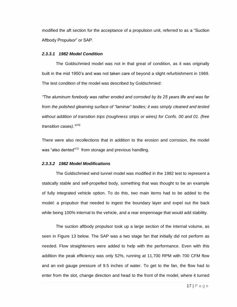
Figure 33: Pressure port locations on the aft body .......................................................... 45
Figure 34: Lip on the aft section of the wind tunnel model .............................................. 46
Figure 35: Final slot geometry with cusp A and aft lip modeled ...................................... 46
Figure 36: Final body geometry with Cusp A and 0.385" slot gap ................................... 47
Figure 37: Freestream geometry ...................................................................................... 48
Figure 38: Straight tunnel geometry ................................................................................. 48
Figure 39: Tunnel with contraction geometry ................................................................... 49
Figure 40: C-mesh around the freestream body geometry .............................................. 51
Figure 41: H-mesh around the tunnel body geometry ..................................................... 51
Figure 42: H-grid showing the nose corner meshing ....................................................... 52
Figure 43: Aft section with slot grid meshing .................................................................... 53
Figure 44: A close view of slot inlet meshing technique .................................................. 54
Figure 45: Freestream final mesh..................................................................................... 55
Figure 46: Straight tunnel final mesh ................................................................................ 55
Figure 47: Contraction final mesh..................................................................................... 56
Figure 48: Body Y+ values for fan off case ...................................................................... 57
Figure 49: Body Y+ values for fan on with a ΔP of 1500 Pascals ................................... 58
Figure 50: Grid indepence for fan off conditions using the GCI method ......................... 60
Figure 51: Grid indepence check for fan on (500 pa) conditions using the GCI
method ............................................................................................................ 60
Figure 52: Visual comparison of near wall treatment methods (27) ................................... 71
Figure 53: Zones in a typical incompressible turbulent boundary layer (26) ...................... 71

xii
Figure 54: Contours of static pressure across the fan with a pressure increase of
500 pascals ..................................................................................................... 73
Figure 55: Velocity contours (m/s) for fan off and fan on at 500 pascals ........................ 79
Figure 56: Pressure contours (pascals) for fan off and fan on at 500 pascals ................ 80
Figure 57: Streamlines colored by velocity (m/s) for fan off and fan on at 500
pascals ............................................................................................................ 81
Figure 58: Close up rear streamlines colored by velocity (m/s) for fan off and fan
on at 500 pascals ............................................................................................ 82
Figure 59: Inlet streamlines colored by velocity (m/s) for fan on at 500 pascals ............. 83
Figure 60: Velocity contours (m/s) for straight tunnel geometry ...................................... 84
Figure 61: Velocity contours (m/s) for tunnel contraction geometry ................................ 84
Figure 62: Tunnel effects on body Cp for fan off conditions ............................................ 85
Figure 63: Tunnel effects on body Cp for fan on at 500 pascals ..................................... 85
Figure 64: Straight tunnel wall Cp .................................................................................... 87
Figure 65: Cp disribution for fan pressures of 0 to 1500 Pascals .................................... 89
Figure 66: Cp vs. R2 values for varying fan pressures ..................................................... 90
Figure 67: CFD Body axial force build-up for different fan speeds .................................. 92
Figure 68: Breakup of body sections between the fore, aft, and slot sectons ................. 92
Figure 69: CFD Total force build-up for different fan speeds........................................... 93
Figure 70: Velocity vector plots showing the flow at the inlet entrance for varying
fan speeds ....................................................................................................... 94
Figure 71: Pressure drag coefficents for different turbulence models at different
fan pressures .................................................................................................. 96
Figure 72: Comparison of Cp CFD data to Cal Poly experimental data for fan off
conditions ........................................................................................................ 98
Figure 73: Comparison of Cp CFD data to Cal Poly experimental data for the fan
at 300 Pa ......................................................................................................... 99
Figure 74: 3x4ft 3-D tunnel cross section static pressure contours for straight
model at 20% chord ...................................................................................... 101
Figure 75: 3x4ft 3-D tunnel cross section static pressure contours with model in 2
degrees of beta at 20% chord ...................................................................... 102
Figure 76: Correlation between Cp difference at 20% chord and side slip angle
(beta) ............................................................................................................. 102

xiii
Figure 77: Comparison of Cp CFD data to Cal Poly experimental data for all fan
conditions ...................................................................................................... 104
Figure 78: Comparison of CFD fan speeds to Cal Poly experimental data: Aft
Section .......................................................................................................... 105
Figure 79: Experimental axial force for different geometries at the 5 different fan
settings .......................................................................................................... 106
Figure 80: Flood filled velocity contours for max fan speed ........................................... 108

xiv
Nomenclature
A Area (m2)
BLC Boundary Layer Control
BLI Boundary Layer Ingestion
BLS Boundary Layer Suction
CD Total axial force Coefficient,
Cd,p Pressure Drag Coefficient,
Cd,w Wake Drag Coefficient,
Cp Pressure Coefficient,
Cq Suction Flow Coefficient
D Total axial force (N)
Dp Pressure Drag (N)
FS Factor of Safety
L Model length (m)
Mass Flow Rate, (kg/s)
p Static Pressure (Pa)
p Apparent Order of Refinement
Freestream Static Pressure (Pa)
P Total Pressure (Pa)
Q Volume Flow Rate (m3/s)
q Freestream Dynamic Pressure,
(Pa)
r Radius (m)
r Refinement Factor
ReL Reynolds Number,
T Temperature (K)
u* Friction velocity
V Velocity (m/s)

xv
Freestream Velocity Vector
for 3D: = (vx, vy,, vz) or 2D axisymmetric: = (vx, vr)
Model body volume (m3)
y+ Dimensionless wall distance
x Distance from nose (m)
x, r 2-D Asymmetrical Coordinates
x, y, z 3-D Cartesian Coordinates
Greek Characters
ρ Density
Stress Tensor
Wall shear stress
μ Dynamic Viscosity
Kinematic Viscosity μ / ρ

1 | P a g e
1 Introduction
1.1 Goldschmied Body
The motivation behind the recent Goldschmied propulsor research is to provide
knowledge on the reduction of blunt body drag by a method that combines boundary
layer suction and boundary layer ingestion for the propulsor. In the 1950’s through the
1980’s Fabio Goldschmied looked these self-propelled bodies like airships and
underwater vehicles and from his research he found a means to greatly reduce drag.
“As compared to wind-tunnel tests of conventional streamlined
bodies at exactly the same volume Reynolds number, the
integrated vehicle design requires ~50% less power for both
free-transition and tripped transition cases”
-Fabio Goldschmied describing his results from testing(1)
The vehicle uses a boundary layer suction system through a single suction slot on
the aft section to increase pressure recovery. This slow moving air is then fed into the
inlet of the propulsion system, which provides a more efficient propulsive system than a
conventional system that takes in free stream velocity. Goldschmied is credited at
combining these two technologies in a synergistic method that has the potential to
greatly decrease the power needed to move a blunt body through the air or water.
1.2 Motivation
If this idea is applied to an aircraft fuselage (2), while the overall drag reduction
would not be as large for an airship, there would still be a great reduction in drag.
Fuselage drag for most subsonic general aviation aircraft accounts for 30 to 50% of the

2 | P a g e
total zero drag of an airplane.(3) If that drag can be reduce by 50%, there would be an
overall vehicle drag reduction of 15-25%. This would be a huge finding, as current
commercial wing and tube designs typically find single percent point decreases in drag
as a great increase in drag reduction. Groups including NASA and Boeing, have placed
much more importance on drag reduction as the current growth of the airline industry is
projected to more than double in the next 20 years(4) in addition to the cost of fuel. These
groups have set metrics to drastically reduce noise and emissions along with increasing
commercial vehicle performance. These metrics include 10, 15 and 20 year goals, with
the 2020 mark being a 50% decrease in aircraft fuel/energy consumption as compared
to 2005 best in class aircraft.(5) NASA has also included a projected breakdown of where
they predict these improvements will come from. This can be seen below in Figure 1.
Figure 1: Airframe technologies to reduce fuel burn for both an advanced Tube and Wing and Hybrid Body Aircraft
(5)
This shows that for a standard wing and tube aircraft, only a 0.7% decrease in
fuel is expected. With a drastic vehicle reconfiguration, like a blended body aircraft, a
potential 15.9% decrease in fuel usage is expected. As stated earlier, Goldschmied

3 | P a g e
projected a 15 to 25% decrease in vehicle drag. This was due to the elimination of
pressure drag. When looking at Figure 2 for a standard subsonic transport, the lowest
base drag occurs at a fineness ratio of approximately 1/3 where the coefficients of
friction and pressure drag are about equal. If the pressure drag was eliminated, we
would see roughly a 50% decrease in drag(6), similar to what Goldschmied claimed.
Figure 2: Subsonic fuselage drag from skin friction and pressure drag as a function of fineness ratio
(6)
If this drag reduction could be obtained, it will have a huge impact on the aviation
industry. Two examples of this can be seen in Figure 3 and Figure 4 on the next page.
0
0.02
0.04
0.06
0.08
0.1
0.12
0 0.2 0.4 0.6 0.8 1
CD
o
d/l
CDPmin
CF
CD0

4 | P a g e
Figure 3: Schematic layout of a 2-seat GA aircraft with integrated Goldschmied Propulsor(2)
Figure 4: Comparision of a conventional airship and a Goldschmied airship(7)

5 | P a g e
This is very enticing, however, there is little information beside the handful of
wind tunnel tests that Goldschmied and Cerreta have conducted to support this finding.(1)
(7)(8)(9)(10) A lot of their test information either left questions about the geometry,
procedures, or was just not available. To evaluate Goldschmied’s claims, two graduate
students at California Polytechnic State University in San Luis Obispo have created a
wind tunnel model and computational fluid dynamics model to try to replicate the earlier
wind tunnel results.

6 | P a g e
2 Background
The idea of boundary layer control, both with suction and blowing, is nothing new.
The technology has been around since the 1920’s(11) with some of the earliest wind
tunnel testing being completed in the early 1940’s.(12) The research done has been
promising but it has yet to ‘buy’ itself onto a commercial vehicle. Goldschmied aimed to
fix this with multiple wind tunnel tests and wrote papers on the possible integration with
general aviation aircraft. This idea has yet to catch on, due partially to the mechanisms
involved, but also due to the lack of knowledge and data in the subject. The background
presented here is to show what has been done and let us pick up where Goldschmied
and others have left off, with the goal of getting a better understanding of the synergy of
boundary layer suction and ingestion.
2.1 Boundary Layer Suction and Boundary Layer Ingestion
There are two main technologies that are used on the Goldschmied Propulsor:
boundary layer suction and boundary layer ingestion. While both can offer improvements
independently of each other the real advantage for the Goldschmied Propulsor is that it
uses both technologies at once to obtain a synergistic result to give the greatest
efficiencies.
Boundary layer suction (BLS) works by removing the slow moving boundary layer
which allow for higher energy flow to come down to the surface. The BLS method results
in a thinner boundary layer that can stay attached longer. This lack of separation due to
BLS is advantageous in aircraft applications because it allows for higher lift airfoils, as
the onset of stall is extended. It also can reduce pressure drag, as the newly attached
flow can withstand a higher pressure recovery than the slower moving flow that was
removed.

7 | P a g e
Boundary later ingestion (BLI) works by ingesting the boundary layer for use in the
propulsor unit. With a BLI system, the flow is already going relatively slow upon entering
the propulsor and greater propulsive efficiency is possible because the system requires
less energy to get the same increase in momentum from the low speed flow as it would
for a higher speed flow. Ideally, if a system is able to ingest all the slow moving air
around a vehicle it will just need to speed up the flow back to freestream velocity to
counteract all drag.
The Goldschmied system uses both of these technologies to create a system that
greatly reduces the pressure drag while increasing the propulsor efficiency in one single
mechanism.
2.2 Early Wind Tunnel Testing
The earliest test of boundary layer ingestion for the reduction of pressure drag was
seen in wind tunnel testing as early as 1944 in the National Physical Laboratory in
London, England by E. Richards and W. Walker(12). The test involved a 16% thick Griffin
airfoil that spanned the width of the 9ft tunnel with a 4ft center section that was isolated
using wing plates. The airfoil had a 6ft chord and was run at a Reynolds number of
25x106. The center section housed a suction slot, pressure ports, and all of the
instrumentation. This was done to investigate the two dimensional flow and the behavior
of the slot. Although they showed that they had a better pressure recovery on the aft
section, there was not much change from the power off condition because the flow
stayed attached at all settings, including fan off. This is largely a result of the relatively
thin airfoil and the smooth long aft section that keeps the flow attached. The pressure
recovery change due to the suction can be seen in Figure 5 below.

8 | P a g e
Figure 5: Griffith airfoil with and without suction(12)
Another item they were looking at was total drag reduction, which included looking
into maintaining laminar flow for as long as possible. Initially they had many difficulties
getting a smooth geometry. The initial body had a large amount of waviness that would
trip the boundary layer and make it turbulent. They noticed that small changes could
have a large effect on the overall behavior of the flow. Their testing also included trying
to get the boundary layer to stay laminar across suction slots and continue on the aft
section. They were able to do this for a small section but because of the concavity of the
aft region along with the adverse pressure gradient they were ultimately unsuccessful. At
the end of the paper they provided ten points that summarized what they found.(12) The
most helpful points can be seen below:
(1) Backward-facing slots seem to be slightly more efficient than forward-facing slots

9 | P a g e
(2) Slot widths up to three time boundary layer thicknesses may be safely used, but
the proportion of the boundary layer absorbed increases with increase of slot
width
(3) A slot width at least equal to the laminar boundary layer thickness at the slot
should be used to prevent high frictional losses at the duct entry.
(5) With transition at any point forward of the slot, between 0.05 and 0.10 of the
turbulent boundary layer air at the slot must be absorbed to prevent separation
(as indicated by silk threads)
(8) For slot widths greater than that of a single laminar boundary layer thickness, the
suction head with minimum suction is less for forward transition than with laminar
flow to the slot.
(9) No improvement in effective drag coefficient can be obtained by causing
transition forward of the slot. On the other hand, the effect of forward movements
of transition will be no greater than for a normal low-drag wing.
(10) With forward transition, the extra suction needed to establish the non-
separated flow regime over that needed simply to maintain it, is no greater than
with laminar flow to the slot.
2.3 Goldschmied and Cerreta’s BLS and BLI Tests
As stated earlier, Fabio Goldschmied spent a lot of time and effort trying to prove
the gains from the propulsor. He was the main proponent of this technology and spent
over 30 years looking at the concept. Because of this we look to him as an expert in that
subject area, hoping to glean from his previous testing to help us move forward with
ours.

10 | P a g e
2.3.1 1956 Test
The initial testing of the Goldschmied body was run at the Aerodynamic
Laboratory at the David Taylor Model Basin. There are two main papers that
documented this test, one by Cerreta(8) that was a report to U.S. Navy and a second
done for Goodyear Aircraft Company(7). This test was initially planned to span three
months but this was greatly reduced because of budget concerns. This changed the
overall test approach from finding what combination of aft shape, slot gap, fan speeds,
and additional geometry that provided an optimal configuration to a test approach that
demonstrated what initial designs showed promise for further research.
2.3.1.1 1956 Wind Tunnel Test models
Two models were tested: the first being a XZS2G-1 Airship which was modeled
at a 1/70th scale at 58.8” and the second being the Goldschmied model that was made
from a modified Griffith/Lighthill airfoil to be the same volume as the XZS2G1. The
XZS2G-1 airship was one used as a model because it was one of the lowest drag
airships of its day, and would make a good reference point for drag comparisons. The
geometry can be seen below in Figure 6.
Figure 6: XZS2G-1 Airship used in 1956 testing(8)
The Goldschmied body being tested was setup as a proof of concept model. The
suction slot was fed by a pump that was located external to the wind tunnel. This allowed

11 | P a g e
them to solely look at the BLI on the aft body and see how that compared to the airship
model and not have to work on integrating a fan in the aft section. The geometry was
constructed from a Lighthill/Griffin Airfoil. This geometry was chosen as the maximum
thickness is farther back than most airfoils, which helps maintain laminar flow and small
boundary layers. This model was not optimized but thought to be a good enough shape
that would function as a technology demonstrator and if successful the body could later
be optimized. The model geometry can be seen below in Figure 7. There were also
three main aft configurations that were looked at. The first configuration was considered
the ‘standard’ with a straight slot and a concave aft section. The second configuration
change added a shroud around the aft section facing forward to help the flow enter the
slot. The third configuration was an annular ring that was mounted above the aft body.
The annular ring had the slot closed and was tested to see if it could replicate the effect
of the slot. All three configurations can be seen in Figure 8.
Figure 7: 1956 Original Goldschmied Test Model(10)

12 | P a g e
Figure 8: The three test configurations for the Goldschmied body (8)
2.3.1.2 1956 Test Results
Since Goldschmied & Cerreta had limited time in the wind tunnel, they only found
general trends and results, mainly setting up a starting point for future tests. From the
initial XZS2G-1 airship, Goldschmied & Cerreta saw that the Goldschmied body with fan
off had about 50% more drag. Then when the suction was turned on, the drag was
greatly reduced, going to a fraction of the initial. This drag value was added to an
estimated ‘suction drag’ that was computed to estimate the power needed by the
suction, to get the total drag. This total drag was calculated 20-30% less drag than the
XZS2G-1 airship. Another important factor discovered is that once the suction rate was
increased enough to attach the flow on the aft section, any increase after that had little to
no effect on the body’s drag. Also, the tail cone with the shroud slightly decreased the
power needed for flow attachment but no other effects after that. For the final
configuration with the annular airfoil, they found that this did not decrease the drag at all
but rather it increased it worse than the initial fan off condition without the annular airfoil.
From this Goldschmied & Cerreta concluded that the main conclusion was that the
suction kept the flow attached and reduced drag by more than 20%.

13 | P a g e
2.3.2 1969 Test
The second test of the Goldshmied body was done in 1969. During this test
Goldschmied & Cerreta resurrected the initial 1956 model and added more
measurement instruments along with an added cusp at the slot entrance. The main
paper for this test could not be located. The only information for this test was found in
later papers that referenced this 2nd test and reproduced only a small fraction of the
original plots and numbers. For reference, the original test paper was cited in a later
report(1) as: “Aerodynamic analysis of the 1969 wind-tunnel test of the Goldschmied body
Vol.I –Slot geometries and body distribution; Vol. II Boundary-layer suction, transition
and wake drag,” Westinghouse Electric Corp., R&D Center, Research Report 77-1E9-
BLCON (March 1977). The most comprehensive information was reproduced in 1978 in
Goldschmied’s body optimization paper(13), which is our main source of knowledge
concerning the 1969 test.
2.3.2.1 Modified Geometry
One of the main improvements during this test was the addition of a cusp at the
slot entrance. This cusp supposedly both decreased drag at the power off condition and
increased suction stability while decreasing needed fan power to keep the flow attached.
The best image of this cusp is seen in Figure 9. There are no coordinate points or
information about the exact geometry.

14 | P a g e
Figure 9: Clay filled cusp cross section added in the 1969 test(13)
The paper does reference that the geometry was inspired by a paper by Friedrich
Ringleb in 1961.(14) Ringleb talks about the natural formation of ice cusps on ridges due
to the air and snow circulating. As small quantities of ice get deposited, the cusp slowly
forms into a shape that helps the flow circulate around the corner. This design is
supposed to be better because, unlike a solid surface, the flow at the separating
streamline is moving, which removes a lot of the shear stresses that take energy out of
the flow. The inspiration for the cusps can be seen in Figure 10 below.
Figure 10: Ringleb scheme of a snow cornice used for cusp inspiration(14)
From the report it seems that this cusp greatly improved the performance, but there is
very little information on the actual geometry.

15 | P a g e
Finally the model was tested with a ±6° angle of attack. These tests were done to
see how the Cp changed and if the aft section was adversely affected.
Figure 11: Pressure distributions for +/-6 degree angle of attack for test model (13)
From the graph in Figure 11 we can see that the six degree angle change did not result
in drastic changes to the flow around the body. It behaved as expected, with the fore
section increasing in pressure and the aft section decreasing in pressure at six degrees
of inclination.
2.3.2.2 Results of the 1969 Testing
As stated earlier, the actual test document could not be found. Because of this
we do not have Goldschmied’s full data set or exact test conditions, rather we have a
few graphs that were reproduced in later papers by Goldschmied, this can be seen in
Figure 11 above and Figure 12 below.

16 | P a g e
Figure 12: Fan off cusp vortex effect for 1969 test(13)
From Figure 12 we see that they tested the fan off conditions and saw that the
cusp provided passive suction that helped increase the pressure recovery on the aft
section, increasing it to nearly a Cp of 0.35. There isn’t much more on this besides a
sentence or two and leaves a lot to be desired by the reader. The statement with the
most useful summary of the 1969 test was mentioned in Goldschmied’s body
optimization paper(13). In this, he states: “The best configuration yielded a drag coefficient
of CD = 0.0144 at the volume Reynolds number of R = 3.13 x 10⁶; laminar boundary-
layer flow was maintained up to ~70% body length by actual wind-tunnel China Clay
visualization.”
2.3.3 1982 Test
In 1982, Goldschmied completed his third and final test on the Goldschmied
body. This test was aimed at integrating a propulsion unit into the aft section of the body.
This had not been done previously, as an external pump had been used for the suction
slot in the last two tests. The 1982 test used the same wind tunnel model as before but
17 | P a g e
modified the aft section for the acceptance of a propulsion unit, referred to as a “Suction
Aftbody Propulsor” or SAP.
2.3.3.1 1982 Model Condition
The Goldschmied model was not in that great of condition, as it was originally
built in the mid 1950’s and was not taken care of beyond a slight refurbishment in 1969.
The test condition of the model was described by Goldschmied:
“The aluminum forebody was rather eroded and corroded by its 25 years life and was far
from the polished gleaming surface of "laminar" bodies; it was simply cleaned and tested
without addition of transition trips (roughness strips or wires) for Confs. 00 and 01. (free
transition cases).”(15)
There were also recollections that in addition to the erosion and corrosion, the model
was “also dented”(1) from storage and previous handling.
2.3.3.2 1982 Model Modifications
The Goldschmied wind tunnel model was modified in the 1982 test to represent a
statically stable and self-propelled body, something that was thought to be an example
of fully integrated vehicle option. To do this, two main items had to be added to the
model: a propulsor that needed to ingest the boundary layer and expel out the back
while being 100% internal to the vehicle, and a rear empennage that would add stability.
The suction aftbody propulsor took up a large section of the internal volume, as
seen in Figure 13 below. The SAP was a two stage fan that initially did not perform as
needed. Flow straighteners were added to help with the performance. Even with this
addition the peak efficiency was only 52%, running at 11,700 RPM with 700 CFM flow
and an exit gauge pressure of 9.5 inches of water. To get to the fan, the flow had to
enter from the slot, change direction and head to the front of the model, where it turned

18 | P a g e
around again to enter the fan inlet. This two 180° vane-less corners leading up to the fan
were noted to be inefficient and should be improved in future models.
Figure 13: Internal schematic of the suction aftbody propulsor integration(9)
Finally an empennage was added that extended out of the center of the exit slot.
The empennage extended out half the length of the original and was no larger than the
maximum diameter of the forebody. The exact geometry details were catalogued in the
1982 test report by Howe and Neumann(9). The final model with empennage can be seen
in Figure 14.

19 | P a g e
Figure 14: Fabio Goldschmied with the 1986 model and attached tail section (9)
2.3.3.3 1982 Testing Results
When collecting results, there were two methods used to calculate drag, one from
the sting and the second from a wake survey. These results were far from ideal, as the
sting was not able to accurately tare with the interference of the strut/model. The inability
to accurately tare the values causes the validity of the sting forces to be questioned. For
the wake survey, there were no azimuth measurements conducted so they were not
totally sure the readings were in the center of the wake. Additionally there were large
variations in the turbulent wake measurements, which bring up questions about the
“steady state” values.
Even with these hardships Goldschmied claims that the tests saw ~50% drag
reduction compared to that of a conventional streamlined body and that the added
empennage added the stability needed for the model to be statically stable. These
results were very similar to the results from the previous two wind tunnel tests.

20 | P a g e
Goldschmied concluded from this testing that three elements must be
incorporated in future designs to get the best efficiencies and boundary layer stabilities.
The first being a suction slot, to ingest the boundary layer. The second element is a
cusp on the inlet of the suction slot, as seen from the 1969 test. And finally a tail boom is
needed to help stabilize the flow exiting the fan.
2.4 Recent Computational Fluid Dynamic Studies
Up until recently there has been no CFD replication or validation of the
Goldschmied body. The paper “Computational Study of the Embedded Engine Static
Pressure Thrust Propulsion System” by Peraudo et al. (16) looked to provide the CFD
basis for an embedded propulsion system. They did this by replicating Cerreta and
Goldschmied’s tests as described above. All CFD cases were run in FLUENT with
structured grids of approximately one million cells. All geometries used the Grid
Convergence Index (GCI) to estimate uncertainties due to discretization error. Initial runs
looked at different turbulence models, but the k-ω SST model gave the best results, so
from here out we will be quoting those numbers.
2.4.1.1 ZXS2G-1 Airship
The first test case Peraudo et al. ran was of the ZXS2G-1 Airship test done by
Cerreta in 1957 (8). The geometry with CFD results of velocity and streamlines can be
seen in Figure 15. Overall the CFD for the airship matched well, especially with the
experimental wake profile. The drag was slightly under predicted by about 15% for this
case, with a CD,W = 0.0242 compared to the experimental of CD,W = 0.0284. The author
stated that because of coarse geometry information, the missing experimental data, and
approximations in the experimental data reduction used in the 1957 test, that 15%
differences in the solution was still in agreement overall.

21 | P a g e
Figure 15: Peraudo CFD velocity contours with k-omega SST turbulence model for the XZS2G-1 Airshrship
(16)
2.4.1.2 1969 Test Model
The next model that was tested was the initial Goldschmied body with boundary
layer ingestion, as can be seen in Figure 16. Here two cases were looked at, one with
suction off and one with suction on. The methods used were very similar to the first trial
with the main difference being the difference between the CFD and experimental fan off
drag values. The CFD gave a fan off drag value of CD,W = 0.0307, which was about a
20% increase from the ZXS2G-1 airship and the experimental value was given as CD,W =
0.0558. This seemed really high and was a lot different than the 1982 fan off test results
of CD,W = 0.0340, so it was Peraudo’s recommendation to disregard Goldschmied’s high
fan off drag values, as it seemed to be either a typo or anomaly. The fan on values are
close to the experimental values, with CFD value of 0.0053 and the experimental value
0.0052.

22 | P a g e
Figure 16: Medium mesh for the 1969 un-propelled Goldschmied model(16)
2.4.1.3 1982 Test Model
The 1982 model was of the most interest because it contained the complicated
internal flow, along with the boundary layer suction, the exit jet, and the interactions
between all of the components. The structured grid, along with the fan on streamlines,
can be seen in Figure 17 and Figure 18 below. One interesting note is that the internal
geometry was not taken from Howe’s test procedure (as can be seen in Figure 13) but
from a smaller image reproduced in a paper by Goldschmied(15). This shows the difficulty
associated with trying to reproduce Goldschmied’s data and the lack of information that
was supplied from his testing. The aft section and slot geometry also seemed to differ
slightly between sources.

23 | P a g e
Figure 17: Medium structured mesh for the 1982 Goldschmied model (16)
Figure 18: Velocity contour and streamlines for the propelled airship with attached flow(16)
For this model, three cases were run: a “fan off” and two fan on cases with
varying suction rates. All three pressure distributions are shown in Figure 19 below and
can be compared to Goldschmied’s experimental results.

24 | P a g e
Figure 19: Peraudo CFD (a) and experimental (b) Cp Distributions for the self-propelled BLC Airship with and without suction
(16)
We can see that the Cp values for the fan off condition seemed to match up pretty
well, decreasing to about Cp = -0.4 at the maximum diameter and then increasing to
about 0.1 for the separated region. The first fan on case with CQ of 0.012 was not
enough to get the flow attached in the CFD like it showed in the experimental. The flow
rate was increased until there was attachment on the aftbody. This wasn’t reached until
the flow rate was increased to 0.018, 50% higher than the experimental value. This may
have been due to the inaccuracies of modeling the slot and internal geometry or a poor
flow rate measurement by Goldschmied. Regardless of the difference in flow rates, it
seemed that in both the experimental and CFD cases, as the fan speed increased
enough to attach the flow over the aft section, the overall drag decreased to zero. A
summary of the results can be seen in Table 1.

25 | P a g e
Table 1: Peraudo CFD results for the propelled BLC model
CQ5 U5/U∞ H5/H∞ CD, Wake
Goldschmied Experimental
0 - - 0.034
0.012 0.675 0.990 0.000
CFD Results
0 - - 0.030
0.012 0.712 0.993 0.023
0.018 1.042 1.020 0.000
Overall Peraudo et al. concluded that the embedded propulsor was not optimally
designed and a good amount of improvements could be made by making that section of
the model better. There were large uncertainties in the testing results that made it hard
to compare to. Either better knowledge of the wind tunnel model and more accurate data
collection was needed or an improved model needed for testing to get more accurate
results.

26 | P a g e
3 Cal Poly’s Goldschmied Model and Testing
Over the past two years students Joshua Roepke and Nicole Thomason, from
California Polytechnic State University, San Luis Obispo CA have constructed and
tested a new Goldschmied propulsor in Cal Poly’s 3x4ft low-speed indraft wind tunnel.
The goal of the recent model and testing was to replicate Goldschmied’s results and
provide a transparent basis of knowledge for future study. The following sections
summarize what Roepke and Thomason have done; for all details the reader is
encouraged to read their theses, they can be found in references (17) and (18).
3.1 Cal Poly’s 3x4ft Wind Tunnel
All testing for the New Goldschmied body was done in Cal Poly’s 3x4ft indraft
tunnel. The tunnel was constructed in 1974 and is mostly made from wood. It is powered
by a 150 hp, 440 Volt three-phase motor that is connected to a nine-blade axial fan. A
planform view of the tunnel can be seen in Figure 20 below.
Figure 20: Top View of Cal Poly’s 3x4ft Draw Down Wind Tunnel
An important note about the tunnel was that the center test sections were all of
equal and constant area for the whole center section. There is no increase in area, as is
sometimes done by reducing the chamfers in the corners. The constant area does not

27 | P a g e
account for boundary layer growth that will effectively reduce the cross section of the
tunnel. With this reduction the average velocity in the center of the tunnel will accelerate
as it flows further downstream.
3.1.1 Recent Tunnel Modifications
Recently Cal Poly’s wind tunnel went through an inlet screen replacement that
greatly improved the flow in the test section. Greg Altmanns’s wind tunnel test (19),
previous to any of the Goldschmied testing, found that they were getting results that
were not what they expected. The problem was traced to a dirty and poorly sized inlet
screen. This was easily seen when Altmann and Roepke conducted a flow visualization
of the inlet. There were places where the inlet was nearly 100% blocked, leading to
dramatic changes in flow direction, as seen in Figure 21.
Figure 21: Wind tunnel inlet flow visualization before screen redesign(19)
This discovery led them to take apart the tunnel inlet, replace the poorly sized
screens, cleaned the other screens and the rest of the inlet. The cleaning and redesign
greatly improved the flow quality in of the inlet. The improved flow can be seen in Figure
22.

28 | P a g e
Figure 22: Wind tunnel inlet flow visualization after screen redesign (19)
After the new inlet was completed, a group of students completed a study of the
flow quality(20) at the center of the test section to find the velocity variation and
turbulence intensity. They constructed a traverse that could travel in a vertical and
horizontal direction to span the whole wind tunnel at a single station. From this they
found that the total velocity variation was about 3% off the average velocity and a
turbulence intensity of about 0.5% with a peak of about 2.7% at the top of the tunnel.
The velocity and turbulence plots can be seen in Figure 23 and Figure 24. This
discrepancy at the top seemed odd, but the data was reproduced weeks later when they
re-evaluated the tunnel. The source of this anomaly is unknown, but since it is located
near the top of the tunnel and not in the center of the test section we will assume that the
overall average turbulence for our CFD calculations will be 0.5%.

29 | P a g e
Figure 23: Velocity deviation in the improved Cal Poly wind tunnel course grid (20)
Figure 24: Cal Poly wind tunnel course grid turbulent intensity plot (20)

30 | P a g e
The blank spots in the figures above are sections that were not traversed in the course
data collection stage; rather they were saved for the fine traverse. The fine traverses are
not reproduced here, as there is no new information in them.
3.2 Cal Poly Goldschmied Model
Cal Poly’s Goldschmied propulsor was designed to replicate Goldschmied’s model with
the least amount of changes to the outer body but to also improve the internal fan unit.
The model had to be scaled down from the original 58”length and 20” diameter to
something smaller that would fit in Cal Poly’s 3x4ft tunnel. Because of the smaller tunnel
size the model was reduced so the maximum cross sectional area of the model was 9%
of the tunnel cross sectional area. This was done to keep blockage effects down to a
minimum, which was set at a maximum of a 5% increase in airspeed around the model.
This sized the maximum diameter of the model to be 13.5” and a length of 38.5”. A
comparison of this to previous models can be seen in Table 2 below.

31 | P a g e
Table 2. Summary of the original Goldschmied models compared to Cal Poly’s model(17)
1956 Model 1982 Model Cal Poly’s Model
short Long
Reynolds numbers (based on length)
4x10⁶ - 12x106 3.2 x10⁶ – 5.0 x10⁶
1.34x10⁶ (at 20 m/s)
Tunnel Size 7’ x 10’ 8’ x 10’ 3’ x 4’
Length 58.8” 54.45” / 57.17 38.5”
Maximum Diameter 20.0” 20.0” 13.5”
Location of Maximum Diameter
54.1% 57.9% / 55.1% 55.1% (21.23” from LE)
Forbody Diameter at Slot 11.5” 11.5” 7.75”
Aftbody Diameter at Slot 9.62” 9.35” 7.00”
Exit Diameter - 3.3” 1.82”
Slot Location 86% 90% / 85.8% 86% (33.12” from LE)
Body Volume Not Available 6.35 ft3 1.89 ft3
The individual subsets of the model will be talked about in the following sections, but the
final SolidWorks model can be seen in Figure 25.

32 | P a g e
Figure 25: Final Goldschmied SolidWorks Model
3.2.1 Outer Geometry
Cal Poly’s model was based on Goldschmied’s data. The main problem with this
approach was the lack of an exact set of coordinates. The geometry is based on the
locations of the pressure ports listed in each of the test papers. These values were not
exactly the same and the aft section varied between tests. The data points can be seen
below in Figure 26.
For the forebody, it was observed that its geometry is reported as nearly the
same for all tests, as the same physical model was used for all tests. These values were
averaged to find the current fore body. For the aft body, the longer of the open aft bodies

33 | P a g e
was chosen. This was chosen because it was both easier for Goldschmied to get aft
body attachment and seemed easier to mount the ducted fan and motor internally.
Figure 26: Comparison of body shapes used in Goldschmied's testing non-dimensionalized by forebody length
(7) (9)(10) (21)
These points were then reduced and smoothed out to get a shape that was both
representative of Goldschmied’s tests and would eliminate any discontinuities or bumps.
Roepke and Thomason’s theses contain more detail on their geometry selection and
refinement.
3.2.2 Slot Design and Construction
The slot is the most important feature, yet it seemed to be the least documented
geometry in the whole model. There were no values for the slot besides the outer
opening, and even that was based on simple measurements, mainly just the slot width
and inlet diameter with nothing documented about the exact routing. This made
reproducing the inlet and exit somewhat of an unknown, and most of the information was
found in drawings from the original models, as can be seen in figures on pages 11, 12,
14, 18, and 19 of this report.
With this lack of knowledge and with suggestions that the original slot was less
than ideal, the slot for the new model underwent a total redesign. The aft section was
mounted on a horizontal traverse that allowed the slot gap to vary in width. There was a
variable cusp design that allowed three different geometries to be tested. Inside the slot,
0 0.05
0.1 0.15
0.2 0.25
0 0.2 0.4 0.6 0.8 1 1.2
r/L f
b
x/Lfb

34 | P a g e
the front face was concave in to allow a constant radial cross sectional area as the flow
moved in. The motor was mounted internally to the aft section and the torque and force
were measured through a set of sensors.
3.2.2.1 Cusp Design
At the end of both the 1969 and 1982 tests, Goldschmied claimed that an added
‘Ringleb’ cusp added a huge increase in performance and helped to stabilize the flow.
Because the initial ring was formed by molding clay around the suction slot inlet by hand,
the exact geometry is not known. Understanding this, the closest reproduction of a cusp
drawing is seen in Figure 9 on page 14 above. From Thomason’s thesis, we see that
there were three main cusp geometries tested on the Cal Poly model. Cusp B, the center
of in Figure 27 below, was taken directly from Goldschmied’s original sketch.
Figure 27: Three cusp geometries that were constructed for the Goldschmied propulsor(18)
The other two cusps were variations of the first one, with Cusp A protruding less
into the flow and Cusp C protruding a lot further and turning a lot more. The goal with
these cusps was to get a basis of what worked and what didn’t and hopefully give an
idea on how to move forward in the future.
A C B

35 | P a g e
3.2.2.2 Fan Unit
The goal of the fan unit for the new model was to find something that was small
enough to fit into the aft section of the model and still be able to deliver enough suction
and flow rate to ingest enough of the boundary layer to re-attach the flow on the aft
section of the body. Having the fan mounted in the aft section got around the big losses
in Goldschmied’s original testing with his 180° turns. Also the motor was highly
monitored, to determine how much power was really needed to attach the flow. The
power supply was able to output the voltage and current that it was supplying. In
addition, the model was fitted with load cells on the aft to measure force and torque.
These measurements allowed one to measure the power delivered to the air, the power
delivered to the motor and speed controller, and thus the efficiency of the whole system.
The fan module can be seen below in Figure 28. The fan unit was capable of delivering
around 500 watts at its maximum setting.
Figure 28: Ducted fan propulsion unit and inlet rear face mounting
3.2.3 Tunnel Mounting Method
The mounting for the Cal Poly Goldschmied body did not use the standard 3x4 ft
tunnel sting, this was excluded because the sting was located at the rear of the tunnel
and for testing Roepke and Thomason wanted the cleanest air possible, which was soon

36 | P a g e
after the contraction. Also the sting was not strong enough to support the full weight of
the 38” model. With these considerations, it was decided to mount the model at the front
of the tunnel on a vertical steel bar that was allowed to rotate at the base through the
means of two flexure joints. The flexure joints allows for a friction free way to rotate,
which, when coupled with a load cell at the base, allowed one to measure the axial force
on the model.
3.2.4 Propulsor Construction
The main body of Cal Poly’s Goldschmied propulsor was made out of carbon fiber,
which was made from laying-up in a female mold. This process allowed a relatively
complex shape that would be light, stiff, and had a lot of internal space to allow for
mounting of components. A similar process was used to mold the aft body. A majority of
the rest of the components were machined out of an aluminum billet. This was because
it was light, easy to machine, and allowed for easy integration into the vehicle. An
example of this was with the cusps: they were machined out of a single piece that
allowed the cusps to be mounted to the back section of the fore body by means of a slot
and tabs that can be inserted and then rotated to secure it.
3.3 Testing Results
The testing from Roepke and Thomason’s research was run in multiple stints over
the 2011-2012 school year. The model was brought in and out of the tunnel a few times
so the wind tunnel could be used by classes during the year. The initial testing was used
to set up and run the model. Throughout the testing there were many changes to
improve the data quality and we are mainly concerned with the latest data set collected
in March. This is the data that will be directly compared to the CFD calculations.

37 | P a g e
3.3.1 Operating Conditions
Cal Poly is located in San Luis Obispo, CA, at an altitude of approximately 300ft
MSL and about 12 miles from the coast. Because of this, the wind tunnel sees very
temperate and consistent atmospheric values. The actual test values were very close to
standard sea level (SSL) operating conditions so SSL conditions are assumed. The SSL
values can be seen in Table 3. Actual test temperatures fluctuated between 56 to 61° F,
a density around 0.00235 slugs/ft3, and a pressure around 14.72psi.
Table 3: Standard Sea Level operating conditions(22)
Pressure 101.3 kPa 14.7 psi
Density 1.22 kg/m3 0.00237 slugs/ft3
Temperature 15° C 59° F
Gas Constant 287 J/kg-K 1716 ft-lbf/slug-°R
Kinematic Viscosity 1.46e-5 m2/s 1.58e-4 ft2/s
3.3.2 Thomason’s Results for 30m/s Testing
The data presented in Thomason’s thesis “Experimental Investigation of Suction
Slot Geometry on a Goldschmied Propulsor” was all run at 30m/s. It was found out later,
and described in the next section, that at this tunnel speed the propulsion unit was not
able to inhale enough of the boundary layer to fully reattach the aft section. This can be
seen in Figure 29 where there is partial attachment, but the flow is still chaotic and there
are gaps in the plow, indicating recirculation pockets.

38 | P a g e
Figure 29: Flow visualization with Cusp C and fan at full power showing separation
Thomason also concluded at the end of her thesis, “The errors [bars] make it clear that
between the different cusps and different fan speeds, there is no meaningful difference
in the pressure drag. Figure 68 [in her report] suggests that adding a cusp to the suction
slot creates no meaningful reduction in drag.” From these results, we are not going to be
comparing CFD to the 30 m/s results, as they all seemed to be separated and showing
very little changes between settings.
3.3.3 March Re-Testing at 20m/s
In March 2012, the new model was set up again, and this time tufts were added
to the model. The tufts allowed us to see at what fan setting allowed for reattachment of
the aft section. From this testing it was found that the tunnel speed had to be slowed to
20m/s to guarantee full attachment for the fastest fan speeds. This was reassuring
knowing that the data being collected was capturing the re-attachment of the flow over
the aft section, as intended. Because of this reattachment, the pressure recovery on the
aft section had greatly improved, which can be seen in Figure 30 below. This data set

39 | P a g e
captures the fan ranges that contain the flow characteristics that we are looking for. This
will be the data with which the CFD modeling will be compared. It should also be noted
that this paper is not going to reproduce all of Roepke’s results, as those can be found in
his final thesis.
Figure 30: Experimental results from the March 20m/s re-testing
-0.6
-0.4
-0.2
-1E-15
0.2
0.4
0.6
0.8
1
0 0.1 0.2 0.3 0.4 0.5 0.6 0.7 0.8 0.9 1
Cp
Body Length (x/L)
Cusp A, Slot 0.385", 0 Watts Cusp A, Slot 0.385", 100 Watts Cusp A, Slot 0.385", 200 Watts Cusp A, Slot 0.385", 300 Watts Cusp A, Slot 0.385", 400 Watts Cusp A, Slot 0.385", 500 Watts

40 | P a g e
4 Computational Fluid Dynamics Approach
The computational fluid dynamics goal was to see if/how well FLUENT, a
commercial CFD software application, is able to capture the flow around a Goldschmied
body. Because of this learning process, it took a lot of iterations to come to a finalized
model. It entailed many loops of setting up the geometry, creating a mesh, and then
solving to see what worked and what didn’t. Because of this it was a highly iterative
process, starting at a really simple model that used many default settings that eventually
evolved into a more sophisticated model and with modified settings. All of this was done
with the goal of trying to get the most accurate solution. The final CFD model was a
simplified axisymmetric model that included important features from the real model while
excluding smaller features.
4.1 Model Component Simplifications
Initial geometry models were very simple, starting with the outer mold line and a
small inlet and outlet for the fan. The first models did not model the flow as it traversed
the internal section. As the model iterated, components were added as their importance
became apparent. At the end of the process, the axisymmetric model included the outer
mold line, an accurate slot geometry including the intricate cusp shape and back wall,
fan body, motor, and exit geometry. The main components that were not modeled were
geometries that could not be modeled in a “2-D” axisymmetric case. These geometries
are described in more detail in the following section.
4.2 Axisymmetric Model
A 3-D model was considered, as it would allow for greater detail that an
axisymmetric model could not capture. These details include modeling strut interaction,
aft body mounting bolts, fan mounts, rear pressure tubing, temperature gauges in the

41 | P a g e
flow, wires, and other small items that were in the real model that could not be modeled
in an axisymmetric case. These details seemed small, as they are mostly all internal,
compared to the larger effects to be found and would not be worth the extra time need to
grid and solve a fill 3-D solution. So an axisymmetric model was used. It was hoped that
this would produce results comparable to the experiment and if it was found out after
initial test cases that this could not adequately model the flow, then a 3-D model would
be considered.
4.2.1 Axisymmetric Tunnel Simulation
Initial CFD runs showed that using an axisymmetric freestream model did not
match up to experimental data as well as hoped. The first thought was that wind tunnel
walls and set-up was the main reason for this difference. To understand the difference
better, a simple axisymmetric wind tunnel was constructed around the CFD model. This
was done because it was relatively simple to modify the grid and outer boundary
conditions to simulate wind tunnel walls. The initial wind tunnel CFD model was modeled
as a straight tunnel. The length of the section in front of the model was determined to
have the same boundary layer thickness as to what is in the wind tunnel.
When looking at the mounting of the physical model in the 3x4ft wind tunnel it was
noted that the nose of the model was nearly at the exit of the contraction. Observing this,
it was questioned what effect the model being that close to the contraction was. Because
of this it was decided that a preliminary model of the wind tunnel would be constructed
and ran. It was then compared to the straight tunnel to see how the contraction changed
the flow. More details of this can be seen in section 8.3.2, Tunnel Effects.

42 | P a g e
5 Computational Model Geometry Generation
The computational geometry used for solving needed to be as accurate as possible
to the real model if it were to replicate the results. Significant effort was put forth to find
the best and most accurate geometry. The following sections describe this effort.
5.1 Geometry Sources
The final geometry came from a few different sources: point files, SolidWorks solid
model, and the actual model. The next sections categorize what components came from
what source and how they were integrated together.
5.1.1 Point Files
The outer geometry was created from a combination of sources, as seen in
section 3.2.1. The final smooth geometry came out to a set of about 30 data points,
these data points were then used to create the solid model which led to the real model.
Since there was no good way to measure the exact geometry of the real model, it was
decided to use the set of 30 data points and create the CFD geometry around this.
5.1.2 Solid Model
The SolidWorks solid model was used for a majority of the internal slot geometry
modeling. This was because it was easier than measuring the real model and since a
majority of the components where machined from the solid model, the differences were
expected to be small. Figure 31 shows the solid model that was used, the connection
ring and cusp are hidden for simplicity.

43 | P a g e
Figure 31: SolidWorks model used to model the internal slot geometry
Using the solid model did not come without issue, as the solid model was not
exactly reproduced in the actual wind tunnel model. This can be seen in Figure 32,
where the connection ring in the solid model is not precisely tangent to the fore body and
is also not exactly aligned with the cusp. This was not the case in the real model, as the
cusp and connection ring were closer to the same size and wax was used to fill in any
non-tangent section. The solution to this was to not follow the exact SolidWorks
geometry, but to create smoother geometry that more accurately represented the
smoothed out section on the real model.

44 | P a g e
Figure 32: Discrepancies between the solid model connection ring and cusp and the final wind tunnel model
SolidWorks was also used to find the pressure port locations on the fore body. This was
the most accurate method besides actually measuring them. Comparing the SolidWorks
model to measurements of the actual model, the locations of the fore pressure ports
match up well and are in agreement.
5.1.3 Physical Cal Poly Model
Finally the physical model was consulted to find any discrepancies between the
previous methods described and the actual model that was being run in the tunnel.
A similar method in SolidWorks was used to find the fore body pressure ports, as
described above, was used to locate the pressure ports on the aft body. This gave
locations that did not seem correct. To fix this, a thin piece of foam was cut to fit the aft
body geometry and then the pressure ports were located. The fitted piece can be seen in
Figure 33 below. This was then brought onto the computer and a plot digitizer was used
to find the exact location of each port.
45 | P a g e
Figure 33: Pressure port locations on the aft body
After further inspection of the physical model it was found that there was a small
0.035” lip at the start of the aft body immediately after the slot. This discovery can be
seen below in Figure 34. This was a result of the carbon fiber aft body being slightly
larger than the aluminum ring that it mounted to. The lip was not present the whole
circumference, but it protruded for a large section that was centered around the pressure
ports. This was a very important part of the model and any small change had a large
effect on the flow on the aft body, so it was decided to add this small protrusion to the
CFD model.

46 | P a g e
Figure 34: Lip on the aft section of the wind tunnel model
The final close-up of the CFD slot entrance, with cusp A and the lip modeled can be
seen in Figure 35 below.
Figure 35: Final slot geometry with cusp A and aft lip modeled
5.2 Final Geometry
Putting all these three sources together, we get the final model geometry, as seen
below in Figure 36. The final coordinate points can be found Appendix A
0.035” (~1/32 inch)
Lip
Aftbody
Forebody Cusp A

47 | P a g e
Figure 36: Final body geometry with Cusp A and 0.385" slot gap
5.3 Boundary Geometry
There were three boundary geometries; a freestream “free-air” condition, a straight
tunnel, and a tunnel with the contraction modeled. All three were created to test different
questions about the body pressure distribution that came up in the initial CFD test runs.
5.3.1 Freestream Geometry
The freestream boundary was the first geometry created and it was made for a
standard C-grid. It extended 5 chord lengths forward, 5 above, and 10 behind the
vehicle. These values were chosen as they represent normal convention for a body that
has a relatively small effect on the surrounding flow field. The outline of this can be seen
below in Figure 37.

48 | P a g e
Figure 37: Freestream geometry
5.3.2 Straight Tunnel Geometry
After the initial CFD test cases it was decided to look to see if there was much of
a difference between the freestream conditions and tunnel geometry that the tunnel
corrections were not capturing. This was determined after looking at the change in Cp
along the body due to buoyancy and other effects. The tunnel was modeled as an
axisymmetric tunnel with the same cross sectional area. This was done to maintain the
simplicity of the axisymmetric case, but to allow for blockage, buoyancy, and other
tunnel effects. The inlet length was sized to give the same boundary layer thickness at
the test model as measured in previous tests (see section 3.1.1). This has been done in
other CFD cases(16), and is a common practice to give accurate results. The aft section
was then carried 10 chord lengths downstream to match the freestream test case. The
tunnel boundary can be seen in Figure 38 below.
Figure 38: Straight tunnel geometry

49 | P a g e
5.3.3 Tunnel with Contraction
Finally after looking at the physical model in the wind tunnel, it was observed that
the model was placed so that the nose was at the end of the contraction. It was thought
of at one point that, even as the tunnel is straight after that point, the flow still might have
some radial velocity that hasn’t been fully dissipated. Because of this the tunnel
contraction was then modeled. Like the straight tunnel, the contraction was modeled as
an axisymmetric model with the same cross sectional area as the real tunnel and the
Goldschmied body was placed in the same location as it was in the tests. This can be
seen in Figure 39 below.
Figure 39: Tunnel with contraction geometry

50 | P a g e
6 Computational Mesh
The next step in the process going from the geometry file to a solution was to create
a computational grid. The governing equations are discretized on this grid, and that
process will be discussed in more detail in section 7.1. The mesh is one of the most
important parts of computational fluid dynamics and can have a huge effect on the
solution if not done correctly. It must break the field up into small enough sections to
accurately capture the flow field, but also not too much that it requires too much
computational effort to solve.
6.1 Goldschmied Mesh Generation
The Goldschmied propulsor had 3 different geometries that were modeled and
gridded. It was decided early on that a structured mesh would be used for all the
geometries. This was done for a few reasons, one being experience of the author had
with structured grid generation versus unstructured generation. It was determined that it
was easier to spend a little more effort getting a good structured grid than it was to
stumble through the processes of making an unstructured grid.
The structured grid allowed for tighter control of important sections in the model,
like the boundary layer, the slot entrance and cusp, and finally the curved streamlines
around the aft section of the body. Also, the computational time needed to solve a
structured grid is faster than an unstructured grid. This was not too much of a concern,
as the mesh was relatively small and would not make too much difference.
6.1.1 Body Grid
The body grid was the first and most important part considered. The grid was
held as constant as possible throughout the tunnel geometry changes. This was most
important in the aft section where we were the most concerned with the flow and how

51 | P a g e
the changes effect the flow there. The largest difference between the tests was that the
free stream flow used a structured C-mesh that wrapped around the nose of the body,
and the tunnel meshed used an H-mesh to model the flow around the body. These
methods were nearly identical to the flow around the body except for the small section in
the front. The C-mesh wrapped around the nose, whereas the H-mesh continued down
the length of the tunnel. These two meshes can be seen in Figure 40 and Figure 41.
Figure 40: C-mesh around the freestream body geometry
Figure 41: H-mesh around the tunnel body geometry

52 | P a g e
When looking at the nose of the body, it was obserbed the C-grid simply wraps
around the nose and there are no issues with cells being skewed or stretching the grid
around a corner. This was not the case with the H-grid, as it comes down to the nose, it
had to manage roughly a 70° corner to go from the body to horizontally down the tunnel.
After an initial mesh, as can be seen in Figure 42, we see that this was easily handed
and the cell skewness was not too extreme and was not of concern.
Figure 42: H-grid showing the nose corner meshing
6.1.1.1 Aft Section and Internal Slot Meshing
The next section of concern for modeling was the slot geometry and how that
was to be completed. The main grid was run across the slot and then down the aft body
where it then left nearly horizontal and continued out to the farfield exit. This approach
allowed the grid to closely follow the streamlines when the flow was attached and give
the best solutions.

53 | P a g e
To model the slot, a section of the structured grid was added to the part that
spanned the slot. This was then brought down through the slot, turned as the flow does
into the fan, and then brought out the back of the body, parallel to the aft body and
continued out horizontally to the farfield exit. This can be seen below in Figure 43.
Figure 43: Aft section with slot grid meshing
This was not too difficult to implement and seemed to follow the flow through the slot
really well. It also was flexible enough to capture the internal details, like the nose cone
for the ducted fan, the step outlet, and most importantly the cusp and inlet geometry, as
described in the next section.
6.1.1.2 Cusp and Inlet Meshing
The inlet was the most challenging part of the geometry to accurately capture. After a
few trials, it was possible to mesh and make the geometry fit as needed. The geometry
can be seen below in Figure 44.

54 | P a g e
Figure 44: A close view of slot inlet meshing technique
Here the outer grid was snaked to span the gap and continue on the aft section of the
model. From there the snaked section was extended further down to capture the lip at
the aft section of the slot. This was then rotated and brought down to the slot entrance.
This was feasible because the corners were rounded and allowed for the grid to rotate
around the corner without any issues.
6.1.2 Tunnel Modeling
After the body was modeled, the grid was continued out until it reached the outer
boundary walls. For the freestream conditions this was easily done and can be seen in
Figure 45. It should be noted that although it looked like an extremely fast cell size
change from the near body to the far body, this is not the case. All cell growth in the field
was mostly 1.05 and never more than 1.1. The dark regions are because of the lack of
resolution of the images.

55 | P a g e
Figure 45: Freestream final mesh
The next piece to be modeled was the straight tunnel section. This was also relatively
simple, as the mesh was brought up and then forward and back to the boundary
conditions. The only difference here was the wall was modeled on the top section of the
mesh. This modeling required the cells to be closely clustered at the wall to catch the
viscous effects of the boundary layer. This can be seen in Figure 46.
Figure 46: Straight tunnel final mesh
The last case to be modeled was the tunnel with the contraction. As described earlier,
this was modeled using the same cross sectional area as the real tunnel with the body
placed at the same location. This was similar to the straight tunnel except more
consideration was put into the expansion of the grid as it left the nose of the model and
continued out to the inlet of the tunnel. The final mesh on the tunnel contraction can be
seen in Figure 47 below. The aft section of this mesh was exactly the same as the
straight tunnel section.

56 | P a g e
Figure 47: Contraction final mesh
6.2 Surface Mesh and Y+ Calculation
The surface mesh on the wall surfaces must be small enough to capture the
viscous boundary layer effects. This is really important for the turbulence model
accuracy and being able to accurately compare the boundary layer. More detail of the
needs will be described in the turbulence modeling section, but the main point is that the
flow near any solid wall should have a y+ value that corresponds to what is needed from
the turbulence model. Y+ is the dimensionless wall distance that is defined as follows(23):
( 1 )
The y+ (from our turbulence modeling) and the kinematic viscosity for the fluid are
known. The only value needed is the friction velocity (u*) to find the needed wall spacing.
The friction velocity is defined as:
( 2 )
And the wall shear stress is defined as:
( 3 )

57 | P a g e
After determining all of these values, our only unknown was the skin friction
value. This could not be computed exactly before knowing the final solution. Because of
this the skin friction value was estimated using a skin friction correlation to give us the
largest skin friction value that was likely to seen in the flow based on the body length,
operating velocity, air density, and dynamic viscosity. There are many methods available
to use, for example the 1/7th power lay, Schlichting skin-friction formula, Prandtl’s
formula, and many more. The y+ calculator used in our calculations used the Schlichting
skin-friction formula. Using the reference values, the wall distances of 1.84e-5 m and
3.07e-5 m would be for 35m/s and 20m/s freestream velocities, respectively. The wall
distance required for 35m/s was used in case the 32 m/s results were to be compared at
a later date.
Results from FLUENT show that for the fan off case, at 20 m/s, the y+ values are
always below 1. For the higher fan speeds the exit velocity is faster than the freestream
velocity and here is where we see the increase in y+. Although it does increase, the
maximum y+ is still below a value of 2, which is still fine, and far below a maximum y+ of
5. The plots for fan on and fan off can be seen Figure 48 and Figure 49 below.
Figure 48: Body Y+ values for fan off case

58 | P a g e
Figure 49: Body Y+ values for fan on with a ΔP of 1500 Pascals
6.3 Grid Independence Study
The CFD mesh is one of the single most important items in the whole solution
process. Because of its importance, it was good to double check that the flow field has
been accurately discretized and that the discretization was on a path to convergence in
the asymptotic region. To determine this, it was recommended (24) that CFD applications
have a standardized method for finding the discretization error and convergence order.
From the wide usage and well tested results, Roache’s Grid Convergence Method is the
industry standard and will be used in this paper.
6.3.1 Grid Convergence Index (GCI) Method
Using Roache’s Grid Convergence Method the grid refinement factor (r),
apparent order (p) are initially found then used to find an exact value along with the error
from the finest grid value. The exact value is found by:
( 4 )
And:

59 | P a g e
( 5 )
where and
are the values of interest from the mid and fine grids, ea is the
approximate relative error, and FS is the factor of safety.
Oberkampf and Roy(25) suggested that if the apparent order is within 10% of the
formal order then the factor of safety (Fs) should be 1.25 with the apparent order used. If
the apparent order is different than the formal order by more than 10% then a factor of
safety (Fs) of 3 should be used. Also the exact order should be used in the calculations if
the apparent order is greater.
6.3.2 GCI Results
The original gird was used with two smaller grids. A small grid refinement factor
(1.35) was chosen to keep the grid from getting too coarse. This was used from the
recommendation from Celik et al.(24) that from their experience a minimum grid
refinement factor of 1.3 or greater be used. This gave grid sizes of 126,086 and 67,234
cells from the original 230,264. The minimum size of 67,234 did not seem too small, as
where in Peraudo’s paper(16), the coarsest grids used for the suction slot geometries
were 44,032 and 83,140 cells.
Two cases were looked at for the grid independence study, one with the fan off
and a second with the fan on. The total pressure drag from the body was used as the
critical variable in the study. The three grids were run, for both cases, noting the
pressure drag. The fan off case gave an oscillatory convergence, with the middle grid
having the smallest drag value of the three grids. Because of this the apparent order was
significantly off and the error bars, as seen in the red dashed lines in Figure 50, were
relatively large. The GCI for the fan off grid was approximately 11.0% for the fine grid
value.

60 | P a g e
Figure 50: Grid indepence for fan off conditions using the GCI method
The fan on cases had better performance, with an apparent order of 1.244
compared to the formal order of 1.351, a difference of 8%. This gave a closer exact
value of CD = 0.0272 and tighter error bars, as the GCI value was 1.63% error. The can
be seen in Figure 51 below.
Figure 51: Grid indepence check for fan on (500 pa) conditions using the GCI method

61 | P a g e
The majority of cases ran were with fan on settings, so the 1.63% error will be used
in comparing the different fan on settings. When looking at comparing the fan off
settings, the 11.0% error will be used.

62 | P a g e
7 Computational Method
ANSYS’s CFD solver, FLUENT, was used for the solver and post processing for all
the simulations presented in this paper. The solver used in FLUENT uses the Reynolds-
Averaged Navier Stokes equations (RANS) to get a time averaged solution of the flow
field.
When solving, the pressure based solver in FLUENT was used. This was chosen
because the flow was moving relatively slow (mach < 0.06) and this it can be assumed
that the flow is incompressible. It makes solving the problem easier, as density does not
need to be solved for and that we do not need to solve the energy equation. If it was in
the compressible regime, a density based solver would be needed, along with solving
the energy equation.
7.1 Governing Equations
The governing equations for fluid flows are based on the principles of conservation
of mass, momentum, and energy. These equations are made up of coupled, non-linear
partial differential equations that have no general exact solutions; rather they have to be
solved numerically through a highly iterative process. The derivations of these equations
are beyond the scope of this paper and are in most modern aerodynamic textbooks(23)(26)
and classes. What is presented here is based on the description that FLUENT presents
in its theory guide.(27)
7.1.1 Continuity Equation
FLUENT has the conservation of mass written as:
( 6 )

63 | P a g e
where the additional Sm term account for phase change, like in evaporation, or for any
user-defined sources. For most cases this is set to zero and we then get the standard
continuity equation. Because our cases are 2D axisymmetric, we would like to note that
the continuity equation is changed into polar coordinates; x and r
( 7 )
7.1.2 Momentum Equation
Conservation of momentum in a non-accelerating inertial reference frame can be
described as
( 8 )
where p is the static pressure, and are the gravitational and external forces, and
finally is the stress tensor. Which can be given by
( 9 )
where μ is the molecular viscosity, I is the unit tensor.
The momentum equation is modified slightly for 2D axisymmetric cases, the axial
and radial equations are given below.
( 10 )
and

64 | P a g e
( 11 )
where
( 12 )
7.1.3 Energy Equation
The energy equation can be written as
( 13 )
the three bracketed terms on the right hand side of the equation are the energy transfer
due to conduction, species diffusion, and viscous dissipation.
We have included the energy for good measure but it was not used. The energy
equation did not need to be solved as we used a pressure based solver, no heat transfer
was assumed, and that heat generation due to viscous effects was negligible. Also our
flow was quite slow (~mach 0.06) so no compressibility effects are seen and the density
can be assumed to be constant.
7.2 Turbulence Modeling
When using the Reynolds-Averaged Navier Stokes equations, there is one term in
the momentum equation, the Turbulent-Shear also known as the Reynolds-Stress Term:
, that cannot be calculated directly from known values. Because we are not able
to calculate the turbulent term directly, turbulence models are used to approximate these
values. The following sections show the process of modeling this turbulence term,
highlighting the turbulence models that FLUENT uses.

65 | P a g e
It should be noted that direct numerical simulation (DNS) can calculate these
values, but it is highly computationally expensive. Because of this DNS is only used on
geometric simple problems and low Reynolds number flows.
7.2.1 Boussinesq Hypothesis
The Boussinesq hypothesis is used in turbulence models like the Sparlart-
Allmaras, k-ε, and k-ω models and is how these models relate the Reynolds stresses to
the mean velocity gradients. Here it assumes that the turbulent viscosity is an isotropic
scalar quantity, which isn’t exactly true but is a good approximation for most flows. The
form of the Boussinesq approximation that FLUENT uses is shown below:
( 14 )
All of these terms are known except the turbulent viscosity, , this is the term to be
computed by the first three turbulence models described below. Once the turbulent
viscosity is found, it is plugged into the Boussineq approximation and the Reynolds
stresses are found.
Higher order solutions, like the transition and Reynolds stress models, do not use
the Boussinesq approximation. They do not assume that the turbulent viscosity is
isotropic, which plays a role in highly swirling flows and stress-driven secondary flows.
With this detail additional equations are needed to compute the flow, five for 2D and
seven more for 3D flows.
7.2.2 Sparlart – Allmaras
The Sparlart-Allmaras is the simplest model offered by FLUENT that takes into
account turbulent flows (as opposed to inviscid and laminar models). The Sparlart-
Allmaras model is a one equation model, which means it used one more partial

66 | P a g e
differential equation to solve for the Reynolds stress term. It is a turbulence model that
was developed for the aerospace industry and has shown good results for boundary
layers subjected to adverse pressure gradients. While good at boundary layer flows, the
Sparlart-Allmaras model has shortcomings with general industrial flows, like free shear
flows including plane and round jets. With these cases it produces relatively large error.
The Sparlart-Allmaras model uses the Boussinesq approximation and in doing
so, it relates the transport variable to the turbulent viscosity by the following equation
( 15 )
where is the viscous damping function. The transport variable is defined by the
differential transport equation:
( 16 )
where represents the production of turbulence viscosity, is the destruction and
is the user-defined source term. More details about the intricacies and implementation
can be found in the FLUENT theory guide(27), FLUENT user’s guide(28), and CFD
textbooks(23)(26)(29).
7.2.3 k – ε Model
The standard k – ε model is a model based on model transport equations for the
turbulence kinetic energy (k) and its dissipation rate (ε). Like the Sparlart-Allmaras
model, these two variables are used to compute the turbulent viscosity from the
Boussinesq approximation.
( 17 )
where is a constant.

67 | P a g e
The turbulent kinetic energy resembles equations derived from the exact
transport equation, whereas the dissipation equation was made from physical reasoning
and is not linked to its mathematical counterpart. The standard k – ε model can be seen
below:
( 18 )
and
( 19 )
where is the generation of turbulent kinetic energy due to velocity gradients, is
generation due to buoyancy kinetic energy, and is the contribution of fluctuating
dilatation in compressible turbulence. The standard k – ε model has weakness that has
led to modifications to improve the model. These modifications improve the model in
most every aspect, and because of this the standard version is rarely used. Rather
FLUENT has both a RNG k – ε and Realizable k – ε model.
The “renormalization group” RNG k – ε has additional terms to improve the
accuracy for rapidly strained flows, to include the effects of swirl, self-calculated Prandtl
numbers, and low Reynolds number. From these improvements the RNG k – ε model
outperforms the standard model and is applicable for a wider class of flows.
Similarly the realizable k – ε improves on the standard k – ε model by containing
an alternative formulation for the turbulent viscosity and a modified transport equation for
the dissipation rate. The modified transport equation was derived from an exact equation
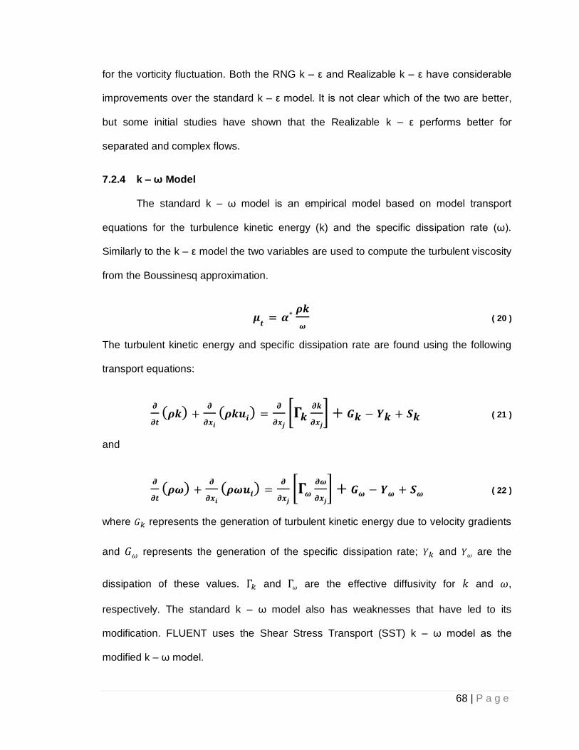
68 | P a g e
for the vorticity fluctuation. Both the RNG k – ε and Realizable k – ε have considerable
improvements over the standard k – ε model. It is not clear which of the two are better,
but some initial studies have shown that the Realizable k – ε performs better for
separated and complex flows.
7.2.4 k – ω Model
The standard k – ω model is an empirical model based on model transport
equations for the turbulence kinetic energy (k) and the specific dissipation rate (ω).
Similarly to the k – ε model the two variables are used to compute the turbulent viscosity
from the Boussinesq approximation.
( 20 )
The turbulent kinetic energy and specific dissipation rate are found using the following
transport equations:
( 21 )
and
( 22 )
where represents the generation of turbulent kinetic energy due to velocity gradients
and represents the generation of the specific dissipation rate; and are the
dissipation of these values. and are the effective diffusivity for and ,
respectively. The standard k – ω model also has weaknesses that have led to its
modification. FLUENT uses the Shear Stress Transport (SST) k – ω model as the
modified k – ω model.

69 | P a g e
The SST k – ω model improves on the standard k – ω model by creating a
gradual change from the standard version in the inner region of the boundary layer to a
high Reynolds number version of the k – ε model in the outer region of the boundary
layer. It also includes a modified turbulent viscosity formulation to account for shear
stress transport effects. These modifications make the SST k – ω model more accurate
and reliable for more flows, including adverse pressure gradients, airfoils, transonic
shock waves and more. Because of its ability to predict separation and adverse pressure
gradients, the SST k – ω model was chosen as the initial model and the other
turbulence models tested will be compared to it.
7.2.5 Transition k – kl – ω
From FLUENT’s theory guide(27): “The k – kl – ω transition model is used to
predict boundary layer development and calculate transition onset. This model can be
used to effectively address the transition of the boundary layer from a laminar to
turbulent regime.” For all of Roepke and Thomason’s testing the model had transition
strips located at 10% model length. After the flow was tripped, it remained turbulent the
rest of the body length, as verified by boundary layer stethoscope listening. Because of
this, for all CFD runs the flow was taken as turbulent over the whole body, as the first 4
inches of laminar flow was not seen as important as focusing on the separation on the
aft section. This led to the transition model not being need.
7.2.6 Transition Shear Stress Transport
The transition SST model is based on the SST k – ω model with the addition of
two more partial differential equations to estimate the location of transition between
laminar and turbulent flow, to make it a 4-equation model. Similarly to the k – kl – ω
transition model, the transition SST model was deemed un-necessary.

70 | P a g e
7.2.7 Reynolds Stress
The Reynolds stress model (RSM) is the most complicated model FLUENT
offers, as it is a 5-equation model. It no longer uses the Boussinesq approximation; it
assumes an anisotropic eddy-viscosity. The RSM better accounts for complex flows like
high streamline curvature, swirl, rotation, and rapid changes in strain rate than the zero,
one, and two equation models.
In the RSM the Reynolds stress is calculated through an expanded form that
relates the local time derivative and convection of the Reynolds stress to the turbulent
diffusion, molecular diffusion, stress production, buoyancy production, pressure strain,
dissipation, production by system rotation, and a user-defined source term. For more
details and implementation, the reader is directed to the FLUENT theory guide(27).
7.2.8 Wall Treatment
As said before the grid was created to give a y+ of less than 1 most places and
less than 2 everywhere. This allowed us to calculate the turbulence through the
boundary layer and we did not have to use any wall functions, the turbulence models are
valid through the near all region. If a y+ of less than 5 was not implemented then a y+
between 30 and 150 could be used in combination with wall functions. FLUENT’s theory
guide shows the difference between the two methods, as seen in Figure 52.

71 | P a g e
Figure 52: Visual comparison of near wall treatment methods(27)
These sizes are based on trying to get the cell nearest to the wall to fall in either
the viscous sublayer region, for the near-wall approach, or the fully turbulent log-law
region, for the wall functions. The different near-wall regions can be seen in Figure 53
below.
Figure 53: Zones in a typical incompressible turbulent boundary layer(26)

72 | P a g e
7.3 Operating Conditions
All meshing, computing, and post processing was done with ANSYS’s 12.1
software suite. The Mesh was generated in ICEM and then brought over to FLUENT.
Once in FLUENT the boundary conditions were set up, the flow as then initialized and
solve, and finally the post processing was also done in FLUENT.
7.3.1 Boundary Conditions
The boundary conditions were set up for the pressure based solver. The inlet, the
front face for the tunnel grids and the front/top side of the C-grids, were specified as
velocity inlets. The speed was matched to the wind tunnel data, with the inlet at 21.4 m/s
parallel to the axis and a speed of 2.25 m/s was used in the tunnel contraction geometry
to get the 21.4 m/s after the contraction. This was based on the 9.42:1 tunnel
contraction. The turbulence was also specified at the inlet, from the Flow Characteristics
in the Renovated 3x4ft Wind Tunnel paper(20), we used the turbulence intensity of 0.5%
and a mixing length of 0.08m. The mixing length was determined from mixing length =
0.07* hydraulic diameter, which is our tunnel diameter, giving us the value of 0.08m. The
outlet was modeled as an outflow condition, which in FLUENT, meant zero diffusion flux
for all flow variables and an overall mass balance correction. The fluxes were zero in the
plane normal to the exit boundary and they simulated a fully developed flow that had no
influence in the upstream direction. The bottom sections of the 2D geometry were
defined as the axis boundary. Here the rotation was assumed around the x-axis with the
origin at (0,0).
The body used no-slip wall conditions with the default values for wall roughness
height and other constants. There was no thermal, radiation, slip or any other

73 | P a g e
specifications enabled. The final boundary condition was for the fan in the aft section of
the body. In Cal Poly’s wind tunnel model there were pressure ports fore and aft of the
fan blades, which measured pressure rise across the fan disk. This was modeled as a
single plane in FLUENT and the pressure rise was modeled as a pressure jump across
that boundary. The pressure jump across the fan can be seen in Figure 54 below.
Figure 54: Contours of static pressure across the fan with a pressure increase of 500 pascals
7.3.2 Solver Conditions
FLUENT was run using a steady axisymmetric pressure-based solver with
absolute velocity formulation. The working fluid was FLUENT’s ‘air’ set as a constant
density of 1.225 kg/m3 and constant viscosity of 1.7894e-5 kg/m-s. The SIMPLE scheme
was used for pressure-velocity coupling. The gradient used the least squares cell based,
the pressure used second order, and the momentum, turbulent kinetic energy and
specific dissipation rate all used third order MUSCL schemes. To start off the under-

74 | P a g e
relaxation factors were brought down a little, then after the flow initialized, the under-
relaxation values were brought back to their default values.
7.3.3 Convergence Criteria
Three main convergence criteria were examined to test for convergence of the
model. First, the drag coefficient was checked to determine whether or not it has
stabilized. The flow was pretty well behaved and the drag coefficient would oscillate for a
few hundred iterations but then would dampen out pretty quickly to a single value. Next,
the mass flow rates at different stations throughout the slot were examined. When the
fan speed or other geometry was changed, these numbers no longer matched. This
meant that there was a mass imbalance within the slot and the solution needed more
iterations until a steady state was reached. The final item that was looked at was that the
changes have propagated far enough downstream that it no longer affected the body.
This was seen visually as what seemed like a wave propagated downstream as it
iterated. This was done because for small changes the flow around the body converged
faster than the wake did.
These three convergence criteria were examined looked for every case, but for
trials where multiple different settings were being tested, like fan speeds, a set number
of iterations were done for all settings to insure that all flows were converged to a
comparable degree. This was done for both simplicity and uniformity in case there was
something small that was sill changing but was not noticeable to any of the three
convergence criteria.

75 | P a g e
7.4 Computational Resources
The 2D axisymmetric cases were small enough to be run on available computers
overnight. The flight lab on campus was equipped with Dell Optiplex 755’s that had an
Intel Core 2 Quad CPU Q9450 with both processors clocked at 2.67GHz. They were
running Windows 7 64-bit with 4GB of RAM. These had enough space and power to run
the jobs overnight. Six computers were each set up with the ANSYS suite and each one
was able to run an independent job at the same time.

76 | P a g e
8 Results
We will first present the results from the CFD trials here, outlining the trends that are
found with the different operating conditions. Then in section 0 we will compare the CFD
results to Roepke and Thomason’s tunnel results.
8.1 Initial Testing and Observations
In the initial grid generation and solving, there were a number of initial test cases
that were used to both understand the software being run and the geometry that had to
be modeled. The ANSYS software suite had not been used previously and a lot of effort
in the beginning of the project was centered on learning the intricacies of the software.
Training began with using the tutorials for 2D meshing and solving in FLUENT, then
progressed to looking through the user manuals and theory guides to figure out what
settings could be modified and adjusted. Some confusion early in the process stemmed
from features being available for certain conditions but not for others. Eventually the grid
generation and solving process was understood and trustworthy answers were
achieved.
After the gridding and solving process was understood, more effort was put into
creating an improved geometry for the wind tunnel model. One of the initial problems
was the way ICEM discretized curves larger than a certain length. After a certain length
was reached, the curve fit created by ICEM was piecewise linear to the point where the
piecewise sections were larger than the grid used. As a result, the Cp values had an
unwanted visible wave for each section. The waviness was solved by using multiple
smaller independent curves to span the long forebody. The next modification was
performed after inspecting the wind tunnel model and noticing the lip on the aft section.
This was discussed earlier in section 5.1.3. Finally the different wind tunnel and the

77 | P a g e
freestream boundaries were modeled. The whole process was iterative and each time
something new was discovered, the geometry was modified and the flow solver was run
again.
8.2 CFD Run Matrix
The CFD test matrix, comprised of 10 cases, was not as comprehensive as was the
wind tunnel model test matrix which had 54 different runs. The goal was to see if the
CFD could accurately match the wind tunnel data and if the trends are in the same
direction. The plan was to start with a base configuration and vary one parameter to see
how it affected the results. We started with a base geometry that has cusp A and middle
slot gap of 0.385”. This was done for the free stream grid and then repeated for the
straight tunnel and the tunnel with the contraction. From these results we can tell the
difference the tunnel contraction has on the results and then move forward with the
condition that gives the best data that fits with Roepke and Thomason’s wind tunnel
results. After finding the best farfield geometry, that geometry was used for the rest of
the tests. The next runs were aimed at finding the minimum fan pressure needed for flow
attachment at the baseline configuration. Afterwards, results for four different turbulence
models were compared. Finally a grid independence study was done to verify that the
results were sufficiently independent of the domain discretization. This CFD test matrix
can be seen in Table 4 below.

78 | P a g e
Table 4: CFD test matrix
# Mesh Gap (in) Cusp Turbulence Model Fan Speed (ΔP [pa])
1 Freestream 0.385 A k-ω SST 0 and 500
2 Straight Tunnel 0.385 A k-ω SST “ ”
3 Contraction Tunnel 0.385 A k-ω SST “ ”
4 Straight Tunnel 0.385 A k-ω SST Found for attachment
5 “ ” 0.385 A Sparlart-Allmaras 0, 300, and 500
6 “ ” 0.385 A k-ε realizable “ ”
7 “ ” 0.385 A Reynolds Stress “ ”
8 Straight Coarse (67k) 0.385 A k-ω SST 0 and 500
9 Straight Mid (126k) 0.385 A k-ω SST “ ”
10 Straight Fine (230k) 0.385 A k-ω SST “ ”
All cases were run at standard sea level conditions with 21.2 m/s free stream
velocity. This was done because the 30 m/s data showed that the flow never was fully
attached to the aftbody for any of the fan speeds.
8.3 Goldschmied Body 20 m/s CFD Results
First we looked at the freestream condition solution to get an idea on how the body
behaves and digress into changing different parameters to see how the propulsor
behaves. This is done mainly by looking at the Cp distribution and fan speeds while
changing the tunnel shape and turbulence models to find their effects on the total drag
on the body.
8.3.1 Initial Freestream Solution
The first solution that ran was the freestream grid with the intermediate slot gap
of 0.385”, cusp A, k-ω SST turbulence model at both fan off and 500 pa pressure rise
across the fan. This fan pressure rise was high enough that the flow reattached to the aft
section, allowing us to compare the separated fan off case to the attached fan on case.

79 | P a g e
In the first image below, Figure 55, we can see filled contours for the two initial
cases with velocity magnitudes ranging from 0 to almost 30 m/s. The front of the body
had a low speed region leading up to the stagnation point at the nose. The flow then
accelerated over the top of the body. For the fan off case, the flow separated in front of
the slot entrance. For the fan on case, we see that the flow stayed attached, but still
dramatically slowed down over the aft body. The flow that was brought into the suction
slot sped up as it leaves the body. At the exit of the jet we see the highest velocity,
around 28.8 m/s, which is about 35% above freestream velocity.
Figure 55: Velocity contours (m/s) for fan off and fan on at 500 pascals
The next image, Figure 56, shows the pressure distribution for these flows. Both
flows have a high static pressure at the nose, due to the front stagnation point, then low
Fan ΔP=0 pa
Fan ΔP=500 pa

80 | P a g e
pressure at the thickest section as the flow accelerated around the body. For the fan off
case, there is little pressure recovery before the flow separated. In the separated region,
the pressure is relatively constant. This pressure differential, from front to rear, accounts
for a large portion of drag and was what the Goldschmied body aimed to reduce. For the
fan on case, we can see a large pressure jump in the internal sections. Also, there was a
lot higher pressure on the aft section, due to the re-attached flow. This is exactly what
Goldschmied was aiming for. There is one important item to note: as the fan is turned up
to higher speeds, low pressure region on the aft section of the body (seen in dark blue)
moves aft of the area of maximum thickness and closer to the slot entrance. This is very
important, as the low pressure on the aft section increased the pressure drag for that
section. This will be discussed in more detail later.
Figure 56: Pressure contours (pascals) for fan off and fan on at 500 pascals
Fan ΔP=0 pa
Fan ΔP=500 pa

81 | P a g e
The next image, Figure 57, looks at the streamlines going around the body. The
streamlines are colored by velocity to show fast and slow moving sections. For the fan
off case we saw that the circulation in the separated region went back through the slot in
the opposite direction. This allowed for the flow to come around the trailing edge, enter
the slot, and exit through the slot entrance. This is consistent with the experimental data,
as the slot was left open and allowed for the backflow. For the fan on case, the slot
sucked in the boundary layer streamlines and brought them through the slot. The faster
moving flow is then brought to the aft body and is slowed down from the diffuser effect of
the aft section.
Figure 57: Streamlines colored by velocity (m/s) for fan off and fan on at 500 pascals
Figure 58 is a close-up of the aft streamlines, giving more details on the aft
region and the flow through the internal slot.
Fan ΔP=500 pa
Fan ΔP=0 pa

82 | P a g e
Figure 58: Close up rear streamlines colored by velocity (m/s) for fan off and fan on at 500 pascals
From the figure above we see that there is a small separated region right after
the slot for the fan on case. A close up of this can be seen in Figure 59 below. As the
flow is brought into the suction slot there is a turning of the flow, and because of the flat,
blunt geometry, there is a stagnation point. The flow then has to turn past this flat section
and either enter the suction slot or move to the aft section. When moving aft, the flow
has to move over the small lip on the backside of the entrance. The lip caused the flow
that is moving over the aft section to form a small separation bubble. The flow then
reattached after this separation bubble. The reattachment can be seen in the previous
streamlines in Figure 58 above.
Fan ΔP=0 pa
Fan ΔP=500 pa

83 | P a g e
Figure 59: Inlet streamlines colored by velocity (m/s) for fan on at 500 pascals
Another interesting item was that the cusp was holding a trapped vortex, as was
described by Goldschmied and Ringleb. There was not enough time to test different
cusp or no cusp designs to find the importance of it, but it does seem to help bring the
flow around the corner and into the slot.
8.3.2 Tunnel Effects
The next item tested was the effects of the wind tunnel boundary walls on the
coefficient of pressure and the overall drag of the body. Figure 60 below shows the
velocity contours for the straight tunnel geometry. The slow moving boundary layer on
the tunnel walls can be seen in greenish/blue the top section of the figure. Besides this
change, the rest of the flow looked relatively similar to free stream conditions as covered
in the previous section.
Fan ΔP=500 pa

84 | P a g e
Figure 60: Velocity contours (m/s) for straight tunnel geometry
The velocity profile can also be seen for the tunnel geometry with the tunnel
contraction modeled in Figure 61 below. This geometry was examined to see if the
contraction led to uneven velocity distributions and radial flow components at the nose of
the model.
Figure 61: Velocity contours (m/s) for tunnel contraction geometry
The effect of these different tunnel geometries can be seen in the pressure
distributions on the body in Figure 62 and Figure 63. The Cp starts off at the stagnation
point, but does not drop as low through the area of maximum thickness as observed for
the wind tunnel models. At the lowest pressure, the freestream Cp is about 0.1 higher
than the two wind tunnel cases.

85 | P a g e
We see that the two tunnel geometries have nearly the same Cp curve for both
the power on and power off settings. This showed that the contraction has very little
effect on the pressure distribution.
Figure 62: Tunnel effects on body Cp for fan off conditions
Figure 63: Tunnel effects on body Cp for fan on at 500 pascals
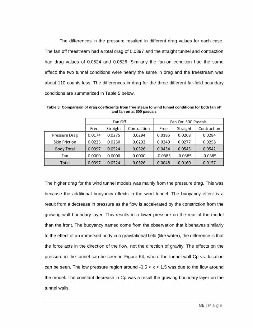
86 | P a g e
The differences in the pressure resulted in different drag values for each case.
The fan off freestream had a total drag of 0.0397 and the straight tunnel and contraction
had drag values of 0.0524 and 0.0526. Similarly the fan-on condition had the same
effect: the two tunnel conditions were nearly the same in drag and the freestream was
about 110 counts less. The differences in drag for the three different far-field boundary
conditions are summarized in Table 5 below.
Table 5: Comparison of drag coefficients from free steam to wind tunnel conditions for both fan off and fan on at 500 pascals
Fan Off Fan On: 500 Pascals
Free Straight Contraction Free Straight Contraction
Pressure Drag 0.0174 0.0275 0.0294 0.0185 0.0268 0.0284
Skin Friction 0.0223 0.0250 0.0232 0.0249 0.0277 0.0258
Body Total 0.0397 0.0524 0.0526 0.0434 0.0545 0.0542
Fan 0.0000 0.0000 0.0000 -0.0385 -0.0385 -0.0385
Total 0.0397 0.0524 0.0526 0.0048 0.0160 0.0157
The higher drag for the wind tunnel models was mainly from the pressure drag. This was
because the additional buoyancy effects in the wind tunnel. The buoyancy effect is a
result from a decrease in pressure as the flow is accelerated by the constriction from the
growing wall boundary layer. This results in a lower pressure on the rear of the model
than the front. The buoyancy named come from the observation that it behaves similarly
to the effect of an immersed body in a gravitational field (like water), the difference is that
the force acts in the direction of the flow, not the direction of gravity. The effects on the
pressure in the tunnel can be seen in Figure 64, where the tunnel wall Cp vs. location
can be seen. The low pressure region around -0.5 < x < 1.5 was due to the flow around
the model. The constant decrease in Cp was a result the growing boundary layer on the
tunnel walls.

87 | P a g e
Figure 64: Straight tunnel wall Cp
The two cases with wind tunnel walls also gave a higher skin friction drag then
the free air case. This was due to the fact that with the addition of the wall: the boundary
layer on the body was not able to expand as much, resulting in thinner boundary layer,
and the flow between the wall and the body was accelerated more than in freestream
conditions. These two factors led to higher local skin friction at the wall, which in turn led
to higher overall skin friction drag.
From the table we saw that the tunnel walls did have a large effect on the results
as compared to the free air case, but that the tunnel contraction was not much different
than the straight tunnel. Because of the differences between freestream and the tunnel,
with that of the collected wind tunnel data, the straight tunnel geometry will be used for
the remainder of this report.
8.3.3 Fan Effects
The next item looked at was the effect of the fan pressure rise on the aft body
attachment, pressure distribution, and drag for the body. The fan pressure increase was
varied from 0 to 1500 pascals in 100 Pa increments from 0 Pa to 600 Pa, and 1000 Pa
and 1500 Pa for the higher values.

88 | P a g e
Figure 65 shows the effects of the fan by plotting the Cp of the outer fore and aft
surfaces for the nine different fan settings. Looking at the aft section we saw that the
initial fan settings produce a large change in the pressure recovery, up to about 300 Pa.
After this point, it seemed that the flow was mostly re-attached and the increases in
pressure recovery after this point were small compared to the previous jumps. This
increase in pressure recovery was what Goldschmied was looking for, as high pressure
on the aft section gives the desired decrease in pressure drag of a body. Another
observation was that the suction flow created by the fan dramatically changes the fore
body pressure leading up to the slot, with the changes being seen as early as 50%
chord, 35% chord length in front of the slot. We saw that as the fan pressure rise was
increased, the Cp stayed low, around -0.45, for a longer time. This brings the adverse
pressure gradient further back, which delyaled the onset of separation, but also created
low pressure on the aft side of the maximum radius. This decrease in pressure on the aft
side of the maximum radius caused the pressure drag in that section to rise, which will
be discussed later.

89 | P a g e
Figure 65: Cp disribution for fan pressures of 0 to 1500 Pascals
One way to visually look at how the pressure changes effect the drag of the
vehicle is through a R2 vs. Cp plot. The R2 value is used because the body is
axisymmetric and that as you move out radially the area of each ‘station’ is proportional
to R2. The fore and aft sections of the body can be then plotted on the same plot. At a
single radius, if the front pressure is higher than the aft pressure there is a drag force
associated with that pressure differential. If it is the other way around, with a higher
pressure on the aft section, there is a thrusting force associated with it. The areas
associated with each region are related to the total body pressure force. R2 vs. Cp plots
can be seen for each of the nine fan attachment cases in Figure 66.

90 | P a g e
Figure 66: Cp vs. R2 values for varying fan pressures

91 | P a g e
From Figure 66 we see that an increase in fan speed does decrease the drag
and increase the thrust along the body aft of the suction slot (below approximately
R2~0.08). This increase comes at a huge cost in increased drag in front of the suction
slot. The pressure on the area aft of the maximum thickness, but in front of the suction
slot is decreased enough, that at higher fan pressures, it changes the once drag/thrust
region to a drag-dominated region that increases as fan pressure differential increases.
To better explore the effects of changes in fan pressure rise, each component of
drag was broken up and plotted independently. The first plot, Figure 67, shows the
break-up of the forces contributing to the drag seen on the CFD model. It breaks the
pressure forces up into the forebody (all the area in front of the slot), the aft body (all the
area behind the slot) and the slot (all of the internal slot areas) as seen in Figure 69. The
next force is the skin friction for the whole body. All of these are added together to get
the ‘Total Body Forces’. The first thing we see in the plot is that the axial force on the
forebody is increased significantly as fan pressure increases, which relates to a great
increase in drag. Next, the aftbody axial force is decreased as the fan pressure is
increased. The rest of the forces are relatively constant for the varying fan pressures.
When all the forces are added we see that the forebody and aftbody changes nearly
cancel each other out, creating a total body force that does not vary as much as the
single components. This leads to a nearly constant body drag force that actually slightly
increases as fan pressure differential increases beyond 350 Pa.

92 | P a g e
Figure 67: CFD Body axial force build-up for different fan speeds
Figure 68: Breakup of body sections between the fore, aft, and slot sectons
The total axial body force can then be added to the force that the fan exerts. The
fan force is found by taking the pressure differential across the fan and multiplying by the
fan area. Adding the fan and body forces we get the total force on the body, as would be
seen by a sting. The plot of this can be seen in Figure 69. As mentioned before, the

93 | P a g e
body forces are relatively constant and the fan really accounts for the reduction in axial
force, with a zero force estimated at a fan pressure around 750 pascals.
Figure 69: CFD Total force build-up for different fan speeds
Next, the inlet flow was looked at to see how the fan affected that area. Velocity
vector plots were taken at every pressure for the slot inlet and then plotted side by side
in Figure 70. With the fan off the flow separated pretty far upstream of the slot and there
is the recirculation region as expected for separated flows. An interesting feature is that
the flow has reversed through the slot, as part of the circulation region, and there is a
noticeable flow rate out of the inlet slot. At the 100 Pa fan pressure rise the flow has
switched back to the predicted direction, but the flow is not strong enough to change the
separated region much. Rather it changes the recirculation path and location. At 200 Pa
we see that the slot starts to ingest more flow, but it is still separated before and after the
slot. At this speed the streamlines are starting to bend to the aft section, but not enough

94 | P a g e
to reattach. At 300 Pa we see that the flow is brought down far enough to reattach to the
aft section, although it is still separated before the slot. The higher fan speeds continue
this pattern, bringing the flow closer to the aft section and reducing the forebody
separation. Full forebody attachment is obtained at 600 Pa. Another interesting feature
observed was that as the flow is turned into the suction slot, there is a part of the flow
that is brought radially into the aft body spacer. Running into this causes a stagnation
point and the flow to either side of this has to turn and go around each corner. This is not
ideal, and along with the rear lip, causes a separation bubble for a small region on the
aftbody. This is easier seen with the streamlines in Figure 59.
Figure 70: Velocity vector plots showing the flow at the inlet entrance for varying fan speeds
Fan Off 0 Pa
Fan On 100 Pa
Fan On 300 Pa
Fan On 200 Pa

95 | P a g e
Figure 70: Velocity vector plots showing the flow at the inlet entrance for varying fan speeds
Fan On 500 Pa
Fan On 400 Pa
Fan On 600 Pa
Fan On 1000 Pa
Fan On 1500 Pa

96 | P a g e
8.3.4 Turbulence Model Effects
Calculations were performed with four turbulence models were looked at to see
how this changed the solution. The models looked at were the Sparlart-Allmaras model,
the k-ε realizable model, the k-ω shear stress transport model, and the Reynolds stress
model. More details about each model can be seen in section 7.2, Turbulence Modeling,
on page 64.
Comparing the four models, the Sparlart-Allmaras model (a one equation model)
ended up being really far from the other three models, with drag values over double that
of the others. This difference can be seen in Figure 71 below.
Figure 71: Pressure drag coefficents for different turbulence models at different fan pressures
The differences between the k-ω SST and other turbulence models can be seen below
in Table 6 below.
0.000
0.020
0.040
0.060
0.080
0.100
0.120
0.140
0.160
0 100 200 300 400 500 600
Pre
ssu
re D
rag
Co
eff
icie
nt
Fan Pressure (pa)
S-A
k-ε realizable
k-ω SST
Reynolds SM

97 | P a g e
Table 6: Pressure Drag differences due to turbulence models for the straight tunnel at different fan pressures
Fan Pressure
k-ω SST (Cd,p)
S-A (% Diff)
k-ε realizable (% Diff)
Reynolds SM (% Diff)
0 0.050 138.8 -5.1 -3.1
300 0.051 153.3 13.4 9.2
500 0.054 155.1 11.6 3.2
The large difference between the Sparlart-Allmaras model and others was
concerning, as one would not expect that much difference. The Fluent Theory Guide (27)
states that; “The Spalart-Allmaras model was developed for aerodynamic flows. It is not
calibrated for general industrial flows, and does produce relatively larger errors for some
free shear flows, especially plane and round jet flows.” Our model has two areas that the
model is not calibrated for: it is more of a general industrial flow, as it is a large pipe and
not in freestream conditions. Secondly the exit jet from the fan has a large free shear
round jet flow. These un-calibrated flow regimes led to a lower pressure on the rear of
the model, resulting in significantly higher drag values.
The closeness of the k-ω SST model to other models, besides the S-A model, and
the previous knowledge that it performs well in separated flows led us to use it for the
turbulence model for all the other runs.

98 | P a g e
9 CFD Comparison to Cal Poly’s Tunnel Results
The first value looked at was the comparison of the pressure distributions over the
whole body compared to the wind tunnel to see how well CFD was able to predict the
flow. The first two plots, Figure 72 and Figure 73, were plotted independently for clarity
and then Figure 77 shows data for all power settings for the single cusp and slot width.
Even though these plots were at a single geometry, they were representative of the
whole data set, and changes from the cusp or slot width were not as pronounced as the
variations in pressure distribution caused by fan speed changes.
Figure 72: Comparison of Cp CFD data to Cal Poly experimental data for fan off conditions

99 | P a g e
Figure 73: Comparison of Cp CFD data to Cal Poly experimental data for the fan at 300 Pa
The first two plots show pretty good agreement between the CFD and the
experiential data, the main difference is the experimental cases had higher Cp values for
almost the entire length. This was interesting for the first half of the body because CFD
should have been able to predict the positive pressure gradient accurately over the nose
of the body.
The discrepancy may come from several factors; the first is that the static pressure
for the model was measured in the tunnel is not constant. This has an effect on the non-
dimensionalization process different depending on where exactly where the static
pressure is measured. From Figure 64 above we can see that the Cp can change by
about 0.25 per meter (roughly the length the test model).
The second form being the geometry is slightly different than then one being
modeled on the computer. The differences could arise because the actual wind tunnel

100 | P a g e
model was not measured; rather the original data points were used. The wind tunnel
model used the original data points to make the solid model, which in turn machined the
female mold. However, between the initial machining and the final product, there was
sanding, shaping, and possible differences in thickness which may have led to a slightly
different nose shape. Because a lack of time and resources we were not able to
compare the actual build model to the computer simulation. It was believed that the
geometry was not different enough to explain the differences.
Finally 3-D tunnel conditions were looked at to see if they had an effect on the
radial pressure distribution. This is important because the pressure ports for the
experimental data were on the right side of the model and there were no azimuthal ports
to see if the flow was truly axisymmetric. This involved looking at what effect the
rectangular tunnel cross section has and what effect model sideslip has.
A simple three dimensional computational model was made of the forebody
attached to a faired over aft section. This was then ran inviscidly to solely look at if the
pressure would vary and what kind of variation we might see. The first case was ran with
the model straight in the rectangular tunnel to see if the tunnel walls. It was found that
the rectangular cross section did not have an effect on the pressure distribution around
the body. This can be seen in the cross section of the results at 20% chord in Figure 74
below.

101 | P a g e
Figure 74: 3x4ft 3-D tunnel cross section static pressure contours for straight model at 20% chord
The computational model was then rotated to side slip angles of 2, 4, and 6
degrees to see how much that effected the pressure distribution. This had a large effect
as seen in previous experiments (see Figure 11 for Goldschmied’s rotation results). The
effect of two degrees of sideslip can be seen in the flow field and around the body in
Figure 75 below. This difference can be compared to the straight model to find how
much the pressure changes for each degree of sideslip, all referenced at 20% chord.
The correlation for small angles can be seen in Figure 76 below. Looking back to Figure
72 we see that there is about a 0.07 difference in Cp values between the experimental
and CFD results, when looking at the plot we see that this corresponds to about 1.9
degree sideslip angle. This small sideslip angle could explain the difference between the
CFD and the experimental result as there was no data to verify if the experimental model
was seeing radially constant conditions.

102 | P a g e
Figure 75: 3x4ft 3-D tunnel cross section static pressure contours with model in 2 degrees of beta at 20% chord
Figure 76: Correlation between Cp difference at 20% chord and side slip angle (beta)
y = -33.391x2 + 29.615x R² = 0.9999
0
1
2
3
4
5
6
7
0 0.05 0.1 0.15 0.2 0.25 0.3
Sid
e Sl
ip A
ngl
e (d
egre
es)
Cp differece at 20% chord

103 | P a g e
The pressure differences described above were present for all the fan settings,
which can be seen in Figure 77 and in detail in Figure 78. These plots also show a large
difference in the higher fan settings. The CFD took about 300 Pa fan difference for aft
body reattachment and at 1500 Pa the aft section had a maximum pressure recovery of
about 0.5. For the wind tunnel model, there was not aft body reattachment until about
1629 Pa and then at the maximum fan setting of 2349 Pa the maximum pressure
recovery was about 0.32. The CFD significantly over-predicted the pressure recovery on
the aft section and it did this at a much lower fan setting. When looking at these values
compared to Goldschmied’s and Peraudo et al. from Figure 19 on 24 above, the
maximum pressure recovery that they achieved was around 0.55, which is greater than
all the values that we have observed here. This led us to question that the wind tunnel
geometry or slot conditions were less than ideal, causing pressure recoveries that are
not as high as they could be. Also it is noted that the aft geometry, as outlined in section
5.1.3 on page 44, was modified from the SolidWorks model to make it a smoother shape
and may partially explain some of the difference. This also did not rule out the possibility
that the CFD model had a hard time predicting the separation point or pressure
recovery. Looking at possible reasons, the first may be that the separation point may
occur a little earlier on the tunnel model than on the CFD model. This would naturally
require more fan power to get the flow to re-attach and turn around the corner. Secondly,
if the lip on the aft section played a larger role than what CFD predicted we could expect
to see lower aft body pressure recoveries.

104 | P a g e
Figure 77: Comparison of Cp CFD data to Cal Poly experimental data for all fan conditions

105 | P a g e
Figure 78: Comparison of CFD fan speeds to Cal Poly experimental data: Aft Section
When comparing the total drag of the CFD model to the wind tunnel model, it was
difficult to get exact numbers because of the wide range of values measured from the
load cell on the sting. Figure 79 shows the measured axial force values for the fan
settings with different geometries. We assume that the drag values for the entire fan off
settings would be pretty similar, as the changes in geometry were all small and in the
separated region. The cusp and slot gap would be expected to have little effect in this
region, and no clear trend could be observed. The large variations of the fan off
conditions, going from the lowest drag coefficient of 0.043 to a maximum of 0.0714 and
a single outlier of 0.1263, appears to be an indication of the error involved with the data.

106 | P a g e
The CFD results of 0.056 fall close to the middle of this range, but it is hard to find an
error when there is not an exact value to compare to. From this data it seems that the
CFD was able to predict the drag of the fan off; it is within the data spread form the test.
For the rest of the data, additional trends were indistinguishable, as many of the
lines crossed over each other. Rather all we see is that the next axial force decreases as
fan speed increases. This shows that the fan is able to add a propulsive force, but slot or
cusp design have little influence. It seems that the differences that we are looking for
have a smaller effect than the overall error in the experiment.
Figure 79: Experimental axial force for different geometries at the 5 different fan settings
-0.0700
-0.0400
-0.0100
0.0200
0.0500
0.0800
0.1100
0.1400
0 100 200 300 400 500
Cd
Fan Power (Watts)
no cusp slot gap 0.154 no cusp slot gap 0.270 no cusp slot gap 0.385 no cusp slot gap 0.500 no cusp slot gap 0.615 cusp A slot gap 0.270 cusp A slot gap 0.385 cusp A slot gap 0.500 cusp A slot gap 0.615

107 | P a g e
10 Conclusion
When talking about the Goldschmied Propulsor to people, one of the main questions
asked by many people is; “Does the Propulsor actually work? And if so are the gains
enough to buy itself onto a vehicle?” From what Goldschmied originally claimed, up to a
50% reduction in drag from the most streamlined body, it seemed like it would have the
potential to buy itself onto a vehicle. Through our research we were not able to see
these gains. It actually turned out that the aft pressure recovery was counteracted by the
a reduction in pressure leading up to the slot, making almost no difference in pressure
drag when the fan was turned on. This shows that the smaller geometry tested in Cal
Poly’s wind tunnel was not able to replicate Goldschmied’s claims of reduced pressure
drag due to boundary layer ingestion.
On the other side, our research showed that the computational fluid dynamics
approach was able to replicate most of the wind tunnel data. The drag forces were within
the error bounds of the experimental data and the effect of the fan of the pressure
distribution showed the same trends. The CFD and wind tunnel started to differ in the
power needed for reattachment and the aft pressure recovery. In all cases, the CFD
analysis required a great deal less fan pressure rise to yield aft body reattachment. The
reason for this is not exactly known, rather it has been speculated that there are many
factors that have ledto this large difference. Some factors include earlier separation on
the main body, as earlier separation would take more effort to get to reattach. There
were more losses in the suction slot on the real model then what was able to be
modeled in an axisymmetric geometry. Also, a lot was learned from the different
conditions ran. There was a large effect on the pressure distribution on the model due to
the wind tunnel walls, but modeling the contraction or a rectangular cross section had
little difference between those and the straight circular model. Additionally, the two or

108 | P a g e
more equation turbulence models all produced similar results. From the grid
independence study for the structured axisymmetric conditions there was small error
(1.63%) using the GCI method.
Finally, it seemed that the tunnel effects had a large effect on the aft body, and
because of this the actual tunnel may accentuate what we saw going from freestream to
the wind tunnel cases. In conclusion, it seems that the tested geometry does not
produce the reduction in pressure drag we hoped for. There was potential for it to work,
but would require an optimized geometry to remove the low pressure region leading up
to the slot.
Figure 80: Flood filled velocity contours for max fan speed

109 | P a g e
11 Suggestions for Future Effort
From the computational study there were a few items noticed that might make the
test body perform better. It seemed that the shape was far from ideal and that a few
changes may make a large difference with the aft pressure distribution.
1) Modify the geometry to keep the natural fan off separation point closer in front of
the slot: This would reduce the suction need to keep the flow attached and
minimize the low pressure region on the back side of the maximum thickness
leading up to the slot and reduce the pressure drag that this low pressure region
creates.
2) Make the back side to the slot entrance sharper: Currently it seems that the flow
turns to enter the slot but the streamlines end up running into a flat section, which
greatly disrupts the flow. This leads to difficulty in aft body re-attachment.
3) Make the entrance to the slot smoother: Instead of trying to turn the flow 90° as it
enters the slot, something more gradual with the goal of decreasing the suction
needed to bring the flow to the fan.
4) Properly size motor and exit jet geometry: The current model uses an R/C motor
and fan meant to be used in a high speed airplane, but it saw relatively slow
moving air in the slot plenum. Because of this it is believed that the fan blades
are not the correct pitch and are at least partially stalled for most of their
operation. The exit geometry could be sized as either a diffuser or nozzle to get
the optimal exit pressure and velocity to give the greatest propulsive efficiency.

110 | P a g e
References
1. Goldschmied, Fabio. Wind Tunnel Test of the Modified Goldschmied Model with
Propulsion and Empennage: Analysis of Test Results. FRG-82-1 : David W. Taylor
Naval Ship R&D Center, 1982.
2. Goldschmied, Fabio R. On the Aerodynamic Optimization of Mini-RPV and Small GA
Aircraft. AIAA 1984-2163-960 : 2nd applied Aerodynamics Conference, Seattle, WA,
1984.
3. Roskam, Jan and Fillman, Greg. Design for minimum fuselage drag. 0021-8669
vol.13 no.8 (639-640) : Journal of Aircraft, 1976.
4. Boeing Commercial Airplanes. Current Market Outlook 2011-2030. Seattle, WA :
Boeing Market Anaylsis, 2011.
5. Bezos-O'Conner, Gaudy, et al. Fuel Efficiencies Through Airframe Improvements.
AIAA 2011-3530 : 3rd AIAA Atmospheric Space Environments Conference, 2011.
6. Nicholai, L. M. and Carichner, G. E. Fundamentals of Aircraft and Airship Design.
AIAA Educational Series : AIAA, Reston, VA, 2010.
7. Harshe, M., Pake, F. and Wasson, H. Investigation of A Boundary-Layer-Controlled
Airship. Akron, Ohio : Goodyear Aircraft Corporation, 1957.
8. Cerreta, P. A. Wind-Tunnel Investigation of the Drag of a Proposed Boundary-Layer
Controlled Airship. David W. Taylor Model Basin : Aero Rpt. 914, 1957.
9. Howe, Harvey. An Experimental Evaluation of a Low Propulsive Power, Discrete
Suction Concept applied to an Axisymmetric Vehicle. David Taylop Naval Ship
Research and Development Center : Bethesda, Maryland, 1982.
10. Goldschmied, Fabio. Fuselage Self-Propulsion by Static-Pressure Thrust: Wind-
Tunnel Verification. AIAA-87-2935 : AIAA/AHS/ASEE Aircraft Design, Systems and
Operations Meeting, 1987.
11. Betz, A. History of Boundary Layer Contol in Germany. "Boundary Layer and Flow
Control" by G.V. Lachmann : Pergamon Press, 1961.

111 | P a g e
12. Richards, E. J., Walker, W. S. and Greening, J. R. Tests of a Griffith Airfoil in the
13ft x 9ft Wind Tunnel. Ministry of Supply, London: His Majesty's Stationary Office :
Aeronautical Research Council Reports and Memoranda, 1944.
13. Goldschmied, Fabio R. Aerodynamic Hull Design for HASPA LTA Optimization.
AIAA-58418-412 : American Institute of Aerodynamics and Austronautics, 1978.
14. Ringleb, Friedrich. Seperation Control by Trapped Vortices. Boundary-Layer and
Flow Control, edited by G.V. Lachmann, Vol. I : Pergamon Press, New York, 1961.
15. Goldschmied, Fabio. Jet-Propulsion of Subsonic Bodies with Jet Total-Heal Equal
to Free Stream's. AIAA-83-1790 : AIAA Apploed Aerodynamics Conference, July 13-
15th, 1983.
16. Peraudo, P. N., Schetz, J. A. and Roy, C. J. Computational Study of the Embedded
Engine Static Pressure Thrust Propulsion System. Nashville, Tennessee : 50th AIAA
Aerospace Sciences Meeting including the New Horizons Forum and Aerospace
Exposition, January 2012.
17. Roepke, Joshua. An Investigation of a Goldschmied Propulsor. Masters Thesis :
California Polytechnic State University, San Luis Obispo, 2012.
18. Thomason, Nicole. Experimental Investigation of Suction Geometry on a
Goldschmied Propulsor. Masters Thesis : California Polytechnic State University,
San Luis Obispo, 2012.
19. Altmann, Greg. An Investigative Study of Gurney Flaps on a NACA 0036 Airfoil.
California Polytechnic State University Aerospace Engineering : Masters Thesis,
2011.
20. Thomas, Mathew L., Pandey, Dorian V. and Nguyen, Jason N. Flow
Characteristics of the Renovated Cal Poly 3 x 4 ft Subsonic Wind Tunnel. Senior
Project : California Polytechnic State University, San Luis Obispo, 2011.
21. Goldschmied, Fabio. Integrated Hull Design, Boundary-Layer Control, and
Propulsion of Submerged Bodies. AIAA-1699-658 : Second Propulsion Joint
Specialist Conference, Colorado Springs, CO, 1966.

112 | P a g e
22. Crowe, Clayton, et al. Engineering Fluid Mechanics. R.R. Donnelley/Jefferson City :
John Wiley & Sons, INC, 2009.
23. White, Frank. Viscous Fluid Flow. New York, NY : McGraw-Hill, 2006.
24. Celik, Ismail, et al. Procedure for Estimation and Reporting of Uncertainty Due to
Discritization in CFD Applications. Journal of Fluid Mechanics : Volume 130, July,
2008.
25. Oberkampf, William and Roy, Christopher. Verification adn Validation in Scientific
Computing. Cambridge, New York : Cambridge University Press, 2010.
26. Tannehill, John, Anderson, Dale and Pletcher, Richard. Computational Fluid
Mechanics and Heat Transfer. Philadelphia, PA : Taylor & Francis, 1997.
27. ANSYS. ANSYS FLUENT Theory Guide. Release 13.0 : s.n., November, 2010.
28. ANSYSS. ANSYS FLUENT User's Guide. Release 13.0 : s.n., November 2010.
29. Wilcox, David. Turbulence Modeling for CFD. San Diego, CA : Birmingham Press,
2004.

113 | P a g e
Appendix A: Model Geometry Points
Forebody Geometry Points:
X Y Z
0.0000E+00 -1.2382E-07 0.0000E+00
1.0000E-02 1.8893E-02 0.0000E+00
2.0000E-02 3.0980E-02 0.0000E+00
3.0000E-02 3.9956E-02 0.0000E+00
4.0000E-02 4.7498E-02 0.0000E+00
5.0000E-02 5.4294E-02 0.0000E+00
6.0000E-02 6.0594E-02 0.0000E+00
7.0000E-02 6.6483E-02 0.0000E+00
8.0000E-02 7.1999E-02 0.0000E+00
9.0000E-02 7.7177E-02 0.0000E+00
1.0000E-01 8.2056E-02 0.0000E+00
1.1000E-01 8.6676E-02 0.0000E+00
1.2000E-01 9.1072E-02 0.0000E+00
1.3000E-01 9.5271E-02 0.0000E+00
1.4000E-01 9.9292E-02 0.0000E+00
1.5000E-01 1.0315E-01 0.0000E+00
1.6000E-01 1.0684E-01 0.0000E+00
1.7000E-01 1.1039E-01 0.0000E+00
1.8000E-01 1.1379E-01 0.0000E+00
1.9000E-01 1.1705E-01 0.0000E+00
2.0000E-01 1.2018E-01 0.0000E+00
2.1000E-01 1.2318E-01 0.0000E+00
2.2000E-01 1.2607E-01 0.0000E+00
2.3000E-01 1.2884E-01 0.0000E+00
2.4000E-01 1.3152E-01 0.0000E+00
2.5000E-01 1.3408E-01 0.0000E+00
2.6000E-01 1.3655E-01 0.0000E+00
2.7000E-01 1.3893E-01 0.0000E+00
2.8000E-01 1.4120E-01 0.0000E+00
2.9000E-01 1.4338E-01 0.0000E+00
3.0000E-01 1.4547E-01 0.0000E+00
3.1000E-01 1.4746E-01 0.0000E+00
3.2000E-01 1.4936E-01 0.0000E+00
3.3000E-01 1.5117E-01 0.0000E+00
3.4000E-01 1.5290E-01 0.0000E+00
3.5000E-01 1.5454E-01 0.0000E+00
3.6000E-01 1.5609E-01 0.0000E+00
3.7000E-01 1.5757E-01 0.0000E+00
3.8000E-01 1.5896E-01 0.0000E+00
3.9000E-01 1.6027E-01 0.0000E+00
4.0000E-01 1.6150E-01 0.0000E+00
4.1000E-01 1.6265E-01 0.0000E+00
4.2000E-01 1.6372E-01 0.0000E+00
4.3000E-01 1.6471E-01 0.0000E+00
4.4000E-01 1.6562E-01 0.0000E+00
4.5000E-01 1.6645E-01 0.0000E+00
4.6000E-01 1.6719E-01 0.0000E+00
4.7000E-01 1.6786E-01 0.0000E+00
4.8000E-01 1.6843E-01 0.0000E+00

114 | P a g e
4.9000E-01 1.6893E-01 0.0000E+00
5.0000E-01 1.6933E-01 0.0000E+00
5.1000E-01 1.6965E-01 0.0000E+00
5.2000E-01 1.6987E-01 0.0000E+00
5.3000E-01 1.7000E-01 0.0000E+00
5.4000E-01 1.7003E-01 0.0000E+00
5.5000E-01 1.6995E-01 0.0000E+00
5.6000E-01 1.6977E-01 0.0000E+00
5.7000E-01 1.6949E-01 0.0000E+00
5.8000E-01 1.6909E-01 0.0000E+00
5.9000E-01 1.6859E-01 0.0000E+00
6.0000E-01 1.6798E-01 0.0000E+00
6.1000E-01 1.6727E-01 0.0000E+00
6.2000E-01 1.6644E-01 0.0000E+00
6.3000E-01 1.6551E-01 0.0000E+00
6.4000E-01 1.6446E-01 0.0000E+00
6.5000E-01 1.6329E-01 0.0000E+00
6.6000E-01 1.6201E-01 0.0000E+00
6.7000E-01 1.6059E-01 0.0000E+00
6.8000E-01 1.5903E-01 0.0000E+00
6.9000E-01 1.5732E-01 0.0000E+00
7.0000E-01 1.5546E-01 0.0000E+00
7.1000E-01 1.5344E-01 0.0000E+00
7.2000E-01 1.5124E-01 0.0000E+00
7.3000E-01 1.4886E-01 0.0000E+00
7.4000E-01 1.4628E-01 0.0000E+00
7.5000E-01 1.4346E-01 0.0000E+00
7.6000E-01 1.4038E-01 0.0000E+00
7.7000E-01 1.3698E-01 0.0000E+00
7.8000E-01 1.3318E-01 0.0000E+00
7.9000E-01 1.2891E-01 0.0000E+00
8.0000E-01 1.2404E-01 0.0000E+00
8.1000E-01 1.1840E-01 0.0000E+00
8.2000E-01 1.1168E-01 0.0000E+00
8.3000E-01 1.0327E-01 0.0000E+00
Cusp and Front Geometry Points:
X Y Z
8.3626E-01 9.6637E-02 0.0000E+00
8.3772E-01 9.4934E-02 0.0000E+00
8.3851E-01 9.3633E-02 0.0000E+00
8.3933E-01 9.1948E-02 0.0000E+00
8.3882E-01 9.1069E-02 0.0000E+00
8.3846E-01 9.0014E-02 0.0000E+00
8.3825E-01 8.9186E-02 0.0000E+00
8.3808E-01 8.7860E-02 0.0000E+00
8.3805E-01 8.6425E-02 0.0000E+00
8.3806E-01 8.5058E-02 0.0000E+00
8.3476E-01 8.5090E-02 0.0000E+00
8.2996E-01 8.5090E-02 0.0000E+00
8.0380E-01 2.4638E-02 0.0000E+00
8.0380E-01 0.0000E+00 0.0000E+00

115 | P a g e
Aftbody and Fan Points:
X Y Z
8.5719E-01 0.0000E+00 0.0000E+00
8.6319E-01 1.0000E-02 0.0000E+00
8.7319E-01 1.5000E-02 0.0000E+00
8.7319E-01 3.4500E-02 0.0000E+00
8.6219E-01 3.4500E-02 0.0000E+00
8.5825E-01 3.5019E-02 0.0000E+00
8.5457E-01 3.6542E-02 0.0000E+00
8.5141E-01 3.8964E-02 0.0000E+00
8.4899E-01 4.2120E-02 0.0000E+00
8.4747E-01 4.5796E-02 0.0000E+00
8.4695E-01 4.9740E-02 0.0000E+00
8.4695E-01 8.5560E-02 0.0000E+00
8.4704E-01 8.6217E-02 0.0000E+00
8.4729E-01 8.6830E-02 0.0000E+00
8.4769E-01 8.7356E-02 0.0000E+00
8.4822E-01 8.7760E-02 0.0000E+00
8.4883E-01 8.8013E-02 0.0000E+00
8.4949E-01 8.8100E-02 0.0000E+00
8.5269E-01 8.8100E-02 0.0000E+00
8.6299E-01 7.6800E-02 0.0000E+00
8.7709E-01 6.3800E-02 0.0000E+00
8.8589E-01 5.7500E-02 0.0000E+00
8.9469E-01 5.2200E-02 0.0000E+00
9.0349E-01 4.6900E-02 0.0000E+00
9.2109E-01 3.8800E-02 0.0000E+00
9.4759E-01 2.9700E-02 0.0000E+00
9.8279E-01 2.3800E-02 0.0000E+00
9.4869E-01 2.7000E-02 0.0000E+00
9.1869E-01 3.4500E-02 0.0000E+00
8.8869E-01 3.4500E-02 0.0000E+00
8.8869E-01 1.5000E-02 0.0000E+00
9.1869E-01 1.5000E-02 0.0000E+00
9.4869E-01 1.5000E-02 0.0000E+00
9.4869E-01 0.0000E+00 0.0000E+00