analysis and numerical solutions of delay differential ... · analysis and numerical solutions of...
TRANSCRIPT

Analysis and Numerical solutions ofDelay Differential-Algebraic Equations
vorgelegt von
Phi Ha
geb. in NamDinh, Vietnam
von der Fakultät II - Mathematik und Naturwissenschaften
der Technischen Universität Berlin
zur Erlangung des akademischen Grades
Doktor der Naturwissenschaften
- Dr. rer. nat. -
genehmigte Dissertation
Promotionsausschuss:
Vorsitzender: Prof. Dr. Yuri Suris
Gutachter: Prof. Dr. Volker Mehrmann
Gutachter: Prof. Dr. Peter Kunkel
Gutachterin: Prof. Dr. Caren Tischendorf
Tag der wissenschaftlichen Aussprache: 09. März 2015
Berlin 2015


Acknowledgments
Doing a PhD is a long hard work, and during the time working on this thesis, I have
received the support from many persons.
First and foremost, I would like to express my deep gratitude to my advisor Prof.
Dr. Volker Mehrmann for introducing me to the topic of Delay-DAEs, for his patience,
support, advice and criticism. My thanks also go to all my colleagues in the Numerical
group of the Technical University Berlin, where I have enjoyed the friendly atmosphere
and the productive work environment. In addition, personal thanks are due to my
former office mate Tobias Brüll, for being my weird and special friend, and also for his
emotional suggestion to the behavior approach; to Helia Niroomandrad for three years
sharing office with me; to Andreas Steinbrecher for many good and free lessons about
DAEs; to Benjamin Unger for carefully reading this work and many valuable correc-
tions and suggestions. Assistance provided by Ma Vinh Tho was greatly appreciated.
I also wish to acknowledge the help and support in living and working provided by
my Vietnamese friends, in particular Dr. Dam Quoc Phoi. With your friendship, you
really lighted up my last one and half year in Berlin.
I’m grateful that this work is supported by the DFG project SFB 910 Control of self-
organizing nonlinear systems: Theoretical methods and concepts of application during
my four year PhD at the Technical University Berlin. As a student, I also want to thank
the Berlin Mathematical School for their support, in particular the transition period
during the end of Phase I and the beginning of Phase II.
Finally, this thesis is dedicated to my parents and my brother. Without my family’s
encouragement, love and support, this work would never have been existent.


Zusammenfassung
In dieser Arbeit legen wir die Grundlage für die Analyse der Lösbarkeit von Anfangs-wertproblemen (IVPs) für verzögerte differentiell-algebraische Gleichungen (DDAEs).Eine DDAE ist eine allgemeine Kombination von zwei mathematischen Objekten: dif-ferentiell-algebraischen Gleichungen (DAEs) und Differentialgleichungen mit Zeitver-zögerungen (DDEs). Diese Kombination führt zu vielen Schwierigkeiten in der Analysevon DDAEs, die weder für DAEs noch für DDEs auftreten. Zwei von diesen Schwie-rigkeiten, die große Auswirkungen auf die theoretische und numerischen Lösung vonDDAEs haben, sind die Nicht-Kausalität und das Vorlaufen (advancedness) eines Sys-tems, die bisher für DDAEs nicht diskutiert wurden. Diese Schwierigkeiten zu überwin-den und neue Erkenntnisse über die Analyse der Lösbarkeit von DDAEs zu entwickelnsind das Thema der Arbeit, deren Inhalt aus drei wesentlichen Schwerpunkten besteht.
Das Studium von linearen DDAE Systemen mit variablen Koeffizienten ist der ersteSchwerpunkt der Arbeit. Im Gegensatz zu kausalen DDAEs, die sich ähnlich wie DAEsverhalten, muss (sogar für lineare) nichtkausale DAEs die Strukturtheorie von mehr alszwei Matrizen verwendet werden, und daher kann die Analyse der Lösbarkeit der ent-sprechenden IVPs durch die klassische Theorie von Matrizenpaaren nicht angewen-det werden. Ein wichtiger Beitrag des ersten Teils der Arbeit ist, den Zusammenhangzwischen Existenz und Eindeutigkeit von Lösungen von IVPs für DDAEs und der Regu-larität von entweder einem Matrizenpaar oder einem Matrizentripel zu untersuchen.Hierbei ist zu unterscheiden, ob das Zeitintervall beschränkt oder unbeschränkt ist.Das erzielte Ergebnis erlaubt uns, die Lösbarkeit einer linearen DDAE durch Spektra-leigenschaften der Koeffizientenmatrizen zu studieren. Wir wenden Matrix-Polynomean, um die Lösbarkeit einer großen Klasse von zeitverzögerten Systemen einschließ-lich unter- und überbestimmter Systeme zu analysieren. Zwei Klassen von DDAEs, diehäufig in Anwendungen Verwendung finden sind DDAEs vom retardierten und vomneutralen Typ. Für diese beiden wichtigen Klassen untersuchen wir einen weiteren,insbesondere algebraischen Ansatz zur Analyse ihrer Lösbarkeit. Dieser Ansatz zeigtdie Ähnlichkeit dieser zwei Typen von DDAEs zu DAEs, und ist geeignet für weitereStudien über Eigenschaften hinsichtlich Regelung und Steuerung von DDAEs.
Um die theoretische Grundlage für die numerische Lösung von IVPs für DDAEszu erzielen, betrachten wir als zweiten Schwerpunkt allgemeine Systeme mit linea-ren zeitvarianten Koeffizienten. Es wird gezeigt, dass klassische schrittweise Metho-de (’Method of steps’) für nichtkausale Systeme nicht anwendbar ist, und es werdenzwei neue Ansätze für die Regularisierung von allgemeinen linearen DDAEs vorgestellt.Der erste Ansatz modifiziert die ’method of steps’ so, dass die Lösung auf fortschrei-tenden Teilintervallen des Integrationsbereichs berechnet werden kann. Es wird ein

Shift-Index eingeführt, der ein Maß für die Nichtkausalität des System darstellt. Damitwird die Regularisierungstheorie von DAEs auf DDAEs verallgemeinert. Abhängig vomTyp von der DDAE, führt diese Regularisierungstechnik zu verschiedenen strangeness-freien Formulierungen, die sehr kompliziert sein können, falls eine DDAE von vorlau-fendem Typ ist. Die zweite Methode formuliert das AWP für die DDAE als ein Rand-wertproblem (RWP) für eine hochdimensionale DAE um, sodass die DAE Theorie fürdie Regularisierung angewendet werden kann. Weiter wird gezeigt, dass die so konstru-ierte DAE in diesem differentiell-algebraischen RWP einen beliebig großen Strangen-essindex haben kann.
Der letzte Teil der Arbeit ist die Entwicklung von zwei neuen Integrationsalgorith-men für allgemeine lineare DDAEs, welche auf den Ansätzen des zweiten Teils dieserArbeit basieren. Die Hauptidee dieser Algorithmen ist es, bekannte numerische Me-thoden (für DDEs und für DAEs) auf die strangeness-freie Formulierung anzuwenden,die über oben genannte Regularisationstechniken erhalten wird. Der erste Algorith-mus, der auf einer Verallgemeinerung der ’Method of Steps’ basiert, behandelt DDAEsvon retardierten und neutralen, aber nicht von vorlaufendem Typ. Der zweite Algo-rithmus, welcher differentiell-algebraische RWPe löst, ist für alle drei Typen geeignet.Abschließend zeigen wir die Effizienz und Robustheit der vorgestellten Algorithmenim Vergleich mit dem häufig benutzten numerischen Softwarepaket RADAR5 [60].

Abstract
With this thesis, we aim to lay the foundation for the solvability analysis of initial valueproblems (IVPs) for delay differential-algebraic equations (DDAEs). In our context, aDDAE is a general combination of two important mathematical objects: differential-algebraic equations (DAEs) and delay differential equations (DDEs). This combinationhas led to many difficulties in the analysis of DDAEs, which occur neither for DAEs norfor DDEs. Two of these difficulties, which have strong influence on the theoretical andnumerical solutions of DDAEs, are the noncausality and the advancedness of a system,previously not discussed for DDAEs. To overcome these difficulties in order to give newinsights to the solvability analysis of DDAEs is the purpose of this work, whose maincontent is focused on three topics presented in the following.
The investigation of systems with time invariant coefficients is the first topic of in-terest. In contrast to causal DDAEs, which possess many similar properties like DAEs,already in the linear case, noncausal DDAEs take into account the structure of morethan two matrices and consequently, the solvability analysis of the corresponding IVPscan not be completely analyzed by the classical theory of matrix pairs. An importantcontribution of the first part of this thesis is to point out the link between the existenceand uniqueness of solutions of IVPs for DDAEs and the regularity of either a matrix pairor a matrix triple, depending on whether the time interval is bounded or not. This re-sult allows to study the solvability of a linear DDAE by investigating spectral propertiesof its matrix coefficients. In more details, we apply a matrix polynomial approach tostudy the solvability analysis for a much broader class of time delay systems includingboth under- and overdetermined systems. Another approach in the theory of DAEs,namely an algebraic method, is examined to study general DDAEs of retarded and neu-tral types, which usually occur in applications. This approach has shown the similaritybetween these two types of DDAEs and DAEs, and it is suitable for further investigationon control properties of DDAEs.
Aiming at the theoretical background for the solution procedure for DDAEs, thesecond topic involves the consideration of general systems with linear time varyingcoefficients. Observing the failure of the classical method of steps for noncausal sys-tems, we propose two new approaches for the regularization of general linear DDAEs.The first approach aims to modify the method of steps so that one can compute thesolution on consecutive sub-intervals of the integration time interval. By introduc-ing the shift index concept to estimate the noncausality of a system, we generalize theregularization procedure of DAEs for DDAEs. Depending on the types of DDAEs, thisregularization technique leads to different strangeness-free formulations, which canbe very complicated if a DDAE is of advanced type. On the other hand, the second ap-

proach reformulates an IVP for a DDAE as a BVP for a high dimensional DAE so that onecan make use of the DAE theory for the regularization. It is further shown that the con-structed DAE in this differential-algebraic BVP can have an arbitrarily high strangenessindex.
The last part of this thesis is the development of two new integration algorithmsfor general linear DDAEs by using the two approaches introduced in the second part.The main core of these algorithms is to apply well-known numerical methods (forDDEs or for DAEs) to the strangeness-free formulation obtained by different regular-ization techniques discussed above. The first algorithm, based on a generalization ofthe method of steps, successfully handles DDAEs of retarded and neutral types but notsystems of advanced type. On the other hand, the second algorithm, based on solvingdifferential-algebraic BVPs, is suitable for dealing with all three types of DDAEs. Con-cluding, the efficiency and robustness of both algorithms are demonstrated in com-parison with the commonly used numerical solver RADAR5 [60].

Eidesstattliche Versicherung
Hiermit versichere ich an Eides statt, dass ich die vorliegende Arbeit selbstständig und
ohne Benutzung anderer als der angegebenen Hilfsmittel angefertigt habe. Die aus
fremden Quellen direkt oder indirekt übernommenen Gedanken sind als solche kennt-
lich gemacht.
Teile der vorliegenden Arbeit sind in Kooperation mit Prof. Dr. Volker Mehrmann und
Dr. Andreas Steinbrecher entstanden und sind als solche kenntlich gemacht. Kapitel 2,
3 und 5 zitieren Ergebnisse der Artikel
[63] Analysis and Reformulation of Linear Delay Differential-Algebraic Equations.
P. Ha and V. Mehrmann. Electr. J. Lin. Alg., Vol. 23 (2013), pp. 703-730, 2013,
[65] Analysis of Linear Variable Coefficient Delay Differential-Algebraic Equations.
P. Ha, V. Mehrmann and A. Steinbrecher. J. Dynam. Differential Equations, pp.
1-26, 2014.
Die, in den Artikeln [63, 65], diskutieren Ideen und deren Umsetzung sowie die Lite-
raturrecherche waren überwiegend bis außschließlich mein Anteil. Die Ausarbeitung
dieser Artikel wurde mehrheitlich von mir ausgeführt. Prof. Dr. Volker Mehrmann und
Dr. Andreas Steinbrecher standen mir dabei mit ihrem Wissen und ihrer Erfahrung zur
Seite.
Berlin, den 04. Dezember 2014


Erklärung
Hiermit erkläre ich, die vorliegende Arbeit weder im Inland noch im Ausland in glei-
cher oder ähnlicher Form als Dissertation, Diplom- oder ähnliche Prüfungsarbeit an-
gemeldet oder eingereicht zu haben und weiterhin keine Promotionsabsicht an einer
anderen Hochschule oder Fakultät beantragt zu haben.
Der wissenschaftliche Inhalt der Arbeit wurde weder in seiner Vollständigkeit noch in
der vorliegenden Form veröffentlicht.
Kapitel 5 ist jeweils die überarbeitete und erweiterte Fassungen des Preprints
[64] Analysis and numerical solution of linear delay differential-algebraic equations.
P. Ha and V. Mehrmann, in preparation.
Kapitel 2, 3 und 5 zitieren Ergebnisse der Artikel
[63] Analysis and Reformulation of Linear Delay Differential-Algebraic Equations.
P. Ha and V. Mehrmann. Electr. J. Lin. Alg., Vol. 23 (2013), pp. 703-730, 2013,
[65] Analysis of Linear Variable Coefficient Delay Differential-Algebraic Equations.
P. Ha and V. Mehrmann and A. Steinbrecher. J. Dynam. Differential Equations,
pp. 1-26, 2014.
Berlin, den 04. Dezember 2014


Contents
Nomenclature xix
Abbreviation xxi
1 Introduction 1
1.1 Applications . . . . . . . . . . . . . . . . . . . . . . . . . . . . . . . . . . . . . 4
1.1.1 Human balance control and multibody control systems . . . . . . . 4
1.1.2 Time-delayed electric circuits . . . . . . . . . . . . . . . . . . . . . . . 7
1.1.3 DDAEs in fluid dynamics . . . . . . . . . . . . . . . . . . . . . . . . . 8
1.1.4 DDAEs in chemical engineering . . . . . . . . . . . . . . . . . . . . . 9
2 Fundamentals of DAEs and DDEs 11
2.1 Time Invariant Differential-Algebraic Equations . . . . . . . . . . . . . . . . 11
2.2 Time Varying Differential-Algebraic Equations . . . . . . . . . . . . . . . . . 13
2.3 High-order Differential-Algebraic Equations . . . . . . . . . . . . . . . . . . 21
2.4 Classification of DDEs . . . . . . . . . . . . . . . . . . . . . . . . . . . . . . . 24
2.5 Solution concepts and the method of steps for DDEs . . . . . . . . . . . . . 25
3 Fundamentals of DDAEs 29
3.1 Basic concepts of DDAEs . . . . . . . . . . . . . . . . . . . . . . . . . . . . . 29
3.2 Prior work on DDAEs . . . . . . . . . . . . . . . . . . . . . . . . . . . . . . . . 32
3.3 Characteristics of general linear DDAEs . . . . . . . . . . . . . . . . . . . . . 35
3.4 Transforming multiple delays into single delay . . . . . . . . . . . . . . . . . 38
4 Solvability Analysis of General Linear Time Invariant DDAEs 41
4.1 Basic properties . . . . . . . . . . . . . . . . . . . . . . . . . . . . . . . . . . . 41
xiii

Contents xiv
4.2 Systems on bounded time intervals . . . . . . . . . . . . . . . . . . . . . . . 43
4.3 Systems on unbounded time intervals . . . . . . . . . . . . . . . . . . . . . . 47
4.3.1 Structures of matrix triples via constant equivalence transforma-
tions . . . . . . . . . . . . . . . . . . . . . . . . . . . . . . . . . . . . . 47
4.3.2 A matrix polynomial approach . . . . . . . . . . . . . . . . . . . . . . 54
4.3.3 Reformulation of non-advanced systems . . . . . . . . . . . . . . . . 59
5 Solvability Analysis of General Linear Time Varying DDAEs 63
5.1 Generalization of the method of steps . . . . . . . . . . . . . . . . . . . . . . 64
5.2 Solvability analysis via system classification . . . . . . . . . . . . . . . . . . 70
5.3 Regularization of DDAEs by operational arrays . . . . . . . . . . . . . . . . 73
5.4 Boundary Value Problem method . . . . . . . . . . . . . . . . . . . . . . . . 79
6 Numerical solutions of IVPs for DDAEs 87
6.1 Application of the generalized method of steps for DDAEs . . . . . . . . . . 87
6.2 Application of the BVP method to DDAEs . . . . . . . . . . . . . . . . . . . . 89
6.3 Examples . . . . . . . . . . . . . . . . . . . . . . . . . . . . . . . . . . . . . . . 93
7 Solvability Analysis of General Nonlinear DDAEs 97
Conclusion and Outlook 101
Conclusion . . . . . . . . . . . . . . . . . . . . . . . . . . . . . . . . . . . . . . . . . 101
Outlook . . . . . . . . . . . . . . . . . . . . . . . . . . . . . . . . . . . . . . . . . . . 103

List of Figures
1.1 Inverted one-bar pendulum . . . . . . . . . . . . . . . . . . . . . . . . . . . . 5
1.2 Time-delayed electric circuit, [97], p. 536. . . . . . . . . . . . . . . . . . . . . 7
1.3 Williams-Otto process, [109], p. 304. . . . . . . . . . . . . . . . . . . . . . . . 9
2.1 Classification of DDEs with discrete delays, compare [120]. . . . . . . . . . 25
2.2 Discontinuity propagation of the solutions to (2.25) (left) and (2.26) (right). 26
3.1 Numerical solution and absolute error of the IVP (1.2) for (3.19) with con-
stant stepsize h = 0.1. . . . . . . . . . . . . . . . . . . . . . . . . . . . . . . . . 35
5.1 Absolute error vs. length of the time interval I for (5.45). . . . . . . . . . . . 84
5.2 Numerical solution and absolute error of (5.46). . . . . . . . . . . . . . . . . 85
6.1 Numerical solution and absolute error of the IVP (6.7) with constant step-
size h = 0.01. . . . . . . . . . . . . . . . . . . . . . . . . . . . . . . . . . . . . . 90
6.2 Numerical solution and absolute error of the IVP (6.14) with constant
stepsize h = 0.01. . . . . . . . . . . . . . . . . . . . . . . . . . . . . . . . . . . 93
6.3 Relative error of the DDAE (6.15) (left) and of the DDAE (6.16) (right) with
constant stepsize h = 0.01. . . . . . . . . . . . . . . . . . . . . . . . . . . . . . 95
6.4 The solution and the absolute error of the DDAE (6.17) with constant
stepsize h = 0.01. . . . . . . . . . . . . . . . . . . . . . . . . . . . . . . . . . . 96
xv

List of Figures xvi

List of Tables
5.1 Strangeness-free formulation for different classes of DDAEs. . . . . . . . . 73
5.2 Consistency of initial conditions for different classes of DDAEs. . . . . . . 74
5.3 Theoretical comparison of the generalized method of steps and the BVP
method. . . . . . . . . . . . . . . . . . . . . . . . . . . . . . . . . . . . . . . . 85
xvii

List of Tables xviii

Nomenclature
m number of equations
n number of unknowns
I= [0, t f ) time interval
Iτ = [−τ, t f ) time interval including history
N0 (resp.,N) set of non-negative (resp., positive) integer numbers
Z (resp.,Q) set of integer numbers (resp., rational numbers)
R (resp., R+) set of real numbers (resp., positive real numbers)
C set of complex numbers
Rm,n (resp., Cm,n) set of m by n matrices whose entries are in R (resp., C)
Cm,n[ξ] set of m by n matrix polynomials of variable ξ, p. 55
C k (I,Cn) vector space of all k-times continuously differentiable functions
from I into Cn
x, x, x(i ) total derivatives of x(t ) with respect to t
σ(E , A) spectrum of a matrix pair (E , A), p. 9
σ(E , A,B) spectrum of a matrix triple (E , A,B), p. 33
ν (or ν(E , A)) Kronecker-index of a regular matrix pair (E , A), p. 12
µ (or µ(E , A)) strangeness-index of a DAE or of a matrix function pair (E , A), p. 17
κ(i ) shift-index of a linear DDAE with respect to i , p. 58
I , In identity matrix (∈Rn,n)
E D Drazin inverse of a matrix E
U T transpose of a matrix (or a matrix function) U
U H conjugate transpose of a matrix (or a matrix function) U
ker(M) (right) null space of a matrix M
corange(M) (left) null space of a matrix M , i.e., ker(M T )
diag(A1, . . . , Ak ) the block diagonal matrix where the blocks on the main diagonal
are A1, . . . , Ak
⊗ Kronecker product of two matrices
vec the vec operator
∆−τ the shift (forward) operator, p. 36


Abbreviations
IVP Initial Value Problem
BVP Boundary Value Problem
ODE Ordinary Differential Equation
DDE Delay-Differential Equation
DAE Differential-Algebraic Equation (without delay)
DDAE Delay Differential-Algebraic Equation
gcd Greatest common divisor
lcm Least common multiple


Chapter 1
Introduction
In many real-life applications, the mathematical models are described by Delay Differe-ntial-Algebraic Equations (DDAEs) of the following form
F(t , x(t ), x(t ), x(t −τ)) = 0, (1.1)
on a given time interval I = [0, t f ) ⊂ R+, where x denotes the first (time) derivative ofthe vector valued function x. Here τ> 0 is a constant delay. The function x maps fromIτ := [−τ, t f ) to Cn . The function F takes values in Cm . Furthermore, it is allowed thatthe time interval I can be unbounded, i. e., t f =∞.By linearizing general DDAEs of the form (1.1) around a trajectory, we obtain a lineartime varying DDAE
E(t )x(t ) = A(t )x(t )+B(t )x(t −τ)+ f (t ), (1.2a)
where the coefficients are matrix-valued functions E , A, B : I→ Cm,n , f : I→ Cm . Inparticular, the linearization at a stationary solution results in a linear time invariantDDAE where the functions E , A, B become constant matrices. The reason for calling(1.1) and (1.2a) delay differential-algebraic equations is that the partial derivative Fx
and the matrix E(t ) can be rank deficient, and consequently, systems (1.1) and (1.2a)can contain not only differential constraints but also some algebraic constraints.In general, to obtain an IVP, the following initial function is usually added to (1.1) (resp.(1.2a))
x|[−τ,0] =φ : [−τ,0] →Cn . (1.2b)
Talking about linear DDAEs, one could think about them as the general combinationof two well-known mathematical objects: first, (non-delayed) Differential-AlgebraicEquations (DAEs) of the form
E(t )x(t ) = A(t )x(t )+ f (t ), (1.3)
and second, Delay Differential Equations (DDEs) of the form
x(t ) = A(t )x(t )+B(t )x(t −τ)+ f (t ), (1.4)
Differential-Algebraic Equations (DAEs), since the pioneering work of Gear [51], havebeen of interest in a tremendous amount of research, especially in the last two decades,
1

2
due to their vital role in automatic modeling and the rapid advancement of moderncomputers, which makes it possible to solve very large problems numerically. Therenow exists a collection of surveys and monographs in this field and we in particularrefer to [6, 18, 22, 49, 72, 75, 82, 110]. The automatic modeling approach, makinguse of DAEs, is a convenient tool to model physical and engineering problems thatinvolve constraints: for example, electronic networks (taking into account the Kirch-hoff’s laws), or mechanical systems (accounting to the positions constraints of a mov-ing mass on a surface), or chemical processes (involving mass or energy conservationlaws). Based on DAEs, implemented software packages such as Modelica (Dymola)[42], Matlab Simulink [91, 92], or Spice [2, 133], have enabled the possibility to modeland simulate very complex physical phenomena in a very simple manner.
Compared with DAEs, time delay systems, in particular Delay Differential Equa-tions, have a much longer history, date back to 1874 with an equation describing elas-ticity effects proposed by Boltzman ([20]). Until now, this is still a very active researchfield with a great number of references. One of the main reasons for this long timeinterest is that mathematical models are expected to describe real-life processes asgood as possible and many of them include time lag in their dynamics. This type ofdelay is often referred as intrinsic delays. Various well-known examples of real-life sys-tems involving intrinsic delays can be found in classical references [15, 40, 56, 74, 97]as well as in very recent monographs [46, 95, 126, 134], ranging in numerous applica-tions in medicine and biology, population dynamics, chemistry, economics, viscoelas-ticity, physics, mechanics, engineering sciences, etc. In addition, another rich sourceof time delay systems comes from the control context. The cause is that any controlsystem involving feedbacks will almost certainly involve time delay, due to the exis-tence of a finite time that is required to sense information and then to react to it, seee.g. [37, 40, 95, 126, 134]. Furthermore, delays can also be used as control parameters toachieve desired behaviors, for example stability or controllability, of a dynamical sys-tem, see [71, 100, 107, 141]. Some other sources of delay, which are also indispensablein applications, can be found in [58, 111, 125].
The above historical introduction shows that delays must be taken into accountto simulate or to control certain processes, and in situations where the processes aredescribed by DAEs then certainly one has to analyze DDAEs. DDAEs, therefore, are ofhigh practical relevance and they present a young field with increasing importance, seee.g. [5, 10, 11, 19, 25, 29–31, 41, 60, 61, 63, 65, 83, 84, 94, 105, 122, 131, 142, 143]. How-ever, the mixture of these two types of equations (DAEs and DDEs) leads to substantialmathematical difficulties and many open questions for DDAEs, even for fundamentalproblems such as the solvability analysis of linear time invariant systems.
In order to understand general nonlinear DDAEs of the form (1.1), the first andvery important step is to understand linear DDAEs of the form (1.2a). This work mostlyaims to lay the foundation for the solvability analysis to the corresponding Initial ValueProblem (1.2), where we are interested in both theoretical and numerical solutions.The short outline of this work is as follows.
In Chapter 2 we deliver some important results on DAEs and on DDEs that will beuseful later. While the first part of this chapter, consisting of the first three sections, fo-

3
cuses on DAEs, the second part of this chapter concentrates on DDEs. In particular, thefirst part presents the concept of strangeness index, the strangeness-free form and thereformulation algorithm to transform a given DAE into its strangeness-free form. Thesecond part of this chapter discusses the solution concept and the classification fortime delay systems. Finally, the method of steps, a standard tool for investigating the-oretical and numerical solutions of time delay systems is presented. On one side, thepresented results here will guide our thinking and show us what to expect for DDAEs.On the other side, we will show that the study of linear DDAEs present many difficultieswhich occur in neither the theory of DAEs nor that of DDEs.
Basic concepts and properties of the linear DDAE (1.2a) are discussed in Chapter3. Thereafter illustrating that implicit and more complicated DDE structures ratherthan the DDE (1.4) may occur, we propose in Section 3.1 the piecewise differentiablesolution concept as well as the system classification for DDAEs. We briefly review priorwork about DDAEs in Section 3.2. In particular, the application of the method of stepsto causal systems, as it has been presented in the literature [5, 10, 25, 29, 60, 83, 122,131, 142, 143], is re-examined. We however demonstrate that the method of steps isnot suitable for noncausal systems and consequently, should be modified for generalDDAEs. Important characteristics of DDAEs presented in Section 3.3 show that DDAEsare neither DAEs nor DDEs, and actually they merit separate investigation in their ownrights, as has been commented in [10, 65]. Then, we propose some challenging prob-lems, which motivate the research in subsequent chapters. Finally, Section 3.4 con-structs the transformation to convert a multiple delay DDAE into a single delay one,leaving the trajectory invariant. Using this transformation, all the results derived forsingle delay systems, in particular the solvability analysis, can at once be extended tomultiple delay systems.
The foundation of the present work is mainly built in the next three chapters wherewe consecutively investigate Linear Time Invariant systems (Chapter 4), Linear TimeVarying systems (Chapter 5) and the (numerical) solution procedures for Linear TimeVarying systems (Chapter 6).
Most pertinent in the analysis of linear time invariant DAEs is the well-knownKronecker-Weierstraß matrix pencil theory. One important result states that the ex-istence and uniqueness of a solution to the DAE (1.3) is closely related to the regularityof the matrix pair (E , A). This motivates our study in Chapter 4, where we addressthe solvability analysis of linear time invariant DDAEs. An important contributionof Chapter 4 is to point out the relation between the existence and uniqueness of asolution to the DDAE (1.2a) and the regularity of either the matrix pair (E , A) or thematrix triple (E , A,B), depending on whether the time interval I is bounded or not.The proposed matrix polynomial approach considered in Section 4.3.2 even shows theapplicability to a much broader class of equations including both underdeterminedand overdetermined systems. Thereafter we present as third approach the algebraicmethod [75, 127] to study DDAEs of retarded and neutral types with special emphasison the similarity between these two types of DDAEs and DAEs.

1.1. Applications 4
Aiming at the theoretical background for the numerical solution of the IVP (1.2),Chapter 5 deals with general systems of linear time varying coefficients. Observing thefailure of the method of steps, we propose two new approaches to handle general lin-ear DDAEs, which aim at the same goal is to solve the IVP (1.2) and also to obtain thenecessary and sufficient conditions for a consistent initial function. The first approach,presented in Sections 5.1-5.3, aims to modify the method of steps so that one can stillcompute the solution of the IVP (1.2) on consecutive intervals. More important, inSection 5.3 we present Algorithm 5.2 to construct the strangeness-free formulation ofretarded and neutral DDAEs by using operational arrays. The sufficient conditions forthe successful implementation of this algorithm is given in Hypothesis 5.22. On theother hand, the second approach aims to remove the delay by reformulating the IVP(1.2) as a BVP for a high dimensional DAE, and hence the solution of the IVP (1.2) isobtained by solving this differential-algebraic BVP. This approach is analyzed in Sec-tion 5.4. We further show that the constructed DAE in this BVP can have arbitrarilyhigh strangeness index, which is proportional to the length of the time interval I. Toround up this chapter, the comparison of these two approaches and some illustrativeexamples are presented to confirm the theoretical results.
In Chapter 6, we consider the numerical solution of the IVP (1.2) using the twoapproaches introduced in Chapter 5. To follow the first approach, under Hypothesis5.22, we determine, via Algorithm 5.1, the strangeness-free formulation of the DDAE(1.2a) pointwise. The numerical solution of the IVP (1.2) is obtained by implementingRadau collocation methods with Lagrange interpolation (for x(t −τ)) to the resultingstrangeness-free DDAEs of Algorithm 5.1. On the other hand, to follow the second ap-proach, we compute the numerical solution of the differential-algebraic BVP by Gauß-Lobatto collocation methods, as presented in the literature [79, 80, 130]. The existence,uniqueness, and the convergence results for the numerical solution of the IVP (1.2) aregiven in Theorems 6.2, 6.4.
For the sake of completeness, in Chapter 7 we review some important results inprior work about the solvability analysis of IVPs for nonlinear DDAEs. Therein, we alsodiscuss the limitation of prior studies and the motivation for further research. Finally,we give some conclusions and possible research problems found during this work.
1.1 Applications
Due to the broad range of applications of differential-algebraic systems and the naturalphysical meaning of the time delay, it is clear that DDAEs play a crucial role in thephysical modeling and theoretical understanding of numerous applications in scienceand engineering. In this section we present several practical examples, which aim togive the readers a glimpse in how DDAEs occur in practice.
1.1.1 Human balance control and multibody control systems
Falling accidents for older peoples often occurs while walking and in many cases theimmediate cause is not simply “slips and trips” but unknown [88, 96]. In order to min-


1.1. Applications 6
taneously implemented based on the assumption that the balance control could beentirely depended on the biochemical properties of the joints, connective issues, etc.of the human body [136, 137]. However, as demonstrated in subsequent experiments,not only these forces but also neural feedback control takes part in the control mech-anisms for balance [87, 98]. This leads to an important consequence that time-delaysmust be included in the control force, due to the fact that there is a significant time lag,since the variables are measured until the force is applied (for human body, the neu-ral latencies are approximately from one to five hundred milliseconds, [96, 128, 138]).
Consequently, the force applied to the cart becomes−→F (t−τ) and system (1.5) becomes
a delay differential-algebraic system. It is worth to note that in [96, 128, 138] and the
references therein, the time delay feedback control force−→F is chosen as
−→F = k1X (t −τ)+k2θ(t −τ)+k3X (t −τ)+k4θ(t −τ),
where the constants ki , i = 1, . . . ,4, are chosen so that the upright position of the pen-dulum is stabilized. Furthermore, it is assumed that all the measurements of X , X , θ, θoccur at the same time.
The inverted pendulum without time delay is one special case of multibody sys-tems, which are frequently modeled by differential-algebraic equations. A multibodysystem is a mechanical system described in terms of bodies and connections, wherethe mass is assumed to be concentrated entirely in rigid or elastic bodies. The bodiesare coupled by massless connections, which are the source for constraints of the bodymotion. For example, let us consider the motion of np bodies described by np positioncoordinates p(t ) and np velocity coordinates v(t ). Connections like joints cause holo-nomic constraints 0 = g (p, t ), together with other differential constraints will lead tothe system of mixed differential and algebraic equations for the dynamics of the multi-body system. By utilizing a Lagrange multiplier λ, one obtains Lagrange equations ofthe first kind
p(t ) = v(t ),
M (p, t )v(t ) = −→F −(∂
∂tg (p, t )
)Tλ, (1.6)
g (p, t ) = 0,
where M (p, t ) denotes the mass matrix and−→F stands for the external force. In the case
that the external force is instantaneous, i.e.,−→F =−→
F (p(t ), v(t ), t ), for standard works onthe theoretical and numerical solutions of (1.6), we refer to [44, 112, 118, 119, 124, 127]and the references therein.However, because of the time delay in neural feedback control as in the case of hu-man balance control, or because of unavoidable time delays in both controllers and
actuators, the force−→F in the presence of delays takes the form
−→F =−→
F (p(t −τ1), v(t −τ2), t )
where τ1 and τ2 are the time delays in the paths of displacement and velocity feedback,respectively. In this case, the system (1.6) becomes the following delay differential-
7 1.1. Applications
algebraic system
p(t ) = v(t ),
M (p, t )v(t ) = −→F (p(t −τ1), v(t −τ2), t )−
(∂
∂tg (p, t )
)Tλ, (1.7)
g (p, t ) = 0.
1.1.2 Time-delayed electric circuits
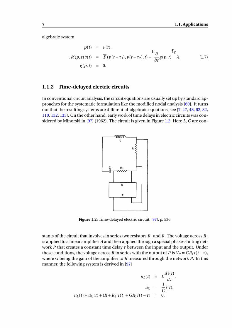
In conventional circuit analysis, the circuit equations are usually set up by standard ap-proaches for the systematic formulation like the modified nodal analysis [69]. It turnsout that the resulting systems are differential-algebraic equations, see [7, 47, 48, 62, 82,110, 132, 133]. On the other hand, early work of time delays in electric circuits was con-sidered by Minorski in [97] (1962). The circuit is given in Figure 1.2. Here L, C are con-
Figure 1.2: Time-delayed electric circuit, [97], p. 536.
stants of the circuit that involves in series two resistors R1 and R. The voltage across R1
is applied to a linear amplifier A and then applied through a special phase-shifting net-work P that creates a constant time delay τ between the input and the output. Underthese conditions, the voltage across R in series with the output of P is VP =GR1i (t −τ),where G being the gain of the amplifier to R measured through the network P . In thismanner, the following system is derived in [97]
uL(t ) = Ldi (t )
d t,
uC = 1
Ci (t ),
uL(t )+uC (t )+ (R +R1)i (t )+GR1i (t −τ) = 0,

1.1. Applications 8
which can be rewritten in the form of the linear DDAE0 0 L0 1 00 0 0
uL(t )uC (t )i (t )
=1 0 0
0 0 1C
1 1 R +R1
uL(t )uC (t )i (t )
+0 0 0
0 0 00 0 GR1
uL(t −τ)uC (t −τ)i (t −τ)
. (1.8)
Since the late 1960s, circuits which include delayed elements turn out to be popular inthe engineering community due to the fact that these circuits have a very importantrole due to the increase of performance of very large scale integration (VLSI) systems,[12, 21, 114–116]. The two typical types of circuits where delays usually occur are cir-cuits with transmission lines (TL) [21], and partial element equivalent circuits (PEEC’s)[114, 115]. These circuits result in neutral DDEs of the following form, see [12],
y(t ) = Ly(t )+M y(t −τ)+N y(t −τ), for all t ≥ t0, (1.9)
together with an initial function φ(t ). The delay τ> 0 is constant and t0 is the startingtime. For the solution procedure, directly applying numerical methods such as Runge-Kutta methods or multi-step methods requires an approximation of the derivative y(t−τ), which is a difficult task. The simple trick to overcome this difficulty is to introducea new functionΨ(t ) := y(t )−N y(t −τ) and to rewrite (1.9) as
Ψ(t ) = LΨ(t )+ (M +LN )y(t −τ),
y(t ) = Ψ(t )+N y(t −τ),
which in fact is the DDAE[I 00 0
][Ψ(t )y(t )
]=[
L 0I −I
][Ψ(t )y(t )
]+[
0 M +LN0 N
][Ψ(t −τ)y(t −τ)
].
Certainly, one may argue that this DDAE, which is reformulated from a neutral DDE,is quite artificial. However, the neutral DDE (1.9) is indeed a reduced system obtainedby neglecting certain variables and certain algebraic equations, using the Kirchhoff’svoltage law or the Kirchhoff’s current law. In general, the unreduced system, whichinvolves algebraic constraints obtained by these laws, is a delay differential-algebraicsystem.
1.1.3 DDAEs in fluid dynamics
The dynamical behavior of a system in fluid mechanics and turbulence modeling isoften described by the incompressible Navier-Stokes equation of the form
∂u
∂t−ν∆u +∇p + (u ·∇)u = f in (0,∞)×Ω,
∇·u = 0 in (0,∞)×Ω,
where ν > 0 is the viscosity, u = u(t ,ξ) is the velocity field which is a function of thetime t and the position ξ, p is the pressure, f is the external force. Recently, therehas been an increasing interest in the situation where the trajectories of some fluidparticles have a delay τ to follow the fluid [85, 104]. Furthermore, from the control
9 1.1. Applications
perspective, it is favorable to control the system by another external force g = g (t ,u(t−τ,ξ)) which involves some hereditary characteristics [34, 50]. This leads to the followingtime-delayed version of the incompressible Navier-Stokes equation
∂u∂t −ν∆u +∇p + (u(t −τ,ξ) ·∇)u = f + g (t ,u(t −τ,ξ)) in (0,∞)×Ω,
∇·u = 0 in (0,∞)×Ω,(1.10a)
together with the following initial and boundary conditions
u = 0 on (0,∞)×∂Ω,u(0, x) = u0(x) in Ω,u(t , x) = φ(t , x) in (−τ,0)×Ω.
(1.10b)
To obtain the numerical solution to the initial-boundary value problem (1.10), the fre-quently used method is to discretize the space variable by finite difference or finiteelement methods [57] and consequently one obtains a delay differential-algebraic sys-tem.
1.1.4 DDAEs in chemical engineering
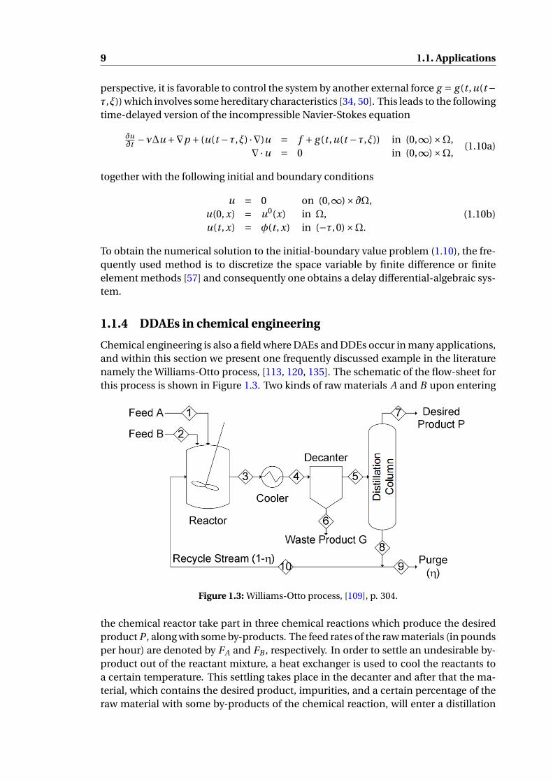
Chemical engineering is also a field where DAEs and DDEs occur in many applications,and within this section we present one frequently discussed example in the literaturenamely the Williams-Otto process, [113, 120, 135]. The schematic of the flow-sheet forthis process is shown in Figure 1.3. Two kinds of raw materials A and B upon entering
Figure 1.3: Williams-Otto process, [109], p. 304.
the chemical reactor take part in three chemical reactions which produce the desiredproduct P , along with some by-products. The feed rates of the raw materials (in poundsper hour) are denoted by FA and FB , respectively. In order to settle an undesirable by-product out of the reactant mixture, a heat exchanger is used to cool the reactants toa certain temperature. This settling takes place in the decanter and after that the ma-terial, which contains the desired product, impurities, and a certain percentage of theraw material with some by-products of the chemical reaction, will enter a distillation

1.1. Applications 10
column. There the valuable product is separated from the impurities, whereas the rawmaterial with the by-products is recycled to the chemical reactor to be reprocessed.The recycle loop, which ensures that useful products will not be discarded, introducesa significant time delay into the problem. In practical situations, it is not at all unusualfor material to take ten minutes to travel from the chemical reactor through the cooler,the decanter, the distillation column, and then recycling to the reactor. This is becauseof the distance separating the various stages of the overall process and lengths of pip-ing in the stages themselves.
Even though the originally proposed differential equation governing this chemical pro-cess is nonlinear, see [135], for the determination of a proper correction in the feedrates at the desired operating point, a corresponding linearized model is useful, see[113]. For a recycle time of ten minutes, the linearized equation describing the reac-tion in the chemical reactor is the following DDE with the delay τ= 10
x(t ) = A0x(t )+B0x(t −τ)+ f (t ), (1.11)
with
A0 =
−4.93 −1.01 0 0−3.20 −5.30 −12.8 06.40 0.347 −32.5 −1.04
0 0.833 11.0 −3.96
, B0 =
1.92 0 0 0
0 1.92 0 00 0 1.87 00 0 0 0.724
,
f (t ) = 1
6VR
1 00 10 00 0
[δFA
δFB
], x =
xA
xB
xC
xP
,
where VR is the volume of the chemical reactor (VR ≈ 2.628m3), δFA and δFB are thedeviations in the feed rates of the raw materials A and B , respectively, from their nomi-nal values. The dimensionless components xA, xB , xC and xP represent the deviationsfrom their nominal values in the weight compositions of the raw materials A and B ,of the intermediate product C , and of the desired product P , respectively. Note thatsix variables appear in [135] but the other two variables xG1 and xG2 correspond to thewaste product G , which does not react with the other chemicals, and so only the fourvariables given above occur in the DDE (1.11).
Furthermore, taking into account the mass conservation law, one obtains the followingalgebraic constraint
xA(t )+xB (t )+xG1 (t )+xG2 (t )+xC (t )+xP (t )
= g (t , xG1 (t −τ), xG2 (t −τ), xC (t −τ), xP (t −τ))+δFA +δFB ,(1.12)
where the scalar function g represents the weight of the recycled raw material with theby-products. The combined system (1.11)-(1.12) therefore gives rise to a DDAE in thevariable
x(t ) = [xA(t ) xB (t ) xG1 (t ) xG2 (t ) xC (t ) xP (t )]T
.
Chapter 2
Fundamentals of DAEs and DDEs
Before studying DDAEs, it is worthwhile to spend some time to recall the essentials ofthe theory of differential algebraic equations (DAEs) and of delay differential equations(DDEs) as well.The first part of this chapter, consisting of the first three sections, focuses on DAEs.In the first two sections, we recall the solvability analysis of first order systems, whichfollows by an extension to arbitrarily high order systems in the third section. In moredetail, the existence and uniqueness of a solution to a DAE is studied via the spectralanalysis (Section 2.1), or via the structure of the matrix function coefficients (Sections2.2 and 2.3).The second part of this chapter collects results on DDEs. Section 2.4 recalls importantfacts concerning the solution concept and the classification of different classes of time-delay equations. These have important consequences in the discontinuity propagationand the numerical integration of DDEs. We then present in Section 2.5 the method ofsteps, a standard tool for investigating the theoretical as well as the numerical solutionsto DDEs.
2.1 Time Invariant Differential-Algebraic Equations
In this section we consider time invariant differential-algebraic equations of the form
E x(t ) = Ax(t )+ f (t ). (2.1)
This equation (2.1) is obviously a special case of (1.2a) where the matrix function B isidentically zero, and the matrix functions E , A become constant matrices in Cm,n .
Definition 2.1. The matrix pair (E , A) in (Cm,n)2 is called regular if m = n and theso-called characteristic polynomial p(λ) defined by p(λ) = det(λE − A) is the non-zeropolynomial. Equivalently, the matrix pair (E , A) is regular if and only if the (finite) spec-trum σ(E , A) := λ ∈C | det(λE − A) = 0 is not the entire C.
Definition 2.2. A square matrix N ∈Cn,n is called nilpotent of nilpotency index ν= ν(N )if Nν = 0 and Nν−1 6= 0.
We recall one basic fact that the nilpotency index does not exceed the size of anilpotent matrix. Once the matrix pair (E , A) is regular, the solvability of (2.1) is char-acterized by using Kronecker-Weierstraß canonical form, see e.g., [26, 38].
11

2.1. Time Invariant Differential-Algebraic Equations 12
Theorem 2.3. (Kronecker-Weierstraß canonical form) Let E, A ∈ C n,n and (E , A) beregular. Then there exist nonsingular matrices W , T ∈Cn,n such that
(W ET, W AT ) =([
Id 00 N
],
[J 00 Ia
]), (2.2)
where N is a nilpotent matrix. Moreover, it is allowed that one or the other blocks is notpresent.
Definition 2.4. Consider a pair (E , A) of square matrices that is regular and has a canon-ical form as in (2.2). The quantity ν defined by
ν=
0 if the block N is absent in (2.2),
ν(N ) if N is present in (2.2),
is called the Kronecker index of the matrix pair (E , A) and is denoted by ν(E , A).
Definition 2.5. Let E ∈Cn,n and let ν= ν(E , I ) be the Kronecker index of the matrix pair(E , I ). A matrix X ∈Cn,n satisfying
E X = X E ,
X E X = X ,
X Eν+1 = Eν,
is called the Drazin inverse of E .
Clearly, the Kronecker index ν(E , I ) exists for every square matrix E , and it is zeroif and only if E is nonsingular. In this case, the Drazin inverse of E is nothing elsethan E−1. Otherwise, the existence and uniqueness of the Drazin inverse is given in thefollowing theorem.
Theorem 2.6. Let E ∈Cn,n and P be a nonsingular matrix such that
E = P
[C 00 N
]P−1,
where C is regular and N is nilpotent. Then,
E D = P
[C−1 0
0 0
]P−1.
Proof. For the proof, see [33].
Let λ0 be an arbitrary number such that the inverse of matrix λ0E − A exists, wedefine
E := (λ0E − A)−1E , A := (λ0E − A)−1 A, f := (λ0E − A)−1 f .
Making use of the Drazin inverse, one obtains the explicit representation for the solu-tion of (2.1) in the following theorem.
13 2.2. Time Varying Differential-Algebraic Equations
Theorem 2.7. Let the matrix pair (E , A) as in (2.1) be regular. Furthermore, let f ∈Cν(I,Cn) with ν is the Kronecker index of the matrix pair (E , A). Then every solutionx of the DAE (2.1) has the form
x(t ) = e E D At E D E x(0)+∫ t
0e E D A(t−s)E D E f (s)d s − (I − E D E)
ν−1∑j=0
(E AD ) j AD f ( j )(t ),
for all t ∈ I.
Proof. For the proof see Theorem 3.1.3, [26].
In the case that the matrix pair (E , A) is not regular, it is well-known that the cor-responding IVP for the DDAE (2.1) either has more than one solution or there are ar-bitrarily smooth inhomogeneities for which there is no solution at all, as presented inthe following theorem.
Theorem 2.8. Let (E , A) be as in (2.1) and suppose that (E , A) is a singular matrix pair.1. If rank(λE − A) < n for all λ ∈C, then the homogeneous initial value problem
E x(t ) = Ax(t ), x(0) = 0,
has a nontrivial solution.2. If rank(λE − A) = n for some λ ∈ C and hence m > n, then there exist arbitrarilysmooth inhomogeneities f for which the corresponding differential-algebraic equationis not solvable.
Proof. For the proof see Theorem 2.14, [75].
2.2 Time Varying Differential-Algebraic Equations
As we have seen in Section 2.1, the solvability analysis of the time invariant DAE (2.1)is characterized by the structure of the matrix pair (E , A). The aim of this section is tostudy linear time varying coefficients DAEs of the form
E(t )x(t ) = A(t )x(t )+ f (t ), for all t ∈ I, (2.3a)
x(0) = x0, (2.3b)
by analyzing the structure of the matrix function pair (E , A). To do that, we shall slightlymodify the algebraic approach [75] by transforming system (2.3a) only from the left.The reason for choosing this approach is that it is suitable for not only uniquely solv-able DAEs, but also for over- and under-determined DAEs, which is an important ad-vantage for our study of DDAEs later.The solution concept for DAEs of the form (2.3a) is stated in the next definition.
Definition 2.9. A function x : I→Cn is called:i) a (classical) solution of (2.3a) if x ∈C 1(I,Cn) and x satisfies (2.3a) pointwise,
ii) a (classical) solution of the IVP (2.3) if x is a solution of (2.3a) and satisfies (2.3b).
2.2. Time Varying Differential-Algebraic Equations 14
An initial vector x0 is called consistent to system (2.3a) if the IVP (2.3) has a solution.System (2.3a) is called solvable if it has at least one solution. It is called regular if inaddition, for any consistent initial vector x0, the corresponding IVP (2.3) has a uniquesolution.
We will make frequent use of the following results, compare Theorems 3.9, 3.25 in[75].
Theorem 2.10. Let E ∈C`(I,Cm,n), ` ∈N0∪∞, with constant rankE(t ) = r for all t ∈ I.Then there exist pointwise unitary functions U ∈ C`(I,Cm,m) and V ∈ C`(I,Cn,n), suchthat
U H EV =[Σ 00 0
], or U H E =
[E1
0
],
with pointwise nonsingular Σ ∈C`(I,Cr,r ), and E1 has full row rank r .
Theorem 2.11. Let I⊂ R be a closed interval and M ∈C (I,Cm,n). Then there exist openintervals I j ⊂ I, j ∈N, with⋃
j∈NI j = I, Ii ∩I j =; for i 6= j ,
and integers r j ∈N0, j ∈N such that
rank M(t ) = r j for all t ∈ I j .
Lemma 2.12. For the pair (P,Q) with P ∈C`(I,Cp,n), Q ∈C k (I,Cq,n), `, k ∈N0∪∞, as-
sume that there exist two integers rQ 6 r[P ;Q] such that rankQ(t ) = rQ and rank
[P (t )Q(t )
]=
r[P ;Q] for all t ∈ I. Then, there exists
[S 0Z1 Z2
]∈C min`,k(I,Cp,p+q ) that satisfies the fol-
lowing conditions.
i)
[SZ1
]∈C (I,Cp,p ) is pointwise unitary,
ii) Z1P +Z2Q = 0,iii) the function SP has pointwise full row rank, and the pair (SP,Q) satisfies
rank
([SPQ
])= rank(SP )+ rank(Q).
Proof. Since Q has constant rank on I, one can apply Theorem 2.10 to factorize Q, andthen partition P conformably to getIp 0
0 U H11
0 U H12
[PQ
][V11 V12
]=P1 P2
Σ 00 0
prQ
q − rQ
, (2.4)
where U1 =[U11 U12
] ∈C k (I,Cq,q ), V1 =[V11 V12
] ∈C k (I,Cn,n) are pointwise unitaryfunctions, and Σ ∈C k (I,CrQ ,rQ ) is pointwise nonsingular. The sizes of the block rows in
15 2.2. Time Varying Differential-Algebraic Equations
(2.4) are p, rQ , q − rQ . Moreover, note that in (2.4), P2 also has constant rank due to
rank(P2) = rank
([Ip 00 U H
1
][PQ
][V11 V12
])− rank(Σ) = r[P ;Q] − rQ .
Then, by Theorem 2.10, there exists a pointwise unitary function
U H2 =[
SZ1
]∈C min`,k(I,Cp,p ) such that
U H2 P2 =
[SZ1
]P2 =
[P12
0
], (2.5)
where P12 ∈C min`,k (I,Cr[P ;Q]−rQ ,n−rQ ) has pointwise full row rank.Combining (2.4) and (2.5), one obtains
S 0Z1 00 U H
110 U H
12
[
PQ
][V11 V12
]=
P11 P12
P21 0Σ 00 0
r[P ;Q] − rQ
p − r[P ;Q] + rQ
rQ
q − rQ
,
where P12 has pointwise full row rank and Σ is pointwise nonsingular on I.Consequently, SP = [P11 P12
]V −1
1 has pointwise full row rank. Moreover, one seesthat
rank
([SPQ
])= rank
([P11 P12
Σ 0
])= rank
([0 P12
])+ rank([Σ 0
])= rank(SP )+ rank(Q).
Since Σ ∈ C k (I,CrQ ,rQ ) is pointwise nonsingular, it implies that Σ−1 ∈ C k (I,CrQ ,rQ ). Fi-nally, setting Z2 :=−P21Σ
−1U H11 ∈C min`,k(I,Cp−r[P ;Q]+rQ ,q ), we obtain
Z1P +Z2Q = ([P21 0]−P21Σ−1[Σ 0]
)V −1
1 = 0,
which completes the proof.Following the algebraic approach [75], we rewrite equation (2.3a) in the form(
E(t )d
dt− A(t )
)x(t ) = f (t ), (2.6)
for any t ∈ I. For notational convenience, we will omit the time variable t in all matrixfunctions.Making use of Theorem 2.11 and restricting ourselves if necessary to subintervals, wemay assume that the following assumption holds.
Assumption 2.13. For the pair of matrix functions (E , A) of the DAE (2.3a), there existintegers r, a such that
rank(E) = r, rank([
E A])= r +a
for all t ∈ I.

2.2. Time Varying Differential-Algebraic Equations 16
Lemma 2.14. Consider the DAE (2.3a) and suppose that Assumption 2.13 holds. Then,there exists a pointwise unitary function P1 ∈C (I,Cm,m) such that by scaling system (2.6)with P1 from the left one obtains a new system in the following formM11
ddt −M12
−M22
0
x = f1
f2
f3
rav
, (2.7)
where the functions M11 ∈C (I,Cr,n), M22 ∈C (I,Ca,n) have pointwise full row rank. Herethe sizes of the block row equations are r, a and v = m − r −a.
Proof. First we determine a pointwise unitary function PE : I→Cm,m via Theorem 2.10or a smooth QR-decomposition, see [39], that compresses the matrix function E . Thisyields
PE
(E
d
dt− A
)=[
M11d
dt −M12
−M22
]r
m − r,
such that M11 has full row rank. Continuing, by compressing the block M22 with apointwise unitary function P A : I→Cm−r,m−r , this yields
[Ir 00 P A
]PE
(E
d
dt− A
)=[
Ir 00 P A
][M11
ddt −M12
−M22
]=M11
ddt −M12
−M22
0
,
where M11 and M22 have pointwise full row rank. Setting P1 :=[
Ir 00 P A
]PE , we arrive
at (2.7).
The formula (2.7) in Lemma 2.14 clearly shows that the number of scalar (nontriv-ial) differential equations in system (2.3a) is r , while the number of scalar (nontrivial)algebraic constraints is a.
In the following we suppose that the function M22 is continuously differentiable. Again,to be able to apply Lemma 2.12, the following assumption is necessary.
Assumption 2.15. For the DAE (2.7), there exists m ∈N such that the functions M11, M22
satisfy
rank
([M11
M22
])= m, for all t ∈ I.
Under Assumption 2.15, applying Lemma 2.12 to the pair (M11, M22) implies theexistence of matrix functions S, Z1, Z2 of appropriate sizes that have the followingproperties
i) the function
[SZ1
]∈C (I,Cr,r ) is pointwise unitary,
ii) the function SM11 has pointwise full row rank and the following identities hold:
Z1M11 = Z2M22, (2.8)

17 2.2. Time Varying Differential-Algebraic Equations
and
rank
([SM11
M22
])= rank(SM11)+ rank(M22).
Define the operator
P2 :=
S 0 0Z1 Z2
ddt 0
0 Ia 00 0 Iv
dsav
, (2.9)
where r = d + s, we see that P2 has a left-inverse given by the formula
P−12 =
[
SZ1
]−1
−[
SZ1
]−1[0
Z2d
dt
]0
0 Ia 00 0 Iv
d + s
av
.
Applying the operator P2 to system (2.7), we obtainS 0 0Z1 Z2
ddt 0
0 Ia 00 0 Iv
M11
ddt −M12
−M22
0
x =
S 0 0Z1 Z2
ddt 0
0 Ia 00 0 Iv
f1
f2
f3
dsav
,
or equivalently,SM11
ddt −SM12
Z1M11d
dt −Z1M12 −Z2d
dt M22
−M22
0
x =
S f1
Z1 f1 +Z2 f2
f2
f3
dsav
. (2.10)
According to ddt M22 = M22 +M22
ddt and (2.8), it follows that the second block equation
of (2.10) becomes (−Z1M12 −Z2M22)
x = Z1 f1 +Z2 f2.
As a result, (2.10) becomesSM11
ddt −SM12
−Z1M12 −Z2M22
−M22
0
x =
S f1
Z1 f1 +Z2 f2
f2
f3
dsav
. (2.11)
It is worth to note that the existence of the left-inverse P−12 of P2 guarantees that the
step of transforming system (2.6) via (2.7) to (2.11) does not alter the solution set of sys-tem (2.6). Furthermore, the number of scalar differential equations has been reducedfrom r to d . Continuing this reduction process leads us to the following algorithm.

2.2. Time Varying Differential-Algebraic Equations 18
Algorithm 2.1 Reformulation algorithm for the DAE (2.3a)
1: Set i = 0 and let E 0 = E , A0 = A, f 0 = f , r 0 = r , a0 = a.2: Determine a pointwise unitary function P1 as in Lemma 2.14 to bring the DAE(
E i ddt − Ai
)x = f i to the formM11
ddt −M12
−M22
0
x = f1
f2
f3
r i
ai
v i, (2.12)
where the functions M11, M22 have pointwise full row rank.
3: if rank[M T
11 M T22
]T = r i +ai then STOP with the resulting system (2.12),4: else proceed to 5.5: Determine the operator P2 as in (2.9) and apply it to system (2.12) results in
SM11d
dt −SM12
−Z1M12 −Z2M22
−M22
0
x =
S f1
Z1 f1 +Z2 f2
f2
f3
d i
si
ai
v i
.
6: Increase i by 1, set
E i :=
SM11
000
, Ai :=
SM12
Z1M12 +Z2M22
M22
0
, f i =
S f1
Z1 f1 +Z2 f2
f2
f3
,
and repeat the process from 2.7: end if
Since r i+1 = r i − si , Algorithm 2.1 terminates after a finite number of iterations. Thisguarantees the existence of the so-called strangeness index of the DAE (2.3a) definedby µ= mini ∈N0, r i = r i+1. We also call µ the strangeness index of the pair (E , A).
Theorem 2.16. Consider the DAE (2.3a) and assume that its strangeness index µ is welldefined. Then, the DAE (2.3a) has the same solution set as the resulting DAE, which wedenote by M11
ddt − M12
−M22
0
x =
f1
f2
f3
,dµ
aµ
vµ(2.13)
where
[M11
M22
]has pointwise full row rank. The functions f2, f3 depend on f , f , . . . , f (µ),
while the function f1 depends only on f .
The quantities dµ, aµ, vµ and uµ := n −dµ− aµ are called the characteristic quan-tities of the DAE (2.3a). In particular, uµ is the number of undetermined variables con-tained in the state vector-valued function x. Following the notation in [75], we also call(2.13) the strangeness-free formulation of the DAE (2.3a).

19 2.2. Time Varying Differential-Algebraic Equations
As a direct result, the solvability of the DAE (2.3a) is analyzed in the following corollary.
Corollary 2.17. Consider the DAE (2.3a) and assume that its strangeness index µ is welldefined. Then, the following assertions hold.i) The DAE (2.3a) is solvable if and only if in (2.13), one has either f3 = 0 or vµ = 0.ii) The initial condition x0 is consistent if and only if in addition, −M22(0)x0 = f2(0). Inthis case, (2.3a) has the same solution set as the underlying linear system[
M11
−M22
]x =[
M12˙M22
]x +[
f1˙f2
]. (2.14)
iii) Furthermore, (2.3a) is regular if and only if in addition uµ = 0. If this is the case,(2.14) becomes an ODE, which is often called an underlying ODE in the literature, see[6, 22, 82].
Remark 2.18. Whereas other index concepts, such as differentiation index [22], per-turbation index [66], or tractability index [82], aiming at the resulting system is ei-ther an underlying ODE or an inherent ODE, the goal of the strangeness index is thestrangeness-free formulation (2.13) and the underlying linear system (2.14). Conse-quently, the strangeness index is suitable for general DAEs, which can be underdeter-mined or overdetermined.
The validity of Algorithm 2.1 is illustrated by the next example.
Example 2.19. We apply Algorithm 2.1 to the following DAE[−t t 2
−1 t
]x +[
1 00 1
]x =[
00
]. (2.15)
First scaling the system with P1 =[
0 −1−1 t
]yields system (2.12)
[ ddt −t d
dt −1−1 t
]x =[
00
]. (2.16)
Then, applying the operator
P2 =[
1 ddt
0 1
]to (2.16) using d
dt t = 1+ t ddt , we obtain the strangeness-free formulation (2.13)[
0 0−1 t
]x =[
00
].
The strangeness-index is µ = 1, and the characteristic invariants are dµ = 0, aµ = 1,vµ = 1, uµ = 1.
In order to understand the effect of the reformulation procedure performed in Al-gorithm 2.1 to DDAEs, we apply it to a modification of the DAE (1.3) including a func-

2.2. Time Varying Differential-Algebraic Equations 20
tion parameter that reads
E(t )x(t ) = A(t )x(t )+T (t )λ(t )+ f (t ), (2.17a)
together with an initial vectorx(0) = x0. (2.17b)
Here λ : I→Cn and T : I→Cm,n . We further assume that E , A, T and f are sufficientlysmooth.The smoothness comparison between the function parameter λ and the state variablex gives rise to the system classification as follows.
Definition 2.20. The parameter dependent DAE (2.17a) is called:i) retarded if for any continuous function λ, there exists a solution x to the IVP
(2.17). Since the solution x is continuously differentiable, formally, we will say xis smoother than λ.
ii) neutral if for any continuously differentiable function λ, there exists a solution xto the IVP (2.17). Formally, we will say x is at least as smooth as λ.
iii) The remaining case, where λ must be at least two times continuously differen-tiable to guarantee the existence of a solution x to (2.17), is called advanced.
This classification leads to different forms of the resulting DAE (2.13) as in the fol-lowing lemma.
Lemma 2.21. Suppose that the parameter dependent DAE (2.17a) is not advanced andthe strangeness index µ is well-defined for the function pair (E , A) of (2.17a). Consid-ering T (t )λ(t )+ f (t ) as a new inhomogeneity, then Algorithm 2.1 applied to (2.17a)results in a systemE1(t )
00
x(t ) =A1(t )
A2(t )0
x(t )+T 0
1 (t )T 0
2 (t )T 0
3 (t )
λ(t )+ 0
0T 1
3 (t )
λ(t )+
f1(t )f2(t )f3(t )
, (2.18)
where the matrix function
[E1
A2
]is of pointwise full row rank. In addition, if (2.17a) is of
retarded type then T 02 = 0 and T 1
3 = 0.
Proof. When applying the strangeness-free formulation to the DAE (2.17a), the as-sumption that the system is not advanced ensures that all algebraic constraints of(2.17a) have the form
0 = A2(t )x(t )+ T2(t )λ(t )+ f2(t ),
for some matrix functions A2, T2, f2. On the other hand, all differential equations of(2.17a) have the form
E1(t )x(t ) = A1(t )x(t )+ T1(t )λ(t )+ f1(t ),
for some matrix functions E1, A1, T1, f1. Moreover, consistency conditions for λ andfor the inhomogeneity of the DAE (2.17a) can only arise from one of the following threesources:

21 2.3. High-order Differential-Algebraic Equations
i) Adding an algebraic equation to another algebraic equation;ii) Adding a differential equation to another differential equation;
iii) Adding the derivative of some algebraic equation to a differential equation.Therefore, the consistency condition for the inhomogeneity of (2.17a) does not containderivatives of λ of order bigger than one. This means that Algorithm 2.1 applied to(2.17a) results in the DAE of the form (2.18).
2.3 High-order Differential-Algebraic Equations
As will be seen later in Example 3.5, even though the DDAE (1.2a) is of first order, itis necessary to study high-order DAEs, since a first order DDAE may contain a hiddenhigh-order DAE. Therefore, in this section we discuss high-order DAEs of the form
Ak (t )x(k)(t )+·· ·+ A1(t )x(t )+ A0(t )x(t ) = f (t ), (2.19a)
on the time interval t ∈ I = [0, t f ) ⊂ R, where Ai : I → Cm,n , for i = 1, . . . ,k, Ak 6= 0,and f : I→ Cm . Similar to the first order case, we investigate the solvability of an IVPconsisting of (2.19a) and the initial conditions
x(k−1)(0) = x(k−1)0 , . . . , x(0) = x0, x(0) = x0. (2.19b)
The solution concept for high-order DAEs of the form (2.19a) is stated in the next defi-nition.
Definition 2.22. A function x : I→Cn is calledi) a (classical) solution of (2.19a) if x ∈C k (I,Cn) and x satisfies (2.19a) pointwise,ii) a (classical) solution of the IVP (2.19) if x is a solution of (2.19a) and satisfies (2.19b).We introduce X0 := [x(k−1),T
0 · · ·xT0 ]T ∈Ckn as an initial vector of the IVP (2.19).
iii) An initial vector X0 is called consistent to system (2.19a) if the IVP (2.19) has a solu-tion.iv) System (2.19a) is called solvable if it has at least one solution. It is called regular ifit is solvable and for any consistent initial vector X0, the corresponding IVP (2.19) hasa unique solution.
First order DAEs (k = 1) play a crucial role in various applications in science and en-gineering. Numerous investigations including both theoretical and numerical aspectsare well known, see [6, 22, 75] and references therein. Another case of (2.19a) wherek = 2 arise in various applications, ranging from constrained mechanical systems, seee.g. [43, 53, 99, 108], to electrical and electro-mechanical systems [8, 9], heterogeneoussystems [102], and traveling waves [32, 89], etc.
Even though special cases (k = 1, 2) of system (2.19a) are considered, there are notmany available results about the general case, see [93]. More important, it has beenobserved, see e. g., [3, 93, 117, 123, 139] that the classical approach of ordinary differ-ential equations, which transforms system (2.19a) into a first order DAE by introducingnew variables that represent derivatives of x(t ), may lead to a number of mathemat-ical difficulties, for example, unnecessary requirements on the smoothness of the in-homogeneity, or even failure of numerical methods applied to a resulting first ordersystem. The direct treatment for (2.19a) therefore aims at a suitable reformulation that

2.3. High-order Differential-Algebraic Equations 22
not only leads to an underlying equation but also reveals all the hidden constraintscontained in (2.19a). This goal is achieved by using an algebraic method, for detailssee [93, 123, 139, 140]. Another way to deal with (2.19a), in the same spirit as [75], is toextend Algorithm 2.1 to high-order systems, see e.g. [63]. There, the strangeness indexconcept is also generalized for arbitrarily high order DAEs. However, in order to main-tain the conciseness and clarity of this thesis, the detailed proof will be omitted.
In the following theorem, by the term appropriate constant rank assumptions wemean all the requirements that some matrix-valued function must have constant rankon the time interval I. From Theorem 2.11, we know that these requirements hold lo-cally, except for a countable set of points in I.
Theorem 2.23. Consider the DAE (2.19a). Then, under appropriate constant rank as-sumptions, the DAE (2.19a) has the same solution set as the so-called strangeness-freeDAE
Ak,1 Ak−1,1 . . . A0,1
Ak−1,2 . . . A0,2. . .
...A0,k+1
0 0 . . . 0
x(k)
x(k−1)
...x
=
f1
f2...
fk+1
fk+2,
rk
rk−1...
r0
v
(2.20)
where the matrix-valued function[
ATk,1 . . . AT
0,k+1
]Thas pointwise full row rank. The
number of undetermined variables contained in the state function x is u = n −∑ki=0 ri .
In analogy to the case of first order systems, the quantities rk , . . . ,r0, v,u are called thecharacteristic quantities of the DAE (2.19a).
To deduce the underlying linear system from the strangeness-free DAE (2.20), weneed the following lemma.
Lemma 2.24. Given a function F (t ) on the time interval I = [0, t f ), and assume that Fis i times continuously differentiable and satisfies the following conditions
F ( j )(0) = 0, for j = 0, . . . , i .
Then the following equations are equivalent:
i) F (t ) = 0 for all t ∈ [0, t f ).ii) F (i )(t ) = 0 for all t ∈ [0, t f ).
Proof. The proof can be simply obtained by induction via the identities
F ( j−1)(t ) = F ( j )(0)+∫ t
0F ( j )(s)d s,
for j = i , . . . ,1.
Using Lemma 2.24, in the next corollary we derive the underlying linear system
23 2.3. High-order Differential-Algebraic Equations
from (2.20) if the following consistency conditions hold(d
dt
)i (Ak−1,2x(k−1)(t )+·· ·+ A1,2x(1)(t )+ A0,2x(t )− f2(t )
)∣∣∣t=0
= 0, i = 0,1,
. . . (2.21)(d
dt
)i (A0,k+1x(t )− fk+1(t )
)∣∣∣t=0
= 0, i = 0, . . . ,k,
fk+2 = 0.
Corollary 2.25. Consider the DAE (2.19a) and its reformulated system (2.20). Moreover,suppose that the consistency condition (2.21) is satisfied. Then, (2.19a) has the samesolution set as the underlying linear system
Ak,1 ∗ . . . ∗ ∗Ak−1,2 ∗ . . . ∗ ∗
... ∗ . . . ∗ ∗A1,k ∗ . . . ∗ ∗
A0,k+1 ∗ . . . ∗ ∗
x(k)
x(k−1)
...x(1)
x
=
f1
f (1)2...
f (k−1)kf (k)
k+1
. (2.22)
Here the leading matrix function[
ATk,1 . . . AT
0,k+1
]Thas pointwise full row rank, and
by ∗ we denote non-specified matrix functions of appropriate sizes.
Proof. The formula (2.22) can be directly obtained from the strangeness-free DAE (2.20)by differentiating the i th-block equation exactly i−1 times. Furthermore, due to Lemma2.24, the two systems (2.20) and (2.22) have the same solution set, provided that theconsistency condition (2.21) holds.
The following corollary is a direct consequence of Theorem 2.23.
Corollary 2.26. Consider the DAE (2.19a) and its reformulated system (2.20). Then wehave:i) The DAE (2.19a) is solvable if and only if either 0 = fk+2 or v = 0.
ii) The initial vector X0 =[
x(k−1),T0 · · · xT
0
]Tis consistent if and only if in addition the
following identity holdsAk−1,2(0) Ak−2,2(0) . . . A0,2(0)
Ak−2,3(0) . . . A0,3(0). . .
...A0,k+1(0)
x(k−1)0
x(k−2)0
...x0
=
f2(0)f3(0)
...fk+1(0)
.
iii) The IVP (2.19) is regular if and only if in addition, u = 0. If this is the case, the linearsystem (2.22) becomes an ODE, and we also call it an underlying ODE of the DAE (2.19a).
After collecting results about DAEs, within the next subsection we present someimportant facts of DDEs.
2.4. Classification of DDEs 24
2.4 Classification of Delay Differential Equations
As will be seen later, DDAEs of the form (1.2a) contains many types of DDEs, ratherthan only the DDE (1.4). Since these types of DDEs lead to different solution concepts,a classification of time-delayed systems is necessary. This matter was first mentionedin [15], where the authors studied the scalar equation with a single delay
a0x(t )+a1x(t −τ)+b0x(t )+b1x(t −τ) = f (t ). (2.23)
An equation of the form (2.23) is said to be of retarded type if a0 6= 0 and a1 = 0, neutraltype if a0 6= 0 and a1 6= 0, advanced type if a0 = 0, b0 6= 0 and a1 6= 0.Clearly, x(t ) is smoother (resp., less smooth) than x(t −τ) if (2.23) is of retarded (resp.advanced) type. In the case of neutral type, x(t ) is as smooth as x(t −τ). This classi-fication can be directly generalized for high order, high dimensional linear DDEs withmultiple delays of the following form
K+∑β=0
Gβ(t )x(β)(t ) =K−∑α=0
Hα(t )x(α)(t −−→τ )+ f (t ). (2.24)
Here −→τ := [τ1 . . . τh]
is an h-dimensional delay vector that satisfies 0 < τ1 < ·· · < τh.The n-dimensional function x describes the behaviour of a process in the time interval
I, and by x(t −−→τ ) we mean the hn dimensional vector[xT (t −τ1) . . . xT (t −τh)
]T.
We further assume that the matrix function GK+ is pointwise invertible and the func-tion HK− is not identically zero. Based on the comparison between K+ and K−, DDEsof the form (2.24) can be categorized into three following types:i) retarded if K+ > K−. The following equation is an example of a retarded DDE
x(t ) = x(t )+x(t −1)+ f (t ).
ii) neutral if K+ = K−. The following equation is an example of a neutral DDE
x(t ) = x(t )+x(t −1)+ x(t −1)+ f (t ).
iii) advanced if K+ < K−. The following equation is an example of an advanced DDE
x(t ) = x(t )+x(t −1)+ x(t −1)+ f (t ).
Remark 2.27. It should be noted that these three classes of DDEs (retarded, neutraland advanced) are in fact very different. Each class possesses its own features, rang-ing from basic properties such as a solution concept, the discontinuity propagation ofthe solution, smoothness requirements for an initial function, to critical control issuessuch as stability, controllability and observability, see e.g. [13, 15, 95].
Systems with multiple constant delays can be further classified. Delays whose quo-tients are rational are called commensurate delay, [54, 111]. For example, the delays ofthe system
x(t ) = x(t )+x(t −1)+x(t −p2)
are non-commensurate. In particular, for −→τ = [τ0 2τ0 . . . hτ0]
with some h ∈ N,
25 2.5. Solution concepts and the method of steps for DDEs
the linear commensurate delay DDE
x(t ) = H0x(t )+H1x(t −−→τ ),
has been intensively discussed in the literature, see e.g., [13, 15, 54, 67].
Remark 2.28. In general, the delay −→τ can also depend on the time variable t (timedependent delay) and the state x (state dependent delay). These cases have also beenthoroughly studied in the theory of DDEs, see e.g., [13, 15, 67]. However, within thisthesis, we do not discuss these cases.
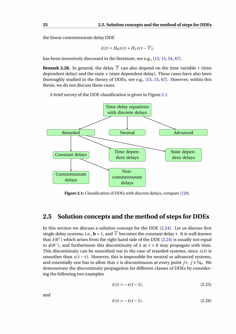
A brief survey of the DDE classification is given in Figure 2.1.
Time delay equationswith discrete delays
NeutralRetarded Advanced
Constant delaysTime depen-dent delays
State depen-dent delays
Commensuratedelays
Non-commensurate
delays
Figure 2.1: Classification of DDEs with discrete delays, compare [120].
2.5 Solution concepts and the method of steps for DDEs
In this section we discuss a solution concept for the DDE (2.24). Let us discuss firstsingle delay systems, i.e., h = 1, and −→τ becomes the constant delay τ. It is well-knownthat x(0+) which arises from the right hand side of the DDE (2.24) is usually not equalto φ(0−), and furthermore this discontinuity of x at t = 0 may propagate with time.This discontinuity can be smoothed out in the case of retarded systems, since x(t ) issmoother than x(t −τ). However, this is impossible for neutral or advanced systems,and essentially one has to allow that x is discontinuous at every point jτ, j ∈ N0. Wedemonstrate the discontinuity propagation for different classes of DDEs by consider-ing the following two examples
x(t ) =−x(t −1), (2.25)
andx(t ) =−x(t −1). (2.26)

2.5. Solution concepts and the method of steps for DDEs 26
−1 0 1 2 3 4
−0.5
0
0.5
1
x
−1 0 1 2 3 4−1.2
−1
−0.8
−0.6
−0.4
−0.2
0
0.2
x
Figure 2.2: Discontinuity propagation of the solutions to (2.25) (left) and (2.26) (right).
Figure 2.2 clearly shows that x becomes smoother in the retarded case ((2.25)) and xretains the smoothness of φ in the neutral case ((2.26)). Consequently, for (2.26), x doesnot exist at the points 0, τ, 2τ, . . . . To deal with this property, the concept of piecewisedifferentiable solution is usually used for neutral and advanced DDEs, see e.g. [13, 95],i.e., the function x that fulfills (2.24) at almost every point of I.
In the general case where h ≥ 2, it has been proved, see [15], that if an initial functionφ is sufficiently smooth on [−τ,0], then the set of discontinuities (of the solution x to(2.24) and of its derivatives) is a subset of < β,−→τ >, β ∈Nh. This means that withoutcomputing the solution to (2.24), one already knows all the possible discontinuitiespoints of DDEs beforehand.
Now let us consider the smoothness requirement for an initial function so that the cor-responding IVP for the DDE (2.24) has a solution. Clearly, if (2.24) is of retarded type(K− < K+) then the smoothness condition for φ is that φ ∈ C K−([−τh,0]). In the caseof neutral type, the sufficient condition is that φ ∈ C K+([−τh,0]). In the last case, foradvanced DDEs of the form (2.24), we see that x(t ) is K+−K− times less smooth thanx(t −τ). Thus, the smoothness requirement depends on the length of the time intervalI. In particular, if I is unbounded then typically φ must be infinitely smooth.
For DDEs, the so-called method of steps (or method of successive integration) is a stan-dard tool to investigate the analytical and numerical solutions [13, 14, 16, 17]. To illus-trate this method we shall apply it to the DDE (2.24).
Since τ1 = minτi | 1 6 i 6 h, we introduce sequences of matrix-valued and vector-valued functions on the time interval [0,τ1] as follows
Gβ,i (t ) := Gβ(t + (i −1)τ1),
gi (t ) :=K−∑α=0
Hα(t + (i −1)τ1)x(α)(t + (i −1)τ1 −−→τ )+ f (t + (i −1)τ1),
xi (t ) := x(t + (i −1)τ1),
for β = 1, . . . ,K+, i = 1, 2, . . . and t ∈ [0,τ1]. The function xi (resp. fi ) should be inter-preted as the restriction on the time interval [(i −1)τ1, iτ1] of x (resp. f ). In this way

27 2.5. Solution concepts and the method of steps for DDEs
the DDE (2.24) is rewritten as a sequence of ODEs on the time interval [0,τ1]
K+∑β=0
Gβ,i (t )x(β)i (t ) = gi (t ), (2.27)
for all t ∈ (0,τ1), i = 1, 2, . . . . The pointwise invertibility of the function GK+ implies thatGK+,i is also invertible for any i .Assuming that the solution x of (2.24) is already solved on the time interval [0, (i−1)τ1],we then want to determine x on [(i −1)τ1, iτ1].Since t+(i−1)τ1−τ j < (i−1)τ1 for all j = 1, . . . ,h and t ∈ [0,τ1], we see that the functiongi is already known and hence, (2.27) is nothing else than an ODE of the variable xi .Furthermore, to obtain a unique solution xi of (2.27), we still need to specify the initialconditions xi (0), . . . , x(K+−1)
i (0). One possible option for this is to utilize the continuityof the functions x, . . . , x(K+−1) at the point iτ1, i.e.,
x( j )i (0) := lim
t↑τx( j )
i−1(t ), j = 0, . . . ,K+−1.
Therefore, the desired solution x is found on successive intervals [(i −1)τ1, iτ1], i ≥ 1by solving the ODE (2.27) for each i = 1,2, . . . . In this way, a piecewise differentiablesolution of (2.24) exists and is unique on I, provided that a sufficiently smooth initialfunction φ is specified.
Remark 2.29. In the single delay case, the ODE (2.27) takes the following form
K+∑β=0
Gβ,i (t )x(β)i (t ) =
K−∑α=0
Hα(t + (i −1)τ1)x(α)i−1(t )+ f (t + (i −1)τ1).
Remark 2.30. In most applications encountered in science and engineering, the timedelay system is of either retarded or neutral type, [40, 46, 56, 74, 95, 126, 134]. Fromanother viewpoint, for the numerical integration of DDEs, the numerical solutions areoften computed based on Taylor expansions, and consequently this makes sense onlyif the analytical solution is assumed to be sufficiently smooth up to some order. How-ever, for advanced DDEs, the function xi = x|[(i−1)τ,iτ] is always less smooth than theprevious function xi−1 = x|[(i−2)τ,(i−1)τ] and the Taylor series may not exist for some i .For this reason the numerical solution of DDEs has been studied mostly for equationsof retarded and neutral type. Until now, there is still a lack of a systematic theory foradvanced DDEs, the references are rare and limited to only few special applications[36, 73, 106].

2.5. Solution concepts and the method of steps for DDEs 28
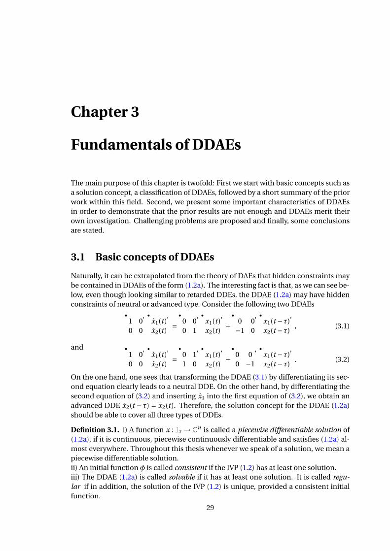
Chapter 3
Fundamentals of DDAEs
The main purpose of this chapter is twofold: First we start with basic concepts such asa solution concept, a classification of DDAEs, followed by a short summary of the priorwork within this field. Second, we present some important characteristics of DDAEsin order to demonstrate that the prior results are not enough and DDAEs merit theirown investigation. Challenging problems are proposed and finally, some conclusionsare stated.
3.1 Basic concepts of DDAEs
Naturally, it can be extrapolated from the theory of DAEs that hidden constraints maybe contained in DDAEs of the form (1.2a). The interesting fact is that, as we can see be-low, even though looking similar to retarded DDEs, the DDAE (1.2a) may have hiddenconstraints of neutral or advanced type. Consider the following two DDAEs[
1 00 0
][x1(t )x2(t )
]=[
0 00 1
][x1(t )x2(t )
]+[
0 0−1 0
][x1(t −τ)x2(t −τ)
], (3.1)
and [1 00 0
][x1(t )x2(t )
]=[
0 11 0
][x1(t )x2(t )
]+[
0 00 −1
][x1(t −τ)x2(t −τ)
]. (3.2)
On the one hand, one sees that transforming the DDAE (3.1) by differentiating its sec-ond equation clearly leads to a neutral DDE. On the other hand, by differentiating thesecond equation of (3.2) and inserting x1 into the first equation of (3.2), we obtain anadvanced DDE x2(t −τ) = x2(t ). Therefore, the solution concept for the DDAE (1.2a)should be able to cover all three types of DDEs.
Definition 3.1. i) A function x : Iτ → Cn is called a piecewise differentiable solution of(1.2a), if it is continuous, piecewise continuously differentiable and satisfies (1.2a) al-most everywhere. Throughout this thesis whenever we speak of a solution, we mean apiecewise differentiable solution.ii) An initial function φ is called consistent if the IVP (1.2) has at least one solution.iii) The DDAE (1.2a) is called solvable if it has at least one solution. It is called regu-lar if in addition, the solution of the IVP (1.2) is unique, provided a consistent initialfunction.
29

3.1. Basic concepts of DDAEs 30
The solvability analysis of DAEs considered in Sections 2.2-2.3 motives the conceptof the strangeness-free formulation for the DDAE (1.2a) in the following definition.
Definition 3.2. Consider the DDAE (1.2a). A system of the formAµ,1 Aµ−1,1 . . . A0,1
Aµ−1,2 . . . A0,2. . .
...A0,µ+1
0 0 . . . 0
x(µ)(t )x(µ−1)(t )
...x(t )
=
Bη,1 Bη−1,1 . . . B0,1
Bη,2 Bη−1,2 . . . B0,2...
......
Bη,µ+1 Bη−1,µ+1 . . . B0,µ+1
Bη,µ+2 Bη−1,µ+2 . . . B0,µ+2
x(η)(t −τ)x(η−1)(t −τ)
...x(t −τ)
+
f1
f2...
fµ+1
fµ+2
, (3.3)
for all t ∈ I, with some µ, η ∈ N0, where the matrix-valued function[ATµ,1 AT
µ−1,2 . . . AT0,µ+1
]Thas pointwise full row rank, is called the strangeness-free
formulation of (1.2a) if the following conditions hold.i) For each t ∈ I, all the explicit and hidden constraints of x(t ) contained in the
DDAE (1.2a) are also contained in the DDAE (3.3).ii) For any consistent initial functionφ such that the IVP (1.2) has a unique solution
x, the function x is also the unique solution of the IVP consisting of the system(3.3) and an initial function x|[−τ,0] =φ.
In the following example we illustrate the concept of a strangeness-free formulationfor DDAEs.
Example 3.3. Consider the IVP (1.2) for the following DDAE[0 10 0
][x1(t )x2(t )
]=[
0 00 1
][x1(t )x2(t )
]+[
0 01 0
][x1(t −τ)x2(t −τ)
]+[
f1(t )f2(t )
], (3.4)
for t ∈ I= [0,∞). Inserting x2 from the second equation into the first equation, one has
0 = x1(t −τ)+ f1(t )+ f2(t ).
Shifting this equation forward by τ yields x1(t ) = − f1(t +τ)− f2(t +τ). Combining thisequation with the second equation of (3.4), one obtains the system[
1 00 0
][x1(t )x2(t )
]=[
0 00 1
][x1(t )x2(t )
]+[
0 01 0
][x1(t −τ)x2(t −τ)
]+[− f1(t +τ)− f2(t +τ)
f2(t )
]. (3.5)
By definition, one can directly verify that (3.5) is a strangeness-free formulation of (3.4).
Remark 3.4. It should be noted that since the strangeness-free formulation of the firstorder DAE (2.3) is also a first order DAE, one may expect that the strangeness-freeDDAE (3.3) is also of the form (1.2a), i.e., µ = 1 and η = 0. This, however, is not true,as will be seen in Example 3.5 below.

31 3.1. Basic concepts of DDAEs
Example 3.5. Consider the DDAE0 0 10 0 00 1 0
x1(t )x2(t )x3(t )
=0 1 0
0 0 10 0 0
x1(t )x2(t )x3(t )
+0 0 0
1 0 00 0 0
x1(t −1)x2(t −1)x3(t −1)
+ −t−1−e t−1
1
, (3.6)
on the time interval I= [0,∞). To deduce the hidden constraints for the state x(t ) in theDDAE (3.6), we proceed as follows.1) Differentiate the second equation to obtain x3(t ) and insert it into the first equationto eliminate x3(t ), then one obtains an algebraic constraint for x2(t )
0 = x2(t )+ x1(t −1)− t −e t−1. (3.7)
2) Differentiate (3.7) and insert it into the third equation of (3.6) to eliminate x2(t ). Thiswill lead to
0 = x1(t −1)−e t−1. (3.8)
This equation gives a consistency condition for an initial function φ by considering thetime t belongs to the interval [0,1]. Furthermore, by shifting (3.8) forward by one, theDDAE (3.6) has the same solution set as the following system
−0 0 0
0 0 01 0 0
x1(t )x2(t )x3(t )
=0 1 0
0 0 10 0 0
x1(t )x2(t )x3(t )
+0 0 0
1 0 00 0 0
x1(t −1)x2(t −1)x3(t −1)
+1 0 0
0 0 00 0 0
x1(t −1)x2(t −1)x3(t −1)
+−t −e t−1
−1−e t−1
−e t
. (3.9)
Since the two transformations performed above are reversible (if an initial function isconsistent), we see that by definition, the DDAE (3.9) is the strangeness-free formulationof the DDAE (3.6) and certainly in this case µ= 2, η= 1.
Having defined the solution concept, now let us move to the system classification.Analogous to DAEs, it should certainly be expected that from DDAEs we can derivetheir underlying DDEs. Furthermore, as we have seen above, DDAEs contain all threetypes of DDEs and therefore, it is reasonable to interpret the type of a DDAE as the typeof its underlying DDE. This viewpoint leads us to the following definition.
Definition 3.6. The DDAE (1.2a) is said to bei) retarded if all the scalar constraints of (1.2a) (including all hidden constraints)
are of the form
K+∑β=0
aβ(t )x(β)(t ) =K−∑α=0
bα(t )x(α)(t −τ)+γ(t ), (3.10)
where aK+ 6≡ 0, bK− 6≡ 0 and K+ > K−.ii) neutral if all the scalar constraints of (1.2a) are of the form (3.10) with K+ ≥ K−
and among them there is at least one equality.iii) advanced if there exists at least one constraint of (1.2a) is of the form (3.10) with

3.2. Prior work on DDAEs 32
K+ < K−.
Example 3.7. Consider the following DDAEs[0 10 0
][x1(t )x2(t )
]=[
1 00 1
][x1(t )x2(t )
]+[
b 00 d
][x1(t −τ)x2(t −τ)
], (3.11)
with some scalars b, d. From (3.11) by differentiating the second equation and insertingx2(t ) into the first equation, one obtains the system[
00
]=[
1 00 1
][x1(t )x2(t )
]+[
b 00 d
][x1(t −τ)x2(t −τ)
]+[
0 d0 0
][x1(t −τ)x2(t −τ)
].
If d is non-zero then (3.11) is of advanced type. On the other hand, if d = 0 and b 6= 0,then (3.11) is of neutral type. Otherwise, if b = d = 0, then (3.11) is of retarded type.
Remark 3.8. i) Previously, the classification of DDAEs has only been done for a specialclass of DDAEs, namely Hessenberg systems, see [5, 68]. This classification is based onspecific structures of the equations, and hence, there are some slight changes in theclasses of retarded and neutral equations. However, the main spirit is about the prop-agation of discontinuities of low order derivatives of x and therefore, it is the same asDefinition 3.6.ii) Not being limited to the study of the solvability analysis for DDAEs, the classificationproposed in Definition 3.6 also targets at the control theory of DDAEs. Certainly, clas-sical control properties of DDEs, for example stability, can be extended to DDAEs bystudying the underlying DDEs, and hence, the classification of DDAEs should reflectthe type of their underlying DDEs.
3.2 Prior work on DDAEs
Within this section, we briefly review some important results about linear DDAEs. Com-parable results for nonlinear DDAEs will be revisited in Chapter 7. Most of the studiesabout DDAEs, see e.g. [5, 10, 25, 29, 31, 60, 83, 122, 131, 142, 143], consider DDAEsunder the following condition.
Assumption 3.9. For the DDAE (1.2a), the associated DAE (1.3) is regular.
Under Assumption 3.9, the DDAE (1.2a) is considered as its associated DAE
E(t )x(t ) = A(t )x(t )+ g (t ), (3.12)
where g (t ) = B(t )x(t −τ)+ f (t ). For an instant, suppose that x(t −τ) is already known,then x(t ) is uniquely determined from the DAE (1.3). This situation, where the deter-mination of a vector x(t ) depends only on the system at current and past time points(s 6 t ), but not future time points (s > t ), is usually referred in literature [74, 101] ascausal (or non-anticipative). From now on, by saying that the DDAE (1.2a) is causal,we mean that it satisfies Assumption 3.9. Even though both DDEs and DAEs are causal,DDAEs are not always causal. For example, the scalar equation
0 · x(t ) = 0 · x(t )+x(t −τ)− f (t ), for all t ∈ (0,∞). (3.13)
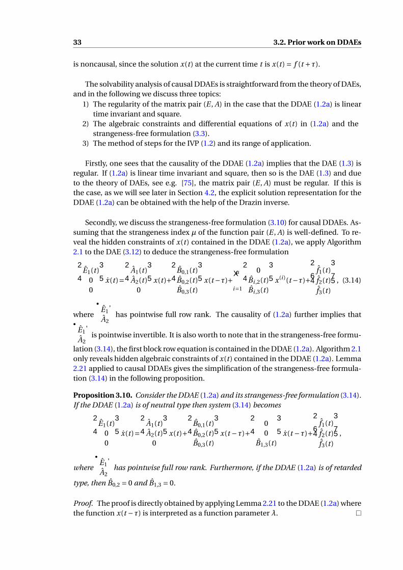
33 3.2. Prior work on DDAEs
is noncausal, since the solution x(t ) at the current time t is x(t ) = f (t +τ).
The solvability analysis of causal DDAEs is straightforward from the theory of DAEs,and in the following we discuss three topics:
1) The regularity of the matrix pair (E , A) in the case that the DDAE (1.2a) is lineartime invariant and square.
2) The algebraic constraints and differential equations of x(t ) in (1.2a) and thestrangeness-free formulation (3.3).
3) The method of steps for the IVP (1.2) and its range of application.
Firstly, one sees that the causality of the DDAE (1.2a) implies that the DAE (1.3) isregular. If (1.2a) is linear time invariant and square, then so is the DAE (1.3) and dueto the theory of DAEs, see e.g. [75], the matrix pair (E , A) must be regular. If this isthe case, as we will see later in Section 4.2, the explicit solution representation for theDDAE (1.2a) can be obtained with the help of the Drazin inverse.
Secondly, we discuss the strangeness-free formulation (3.10) for causal DDAEs. As-suming that the strangeness index µ of the function pair (E , A) is well-defined. To re-veal the hidden constraints of x(t ) contained in the DDAE (1.2a), we apply Algorithm2.1 to the DAE (3.12) to deduce the strangeness-free formulationE1(t )
00
x(t )=A1(t )
A2(t )0
x(t )+B0,1(t )
B0,2(t )B0,3(t )
x(t −τ)+µ∑
i=1
0Bi ,2(t )Bi ,3(t )
x(i )(t −τ)+
f1(t )f2(t )f3(t )
, (3.14)
where
[E1
A2
]has pointwise full row rank. The causality of (1.2a) further implies that[
E1
A2
]is pointwise invertible. It is also worth to note that in the strangeness-free formu-
lation (3.14), the first block row equation is contained in the DDAE (1.2a). Algorithm 2.1only reveals hidden algebraic constraints of x(t ) contained in the DDAE (1.2a). Lemma2.21 applied to causal DDAEs gives the simplification of the strangeness-free formula-tion (3.14) in the following proposition.
Proposition 3.10. Consider the DDAE (1.2a) and its strangeness-free formulation (3.14).If the DDAE (1.2a) is of neutral type then system (3.14) becomesE1(t )
00
x(t )=A1(t )
A2(t )0
x(t )+B0,1(t )
B0,2(t )B0,3(t )
x(t −τ)+ 0
0B1,3(t )
x(t −τ)+
f1(t )f2(t )f3(t )
,
where
[E1
A2
]has pointwise full row rank. Furthermore, if the DDAE (1.2a) is of retarded
type, then B0,2 = 0 and B1,3 = 0.
Proof. The proof is directly obtained by applying Lemma 2.21 to the DDAE (1.2a) wherethe function x(t −τ) is interpreted as a function parameter λ.

3.2. Prior work on DDAEs 34
Finally, we discuss the direct extension of the method of steps presented in Section2.5 to causal DDAEs. Introducing new sequences of matrix-valued and vector-valuedfunctions on the time interval [0,τ] as follows
Ei (t ) :=E(t + (i −1)τ), Ai (t ):=A(t + (i −1)τ), Bi (t ):=B(t + (i −1)τ),
fi (t ) := f (t + (i −1)τ), xi (t ):=x(t + (i −1)τ),(3.15)
for i ∈N and x0(t ) :=φ(t −τ). Thus, one can rewrite the IVP (1.2) as the set of DAEs
Ei (t )xi (t ) = Ai (t )xi (t )+Bi (t )xi−1(t )+ fi (t ), i = 1, 2, . . . ,`, (3.16a)
for all t ∈ (0,τ). Here, for each i , the equation (3.16a) is a DAE in variable xi , with afunction parameter xi−1.It is worth pointing out that for the DAE (3.16a), the initial condition xi (0) cannot bearbitrarily chosen as in the DDEs case, and usually the continuity of a solution at thepoint iτ, i.e.,
xi (0) = xi−1(τ), (3.16b)
leads to additional constraints that an initial functionφmust obey, as demonstrated inExample 3.11 below.
Example 3.11. Consider the following DDAE
0 · x(t ) = 1 · x(t )−1 ·x(t −τ), for all t ∈ [0,∞). (3.17)
Equation (3.16a) becomes 0 = xi (t )− xi−1(t ), for all t ∈ (0,τ). As a result, for i = 1 wehave x1(0) = x0(0) and hence, the condition (3.16b) yields φ(0) =φ(−τ).
In analogy to DDEs, for DDAEs the method of steps seeks for the solution xi of(3.16) provided that the function xi−1 is already known. Having found the functionsequence xi , i = 1, 2, . . . , the solution x(t ) of the IVP (1.2) is reconstructed step bystep via
x(t ) = xi (t − (i −1)τ), for every t ∈ [(i −1)τ, iτ]. (3.18)
Clearly, this strategy succeeds if and only if for every i , the IVP (3.16) has a unique solu-tion xi . This requirement implies that the method of steps is only applicable for causalDDAEs.
In previous work, the method of steps has only been considered for retarded orneutral DDAEs, see e.g. [31, 83, 122, 131, 142] for the application to linear systemsand [5, 60, 68, 86, 143] for the application to nonlinear systems. This is quite reason-able since until now, a numerical solution procedure for general advanced DDEs, thespecial case of advanced DDAEs, is not available. The interesting property that hasnot been mentioned in previous studies about DDAEs is that in some special cases,numerical integration for advanced DDAEs is still feasible, as shown in the followingexample.

35 3.3. Characteristics of general linear DDAEs
Example 3.12. Consider the DDAE[0 10 0
][x1(t )x2(t )
]=[
1 00 1
][x1(t )x2(t )
]+[
1 00 1
][x1(t −τ)x2(t −τ)
]+[
1−e t −e t−1
1−2t
], (3.19)
in the time interval I = [0,∞), with the delay τ = 1 and an initial function φ(t ) =[
e t
t
]for t ∈ [−τ,0]. Differentiating the second equation to obtain x2 and inserting it into thefirst equation to eliminate x2, one obtains the strangeness-free DDAE[
0 00 0
][x1(t )x2(t )
]=[
1 00 1
][x1(t )x2(t )
]+[
1 00 1
][x1(t −τ)x2(t −τ)
]+[
0 10 0
][x1(t −τ)x2(t −τ)
]+[−1−e t −e t−1
1−2t
],
(3.20)which implies that (3.19) is of advanced type. As noted in Section 2.5, in general, ifthe time interval is [0,∞) then an initial function φ must be infinitely differentiableto guarantee the existence of a solution x ∈ C (I,Cn). However, from (3.20), we see thatthe smoothness requirement for φ is φ ∈ C 1([−τ,0],Cn). As a result, for the numericalsolution, we only need to care about the discontinuities of φ, φ but not of the higherderivatives of φ. The numerical solution of the corresponding IVP for (3.19) is success-fully computed by using the method of steps. The numerical solution and the absolute
error with respect to the exact solution x(t ) =[
e t
t
]are presented in Figure 3.1. The sim-
ulation is done by using the three stage Radau IIA method of [60] with constant step sizeh = 0.1 for the strangeness-free DDAE (3.20) on the simulation time interval [0,10τ].
0 2 4 6 8 1010−2
100
102
104
106
x1x2
0 2 4 6 8 1010−20
10−15
10−10
10−5
100
error x1error x2
Figure 3.1: Numerical solution and absolute error of the IVP (1.2) for (3.19) with constantstepsize h = 0.1.
3.3 Characteristics of general linear DDAEs
Evidently, DDAEs inherit properties from their subclasses, for example, from the DAEside the structure of the matrix function pair (E , A), and from the DDE side the infinitedimensional solution space. However, the combination of these two subclasses has in-troduced many new features to (1.2a), which occur neither for DAEs nor for DDEs, seee.g. [25, 31, 63, 65]. As we have seen in Section 3.2, the noncausality of DDAEs plays a

3.3. Characteristics of general linear DDAEs 36
very important role in the solvability analysis, and therefore we discuss in this sectionsome characteristics of general noncausal DDAEs, which are starting points for impor-tant consequences on the numerical integration of the IVP (1.2).
Firstly, unlike causal DDAEs, the solvability of noncausal DDAEs involves the struc-ture of three matrix-functions E , A, B instead of only two matrix functions E , A. In par-ticular, for linear time invariant DDAEs, it is not necessary that the matrix pair (E , A)must be regular to obtain the regularity of the DDAE (1.2a). Revisit the DDAE (3.13),we see that even though the matrix pair (E , A) = (0,0) is not regular, (3.13) still has aunique solution x(t ) = f (t +τ).
Secondly, since DDAEs are in general noncausal, some constraints of a present state(x(t )) may be hidden in the equations at future times such as t +τ, t +2τ, . . . . Thus, inorder to determine a present state, one may have to utilize the equation at multiplefuture time points. This can be easily seen from the following example.
Example 3.13. Consider the DDAE[1 00 0
]x(t ) =
[0 00 0
]x(t )+
[0 00 1
]x(t −τ)+
[1−t
], (3.21)
for all t ∈ (0,∞). An initial function x(t ) = φ(t ) for t ∈ [−τ,0]. Consider any fixedt ∈ (0,τ) and insert x(t − τ) = φ(t − τ) into (3.21) yields an underdetermined system,which does not uniquely determine the second component of x(t ). Nevertheless, theDDAE (3.21) at the future point t +τ gives rise to the system[
1 00 0
]x(t +τ) =
[0 00 1
]x(t )+
[1
−t −τ]
, (3.22)
which contains the algebraic constraint 0 = [0 1]
x(t )−t−τ. The coupled system (3.21)-(3.22) uniquely determines x(t ), which means that one needs to utilize (3.21) at least attwo time points t and t +τ to determine x(t ).
This noncausal characteristic also implies that for DDAEs, in order to determinethe present state x(t ), one can use at least two different operators:i) The shift (forward) operator ∆−τ that maps the equation (1.2a) into the equation
E(t +τ)x(t +τ) = A(t +τ)x(t +τ)+B(t +τ)x(t )+ f (t +τ),
provided that the point t satisfies t < t f −τ.ii) The differentiation operator that maps the equation (1.2a) into the equation
d
dt(E(t )x(t )− A(t )x(t )) = d
dt
(B(t )x(t −τ)+ f (t )
), (3.23)
For the determination of x(t ) at an arbitrary point t , the differentiation operator isuseless, since the DDAE (3.23) is only a consequence of the DDAE (1.2a). On the otherhand, the shift operator presents a critical restriction to the solution space of the DDAEs(1.2a). We illustrate this fact by revisiting the DDAE (3.13) at one point t ∈ I. Let

37 3.3. Characteristics of general linear DDAEs
g (t ) := x(t −τ)− t . Applying the differentiation operator to (3.13) leads to the system
0 · x(t ) = 0 ·x(t )+ g (t ),
0 · x(t ) = 0 · x(t )+ g (t ),
which is still not enough to uniquely determine x(t ). On the other hand, applying theshift operator to (3.13) leads to the system
0 · x(t ) = 0 · x(t )+ g (t ),
0 · x(t +τ) = 0 · x(t +τ)+x(t )− (t +τ),
that uniquely determines x(t ). Since the shift operator is influenced by the time inter-val I, it follows that the solvability analysis of the IVP (1.2) also depends on the timeinterval I.
Remark 3.14. It is also important to note that in general the two operatorsd
dtand
∆−τ do not commute, since the derivatives of the functions E , A, B , x, f may existat the point t + τ but do not exist at the point t , or vice versa. Finding an optimalway to combine the differentiation and shift operators, in order to fully understand thesolvability of the DDAE (1.2a) and to compute the solution of the IVP (1.2) is still anopen problem, see [63, 65] for some partial results.
Now let us consider the constraints of x(t ) contained in the DDAE (1.2a) and thestrangeness-free formulation of (1.2a). For causal DDAEs, we already know that:
1) There may exist hidden algebraic constraints but no hidden differential equa-tions of x(t ) in (1.2a).
2) An underlying DDE of a causal DDAE is a first order DDE.However, for noncausal DDAEs, these properties no longer hold, as demonstrated be-low.
Example 3.15. Considering again the DDAE (3.6), we see that it has a hidden differentialequation
0 = x1(t )−e t .
Furthermore, from the strangeness-free formulation (3.9) of the DDAE (3.6), by differ-entiating the first two equations twice, we deduce an implicitly formulated underlyingDDE
−0 1 0
0 0 11 0 0
x1(t )x2(t )x3(t )
=0 0 0
1 0 00 0 0
x1(t −1)x2(t −1)x3(t −1)
+1 0 0
0 0 00 0 0
x(3)
1 (t −1)x(3)
2 (t −1)x(3)
3 (t −1)
+−e t−1
−e t−1
−e t
,
which is of second order.
In general, if the DDAE (1.2a) is noncausal and of advanced type then the strangeness-free formulation and the underlying DDE can be of arbitrarily high orders in both x(t )and x(t −τ). If this is the case, applying numerical methods like Runge-Kutta or BDFmethods to the strangeness-free formulation will be complicated and may not be fea-sible.
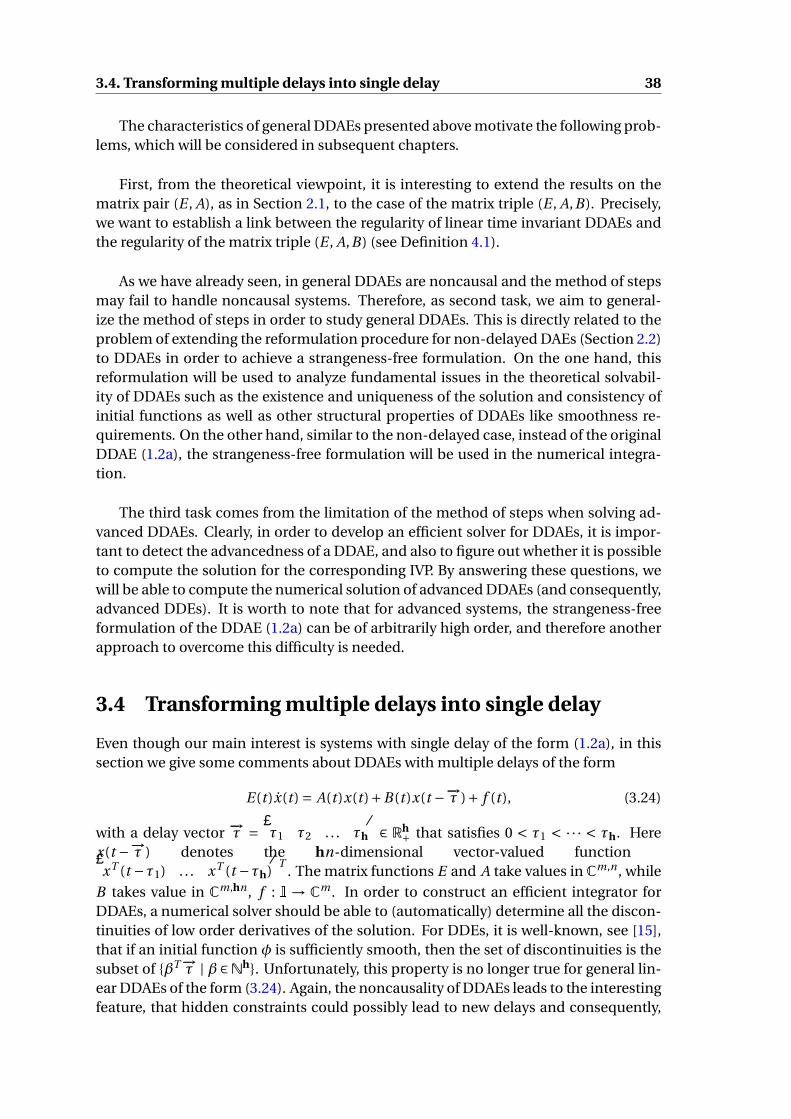
3.4. Transforming multiple delays into single delay 38
The characteristics of general DDAEs presented above motivate the following prob-lems, which will be considered in subsequent chapters.
First, from the theoretical viewpoint, it is interesting to extend the results on thematrix pair (E , A), as in Section 2.1, to the case of the matrix triple (E , A,B). Precisely,we want to establish a link between the regularity of linear time invariant DDAEs andthe regularity of the matrix triple (E , A,B) (see Definition 4.1).
As we have already seen, in general DDAEs are noncausal and the method of stepsmay fail to handle noncausal systems. Therefore, as second task, we aim to general-ize the method of steps in order to study general DDAEs. This is directly related to theproblem of extending the reformulation procedure for non-delayed DAEs (Section 2.2)to DDAEs in order to achieve a strangeness-free formulation. On the one hand, thisreformulation will be used to analyze fundamental issues in the theoretical solvabil-ity of DDAEs such as the existence and uniqueness of the solution and consistency ofinitial functions as well as other structural properties of DDAEs like smoothness re-quirements. On the other hand, similar to the non-delayed case, instead of the originalDDAE (1.2a), the strangeness-free formulation will be used in the numerical integra-tion.
The third task comes from the limitation of the method of steps when solving ad-vanced DDAEs. Clearly, in order to develop an efficient solver for DDAEs, it is impor-tant to detect the advancedness of a DDAE, and also to figure out whether it is possibleto compute the solution for the corresponding IVP. By answering these questions, wewill be able to compute the numerical solution of advanced DDAEs (and consequently,advanced DDEs). It is worth to note that for advanced systems, the strangeness-freeformulation of the DDAE (1.2a) can be of arbitrarily high order, and therefore anotherapproach to overcome this difficulty is needed.
3.4 Transforming multiple delays into single delay
Even though our main interest is systems with single delay of the form (1.2a), in thissection we give some comments about DDAEs with multiple delays of the form
E(t )x(t ) = A(t )x(t )+B(t )x(t −−→τ )+ f (t ), (3.24)
with a delay vector −→τ = [τ1 τ2 . . . τh] ∈ Rh+ that satisfies 0 < τ1 < ·· · < τh. Here
x(t −−→τ ) denotes the hn-dimensional vector-valued function[xT (t −τ1) . . . xT (t −τh)
]T. The matrix functions E and A take values in Cm,n , while
B takes value in Cm,hn , f : I → Cm . In order to construct an efficient integrator forDDAEs, a numerical solver should be able to (automatically) determine all the discon-tinuities of low order derivatives of the solution. For DDEs, it is well-known, see [15],that if an initial function φ is sufficiently smooth, then the set of discontinuities is thesubset of βT−→τ | β ∈Nh. Unfortunately, this property is no longer true for general lin-ear DDAEs of the form (3.24). Again, the noncausality of DDAEs leads to the interestingfeature, that hidden constraints could possibly lead to new delays and consequently,

39 3.4. Transforming multiple delays into single delay
increase the set of discontinuities of low order derivatives of x.
Example 3.16. Consider the DDAE[1 00 0
]x(t ) =
[0 01 0
]x(t )+
[0 00 1
]x(t −1)+
[0 01 1
]x(t −π), (3.25)
on the time interval I = [0,∞). Formally, two delays 1 and π are explicitly present in(3.25). However, a new delay also arises as we will see below. To deduce the hidden con-straint of (3.25), we subtract the derivative of the second equation from the first equationto obtain [
0 0]
x(t ) = [0 0]
x(t )+ [0 1]
x(t −1)+ [1 1]
x(t −π).
Shifting this equation forward by 1, we get
0 = [0 1]
x(t )+ [1 1]
x(t −π+1),
which implies that π−1 is also a delay of (3.25).
To figure out how many new delays can arise in the DDAE (1.2a), one has to de-velop a systematic theory for the regularization of DDAEs with multiple delays. At themoment, this question is still open. Nevertheless, in the case of commensurate delays,one can transform a multiple delay system into a new one with only one single delay.We now present this technique for DDAEs.
Let us consider the DDAEs (3.24) with commensurate delays, i.e. the delay vector −→τsatisfies τi /τ j ∈ Q for all i , j . In order to generate the transformation such that thenumber of state variables of the transformed system is minimal, we look for the max-imal value of the constant τ0 such that τi /τ0 ∈ N for all i = 1, . . . ,h. This τ0 can beobtained from the following lemma.
Lemma 3.17. Let τi /τ1 = ai /bi for i = 2, . . . ,h, with ai , bi ∈ N and g cd(ai ,bi ) = 1.Then, the maximal value of the delay constant τ0 such that τi /τ0 ∈N for all i = 1, . . . ,his given by τ0 = τ1/lcm(b2, . . . ,bh).
Proof. For the proof see e.g. [120], Lemma 2.1.
Let ci = τi /τ0 ∈ N and partitioning B as[B1 . . . Bh
]where Bi : I→ Cm,n , for 1, . . . ,h,
we can rewrite the DDAE (3.24) as
E(t )x(t ) = A(t )x(t )+h∑
i=1Bi (t )x(t − ciτ0)+ f (t ). (3.26)
Introducing h := ch and adapting the matrices Bi accordingly, we can rewrite (3.26) as
E(t )x(t ) = A(t )x(t )+h∑
i=1Bi (t )x(t − iτ0)+ f (t ). (3.27)
Then, the DDAE (3.27) can be rewritten as
E new (t )X new (t ) = Anew (t )X new (t )+B new (t )X new (t −τ0)+ f new (t ), (3.28)

3.4. Transforming multiple delays into single delay 40
with coefficients and variables given by
E new :=
E
0. . .
00
, Anew :=
A B1 . . . Bh−2 Bh−1
I. . .
II
,
B new :=
0 0 . . . 0 Bh−I 0
. . . . . .. . . 0
−I 0
, f new :=
f (t )
0...00
, X new (t ):=
x(t )
x(t −τ0)...
x(t − (h−2)τ0)x(t − (h−1)τ0)
.
Using this transformation, fundamental properties such as solvability, stability andcontrollability criteria derived for single delay systems can at once be extended to mul-tiple delay systems. In particular, one can make use of all the results in subsequentchapters of this work to analyze the solvability of the multiple delay DDAE (3.24). Fi-nally, it is worth to note that for the study of numerical solutions to DDAEs, this strategyonly makes sense if the delay τ0 of the DDAE (3.28) is not too small, compared to τh.Otherwise, the size of the DDAE (3.28) can be very high.

Chapter 4
Solvability Analysis of General LinearTime Invariant DDAEs
This chapter is devoted to a special case of the DDAE (1.2a), where all the functioncoefficients E , A, B are constant matrices. Thus, the IVP (1.2) becomes
E x(t ) = Ax(t )+B x(t −τ)+ f (t ), (4.1a)
x|[−τ,0] =φ. (4.1b)
Inspired by the application of matrix pencils to the solvability analysis of DAEs, wewish to extend the results of Section 2.1 to the case of the matrix triple (E , A,B). Pre-cisely, we want to establish a link between the regularity of the matrix triple (E , A,B)(see Definition 4.1) and the regularity of the DDAE (4.1a). As shown in Section 3.3, theboundedness of the time interval I plays an important role in the solvability analysisof DDAEs. Thus, this chapter is roughly divided into two cases: bounded time interval(Section 4.2) and unbounded time interval (Section 4.3).
4.1 Basic properties
Within this section, we present some basic properties of linear time invariant DDAEs.In the following definition, we extend the concept of regularity from matrix pairs tomatrix triples.
Definition 4.1. Consider the DDAE (4.1a). The matrix triple (E , A,B) ∈ (Cm,n)3 is calledregular if m = n and the so-called characteristic exponential polynomial p(λ) definedby
p(λ) = det(λE − A−e−λτB)
is not identically zero.
Clearly, the triple (E , A,B) is regular if and only if the spectrum
σ(E , A,B) := λ ∈C | det(λE − A−e−λτB) = 0,
is not the entire C. Elements of the spectrum σ(E , A,B) are called eigenvalues of the
41

4.1. Basic properties 42
triple (E , A,B). Note that it does not make sense to talk about infinite eigenvalues, be-cause the limit of p(λ) does not exist when |λ|→∞. This is in contrast to the non-delaycase. The next proposition shows that, similar to DAEs, the spectrum of the matrixtriple (E , A,B) is important in the understanding of DDAEs. In comparison with DAEs,see Theorem 2.8.
Proposition 4.2. Consider the DDAE (4.1a) on the time interval I. If rank(λE − A −e−λτB) < n for all λ ∈C then the homogeneous IVP
E x(t ) = Ax(t )+B x(t −τ), x|[−τ,0] = 0, (4.2)
has a nontrivial solution.
Proof. To prove the claim, let us take n+1 different complex numbers λ1, . . . ,λn+1. Foreach i , since rank(λi E − A − e−λiτB) < n, there exists a vector vi ∈ Cn \ 0 that fulfills(λi E − A − e−λiτB)vi = 0. The linear dependence of n + 1 vectors vi , i = 1, . . . ,n + 1implies that there exist numbersαi , i = 1, . . . ,n+1, not all of them being zero, such that
n+1∑i=1
αi vi = 0.
Let the function x : [−τ, t f ) →Cn be defined by
x(t ) =
0, −τ6 t 6 0,∑n+1i=1 αi eλi t vi , t > 0,
we see that x(t ) is continuous at t = 0 and x(t ) satisfies the equation (4.2) for t > 0.Thus x is a nontrivial solution of the homogeneous IVP (4.2).
Recall from Theorem 2.8 that if rank(λE − A) = n < m for some λ ∈ C, then thereexists an arbitrarily smooth function f such that the DAE E x(t ) = Ax(t )+ f (t ) is notsolvable. For DDAEs, we demonstrate in the following two examples that this propertydepends on the time interval I.
Example 4.3. Consider the DDAE[10
]x(t ) =
[00
]x(t )+
[01
]x(t −τ)+
[f1(t )f2(t )
], (4.3)
on the time interval I= [0,τ). Obviously, (λE − A) has full column rank for λ= 1.
If the delay term
[01
]x(t−τ) does not appear, then the second equation 0 = f2(t ) certainly
gives us a consistency condition that f must obey. Therefore, by choosing a smooth func-tion f such that f2 6≡ 0, the non-delayed DAE[
10
]x(t ) =
[00
]x(t )+
[f1(t )f2(t )
],
has no solution.
However, if the delay term
[01
]x(t−τ) is present then the second equation is 0 = x(t−τ)+

43 4.2. Systems on bounded time intervals
f2(t ) for all t ∈ I= [0,τ]. In contrast to the DAE case, this is not a consistency conditionfor f , but a consistency condition for an initial function φ. More precisely, 0 = φ(t −τ)+ f2(t ), for all t ∈ [0,τ]. Thus, for any continuous function f , there exists a consistentinitial function φ such that the corresponding IVP (1.2) for the DDAE (4.3) is solvable.
Example 4.4. Now we consider again the DDAE (4.3), but on the time interval I= [0,∞).The second equation implies that
0 = x(t −τ)+ f2(t ),
for all t ∈ [0,∞). Shifting this equation forward by τ, one has 0 = x(t )+ f2(t +τ). Ob-serving from the first equation of (4.3) that x(t ) = f1(t ), one obtains f1(t ) = − f2(t +τ),which is a consistency condition for f . By choosing any smooth function f that violatesthis condition, the IVP (1.2) for (4.3) is not solvable.
In the next two sections, we will examine DDAEs more carefully in two cases ofbounded and unbounded time intervals.
4.2 Systems on bounded time intervals
In this section we will particularly deal with DDAEs on a bounded time interval. Themethod of steps applied to the DDAE (4.1a) yields the following equations
E xi (t ) = Axi (t )+B xi−1(t )+ fi (t ), i = 1, 2, . . . ,`, (4.4)
for all t ∈ (0,τ). We recall that the functions xi , i ∈N are defined by xi (t ) := x(t+(i−1)τ)and x0(t ) :=φ(t −τ).
The following lemma gives a necessary condition for the existence and uniquenessof the solution x for the IVP (4.1).
Lemma 4.5. Consider the IVP (4.1) on the bounded time interval I. Assume that theDDAE (4.1a) is square, i.e., m = n. Then, the DDAE (4.1a) is regular only if the matrixpair (E , A) is regular.
Proof. Assume that the DDAE (4.1a) is regular. This implies that the restriction of theIVP (4.1) on the last interval [(`− 1)τ,`τ] has a unique solution. From the theory ofDAEs [75], we see that the square DAE
E x`(t ) = Ax`(t )+ g`(t ),
where g`(t ) := B x`−1(t )+ f`(t ), has a unique solution only if the matrix pair (E , A) isregular.
Assuming the regularity of the matrix pair (E , A), we can now use the theory of DAEsto study equation (4.1a). We will go along the lines of [25, 26] to obtain the explicitsolution of the IVP (4.1) and then to derive the necessary conditions for a consistentinitial function φ. Let λ0 be an arbitrary real number such that the inverse of λ0E − A

4.2. Systems on bounded time intervals 44
exists and set
E = (λ0E − A)−1E , A = (λ0E − A)−1 A, B = (λ0E − A)−1B , fi = (λ0E − A)−1 fi ,
P = E D E , Q = E D A, H = E AD .
Then P is a projection, i.e., P 2 = P , E and A commute, P , Q and H pairwise commute.Let ν be the Kronecker-index of the matrix pair (E , A), the explicit representation of thesolution xi to (4.4) is established due to Theorem 2.7 as
xi (t )=P
[eQt xi (0)+
∫ t
0eQ(t−s) (B xi−1(s)+ fi (s)
)d s
]−(I −P )
ν−1∑j=0
H j AD(B x( j )
i−1(t )+ f ( j )i (t )
),
(4.5)for all t ∈ [0,τ] and i ∈N.Now let us consider the influence of the condition xi (0) = xi−1(τ) on an initial functionφ. From (4.5) we find that
xi (0)−xi−1(τ) = P
[xi (0)−eQτxi−1(0)−
∫ τ
0eQ(τ−s) (B xi−2(s)+ fi−1(s)
)d s
]−(I −P )
ν−1∑j=0
H j AD[
B(x( j )
i−1(0)−x( j )i−2(τ)
)+(
f ( j )i (0)− f ( j )
i−1(τ))]
.
Let us further assume that f ∈Cν−1([0,∞),Cn), then f ( j )i (0) = f ( j )
i−1(τ) and hence,
xi (0)−xi−1(τ) = P
[xi (0)−eQτxi−1(0)−
∫ τ
0eQ(τ−s) (B xi−2(s)+ fi−1(s)
)d s
]−(I −P )
ν−1∑j=0
H j AD B(x( j )
i−1(0)−x( j )i−2(τ)
).
Note that the condition xi (0) = xi−1(τ) is equivalent to the coupled system of equations
P xi (0) = P xi−1(τ), (4.6a)
(I −P )xi (0) = (I −P )xi−1(τ). (4.6b)
Regardless of what xi−1(τ) is, choosing P xi (0) = P xi−1(τ) makes the part P x(t ) of thesolution x(t ) of the DDAE (4.1) continuous at the point (i −1)τ. Precisely, we choose
P xi (0) = P
[eQτxi−1(0)+
∫ τ
0eQ(τ−s) (B xi−2(s)+ fi−1(s)
)d s
]. (4.7)
On the other hand,
(I −P )xi (0)− (I −P )xi−1(τ) = (I −P )ν−1∑j=0
H j AD B(x( j )
i−1(0)−x( j )i−2(τ)
). (4.8)
Thus, condition (4.6b) holds if x( j )i−1(0) = x( j )
i−2(τ) for all j = 0, . . . ,ν−1. Furthermore, thehigh derivatives of xi are given by the following lemma.
Lemma 4.6. Consider the formula (4.5). Assume that the functions xi−1 and fi are suf-

45 4.2. Systems on bounded time intervals
ficiently smooth. Then for every α ∈N, we have
x(α)i (t ) = PeQtQαxi (0)+PeQtQα
∫ t
0e−Qs (B xi−1(s)+ fi (s)
)d s
+α−1∑j=0
(α
j +1
)PQα− j−1
(B x( j )
i−1(t )+ f ( j )i (t )
)−(I−P )
ν−1∑j=0
H j AD(B x( j+α)
i−1 (t )+ f ( j+α)i (t )
).
(4.9)
Proof. From (4.5), one sees that for any α ∈N,
x(α)i (t ) = PeQtQαxi (0)+PeQtQα
∫ t
0e−Qs (B xi−1(s)+ fi (s)
)d s
+α∑
j=1
(α
j
)PQα− j
(B xi−1(t )+ fi (t )
)( j−1)−(I−P )ν−1∑j=0
H j AD(B x( j+α)
i−1 (t )+ f ( j+α)i (t )
),
which implies the desired form (4.9).
Using Lemma 4.6, we can further analyze the continuity of arbitrarily high orderderivatives of the solution x(t ) at the points (i −1)τ as follows.
Lemma 4.7. Consider the IVP (4.1) and system (4.4). Assume that the function f of theDDAE (4.1) and the functions xi−1, xi−2 are sufficiently smooth. Letα ∈N and P xi (0) be
given by (4.7). If x( j )i−1(0) = x( j )
i−2(τ) for all j = 1, . . . ,ν−1+α, then x(α)i (0) = x(α)
i−1(τ).
Proof. If suffices to prove that (I −P )(x(α)
i (0)−x(α)i−1(τ)
)= 0 and P
(x(α)
i (0)−x(α)i−1(τ)
)= 0.
From (4.9), it follows that
(I −P )(x(α)
i (0)−x(α)i−1(τ)
)=−(I−P )
ν−1∑j=0
H j AD(B(x( j+α)
i−1 (0)−x( j+α)i−2 (τ)
)+ f ( j+α)
i (0)− f ( j+α)i−1 (τ)
)=−(I−P )
ν−1∑j=0
H j AD(
f ( j+α)i (0)− f ( j+α)
i−1 (τ))
,
and due to the continuity of f ( j+α) at (i −1)τ, we see that (I −P )(x(α)
i (0)−x(α)i−1(τ)
)= 0.
On the other hand, from (4.9) we see that
P x(α)i (0) = PQαxi (0)+
α−1∑j=0
(α
j +1
)PQα− j−1
(B x( j )
i−1(0)+ f ( j )i (0)
),
= PQαxi (0)+α−1∑j=0
(α
j +1
)PQα− j−1
(B x( j )
i−2(τ)+ f ( j )i−1(τ)
),

4.2. Systems on bounded time intervals 46
and due to (4.7) and the commutativity of P and Q, it follows that
P x(α)i (0) = PQα
[eQτxi−1(0)+
∫ τ
0eQ(τ−s) (B xi−2(s)+ fi−1(s)
)d s
]+α−1∑j=0
(α
j +1
)PQα− j−1
(B x( j )
i−2(τ)+ f ( j )i−1(τ)
).
(4.10)
By direct computation, using (4.9), we see that P x(α)i−1(τ) is exactly the right hand side
of (4.10). Therefore, P(x(α)
i (0)−x(α)i−1(τ)
)= 0 and hence, we obtain x(α)
i (0) = x(α)i−1(τ).
Summarizing the arguments above, one obtains the following lemma.
Lemma 4.8. Consider the IVP (4.1) and system (4.4). Assume that f is sufficiently smooth.For any 16 i 6 `, let the part P xi (0) be chosen as in (4.7). Then the following assertionshold.i) If x( j )
i−1(0) = x( j )i−2(τ) for all j = 0, . . . ,ν−1 then xi (0) = xi−1(τ).
ii) If x( j )1 (0) = x( j )
0 (τ) for all j = 0, . . . , i (ν−1) then xi (0) = xi−1(τ).
Proof. We prove the first claim by checking the coupled system (4.6). With P xi (0) cho-sen as in (4.7), one obtains (4.6a). On the other hand, it is clear that (4.6b) holds due to(4.8). The second claim is a direct consequence of Lemma 4.7 by induction.
In the following theorem we characterize the solvability analysis of linear time in-variant DDAEs on a bounded time interval.
Theorem 4.9. Consider the square DDAE (4.1a) on the bounded time interval I= [0,`τ).Furthermore, assume that the inhomogeneity f is sufficiently smooth. Then the DDAE(4.1a) is regular only if the matrix pair (E , A) is regular. If this is the case, let ν be theKronecker-index of the matrix pair (E , A). A sufficient condition for the existence anduniqueness of the solution x is that the following conditions hold:i) The initial function φ satisfies φ ∈C`(ν−1)+1([−τ,0],Cn).ii) The following identities are satisfied
φ(α)(0−) = PQαφ(0)+α−1∑j=0
(α
j +1
)PQα− j−1
(Bφ( j )(−τ+)+ f ( j )
1 (0))
− (I −P )ν−1∑j=0
H j AD(Bφ( j+α)(−τ+)+ f ( j+α)
1 (0)),
(4.11)
for α= 0, . . . ,`(ν−1).
Proof. The first claim is exactly Lemma 4.5. For the second claim, one needs to analyzewhether the function x(t ) given by (4.5) is a solution of the IVP (4.1). Substituting i = 1and t = 0 into (4.9), one has
x(α)1 (0) = PQαx1(0)+
α−1∑j=0
(α
j +1
)PQα− j−1
(B x( j )
0 (0)+ f ( j )1 (0)
)− (I −P )
ν−1∑j=0
H j AD(B x( j+α)
0 (0)+ f ( j+α)1 (0)
).
(4.12)

47 4.3. Systems on unbounded time intervals
From (4.11) and (4.12), one sees that x(α)1 (0) = φ(α)(0−) and hence, x(α)
1 (0) = x(α)0 (τ) for
allα= 0, . . . ,`(ν−1). Lemma 4.8 therefore implies the continuity of the solution x at thepoints iτ, 06 i 6 `, and hence the IVP (4.1) has a unique solution given by (4.5).
Remark 4.10. The conditions i)-ii) in Theorem 4.9 are only sufficient but not necessaryto ensure the existence and uniqueness of a solution to the IVP (4.1). The reason is thatin some cases, the actual smoothness requirement for φ is more relaxed than i). This isillustrated in the following example.
Example 4.11. Consider the IVP consisting of the DDAE[0 10 0
][x(t )y(t )
]=[
1 00 1
][x(t )y(t )
]−[
1 00 1
][x(t −τ)y(t −τ)
]+[
f1(t )f2(t )
], (4.13)
for t ∈ I= [0,`τ), with an initial function φ(t ) :=[φ1(t )φ2(t )
], for t ∈ [−τ,0].
Applying Theorem 4.9 to (4.13), one sees that ν= 2 and the smoothness requirement forφ is that φ ∈C`+1([−τ,0],C2). Nevertheless, one can derive from (4.13) that
x(t ) = x(t −τ)+ y(t −τ)− f1(t )− f2(t ),
y(t ) = y(t −τ)− f2(t ),
and therefore, the necessary and sufficient smoothness requirement for an initial func-tion is only φ1 ∈C ([−τ,0],C) and φ2 ∈C 1([−τ,0],C).
Remark 4.12. It is worth to note that the results presented in this section are based onthe regularity of the matrix pair (E , A). Under this condition, even if the time interval Iis unbounded, all the results in this section are still valid.
4.3 Systems on unbounded time intervals
Now we consider the DDAE (4.1a) on the unbounded time interval I= [0,∞). Unfortu-nately, the regularity of the DDAE (4.1a) no longer implies the regularity of the matrixpair (E , A). A simple example is the equation
0 · x(t ) = 0 · x(t )+x(t −τ)− t ,
which has a unique solution x(t ) = t +τ, even though the matrix pair (E , A) = (0,0) issingular. Failing at deducing the regularity of the matrix pair (E , A), it is not possible towrite down the solution formula and discuss the solvability properties as it was done inSection 4.2. Thus, we need to extend the regularity concept to the matrix triple (E , A,B).
4.3.1 Structures of matrix triples via constant equivalence transfor-mations
Similar to the case of DAEs, one can transform the DDAE (4.1a) by employing constantequivalent transformations defined as follows.

4.3. Systems on unbounded time intervals 48
Definition 4.13. Two triples of matrices (E1, A1,B1) and (E2, A2,B2) in (Cm,n)3 are calledequivalent if there exist nonsingular matrices P ∈Cm,m and Q ∈Cn,n such that
(E2, A2,B2) = (PE1Q,PA1Q,PB1Q).
If this is the case, we write (E1, A1,B1) ∼ (E2, A2,B2).
This approach, however, has achieved only few results in special cases of the matrixtriple (E , A,B), see e.g. [30, 31]. Within this subsection, we first recall these resultsand then we consider another special case, where the matrix coefficients of (4.1) arepairwise commutative. In this subsection, we again assume that the DDAE (4.1a) issquare.
Lemma 4.14. Assume that the matrix triple (E , A,B) ∈ (Cn,n)3 is regular. Then,
(E , A,B) ∼N1 E12 E13
0 E22 E23
0 0 N2
,
N3 A12 A13
0 A22 A23
0 0 N4
,
I 0 00 B22 00 0 I
, (4.14)
where Ni , i = 1, . . . ,4, are strictly upper triangular matrices, and E22 and A22 are suchthat
(range(E22)+ range(A22)
)⊥ and kernel(E22)∩kernel(A22) are both 0. Further-more, it is allowed that any of the block rows (and hence, the corresponding block col-umn) may not be present in (4.14).
Proof. See [30], Theorem 2.
Let us assume that E , A, B are already in the form (4.14). Partitioning the variable xand an inhomogeneity f correspondingly, we can rewrite the DDAE (4.1a) as
N1x1(t )=N3x1(t )+x1(t −τ)−E12x2(t )−E13x3(t )+A12x2(t )+A13x3(t )+ f1(t ), (4.15a)
E22x2(t )=A22x2(t )+B22x2(t −τ)+ (−E23x3(t )+ A23x3(t )+ f2(t ))
, (4.15b)
N2x3(t )=N4x3(t )+x3(t −τ)+ f3(t ). (4.15c)
First one sees that the function x3 is uniquely determined by equation (4.15c). The nextlemma gives us the explicit solution formula.
Lemma 4.15. Consider the equation (4.15c). Furthermore, suppose that f3 is sufficientlysmooth. Then (4.15c) has the unique solution
x3(t ) =−n−1∑i=0
(d
dtN2 −N4
)if3(t + (i +1)τ), (4.16)
for all t ∈ [−τ,∞).
Proof. Set L := ddt N2−N4 to be the linear operator, which maps a (continuously differ-
entiable) function x3 to N2x3−N4x3. Since N2, N4 are strictly upper triangular matricesof dimension at most n, we can directly verify that L n = 0.Consider the shift forward operator ∆−τ : x3(t ) 7→ x3(t +τ), which commutes with N2,

49 4.3. Systems on unbounded time intervals
N4, ddt , and hence, it commutes with L . Thus, equation (4.15c) in the operator form
becomesd
dtN2∆−τx3(t −τ)−N4∆−τx3(t −τ) = x3(t −τ)+ f3(t ),
or equivalently, one has (I −L∆−τ) x3(t −τ) =− f3(t ) for all t ≥ 0.This leads us to the solution formula
x3(t ) =− (I −L∆−τ)−1 f3(t +τ) =−n−1∑i=0
L i∆i−τ f3(t +τ),
for all t ≥−τ, that is exactly (4.16).
In the same way, one can uniquely determine x1 from (4.15a), provided that x2 isalready known. Thus, we are lead to the question whether x2 is uniquely determinedfrom (4.15b). The answer will be positive if the regularity of the matrix pair (E22, A22) isguaranteed and then we obtain the following proposition.
Proposition 4.16. Let the matrix triple (E , A,B) associated with the DDAE (4.1a) beregular and be given in the form (4.14). Furthermore, suppose that the matrix pair(E22, A22) as in (4.14) is also regular. Then, the decomposition (4.14) completely describesthe dynamics of the DDAE (4.1a).
Proof. See [30], Theorem 2.
Remark 4.17. Unfortunately, the regularity of the matrix pair (E22, A22) is only a suffi-cient condition for the existence and uniqueness of a solution x to the DDAE (4.1a), asshown in Example 4.18 below.
Example 4.18. [30] Consider the DDAE (4.1a) with the matrix coefficients
E =1 0 0
0 0 10 0 0
, A =0 1 0
0 0 00 0 1
, B =0 0 1
1 0 00 1 0
.
The inhomogeneity f is chosen so that one obtains any desired solution. One can seethat the form (4.14) for such matrices E, A, B has only one non-empty block row and onenon-empty block column E22 = E, A22 = A, B22 = B. Clearly, the matrix pair (E22, A22) issingular. However, the DDAE (4.1a) still has a unique solution.
Another attempt to explore the structure of matrix triple (E , A,B) can be made inthe case that these three matrices are pairwise commutative.
Definition 4.19. Let E , A, B ∈ Cn,n . The matrix triple (E , A,B) is called a commutativetriple if E , A, and B pairwise commute.
Definition 4.20. i) Let R = [ri j ] ∈Cm,n and S ∈Cp,q . The mp by nq matrix R⊗S = [ri j S]is called the Kronecker product of R and S.ii) The vec operator creates a column vector from a matrix R = [r1 r2 . . . rn
] ∈Cm,n

4.3. Systems on unbounded time intervals 50
by stacking the column vectors of R below one another:
vec(R) =
r1
r2...
rn
.
Theorem 4.21. Let R ∈Cm,n , W ∈Cn,p and S ∈Cp,q . Then,
vec(RW S) = (ST ⊗R) vec(W ).
Proof. See [70], p. 254.The next lemma provides a necessary and sufficient condition to transform a DDAEinto another one with commutative coefficients.
Lemma 4.22. Consider the matrix triple (E , A,B) ∈ (Cn,n)3 associated with the squareDDAE (4.1a). The following assertions are equivalent.i) There exist two nonsingular matrices P, Q ∈Cn,n such that the triple (PEQ,PAQ,PBQ)is commutative.ii) There exists a nonsingular matrix X ∈Cn,n which solves the linear systemE T ⊗ A− AT ⊗E
E T ⊗B −B T ⊗EAT ⊗B −B T ⊗ A
vec(X ) =0
00
. (4.17)
Proof. The proof is based on a trivial observation that if P , Q are two matrices thatmake the triple (PEQ,PAQ,PBQ) commutative then I , QP also do, and the converseholds as well. Therefore, X =QP will solve the linear system
E X A− AX E = 0
E X B −B X E = 0
AX B −B X A = 0.
(4.18)
Using the vec operator and the Kronecker product, see Theorem 4.21, we obtain system(4.17).
Lemma 4.23. Consider a commutative matrix triple (E , A,B) ∈ (Cn,n)3. Then there existsa nonsingular matrix U such that
(U EU−1,U AU−1,U BU−1) =([
J 00 N
],
[A11 0
0 A22
],
[B11 0
0 B22
]),
where J is nonsingular, N is nilpotent. Furthermore, the matrix triples (J , A11,B11) and(N , A22,B22) are commutative triples.
Proof. First, making use of the Jordan canonical form, we see that there exists a non-singular matrix U such that
(U EU−1,U AU−1,U BU−1) =([
J 00 N
],
[A11 A12
A21 A22
],
[B11 B12
B21 B22
]),

51 4.3. Systems on unbounded time intervals
where N is nilpotent. Due to the commutativity of the matrix pair (E , A), we see thatthe pair (U EU−1,U AU−1) also commutes, and hence
N A21 = A21 J . (4.19)
Let νN be the nilpotency index of N . Scaling (4.19) with NνN−1, one has 0 = NνN−1 A21 J ,and due to the invertibility of J , it follows that 0 = NνN−1 A21. Continuing in the sameway, eventually one has 0 = N A21 and hence A21 = 0. Analogously, one obtains A12 = 0,B21 = 0, B12 = 0 and then the proof is finished.
In the following theorem, we transform commutative matrix triples into block di-agonal form.
Theorem 4.24. Suppose that (E , A,B) ∈ (Cn,n)3 is a commutative triple. Then, thereexists a nonsingular matrix U such that,
(U EU−1,U AU−1,U BU−1)
=
J E 0 0 00 N E
22 0 00 0 N E
33 00 0 0 N E
44
,
A11 0 0 0
0 J A 0 00 0 N A
33 00 0 0 N A
44
,
B11 0 0 0
0 B22 0 00 0 J B 00 0 0 N B
44
, (4.20)
where J E , J A, J B are nonsingular, N E22, N E
33, N E44, N A
33, N A44, N B
44 are nilpotent. Moreover,if the matrix triple (E , A,B) is regular then the last block row and the last block columnare not present.
Proof. Applying Lemma 4.23 to the triple (E , A,B), we find a nonsingular matrix U1
such that
(U1EU−11 ,U1 AU−1
1 ,U1BU−11 ) =
([J E 00 E 1
22
],
[A1
11 00 A1
22
],
[B 1
11 00 B 1
22
]),
where J E is nonsingular, E 122 is nilpotent and the matrix triple
(E 1
22, A122,B 1
22
)is commu-
tative.Now applying Lemma 4.23 to the triple
(A1
22,E 122,B 1
22
), we obtain U2 such that
(U2 A122U−1
2 ,U2E 122U−1
2 ,U2B 122U−1
2 ) =([
J A 00 A2
22
],
[E 2
11 00 E 2
22
],
[B 2
11 00 B 2
22
]),
where J A is nonsingular, A222 is nilpotent and the matrix triple
(E 2
22, A222,B 2
22
)is commu-
tative. Furthermore, since E 122 is nilpotent, so is U2E 1
22U−12 . This follows that E 2
11 andE 2
22 are also nilpotent.Finally, applying Lemma 4.23 to the triple
(B 2
22,E 222, A2
22
), we obtain U3 such that
(U3B 222U−1
3 ,U3E 222U−1
3 ,U3 A222U−1
3 ) =([
J B 00 B 3
22
],
[E 3
11 00 E 3
22
],
[A3
11 00 A3
22
]),
where J B is nonsingular, B 322 is nilpotent. Since A2
22, E 222 are nilpotent, it follows that
E 311, E 3
22, A311, A3
22 are also nilpotent.

4.3. Systems on unbounded time intervals 52
Set U2 :=[
I 00 U2
]∈Cn,n , U3 :=
[I 00 U3
]∈Cn,n and U := U3U2U1, we have
(U EU−1,U AU−1,U BU−1)
=
J E 0 0 00 E 2
11 0 00 0 E 3
11 00 0 0 E 3
22
,
A1
22 0 0 00 J A 0 00 0 A3
11 00 0 0 A3
22
,
B 1
22 0 0 00 B 2
11 0 00 0 J B 00 0 0 B 3
22
,
where J E , J A, J B are nonsingular, E 211, E 3
11, E 322, A3
11, A322, B 3
22 are nilpotent. This is ex-actly the desired form (4.20).
To prove the second claim, we assume that the triple (E , A,B) is regular. Then the triple(U EU−1,U AU−1,U BU−1) is also regular. By direct calculation of the characteristic ex-ponential polynomial, we have
det(λE − A−e−λτB) = det(λJ E − A11 −e−λτB11) ·det(λN E22 − J A −e−λτB22) ·
·det(λN E33 −N A
33 −e−λτ J B ) ·det(λN E44 −N A
44 −e−λτN B44).
Thus, to obtain the second claim, it suffices to prove that det(λN E44−N A
44−e−λτN B44)=0.
Note that this is not a trivial problem, since the matrix λN E44 − N A
44 − e−λτN B44 is not
necessarily triangular.
Let ν be the size of the matrix N E44, then
(N E
44
)ν = 0,(N A
44
)ν = 0,(N B
44
)ν = 0. Due to thecommutativity of the triple
(N E
44, N A44, N B
44
)we see that
(λN E
44 −N A44 −e−λτN B
44
)3ν = 3ν∑i , j ,k=0
i+ j+k=3ν
(i + j
i
)(3ν
i + j
)(λN E
44
)i (−N A44
) j(−e−λτN B
44
)k
and since there is at least one of three numbers i , j , k bigger than ν−1, we have(λN E
44 −N A44 −e−λτN B
44
)3ν = 0.
Consequently, we have det(λN E44 −N A
44 −e−λτN B44) = 0.
In analogy to Proposition 4.16, we will use the decomposition (4.20) to derive theexplicit solution formula of the DDAE (4.1a).
Assuming that the matrix triple (E , A,B) is already in the form (4.20) and furthermore,that this triple is regular, Theorem 4.24 implies that the last block column and the lastblock row do not occur in (4.20). Partitioning the variable x and the inhomogeneity fcorrespondingly, we obtain the following system
J E x1(t ) = A11x1(t )+B11x1(t −τ)+ f1(t ), (4.21a)
N E22x2(t ) = J A x2(t )+B22x2(t −τ)+ f2(t ), (4.21b)
N E33x3(t ) = N A
33x3(t )+ J B x3(t −τ)+ f3(t ). (4.21c)

53 4.3. Systems on unbounded time intervals
Since J E is nonsingular, in fact (4.21a) is an implicit formulation of a retarded DDE invariable x1, so one can use the method of steps (Section 2.5) to compute x1. On theother hand, the explicit representation for x2 and x3 are given by the next theorem.
Theorem 4.25. Consider the IVP (4.1) for the square DDAE (4.1a). We assume that thefollowing conditions are satisfied.
1. The inhomogeneity function f is sufficiently smooth.2. The matrix triple (E , A,B) as in (4.1a) is commutative and regular.3. The DDAE (4.1a) is already in the form (4.21).
Then the following assertions hold.i) The solution x3 of (4.21c) is given by
x3(t ) =−n−1∑i=0
i∑j=0
(i
j
)(N E
33
) j (−N A33
)i− j(J B )−(i+1) f ( j )
3 (t + (i +1)τ), (4.22a)
for all t ≥−τ.ii) The solution x2 of (4.21b) is given by
x2(t ) =−n−1∑i=0
(J A)−(i+1) (N E22
)i (B22x(i )
2 (t −τ)+ f (i )2 (t )
), (4.22b)
for all t ≥ 0.iii) Furthermore, if B22 is also a nilpotent matrix then for t ≥ nτ one can directly eval-uate the function x2(t ) in terms of only the inhomogeneity f2 as
x2(t ) =−n−1∑i=0
(J A)−(i+1)i∑
j=0
(i
j
)(N E
22) j (−B22)i− j f ( j )2 (t −τ(i − j )). (4.22c)
Proof. First we observe that the two operators ddt and ∆τ commute with any constant
matrix. Furthermore, the matrices N E22, N E
33, N A33 are nilpotent matrices with nilpotency
indices smaller than n.
i) Scaling equation (4.21c) with (J B )−1 we obtain
(J B )−1N E33x3(t ) = (J B )−1N A
33x3(t )+x3(t −τ)+ (J B )−1 f3(t ).
Since the matrix triple(N E
33, N A33, J B
)is commutative, this implies that the two matrix
triples((J B )−1N E
33, (J B )−1N A33, I)
and((J B )−1, N E
33, N A33
)are also commutative triples.
Furthermore, both (J B )−1N E33 and (J B )−1N A
33 are nilpotent matrices of nilpotency in-dices smaller than n. In analogy to Lemma 4.15, we have
x3(t ) = −n−1∑i=0
((J B )−1N E
33d
dt− (J B )−1N A
33
)i(J B )−1 f3(t + (i +1)τ),
= −n−1∑i=0
i∑j=0
(i
j
)((J B )−1N E
33
) j (−(J B )−1N A33
)i− j(J B )−1 f ( j )
3 (t + (i +1)τ),
and since the triple((J B )−1, N E
33, N A33
)is commutative, we obtain (4.22a).

4.3. Systems on unbounded time intervals 54
ii) Since the matrix triple (N E22, J A,B22) is commutative, so is the triple (N E
22, (J A)−1,B22).Furthermore, the matrix (J A)−1N E
22 is nilpotent of the same nilpotency index as N E22.
By rewriting equation (4.21b) as
(J A)−1N E22x2(t ) = x2(t )+ (J A)−1B22x2(t −τ)+ (J A)−1 f2(t ),
the formula (4.22b) is straightforward due to the identity(I − (J A)−1N E
22d
dt
)−1
=n−1∑i=0
((J A)−1N E
22
)i ( d
dt
)i,
and the commutativity of the matrix triple (N E22, (J A)−1,B22).
iii) In order to obtain (4.22c), we first rewrite (4.21b) as(I − (J A)−1N E
22d
dt+ (J A)−1B22∆τ
)x2(t ) =−(J A)−1 f2(t ).
Since B22 is nilpotent, due to the commutativity of the matrix triple (N E22, (J A)−1,B22)
one can directly verify that the operator L := (J A)−1N E22
ddt −(J A)−1B22∆τ satisfies L n = 0.
Therefore, the inverse of the operator I −L exists and is given by
n−1∑i=0
L i =n−1∑i=0
(J A)−i
(i∑
j=0
(i
j
)(N E
22) j (−B22)i− j(
d
dt
) j
(∆τ)i− j
).
Thus, we have
x2(t ) =−n−1∑i=0
(J A)−(i+1)i∑
j=0
(i
j
)(N E
22) j (−B22)i− j(
d
dt
) j
(∆τ)i− j f2(t ),
which is exactly (4.22c). Note that 06 i− j 6 n, so this representation for x2 only makessense for t ≥ nτ.
Except for the two special cases presented above, using constant equivalent trans-formations to study the structure of matrix triple coefficients in DDAEs is still an openproblem. The author believes that, to study the structure of more than two matrices,with more than one operator acting on them, the class of constant equivalent transfor-mations is too restricted. We will consider a richer class of transformations in the nextsubsection.
4.3.2 A matrix polynomial approach
A matrix polynomial approach, which will be studied in this subsection, gives us a pow-erful tool to study a broad class of systems, including not only the DDAE (4.1a) but alsoall systems of the form
K+∑i=0
Ri x(i )(t ) =K−∑j=0
S j x( j )(t −τ)+ f (t ) (4.23)

55 4.3. Systems on unbounded time intervals
where the coefficients satisfy Ri , S j ∈Cm,n for all i = K+, . . . ,0, j = K−, . . . ,0.Following the terminology in [55], by a matrix polynomial of degree k we understanda matrix-valued function of a complex variable of the form L (ξ) = ∑k
i=0 Liξi , where
L0, . . . ,Lk are complex matrices of size m by n. The space of m by n complex matrixpolynomials is denoted by Cm,n[ξ]. Therefore, we can rewrite system (4.23) as
P
(d
dt
)x(t ) =Q
(d
dt
)x(t −τ)+ f (t ). (4.24)
where P (ξ) :=∑K+i=0 Riξ
i , and Q(ξ) :=∑K−j=0 S jξ
j .
In the case of square systems, i.e., if m = n, by the associated polynomial of system(4.23) we mean the two variable polynomial
q(λ,ω) := det(P (λ)−ωQ(λ)).
Within this section, we will analyze the solvability of the DDAE (4.23) and also estab-lish the relation between the solution property of (4.23) and the associated polynomialq(λ,ω). Instead of using constant equivalent transformations as in Subsection 4.3.1,we will use the richer class of unimodular transformations.
A matrix polynomial M ∈Cn,n[ξ] is called unimodular if det(M ) is a nonzero constant.For a decomposition for matrix polynomials, there exists the following Smith canonicalform.
Theorem 4.26. (Smith canonical form) Let P ∈ Cm,n[ξ]. Then there exist unimodularmatrix polynomials U ∈Cm,m[ξ] and V ∈Cn,n[ξ] such that
UP V =[
diag(p1, p2, . . . , pr ) 0r,n−r
0m−r,r 0m−r,n−r
]where p1, p2, . . . , pr ∈C1,1[ξ] are monic, i.e., their leading coefficients are equal to 1, andpk+1 is divisible by pk for k = 1,2, . . . ,r .
Proof. For the proof, see Theorem S1.1, [55].
To deal with (4.24), we make use of unimodular transformations defined as follows.
Definition 4.27. Two pairs of matrix polynomial (P1,Q1) and (P2,Q2) in (Cm,n[ξ])2 arecalled equivalent if there exist unimodular matrices U ∈Cm,m[ξ], V ∈Cn,n[ξ] such that
(P2,Q2) = (UP1V ,UQ1V ).
If this is the case, we write (P1,Q1) ∼ (P2,Q2).
In order to study the structure of pairs of matrix polynomials, we construct a con-densed form in the next lemma.
Lemma 4.28. For any pair of matrix polynomials (P ,Q) ∈ (Cm,n[ξ])2, the following as-sertions hold.

4.3. Systems on unbounded time intervals 56
i) There exist unimodular matrix polynomials U ∈Cm,m[ξ], V ∈Cn,n[ξ] such that
UP V =
ΣP 0 ∗ ∗ . . . ∗0 ∗ . . . ∗
0 . . . ∗. . .
...0
0 ∗ . . . ∗0 . . . ∗
. . ....0
, UQV =
Q11 Q12 ∗ ∗ . . . ∗Σq ∗ . . . ∗
Σq−1 . . . ∗. . .
...Σ1
0 ∗ . . . ∗0 . . . ∗
. . ....0
,
(4.25)where Σ j = diag(p j ,1, p j ,2, . . . , p j ,r j ) with monic p j ,1, p j ,2, . . . , p j ,r j ∈C1,1[ξ].ii) Consequently, the associated polynomial q(λ,ω) is not identically zero if and only if(4.25) becomes
UP V =
ΣP ∗ ∗ . . . ∗
0 ∗ . . . ∗0 ∗
. . ....0
, UQV =
Q11 ∗ ∗ . . . ∗
Σq ∗ . . . ∗Σq−1 . . . ∗
. . ....Σ1
. (4.26)
Proof. The transformation (4.25) is derived in a constructive way, which is based on thecondensed form approach proposed in [23] and [24]. Consider the recursive algorithm:
Initial: Let (P1,Q1) = (P ,Q) ∈ (Cm,n[ξ])2 and set i = 1.
Step 1. Let U1, V1 be unimodular matrix polynomials that produce the Smith form ofP1 and partitioning U1Q1V1 conformably, we get
P2 :=U1P1V1 =[Σ 00 0
], Q2 :=U1Q1V1 =
[Q1,1 Q1,2
Q2,1 Q2,2
].
di
m −di
If[Q2,1 Q2,2
]= 0 then Stop, otherwise proceed to Step 2.
Step 2. Let U2, V2 be unimodular matrix polynomials that produce the Smith form of[Q2,1 Q2,2
]:
U2[Q2,1 Q2,2
]V2 =
[0 Σi
0 0
].
ai
vi
Set
U2 :=[
Idi 00 U2
], P3 :=U2P2V2=
P11 P12
0 00 0
, Q3 :=U2Q3V2=Q11 Q12
0 Σi
0 0
,di
ai
vi
increase i by 1 and repeat the process from Step 1 by applying transformation for thepair (P11,Q11) with appropriate embedding into the complete matrix polynomial.End.Clearly, this algorithm terminates after a finite number of iterations when ai = 0, which
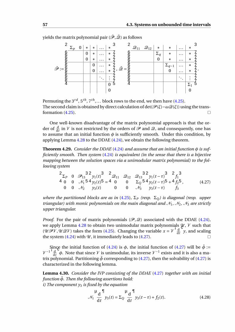
57 4.3. Systems on unbounded time intervals
yields the matrix polynomial pair (P ,Q) as follows
P :=
Σp 0 ∗ ∗ . . . ∗0 ∗ . . . ∗0 ∗ . . . ∗
0 . . . ∗0 . . . ∗
. . ....00
, Q =
Q11 Q12 ∗ ∗ . . . ∗Σq ∗ . . . ∗0 ∗ . . . ∗
Σq−1 . . . ∗0 . . . ∗
. . ....Σ1
0
.
Permuting the 3r d , 5th , 7th , . . . block rows to the end, we then have (4.25).The second claim is obtained by direct calculation of det(P (ξ)−ωQ(ξ)) using the trans-formation (4.25).
One well-known disadvantage of the matrix polynomial approach is that the or-der of d
dt in V is not restricted by the orders of P and Q, and consequently, one hasto assume that an initial function φ is sufficiently smooth. Under this condition, byapplying Lemma 4.28 to the DDAE (4.24), we obtain the following theorem.
Theorem 4.29. Consider the DDAE (4.24) and assume that an initial function φ is suf-ficiently smooth. Then system (4.24) is equivalent (in the sense that there is a bijectivemapping between the solution spaces via a unimodular matrix polynomial) to the fol-lowing systemΣP 0 P13
0 0 N1
0 0 N2
y1(t )y2(t )y3(t )
=Q11 Q12 Q13
0 0 ΣQ
0 0 N3
y1(t −τ)y2(t −τ)y3(t −τ)
+ f1
f2
f3
, (4.27)
where the partitioned blocks are as in (4.25), ΣP (resp. ΣQ ) is diagonal (resp. uppertriangular) with monic polynomials on the main diagonal and N1, N2, N3 are strictlyupper triangular.
Proof. For the pair of matrix polynomials (P ,Q) associated with the DDAE (4.24),we apply Lemma 4.28 to obtain two unimodular matrix polynomials U , V such that(UP V ,UQV ) takes the form (4.25). Changing the variable x = V
( ddt
)y , and scaling
the system (4.24) with U , it immediately leads to (4.27).
Since the initial function of (4.24) is φ, the initial function of (4.27) will be φ :=V −1( d
dt
)φ. Note that since V is unimodular, its inverse V −1 exists and it is also a ma-
trix polynomial. Partitioning φ corresponding to (4.27), then the solvability of (4.27) ischaracterized in the following lemma.
Lemma 4.30. Consider the IVP consisting of the DDAE (4.27) together with an initialfunction φ. Then the following assertions hold:i) The component y3 is fixed by the equation
N1
(d
dt
)y3(t ) =ΣQ
(d
dt
)y3(t −τ)+ f2(t ). (4.28)

4.3. Systems on unbounded time intervals 58
ii) The third equation of (4.27) provides a consistency condition for f3.iii) The second component y2 can be freely chosen, so it can be reinterpreted as an inputfunction.
Proof. The claims ii) and iii) are direct consequences of the claim i), so we only needto prove i). Rewriting equation (4.28) explicitly by utilizing the structure of N1 and ΣQ ,we have
0 ∗ . . . ∗0 . . . ∗
. . ....0
y3(t ) =
Σq ∗ . . . ∗
Σq−1 . . . ∗. . .
...Σ1
y3(t −τ)+ f2(t ),
where Σ j = diag(p j ,1, p j ,2, . . . , p j ,r j ) with monic p j ,1, p j ,2, . . . , p j ,r j ∈C1,1[ξ].
Partitioning y3 conformably as y3 =[
zTq zT
q−1 . . . zT1
]T, we can recursively solve for
the components z1, z2, . . . , zq , and hence we obtain y3.
By utilizing Theorem 4.29 and Lemma 4.30, we obtain the solvability properties ofthe DDAE (4.24) (and in particular, the DDAE (4.1a)). Besides that, the following corol-lary to Theorem 4.29 states that the DDAE (4.24) is regular if and only if the associatedpolynomial q(λ,ω) is not identically zero.
Corollary 4.31. Assume that an initial function x|[−τ,0] associated with the DDAE (4.24)is sufficiently smooth. Then the corresponding IVP for (4.24) has a unique solution forevery inhomogeneity f ∈C∞([0,∞),Cm) if and only if system (4.24) is of square size andthe associated polynomial q(λ,ω) is not identically zero.
Proof. [Necessity.] Due to Lemma 4.30, in the condensed form (4.27), the second blockcolumn and the last block row do not occur. Therefore, the DDAE (4.24) is of squaresize and
det(U )det(P (ξ)−ωQ(ξ))det(V ) = det
([Σp −ωQ11 P13 −ωQ13
0 N1 −ωΣQ
]).
Denote by q the size of ΣQ . Since U , V are unimodular, we have
det(P (ξ)−ωQ(ξ))
= (det(U ))−1 (det(V ))−1 det(ΣP −ωQ11) det
−ωΣq ∗ . . . ∗
−ωΣq−1 . . . ∗. . .
...−ωΣ1
= (det(U ))−1 (det(V ))−1 det(ΣP −ωQ11) (−ω)qq∏
i=1det(Σi ),
which clearly is a non-zero polynomial.[Sufficiency.] Assume that the associated polynomial q(λ,ω) is not identically zero.Thus, Lemma 4.28 implies the existence of two unimodular matrix polynomials U ,V such that UP V and UQV take the form (4.26).

59 4.3. Systems on unbounded time intervals
Changing the variable x = V( d
dt
)y and scaling (4.24) with U , we obtain the system
ΣP ∗ ∗ . . . ∗0 ∗ . . . ∗
0 ∗. . .
...0
y(t ) =
Q11 ∗ ∗ . . . ∗
Σq ∗ . . . ∗Σq−1 ∗
. . ....Σ1
y(t −τ)+U f (t ),
which is uniquely solvable, due to Lemma 4.30. Therefore, the DDAE (4.25) is regular.
In particular, the restriction of Corollary 4.31 to the DDAE (4.1a) gives us the fol-lowing corollary.
Corollary 4.32. Consider the IVP (4.1) for the DDAE (4.1a) and assume that an initialfunction φ is sufficiently smooth. Then the IVP (4.1) has a unique solution for everyinhomogeneity f ∈ C∞([0,∞),Cm) if and only if system (4.1a) is of square size and theassociated polynomial q(λ,ω) = det(λE − A−ωB) is not identically zero.
Remark 4.33. From Corollary 4.32, one sees that the regularity of a DDAE is indepen-dent of the (positive) delay τ. This property is important for control applications, forexample where one applies a time-delayed feedback control u(t ) = K x(t −τ) to a de-scriptor system of the form E x(t ) = Ax(t )+Bu(t ). There the delay τ is used as a pa-rameter to achieve a desired behavior of the descriptor system, and in general it isnecessary to verify the regularity of the closed-loop control system for each delay. Nev-ertheless, Corollary 4.32 shows that it suffices to verify the regularity of the system foran arbitrary delay.
4.3.3 Reformulation of non-advanced systems
In Subsection 4.3.2 we have studied DDAEs by using the matrix polynomial approach.However, this approach bears the following disadvantages:i) Both the inhomogeneity and an initial function are required to be sufficiently smooth.ii) It is more suitable for the theoretical investigation than for the numerical integra-tion.Therefore, another system reformulation of (4.1a) is desired. The importance of re-tarded and neutral systems in applications draws our attention to DDAEs of these twotypes. Therefore, we need the following assumption.
Assumption 4.34. The DDAE (4.1a) is of either retarded or neutral type.
In this subsection, we extend the algebraic approach presented in Section 2.2 tostudy DDAEs under the assumption that the matrix triple (E , A,B) is regular. To con-sider the associated polynomial det(λE − A −ωB), it is necessary to assume that theDDAE (4.1a) is square. The following lemma describes the resulting system by apply-ing Algorithm 2.1 to the DDAE (4.1a), under Assumption 4.34.
Lemma 4.35. Consider the DDAE (4.1a). Let µ be the strangeness index of the matrixpair (E , A). Furthermore, let Assumption 4.34 hold. Then, Algorithm 2.1 applied to

4.3. Systems on unbounded time intervals 60
(4.1a) gives the resulting systemE1
00
x(t ) =A1
A2
0
x(t )+B1
B2
B3
x(t −τ)+ 0
0B4
x(t −τ)+
f1(t )f2(t )f3(t )
,dµaµvµ
(4.29)
where[E T
1 AT2
]Tis of full row rank.
Proof. The proof is directly obtained by using Lemma 2.21, where the function x(t −τ)is considered as the function parameter.
From (4.29), one sees that the initial function φmust satisfy the consistency condi-tion
0 = B3φ(t −τ)+ B4φ(t −τ)+ f3(t ), (4.30)
for all t ∈ (0,τ). In this case, the DDAE (4.1a) has the same solution set as the equation E1
0−B4
x(t ) =A1
A2
B3
x(t )+B1
B2
0
x(t −τ)+
f1(t )f2(t )
f3(t +τ)
.dµaµvµ
(4.31)
Furthermore, since the strangeness-free formulation preserves the associated polyno-mial det(λE − A−ωB), one sees that
det(λE − A−ωB) = det
λE1
00
−A1
A2
0
−ωB1
B2
B3
−λω 0
0B4
= ωvµ det
λ E1
0−B4
−A1
A2
B3
−ωB1
B2
0
.
Thus, by transforming the DDAE (4.1a) to the new form (4.31), the degree ofω in the as-sociated polynomial decreases by vµ. Since the associated polynomial det(λE−A−ωB)is not identically zero, the degree of ω is finite. Thus, the following algorithm termi-nates after a finite number of iterations.
Algorithm 4.1
1: Input: The DDAE (4.1a). Set j = 0, E0 = E , A0 = A, B0 = B , f0(t ) = f (t ).2: Apply Algorithm 2.1 to the DDAE
E j x(t ) = A j x(t )+ B j x(t −τ)+ f j (t ),
to obtain system (4.29) and the characteristic quantities dµ, aµ, vµ.3: if vµ = 0 then STOP,4: else proceed to 6.5: end if

61 4.3. Systems on unbounded time intervals
6: Shift forward the last equation of (4.29) by τ to obtain (4.31). Increase j by 1, set
E j = E1
0−B4
, A j =A1
A2
B3
, B j =B1
B2
0
, f j (t ) =
f1(t )f2(t )
f3(t +τ)
,
and go back to 2.
Algorithm 4.1 applied to the DDAE (4.1a) results in the following theorem.
Theorem 4.36. Consider the IVP (4.1) for the square DDAE (4.1a). Let Assumption 4.34hold and assume that the matrix triple (E , A,B) is regular. Furthermore, suppose thatthe initial function φ satisfies the consistency condition (4.30) in every iterations of Al-gorithm 4.1. Then, the DDAE (4.1a) has the same solution set as the system[
Id 00 0
][y1(t )y2(t )
]=[
A11 00 Ia
][y1(t )y2(t )
]+[
B11 B12
B21 B22
][y1(t −τ)y2(t −τ)
]+[γ1(t )γ2(t )
], (4.32)
where x =Q y, for some nonsingular matrix Q ∈ Cn,n . Consequently, the IVP (4.1) has aunique solution.
Proof. The second claim is straightforward from the first one, since the correspondingIVP for the DDAE (4.32) has a unique solution. Therefore, we only need to prove thefirst claim. Applying Algorithm 4.1 to the DDAE (4.1a), we obtain the system[
E1
0
]x(t ) =
[A1
A2
]x(t )+
[B1
B2
]x(t −τ)+
[f1(t )f2(t )
], (4.33)
where[E T
1 AT2
]Tis nonsingular. Thus, there exists nonsingular matrices P , Q ∈ Cn,n
such that
P
[E1
0
]Q =[
Id 00 0
], P
[A1
A2
]Q =[
A11 00 Ia
].
Scaling system (4.33) with P and changing the variable x =Q y , one obtains the desiredform (4.32).
The consistency condition for the initial function φ is given by the following corol-lary.
Corollary 4.37. Consider the IVP (4.1) for the square DDAE (4.1a). Let Assumption 4.34hold and assume that the matrix triple (E , A,B) is regular. Then, the initial functionφ isconsistent if and only if the following conditions are satisfied.i) The identity (4.30) holds for every iteration of Algorithm 4.1.ii) The second block equation of (4.33) is satisfied at t = 0, which means that
A2(0)φ(0)+ B2(0)φ(−τ)+ f2(0) = 0.
Now let us illustrate the validity of Algorithm 4.1 and Theorem 4.36 by the followingexample.

4.3. Systems on unbounded time intervals 62
Example 4.38. Consider the DDAE[1 00 0
]︸ ︷︷ ︸
E
x(t ) =[
0 01 0
]︸ ︷︷ ︸
A
x(t )+[
1 00 −1
]︸ ︷︷ ︸
B
x(t −τ)+[
f1(t )f2(t )
], (4.34)
on the time interval [0,∞). The associated polynomial q(λ,ω) = (λ−ω)ω is not identi-cally zero, so the matrix triple (E , A,B) is regular. Algorithm 4.1 applied to (4.34) readsin detail.
• j = 0.• System (4.29) takes the form[
0 00 0
]x(t ) =
[0 01 0
]x(t )+
[1 00 −1
]x(t−τ)+
[0 −10 0
]x(t−τ)+
[f1(t )+ f2(t )
f2(t )
],
vµ = 1aµ = 1
.
Since vµ = 1 6= 0, we proceed to line 6 of Algorithm 4.1.• System (4.31) takes the form[
0 10 0
]x(t ) =
[1 01 0
]x(t )+
[0 00 −1
]x(t −τ)+
[f1(t +τ)+ f2(t +τ)
f2(t )
].
dµ = 1aµ = 1
• j= 1. Since vµ = 0, STOP.
Consequently, the formulation (4.32) in Theorem 4.36 is obtained by performing Gaus-sian elimination[
0 10 0
]x(t ) =
[0 01 0
]x(t )+
[0 10 −1
]x(t −τ)+
[f1(t +τ)+ f2(t +τ)− f2(t )
f2(t )
],
followed by a column permutation x(t ) =[
0 11 0
]y(t ).

Chapter 5
Solvability Analysis of General LinearTime Varying DDAEs
“Truth is ever to be found in the simplicity, and not in the multiplicity and confusion ofthings.”
Isaac NewtonCited in Rules for methodizing the Apocalypse, Rule 9, from a manuscript published in
The Religion of Isaac Newton (1974) by Frank E. Manuel, p. 120.
Having studied the theoretical properties of linear time invariant DDAEs in Chap-ter 4, the main goal of this chapter is to address the solvability of DDAEs in such a waythat it can be used later for the numerical integration of the IVP (1.2). Our object now isgeneral systems with linear time varying coefficients of the form (1.2a). As seen in Sec-tion 3.4, systems with multiple commensurate delays can be transformed into singledelay systems, and hence all the results in this chapter can also be extended withoutany difficulty to the multiple delay case. However, for notational simplicity we onlydiscuss the single delay case.
With the goal of the numerical solution to the IVP (1.2), we need to handle twoproblems. First, we must generalize the strangeness-free formulation (2.13) of non-delayed DAEs (Section 2.2) to DDAEs. Second, we must determine the smoothnessrequirements and the consistency conditions for an initial function φ and an inhomo-geneity f . Recall that for the IVP (1.2), we use the piecewise continuously differentiablesolution concept. Furthermore, we assume the existence and uniqueness of a solutionas follows.
Assumption 5.1. Assume that for any consistent inhomogeneity function f and anyconsistent initial function φ with respect to f , the IVP (1.2) has a unique solution.
Recall that by introducing new functions as in the method of steps, the DDAE (1.2a)can be rewritten as a sequence of DAEs
E j (t )x j (t ) = A j (t )x j (t )+B j (t )x j−1(t )+ f j (t ), j = 1, . . . ,`, (5.1)
for all t ∈ (0,τ), and due to the continuity of x at the points iτ, 16 i 6 `, we obtain
xi (0) = xi−1(τ), (5.2)
63

5.1. Generalization of the method of steps 64
for i = 1, . . . ,`, with the note that x0(τ) =φ(0).The failure of the method of steps for dealing with noncausal DDAEs, as have seen
in Section 3.3, motivates two new approaches:The first approach aims to generalize the method of steps, so that we can still computethe sequence of functions xi | i = 1, . . . ,` step by step, starting from x1. This approachwill be our main concern in Sections 5.1-5.3.The second approach is to rewrite the set of DAEs (5.1) as one DAE on the time inter-
val (0,τ) of the combined variable X = [xT1 . . . xT
`
]T. This DAE is coupled with the
boundary conditions (5.2) to form a differential-algebraic BVP. Thus, by computing X
from this BVP, we are able to determine all the functions xi , i = 1, . . . ,` not consecu-tively as the method of steps, but at the same time. This approach will be examined inSection 5.4. This chapter is completed with the comparison of these two approachesand some illustrative examples.
5.1 Generalization of the method of steps
Similar to the method of steps, the core of the generalization is the problem of deter-mining the solution x of the IVP (1.2) on the time interval [(i −1)τ, iτ], provided thatx is known on the interval [−τ, (i −1)τ]. This problem can be restated as determiningfunction xi , provided that functions xi−1, . . . , x0 are already known. Clearly, the subsetof (5.1) that contains the first i −1 DAEs
E j (t )x j (t ) = A j (t )x j (t )+B j (t )x j−1(t )+ f j (t ), j = 1, . . . , i −1,
becomes a set of redundant equations and as a result, the solvability of xi is governedby the set of DAEs
E j (t )x j (t ) = A j (t )x j (t )+B j (t )x j−1(t )+ f j (t ), j = i , . . . ,`. (5.3)
The failure of the method of steps for general DDAEs is due to the reason that it usesonly the first equation of system (5.3) (i.e., j = i ) to determine xi . Therefore, the naturalidea of a new method is computing xi (t ) from (5.3). Note that depending on the timeinterval, the set of DAEs (5.3) may have finite equations (` < ∞) or infinitely manyequations (` =∞). In the second case, one certainly cannot use the whole set (5.3) todetermine xi , and this fact motivates the shift index concept in the next definition.
Definition 5.2. For a fixed i 6 `, consider the set of DAEs (5.3). The minimum numberk ∈N0 such that the so-called shift-inflated system
Ei+ j (t )xi+ j (t ) = Ai+ j (t )xi+ j (t )+Bi+ j (t )xi+ j−1(t )+ fi+ j (t ), j = 0, . . . ,k, (5.4)
has a unique solution xi , provided a function xi−1 and a consistent initial vectorxi (0) = xi−1(τ), is called the shift index of the set of DAEs (5.1) with respect to i , andbe denoted by κ(i ).
The idea for a generalization of the method of steps is carried out in the next algo-rithm.

65 5.1. Generalization of the method of steps
Algorithm 5.1 Generalization of the method of steps
1: Input: The IVP (1.2) for the linear DDAE (1.2a).2: Return: The solution x on consecutive time intervals [(i −1)τ, iτ], 16 i 6 `.3: Rewrite the IVP (1.2) as a sequence of DAEs (5.1) by the method of steps.4: for i = 1 to ` do5: Set k = 0.6: Construct the shift-inflated DAE system (5.4).7: Determine whether one can compute xi uniquely from (5.4).8: if YES then κ(i ) = k, solve xi from (5.4),9: else increase k by 1 and go back to 6.
10: end if11: end for
We demonstrate the applicability of Algorithm 5.1 in the next example.
Example 5.3. Consider the DDAE[1 00 0
]x(t ) =
[0 01 0
]x(t )+
[0 10 0
]x(t −τ)+
[f (t )g (t )
],
for all t ∈ (0,∞). The DAE sequence (5.1) reads[1 00 0
]xi (t ) =
[0 01 0
]xi (t )+
[0 10 0
]xi−1(t )+
[fi (t )gi (t )
], (5.5)
for i = 1, 2, . . . . Let us fix some i ∈N and see how Algorithm 5.1 proceeds to compute xi .1.) With k = 0, the set of DAEs (5.4) is nothing else than the DAE (5.5). However, one caneasily see that the function xi is not uniquely determined from (5.5), so this fact meansthat: first, the method of steps fails to compute xi , and second, the shift index κ(i ) mustbe bigger than zero. Now we increase k by 1 and go back to line 6 of Algorithm 5.1.2.) With k = 1, the set (5.4) reads[
1 00 0
]xi (t ) =
[0 01 0
]xi (t )+
[0 10 0
]xi−1(t )+
[fi (t )gi (t )
], (5.6a)
[1 00 0
]xi+1(t ) =
[0 01 0
]xi+1(t )+
[0 10 0
]xi (t )+
[fi+1(t )gi+1(t )
]. (5.6b)
Adding the derivative of the second equation of (5.6b) to its first equation, it follows that
0 = [0 1]
xi (t )+ fi+1(t )+ gi+1(t ),
which gives an explicit formula for the second component of xi . On the other hand, thefirst component of xi is clearly fixed by the second equation of (5.6a) and therefore system(5.6) uniquely determines xi . Thus, the shift index κ(i ) is 1 for all i . More important, weobserve that to compute xi numerically, one must work with the system (5.6), which isunder-determined for the variable xi+1. We, however, do not care about this since ourfunction of interest xi is still uniquely computable.
Now we discuss the critical part of Algorithm 5.1: How to verify the unique solvabil-
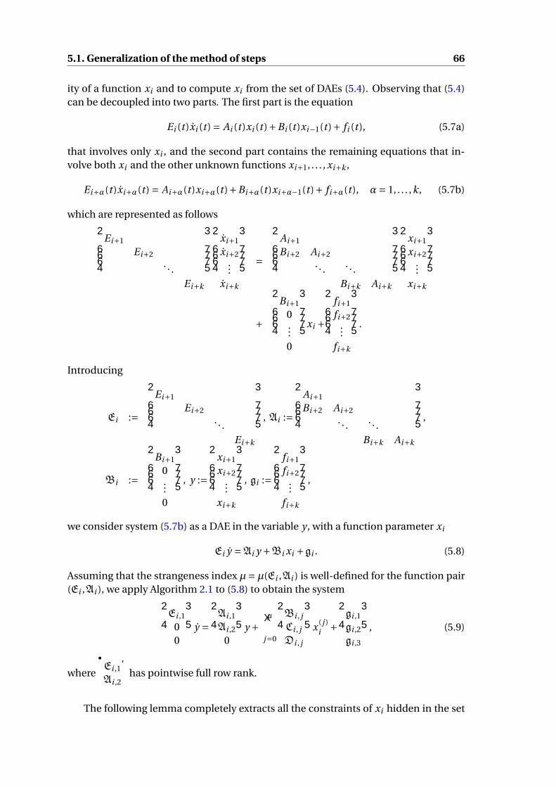
5.1. Generalization of the method of steps 66
ity of a function xi and to compute xi from the set of DAEs (5.4). Observing that (5.4)can be decoupled into two parts. The first part is the equation
Ei (t )xi (t ) = Ai (t )xi (t )+Bi (t )xi−1(t )+ fi (t ), (5.7a)
that involves only xi , and the second part contains the remaining equations that in-volve both xi and the other unknown functions xi+1, . . . , xi+k ,
Ei+α(t )xi+α(t ) = Ai+α(t )xi+α(t )+Bi+α(t )xi+α−1(t )+ fi+α(t ), α= 1, . . . ,k, (5.7b)
which are represented as followsEi+1
Ei+2. . .
Ei+k
xi+1
xi+2...
xi+k
=
Ai+1
Bi+2 Ai+2. . . . . .
Bi+k Ai+k
xi+1
xi+2...
xi+k
+
Bi+1
0...0
xi +
fi+1
fi+2...
fi+k
.
Introducing
Ei :=
Ei+1
Ei+2. . .
Ei+k
, Ai :=
Ai+1
Bi+2 Ai+2. . . . . .
Bi+k Ai+k
,
Bi :=
Bi+1
0...0
, y :=
xi+1
xi+2...
xi+k
, gi :=
fi+1
fi+2...
fi+k
,
we consider system (5.7b) as a DAE in the variable y , with a function parameter xi
Ei y =Ai y +Bi xi +gi . (5.8)
Assuming that the strangeness index µ=µ(Ei ,Ai ) is well-defined for the function pair(Ei ,Ai ), we apply Algorithm 2.1 to (5.8) to obtain the systemEi ,1
00
y =Ai ,1
Ai ,2
0
y +µ∑
j=0
Bi , j
Ci , j
Di , j
x( j )i +
gi ,1
gi ,2
gi ,3
, (5.9)
where
[Ei ,1
Ai ,2
]has pointwise full row rank.
The following lemma completely extracts all the constraints of xi hidden in the set

67 5.1. Generalization of the method of steps
of DAEs (5.4). More important, these extracted constraints give us the sufficient andnecessary condition for the unique solvability of xi .
Lemma 5.4. Consider a fixed number i ∈ N, 1 6 i 6 `, and assume that the functionxi−1 is known. Furthermore, assume that the strangeness index µ is well-defined for theDAE (5.8). Then all the constraints of xi hidden in the set of DAEs (5.4) are given by thefollowing high-order DAE in the variable xi[
0Di ,µ
]x(µ)
i +·· ·+[
0Di ,2
]x(2)
i +[
Ei
Di ,1
]xi +[−Ai
Di ,0
]xi =[
Bi
0
]xi−1 +
[fi
−gi ,3
]. (5.10)
Here the functions Di , j , j = 0, . . . ,µ and gi ,3 come out from the system (5.9). Conse-quently, xi is uniquely determined from the set of DAEs (5.4) if and only if it is uniquelydetermined from the DAE (5.10).
Proof. First note that the strangeness-free formulation (5.9) does not alter the solutionset of the DAE (5.8) and consequently, xi is uniquely determined from the set of DAEs(5.4) if and only if it is also uniquely determined from the system
Ei xi = Ai xi +Bi xi−1 + fi , (5.11a)
Ei ,1 y = Ai ,1 y +µ∑
j=0Bi , j x( j )
i +gi ,1, (5.11b)
0 = Ai ,2 y +µ∑
j=0Ci , j x( j )
i +gi ,2, (5.11c)
0 =µ∑
j=0Di , j x( j )
i +gi ,3. (5.11d)
Since
[Ei ,1
Ai ,2
]has pointwise full row rank, we see that in the system (5.11b)-(5.11c) xi
only plays the role of a function parameter. Therefore, all the constraints of xi are givenby the two equations (5.11a) and (5.11d), which form the DAE (5.10).
Remark 5.5. i) Even though system (5.8) looks like a control system (a descriptor sys-tem), one should not confuse the strangeness-free formulation for a DAE [75] with theone for a descriptor system [76]. Here xi is specified as a function parameter, and it willnot be reinterpreted as a part of a new behavior variable as in [76].ii) We further note that since µ= µ(Ei ,Ai ), so in general µ depends on i . However, fornotational convenience, we will write µ instead of µ(i ).
From Lemma 5.4, we can deduce the existence and uniqueness of the shift index,even if `=∞, in the next theorem.
Theorem 5.6. Consider the IVP (1.2) and the sequence of functions xi | 1 6 i 6 ` aris-ing from applying the generalized method of steps to (1.2a). Let Assumption 5.1 hold.Furthermore, suppose that for each 16 i 6 ` the strangeness indices are well-defined forthe two DAEs (5.8) and (5.10). Then for each 1 6 i 6 `, there exists a unique shift indexκ(i ) for the set of DAEs (5.1) with respect to i .

5.1. Generalization of the method of steps 68
Proof. Consider a fixed i . From Lemma 5.4, we see that for each k ≥ 0, the set of DAEs(5.4) has the same solution xi as the DAE (5.10). Let uk be the number of undeterminedvariables contained in the solution x of the DAE (5.10), we then obtain a sequenceuk k≥0. Introducing
Mk := xi : [0,τ] →Cn | there exist functions xi+1, . . . , xi+k that satisfy (5.4),
Nk := xi : [0,τ] →Cn | xi solves the DAE (5.10),
we see thatMk =Nk for every k ≥ 0 due to Lemma 5.4.Since the sequence Mk k≥0 is decreasing in the sense that for every k we have Mk+1 ⊆Mk , so is the sequence Nk k≥0 and hence the sequence uk k≥0 is decreasing. Theboundedness from below of the sequence uk k≥0 implies that this sequence becomesstationary.Moreover, due to Assumption 5.1, the set of DAEs (5.4) has a unique solution for somek 6 `− i , no matter whether ` is finite or not. Therefore lim
k↑(`−i )uk = 0 and hence, there
exists a finite number k such that uk = 0. Let κ(i ) := mink ≥ 0 | uk = 0, we obtain theexistence and uniqueness of the shift index κ(i ) for the set of DAEs (5.1).
Remark 5.7. It would be ideal if in (5.10) we have Di , j = 0 for all j ≥ 2. Then, with theinitial vector xi (0) = xi−1(τ), one can compute xi by solving the corresponding IVP forthe first order DAE [
Ei
Di ,1
]xi +[−Ai
Di ,0
]xi =
[Bi
0
]xi−1 +
[fi
−gi ,3
].
However, in general, as pointed out in [65], a high-order constraint for x may be hiddenin (1.2a), which results in a high-order DAE (5.10). This situation is demonstrated inExample 5.8 below.
Example 5.8. Consider the IVP consisting of the DDAE0 0 10 0 00 1 0
x(t )y(t )z(t )
=0 1 0
0 0 10 0 0
x(t )y(t )z(t )
+0 0 0
1 0 00 0 0
x(t −1)y(t −1)z(t −1)
+ −t−1−e t−1
1
, (5.12)
on the time interval I= [0,∞), together with an initial function[x(t ) y(t ) z(t )
]T = [φ1(t ) φ2(t ) φ3(t )]T
, t ∈ [−1,0].
Applying Algorithm 5.1 to (5.12), we have the set of DAEs where the i th-DAE, i ∈N, reads0 0 10 0 00 1 0
xi (t )yi (t )zi (t )
=0 1 0
0 0 10 0 0
xi (t )yi (t )zi (t )
+0 0 0
1 0 00 0 0
xi−1(t )yi−1(t )zi−1(t )
+ −t − i +1−1−e t+i−2
1
, (5.13)
for t ∈ (0,1). One sees that for every i , the function xi is not uniquely determined from(5.13) and hence, κ(i ) > 0. Thus, we proceed to the line 9 of Algorithm 5.1. Constructingthe set of DAEs (5.4) with k = 1 and applying Lemma 5.4, we obtain the DAE (5.10) which

69 5.1. Generalization of the method of steps
reads0 0 10 0 00 1 0
xi (t )yi (t )zi (t )
=0 1 0
0 0 10 0 0
xi (t )yi (t )zi (t )
+0 0 0
1 0 00 0 0
xi−1(t )yi−1(t )zi−1(t )
+ −t − i +1−1−e t+i−2
1
,
0 = xi (t )−e t+i−1,
which clearly implies the existence and uniqueness of[xi yi zi
]T. As a result, the shift
index is κ(i ) = 1 and the DAE (5.10) is a second order DAE.
This high-order situation, however, does not lead to any theoretical difficulty, sincethe analysis of high-order DAEs has been studied in Section 2.3. By utilizing Theorem2.23 and Corollaries 2.25, 2.26 for the DAE (5.10), we can deduce the strangeness-freeDDAE of the variable xi in the following theorem.
Theorem 5.9. Consider the IVP (1.2) and the sequence of functions xi | 1 6 i 6 ` aris-ing from applying the generalized method of steps to (1.2a). Let Assumption 5.1 hold.Furthermore, suppose that for each 16 i 6 ` the strangeness indices are well-defined forthe two DAEs (5.8) and (5.10). Then, for each i , the function xi is also the solution of thestrangeness-free DDAE
Aiµ,1 Ai
µ−1,1 . . . Ai0,1
Aiµ−1,2 . . . Ai
0,2. . .
...Ai
0,µ+1
0 0 . . . 0
x(µ)(t )x(µ−1)(t )
...x(t )
=
B iη,1 B i
η−1,1 . . . B i0,1
B iη,2 B i
η−1,2 . . . B i0,2
......
...B iη,µ+1 B i
η−1,µ+1 . . . B i0,µ+1
B iη,µ+2 B i
η−1,µ+2 . . . B i0,µ+2
x(η)(t −τ)
x(η−1)(t −τ)...
x(t −τ)
+
f i1
f i2...
f iµ+1
f iµ+2
, (5.14)
with some µ, η ∈N0, where the matrix-valued function
Aµ
i :=[(
Aiµ,1
)T (Aiµ−1,2
)T. . .(
Ai0,µ+1
)T ]T
is pointwise nonsingular. Furthermore, some of the block rows may not be present.
Proof. By applying Theorem 2.23 to the DAE (5.10), we obtain the strangeness-freeDDAE (5.14), where Aµ
i has pointwise full row rank. Furthermore, due to the unique-
ness of the function xi , it turns out that the matrix function Aµ
i is pointwise nonsingu-lar.
Analogous to Corollary 2.25, the restriction of an underlying DDE of (1.2a) on thetime interval [(i − 1)τ, iτ] is derived from the strangeness-free DDAE (5.14) as in thenext corollary.

5.2. Solvability analysis via system classification 70
Corollary 5.10. Consider the IVP (1.2) and the sequence of functions xi | 16 i 6 ` aris-ing from applying the generalized method of steps to (1.2a). We further assume that foreach i , all the required conditions in Theorem 5.9 are satisfied, so that the strangeness-free DDAE (5.14) is well-defined. Then, the restriction of the underlying DDE for theDDAE (1.2a) on the interval [(i −1)τ, iτ] is of the form
µ∑α=0
Aαi (t )x(α)(t ) =
η+µ−1∑α=0
Bαi (t )x(α)(t )+ gi (t ), (5.15)
where Aµ
i is pointwise nonsingular.
Proof. As in Corollary 2.25, the underlying DDE (5.15) is obtained by differentiating thei th block row equation of (5.14) exactly µ−i times and changing back the time variablet 7→ t + (i −1)τ.
From the strangeness-free DDAE (5.14), by choosing i = 1 one obtains the neces-sary consistency condition for an initial function φ.
Corollary 5.11. Consider the IVP (1.2) and the sequence of functions xi | 1 6 i 6 `arising from applying the generalized method of steps to (1.2a). We further assume thatall the conditions in Theorem 5.9 are satisfied, so that the strangeness-free DDAE (5.14)is well-defined for every i . Then the necessary condition for a consistent initial functionφ is
0 =η∑
i=0B 1
i ,µ+2(t )φ(i )(t −τ)+ f 1µ+2(t ), (5.16)
for all t ∈ (0,τ).
Proof. Choosing i = 1, the last block equation of (5.14) gives the constraint
0 = B 1η,µ+2x(µ)
0 + B 1η−1,µ+2x(µ−1)
0 +·· ·+ B 10,µ+2x0 + f 1
µ+2.
which is exactly (5.16) since x0(t ) =φ(t −τ).
Example 5.12. Revisiting Example 5.8, the constraint (5.16) reads
0 = [1 0 0]φ(t −τ)−e t ,
for all t ∈ (0,τ).
5.2 Solvability analysis via system classification
As stated in Remark 2.30, in most applications, the mathematical models are describedby DDAEs of either retarded or neutral type. Furthermore, inherited from the theoryof DDEs, it is reasonable to restrict a considered DDAE to either a retarded or a neutralsystem. Thus, within this section, we assume the following.
Assumption 5.13. The DDAE (1.2a) is of either retarded or neutral type.
Under Assumption 5.13, Lemma 5.4 can be significantly improved as follows.

71 5.2. Solvability analysis via system classification
Lemma 5.14. Let Assumption 5.13 hold for the DDAE (1.2a). Under the conditions ofLemma 5.4, the DAE (5.10) becomes[
Ei
−Di ,1
]xi =
[Ai
Di ,0
]xi +[
Bi
0
]xi−1 +
[fi
gi ,3
]. (5.17)
Proof. Since Assumption 5.13 is satisfied, it implies that the parameter dependent DAE(5.8) is of non-advanced type. Therefore, Lemma 2.21 applied to (5.8) results in thesystem Ei ,1
00
y =Ai ,1
Ai ,2
0
y +Bi ,0
Ci ,0
Di ,0
xi + 0
0Di ,1
xi +gi ,1
gi ,2
gi ,3
,
and hence we obtain the desired form (5.17).
Now let us reinterpret system (5.17) as a DAE in variable xi with the function parameterxi−1. Due to Assumption 5.13, one sees that the function xi is either smoother or assmooth as the function parameter xi−1. Therefore, (5.17) is also a non-advanced DAE.Applying Lemma 2.21 to the DAE (5.17), we can further simplify the DAE (5.17) as inthe following lemma.
Lemma 5.15. Consider the DDAE (1.2a) and the sequence of functions xi | 1 6 i 6 `arising from applying the generalized method of steps to (1.2a). Let Assumptions 5.1,5.13 hold. Then, for each i ≥ 1, the function xi is also the solution of the strangeness-freeDAE Ei ,1
00
xi =Ai ,1
Ai ,2
0
xi +Bi ,1
Bi ,2
Bi ,3
xi−1 + 0
0Bi ,4
xi−1 +gi ,1
gi ,2
gi ,3
,di
ai
vi
(5.18)
where the matrix function[
E Ti ,1 AT
i ,2
]Tis pointwise nonsingular. The sizes of the block
rows in (5.18) are di , ai , vi . Furthermore, if the DDAE (1.2a) is retarded, then Bi ,2 = 0and Bi ,4 = 0.
Proof. Applying the strangeness-free formulation in Algorithm 2.1 to the DAE (5.17),
Lemma 2.21 implies the desired system (5.18), where the matrix function[
E Ti ,1 AT
i ,2
]T
has pointwise full row rank. Furthermore, from Assumption 5.1, we see that the DAE
(5.17) has a unique solution xi and it implies that the matrix function[
E Ti ,1 AT
i ,2
]Tis
pointwise nonsingular.
Notice that not only the function coefficients but also the sizes of the block rows in thestrangeness-free DAE (5.18) depend on i . Considering (5.18) and defining new func-tions
Ei ,1(t ) := Ei ,1(t − (i −1)τ),
Ai , j (t ) := Ai , j (t − (i −1)τ), j = 1, 2,
Bi , j (t ) := Bi , j (t − (i −1)τ), j = 1, 2, 3, 4,
gi , j (t ) := gi , j (t − (i −1)τ), j = 1, 2, 3,

5.2. Solvability analysis via system classification 72
for t ∈ [(i −1)τ, iτ], i = 1, . . . ,`, then the generalization of the strangeness-free formula-tion (2.13) to DDAEs is given in the following theorem.
Theorem 5.16. Consider the DDAE (1.2a) and let Assumptions 5.1, 5.13 hold. Then, foreach 1 6 i 6 `, the restricted function x|[(i−1)τ,iτ] is also the solution of the strangeness-free DDAEEi ,1(t )
00
x(t )=Ai ,1(t )
Ai ,2(t )0
x(t )+Bi ,1(t )
Bi ,2(t )Bi ,3(t )
x(t −τ)+ 0
0Bi ,4(t )
x(t −τ)+gi ,1(t )gi ,2(t )gi ,3(t )
,di
ai
vi(5.19)
where the matrix function[
E Ti ,1 AT
i ,2
]Tis pointwise nonsingular. The sizes of the block
rows in (5.19) are di , ai and vi . Furthermore, if the DDAE (1.2a) is retarded, then Bi ,2 = 0and Bi ,4 = 0 for all i = 1, . . . ,`.
Proof. The proof follows directly from Lemma 5.15, since (5.19) is nothing else than(5.18) with a changed variable t 7→ t + (i −1)τ.
Under the conditions of Theorem 5.16, we see that the first two block rows of thestrangeness-free DDAE (5.19) gives us a system that uniquely determines the functionx|[(i−1)τ,iτ], provided that the restricted function x|[(i−2)τ,(i−1)τ] is known. Thus, we callthe system [
Ei ,1(t )0
]x(t )=
[Ai ,1(t )Ai ,2(t )
]x(t )+
[Bi ,1(t )Bi ,2(t )
]x(t −τ)+
[gi ,1(t )gi ,2(t )
], (5.20)
the regular, strangeness-free formulation of the DDAE (1.2a).
Considering system (5.19) in the case i = 1, we obtain the necessary conditions fora consistent initial function φ in the following corollary.
Corollary 5.17. Consider the DDAEs (1.2a), (5.19) and let Assumptions 5.1, 5.13 hold.Then, the necessary condition for a consistent initial function φ is as follows.i) If (1.2a) is of retarded type then φ has to satisfy the conditions
A1,2(0)φ(0)+ g1,2(0) = 0,
B1,3(t )φ(t −τ)+ g1,3(t ) = 0, for all t ∈ (0,τ),(5.21a)
ii) If (1.2a) is of neutral type then φ has to satisfy the conditions
A1,2(0)φ(0)+ B1,2(0)φ(−τ)+ g1,2(0) = 0,
B1,3(t )φ(t −τ)+ B1,4(t )φ(t −τ)+ g1,3(t ) = 0, for all t ∈ (0,τ).(5.21b)
Furthermore, the smoothness requirement for φ is that φ ∈ C 0 (resp. φ ∈ C 1) in the casethat the DDAE (1.2a) is retarded (resp. neutral).
Proof. The proof is obtained directly by letting i = 1 in (5.19) and note that in the re-tarded case, we have B1,2 = 0 and B1,4 = 0, due to Theorem 5.16.

73 5.3. Regularization of DDAEs by operational arrays
In order to see the difference between DAEs and different classes of DDAEs more clearly,we summarize the results about the strangeness-free formulation and the consistencyinitial condition for DAEs as well as for DDAEs in Tables 5.1, 5.2.
System type Regular, strangeness-free formulationrestricted to [(i −1)τ, iτ], 16 i 6 `
DAEs
[E1(t )
0
]x(t )−
[A1(t )A2(t )
]x(t ) =
[f1(t )f2(t )
],
where[E T
1 AT2
]is pointwise nonsingular.
Causal DDAEs
[E1(t )
0
]x(t )=
[A1(t )A2(t )
]x(t )+
[B0,1(t )B0,2(t )
]x(t −τ)
+µ∑
i=1
[0
Bi ,2(t )
]x(i )(t −τ)+
[f1(t )f2(t )
],
where[E T
1 AT2
]is pointwise nonsingular.
General retarded DDAEs
[Ei ,1(t )
0
]x(t ) =
[Ai ,1(t )Ai ,2(t )
]x(t )+
[Bi ,1(t )
0
]x(t −τ)+
[gi ,1(t )gi ,2(t )
],
where[
E Ti ,1 AT
i ,2
]is pointwise nonsingular.
General neutral DDAEs
[Ei ,1(t )
0
]x(t ) =
[Ai ,1(t )Ai ,2(t )
]x(t )+
[Bi ,1(t )Bi ,2(t )
]x(t −τ)+
[gi ,1(t )gi ,2(t )
],
where[
E Ti ,1 AT
i ,2
]is pointwise nonsingular.
General advanced DDAEs The strangeness-free formulation takes the form (5.14).The underlying DDE takes the form∑µα=0 Aα
i (t )x(α)(t ) =∑η+µ−1α=0 Bα
i (t )x(α)(t −τ)+ gi (t ),
where Aµ
i is pointwise nonsingular and there exists at leastone function Bα
i , i ≥µ+1, that is not identically zero.
Table 5.1: Strangeness-free formulation for different classes of DDAEs.
5.3 Regularization of DDAEs by operational arrays
In Section 5.2, we have seen that the generalized method of steps applied to retardedand neutral DDAEs results in the regular, strangeness-free DDAE (5.20). For the nu-merical solution, it is necessary to determine this equation pointwise, and that is themain purpose of this section. In order to do that, we make use of two operational ar-rays:
i) The shift operation that maps the DDAE (1.2a) into the equation
E(t +τ)x(t +τ) = A(t +τ)x(t +τ)+B(t +τ)x(t )+ f (t +τ).
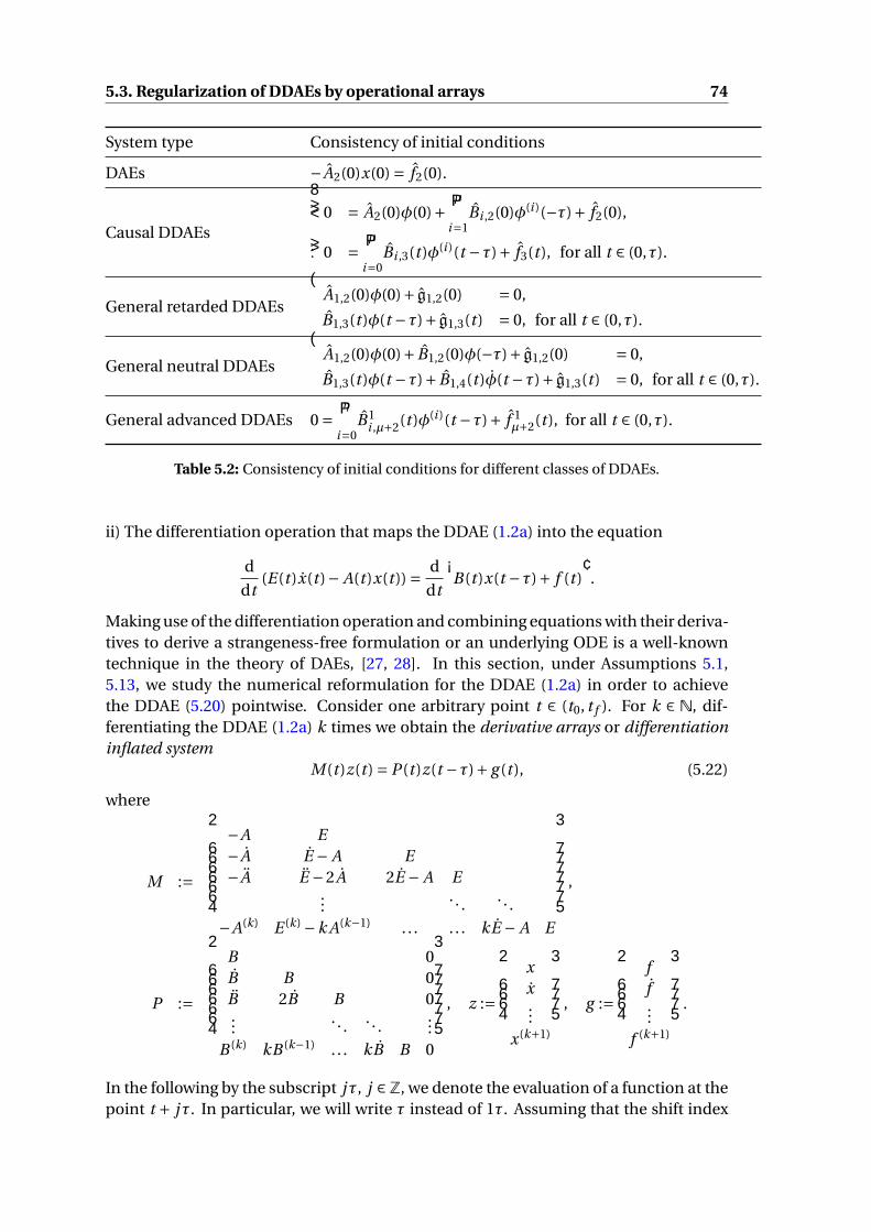
5.3. Regularization of DDAEs by operational arrays 74
System type Consistency of initial conditions
DAEs −A2(0)x(0) = f2(0).
Causal DDAEs
0 = A2(0)φ(0)+
µ∑i=1
Bi ,2(0)φ(i )(−τ)+ f2(0),
0 =µ∑
i=0Bi ,3(t )φ(i )(t −τ)+ f3(t ), for all t ∈ (0,τ).
General retarded DDAEs
A1,2(0)φ(0)+ g1,2(0) = 0,
B1,3(t )φ(t −τ)+ g1,3(t ) = 0, for all t ∈ (0,τ).
General neutral DDAEs
A1,2(0)φ(0)+ B1,2(0)φ(−τ)+ g1,2(0) = 0,
B1,3(t )φ(t −τ)+ B1,4(t )φ(t −τ)+ g1,3(t ) = 0, for all t ∈ (0,τ).
General advanced DDAEs 0 =η∑
i=0B 1
i ,µ+2(t )φ(i )(t −τ)+ f 1µ+2(t ), for all t ∈ (0,τ).
Table 5.2: Consistency of initial conditions for different classes of DDAEs.
ii) The differentiation operation that maps the DDAE (1.2a) into the equation
d
dt(E(t )x(t )− A(t )x(t )) = d
dt
(B(t )x(t −τ)+ f (t )
).
Making use of the differentiation operation and combining equations with their deriva-tives to derive a strangeness-free formulation or an underlying ODE is a well-knowntechnique in the theory of DAEs, [27, 28]. In this section, under Assumptions 5.1,5.13, we study the numerical reformulation for the DDAE (1.2a) in order to achievethe DDAE (5.20) pointwise. Consider one arbitrary point t ∈ (t0, t f ). For k ∈ N, dif-ferentiating the DDAE (1.2a) k times we obtain the derivative arrays or differentiationinflated system
M(t )z(t ) = P (t )z(t −τ)+ g (t ), (5.22)
where
M :=
−A E−A E − A E−A E −2A 2E − A E
.... . . . . .
−A(k) E (k) −k A(k−1) . . . . . . kE − A E
,
P :=
B 0B B 0B 2B B 0...
. . . . . ....
B (k) kB (k−1) . . . kB B 0
, z :=
xx...
x(k+1)
, g :=
ff...
f (k+1)
.
In the following by the subscript jτ, j ∈Z, we denote the evaluation of a function at thepoint t + jτ. In particular, we will write τ instead of 1τ. Assuming that the shift index

75 5.3. Regularization of DDAEs by operational arrays
κ is well-defined and that it is a constant for all t ∈ I, the shift-inflated system (5.4) isthen given by
E0τx0τ = A0τx0τ+B0τx−τ+ f0τ,Eτxτ = Aτxτ+Bτx0τ+ fτ,E2τx2τ = A2τx2τ+B2τxτ+ f2τ,
...Eκτxκτ = Aκτxκτ+Bκτx(κ−1)τ+ fκτ.
(5.23)
In order to build the derivative array of system (5.23), one needs to rewrite (5.23) asE0τ
EτE2τ
. . .Eκτ
x0τ
xτx2τ
...xκτ
=
A0τ
Bτ Aτ
B2τ A2τ. . . . . .
Bκτ Aκτ
x0τ
xτx2τ
...xκτ
+
B0τx−τ+ f0τ
fτf2τ...
fκτ
.
(5.24)Let us suppose that for the DAE (5.24), the strangeness index µ(t ) is well-defined andbecomes a constant in a sufficiently small neighborhood B(t ) of t . Now we can buildthe derivative arrays with k = µ(t ) for the DAE (5.24). However, to reduce the cost in thedetermination of the shift indexκ, it would be better to build the derivative arrays (withk = µ(t )) for the equations of system (5.23) instead of building the derivative arraysfor the entire system (5.24). Following this way, we have the so-called double-inflatedsystem
M0τ
−Pτ Mτ
−P2τ M2τ. . . . . .
−Pκτ Mκτ
z0τ
zτz2τ
...zκτ
=
P0τ
00...0
z−τ+
g0τ
gτg2τ
...gκτ
. (5.25)
We denote the matrix coefficients of (5.25) as
M :=
M0τ
−Pτ Mτ
−P2τ M2τ. . . . . .
−Pκτ Mκτ
, P :=
P0τ
00...0
, G :=
g0τ
gτg2τ
...gκτ
. (5.26)
Here one should not confuse P with the matrix polynomial P in Subsection 4.3.2.Within this section, we do not consider any matrix polynomial. We discuss now howto derive the regular, strangeness-free DDAE (5.20) from the double-inflated system(5.25).
Remark 5.18. It should be noted that due to the non-causality of the DDAE (1.2a), thedifferential equations of the regular, strangeness-free DDAE (5.20) must be selectedfrom the double-inflated system (5.25), instead of from the original DDAE (1.2a). Thisis in contrast to both cases of non-delayed DAEs and of causal DDAEs. We illustrate

5.3. Regularization of DDAEs by operational arrays 76
this fact in the next example.
Example 5.19. Consider the IVP consisting of the DDAE[1 00 0
][x(t )y(t )
]=[
0 01 0
][x(t )y(t )
]+[
0 00 −1
][x(t −τ)y(t −τ)
]+[
e t
−e t + t −τ]
, (5.27)
for t ∈ [0,∞), τ= 1, with an initial function φ(t ) :=[
e t
t
], for t ∈ [−τ,0].
By directly checking, we obtain κ= 1 and the regular, strangeness-free DDAE (5.35) is[0 −10 0
][x(t )y(t )
]=[
0 01 0
][x(t )y(t )
]+[
0 00 −1
][x(t −τ)y(t −τ)
]+[ −1−e t + t −τ
].
Clearly, the differential equation 0 = [0 −1][x(t )
y(t )
]− 1 cannot be selected from the
original DDAE (5.27).
From Remark 5.18, we see that it is necessary to select all the constraints for x(t )and x(t ) contained in (5.25). It is worth to note that x(t ) and x(t ) are only presentin z0τ but not in zτ, . . . , zκτ. In the following, for notational convenience, we will useMatlab notation, [91].
Let the matrix U be such that its columns span the space corangeM (:, (2n +1) : end),i. e.,
U T M (:, (2n +1) : end) = 0. (5.28)
By scaling (5.25) with U T , we obtain the system
U T M (:,1 : 2n)
[x(t )x(t )
]=U T P z−τ+U TG, (5.29)
that contains all the constraints for x(t ) and x(t ) in (5.25).
We further notice that in the DDAE (5.20) only x(t−τ) occurs even though z−τ containsnot only x(t −τ) but also its derivatives x(t −τ), x(t −τ), . . . . Thus, the matrix U shouldbe chosen to satisfy the additional condition
U T P (:, (n +1) : end) = 0. (5.30)
In the case that U T P (:, (n+1) : end) 6= 0, it implies that the DDAE (1.2a) is of advancedtype, and hence Assumption 5.13 is violated.Denote by
M :=U T M (:, (n +1) : 2n), N :=U T M (:,1 : n), P :=U T P (:,1 : n), G :=U TG, (5.31a)
and let m be the number of rows of the matrix function M . Thus M , N , P are matri-ces of size m by n. We consider the following spaces and matrices
Z2 basis of corange(M ) = ker(M T ),T2 basis of ker(Z T
2 N ),Z1 basis of range(MT2).
(5.31b)

77 5.3. Regularization of DDAEs by operational arrays
On the one hand, the algebraic constraints of the DDAE (5.20) are contained in theresulting system obtained by scaling system (5.29) with Z T
2 as
Z T2 N x(t ) = Z T
2 P x(t −τ)+Z T2 G . (5.32)
On the other hand, the set of differential equations in the DDAE (5.20) are containedin the resulting system obtained by scaling system (5.29) with Z T
1 as
Z T1 M x(t )+Z T
1 N x(t ) = Z T1 P x(t −τ)+Z T
1 G . (5.33)
Thus, the fact that the regular, strangeness-free DDAE (5.20) is contained in the cou-pled system (5.32), (5.33) implies that
rank
[Z T
1 M
Z T2 N
]= n.
Furthermore, we still need to remove some equations in (5.32) and (5.33), due to thefact that Z T
2 N and Z T1 M may not have full row rank. Therefore, we consider the fol-
lowing spaces and matrices
Y2 basis of range(Z T2 N ),
Y1 basis of range(Z T1 M ).
(5.34)
Scaling (5.32) (resp., (5.33)) with Y T2 (resp. Y T
1 ), we see that the DDAE (5.20) becomes[Y T
1 Z T1 M
0
]x(t )+
[Y T
1 Z T1 N
Y T2 Z T
2 N
]x(t ) =
[Y T
1 Z T1 P
Y T2 Z T
2 P
]x(t −τ)+
[Y T
1 Z T1 G
Y T2 Z T
2 G
], (5.35)
where
[Y T
1 Z T1 M
Y T2 Z T
2 N
]is nonsingular.
In summary, the regularization of the IVP (1.2) by using operational arrays is pro-posed in Algorithm 5.2 below.
Algorithm 5.2 Regularization of the IVP (1.2)
1: Input: The IVP (1.2).2: Return: The regular, strangeness-free DDAE (5.20) pointwise.3: Let κ= 0.4: Construct the double-inflated system (5.25) with the coefficients M , P , G as in
(5.26).5: Let the matrix U be such that the conditions (5.28), (5.30) hold.6: Compute the matrices M , N , Z2, T2, Z1, Y1, Y2 as in (5.31) and (5.34).7: if
rank
([Z T
1 M
Z T2 N
])= n,
then (5.35) is exactly the regular, strangeness-free DDAE (5.20).8: else κ := κ+1, go back to 4.9: end if

5.3. Regularization of DDAEs by operational arrays 78
Let us demonstrate Algorithm 5.2 by studying the following example.
Example 5.20. Consider the IVP consisting of the DDAE[1 00 0
][x(t )y(t )
]=[
0 01 0
][x(t )y(t )
]+[
0 10 0
][x(t −τ)y(t −τ)
]+[
1−et−τ10
−t
], (5.36)
for t ∈ [0,∞), τ= 1, with an initial function φ(t ) :=[
t
et
10
], for t ∈ [−τ,0].
Applying Algorithm 5.2 to (5.36), we proceed as follows.
With κ= 0 we obtain
U =
0 −1 01 0 00 0 00 0 1
, M = 0 0
−1 0−1 0
, N = −1 0
0 00 0
,
Z2 = 0.7071 0.7071
0.5000 −0.5000−0.5000 0.5000
, T2 =[
01
], Z1 = [ ]3,0,
Z T2 N =
[0.7071 00.7071 0
], Z T
1 M = [ ]0,2.
Here by [ ]i , j we denote the empty matrix of the size i by j .
Thus, rank
([Z T
1 M
Z T2 N
])= 1 < 2, which implies that the shift index is bigger than 0 (equiv-
alently, the DDAE (5.36) is noncausal).
With κ= 1 we obtain
M =
0 0−1 0−1 00 0
, N =
0 −0.70710 00 0−1 0
, P =
0 00 00 −10 0
,
Z2 =
0.7071 0.7071 00.5000 −0.5000 0−0.5000 0.5000 0
0 0 1.0000
, T2 = [ ]2,0, Z1 = [ ]4,0,
Z T2 N =
0 0.50000 0.5000
1.0000 0
, Z T1 M = [ ]0,2,Y1 = [ ]0,0, Y2 =
0 −0.70710 −0.7071
−1.0000 0
.
In this case rank
([Z T
1 M
Z T2 N
])= 2 and therefore the shift index is κ= 1. The DDAE (5.35)
is [0 00 0
][x(t )y(t )
]=[−1 0
0 −0.7071
][x(t )y(t )
]+[
0 00 0
][x(t −τ)y(t −τ)
]+[
t
0.7071 et
10
].

79 5.4. Boundary Value Problem method
Remark 5.21. For linear time invariant DDAEs, the functions M , P , G, Z2, T2, Z1, Y1,Y2 can be chosen to be constant matrices on the whole interval. Therefore, we onlyneed to compute them at the initial point and can use them in the whole integrationprocess.
Note that Algorithm 5.2 is successfully applied to the DDAE (1.2a) if and only if thefollowing conditions hold:
i) Assumptions 5.1, 5.13 are satisfied.ii) The strangeness index is well-defined for the DAE (5.24) so that we can derive the
regular, strangeness-free DDAE (5.20).In more detail, we formulate the following hypothesis to guarantee that Algorithm 5.2can be performed and the regular, strangeness-free DDAE (5.20) can be achieved.
Hypothesis 5.22. Consider the DDAE (1.2a). Suppose that there exist integers κ, a, msuch that for each t ∈ I, the strangeness index µ(t ) is well-defined for the DAE (5.24) in asufficiently small neighborhood B(t ) of t , and the functions M , P , obtained by buildingthe derivative arrays with k = µ(t ) as in (5.26), satisfy the following properties:
1. There exists a smooth, full rank matrix function U of size (κ+1)(µ+1)n by msuch that its columns span the space corange(M (:, (2n +1) : end)) andU T P (:, (n +1) : end) = 0. We set
M :=U T M (:, (n +1) : 2n), N :=U T M (:,1 : n).
2. There exists a smooth matrix function Z2 of size m by a on B(t ), such that Z T2 M =
0 and Z T2 N has pointwise full row rank a.
3. There exists a smooth matrix function T2 of size n by d := n − a, and T2 haspointwise maximal rank such that Z T
2 N T2 = 0.4. For all s ∈B(t ), we have rank(M (s)T2(s)) = d so that there exists a smooth, point-
wise maximal rank matrix function Z1 of size m by d satisfyingrank(Z T
1 (s)M (s)T2(s)) = d .
As noted in Section 3.3, in the case of advanced DDAEs, the order µ (resp., η) of x(t )(resp., x(t −τ)) in the strangeness-free formulation (5.14) can be arbitrarily high, andtherefore it is complicated to determine system (5.14) pointwise. Furthermore, evenif system (5.14) is already known, it will be hard and can be inefficient to implementnumerical methods like Runge-Kutta or BDF methods to (5.14). Therefore, anotherapproach is needed to determine whether it is possible to integrate an advanced DDAE.This is the main purpose of the BVP method presented in the next section.
5.4 Boundary Value Problem method
In this section we examine a second approach to investigate the solvability of the IVP(1.2), the Boundary Value Problem method (BVP method). The main idea is to trans-form IVPs for DDAEs into BVPs for DAEs in order to remove the delay τ and to be ableto make use of results for differential-algebraic BVPs. To do that, we introduce new se-quences of functions as in (5.1) and rewrite the IVP (1.2) as a sequence of DAEs on the

5.4. Boundary Value Problem method 80
time interval (0,τ)
E j (t )x j (t ) = A j (t )x j (t )+B j (t )x j−1(t )+ f j (t ), j = 1, . . . ,`. (5.37)
However, unlike Algorithm 5.1, we do not solve the sequence of IVPs for the DAEs (5.37)step by step. Instead, we rewrite the IVP (1.2) as the differential-algebraic BVP for thefollowing DAE of size `m ×`n
E1(t )E2(t )
. . .E`(t )
x1(t )x2(t )
...x`(t )
=
A1(t )B2(t ) A2(t )
. . . . . .B`(t ) A`(t )
x1(t )x2(t )
...x`(t )
+
B1(t )x0(t )+ f1(t )
f2(t )...
f`(t )
, for all t ∈ (0,τ),
(5.38a)
together with the boundary conditionIn
0 In. . . . . .
0 In
x1(0)x2(0)
...x`(0)
+
0−In 0
. . . . . .−In 0
x1(τ)x2(τ)
...x`(τ)
=φ(0)
0...0
. (5.38b)
Let us introduce new notation and rewrite the BVP (5.38) in a compact form as
E (t )X (t ) =A (t )X (t )+B(t )x0(t )+F (t ), for all t ∈ (0,τ), (5.39a)
C X (0)+DX (τ) =~v , (5.39b)
with X (t ) = [xT1 (t ) xT
2 (t ) . . . xT`
(t )]T
and ~v := [φT (0) 0 . . . 0]T
.Assuming that the strangeness index µ = µ(E ,A ) is well-defined for the DAE (5.39a)and applying Algorithm 2.1 to (5.39a), one obtains the strangeness-free DAE
E1(t )00
X (t ) =A1(t )
A2(t )0
X (t )+
∑µ
j=0 B1, j (t )x( j )0 (t )+F1(t )∑µ
j=0 B2, j (t )x( j )0 (t )+F2(t )∑µ
j=0 B3, j (t )x( j )0 (t )+F3(t )
, (5.40)
where
[E1(t )A2(t )
]has pointwise full row rank.
By studying the solution X to the BVP (5.39), we derive the solvability of the IVP (1.2)in the following theorem.
Theorem 5.23. Consider the IVP (1.2) on the bounded time interval I= [t0, t0 +`τ). As-sume that the strangeness indexµ=µ(E ,A ) is well-defined for the DAE (5.39a) with thestrangeness-free formulation (5.40). Moreover, let Assumption 5.1 hold. Then we have:i) The initial function φ is consistent if and only if φ is µ-times continuously differen-
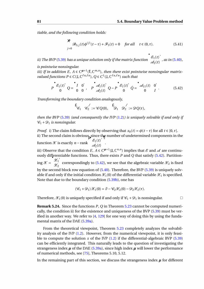
81 5.4. Boundary Value Problem method
tiable, and the following condition holds:
µ∑j=0
B3, j (t )φ( j )(t −τ)+F3(t ) = 0 for all t ∈ (0,τ). (5.41)
ii) The BVP (5.39) has a unique solution only if the matrix function
[E1(t )A2(t )
], as in (5.40),
is pointwise nonsingular.iii) If in addition E, A ∈ Cµ+1(I,Cm,n), then there exist pointwise nonsingular matrix-valued functions P ∈C (I,C`n,`n), Q ∈C 1(I,C`n,`n) such that
P
[E1(t )
0
]Q =[
I 00 0
], P
[A1(t )A2(t )
]Q −P
[E1(t )
0
]Q =[A11(t ) 0
0 I
]. (5.42)
Transforming the boundary condition analogously,[C1 C2
]:=C Q(0),
[D1 D2
]:=DQ(τ),
then the BVP (5.39) (and consequently the IVP (1.2)) is uniquely solvable if and only ifC1 +D1 is nonsingular.
Proof. i) The claim follows directly by observing that x0(t ) =φ(t −τ) for all t ∈ [0,τ].ii) The second claim is obvious, since the number of undetermined components in the
function X is exactly n − rank
([E1(t )A2(t )
]).
iii) Observe that the condition E , A ∈ Cµ+1(I,Cn,n) implies that E and A are continu-ously differentiable functions. Thus, there exists P and Q that satisfy (5.42). Partition-
ing X =[X1
X2
]correspondingly to (5.42), we see that the algebraic variable X2 is fixed
by the second block row equation of (5.40). Therefore, the BVP (5.39) is uniquely solv-able if and only if the initial condition X1(0) of the differential variable X1 is specified.Note that due to the boundary condition (5.39b), one has
(C1 +D1)X1(0) =~v −C2X2(0)−D2X2(τ).
Therefore, X1(0) is uniquely specified if and only if C1 +D1 is nonsingular.
Remark 5.24. Since the functions P , Q in Theorem 5.23 cannot be computed numeri-cally, the condition ii) for the existence and uniqueness of the BVP (5.39) must be ver-ified in another way. We refer to [4, 129] for one way of doing this by using the funda-mental matrix of the DAE (5.39a).
From the theoretical viewpoint, Theorem 5.23 completely analyzes the solvabil-ity analysis of the IVP (1.2). However, from the numerical viewpoint, it is only feasi-ble to compute the solution x of the IVP (1.2) if the differential-algebraic BVP (5.39)can be efficiently integrated. This naturally leads to the question of investigating thestrangeness index µ of the DAE (5.39a), since high index µ will lower the performanceof numerical methods, see [75], Theorems 5.10, 5.12.
In the remaining part of this section, we discuss the strangeness index µ for different

5.4. Boundary Value Problem method 82
types of the DDAE (1.2a). Certainly, the BVP method is expected to work for retardedor neutral systems. We consider one special case of (1.2a) in the next proposition.
Proposition 5.25. Consider the DDAE (1.2a) and assume that the following conditionshold.i) The matrix function pair (E , A) is sufficiently smooth with a well-defined strangenessindex µ and characteristic quantities dµ, aµ, vµ, uµ that satisfy vµ = uµ = 0.ii) Assumptions 5.1, 5.13 hold.Then, the DAE (5.39a) has a well-defined strangeness index which is exactly µ.
Proof. Due to the condition i), we see that for each j = 1, . . . ,`, the DAE
E j (t )x j (t ) = A j (t )x j (t )+B j (t )x j−1(t )+ f j (t ), (5.43)
is regular and has a well-defined strangeness index µ. This means that if B j (t )x j−1(t )+f j ∈ Cµ+1([0,τ],Cn) then x j is continuously differentiable. This condition is furtherrelaxed by Assumption 5.13, which implies that only f j is required to be µ+ 1 timescontinuously differentiable, but x j−1 only needs to be continuously differentiable.Therefore, by simple induction, one sees that if x0 ∈C 1([0,τ],Cn) and f j ∈Cµ+1([0,τ],Cn)for all j = 1, . . . ,`, there exists uniquely ` functions x1, . . . , x` ∈ C 1([0,τ],Cn) that solvethe DAE sequence (5.43). This implies that the DAE (5.39a) has a well-defined strangenessindex µ.
Remark 5.26. It is worth to note that if one removes the condition vµ = uµ = 0 in condi-tion i) of Proposition 5.25, then the DAE (5.39a) can have a strangeness index µ biggerthan µ, as demonstrated in the next example.
Example 5.27. Consider the Delay-DAE[0 10 0
]︸ ︷︷ ︸
E
x(t ) =[
1 00 0
]︸ ︷︷ ︸
A
x(t )+[
0 00 1
]︸ ︷︷ ︸
B
x(t −τ)+[
f1(t )f2(t )
](5.44)
on the time interval [0,2τ]. Algorithm 5.2 applied to (5.44) results in the strangeness-freeDDAE [
0 00 0
]x =[
0 11 0
]x(t )+
[f2(t +τ)
f1(t )+ f2(t +τ)
].
The underlying DDE of (5.44) therefore is[0 11 0
]x(t ) =−
[f2(t +τ)
f1(t )+ f2(t +τ)
],
is of retarded type, and hence the DDAE (5.44) is of retarded type. One also sees that thestrangeness index of the pair (E , A) is µ(E , A) = 0 and the characteristic quantities aredµ = 1, aµ = 0, vµ = 0, uµ = 1.

83 5.4. Boundary Value Problem method
The BVP approach, however, leads to the matrix function pair (E ,A ) given by
E =
0 1 0 00 0 0 00 0 0 10 0 0 0
, A =
1 0 0 00 0 0 00 0 1 00 1 0 0
,
and the strangeness index of the pair (E ,A ) is µ(E ,A ) = 1, which is bigger than thestrangeness µ(E , A). Therefore the BVP method can increase the strangeness index, evenin the case that the considered DDAE is non-advanced.
Now let us turn to the case that the DDAE (1.2a) is of advanced type.
Example 5.28. Consider the following DDAE on the time interval (0,`τ)[0 10 0
]︸ ︷︷ ︸
E
[x(t )y(t )
]=[
1 00 1
]︸ ︷︷ ︸
A
[x(t )y(t )
]−[
0 0λ 0
]︸ ︷︷ ︸
B
[x(t −τ)y(t −τ)
]+[
f1(t )f2(t )
], (5.45)
with a parameter λ ∈ R. By adding the derivative of the second equation to the firstequation, we obtain 0 = x(t )−λx(t −τ)+ g (t ), where g (t ) := f2(t )+ f1(t ). Thus, (5.45)is of retarded type (resp., advanced type) if λ = 0 (resp., λ 6= 0). Now we consider thestrangeness index µ of the pair (E ,A ) for different value of λ.i) With λ= 0, one sees that
E = diag(E ,E , . . . ,E), A = diag(A, A, . . . , A).
One can directly find that the Kronecker index ν of the pair (E ,A ) is equal to the Kro-necker index of the pair (E , A). It therefore implies that the two pairs (E ,A ) and (E , A)have the same strangeness index.ii) For λ = 1 the constraint 0 = x(t )−λx(t −τ)+ g (t ) implies that x(t ) = x(t −τ)− g (t ).Thus, for any t ∈ ((i −1)τ, iτ) we have
x(t ) = [1 0]φ(i )(t − iτ)−
i−1∑j=0
λ j g ( j )(t − jτ).
As a consequence,
x`(t ) = [1 0]φ(`)(t − (`−1)τ)−
`−1∑j=0
λ j g ( j )(t − jτ),
which yields that the strangeness index of the matrix function pair (E ,A ) is `.
Example 5.28 demonstrates that if the DDAE (1.2a) is of advanced type, the DAE (5.39a)may have an arbitrarily high index. This situation leads to very poor performance oreven divergence of numerical methods whenever the desired integration time intervalis long. In this case, the numerical error is rapidly amplified in time, as shown in Figure5.1 below. Here the inhomogeneity f is chosen such that the system possesses the
analytical solution
[x(t )y(t )
]=[
te t/10
]. The simulation is done by using the 3 stage Radau

5.4. Boundary Value Problem method 84
IIA method of [130] with constant step size h = 0.01 for system (5.45) with λ= 1.
0 2 4 6 8 1010−20
10−10
100
1010errory
0 2 4 6 8 1010−10
10−4
102
108 errorx
Figure 5.1: Absolute error vs. length of the time interval I for (5.45).
The advantage of the BVP method is that even if the DDAE (1.2a) is of advancedtype, the numerical solution to the IVP (1.2) can still be efficiently computed, providedthat the strangeness indexµ is sufficiently small. This fact is illustrated in the followingexample.
Example 5.29. Consider the IVP (1.2) for the DDAE[0 10 0
]︸ ︷︷ ︸
E
[x(t )y(t )
]=[
1 00 1
]︸ ︷︷ ︸
A
[x(t )y(t )
]−[
0 00 1
]︸ ︷︷ ︸
B
[x(t −τ)y(t −τ)
]+[
f1(t )f2(t )
], (5.46)
on the time interval (0,`τ) for some integer ` ∈ N. The inhomogeneity is chosen such
that the system possesses the analytical solution
[x(t )y(t )
]=[
te t/10
].
Adding the derivative of the second equation of (5.46) to the first equation and elimi-nating x on both sides, one obtains[
00
]=[
x(t )y(t )
]−[
0 00 1
][x(t −τ)y(t −τ)
]−[
0 10 0
][x(t −τ)y(t −τ)
]+[
f1(t )+ f2(t )f2(t )
], (5.47)
and therefore the DDAE (5.46) is of advanced type.Furthermore, by direct computation, one can verify that the strangeness index µ of thepair (E ,A ) is exactly 1. For illustration, we consider `= 10 which leads to the numericalsolution and absolute error presented in Figure 5.2. The simulation is done by using thethree stage Radau IIA method of [130] with constant step size h = 0.01 for system (5.46).
So far in this chapter we have presented two different approaches to analyze thesolvability analysis of general linear time varying DDAEs. We compare these two ap-proaches in Table 5.3.
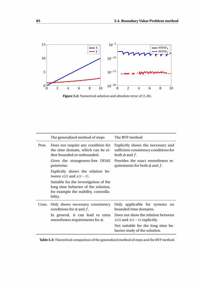
85 5.4. Boundary Value Problem method
0 2 4 6 8 1010−20
10−15
10−10
10−5errorxerrory
0 2 4 6 8 100
5
10
15xy
Figure 5.2: Numerical solution and absolute error of (5.46).
The generalized method of steps The BVP method
Pros. Does not require any condition forthe time domain, which can be ei-ther bounded or unbounded.
Explicitly shows the necessary andsufficient consistency conditions forboth φ and f .
Gives the strangeness-free DDAEpointwise.
Provides the exact smoothness re-quirements for both φ and f .
Explicitly shows the relation be-tween x(t ) and x(t −τ).
Suitable for the investigation of thelong time behavior of the solution,for example the stability, controlla-bility.
Cons. Only shows necessary consistencyconditions for φ and f .
Only applicable for systems onbounded time domains.
In general, it can lead to extrasmoothness requirements for φ.
Does not show the relation betweenx(t ) and x(t −τ) explicitly.
Not suitable for the long time be-havior study of the solution.
Table 5.3: Theoretical comparison of the generalized method of steps and the BVP method.

5.4. Boundary Value Problem method 86

Chapter 6
Numerical solutions of IVPs for DDAEs
This chapter is devoted to the numerical solution of the IVP (1.2). In view of Chapter 5,the theoretical solvability of (1.2) can be completely analyzed via either the generalizedmethod of steps (Algorithm 5.1) or the BVP method. In this chapter, these approachesare implemented and examined consecutively in Sections 6.1 and 6.2. Finally, someillustrative numerical experiments are presented.
Within this chapter, we assume that the (integration) time interval I is bounded, i.e.,`<∞, and that the IVP (1.2) has a unique solution x on I.
6.1 Application of the generalized method of stepsfor DDAEs
The integration strategy presented in this section is based on the theoretical results ofSections 5.1-5.3 under Assumption 5.13, i.e., the DDAE (1.2a) is of either retarded andneutral type. The main idea is that we do not directly integrate the original DDAE (1.2a)but instead we integrate the strangeness-free formulation (5.35) which takes the form[
E1(t )0
]x(t ) =
[A1(t )A2(t )
]x(t )+
[B1(t )B2(t )
]x(t −τ)+
[γ1(t )γ2(t )
], (6.1)
where
[E1
A2
]is pointwise invertible.
Recall that in Section 5.3, we have presented in Algorithm 5.2 an efficient approach tocompute the strangeness-free DDAE (5.35) pointwise in a stable way. In parallel to thepointwise determination of (5.35), by checking the condition (5.30) we can also ver-ify whether Assumption 5.13 holds, i.e., the type of the DDAE (1.2a) is not advanced.Therefore, the remaining work now is to integrate the system (6.1).Due to the presence of the delay term, it is necessary to calculate a dense output ratherthan a discrete approximation to the solution for evaluating the solution at the lagpoints. This requirement is attainable by interpolation or even better, by continuousmethods, see e.g. [13]. Due to this reason, the collocation methods seem to be goodcandidates. Adopted from the solver RADAR5 [60], we use the Radau scheme for the
87

6.1. Application of the generalized method of steps for DDAEs 88
numerical integration, which is given by nodes
0 < δ1 < ·· · < δs = 1, s ∈N. (6.2)
Since the DDAE (1.2a) is assumed to be of either retarded or neutral type and the delayτ is constant, we know all the discontinuity points that may occur in advance. Weinclude all the discontinuity points of x, x, . . . , x(s) into the mesh and denote a mesh by
π : t0 < t1 < ·· · < tN = t f . (6.3)
It should be noted that the number N in this chapter is the number of mesh points,which should not be confused with the nilpotent matrix N in the Kronecker-Weierstraßcanonical form.With the mesh π as in (6.3), the collocation points therefore are
ti j = ti +hiδ j , j = 1, . . . , s, (6.4)
where hi is the stepsize used at the i -th step. For the numerical approximation of thesolution, we seek for the piecewise polynomial Xπ of degree s, i.e., Xπ,i := Xπ|[ti ,ti+1] arepolynomials of degree s, which are determined by the following set of equations[
E1(ti j )0
]Xπ(ti j ) =
[A1(ti j )A2(ti j )
]Xπ(ti j )+
[B1(ti j )B2(ti j )
]Xπ(ti j −τ)+
[γ1(ti j )γ2(ti j )
], (6.5)
for all i = 1, . . . , N , j = 1, . . . , s.
If the delay factor
[B1(ti j )B2(ti j )
]Xπ(ti j − τ) does not occur, then (6.5) represents a linear
system for the internal stages Xπ,i (ti j ), j = 1, . . . , s for each i = 1, . . . ,`. Otherwise, in
the case that
[B1(ti j )B2(ti j )
]Xπ(ti j −τ) is present in (6.5), then we still have to define the past
function Xπ(ti j −τ) which is an approximation to x(ti j −τ). For this we choose
Xπ(ti j −τ) =φ(ti j −τ) if ti j −τ6 0,
Xπ,k (ti j −τ) for some 16 k 6 N that satisfies tk < ti j −τ6 tk+1.
The continuous output polynomial Xπ,k at the k-th step is given by Lagrange interpo-lation of order s, i.e.,
Xπ,k (tk +θhk ) =s∑
j=0L j (θ)Xπ,k (tk +δ j hk ), (6.6)
where L j (θ) is the Lagrange polynomial of degree s satisfying L j (δk ) = δk j with δk j
being the Kronecker delta symbol.
Remark 6.1. As noticed in [59, 60], one can optionally replace the continuous outputpolynomial Xπ,k in (6.6) by another dense output polynomial given by
Xπ,k (tk +θhk ) =s∑
j=1L j (θ)Xπ,k (tk +δ j hk ).
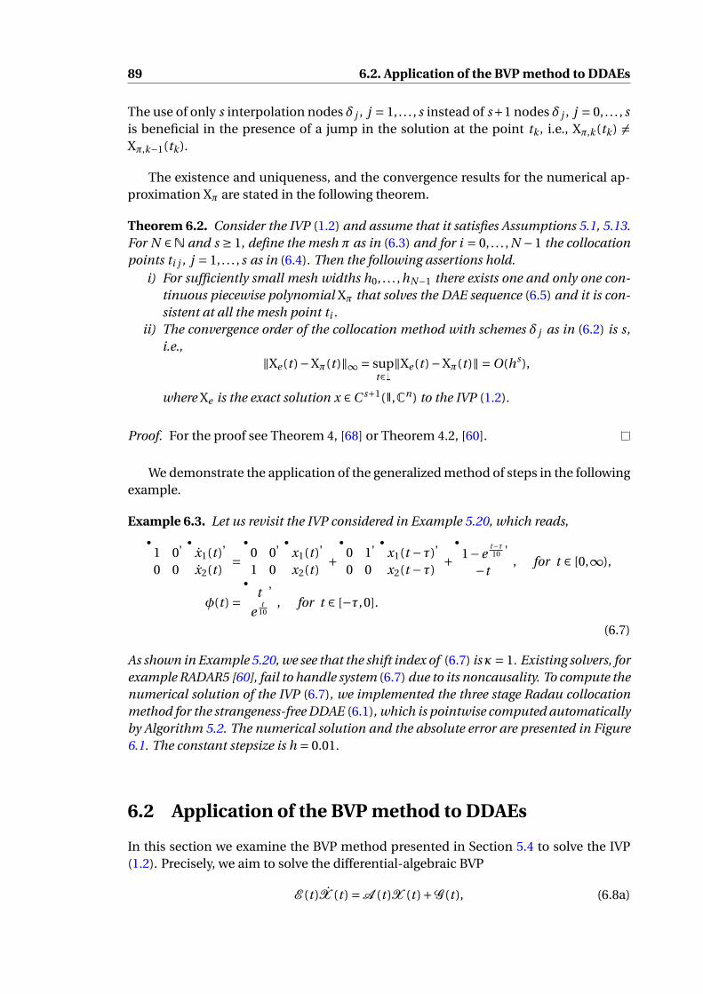
89 6.2. Application of the BVP method to DDAEs
The use of only s interpolation nodes δ j , j = 1, . . . , s instead of s+1 nodes δ j , j = 0, . . . , sis beneficial in the presence of a jump in the solution at the point tk , i.e., Xπ,k (tk ) 6=Xπ,k−1(tk ).
The existence and uniqueness, and the convergence results for the numerical ap-proximation Xπ are stated in the following theorem.
Theorem 6.2. Consider the IVP (1.2) and assume that it satisfies Assumptions 5.1, 5.13.For N ∈N and s ≥ 1, define the mesh π as in (6.3) and for i = 0, . . . , N −1 the collocationpoints ti j , j = 1, . . . , s as in (6.4). Then the following assertions hold.
i) For sufficiently small mesh widths h0, . . . ,hN−1 there exists one and only one con-tinuous piecewise polynomial Xπ that solves the DAE sequence (6.5) and it is con-sistent at all the mesh point ti .
ii) The convergence order of the collocation method with schemes δ j as in (6.2) is s,i.e.,
‖Xe (t )−Xπ(t )‖∞ = supt∈I
‖Xe (t )−Xπ(t )‖ =O(hs),
where Xe is the exact solution x ∈C s+1(I,Cn) to the IVP (1.2).
Proof. For the proof see Theorem 4, [68] or Theorem 4.2, [60].
We demonstrate the application of the generalized method of steps in the followingexample.
Example 6.3. Let us revisit the IVP considered in Example 5.20, which reads,[1 00 0
][x1(t )x2(t )
]=[
0 01 0
][x1(t )x2(t )
]+[
0 10 0
][x1(t −τ)x2(t −τ)
]+[
1−et−τ10
−t
], for t ∈ [0,∞),
φ(t ) =[
t
et
10
], for t ∈ [−τ,0].
(6.7)
As shown in Example 5.20, we see that the shift index of (6.7) isκ= 1. Existing solvers, forexample RADAR5 [60], fail to handle system (6.7) due to its noncausality. To compute thenumerical solution of the IVP (6.7), we implemented the three stage Radau collocationmethod for the strangeness-free DDAE (6.1), which is pointwise computed automaticallyby Algorithm 5.2. The numerical solution and the absolute error are presented in Figure6.1. The constant stepsize is h = 0.01.
6.2 Application of the BVP method to DDAEs
In this section we examine the BVP method presented in Section 5.4 to solve the IVP(1.2). Precisely, we aim to solve the differential-algebraic BVP
E (t )X (t ) =A (t )X (t )+G (t ), (6.8a)

6.2. Application of the BVP method to DDAEs 90
0 2 4 6 8 100
2
4
6
8
10
x1x2
0 2 4 6 8 1010−16
10−15
10−14
10−13
error x1error x2
Figure 6.1: Numerical solution and absolute error of the IVP (6.7) with constant stepsizeh = 0.01.
for all t ∈ (0,τ), with the boundary condition
C X (0)+DX (τ) = [φ(0) 0 . . . 0]T
, (6.8b)
where X (t ) = [xT (t ) xT (t +τ) . . . xT (t + (`−1)τ)]T
and the function coefficientsare
E (t ) =
E1(t )
E2(t ). . .
E`(t )
, A (t ) =
A1(t )B2(t ) A2(t )
. . . . . .B`(t ) A`(t )
,
G (t ) =
B1(t )φ(t −τ)+ f1(t )
f2(t )...
f`(t )
, C =
10 1
. . . . . .0 1
, D =
0−1 0
. . . . . .−1 0
.
As we have seen in Example 5.28, in the case that the DDAE (1.2a) is of advanced type,the matrix function pair (E ,A ) can have a very high index which is proportional to thelength of the time interval I. Therefore, we mainly focus on a solver which is incapableof efficiently integrating retarded and neutral DDAEs, and also advanced DDAEs thatsatisfy µ(E ,A )6 3.Similar to the generalized method of steps, we do not directly integrate the differential-algebraic BVP (6.8), but first we reformulate it into its strangeness-free formulation,and then apply numerical methods to this reformulated system.Algorithm 2.1 applied to system (6.8a) results in the strangeness-free DAEE1(t )
00
X (t ) =A1(t )
A2(t )0
X (t )+G1(t )
G2(t )G3(t )
, (6.9)
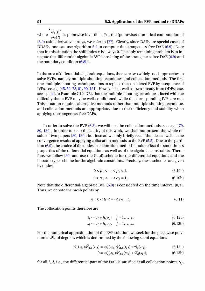
91 6.2. Application of the BVP method to DDAEs
where
[E1(t )A2(t )
]is pointwise invertible. For the (pointwise) numerical computation of
(6.9) using derivative arrays, we refer to [77]. Clearly, since DAEs are special cases ofDDAEs, one can use Algorithm 5.2 to compute the strangeness-free DAE (6.9). Notethat in this situation the shift index κ is always 0. The only remaining problem is to in-tegrate the differential-algebraic BVP consisting of the strangeness-free DAE (6.9) andthe boundary condition (6.8b).
In the area of differential-algebraic equations, there are two widely used approaches tosolve BVPs, namely multiple shooting techniques and collocation methods. The firstone, multiple shooting technique, aims to replace the considered BVP by a sequence ofIVPs, see e.g. [45, 52, 78, 81, 90, 121]. However, it is well-known already from ODEs case,see e.g. [4], or Example 7.10, [75], that the multiple shooting technique is faced with thedifficulty that a BVP may be well-conditioned, while the corresponding IVPs are not.This situation requires alternative methods rather than multiple shooting technique,and collocation methods are appropriate, due to their efficiency and stability whenapplying to strangeness-free DAEs.
In order to solve the BVP (6.3), we will use the collocation methods, see e.g. [79,80, 130]. In order to keep the clarity of this work, we shall not present the whole re-sults of two papers [80, 130], but instead we only briefly recall the idea as well as theconvergence results of applying collocation methods to the BVP (5.5). Due to the parti-tion (6.9), the choice of the nodes in collocation method should reflect the smoothnessproperties of the differential equations as well as of the algebraic constraints. There-fore, we follow [80] and use the Gauß scheme for the differential equations and theLobatto-type scheme for the algebraic constraints. Precisely, these schemes are givenby nodes
0 < ρ1 < ·· · < ρs < 1, (6.10a)
0 <σ1 < ·· · <σs = 1. (6.10b)
Note that the differential-algebraic BVP (6.8) is considered on the time interval [0,τ].Thus, we denote the mesh points by
π : 0 < t1 < ·· · < tN = τ. (6.11)
The collocation points therefore are
ti j = ti +hiρ j , j = 1, . . . , s, (6.12a)
si j = ti +hiσ j , j = 1, . . . , s. (6.12b)
For the numerical approximation of the BVP solution, we seek for the piecewise poly-nomial Xπ of degree s which is determined by the following set of equations
E1(ti j )Xπ,i (ti j ) =A1(ti j )Xπ,i (ti j )+G1(ti j ), (6.13a)
0 =A2(si j )Xπ,i (si j )+G2(si j ), (6.13b)
for all i , j , i.e., the differential part of the DAE is satisfied at all collocation points ti j ,

6.2. Application of the BVP method to DDAEs 92
and the algebraic part at all collocation points si j ,
T H2 (ti )
(Xπ,i (ti )−Xπ,i−1(ti )
)= 0, (6.13c)
for all i = 1, . . . , N −1, where columns of T H2 span the null space of A2 pointwise, i.e.,
the differential part of Xπ is continuous, and finally
C Xπ,0(t0)+DXπ,N−1(tN ) = [φ(0) 0 . . . 0]T
, (6.13d)
i.e., the boundary condition is fulfilled. The set of equations (6.13) will be use to deter-mine the approximate solution Xπ to the BVP (6.8). We also note that the consistencyof Xπ at the mesh points ti is already implied by the collocation condition (6.13b),since si 0 = t0 and si k = ti+1 for i = 0, . . . , N −1.
Due to the invertibility of the matrix
[T H
2 (ti )A2(ti )
], one can further observe that from
the two conditions
T H2 (ti )
(Xπ,i (ti )−Xπ,i−1(ti )
) = 0,
A2(si 0)Xπ,i (si 0)+G2(si 0) = 0,
it follows that Xπ,i (ti ) =Xπ,i−1(ti ) and hence the piecewise polynomial X is continu-ous.
The existence, uniqueness, and the convergence results for the numerical approxima-tion Xπ are stated in the following theorem.
Theorem 6.4. Consider a uniquely solvable BVP (6.8) with the well-defined strangenessindex µ= µ(E ,A ) and smooth data E , A ∈Cµ+1, G ∈Cµ+1. For N ∈N and s ≥ 1 definethe mesh π as in (6.11) and for i = 0, . . . , N −1 the collocation points ti j , si j , j = 1, . . . , sas in (6.12). Then the following assertions hold.i) For sufficiently small mesh widths h0, . . . ,hN−1 there exists one and only one continu-ous piecewise polynomial Xπ that solves the boundary collocation equations (6.13) andit is consistent at all the mesh point ti .ii) The convergence order of the collocation method with schemes ρ j , σ j as in (6.10) is s,i.e.,
‖Xe (t )−Xπ(t )‖∞ = supt∈I
‖Xe (t )−Xπ(t )‖ =O(hs),
where Xe is the exact smooth solution X ∈C s+1(I,Cn) to the BVP (6.8).iii) Use Gauß knots 0 < ρ1 < ·· · < ρs < 1 and Lobatto knots 0 = σ0 < ·· · < σs = 1 toconstruct the collocation points ti j , si j . Suppose further that the data is sufficientlysmooth, i.e., E , A ∈ C 2s+1+µ, G ∈ C 2s+µ, then at the mesh point ti , the so-called super-convergence is achieved, i.e.,
max06i6N
‖Xe (ti )−Xπ(ti )‖ =O(h2s).
Proof. For the proof see Theorems 3.1-3.3, [80].
We demonstrate the application of the BVP method in the following example.
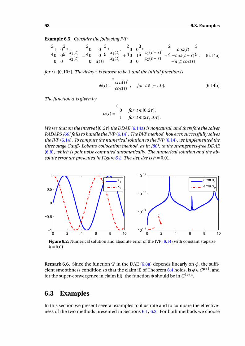
93 6.3. Examples
Example 6.5. Consider the following IVP1 00 00 0
[x1(t )x2(t )
]=0 0
0 00 α(t )
[x1(t )x2(t )
]+0 0
0 10 0
[x1(t −τ)x2(t −τ)
]+ cos(t )−cos(t −τ)−a(t )cos(t )
, (6.14a)
for t ∈ [0,10τ]. The delay τ is chosen to be 1 and the initial function is
φ(t ) =[
si n(t )cos(t )
], for t ∈ [−τ,0]. (6.14b)
The function α is given by
α(t ) =
0 for t ∈ [0,2τ],
1 for t ∈ (2τ,10τ].
We see that on the interval [0,2τ] the DDAE (6.14a) is noncausal, and therefore the solverRADAR5 [60] fails to handle the IVP (6.14). The BVP method, however, successfully solvesthe IVP (6.14). To compute the numerical solution to the IVP (6.14), we implemented thethree stage Gauß- Lobatto collocation method, as in [80], to the strangeness-free DDAE(6.8), which is pointwise computed automatically. The numerical solution and the ab-solute error are presented in Figure 6.2. The stepsize is h = 0.01.
0 2 4 6 8 10−1
−0.5
0
0.5
1
x1x2
0 2 4 6 8 1010−16
10−14
10−12
10−10
error x1error x2
Figure 6.2: Numerical solution and absolute error of the IVP (6.14) with constant stepsizeh = 0.01.
Remark 6.6. Since the function G in the DAE (6.8a) depends linearly on φ, the suffi-cient smoothness condition so that the claim ii) of Theorem 6.4 holds, is φ ∈Cµ+1, andfor the super-convergence in claim iii), the function φ should be in C 2s+µ.
6.3 Examples
In this section we present several examples to illustrate and to compare the effective-ness of the two methods presented in Sections 6.1, 6.2. For both methods we choose

6.3. Examples 94
the number of stages s is three. First we consider their performance for retarded andneutral DDAEs.
Example 6.7. Consider the DDAE[0 t0 0
][x1(t )x2(t )
]=[
1 00 1
][x1(t )x2(t )
]+[
0 10 0
][x1(t −τ)x2(t −τ)
]+[−e t +1
−t
], (6.15)
in the time interval I= [0,10τ], with the delay τ= 1. We choose an initial function φ to
be
[e t
t
]for t ∈ [−τ,0]. Taking the derivative of the second equation of (6.15) and scaling
it with t , we deduce that0 = t x2(t )− t .
Adding this equation to the first equation of (6.15) and eliminating t x2(t ) on both sides,we see that
0 = x1(t )+x2(t −τ)−e t +1− t .
Therefore, the strangeness-free formulation of the DDAE (6.15) is[0 00 0
]x(t ) =
[1 00 1
]x(t )+
[0 10 0
]x(t −τ)+
[−e t +1− t−t
],
which implies that (6.15) is of neutral type.
The relative errors with respect to the exact solution x(t ) =[
e t
t
]for the two methods are
presented in Figure 6.3. There, by GMOS (resp. BVP) we denote the relative errors ofthe solution obtained by the generalized method of steps (resp., the BVP method). Theconstant stepsize is h = 0.01.
In the next example we consider a causal DDAE of advanced type.
Example 6.8. Consider the DDAE[0 10 0
]x(t ) =
[1 00 1
]x(t )+
[1 00 1
]x(t −τ)+
[1−e t −e t−1
1−2t
], (6.16)
in the time interval I = [0,10τ], with the delay τ = 1. From (6.16), one obtains thestrangeness-free DDAE[
0 00 0
]x(t ) =
[1 00 1
]x(t )+
[1 00 1
]x(t −τ)+
[0 10 0
]x(t −τ)+
[−1−e t −e t−1
1−2t
],
which implies that (6.16) is of advanced type. The relative errors with respect to the
exact solution x(t ) =[
e t
t
]are also presented in Figure 6.3. There, by GMOS (resp. BVP)
we denote the relative errors of the solution obtained by the generalized method of steps(resp., the BVP method). The constant stepsize is h = 0.01.
In Figure 6.3, we see that if a DDAE is of retarded or neutral type, then the general-ized method of steps seems to be more efficient than the BVP method. Otherwise, if aDDAE is of advanced type then the BVP method seems to be a better candidate. The

95 6.3. Examples
0 2 4 6 8 1010−18
10−16
10−14
10−12
10−10
GMOSBVP
0 2 4 6 8 1010−16
10−14
10−12
10−10
10−8
GMOSBVP
Figure 6.3: Relative error of the DDAE (6.15) (left) and of the DDAE (6.16) (right) with con-stant stepsize h = 0.01.
reason is that the generalized method of steps solves the discretized system on consec-utive intervals and hence, due to the advancedness of a DDAE, the error on each inter-val [(i −1)τ, iτ] is rapidly amplified when one proceeds to the next interval [iτ, (i +1)τ].
Furthermore, the BVP method can also handle advanced DDAEs, whose the strangeness-free formulations are of high order. This is demonstrated in the following example.
Example 6.9. Consider the DDAE0 0 10 0 00 1 00 0 0
x1(t )
x2(t )x3(t )
=
0 1 00 0 10 0 0
H(t −τ) 0 0
x1(t )
x2(t )x3(t )
+
0 0 01 0 00 0 00 0 0
x1(t −τ)
x2(t −τ)x3(t −τ)
+
−t−1−e t−1
1−H(t −τ)e t
,
(6.17)on the time interval I= [0,`τ) with `= 6, τ= 1. Here H is the Heaviside function givenby
H(t ) =
0, if t 6 0,
1, if t > 0.
By directly verifying Hypothesis 5.22, one sees that the shift index of (6.17) is given by
κ=
1, if t 6 τ,
0, if t > τ.
By performing as in Example 5.8, we deduce that the regular, strangeness-free formula-tion of the DDAE (6.17) takes the form
−0 0 0
0 0 01 0 0
x1(t )x2(t )x3(t )
=0 1 0
0 0 10 0 0
x1(t )x2(t )x3(t )
+0 0 0
1 0 00 0 0
x1(t −τ)x2(t −τ)x3(t −τ)
+1 0 0
0 0 00 0 0
x1(t )x2(t )x3(t )
+−t −e t−1
−1−e t−1
−e t
, for t ∈ (0,τ),
(6.18a)

6.3. Examples 96
and 000
=0 1 0
0 0 11 0 0
x1(t )x2(t )x3(t )
+0 0 0
1 0 00 0 0
x1(t −τ)x2(t −τ)x3(t −τ)
+1 0 0
0 0 00 0 0
x1(t )x2(t )x3(t )
+−t −e t−1
−1−e t−1
−e t
, for t ∈ (τ,`τ),
(6.18b)
Unfortunately, the generalized method of steps fails to determine the strangeness-freeformulation (6.18), because it is not a first order DDAE. Furthermore, it is complicatedto implement Runge-Kutta methods or BDF methods for (6.18) and the error in the ap-proximation of x(t − τ) is also an important issue. For higher dimensional DDAEs, ifthe considered system is causal and of advanced type, then typically the strangeness-freeformulation can contain high order derivatives of x(t ) and x(t −τ), which makes it im-possible to use the generalized method of steps. The BVP method, however, can work finein this case, if the strangeness indexµ is sufficiently small. For example, the BVP methodsuccessfully handles the corresponding IVP for the DDAE (6.17), since the strangeness-index of the DAE (6.8a) is always two. The numerical solution and the relative errorare presented in Figure 6.4. Here we use again the three stage Gauß-Lobatto collocationmethod, as in [80], to the strangeness-free DDAE (6.9), which is pointwise computed au-tomatically. The constant stepsize is h = 0.01.
0 2 4 6 8 10−1
0
1
2
3
4
5
x1x2x3
0 2 4 6 8 1010−20
10−15
10−10
10−5
error x1error x2error x3
Figure 6.4: The solution and the absolute error of the DDAE (6.17) with constant stepsizeh = 0.01.

Chapter 7
Solvability Analysis of GeneralNonlinear DDAEs
This chapter is devoted to the solvability analysis of initial value problems for generalnonlinear DDAEs of the form
F (t , x(t ), x(t ), x(t −τ)) = 0, (7.1a)
for all t ∈ I= (0, t f ), together with an initial function
x(t ) =φ(t ), for all t ∈ [−τ,0]. (7.1b)
The extensions of the results in Chapters 5, 6 for general nonlinear, noncausal DDAEsare desired. However, this is still an open question and therefore, in this chapter weonly present some important results in prior investigations about the numerical anal-ysis of nonlinear DDAEs.
For notational convenience, we consider only real-valued problems where both F andx are real vector-valued functions. To obtain the results for complex-valued problems,we can analyze the real and imaginary part of the equation and the unknown sepa-rately. Furthermore, let us restrict our consideration to square systems, i. e., m = n.
Together with (7.1a), we are also interested in the associated DAE
F (t , x(t ), x(t )) = 0. (7.2)
In order to discuss the theoretical and numerical solution of the IVP (7.1), within thischapter we assume that the IVP (7.1) has a unique solution. Similar to the linear case,we see that the piecewise differentiable solution concept is more suitable for IVPs ofDDAEs. Therefore, we recall this concept in the following definition.
Definition 7.1. i) A function x : Iτ → Rn is called a piecewise differentiable solution of(7.1a), if it is continuous, piecewise continuously differentiable and satisfies (7.1a) al-most everywhere. Throughout this chapter whenever we speak of a solution, we meana piecewise differentiable solution.ii) An initial function φ is called consistent if the IVP (7.1) has at least one solution.iii) The DDAE (7.1a) is called solvable if it has at least one solution. It is called regu-
97

98
lar if in addition, the solution to the IVP (7.1) is unique, provided a consistent initialfunction.
There are very few references about the solvability analysis of nonlinear DDAEs andamong them we want to mention the following papers [5, 60, 68, 86] for solution pro-cedures, and [10] for some difficulties that may occur for the numerical integration ofDDAEs. Except [5], where the type of a DDAE is examined and the index reductionprocedure is performed whenever it is necessary, the other references directly applynumerical methods to a given DDAE, without any regularization procedure.
Precisely, the authors showed in [5] that a retarded, Hessenberg DDAE of differentia-tion index at most three, takes the following form
x(t ) = f (x(t ), x(t −τ), y(t ), y(t −τ)),0 = g (x(t ), x(t −τ), y(t )),
(7.3)
(where ∂g∂y is nonsingular) for differentiation index one,
x(t ) = f (x(t ), x(t −τ), y(t )),0 = g (x(t )),
(7.4)
(where ∂g∂x
∂ f∂y is nonsingular) for differentiation index two,
y(t ) = f (x(t ), x(t −τ), y(t ), y(t −τ), z(t )),x(t ) = g (x(t ), x(t −τ), y(t )),0 = h(x(t )),
(7.5)
(where ∂h∂x
∂g∂y
∂ f∂z is nonsingular) for differentiation index three.
Furthermore, in the cases that the function g in (7.3) is allowed to depend on y(t −τ)and g in (7.4) is allowed to depend on x(t − τ) then the corresponding system is ofneutral type. Then, in [5] the authors constructed an index reduction procedure toderive a delay-essential-underlying ODE (DEUODE) and investigated the convergenceand order of numerical methods like BDF methods, projected implicit Runge-Kuttamethods applied to index one and index two retarded and neutral Hessenberg DDAEs.It is also shown that a DDAE is (numerically) stable, or well-conditioned if its DEUODEis (numerically) stable.
Without considering any regularization or any index reduction procedure, in the article[60] the authors applied the 3-stage Radau IIA method and implemented it in the solverRADAR5 to compute the solution of IVPs for quasi-linear DDAEs of the form
M y(t ) = f (t , y(t ), y(α(t , y(t )))), (7.6a)
with the initial condition
y(t0) = y0, y(t ) = g (t ), for t < t0, (7.6b)
where the matrix M is constant but allowed to be singular. The state-dependent delayα(t , y(t )) satisfies α(t , y(t )) 6 t for all t ≥ t0. Note that this includes small delays, i.e.,

99
t −α(t , y(t )) ¿ t , and vanishing delays, i.e., α(t , y(t )) = t for some t .The Radau IIA method has successfully handled a variety of systems including retardedand neutral DDEs and also DDAEs where the associated non-delayed DAE is regularand strangeness-free. However, since no regularization procedure was considered forthe DDAE (7.6a), this method may not work, or it may give wrong results for generalhigh index, noncausal DDAEs.
The other important studies are [68, 86] where the authors considered retarded DDAEsin the semi-explicit form
x(t ) = f (t , x(t ), y(t ), x(α(t , x(t )))),0 = g (t , x(t ), y(t ), x(α(t , x(t )))),
(7.7)
(where ∂g∂y is nonsingular) for differentiation index one, and
x(t ) = f (t , x(t ), y(t ), x(α(t , x(t )))),0 = g (t , x(t )),
(7.8)
(where ∂g∂x
∂ f∂y is nonsingular) for differentiation index two.
Here the delay α(t , x(t )) is state-dependent and non-vanishing, i.e., there exist δ > 0such that α(t , x) 6 t −δ. There in [68], the author investigated the convergence of col-location methods for the system (7.7), (7.8). One important contribution of the studies[60, 68] is the discontinuity detection in the state dependent delay case.
We further note that all the investigation presented above, similar to the other in-vestigation about the solvability analysis of IVPs for linear DDAEs [25, 29, 83, 122, 142],are restricted to systems that have the following features:
i) The associated non-delayed DAE is uniquely solvable, and hence the consideredDDAE is causal;
ii) The considered DDAE is of either retarded or neutral type.Furthermore, prior work on DDAEs (for both linear and nonlinear systems) usuallymake use of the method of steps for the solution procedure. Because of this reason, wenow recall the method of steps for nonlinear, causal DDAEs.Introducing the vector-valued functions for each i ∈N
xi : [0,τ] → Rn
t 7→ x(t + (i −1)τ), (7.9a)
and
Fi : [0,τ]×Rn ×Rn ×Rn → Rn
(t , xi (t ), xi (t ), xi−1(t )) 7→ F (t + (i −1)τ, xi (t ), xi (t ), xi−1(t )), (7.9b)
we rewrite the IVP (7.1) as a sequence of DAEs
Fi (t , xi (t ), xi (t ), xi−1(t )) = 0, (7.10a)
for all t ∈ (0,τ), and for all i = 1, 2, . . . ,`. The function x0 is prescribed by

100
x0(t ) := φ(t −τ). Here equation (7.10a) is a parameter dependent DAE in variable xi
with a function parameter xi−1. The initial condition for the DAE (7.10a) is
xi (0) = xi−1(τ). (7.10b)
Assuming that the DDAE (7.1a) is causal, it implies that the IVP (7.10) is uniquely solv-able for any sufficiently smooth function parameter xi−1 and any consistent initial vec-tor xi (0). Having found the function xi , we can proceed in the same way to obtain xi+1
and so on. Therefore, the solution x(t ) to the IVP (7.1) is successfully constructed stepby step, provided that an initial function φ is sufficiently smooth and satisfies certainconsistency conditions.
In analogy to the linear DDAE case, we see that there are two unmentioned issuesin prior investigations that motivates our future research:
1. How to categorize general nonlinear, noncausal DDAEs by their types (retarded,neutral and advanced) and to solve IVPs for retarded and neutral systems.
2. How to classify advanced DDAEs in order to figure out which class of advancedDDAEs can be efficiently integrated.
Conclusion and Outlook
In this chapter we present some conclusions and some possible open problems foundduring the work.
Conclusion
The combination of differential-algebraic equations arising from an automatic model-ing based approach and the appearance of time delays due to the physical propertiesor feedback control naturally leads to delay differential-algebraic equations (DDAEs).Despite of their natural importance and broad range of applications, DDAEs are notwell understood even for fundamental problems such as the solvability analysis. Inthis thesis we have mainly studied the analytical and numerical solution to initial valueproblems for linear DDAEs.
Important properties inherited from the theories of DAEs and of DDEs lead to crit-ical consequences for DDAEs such as a solution concept, the discontinuity propaga-tion or a system classification. However, the combination between these two sub-classes DAEs and DDEs has lead to many interesting properties. In Chapter 3 we havediscussed some characteristics of DDAEs, which are the starting points for importantconsequences associated with the computational solution of the corresponding IVPs.In summary, initial value problems for DDAEs present four different difficulties:
1. The hidden type of a system, i. e., retarded, neutral or advanced.2. The causality or noncausality of a system.3. The linearity or nonlinearity of a system.4. The type of delays and the number of delays.
Different from prior studies, which mostly considered the last two difficulties, in thiswork we have considered the first two difficulties. Until now, there is no treatment forall these four difficulties.
Chapter 4 addresses linear time invariant DDAEs, where all the system coefficientsare constant matrices. The DDAEs are studied by three approaches: first, analyzingthe structure of matrix triples, second, a matrix polynomial approach, and third, an al-gebraic method. An important contribution of this chapter is to point out the link be-tween the existence and uniqueness of solutions (of IVPs for DDAEs) and the regularityof either the matrix pair (E , A) or the matrix triple (E , A,B), depending on whether thetime interval is bounded or not. This result allows to study the solvability of a DDAEby investigating spectral properties of its matrix coefficients. Furthermore, the ma-
101

102
trix polynomial approach is applicable for a much broader class of time delay systemsincluding both underdetermined and overdetermined systems. Finally, another ap-proach in the theory of DAEs, namely an algebraic method, is examined to study gen-eral noncausal DDAEs of retarded and neutral types.
Chapter 5 studies the solvability analysis and reformulation of general linear timevariable coefficients DDAEs, with a special focus on the numerical solution. IVPs forDDAEs are studied by two different approaches, which aim at different types of DDAEs.While the first approach, the generalized method of steps, can successfully handle re-tarded and neutral DDAEs, the second one, the BVP method, is advantageous for study-ing advanced DDAEs.The first approach, by introducing the shift index concept in order to estimate thenoncausality of a DDAE, has extended the results in the theory of DAEs [75] to de-duce a strangeness-free formulation (and consequently, the underlying DDE), and alsoto obtain the necessary and sufficient conditions for a consistent initial function anda consistent inhomogeneity. To compute the solution of IVPs for DDAEs, numericalmethods for DDEs are applied to the strangeness-free formulation, which is pointwisecomputed automatically. Furthermore, the nonadvancedness of a considered DDAE ischecked by a verifiable condition.Different from the first approach, the second approach removes the delay and studiesIVPs for DDAEs as BVPs for DAEs. Thus, one does not need to worry about the delayand the type of the system. The interesting feature of this approach is that it is not be-ing limited to retarded and neutral DDAEs but clearly shows which advanced DDAEs(and consequently, advanced DDEs) can be efficiently integrated. This concept has notyet been mentioned in the literature, even for advanced DDEs.
Based on the two methods presented in Chapter 5, we have developed in Chap-ter 6 two strategies for the numerical integration of general linear DDAEs. The firststrategy is based on the observation that the generalized method of steps is applica-ble for retarded and neutral DDAEs. As discussed in Chapter 5, the strangeness-freeformulation is pointwise computed in parallel with verifying the type of the consid-ered system to prevent the advanced situation. Following the method of steps, theRadau collocation method with Lagrange interpolation for the history function is thenapplied to this strangeness-free formulation. On the other hand, the second strategymakes use of well-known integration methods for the corresponding boundary valueproblems of the reformulated DAEs. The Gauß-Lobatto collocation method is appliedto the strangeness-free formulation of the reformulated DAEs. It turns out that, fordifferent type of DDAEs, one should choose different integration strategies. In moredetails, the generalized method of steps has shown better performance for retarded orneutral DDAEs, while the BVP method is more suitable for advanced DDAEs. The BVPmethod has shown the possibility to treat not only causal, advanced DDAEs but evennoncausal, advanced DDAEs, whose the strangeness-free formulation is of high orderand has complicated structure.

103
Outlook
There are many possible open research problems related to the work in this thesis. Inthe following, we list some related open problems and research directions, which maybe of interest in the future.
Regularization and numerical solution to general nonlinear DDAEs. Linear DDAEsare treated within the scope of this thesis. However, most problems in real life appli-cations are nonlinear and therefore, a systematic study for nonlinear DDAEs is indis-pensable. Nevertheless, only two special classes of causal systems, namely Hessenbergsystems ([5]) and semi-explicit, index one systems ([10], [60]) have been studied. Thecases of advanced DDAEs and general noncausal DDAEs are still entirely open. Weexpect that the two approaches presented in Chapter 5 can be extended to generalnonlinear DDAEs.
Regularization of delay descriptor systems. DDAEs with control variable are oftencalled delay descriptor systems, which naturally occurs in many applications. Besidesthe two approaches presented in Chapter 5, it would be interesting to extend the be-havior approach ([76]) to delay descriptor systems.
Fundamental control properties of delay descriptor systems. Once the regulariza-tion are well studied for delay descriptor systems, we wish to investigate fundamentalcontrol concepts such as stability, stabilization, controllability, observability, etc. Alsoof interest is the spectral analysis of Delay-DAEs and the computation of spectral ex-ponents and spectral intervals.

104

Bibliography
[1] R. M. ALEXANDER, Simple models of human movement, Appl. Mech. Rev., (1995),pp. 461 – 469. (Cited on page 5.)
[2] P. ANTOGNETTI AND G. MASSOBRIO, Semiconductor device modeling with SPICE,McGraw-Hill, New York, NY, 1997. (Cited on page 2.)
[3] C. ARÉVALO AND P. LÖTSTEDT, Improving the accuracy of BDF methods for index 3differential-algebraic equations, BIT, 35 (1995), pp. 297–308. (Cited on page 21.)
[4] U. M. ASCHER, R. MATTHEIJ, AND R. RUSSELL, Numerical Solution of Bound-ary Value Problems for Ordinary Differential Equations, SIAM Publications,Philadelphia, PA, 2nd ed., 1995. (Cited on pages 81 and 91.)
[5] U. M. ASCHER AND L. R. PETZOLD, The numerical solution of delay-differentialalgebraic equations of retarded and neutral type, SIAM J. Numer. Anal., 32 (1995),pp. 1635–1657. (Cited on pages 2, 3, 32, 34, 98, and 103.)
[6] , Computer Methods for Ordinary Differential and Differential-AlgebraicEquations, SIAM Publications, Philadelphia, PA, 1998. (Cited on pages 2, 19,and 21.)
[7] S. BÄCHLE AND F. EBERT, Element-based topological index reduction fordifferential-algebraic equations in circuit simulation, Technical Report 246, DFGResearch Center MATHEON, TU Berlin, Berlin, Germany, 2004. Submitted forpatenting. (Cited on page 7.)
[8] Z. BAI, D. BINDEL, J. CLARK, J. C. Z, J. DEMMEL, N. ZHOU, K. PISTER, AND N. Z.Z, New numerical techniques and tools in SUGAR for 3D MEMS Simulation, inProc. Fourth Technical International Conference on Modeling and Simulation ofMicrosystems, Hilton Head Island, SC, 2001, pp. 31–34. (Cited on page 21.)
[9] Z. BAI, P. DE WILDE, AND R. W. FREUND, Reduced order modeling, in Hand-book of Numerical Analysis. Vol. XIII, Numerical Methods in Electromagnetics,W. Schilders and E. J. W. ter Maten, eds., 2005, pp. 825–895. (Cited on page 21.)
[10] C. T. H. BAKER, C. A. H. PAUL, AND H. TIAN, Differential algebraic equationswith after-effect, J. Comput. Appl. Math., 140 (2002), pp. 63–80. (Cited on pages 2,3, 32, 98, and 103.)
105

BIBLIOGRAPHY 106
[11] M. BANDYOPADHYAY AND S. BANERJEE, A stage-structured prey - predator modelwith discrete time delay, Appl. Math. Comput., 182 (2006), pp. 1385 – 1398. (Citedon page 2.)
[12] A. BELLEN, N. GUGLIELMI, AND A. RUEHLI, Methods for linear systems of circuitdelay differential equations of neutral type, IEEE Trans. Circ. and Syst., 46 (1999),pp. 212–215. (Cited on page 8.)
[13] A. BELLEN AND M. ZENNARO, Numerical Methods for Delay Differential Equa-tions, Oxford University Press, Oxford, UK, 2003. (Cited on pages 24, 25, 26,and 87.)
[14] R. BELLMAN, On the computational solution of differential-difference equations,J. Math. Anal. Appl., 2 (1961), pp. 108 – 110. (Cited on page 26.)
[15] R. BELLMAN AND K. L. COOKE, Differential-difference equations, Mathematics inScience and Engineering, Elsevier Science, 1963. (Cited on pages 2, 24, 25, 26,and 38.)
[16] , On the computational solution of a class of functional differential equa-tions, J. Math. Anal. Appl., 12 (1965), pp. 495 – 500. (Cited on page 26.)
[17] R. E. BELLMAN, J. D. BUELL, AND R. E. KALABA, Numerical integration of adifferential-difference equation with a decreasing time-lag, Commun. ACM, 8(1965), pp. 227–228. (Cited on page 26.)
[18] L. T. BIEGLER, S. L. CAMPBELL, AND V. MEHRMANN, eds., Control and Opti-mization with Differential-Algebraic Constraints, SIAM Publications, Philadel-phia, PA, 2012. (Cited on page 2.)
[19] S. BOISGÉRAULT, Growth bound of delay-differential algebraic equations,Comptes Rendus Mathematique, 351 (2013), pp. 645 – 648. (Cited on page 2.)
[20] L. BOLTZMAN, Zur Theorie der elastischen Nachwirkungen, Leipzig: Verlag Jo-hann Ambrosius Barth, 1909, pp. 616–644. (Cited on page 2.)
[21] R. BRAYTON, Small-signal stability criterion for electrical networks containinglossless transmission lines, IBM J. RES. DEV., 12 (1968), pp. 431–440. (Cited onpage 8.)
[22] K. E. BRENAN, S. L. CAMPBELL, AND L. R. PETZOLD, Numerical Solution ofInitial-Value Problems in Differential Algebraic Equations, SIAM Publications,Philadelphia, PA, 2nd ed., 1996. (Cited on pages 2, 19, and 21.)
[23] R. BYERS, T. GEERTS, AND V. MEHRMANN, Descriptor systems without controlla-bility at infinity, SIAM J. Cont., 35 (1997), pp. 462–479. (Cited on page 56.)
[24] R. BYERS, P. KUNKEL, AND V. MEHRMANN, Regularization of linear descriptor sys-tems with variable coefficients, SIAM J. Cont., 35 (1997), pp. 117–133. (Cited onpage 56.)

107 BIBLIOGRAPHY
[25] S. L. CAMPBELL, Singular linear systems of differential equations with delays,Appl. Anal., 2 (1980), pp. 129–136. (Cited on pages 2, 3, 32, 35, 43, and 99.)
[26] , Singular Systems of Differential Equations I, Pitman, San Francisco, CA,1980. (Cited on pages 11, 13, and 43.)
[27] , Index two linear time varying singular systems of differential equations,Circ. Syst. Signal Process., 5 (1986), pp. 97–108. (Cited on page 74.)
[28] , A general form for solvable linear time varying singular systems of differen-tial equations, SIAM J. Math. Anal., 18 (1987), pp. 1101–1115. (Cited on page 74.)
[29] , Comments on 2-D descriptor systems, Automatica, 27 (1991), pp. 189–192.(Cited on pages 2, 3, 32, and 99.)
[30] , Nonregular 2D descriptor delay systems, IMA J. Math. Control Appl., 12(1995), pp. 57–67. (Cited on pages 48 and 49.)
[31] S. L. CAMPBELL AND V. H. LINH, Stability criteria for differential-algebraic equa-tions with multiple delays and their numerical solutions, Appl. Math Comput.,208 (2009), pp. 397 – 415. (Cited on pages 2, 32, 34, 35, and 48.)
[32] S. L. CAMPBELL AND W. MARSZALEK, DAEs arising from traveling wave solutionsof PDEs, J. Comput. Appl. Math., 82 (1997), pp. 41 – 58. 7th ICCAM 96 Congress.(Cited on page 21.)
[33] S. L. CAMPBELL, C. D. MEYER, AND N. J. ROSE, Applications of the Drazin in-verse to linear systems of differential equations with singular constant coefficients,SIAM J. Appl. Math., 31 (1976), pp. 411–425. (Cited on page 12.)
[34] T. CARABALLO AND J. REAL, Navier-Stokes equations with delays, Proc. R. Soc. A,457 (2001), pp. 2441–2453. (Cited on page 9.)
[35] K. F. CHEN, Standing human - an inverted pendulum, Lat. Am. J. Phys. Educ.,(2008), pp. 197 – 200. (Cited on page 5.)
[36] H. CHI, J. BELL, AND B. HASSARD, Numerical solution of a nonlinear advance-delay-differential equation from nerve conduction theory, J. Math. Biol., 24(1986), pp. 583–601. (Cited on page 27.)
[37] E. N. CHUKWU, Stability and time-optimal control of hereditary systems, Mathe-matics in Science and Engineering, Elsevier Science, 1992. (Cited on page 2.)
[38] L. DAI, Singular Control Systems, Springer-Verlag, Berlin, Germany, 1989. (Citedon page 11.)
[39] L. DIECI AND T. EIROLA, On smooth decompositions of matrices, SIAM J. Matr.Anal. Appl., 20 (1999), pp. 800–819. (Cited on page 16.)
[40] R. DRIVER, Ordinary and delay differential equations, Applied mathematical sci-ences, Springer-Verlag, 1977. (Cited on pages 2 and 27.)

BIBLIOGRAPHY 108
[41] N. H. DU, V. H. LINH, V. MEHRMANN, AND D. D. THUAN, Stability and robuststability of linear time-invariant delay differential-algebraic equations., SIAM J.Matr. Anal. Appl., 34 (2013), pp. 1631–1654. (Cited on page 2.)
[42] DYNASIM AB, Dymola, Multi-Engineering Modelling and Simulation, Ideon Re-search Park - SE-223 70 Lund - Sweden, 2006. (Cited on page 2.)
[43] E. EICH-SOELLNER AND C. FÜHRER, Numerical Methods in Multibody Dynamics,European Consortium for Mathematics in Industry, Teubner, 1998. (Cited onpage 21.)
[44] , Numerical Methods in Multibody Dynamics, European Consortium forMathematics in Industry, Morgan Kaufmann, 2013. (Cited on page 6.)
[45] R. ENGLAND, R. LAMOUR, AND J. LOPEZ-ESTRADA, Multiple shooting using a di-chotomically stable integrator for solving DAEs, Appl. Numer. Math., 42 (2003),pp. 117–131. (Cited on page 91.)
[46] T. ERNEUX, Applied Delay Differential Equations, Surveys and Tutorials in theApplied Mathematical Sciences, Springer, 2009. (Cited on pages 2 and 27.)
[47] D. ESTÉVEZ-SCHWARZ, U. FELDMANN, R. MÄRZ, S. STURTZEL, AND C. TISCHEN-DORF, Finding beneficial DAE structures in circuit simulation, Tech. Report 00-7,Institut für Mathematik, Humboldt Universität zu Berlin, Berlin, Germany, 2000.(Cited on page 7.)
[48] D. ESTÉVEZ-SCHWARZ AND C. TISCHENDORF, Structural analysis for electricalcircuits and consequences for MNA, Internat. J. Circ. Theor. Appl., 28 (2000),pp. 131–162. (Cited on page 7.)
[49] B. FABIEN, Analytical System Dynamics: Modeling and Simulation, Springer,2008. (Cited on page 2.)
[50] M. J. GARRIDO-ATIENZA AND P. MARÍN-RUBIO, Navier-Stokes equations with de-lays on unbounded domains, Nonlinear Anal., 64 (2006), pp. 1100–1118. (Citedon page 9.)
[51] C. W. GEAR, The simultaneous numerical solution of differential-algebraic equa-tions, IEEE Trans. Circ. Theor., CT-18 (1971), pp. 89–95. (Cited on page 1.)
[52] M. GERDTS, Direct shooting method for the numerical solution of higher indexDAE optimal control problems, J. Optim. Th. Appl., 117 (2003), pp. 267–294.(Cited on page 91.)
[53] , Local minimum principle for optimal control problems subject todifferential-algebraic equations of index two, J. Optim. Th. Appl., 130 (2006),pp. 443–462. (Cited on page 21.)
[54] H. GLUESING-LUERSSEN, Linear Delay-Differential Systems with CommensurateDelays: An Algebraic Approach, Springer, Berlin, 2002. (Cited on pages 24 and 25.)
109 BIBLIOGRAPHY
[55] I. GOHBERG, P. LANCASTER, AND L. RODMAN, Matrix Polynomials, AcademicPress, New York, NY, 1982. (Cited on page 55.)
[56] K. GOPALSAMY, Stability and Oscillations in Delay Differential Equations of Pop-ulation Dynamics, Mathematics and Its Applications, Springer, 1992. (Cited onpages 2 and 27.)
[57] C. GROSSMANN, H. ROOS, AND M. STYNES, Numerical Treatment of Partial Dif-ferential Equations, Springer-Verlag Berlin Heidelberg, 2007. (Cited on page 9.)
[58] K. GU AND S.-I. NICULESCU, Survey on recent results in the stability and controlof time-delay systems, J. Dyn. Sys., Meas., Control, 125(2) (2003), pp. 158–165.(Cited on page 2.)
[59] N. GUGLIELMI AND E. HAIRER, Implementing Radau IIA methods for stiff delaydifferential equations, Computing, 67 (2001), pp. 1–12. (Cited on page 88.)
[60] , Computing breaking points in implicit delay differential equations, Adv.Comput. Math., 29 (2008), pp. 229–247. (Cited on pages vi, viii, 2, 3, 32, 34, 35,87, 88, 89, 93, 98, 99, and 103.)
[61] A. W. GULIN, O. M. DROSDOVA, S. W. KARTYSHOV, AND I. M. KOSHELEV, Numer-ical analysis of stability of high-order differential algebraic systems with delays,tech. report, Keldysh Institute of Applied Mathematics, Soviet Academy of Sci-ences, Moscow, RU, 1988. (Cited on page 2.)
[62] M. GÜNTHER AND U. FELDMANN, CAD-based electric-circuit modeling in indus-try I. Mathematical structure and index of network equations, Surv. Math. Ind., 8(1999), pp. 97–129. (Cited on page 7.)
[63] P. HA AND V. MEHRMANN, Analysis and reformulation of linear delay differential-algebraic equations, Electr. J. Lin. Alg., 23 (2012), pp. 703–730. (Cited on pages ix,xi, 2, 22, 35, and 37.)
[64] P. HA AND V. MEHRMANN, Analysis and numerical solution of linear delaydifferential-algebraic equations, in prepatation, Institut für Mathematik, TUBerlin, D-10623 Berlin, 2014. (Cited on page xi.)
[65] P. HA, V. MEHRMANN, AND A. STEINBRECHER, Analysis of linear variable coef-ficient delay differential-algebraic equations, J. Dynam. Differential Equations,(2014), pp. 1–26. (Cited on pages ix, xi, 2, 3, 35, 37, and 68.)
[66] E. HAIRER, C. LUBICH, AND M. ROCHE, The Numerical Solution of Differential-Algebraic Systems by Runge-Kutta Methods, Springer-Verlag, Berlin, Germany,1989. (Cited on page 19.)
[67] J. HALE AND S. LUNEL, Introduction to Functional Differential Equations,Springer, 1993. (Cited on page 25.)
[68] R. HAUBER, Numerical treatment of retarded differential algebraic equations bycollocation methods, Adv. Comput. Math., 7 (1997), pp. 573–592. (Cited onpages 32, 34, 89, 98, and 99.)

BIBLIOGRAPHY 110
[69] C.-W. HO, A. RUEHLI, AND P. A. BRENNAN, The modified nodal approach to net-work analysis, IEEE Trans. Circ. and Syst., 22 (1975), pp. 504–509. (Cited onpage 7.)
[70] R. HORN AND C. JOHNSON, Matrix Analysis, Cambridge University Press, 1990.(Cited on page 50.)
[71] P. HÖVEL AND E. SCHÖLL, Control of unstable steady states by time-delayed feed-back methods, Phys. Rev. E, 72 (2005), p. 046203. (Cited on page 2.)
[72] A. ILCHMANN AND T. REIS, Surveys in Differential-Algebraic Equations I,Differential-Algebraic Equations Forum, Springer, 2013. (Cited on page 2.)
[73] T. INSPERGER, R. WOHLFART, J. TURI, AND G. STEPAN, Equations with advancedarguments in stick balancing models, vol. 423 of Lecture Notes in Control andInformation Sciences, Springer Berlin Heidelberg, 2012, pp. 161–172. (Cited onpage 27.)
[74] Y. KUANG, Delay Differential Equations: With Applications in Population Dy-namics, Mathematics in Science and Engineering, Elsevier Science, 1993. (Citedon pages 2, 27, and 32.)
[75] P. KUNKEL AND V. MEHRMANN, Differential-Algebraic Equations – Analysis andNumerical Solution, EMS Publishing House, Zürich, Switzerland, 2006. (Citedon pages 2, 3, 13, 14, 15, 18, 21, 22, 33, 43, 67, 81, 91, and 102.)
[76] P. KUNKEL, V. MEHRMANN, AND W. RATH, Analysis and numerical solution ofcontrol problems in descriptor form, Math. Control, Signals, Sys., 14 (2001),pp. 29–61. (Cited on pages 67 and 103.)
[77] P. KUNKEL, V. MEHRMANN, W. RATH, AND J. WEICKERT, A new software pack-age for linear differential–algebraic equations, SIAM J. Sci. Comput., 18 (1997),pp. 115–138. (Cited on page 91.)
[78] P. KUNKEL, V. MEHRMANN, AND R. STÖVER, Multiple shooting for unstructurednonlinear differential-algebraic equations of arbitrary index, SIAM J. Numer.Anal., 42 (2004), pp. 2277–2297. (Cited on page 91.)
[79] , Symmetric collocation for unstructured nonlinear differential-algebraicequations of arbitrary index, Numer. Math., 98 (2004), pp. 277–304. (Cited onpages 4 and 91.)
[80] P. KUNKEL AND R. STÖVER, Symmetric collocation methods for linear differential-algebraic boundary value problems, Numer. Math., 91 (2002), pp. 475–501. (Citedon pages 4, 91, 92, 93, and 96.)
[81] R. LAMOUR, A shooting method for fully implicit index-2 DAEs, SIAM J. Sci. Com-put., 18 (1997), pp. 94–114. (Cited on page 91.)
[82] R. LAMOUR, R. MÄRZ, AND C. TISCHENDORF, Differential-algebraic equations:A projector based analysis., Differential-Algebraic Equations Forum 1. Berlin:Springer, 2013. (Cited on pages 2, 7, and 19.)
111 BIBLIOGRAPHY
[83] Y. LI, L. SUN, AND Q. YU, Stability of two-step Runge - Kutta methods for neu-tral delay differential-algebraic equations, Internat. J. Comput. Math., 88 (2011),pp. 375–383. (Cited on pages 2, 3, 32, 34, and 99.)
[84] C. LIU, Q. ZHANG, AND X. DUAN, Dynamical behavior in a harvested differential-algebraic prey - predator model with discrete time delay and stage structure, J.Franklin Inst., 346 (2009), pp. 1038 – 1059. (Cited on page 2.)
[85] W. LIU, Asymptotic behavior of solutions of time-delayed Burgers’ equation, Dis-crete. Cont. Dyn.-B, 2 (2002), pp. 47–56. (Cited on page 8.)
[86] Y. LIU, Runge - Kutta collocation methods for systems of functional differentialand functional equations, Adv. Comput. Math., 11 (1999), pp. 315–329. (Cited onpages 34, 98, and 99.)
[87] I. D. LORAM, S. M. KELLY, AND M. LAKIE, Human balancing of an inverted pen-dulum: is sway size controlled by ankle impedance?, J. Physiol. (London), (2001),pp. 879 – 891. (Cited on page 6.)
[88] S. LORD, C. SHERRINGTON, H. MENZ, AND J. CLOSE, Falls in Older People: RiskFactors and Strategies for Prevention, Cambridge University Press, 2007. (Citedon page 4.)
[89] W. MARSZALEK AND S. CAMPBELL, DAEs arising from traveling wave solutions ofPDEs II, Comput. Math. Appl., 37 (1999), pp. 15 – 34. (Cited on page 21.)
[90] R. MÄRZ, On difference and shooting methods for boundary value problems indifferential-algebraic equations, Preprint 24, Sektion Mathematik, Humboldt-Universität zu Berlin, Berlin, Germany, 1982. (Cited on page 91.)
[91] THE MATHWORKS, INC., MATLAB Version 8.3.0.532 (R2014a), Natick, MA, 2014.(Cited on pages 2 and 76.)
[92] , Simulink Version 8.3, Natick, MA, 2014. (Cited on page 2.)
[93] V. MEHRMANN AND C. SHI, Transformation of high order linear differential-algebraic systems to first order, Numer. Alg., 42 (2006), pp. 281–307. (Cited onpages 21 and 22.)
[94] W. MICHIELS, Spectrum-based stability analysis and stabilisation of systems de-scribed by delay differential algebraic equations, IET Control Theory Appl., 5(2011), pp. 1829–1842. (Cited on page 2.)
[95] W. MICHIELS AND S.-I. NICULESCU, Stability and Stabilization of Time-DelaySystems: An Eigenvalue-based Approach, SIAM, 2007. (Cited on pages 2, 24, 26,and 27.)
[96] J. MILTON, J. L. CABRERA, T. OHIRA, S. TAJIMA, Y. TONOSAKI, C. W. EURICH,AND S. A. CAMPBELL, The time-delayed inverted pendulum: Implications for hu-man balance control, Chaos: An Interdisciplinary Journal of Nonlinear Science,19 (2009), p. 026110. (Cited on pages 4 and 6.)

BIBLIOGRAPHY 112
[97] N. MINORSKY, Nonlinear oscillations, Van Nostrand, 1962. (Cited on pages xv, 2,and 7.)
[98] P. G. MORASSO AND M. SCHIEPPATI, Can muscle stiffness alone stabilize uprightstanding?, J. Neurophysiol., (1999), pp. 1622 – 1626. (Cited on page 6.)
[99] P. MÜLLER, P. RENTROP, W. KORTÜM, AND C. FÜHRER, Constrained mechanicalsystems in descriptor form - identification, simulation and control, in Proceed-ings of Advanced Multibody System Dynamics in Stuttgart 1993, Kluwer 1993,pp. 451–456. 23.01.2007. (Cited on page 21.)
[100] H. NAKAJIMA, On analytical properties of delayed feedback control of chaos, Phys.Lett. A, 232 (1997), pp. 207 – 210. (Cited on page 2.)
[101] A. OPPENHEIM, A. WILLSKY, AND S. NAWAB, Signals and Systems, Prentice-Hallsignal processing series, Prentice Hall, 1997. (Cited on page 32.)
[102] M. OTTER, H. ELMQVIST, AND S. E. MATTSSON, Multidomain Modeling withModelica. Handbook of Dynamic System Modelling, Chapman & Hall/CRC, 2007,ch. 36. (Cited on page 21.)
[103] M. G. PANDY, Simple and complex models for studying function in walking, Phil.Trans. R. Soc. Lond. B, (2003), pp. 1501 – 1509. (Cited on page 5.)
[104] G. PLANAS AND E. HERNÁNDEZ, Asymptotic behaviour of two-dimensional time-delayed Navier-Stokes equations, Discrete. Contin. Dyn. S, 21 (2008), pp. 1245–1258. (Cited on page 8.)
[105] L. POPPE, The strangeness index of a linear delay differential-algebraic equationof retarded type, Proceedings of the Sixth IFAC Workshop on Time-Delay Sys-tems, 2006. (Cited on page 2.)
[106] D. PRAVICA, N. RANDRIAMPIRY, AND M. SPURR, Applications of an advanceddifferential equation in the study of wavelets, Appl. Comput. Harmon. Anal., 27(2009), pp. 2 – 11. (Cited on page 27.)
[107] K. PYRAGAS, Continuous control of chaos by self-controlling feedback, Phys. Lett.A, 170 (1992), pp. 421 – 428. (Cited on page 2.)
[108] P. RABIER AND W. RHEINBOLDT, Nonholonomic Motion of Rigid Mechanical Sys-tems from a DAE Viewpoint, SIAM Publications, 2000. (Cited on page 21.)
[109] G. RANGAIAH, Multi-objective Optimization: Techniques and Applications inChemical Engineering, Advances in process systems engineering, Hackensack,N.J., 2009. (Cited on pages xv and 9.)
[110] R. RIAZA, Differential-algebraic systems. Analytical aspects and circuit applica-tions, World Scientific Publishing Co. Pte. Ltd., Hackensack, NJ., 2008. (Cited onpages 2 and 7.)
[111] J.-P. RICHARD, Time-delay systems: an overview of some recent advances andopen problems, Automatica, 39 (2003), pp. 1667 – 1694. (Cited on pages 2 and 24.)

113 BIBLIOGRAPHY
[112] R. E. ROBERSON AND R. SCHWERTASSEK, Dynamics of Multibody Systems,Springer-Verlag, Heidelberg, Germany, 1988. (Cited on page 6.)
[113] D. ROSS, Controller design for time lag systems via a quadratic criterion, IEEETrans. Automat. Control, 16 (1971), pp. 664–672. (Cited on pages 9 and 10.)
[114] A. RUEHLI, Equivalent circuit models for three-dimensional multiconductor sys-tems, IEEE Trans. Microw. Theory Techn., 22 (1974), pp. 216–221. (Cited onpage 8.)
[115] , Partial element equivalent circuit (PEEC) method and its application in thefrequency and time domain, in Electromagnetic Compatibility, 1996. SymposiumRecord. IEEE 1996 International Symposium on, Aug 1996, pp. 128–133. (Citedon page 8.)
[116] A. RUEHLI, U. MIEKKALA, A. BELLEN, AND H. HEEB, Stable time domain solu-tions for EMC problems using PEEC circuit models, in Electromagnetic Compat-ibility, 1994. Symposium Record. Compatibility in the Loop., IEEE InternationalSymposium on, Aug 1994, pp. 371–376. (Cited on page 8.)
[117] J. SAND, On implicit Euler for high-order high-index DAEs, Appl. Numer. Math.,42 (2002), pp. 411 – 424. (Cited on page 21.)
[118] W. SCHIEHLEN, Multibody Systems Handbook, Springer-Verlag, Heidelberg, Ger-many, 1990. (Cited on page 6.)
[119] , Advanced multibody system dynamics, Kluwer Academic Publishers,Stuttgart, Germany, 1993. (Cited on page 6.)
[120] G. M. SCHOEN, Stability and Stabilization of Time-Delay Systems, phd thesis,Swiss federal institute of technology Zurich, Zurich, Switzerland, 1995. (Cited onpages xv, 9, 25, and 39.)
[121] V. SCHULZ, H. G. BOCK, AND M. C. STEINBACH, Exploiting invariants in the nu-merical solution of multipoint boundary value problems for DAE, SIAM J. Sci.Comput., 19 (1998), pp. 440–446. (Cited on page 91.)
[122] L. F. SHAMPINE AND P. GAHINET, Delay-differential-algebraic equations in con-trol theory, Appl. Numer. Math., 56 (2006), pp. 574–588. (Cited on pages 2, 3, 32,34, and 99.)
[123] C. SHI, Linear Differential-Algebraic Equations of Higher-Order and the Regular-ity or Singularity of Matrix Polynomial, dissertation, Institut für Mathematik, TUBerlin, Berlin, Germany, 2004. (Cited on pages 21 and 22.)
[124] B. SIMEON, Computational Flexible Multibody Dynamics: A Differential-Algebraic Approach, Differential-Algebraic Equations Forum, Springer, 2013.(Cited on page 6.)
[125] R. SIPAHI, S.-I. NICULESCU, C. ABDALLAH, W. MICHIELS, AND K. GU, Stabilityand stabilization of systems with time delay, Control Systems, IEEE, 31 (2011),pp. 38–65. (Cited on page 2.)
BIBLIOGRAPHY 114
[126] R. SIPAHI, T. VYHLÍDAL, S. NICULESCU, AND P. PEPE, Time Delay Systems: Meth-ods, Applications and New Trends, Lecture Notes in Control and Information Sci-ences, Springer, 2012. (Cited on pages 2 and 27.)
[127] A. STEINBRECHER, Numerical Solution of Quasi-Linear Differential-AlgebraicEquations and Industrial Simulation of Multibody Systems, dissertation, Institutfür Mathematik, TU Berlin, Berlin, Germany, 2006. (Cited on pages 3 and 6.)
[128] G. STÉPÁN AND L. KOLLÁR, Balancing with reflex delay, Math. Comput. Mod-elling, 31 (2000), pp. 199 – 205. Proceedings of the Conference on DynamicalSystems in Biology and Medicine. (Cited on page 6.)
[129] R. STÖVER, Numerische Lösung von linearen differential-algebraischen Randw-ertproblemen, dissertation, Fachbereich Mathematik, Universität Bremen, Bre-men, Germany, 1999. (Cited on page 81.)
[130] , Collocation methods for solving linear differential-algebraic boundaryvalue problems, Numer. Math., 88 (2001), pp. 771–795. (Cited on pages 4, 84,and 91.)
[131] H. TIAN, Q. YU, AND J. KUANG, Asymptotic stability of linear neutral de-lay differential-algebraic equations and Runge–Kutta methods, SIAM J. Numer.Anal., 52 (2014), pp. 68–82. (Cited on pages 2, 3, 32, and 34.)
[132] C. TISCHENDORF, Topological index calculation of differential-algebraic equa-tions in circuit simulation, Surv. Math. Ind., 8 (1999), pp. 187–199. (Cited onpage 7.)
[133] T. TUMA AND Á. BURMEN, Circuit Simulation with SPICE OPUS: Theoryand Practice, Modeling and simulation in science, engineering & technology,Springer London, 2009. (Cited on pages 2 and 7.)
[134] T. VYHLÍDAL, J. LAFAY, AND R. SIPAHI, Delay Systems: From Theory to Numer-ics and Applications, Advances in Delays and Dynamics, Springer InternationalPublishing, 2013. (Cited on pages 2 and 27.)
[135] T. J. WILLIAMS AND R. E. OTTO, A generalized chemical processing model forthe investigation of computer control, American Institute of Electrical Engineers,Part I: Communication and Electronics, Transactions of the, 79 (1960), pp. 458–473. (Cited on pages 9 and 10.)
[136] D. WINTER, Biomechanics and Motor Control of Human Movement, Wiley, 2009.(Cited on page 6.)
[137] D. A. WINTER, A. E. PATLA, F. PRINCE, M. ISHAC, AND K. GIELO-PERCZAK, Stiff-ness control of balance in quiet standing, J. Neurophysiol., (1998), pp. 1211 – 1221.(Cited on page 6.)
[138] M. H. WOOLLACOTT, C. VON HOSTEN, AND B. RÖSBLAD, Relation between muscleresponse onset and body segmental movements during postural perturbations inhumans, Exp. Brain Res., 72 (1988), pp. 593 – 604. (Cited on page 6.)

115 BIBLIOGRAPHY
[139] L. WUNDERLICH, Numerical treatment of second order differential-algebraic sys-tems, in Proc. Appl. Math. and Mech. (GAMM 2006, Berlin, March 27-31, 2006),vol. 6 (1), 2006, pp. 775–776. (Cited on pages 21 and 22.)
[140] , Analysis and Numerical Solution of Structured and Switched Differential-Algebraic Systems, dissertation, Institut für Mathematik, TU Berlin, Berlin, Ger-many, 2008. (Cited on page 22.)
[141] S. YANCHUK, M. WOLFRUM, P. HÖVEL, AND E. SCHÖLL, Control of unstablesteady states by long delay feedback, Phys. Rev. E, 74 (2006), p. 026201. (Citedon page 2.)
[142] W. ZHU AND L. R. PETZOLD, Asymptotic stability of linear delay differential-algebraic equations and numerical methods, Appl. Numer. Math., 24 (1997),pp. 247 – 264. (Cited on pages 2, 3, 32, 34, and 99.)
[143] , Asymptotic stability of Hessenberg delay differential-algebraic equations ofretarded or neutral type, Appl. Numer. Math., 27 (1998), pp. 309 – 325. (Cited onpages 2, 3, 32, and 34.)

BIBLIOGRAPHY 116

Index
causality, 32
Drazin inverse, 12
polynomialassociated polynomial, 55characteristic exponential
polynomial, 41characteristic polynomial, 11
regularityof a DAE, 14
of a DDAE, 29of a high-order DAE, 21of a matrix pair, 11of a matrix triple, 41
shift indexof a linear DDAE, 64
spectrumof a matrix pair, 11of a matrix triple, 41
strangeness index, 18
117