Paper: ASAT-14-227-GU

14th International Conference on

AEROSPACE SCIENCES & AVIATION TECHNOLOGY,

ASAT - 14 – May 24 - 26, 2011, Email: asat@mtc.edu.eg

Military Technical College, Kobry Elkobbah, Cairo, Egypt

Tel: +(202) 24025292 –24036138, Fax: +(202) 22621908

1

Analysis and Implementation of a Sound Tracking System to

Intercept a Moving Object

O. Mohamady*, B. elHadidi

†, M. Bayoumi

† and G. El-Bayoumi

‡

Abstract: The objective of this paper is to analyze and implement a sound tracking system.

The system is implemented to track a moving target (a car) and guide an interceptor (another

car). The sound tracking system is implemented using an acoustic sound array. To achieve

this goal, numerical simulations were first considered. The simulations were performed to

study the pure pursuit as a target intercept rule and examine the effect of the sound tracking

on the interceptor trajectory. Successful simulations were performed to track and guide the

interceptor for a dummy simulated target. The experimental portion of this paper was done to

verify the concept. The acoustic array was used to guide the interceptor to track and intercept

the moving source. Experimental results show that the system was successful in tracking and

intercepting the moving target. The final system has the advantages of the homing guidance

with the simplicity of the command guidance.

Keywords: sound, tracking, interceptor, guidance, pure pursuit

Nomenclature c: The Speed of Sound

dt: The Sampling Time of the Tracking Loop

k: The Velocity Ratio vM / vT

R: The Interceptor to Target Range

VM: The Interceptor Velocity

VT : The Target Velocity

α : The Target Aspect Angle

θ: The Angle between the normal direction of the array center (at xm = 0) and direction of

the wave propagation that come from the source (source direction)

λ: The Interceptor Lead Angle

1. Introduction Guidance is the means by which an interceptor is steered to intercept a target. There are two

basic guidance concepts. The first concept is the homing guidance system, which guides the

interceptor to the target by means of a target seeker and an onboard computer. Homing

guidance can be modeled as active, semi active, and passive. In an active homing system, the

target is illuminated and tracked by equipment on board of the interceptor itself.

* Assistant lecturer, Aerospace Engineering Cairo University, Cairo, Egypt,

OMohamady@gmail.com † Associate Professor, Aerospace Engineering Cairo University. Cairo, Egypt.

‡ Professor, Aerospace Engineering Cairo University, Cairo, Egypt.

Paper: ASAT-14-227-GU

2

Disadvantages of the active homing system are additional weight, higher cost, and

susceptibility to jamming, since the radiation it emits can reveal its presence. A semiactive

homing system is one that selects and chases a target by following the energy from an

external source, such as tracking radar, reflecting from the target. Semiactive homing requires

the target to be continuously illuminated by the external radar at all times. Equipment used in

the semiactive homing systems is more complex and bulky than that used in passive systems.

A passive homing system is designed to detect the target by means of natural emanations or

radiation such as heat waves, light waves, and sound waves.

The second concept is the command guidance, which relies on interceptor guidance

commands calculated at the ground launching (controlling) site and transmitted to the

interceptor. Some guided interceptors may contain combinations of the above systems. One

such interceptor, the BOMARC (developed in the 1950s), had a command guidance system [1]

that controlled the weapon from the ground to the approximate altitude and general area of the

target aircraft, whereupon the BOMARC’s own homing guidance system took over [2].

Interceptor guidance is generally divided into three distinct phases: (1) launch, (2) midcourse,

and (3) terminal.

Figure 1 Interceptor guidance phases [3]

The interceptor may or may not be actively guided during the launch phase. The midcourse

phase is usually the longest in terms of both distance and time. During this phase, guidance

may or may not be explicitly required to make the interceptor enters a zone from which

terminal guidance can successfully take over. The terminal phase is the last phase of guidance

and must have high accuracy and fast reaction. In this phase, the guidance seeker is locked

onto the target, permitting the interceptor to be guided all the way to the target. Therefore,

proper functioning of the guidance system during the terminal phase, when the interceptor is

approaching its target, is of critical importance. These terminal systems may also be the only

guidance systems used in short-range interceptors. In this paper, the main interest is the

terminal phase with passive homing guidance system [3].

Sound has had some use in seeker systems. Naval torpedoes have been developed as passive

sound seekers, but such seekers have certain drawbacks. The sound-seeking interceptor is

limited in range and utility because it must be shielded or built so that its own motor noises

and sound from the launching platform will not affect the seeker head [4].

Paper: ASAT-14-227-GU

3

It is important to keep in mind, however, that all homing systems are subject to limitations in

use. For example, the heat seeker requires a clear, relatively moisture-free atmosphere, and

could be led astray by countermeasures such as fires set to guide it away from its intended

target [3]. Finally, the advantage of using homing guidance is that the measurement accuracy

continually improves because the interceptor and its seeker get closer to the target as the flight

progresses.

2. Theoretical Pure Pursuit The pure pursuit is one of the target intercept rules that is possible to be used within homing

guidance to navigate an interceptor along a trajectory or flight-path to intercept a target. In the

pursuit trajectory, the interceptor flies directly toward the target at all times. Thus, the heading

of the interceptor is maintained essentially along the LOS between the interceptor and the

target by the guidance system. The interceptor is constantly turning during an attack. The

maneuvers required of the interceptor become increasingly hard during the last, critical, stages

of the flight. Random errors and unwanted bias lines often result in a deviated pursuit course.

In this section we will discuss pursuit course, and develop the respective differential

equations. The homing trajectory that an interceptor flies depends in the type of guidance

method employed. The guidance method depends on the mathematical requirements or

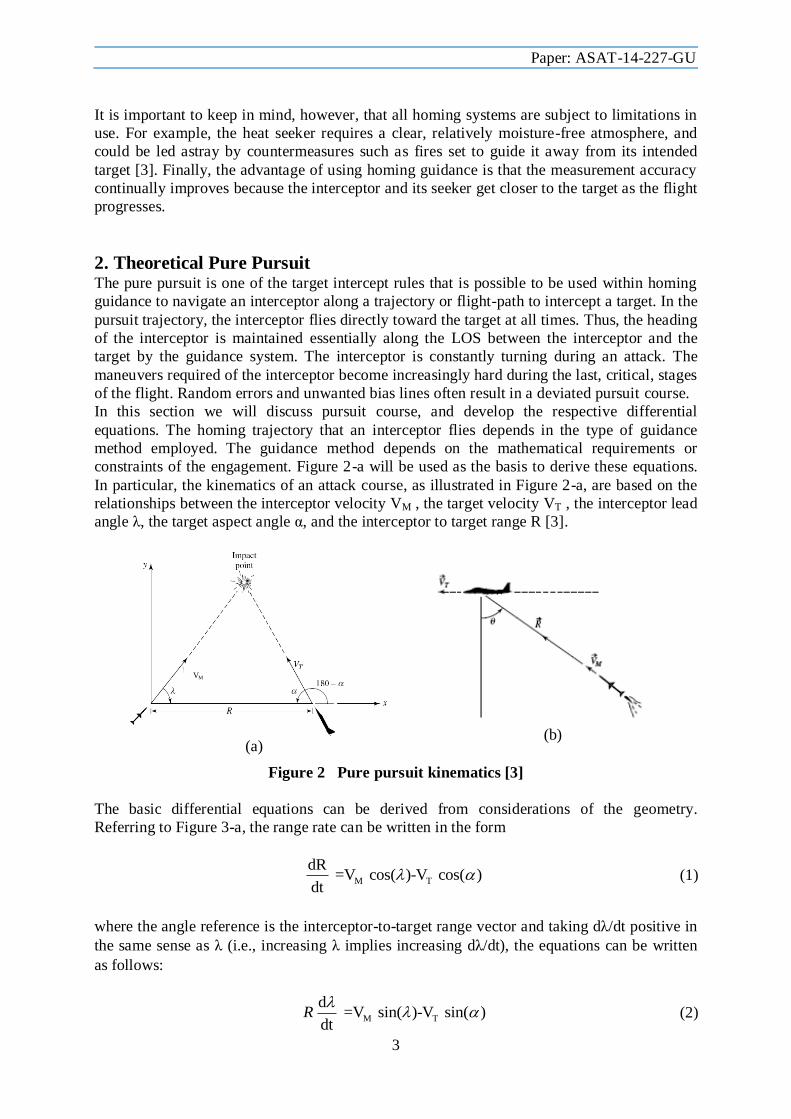
constraints of the engagement. Figure 2-a will be used as the basis to derive these equations.

In particular, the kinematics of an attack course, as illustrated in Figure 2-a, are based on the

relationships between the interceptor velocity VM , the target velocity VT , the interceptor lead

angle λ, the target aspect angle α, and the interceptor to target range R [3].

(a)

(b)

Figure 2 Pure pursuit kinematics [3]

The basic differential equations can be derived from considerations of the geometry.

Referring to Figure 3-a, the range rate can be written in the form

M T

dR =V cos( )-V cos( )

dt (1)

where the angle reference is the interceptor-to-target range vector and taking dλ/dt positive in

the same sense as λ (i.e., increasing λ implies increasing dλ/dt), the equations can be written

as follows:

M T

d =V sin( )-V sin( )

dtR

(2)

VM

Paper: ASAT-14-227-GU

4

The conditions for the various types of trajectories are resulted from holding constant one of

the parameters in the equations. In case of pure pursuit consider Figure 2-b. The

decomposition of the velocity vector components along and perpendicular to R yields the

following equations:

M T

dR =V -V sin( )

dt (3)

T

d = -V cos( )

dtR

(4)

For the planar case and non-maneuvering target, the kinematics of trajectories produced when

interceptor pursues target following the pure pursuit geometry rule. Let our plane be the z=0

plane of a Cartesian frame of coordinates. Assume that the target move along the line xT(t) =

D, where D is a constant, yT(t) = vT * t. Suppose the interceptor start pursuing the target from

the origin, i.e., xM(t) = 0, yM(t) =0, and that the velocity ratio k= vM / vT is constant. Bouger

[5] has shown that the interceptor trajectory yM(xM) is given by the following equation

k 1 k 1

k kM M M

2

y x xk 1 0.5 (k-1) 1- - (k 1) 1-

D (k -1) D D

(5)

Trajectories obtained by eqn 5 are shown in the following figure for four values of k.

Figure 3 Pure pursuit interceptor path

3. Simulation of sound tracking pure pursuit In this section there is a simulation to show how an interceptor carry an array of sensors can

intercept a moving target by its sound. The interceptor will follow pure pursuit as a guidance

rule. Actually the interceptor will follow deviated pure pursuit. There are two reasons for this.

The first one is the dynamic response of the interceptor. The second reason is the virtual target

position which comes as a result of the delay that occurs between the emitting of the target

sound signal and receiving this signal by the interceptor (figure 4).

0 0.1 0.2 0.3 0.4 0.5 0.6 0.7 0.8 0.9 10

0.2

0.4

0.6

0.8

1

1.2

1.4

1.6

1.8

2

x/c

y/c

k=2

k=1.5

k=1.2

k=1

Target path

x/D

y/D

Paper: ASAT-14-227-GU

5

Figure 4 Virtual target position

There are several steps to perform this simulation. First select some simulation parameters

(Target velocity vT, Ratio of the interceptor velocity to the target velocity vM/vT, The initial

positions of the target (xT(1), yT(1)) and the interceptor (xM(1), yM(1)), The initial orientation of

the target and interceptor w. r. t. the fixed frame of axis θT(1) and θM(1), And so the rate of

change of the target angle dθT/dt which determine the degree of the target maneuverability).

The simulation of the interceptor starts after the target simulation with the time required to the

wave travelling from the initial position of the target to the initial position of the interceptor

tdelay.

2 2

(1) (1) (1) (1)delay T M T Mt x x y y c (6)

c is the speed of sound. The simulation iteration is done each dt (sampling time of the racking

loop). Each iteration of the simulation contains calculation procedure to get the position and

orientation of the target and interceptor for the next iteration. The procedure of the calculation

of the iteration number n starts with searching the target path to get the target position that the

interceptor can sense, and this is by calculate the distance d for each target position.

2 2

(1... ) (1... ) ( ) (1... ) ( ) ( ...1)T M T Md n x n x n y n y n n dt c (7)

The target position that achieve the minimum distance d is the virtual target position that is

sensed by the interceptor at the iteration number n, suppose this is the target position at

iteration number ndmin < n. The target angle (source angle) θ(n) is calculated using ndmin.

1

min min( ) ( ) tan ( ) ( ) ( ) ( )M T d M T d Mn n y n y n x n x n (8)

The sound pressure signals that should be measured by the sensor of the array and come from

sound source located on angle θ(n) w. r. t. the array are built, and some noise is added in this

signal. These signals are used in the array of sensors calculation to get the output angle. This

angle is filtered to get the filtered angle θfiltered(n) by using Kalman filter. The position and

orientation of the target and interceptor for the next iteration are calculated as follow.

Paper: ASAT-14-227-GU

6

( 1) ( ) ( )M M dyn filteredn n K n (9)

( 1) ( ) TT T

dn n dt

dt

(10)

( 1) ( ) cos ( 1)T T T Tx n x n v dt n (11)

( 1) ( ) sin ( 1)T T T Ty n y n v dt n (12)

( 1) ( ) cos ( 1)M M M Mx n x n v dt n (13)

( 1) ( ) sin ( 1)M M M My n y n v dt n (14)

Kdyn represents the deviation part in the pure pursuit that come from the interceptor

dynamics. The simulation stops when the distance between the target and interceptor becomes

less than a certain accepted value or when the number of iterations exceeds the specified limit.

Several simulations were done with different parameters. All the simulations were done in air

with sound speed 340m/sec. Figure 5-a shows the simulation using target velocity vT =

100m/sec, ratio of the interceptor velocity to the target velocity vM/vT =2, the initial positions

of the target (xT(1), yT(1)) =(1000, 0) and the interceptor (xM(1), yM(1)) = (0, 0), the initial

orientation of the target and interceptor with respect to the fixed frame of axis θT(1) = 90o and

θM(1) =0o, and the rate of the target angle dθT/dt = 0.

The comparison between the simulated interceptor path and the theoretical interceptor path

shows the simulated path is larger than the theoretical path in distance and interception time.

The reasons of the delay in the simulated are as follow. The interceptor does not sense

immediately the target position but senses the virtual target position. The second reason is the

presence of noise. The last one is the interceptor dynamics which cause some delay until the

interceptor reaches the required position. Figure 5-b shows the variation of the target angle θ

with time during the simulation. The maximum target angle occurs at the end of the path

which is matched with the theory.

Another set of simulations were done with the same parameters that were used in the previous

simulation but with different value for dθT/dt to simulate a maneuvering target. Figures 6-a

and 6-b show the simulation results for maneuvering target that outgoing from the interceptor

with dθT/dt = -5 deg/sec. Figures 7-a and 7-b show the simulation results for maneuvering

target that incoming to the interceptor with dθT/dt = 5 deg/sec.

In case of maneuvering target that outgoing from the interceptor, the maximum target angle

that occurs at the end of the path is less than the maximum target angle that occurs in case of

the non-maneuvering target. In case of maneuvering target that incoming to the interceptor,

the maximum target angle that occurs at the end of the path is greater than the maximum

target angle that occurs in case of the non-maneuvering target. It could be concluded that as

the target approach in its maneuver as the interceptor difficultly intercept it.

Paper: ASAT-14-227-GU

7

(a) (b)

Figure 5 Pure pursuit using microphone array for non-maneuvering target

(a)

(b)

Figure 6 Pure pursuit using microphone array for maneuvering target

with dθT/dt = -5 deg/s

(a)

(b)

Figure 7 Pure pursuit using microphone array for maneuvering target with dθT/dt = 5

deg/sec

-200 0 200 400 600 800 1000 1200

0

200

400

600

800

1000

X (m)

Y

(m)

Target path v T =100m/sec

Interceptor path v m =200m/sec

Target final position Interceptor final position Theoretical interceptor path

2 3 4 5 6 7 8 9 10 11 12-15

-10

-5

0

5

10

15

20

25

30

time (sec)

angle

(deg)

unfiltered angle

correct angle

filtered angle

0 200 400 600 800 1000 1200 1400 1600

0

200

400

600

800

1000

X (m)

Y (

m)

Target path vT=100m/sec

interceptor path vm

=200m/sec

Target final position

interceptor final position

2 4 6 8 10 12 14-15

-10

-5

0

5

10

15

20

time (sec)

angle

(deg)

unfiltered angle

correct angle

filtered angle

0 100 200 300 400 500 600 700 800 900 10000

100

200

300

400

500

600

700

800

X (m)

Y (

m)

Target path vT=100m/sec

interceptor path vm

=200m/sec

Target final position

interceptor final position

2 3 4 5 6 7 8 9 10 11-20

0

20

40

60

80

100

time (sec)

angle

(deg)

unfiltered angle

correct angle

filtered angle

Paper: ASAT-14-227-GU

8

Another simulation was done with the same parameters but for supersonic target and

interceptor speeds vT = 500m/sec. the case of maneuvering target that approach to the

interceptor with dθT/dt =5 deg/sec was studied, figure 8.

Figure 8 Pure pursuit using microphone array for maneuvering target with dθT/dt = 5

deg/sec

There is a problem occurred in the supersonic simulation. The interceptor turned backward,

because it received a sound signal from the back. This is possible when the speeds of the

target and interceptor are greater than the speed of sound so the interceptor can receive sound

signal and then turn out this signal and receive this again in another position, figure 9. This

problem may be solved by isolating the sound signals that come from the backward direction

of the interceptor by any mean of sound isolation. The results of this are shown in figure 10.

Figure 9 Supersonic sound tracking

0 100 200 300 400 500 600 700 800 900 1000-500

0

500

1000

1500

2000

2500

3000

3500

X (m)

Y (

m)

Target path v

T=500m/sec

interceptor path vm

=1000m/sec

Target final position

interceptor final position

Paper: ASAT-14-227-GU

9

Figure 10 Supersonic sound tracking with backward signal isolation

An important note may be found by performing the simulation of non maneuvering target

with various ratios of the target velocity vT to the speed of sound c and constant vm/vT ratio.

The note is that as the speed ratios of target and interceptor relative to the speed of sound are

larger, then the simulated path is larger than the theoretical path in distance and intercepting

time. Figure 11 also shows that as the speed ratios of the target and the interceptor relative to

the speed of sound are smaller, then the simulated interceptor path approach the theoretical

interceptor path.

Figure 11 The effect of the speed ratios of target and interceptor relative to the speed of

sound on the interceptor path

-1500 -1000 -500 0 500 1000 1500 2000 25000

500

1000

1500

2000

2500

3000

X (m)

Y (

m)

Target path vT=500m/sec

interceptor path vm

=1000m/sec

Target final position

interceptor final position

-0.2 0 0.2 0.4 0.6 0.8 10

0.5

1

1.5

2

2.5

3

3.5

x/xt(0)

y/x

t(0)

Target path

interceptor path vm

= 1.5 vT , v

T =10c

interceptor path vm

= 1.5 vT , v

T =5c

interceptor path vm

= 1.5 vT , v

T =c

interceptor path vm

= 1.5 vT , v

T =0.1c

theoretical interceptor path vm

=1.5 vT

Paper: ASAT-14-227-GU

10

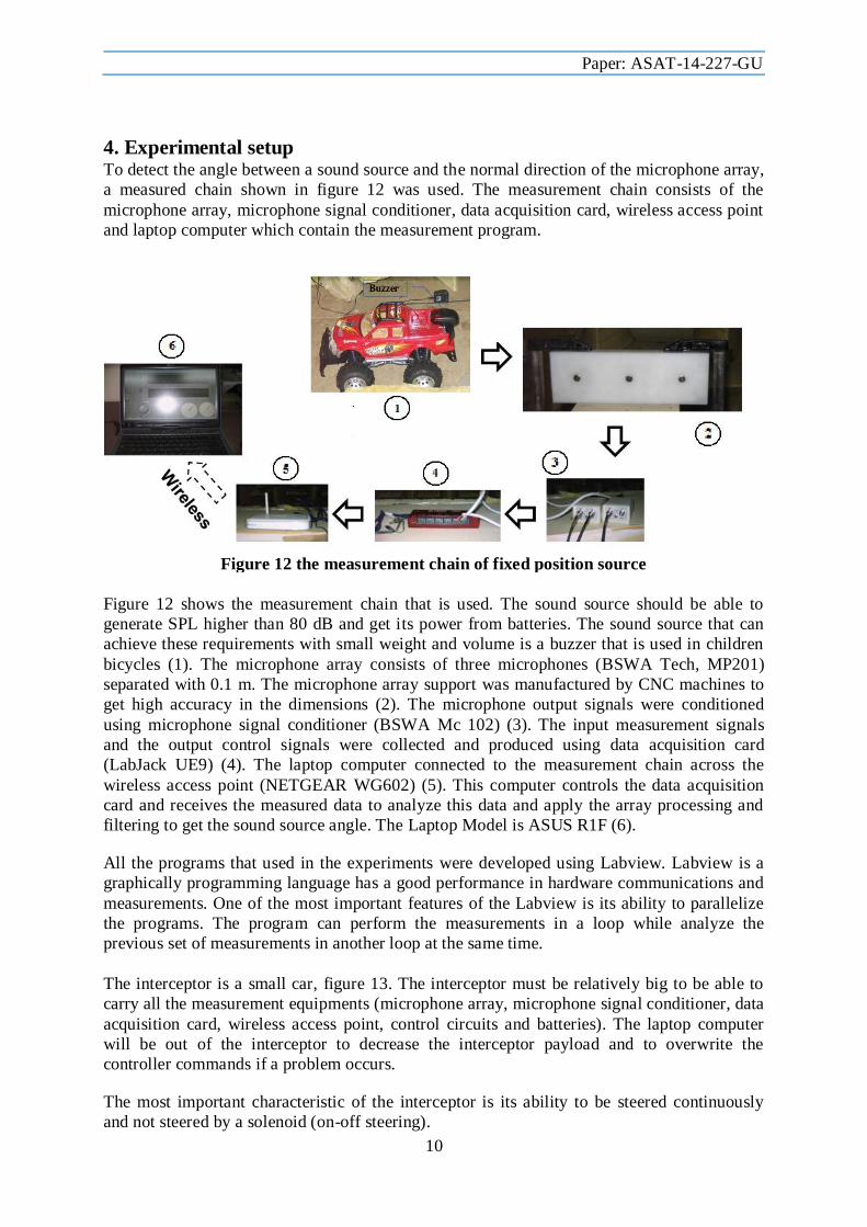
4. Experimental setup To detect the angle between a sound source and the normal direction of the microphone array,

a measured chain shown in figure 12 was used. The measurement chain consists of the

microphone array, microphone signal conditioner, data acquisition card, wireless access point

and laptop computer which contain the measurement program.

Figure 12 the measurement chain of fixed position source

Figure 12 shows the measurement chain that is used. The sound source should be able to

generate SPL higher than 80 dB and get its power from batteries. The sound source that can

achieve these requirements with small weight and volume is a buzzer that is used in children

bicycles (1). The microphone array consists of three microphones (BSWA Tech, MP201)

separated with 0.1 m. The microphone array support was manufactured by CNC machines to

get high accuracy in the dimensions (2). The microphone output signals were conditioned

using microphone signal conditioner (BSWA Mc 102) (3). The input measurement signals

and the output control signals were collected and produced using data acquisition card

(LabJack UE9) (4). The laptop computer connected to the measurement chain across the

wireless access point (NETGEAR WG602) (5). This computer controls the data acquisition

card and receives the measured data to analyze this data and apply the array processing and

filtering to get the sound source angle. The Laptop Model is ASUS R1F (6).

All the programs that used in the experiments were developed using Labview. Labview is a

graphically programming language has a good performance in hardware communications and

measurements. One of the most important features of the Labview is its ability to parallelize

the programs. The program can perform the measurements in a loop while analyze the

previous set of measurements in another loop at the same time.

The interceptor is a small car, figure 13. The interceptor must be relatively big to be able to

carry all the measurement equipments (microphone array, microphone signal conditioner, data

acquisition card, wireless access point, control circuits and batteries). The laptop computer

will be out of the interceptor to decrease the interceptor payload and to overwrite the

controller commands if a problem occurs.

The most important characteristic of the interceptor is its ability to be steered continuously

and not steered by a solenoid (on-off steering).

Paper: ASAT-14-227-GU

11

Figure 13 interceptor car

5. The guidance loop The guidance loop starts with the angle measurement system. The array of sensor is fixed on

the interceptor where the normal direction of the array matches the roll axis of the interceptor.

The measured angle θ represents the error angle between the line of sight LOS and the

interceptor roll axis. The error angle θ passes through the filter. The filter output is used to get

the controller action. The data acquisition card outs the value of the controller action to the

pulse width modulation circuit which controls the speed of the steering motor.

Figure 14 guidance loop

Figure 14 shows the guidance loop. The guidance loop consists of six elements starting with

filtering. The filtering process is a Kalman filter. The output of the filtering process passes

through the controller. The controller that used is a gain scheduling PD controller with two

regions. The control action goes to the pulse width modulation circuit (PWM), this control

circuit is ideal for accurate control of DC motors. The circuit converts a DC voltage into a

series of pulses, such that the pulse duration is directly proportional to the value of the DC

voltage. The PWM circuit that used is VELLEMAN K8004. The output of the PWM goes to

the switching circuit to control the steering direction. The switching circuit consists of relays

and optocouplers. The optocouplers take digital commands from some digital outputs of the

data acquisition card and path it to the relays coils. The relays change the polarity of the

Paper: ASAT-14-227-GU

12

steering motor so it can determine the steering direction (left or right), where the PWM only

control the analog value without direction. The second function of the switching circuit is to

turn on the motor of the forward motion of the interceptor at the start of the experiment and

turn it off at the end of the experiment. The steering motor produces steering angular velocity.

The output of the steering system is the steering angle. The car dynamics produces yawing

angular velocity. The output of the guidance loop is the interceptor yaw angle θM.

6. Experimental results In this experiment the target moved in random motion with average speed 0.8 m/sec which is

less than the interceptor speed 1.2 m/sec. The results of this are shown in a video and the

equipments required to compute the path of the interceptor and target were not available. For

this reason a simpler experiment was performed in which the target moved along a uniform

path in a straight line, and the interceptor was released three times from the origin to ensure

repeatability of the experiment. The path of the interceptor was traced using chalk, because

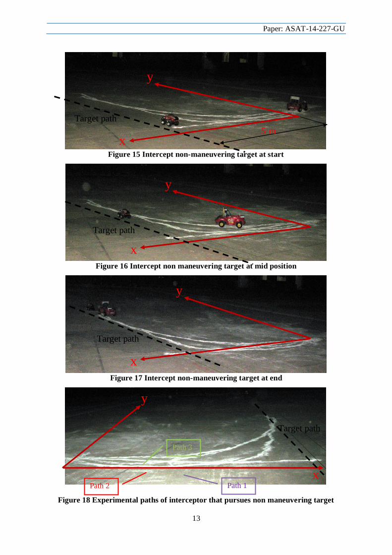
there were unavailable sensors to measure the exact location. Figures 15, 16 and 17 show the

path of the interceptor as it pursues the non maneuvering target along the straight line.

Some points were measured for each path to compare it with the theoretical path and

simulated path. Figure 19 shows the measured, theoretical and simulated paths. Because of

the low speeds of the target and interceptor relative to the speed of sound, all of the paths

reach the target path almost at the same position. Some delay in the experimental paths

because of the dynamic response of the interceptor. At start of the experiment the paths of the

experiments were different as results of sound reflections, background noise and the initial

steering angle of the interceptor which is different for each trial with small error.

7. Conclusions The strongest and most important statement that can be made from the results observations is

sound tracking is promising. Also the most important observations can be concluded in the

following. The effect of the virtual target position makes the path of pure pursuit with sound

tracking larger than the theoretical pure pursuit path in distance and interception time. The

required interceptor maneuvers are rapidly increased as the target maneuvers approach the

interceptor. The path (distance and intercepting time) of the sound tracking pure pursuit is

increased as the speed ratios of the target and the interceptor relative to the speed of sound are

increased, and the path approaches the theoretical path as the speed ratios are decreased. It is

important to isolate the sound signals that come from the backward direction of the

interceptor if the speeds of the target and interceptor are greater than the speed of sound. The

dynamic response of the interceptor makes some delay in the experimental paths. The

measurement noise and initial steering error make some differences at the starting of the

experimental paths.

8. Acknowledgement Many thanks go out to all the staff of the Group for Advanced Research in Dynamic Systems

Ain-Shams University “ASU GARDS” where all the experimental work were done and

supporting with hardware and facilities that were needed.

Paper: ASAT-14-227-GU

13

Figure 15 Intercept non-maneuvering target at start

Figure 16 Intercept non maneuvering target at mid position

Figure 17 Intercept non-maneuvering target at end

Figure 18 Experimental paths of interceptor that pursues non maneuvering target

x

y

5 m

m

Target path

x

y

Target path

x

y

Target path

x

y

Target path

Path 1 Path 2

Path 3

Paper: ASAT-14-227-GU

14

Figure 19 Pure pursuit paths

9. References [1] John H. Blakelock, “Guided Automatic Control of Aircraft and Missiles,”, Second

Edition, Wiley, New York, 1965.

[2] D. W. LADD and E. W. WOLF, “A Non-Real-Time Simulation of SAGE Tracking and

BOMARC Guidance,” ”, Electronic Computers, IRE Transactions on,” March 1959,

Volume EC-8, Issue 1, pp. 36-41.

[3] George M. Siouris, Missile Guidance and Control Systems, 2004.

[4] Jung-Min Pak, Dong-Gi Woo, Bonhwa Ku, Wooyoung Hong, Hanseok Ko and Myo-

Taeg Lim, “Target Search Method for a Torpedo to the Evading Ship Using Fuzzy

Inference,” ”, ICCAS-SICE, 2009,” 18-21 Aug, pp. 5279 - 5284.

[5] N. A. Shneydor, Missile Guidance and Pursuit Kinematics, Dynamics and control,

1998.

[6] P. Garnell, Guided Weapon Control System, Second Edition, 1980.

[7] Alan V. Oppenheim, Alan S. Willsky, and S. Hamid Nawab, Signals and Systems,

Second Edition, 1997.

[8] David M. Auslander, John R. Ridgely, and Jason C. Jones, Real Time Software for

Implementation of Feedback Control.

[9] Klaas B. Klaassen, Electronic Measurement and Instrumentation, 1996.

[10] Philip Denbigh, System Analysis and Signal Processing, 1998.

0 1 2 3 4 5 6-1

0

1

2

3

4

5

6

7

x

y

Measured interceptor path 1

Measured interceptor path 2

Measured interceptor path 3

Theoretical interceptor path

Simulated interceptor path

Target path