HAL Id: hal-00521190https://hal.archives-ouvertes.fr/hal-00521190

Submitted on 26 Sep 2010

HAL is a multi-disciplinary open accessarchive for the deposit and dissemination of sci-entific research documents, whether they are pub-lished or not. The documents may come fromteaching and research institutions in France orabroad, or from public or private research centers.

L’archive ouverte pluridisciplinaire HAL, estdestinée au dépôt et à la diffusion de documentsscientifiques de niveau recherche, publiés ou non,émanant des établissements d’enseignement et derecherche français ou étrangers, des laboratoirespublics ou privés.

Analysis and artifact correction for volume correlationmeasurements using tomographic images from a

laboratory X-ray sourceNathalie Limodin, Julien Réthoré, Jérôme Adrien, Jean-Yves Buffière,

François Hild, Stéphane Roux

To cite this version:Nathalie Limodin, Julien Réthoré, Jérôme Adrien, Jean-Yves Buffière, François Hild, et al.. Analysisand artifact correction for volume correlation measurements using tomographic images from a lab-oratory X-ray source. Experimental Mechanics, Society for Experimental Mechanics, 2011, 51 (6),pp.959-970. <10.1007/s11340-010-9397-4>. <hal-00521190>

Experimental Mechanics manuscript No.(will be inserted by the editor)

Analysis and artifact correction for volume correlation

measurements using tomographic images from a laboratory

X-ray source

Nathalie Limodin Julien Rethore Jerome

Adrien Jean-Yves Buffiere Francois Hild

S. Roux

Received: date / Accepted: date

Abstract The effects of three artifacts (reconstruction, beam hardening and temper-

ature of the X-ray tube) associated with the use of a lab tomograph are analyzed in

terms of their induced biases for Digital Volume Correlation (DVC) from a series of

reconstructed volumes acquired successively. The most detrimental effect is due to spu-

rious dilatational strains induced by temperature variations in the tomograph. If they

N. Limodin, J. Adrien, J.-Y. Buffiere

Laboratoire Materiaux, Ingenierie et Sciences (MATEIS)

INSA-Lyon / UMR CNRS 5510

7, avenue Jean Capelle, F-69621 Villeurbanne, France

E-mail: nathalie.limodin,jerome.adrien,jen-yves.buffiere@insa-lyon.fr

J. Rethore

Laboratoire de Mecanique des Contacts et des Structures (LaMCoS)

INSA-Lyon / UMR CNRS 5259

20 avenue Albert Einstein, F-69621 Villeurbanne, France

E-mail: julien.rethore@insa-lyon.fr

F. Hild?, S. Roux

Laboratoire de Mecanique et Technologie (LMT-Cachan)

ENS Cachan / CNRS / UPMC / PRES UniverSud Paris

61 Avenue du President Wilson, F-94235 Cachan Cedex, France

?corresponding author

E-mail: francois.hild,stephane.roux@lmt.ens-cachan.fr

2

are not accounted for, any quantitative kinematic measurement is impossible for strain

levels below 0.5 %.

Keywords Quantitative kinematic measurements · Reconstruction artifacts ·Thermal expansion · X-ray computed microtomography

1 Introduction

To visualize inside opaque materials, X-ray computed microtomography (XCMT) has

become more and more popular since its invention more than thirty years ago [1,2]. 3D

views of various materials [3,4] are obtained in a non-destructive way. Reconstructed

volumes give invaluable indications on the structure of metallic [5], ceramic [6,7], ce-

mentitious [8], cellular [9] materials. Damage mechanisms [10,11] and cracks [12,13]

are also analyzed through direct visualization.

It is also possible to load samples in situ [14]. An additional analysis consists in

using the reconstructed volumes themselves to evaluate displacements. The latter are

for instance measured by resorting to marker tracking [15]. Another technique consists

in local correlations [16,17], in which small interrogation volumes in two scans are

registered [18]. An alternative route to local approaches is provided by global correlation

techniques [19,20,21,22]. The latter will be used herein. In all these cases, the kinematic

analysis relies on scans taken at different times. Consequently, they may be corrupted

by various phenomena such as reconstruction artifacts, beam hardening, and (for a

cone-beam geometry) uncontrolled motion of the source with respect to the sample due

to thermal expansion of the set-up during operation. This is the case of lab tomographs.

In Section 2, the main causes of artifacts related to tomography are discussed.

Section 3 introduces the basic principles of volume correlation. The way the measured

displacements are post-processed to evaluate the effect of different artifacts is dis-

cussed. Section 4 is devoted to the effect of temperature variations of the X-ray tube

on measured displacements. In Section 5, the effect of reconstruction (so-called ring)

artifacts on the performance in terms of standard displacement uncertainty is assessed.

3

The influence of beam hardening corrections are studied in Section 6. Last, all these

effects are finally considered in Section 7 when a tensile test on nodular graphite cast

iron is performed. In particular, the extraction of elastic parameters is discussed and

correction procedures are validated.

2 Tomography

In the present section, the basic principles of X-ray tomographic imaging are briefly

summarized (see for example [23,24] for an exhaustive presentation of the technique)

and the specificities of a tomography set-up that uses a laboratory micro-focus X-ray

source (lab-CT) are analyzed with an emphasis on artifacts arising from this kind of

device.

Because tomography is a non destructive technique, the changes in a sample sub-

mitted to various experimental environments can be studied in situ with a volume

large enough to yield statistically relevant information. Therefore, in the last 15 years,

X-ray CT, originally developed for studies in the medical field, has found more and

more applications in materials science (see for example [25] for a recent review of var-

ious applications). This increasing interest in tomography and the difficulty to have

access to synchrotron facilities have prompted for lab-CT development. This tool has

now become widespread for materials characterization, and a precise knowledge of its

possibilities and limitations is mandatory whenever accurate and quantitative results

are sought.

Although various experimental set-ups are used to perform X-ray tomography, the

basic principles of the technique remain the same, namely, an X-ray beam is sent

onto a sample mounted on a rotator, a series of N radiographs (herein called a scan)

corresponding to N angular positions of the sample (360 rotation in the case of lab-

CT) in the beam is recorded on a detector that is generally a CCD camera in modern

tomographs. Those radiographs are used by a reconstruction software to obtain the

3D distribution of the linear X-ray attenuation coefficient µ within the sample. This

distribution forms the 3D reconstructed volume. The value of µ depends on the X-

4

ray photon energy as well as on the material density and atomic number so that the

contrast in CT images is usually given by differences in absorption between phases or

constituents with different compositions or densities.

A lab-scale tomograph is composed of a source, i.e., an X-ray tube (micro- or

nanofocus), a sample manipulation system that allows for accurate positioning and

motion of the sample (3 translations + 1 rotation). A 2D flat panel detector con-

verts X-rays into digital radiographs stored in a computer. The X-ray tube produces a

polychromatic and conical beam whose divergence is used to monitor the image magni-

fication by moving the object relative to the source (the magnification equals the source

to detector distance divided by the source to sample distance). The spatial resolution

is however limited by the size of the focal spot due to a penumbral blurring effect. A

smaller spot size is required for high resolution images, at the expense of the delivered

flux (inducing longer scan times).

One of the most basic artifact that are found in tomographic images is caused by

the reconstruction software using a wrong reconstruction axis. Hence, prior to recon-

struction, the position of the projection on the CCD detector of the sample rotation

axis has to be determined accurately. The determination of the “actual” position of the

rotation axis is usually left to the user who eventually validates visually the software

alignment procedure by looking at reconstructed slices.

Another so-called “ring-artifact” is also frequently observed in tomographic images.

Among other causes, it may be due to defective elements of the detector (e.g., elements

delivering a non-linear signal) or inhomogeneities in the X-ray beam. Such defects

appear on each recorded projection of the sample and produce a ring-shaped contrast

centered on the rotation axis in the reconstructed image. Because of the higher angular

sampling of the sample close to the rotation axis, ring artifacts are more pronounced

towards the rotation axis. A flat-field correction routinely applied on the projections

using the “offset” and “gain” images recorded at the beginning of the scan is generally

not sufficient to erase these artifacts. These rings may be detrimental to subsequent

processing, e.g., segmentation, and thus to quantitative image analyses. The techniques

5

used to remove or minimize these rings are divided into two categories, namely, i) post-

processing of the reconstructed data, i.e., filtering, but then part of the contrast due

to high frequency features can be lost [27], and ii) pre-processing of the data prior to

reconstruction, i.e., sinogram processing [28,29].

The polychromatic X-ray beam used by lab-CT equipments is the source of another

type of artifact called beam hardening. The polychromatic beam, when traversing a

sample, loses the less energetic of its photons that are absorbed, and therefore the

mean energy of the transmitted X-ray beam is higher than that of the incident beam.

In practice, long ray paths being more attenuating than short ones, an artificial dark-

ening (resp. brightening) at the centre (resp. edges) of the sample is observed on the

reconstructed images impeding, for example, a direct conversion of the gray levels in

values of the attenuation coefficient µ. Several solutions have been proposed to reduce

beam hardening artifacts, the most classical of which consists in using a thin metallic

foil (typically 1 mm-thick or less of copper or aluminium sheets) to filter or “pre-

harden” the beam. The price to pay for this filtering is a decrease in X-ray flux that

might result in a lower signal to noise ratio.

Imperfect motions of the rotation stage, motions of the specimen (e.g., insufficiently

clamped specimens or living specimens) and motions of the X-ray emission spot are

also sources of artifacts on reconstructed images. The sample translations that occur

during a scan due to mechanical instabilities or inaccuracies of the sample translations

are compensated for by processing the projections. For example, in the reconstruction

software used in this work, an image compensation routine allows for “manual” correc-

tions to be applied, namely, shifting and scaling of the last projection (360) is applied

by the user until a good match (assessed by eye) is obtained with the first projection

(0). However, no correction is possible for a tilt that would arise from wobble or ec-

centricity of the rotator or sample mount. Such artifacts are all the more important

when the magnification is high. For nanofocus tubes that enable for magnifications up

to 1000, air bearings and piezo elements are preferred for accurate sample rotation and

manipulation.

6

In lab-CT, only a small fraction of the energy of the electron beam impinging on

the W target is converted into X-rays, the remainder is dissipated into heat. During

a scan acquisition, X-rays are continuously emitted for several tens of minutes and

the temperature of the X-ray tube may increase by about 10 C. If several scans are

performed in a row, as usually occurring during in situ studies, the X-ray tube has

no time to cool down after one scan, and its temperature increases with the number

of scans, i.e., with time. The situation is exactly similar in the case of a single long

scan, which is often necessary when high resolution (voxel size < 1µm) is sought.

This increase in temperature induces thermal expansion of the X-ray tube assembly.

In turn, thermal dilation causes small geometric motions of the X-ray emission point.

These motions can occur in the plane perpendicular to the beam or parallel to it. In

the latter case, the source to sample distance steadily decreases during the scan and

alters the magnification of the recorded radiographs. Although the displacement of the

X-ray tube with respect to the sample is very small, its effect on the radiographs is

amplified by geometrical magnification.

In practice, therefore, images with resolutions in the micrometer or sub-micrometer

range require that the temperature variation and subsequent expansion of the tube are

either controlled or corrected prior to reconstruction. Salmon et al. [30] have proposed

to correct shifts in the plane perpendicular to the X ray beam on individual radio-

graphs. The shifts are determined by registering the nth radiograph of the scan with

the corresponding one (same angular position) of a fast scan (a few angular positions)

recorded at the end of the experiment. This correction procedure increases the qual-

ity of images and has also an effect on the recorded gray level histograms of various

samples / materials. The motions of the source along the beam direction are however

not considered by the authors. It will be shown in Section 4 that such motions are also

to be taken into account when successive reconstructions or scans are to be compared

quantitatively.

The experiments reported in this study are performed using a CT system V-Tomex

(Phoenix X-ray) fitted with a nanofocus tube (W target) whose acceleration voltage is

7

adjusted from 40 to 160 kV, and whose focal spot size is tuneable from 6 µm to 1 µm.

The material of the present study, i.e., cast iron (see reference [21] for a description

of the material), being strongly attenuating, the tomography experiments are carried

out with a rather large spot size, i.e., 3.5 µm, and a 95 kV acceleration voltage to

ensure a 10 % transmission of the X-ray beam through the 1.5 × 1.5 mm2 cross-

section of the sample. The specimen is put on the rotating stage (wobble: ±7 µrad,

eccentricity: ±0.4 µm, uncertainty of angular positioning: 130 µrad) in the tomograph

chamber between the X-ray source and an amorphous Si diode array detector of di-

mensions 1920 × 1536 pixels. A set of 900 radiographs is recorded while the sample

is rotating, step by step, over 360 along its vertical axis. When the radiograph is

shot, the rotating stage does not move. With an acquisition time per image of 500 ms,

one scan lasted about 45 min. A small tensile testing device was used to load the

specimen for in situ test [21]. This device uses a glass cylinder to transmit the load

between the top and bottom parts of the machine, and therefore imposes a minimum

source to specimen distance of 15.9 mm. This condition results in an image voxel size

of 3.5 µm. Reconstruction of the tomographic data is performed with a filtered back-

projection algorithm (i.e., an optimized Feldkamp cone-beam algorithm [31]) using

datos x-acquisition and reconstruction software developed by Phoenix. It provides a

3D image with a 16-bit deep gray scale (Figure 1).

Although artifacts possibly affecting image reconstructions have been listed above,

reconstructed images will be trusted in the sequel (without specific pre-corrections) but

compared to each other to evaluate displacements by resorting to volume correlation.

Consequences in terms of sinogram pre-corrections, albeit certainly desirable, will not

be investigated herein.

3 Volume Correlation

A reconstructed volume is represented as a discrete function f(x) giving the gray level

at each voxel position x. For the ease of presentation, such functions will be consid-

ered as the discrete sampling of a continuous (interpolated) function. Digital volume

8

correlation (DVC) consists in registering two volumes with the help of a displacement

field to be measured. The conservation of the local texture between the reference f and

deformed g volumes is given by

g(x + u(x)) = f(x) (1)

where x is the position vector, and u the sought displacement vector. The texture

conservation hypothesis is not strictly satisfied. In particular, 3D volumes obtained by

XCMT are the results of a numerical reconstruction procedure that induces artifacts

listed in Section 2. The difference, g(x+u(x))−f(x), or correlation residuals, quantifies

the quality of volume registration.

When two volumes f and g are considered, the measurement problem consists in

evaluating u as accurately as possible. To measure u, the quadratic difference ϕ2 =

[g(x + u(x))− f(x)]2 is integrated over the studied domain Ω

Φ2 =

Z

Ωϕ2dx (2)

and minimized with respect to the unknown degrees of freedom of the measured dis-

placement field. In the following, a 3D finite element kinematics is selected for the

sought displacement field u. The simplest shape functions are used, namely, trilinear

polynomials associated with 8-node cube elements (or C8-DVC). More details on the

correlation procedure can be found in Ref. [19]. The size of each element is denoted by

` so that the total number of voxels per element is `3.

DVC is used in order to extract significant mechanical quantities from experi-

ments [32,21,22]. In the present study this tool is utilized to analyze and possibly

correct for artifacts due to reconstruction and/or temperature variations of the X-ray

tube. In the following sections two types of analyses are used:

– when a rigid body motion is applied to the sample, the mean and root mean square

(RMS) of the displacement field are assessed. The standard displacement uncer-

tainty is then interpreted as a global evaluation of the measurement uncertainty

and some additional effects that call for corrections, whenever possible,

9

– once the effect of an artifact has been included, or when the actual displacement

is not simply a rigid body translation, corrections are proposed to reduce mea-

surement “errors.” The measured displacement is then projected onto a basis that

contains the rigid body motion and the suspected field associated with an artifact

ui(x) = u0 + x× ! + ε x (3)

where ui is the interpolating displacement field, u0 the mean translation, ! the cor-

responding rotation vector, and ε the dilatational strain component. After the con-

tribution of each of these elementary displacements has been calculated by means

of a least squares minimization, the RMS of the difference between measured and

interpolating displacement fields quantifies the effect of the proposed correction.

This strategy is successively applied to quantify and further correct the effect of

temperature variations of the X-ray tube, ring artifacts, and beam hardening.

4 Temperature variations of the X-ray tube

In the present operating conditions, acquiring a complete scan of a sample lasts typ-

ically 45 minutes. If several scans are acquired successively, X-rays are emitted for

about an entire day so that the temperature of the tube may vary by several tens

of Celsius degrees from the first to the last scan. Variations of magnification between

each radiograph, and more importantly between two scans are therefore expected. This

may impact quantitatively the procedures of tomographic image acquisition with a lab

tomograph that is not running 24 h / day.

The following analysis is proposed to quantify this effect. A series of scans of the

same unloaded sample are acquired successively. The sample was not moved. The dis-

placement fields with respect to the very first scan are measured by using DVC and

further processed. Due to the variation of the magnification induced by the temper-

ature variation of the X-ray tube, an homothetic transformation is looked for. The

measured displacement field is thus projected in a least-squares sense onto a basis that

contains the rigid body motions (i.e., three translations, and three rotations) and a

10

(spurious) scalar dilatational strain ε inducing a dilatational displacement field u = εx

(see Equation (3)).

As an example, for the last scan of series #2 (Figure 3a), the following values are

obtained

ui =

266664

−3.8

10.8

−1.8

377775

| z translation

+ x× 10−5 ·

266664

24

4

−2

377775

| z rotation

+ 2.8 · 10−3 x| z dilation

(4)

with x = OM, O being the center of the region of interest, and M a current point (the

positions and displacements are expressed in voxels, where 1 voxel = 3.5 µm, and the

rotations in radian). The observed translation may be due to thermal drift of the focal

spot [30] or/and mechanical drifts of the sample and the whole mounting stage.

Figure 2 shows the norm of the displacement field when rigid body motions have

been removed, the identified spurious dilatational displacement, and the corrected dis-

placement fields. The maximum amplitude of the measured displacement is about 1.8

voxel, which is much higher than the measurement uncertainty (i.e., 0.08 voxel) of DVC

that will be assessed in Section 5. Consequently, the dilatational component cannot be

considered as a measurement uncertainty but a bias introduced by the temperature

variations of the X-ray tube. Further, after projection onto the chosen basis, the rela-

tive projection error is equal to 3.5 %, this error being defined as the ratio of the L2

norm of the difference between the initial displacement and the interpolated displace-

ment over the L2 norm of the measured displacement. This low level of the projection

error gives additional confidence in the proposed correction.

Figure 3a shows the change of the estimated dilatational strain with time for the

considered series. An exponential fit yields consistent results. The dilatational strain

depends on the thermal expansion of the X-ray tube, and the temperature of the tube

may vary exponentially with time as expected from a first order system described by

the heat equation with a loss term [33]

ε(t) = ε∞[1− exp(−t/τ)] (5)

11

where ε∞ is the steady state correction to be performed when the whole warm-up

duration is concerned. Figure 3a shows that significant levels are reached when kine-

matic measurements are sought. For instance, for an in situ tensile test the apparent

(measured) strains are expressed as

εal =

σ

E+ ε , εt

l = −νσ

E+ ε (6)

where εal is the apparent longitudinal strain, εt

l the apparent transverse strain, σ the

tensile stress, E Young’s modulus, and ν Poisson’s ratio. If cast iron is concerned as in

the present case, the longitudinal elastic strain level of a tensile test under an applied

stress of 290 MPa is of the order of 1.8 · 10−3, and the corresponding transverse strain

is equal to 5 · 10−4. These levels are less than those observed in Figure 3a. If this effect

were not corrected for, there would be no way of estimating quantitatively the elastic

properties of the considered material.

In some other cases, the reference scan is acquired at time t∆, later than the

beginning of warm-up, so that a strain increment ∆ε is to be considered

∆ε(t) = ε∞[1− exp(t∆ − t)/τ] (7)

where ε∞ has to be adjusted depending on the temperature at the time of the reference

image. In the present case no air conditioning system was used. It is assumed however

that the characteristic time τ is a constant feature of the system. The parameters ε∞

and τ are determined by considering the three previous series (Figure 3b). The values

of the steady state strain range from 3.7 ·10−3 to 4.5 ·10−3. The time t∆ is equal to 40

min for the second series, and 170 min for the third series. These values are consistent

with the time durations between the beginning of warm-up and when the acquisitions

actually started. For series #3, three scans were performed before the acquisition of the

first point of Figure 3a. The time lapse between switching on the X-ray tube and data

collection amounts to 173 min. For series #2, one scan was acquired by another user

before the experiment was started (i.e., a time lapse of 40 min). Last, the characteristic

time is equal to 130 min. This result shows that a warm-up time of about three hours is

required to avoid spurious strain levels greater than 10−3. It is confirmed by analyzing

12

the third series (Figure 3a). A warm-up time of about five hours leads to dilatational

artifacts less than 4 · 10−4 in terms of strain levels.

5 Ring artifacts

The reconstruction is an anisotropic process that distinguishes axial and radial direc-

tions (see Section 2) because of the very principle of tomography. Differences on the

uncertainty level along the rotation axis or in an orthogonal plane are expected. To

investigate this effect, a sample is translated inside the tomograph by using either the

motor-driven rotation stage or manually with the goniometer on which the sample is

mounted. Two cases are distinguished, namely, a longitudinal translation (along the

rotation axis), and a transverse translation (perpendicular to the rotation axis).

5.1 Translation along the rotation axis

The sample is translated along the rotation axis (using the motor-driven stage) by a

value of about 9 voxels. When the measured displacement field is interpolated, two or

three contributions given in Equation (3) are considered. Figure 4 shows the change of

standard displacement uncertainties prior to and after corrections as a function of the

size ` of the elements chosen for C8-DVC. For each case, the standard displacement un-

certainty is a decreasing function of the element size. When compared with the a priori

analysis for which translations are applied artificially on a ROI of 384 × 384 × 384 vox-

els (using a cubic spline interpolation of gray levels [19,22]), the uncertainty level is

significantly higher (Figure 4). Further, even though a decreasing power law is obtained

in ideal cases, a saturation of the uncertainty is observed in the experimental case.

From the raw uncertainty curve (i.e., without any rigid body and dilation correc-

tions), the correlation error is predominant for small element sizes (less than 12 voxels).

The latter arises from the fact that image correlation is an ill-posed problem, meaning

that smaller elements give less regularization and thus higher uncertainty levels are

observed [19]. For element sizes greater than 12 voxels, the influence of tomography

13

artifacts is dominant. Consequently, the standard displacement uncertainty becomes

independent of the element size.

After correcting for the dilatational strain, the saturation level of the uncertainty

is lower but still present. If the rotations are also accounted for, a further decrease of

the saturation is obtained. The rotation correction does not affect the z-component (z

being the rotation axis) but only x- and y-components. It therefore seems that ring

artifacts make the correlation algorithm detect a rotation about the rotation axis. It is

confirmed by the values of the identified rotation components when 16-voxel elements

are chosen

! = 10−5 ·

266664

−4

−2

40

377775

rad (8)

This value is significantly greater than the repositioning error (of the order 13 ·10−5 rad).

To validate this whole analysis, in particular the resolution in terms of the degrees

of freedom associated with the interpolation given in Equation (3), the displacement

uncertainty σu associated with each node of 16-voxel elements (i.e., ` = 16 voxels)

is of the order of 0.08 voxel (Figure 4). By interpolating the measured displacement

field, it is possible to evaluate an order of magnitude of the uncertainties associated

with a rotation component, say ωz , and that of ε. In the present case, the ROI is a

square containing 2n + 1 nodes (with n = 12). By neglecting the correlations between

measured degrees of freedom [34], the rotation uncertainty σω becomes

σω =σuqP

i,j,k(x2i + y2

j )(9)

and that associated with ε

σε =σuqP

i,j,k(x2i + y2

j + z2k)

(10)

When −n ≤ i, j, k ≤ n,P

i,j,k x2i =

Pi,j,k y2

j =P

i,j,k z2k = n(n + 1)(2n + 1)3`2/3.

Consequently, when σu = 0.08 voxel and n = 12, σω ≈ 4 · 10−6 rad, and σε ≈

14

3.2 · 10−6. These levels show that the values found above are significantly higher than

the resolution of the measurement technique. They are therefore deemed trustworthy.

5.2 Translation perpendicular to the rotation axis

In the same spirit as above, a translation orthogonal to the rotation axis is applied by

the operator using the manual goniometer. Figure 5 shows that without correction or

by correcting for the dilation only, the uncertainty level is higher than in the previous

case. By looking at the correlation residuals (Figure 6), two sets of rings are observed,

which means that the correlation fails at achieving a perfect match between the two

images in the regions where ring artifacts appear. This is caused by the fact that the

position of the rotation axis is different in the sample before and after its motion. It is

worth mentioning that ring artifacts are observed in the original image (Figure 1), but

they appear more clearly on the correlation residuals. After rotation correction, the

uncertainty level is similar to that observed in the previous case. This means that the

spurious rotation is even more pronounced in the case of a translation orthogonal to

the rotation axis. The rotation correction has now an influence on three components,

which is understandable from the identified rotation for 16-voxel elements

! = 10−5 ·

266664

−28

+68

17

377775

rad (11)

Note that even with artifact corrections, the uncertainty evaluation that could have

been performed using an artificial translation of the image still underestimates the true

uncertainty of the measurement (about three times, see Figures 4 and 5). Yet, without

corrections, this ratio increases to more than one decade. A significant part of that

offset can be attributed to the very nature of the (reconstructed) volumes and their

associated artifacts when compared to the performances observed with 2D pictures [35,

36,37].

From the analyses of the present section, it is concluded that in the experimental

conditions of this work, the displacement uncertainty for 16-voxel elements is less than

15

0.08 voxel. The standard uncertainty of the mean normal strain per element is less than

3.5 · 10−3, that of an average rotation per element is less than 2.5 · 10−3 rad. Last, for

the considered ROI containing 243 elements, σω < 4 · 10−6 rad, and σε < 3.2 · 10−6.

6 Beam hardening

As illustrated by Figure 7, beam hardening affects the image reconstruction on the

boundary of the sample. This can be corrected during the reconstruction process. Its

influence can also be seen on the gray level histogram. In the present paper, the software

that is provided with the tomograph is used as a “black box.” In Figure 7, the effect

of the beam hardening correction (BHC) is clearly observed. The image is sharper and

some perturbations on the histogram have been erased.

To quantify the effect of the beam hardening correction, the uncertainty study is

performed only for the longitudinal translation. The results are shown in Figure 8. The

standard displacement uncertainty are compared before dilatational strain correction,

rotation correction when the analysis is performed with reconstructed volumes with

or without the beam hardening correction. It is concluded that the beam hardening

correction has a negligible effect on the displacement uncertainty.

7 Strain measurement

Last, an in situ tensile test is performed on a smooth sample. The strains that are

applied to the specimen are sought. The previous procedure is applied again. If an

infinitesimal strain tensor is directly searched for (in addition to translations and ro-

tations) by considering the raw displacements, the following results are obtained

" = 10−3 ·

266664

3.4 0.0 0.2

0.0 3.3 0.4

0.2 0.4 4.8

377775

i, j, k

(12)

while the relative projection error is 1 percent. The loading axis being aligned with k,

this result is completely erroneous. Due to the linear dependence between the mechani-

16

cal basis and the dilation basis, the correction and fit are performed in two steps. First,

a projection is computed onto a basis that includes three translations, three rotations,

the artificial dilatational strain and a displacement field describing a uniaxial tensile

test

" =

266664

−ν 0 0

0 −ν 0

0 0 1

377775

i, j, k

(13)

where ν is Poisson’s ratio of the material. For the maximum applied load level, the

dilatational strain ε = 3.7 ·10−3, and the longitudinal strain εkk = 1.1 ·10−3. This first

prediction of the longitudinal strain is at least three times less than the dilatational

strain, which explains why the first results were wrong.

From this first projection, the dilatational strain is known, and the displacement

corrected for this artifact is then projected onto a basis that contains three translations,

three rotations and a field corresponding to a uniform strain state. The infinitesimal

strain tensor then becomes

" = 10−3 ·

266664

−0.2 0.0 0.0

0.0 −0.4 0.2

0.0 0.2 1.1

377775

i, j, k

(14)

The identified strain tensor is now consistent with the tensile load that is applied to the

sample, the strain derived from the global measurement (i.e., stroke of the crosshead)

being 1.0 · 10−3 for the maximum load level.

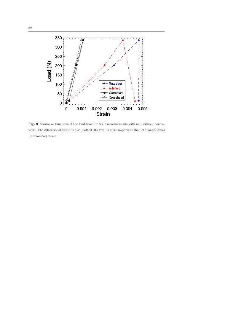
Figure 9 shows the change of strains as a function of the applied load. Without

correction, the longitudinal strain εkk is significantly overestimated due to dilatational

effects. Further, the dilatational strain does not depend on the applied load but on

time and its effect is thus increasing during the test. This trend is consistent with the

observations of Section 4 (Figure 3). After correction of this artifact, there is a very good

agreement between the corrected strain and that derived from the global measurements

(based upon the crosshead stroke). With the eigen strains of the corrected strain tensor

ε1 ≤ ε2 < ε3, the identified value of Poisson’s ratio is ν = −(ε1+ε2)/2ε3 = 0.27, which

17

is consistent with the known value of 0.28 [38]. Young’s modulus is found to be equal to

156 GPa in good agreement with classical values of SG cast iron (160 ± 3 GPa [38]).

8 Conclusion

X-ray computed tomography is a very powerful tool to visualize opaque materials.

When the scans are further processed to measure displacement fields using DVC, it

has been shown herein that special care should be exercised. This is particularly true

for lab equipments in which divergent beams are used.

First, if the temperature of the X-ray tube is not controlled, it may induce distance

variations that result in magnification changes and thus spurious dilatational strains

whose maximum level (here observed to be of the order of 0.4 %) impedes any quan-

titative (and therefore trustful) displacement measurement. In the present case, it was

shown that the elastic properties of a cast iron cannot be evaluated without a correction

of the displacement field. This correction was also needed when stress intensity factors

were sought in similar experiments on cracked samples [21]. In both cases, it allowed

for quantitative estimates of mechanical parameters. It should however be emphasized

that this artifact also impacts image reconstruction, although this effect has not been

considered in the present study.

Second, because of the principle of tomography, reconstruction (ring) artifacts are

observed. It was shown that they degrade the overall performance in terms of mea-

surement uncertainties whose level is close to the decivoxel range, rather than the

centipixel range when optical images are used [35,36,37]. Consequently, the identifica-

tion of elastic properties becomes more delicate, even though possible as shown herein

when analyzing a tensile test on cast iron.

Third, in lab tomographs polychromatic beams are usually used. They lead to so-

called beam hardening effects. Commercial tomographs are generally provided with

correction procedures whose details are not given to the users. In the present case, it

was shown that in terms of displacement uncertainty, there is no need to correct the

reconstructed volumes.

18

Last, to quantify all the previous effects, the procedure followed herein is generic

and can be considered as a baseline analysis to better characterize a new equipment,

or an existing one when quantitative analyses such as displacement measurements are

performed. Among the three effects studied herein, the spurious dilatational strains are

definitely the most important to correct.

Acknowledgments

This work was funded by Agence Nationale de la Recherche under the grant ANR-09-

BLAN-0009-01 (RUPXCUBE Project).

19

References

1. J. Ambrose and G. N. Hounsfield, Computerized transverse axial tomography, Br. J.

Radiol. 46 [542] (1973) 148-149.

2. G. N. Hounsfield, Computerized transverse axial scanning (tomography). 1. Description

of system, Br. J. Radiol. 46 [552] (1973) 1016-22.

3. J. Baruchel, J.-Y. Buffiere, E. Maire, P. Merle and G. Peix, X-Ray Tomography in Material

Sciences, (Hermes Science, Paris (France), 2000).

4. D. Bernard, edt., 1st Conference on 3D-Imaging of Materials and Systems 2008, (ICMCB,

Bordeaux (France), 2008.

5. O. Ludwig, M. Dimichiel, L. Salvo, M. Suery and P. Falus, In-situ Three-Dimensional

Microstructural Investigation of Solidification of an Al-Cu Alloy by Ultrafast X-ray Mi-

crotomography, Metall. Mat. Trans. A 36 [6] (2005) 1515-1523.

6. E. Maire, P. Colombo, J. Adrien, L. Babout and L. Biasetto, Characterization of the

morphology of cellular ceramics by 3D image processing of X-ray tomography, J. Eur.

Ceram. Soc. 27 (2007) 1973-1981.

7. T. Juettner, H. Moertel, V. Svinka and R. Svinka, Structure of kaoline-alumina based foam

ceramics for high temperature applications, J. Eur. Ceram. Soc. 27 (2007) 1435-1441.

8. T. J. Chotarda, A. Smith, M. P. Boncoeur, D. Fargeot and C. Gault, Characterisation

of early stage calcium aluminate cement hydration by combination of non-destructive

techniques: acoustic emission and X-ray tomography, J. Eur. Ceram. Soc. 23 (2003) 2211-

2223.

9. E. Maire, A. Fazekas, L. Salvo, R. Dendievel, S. Youssef, P. Cloetens and J. M. Letang, X-

ray tomography applied to the characterization of cellular materials. Related finite element

modeling problems, Comp. Sci. Tech. 63 [16] (2003) 2431-2443.

10. L. Babout, E. Maire, J.-Y. Buffiere and R. Fougeres, Characterisation by X-Ray com-

puted tomography of decohesion, porosity growth and coalescence in model metal matrix

composites, Acta Mater. 49 [11] (2001) 2055-2063.

11. J. Bontaz-Carion and Y.-P. Pellegrini, X-Ray Microtomography Analysis of Dynamic Dam-

age in Tantalum, Adv. Eng. Mat. 8 [6] (2006) 480-486.

12. R. Sinclair, M. Preuss, E. Maire, J.-Y. Buffiere, P. Bowen and P. J. Withers, The effect of

fibre fractures in the bridging zone of fatigue cracked Ti6Al4V/SiC fibre composites, Acta

Mater. 52 [6] (2004) 1423-1438.

13. E. Ferrie, J.-Y. Buffiere, W. Ludwig, A. Gravouil and L. Edwards, Fatigue crack propa-

gation: In situ visualization using X-ray microtomography and 3D simulation using the

extended finite element method, Acta Mat. 54 [4] (2006) 1111-1122.

20

14. J.-Y. Buffiere, E. Ferrie, H. Proudhon and W. Ludwig, Three-dimensional visualisation of

fatigue cracks in metals using high resolution synchrotron X-ray micro-tomography, Mat.

Sci. Tech. 22 [9] (2006) 1019-1024.

15. S. F. Nielsen, H. F. Poulsen, F. Beckmann, C. Thorning and J. A. Wert, Measurements of

plastic displacement gradient components in three dimensions using marker particles and

synchrotron X-ray absorption microtomography, Acta Mater. 51 [8] (2003) 2407-2415.

16. B. K. Bay, T. S. Smith, D. P. Fyhrie and M. Saad, Digital volume correlation: three-

dimensional strain mapping using X-ray tomography, Exp. Mech. 39 (1999) 217-226.

17. M. Bornert, J.-M. Chaix, P. Doumalin, J.-C. Dupre, T. Fournel, D. Jeulin, E. Maire, M.

Moreaud and H. Moulinec, Mesure tridimensionnelle de champs cinematiques par imagerie

volumique pour l’analyse des materiaux et des structures, Inst. Mes. Metrol. 4 (2004) 43-

88.

18. T. O. McKinley and B. K. Bay, Trabecular bone strain changes associated with subchon-

dral stiffening of the proximal tibia, J. Biomech. 36 [2] (2003) 155163.

19. S. Roux, F. Hild, P. Viot and D. Bernard, Three dimensional image correlation from X-Ray

computed tomography of solid foam, Comp. Part A 39 [8] (2008) 1253-1265.

20. J. Rethore, J.-P. Tinnes, S. Roux, J.-Y. Buffiere and F. Hild, Extended three-dimensional

digital image correlation (X3D-DIC), C. R. Mecanique 336 (2008) 643-649.

21. N. Limodin, J. Rethore, J.-Y. Buffiere, A. Gravouil, F. Hild and S. Roux, Crack closure

and stress intensity factor measurements in nodular graphite cast iron using 3D correlation

of laboratory X ray microtomography images, Acta Mat. 57 [14] (2009) 4090-4101.

22. J. Rannou, N. Limodin, J. Rethore, A. Gravouil, W. Ludwig, M.-C. Baıetto-Dubourg,

J.-Y. Buffiere, A. Combescure, F. Hild and S. Roux, Three dimensional experimental and

numerical multiscale analysis of a fatigue crack, Comp. Meth. Appl. Mech. Eng. 199 (2010)

1307-1325.

23. A. C. Kak and M. Slaney, Principles of computerized tomographic imaging, (IEEE Press,

New York, 1988).

24. S. R. Stock, MicroComputed Tomography: Methodology and Applications, (CRC, 2008).

25. S. R. Stock, Recent advances in X-Ray microtomography applied to materials, Int. Mat.

Rev. 53 [3] (2008) 129-181.

26. G. R. Davis and J. C. Elliot, Artefacts in X-ray microtomography of materials, Mat. Sci.

Eng. 22 [9] (2006) 1011-1018.

27. ESRF, http://www.esrf.eu/UsersAndScience/Experiments/Imaging/ID19/Software/ringcorrection,

(accessed on december 15, 2009).

28. M. L. Rivers and Y. Wang, Recent developments in microtomography at GeoSoilEnviro-

CARS, in: Developments in X-Ray Tomography V , U. Bonse, eds., (SPIE, Bellingham

Wa, 2006) 6318 0J-1-15.

21

29. R. A. Ketcham, New algorithms for ring artefact removal, in: Developments in X-Ray

Tomography V , U. Bonse, eds., (SPIE, Bellingham Wa, 2006), 6318 00-1-15.

30. P. L. Salmon, X. Liu and A. Sasov, A post scan method for correcting artefacts of slow

geometry changes during micro-tomographic scans, J. X-Ray Sci. Tech. 17 (2009) 161-174.

31. L. A. Feldkamp, L. C. Davis and J. W. Kress, Practical cone beam algorithm, J. Opt. Soc.

Am. A1 (1984) 612-619.

32. F. Hild, E. Maire, S. Roux and J.-F. Witz, Three dimensional analysis of a compression

test on stone wool, Acta Mat. 57 (2009) 3310-3320.

33. A. B. De Vriendt, La transmission de la chaleur , (Morin, Quebec (Canada), 1987).

34. G. Besnard, F. Hild and S. Roux, “Finite-element” displacement fields analysis from digital

images: Application to Portevin-Le Chatelier bands, Exp. Mech. 46 (2006) 789-803.

35. H. W. Schreier, J. R. Braasch and M. A. Sutton, Systematic errors in digital image corre-

lation caused by intensity interpolation, Opt. Eng. 39 [11] (2000) 2915-2921.

36. X. Fayolle, S. Calloch and F. Hild, Controlling testing machines with digital image corre-

lation, Exp. Tech. 31 [3] (2007) 57-63.

37. K. Triconnet, K. Derrien, F. Hild and D. Baptiste, Parameter choice for optimized digital

image correlation, Opt. Lasers Eng. 47 (2009) 728-737.

38. P. Dierickx, Etude de la microstructure et des mecanismes d’endommagement de fontes

G.S. ductiles : influence des traitements thermiques de ferritisation, (PhD dissertation,

INSA de Lyon, 1996).

22

List of Figures

1 Schematic view of the process of tomographic acquisition and recon-

struction. Ring artifacts are visible on one axial cut of the reconstructed

volume. . . . . . . . . . . . . . . . . . . . . . . . . . . . . . . . . . . . . 24

2 Norm in voxels for the measured (a) displacement after removal of rigid

body motions, the dilatational displacement (b), and the difference of

the two displacement fields (c). The region of interest is cut through its

mid-plane for visualization purposes. . . . . . . . . . . . . . . . . . . . 25

3 Change of the dilatational strain with time for three series of experiments

(a). Change of the normalized dilatational strain ε/ε∞ with time for the

three series (b). The dashed lines correspond to the interpolation by

using Equations (5) and (6). . . . . . . . . . . . . . . . . . . . . . . . . . 26

4 Change of the standard displacement uncertainty when a longitudinal

translation is prescribed to the sample. The effect of a correction ac-

counting for dilation, and rotation is compared to the raw data. The

result of the a priori analysis is shown for comparison purposes. The

curves are linear interpolations (in the log-log plot) of the various results. 27

5 Change of the standard displacement uncertainty when a transverse

translation is prescribed to the sample. The effect of a correction ac-

counting for dilation, and rotation is compared to the raw data. The

result of the a priori analysis is shown for comparison purposes. The

curves are linear interpolations (in the log-log plot) of the various results. 28

6 Correlation residuals for a longitudinal (a) and transverse (b) motion.

The ring artifacts are clearly visible, and the locations of the two rotation

axes when a transverse motion is applied. . . . . . . . . . . . . . . . . . 29

7 Illustration of beam hardening affecting image reconstruction. . . . . . . 30

23

8 Standard displacement uncertainty versus element size for raw measure-

ments and after the correction with the fields of Equation (4). The same

results are obtained with and without beam hardening corrections. The

result of the a priori analysis is shown for comparison purposes. The

curves are linear interpolations (in the log-log plot) of the various results. 31

9 Strains as functions of the load level for DVC measurements with and

without corrections. The dilatational strain is also plotted. Its level is

more important than the longitudinal (mechanical) strain. . . . . . . . 32

24

X-ray

tube

Radiographs

900 projections

DetectorSample

Rotation stage

0 -360°

3D rendering and zoom

in a slice showing rings

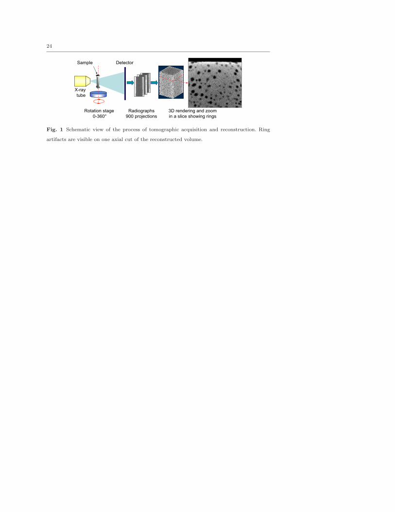
Fig. 1 Schematic view of the process of tomographic acquisition and reconstruction. Ring

artifacts are visible on one axial cut of the reconstructed volume.

25

(a) (b) (c)

Fig. 2 Norm in voxels for the measured (a) displacement after removal of rigid body motions,

the dilatational displacement (b), and the difference of the two displacement fields (c). The

region of interest is cut through its mid-plane for visualization purposes.

26

! "

#%$ &('*)+&,$ -.

(a)

! ! " #! "

$% &('*)+&, -.

(b)

Fig. 3 Change of the dilatational strain with time for three series of experiments (a). Change

of the normalized dilatational strain ε/ε∞ with time for the three series (b). The dashed lines

correspond to the interpolation by using Equations (5) and (6).

27

! " #! ! $% &' ()

*,+ -/.0-2132465 78-:9<;>=6?@-A+ B

CDFEHGDI D

JK L DI K MON

JK L DI K MONQP/R MI DI K MSN

Fig. 4 Change of the standard displacement uncertainty when a longitudinal translation is

prescribed to the sample. The effect of a correction accounting for dilation, and rotation is

compared to the raw data. The result of the a priori analysis is shown for comparison purposes.

The curves are linear interpolations (in the log-log plot) of the various results.

28

! "

#%$#%&#'# $#%&#'# $#%&#'(*)+-, .+/,

01 234 567879: ;967<: 519: => ?@ A74B CDFEHGDI D

JK L DI K MONJK L DI K MONQPR M I DI K MSN

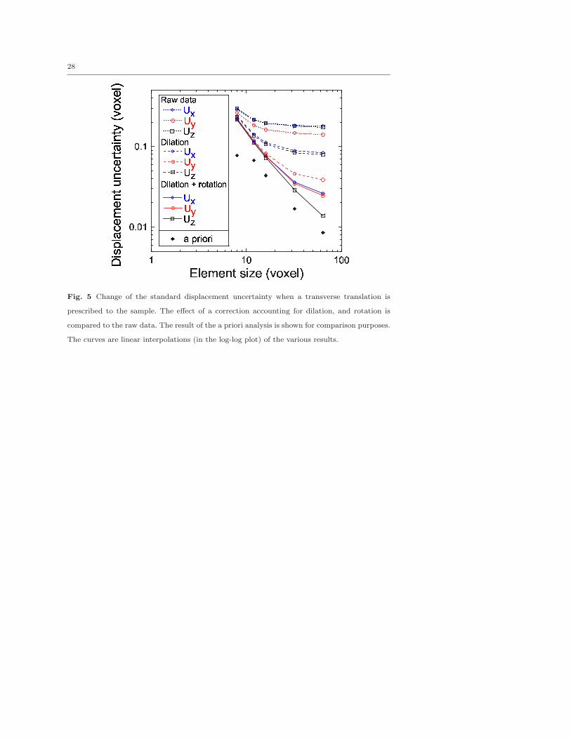
Fig. 5 Change of the standard displacement uncertainty when a transverse translation is

prescribed to the sample. The effect of a correction accounting for dilation, and rotation is

compared to the raw data. The result of the a priori analysis is shown for comparison purposes.

The curves are linear interpolations (in the log-log plot) of the various results.

29

(a) (b)

Fig. 6 Correlation residuals for a longitudinal (a) and transverse (b) motion. The ring artifacts

are clearly visible, and the locations of the two rotation axes when a transverse motion is

applied.

30

Fig. 7 Illustration of beam hardening affecting image reconstruction.

31

! "#$ %&' (%)' !' *+ ,- .$/

021 3546387:95;=< >?3A@CBEDGFG351 ;GH

IJ5KLM

KLM

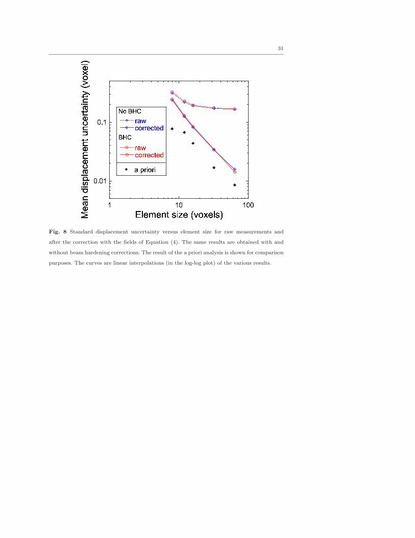
Fig. 8 Standard displacement uncertainty versus element size for raw measurements and

after the correction with the fields of Equation (4). The same results are obtained with and

without beam hardening corrections. The result of the a priori analysis is shown for comparison

purposes. The curves are linear interpolations (in the log-log plot) of the various results.

32

!"# $ " #%%&

')( *+-, .

/ 0123 45

Fig. 9 Strains as functions of the load level for DVC measurements with and without correc-

tions. The dilatational strain is also plotted. Its level is more important than the longitudinal

(mechanical) strain.