9

ANALYSING QUANTITATIVE DATA

Although, of course, there are other software packages that can be used for quantitative data analysis, including Microsoft Excel, SPSS is perhaps the one most commonly subscribed to by higher education institutions and is therefore the one most likely to be available to you to help you undertake this type of analysis. In addition to the hints, tips, advice and guidance contained within this chapter there are also valuable support resources available via both the Video and Web Link sections of the Companion Website (study.sagepub.com/brotherton) covering the use of SPSS specifically and also on more general aspects of statistical analysis.

Technique Tip

Using SPSS to Recode Data

[1] Go to the Transform menu, select ‘Recode’, then select ‘Into Different Variables’ (see the note below) to open this dialogue box.

[2] Select the variable you wish to recode from the list and move it into the ‘Numeric Variable > Output Variable’ box. Then type the name for the new variable into the ‘Output Variable/Name’ box. Click on ‘Change’ and it will be inserted in the ‘Numeric Variable > Output Variable’ box.

[3] Now you need to tell SPSS how to change the values of the original variable to the new one. To do this, click on the ‘Old and New Values’ button to open this dialogue box. There you have options to change single values or ranges of values from the original to the new variable (see the example below). Whichever option you choose, you need to enter the new value in the ‘New Value’ box and then click on the ‘Add’ button to add it to the new values list in the adjacent window.

[4] When you have entered all the old for new values, click on the ‘Continue’ button to return to the main dialogue box, and then click on ‘OK’. A new variable with the name you have given it will then appear in the datasheet in the Data View window.

Bob Brotherton 2015

Technique TipUsing SPSS to Format

Variables for Data Entry

[1] In the first column – ‘Name’ – type the name you wish to give the variable. This is limited to eight characters or fewer, but you will have the option later to provide a longer name or description for the variable (see 3 below).

[2] In the second column – ‘Type’ – you need to specify whether the type of data is of a numeric or string form – that is, numbers or words. The default for this is numeric. To change it to a particular type of numeric value, a string format or specify the format of the numeric value, click on the button to the right of the word ‘Numeric’. This opens the ‘Variable Type’ box, which contains these options. Assuming that you do not wish to specify a particular type, all you may wish to change are the default numbers of 8 and 2 in the ‘Width’ and ‘Decimal Places’ boxes. If you have data with more than eight digits, then you may wish to adjust this value. Similarly, if all your data are comprised of whole numbers, then you might want to set the ‘Decimal Places’ number to zero. If you make changes to any of the default values, then these will appear in the third (‘Width’) and fourth (‘Decimal Places’) columns once you have clicked on ‘OK’ and returned to the Variable View window.

[3] In the fifth column – ‘Label’ – you have the opportunity to enter a longer description for each variable, which can be useful when you produce some output. For example, the variable name might be ‘Occ’, for ‘occupation’. Here, the complete word can be entered as a fuller description to facilitate identification of the variable when output statistics are produced. To do this, simply click on the cell and type in the longer name.

Note: It is possible to recode a variable without creating a new variable by using the ‘Into Same Variable’ option but this will mean that you will lose your original data, as it will be changed into the new format.

Example: If you have a range of raw, or ungrouped, data values and wish to recode them into categories, then you will need to specify the ranges to be included in each new category. So, you might inform SPSS that the old values up to 20 should be the first category by checking the ‘Range (Lowest Through)’ option and entering 20 in that box. This will place all the values up to and including 20 into the first new category you specify. For the highest category, you follow essentially the same procedure, but use the ‘Range (Through Highest)’ option, entering the lowest value of this category. So, if you want this category to be from 70 upwards, enter ‘70’ in the box. For intermediate categories between the lowest and highest, you need to use the ‘Range (Through)’ boxes to enter the lowest and highest values for the category.

[4] The sixth column – ‘Values’ – gives you the opportunity to enter value labels, or descriptors, for the categories or scale intervals in your data. For example, in the case of the variable ‘Gender’ there will be categorical values for males and females. You may have decided to code these as 1 for males and 2 for females, but, unless you tell SPSS what the 1s and 2s mean, it will not know. Similarly, in the case of a scale, say a five-point Likert scale, you will be entering numbers between 1 and 5, but, again, SPSS will not know what these relate to unless it is told. Clicking on the right-hand side of the ‘Values’ cell will open the ‘Value Label’ box. In it you can enter the value and its corresponding label. So, from the example above, if you type ‘1’ in the ‘Value’ box and then ‘Male’ in the ‘Value Label’ box, then click on ‘Add’, this will appear in the ‘Summary’ box below as ‘1 = Male’. You then simply repeat this procedure for the remaining items until you have labelled them all, then click on ‘OK’ to return to the Variable View window. There you will see that these values are displayed in the relevant ‘Values’ cell.

[5] The seventh column – ‘Missing’ – enables you to specify how SPSS should deal with any missing values in the data. Unless you wish to provide a specific instruction to deal with missing values in a particular way, this can be ignored.

[6] The eighth column – ‘Columns’ – is used to set the width of the columns in the data sheet. The default for this is eight characters wide and this is usually sufficient. So, unless you have long numeric or string data, it is best to leave this as it is.

[7] The ninth column – ‘Align’ – sets the alignment of the data in the cells of the data sheet. The default setting is ‘Right’ and, once again, there is little to be gained by changing this, unless you have particular reasons for doing so.

[8] The final column – ‘Measure’ – enables you to specify the type of data relating to the variable. The default setting for this is ‘Scale’, which is for interval or ratio data, but this can be changed to ‘Nominal’ or ‘Ordinal’ if your data for the variable are one of these types. To make the change, simply click on the right-hand side of the cell and select the appropriate option.

Shortcuts: Once you have set up all the attributes for a variable, it is possible to save time and effort in setting up others that have either all or some of the attributes. If other variables have all the same attributes except the name and label, then you can copy and paste them to save entering all the same information again for each one.

Where you want to copy and paste all the variable’s attributes, you can do this as follows. In the Variable View, click on the row number of the variable you wish to copy the attributes from. This should highlight the whole row. Then press ‘Control-C’ to copy the information and click on the empty row you want to use for the new variable. Now press ‘Control-V’ to paste the information in. All you will have to change is the variable name and its label.

Where you only want to copy and paste the attributes from one or two cells, then you can simply select the cell(s) concerned, copy their contents, select the cell(s) you want to put this information into and paste it in.

Technique TipUsing SPSS to Split Files or

Select Cases

Splitting files

Splitting files enables you to repeat an analysis for all the categories or groups within a variable.

[1] In the Data View go to the Data menu and select the ‘Split File’ option.

[2] In the ‘Split File’ dialogue box, your list of variables will be displayed in the left-hand window. Select which one(s) you wish to use to split the file and move these to the window headed ‘Groups Based On’.

[3] From the three options above this box, if you click on ‘Compare Groups’ this will produce the groups’ results together, or, if you click on ‘Organise Output by Groups’, the results for each group will be presented separately and successively.

[4] Click on ‘OK’ to return to the Data View window.

Selecting cases

Where you wish to select particular values for your variable or categories rather than repeating the same analysis for all the variable’s categories, then this option will enable you to do exactly that.

[1] Go to the Data menu and click on the ‘Select Cases’ option.

[2] In the ‘Select Cases’ dialogue box, there are various options to specify the basis on which the cases should be selected, but perhaps the most commonly used one is the ‘If’ option. Selecting this opens the ‘If’ dialogue box for you to specify the conditions to be used to select the cases.

[3] To inform SPSS which variable the cases are to be selected from, highlight this in the left-hand window and press the button to move it into the window at the top of the ‘If’ dialogue box. Now you have to specify the condition or value of the variable to be used to select the cases. This can be done using the keypad or ‘Functions’ options below the window. For example, if you only want the analysis to apply to the category of male respondents and this has previously been coded as 1, from the variable ‘Gender’, then you need to set the window as ‘gender = 1’. It is also possible to set the condition to include more than one category for selecting the cases using the ‘And’ or ‘Or’ operators.

[4] Once the condition has been set, click on ‘Continue’ to return to the ‘Select Cases’ dialogue box, then click ‘OK’ to return to the Data View window.

Note: When you return from the ‘Split File’ or ‘Select Cases’ boxes, you will see that changes have occurred to the organisation of your data in the data sheet and, in the bar at the bottom of the screen, either the words ‘Split File on’ or ‘Filter on’ will be displayed, respectively. These changes are not permanent, but once you have completed the analysis for the split file or selected cases you need to turn off the function, otherwise any further analyses will only be conducted on this basis.

To turn off the split file and return the data sheet to a normal format, go to the Data menu, select ‘Split File’, click on the first option – ‘Analyse all cases, do not create groups’ – and click on ‘OK’. To turn off select cases, go to the Data menu, choose ‘Select Cases’, click on the ‘All cases’ option, then Click on ‘OK’. You can tell when these options are switched on or off by looking at the display in the status bar at the bottom of the Data View window.

Technique TipUsing SPSS to Obtain

Frequency Distributions/Tables

[1] Go to the Analyse menu, select ‘Descriptive Statistics’, then ‘Frequencies’.

[2] In the ‘Frequencies’ dialogue box, select the name(s) or number(s) you have given to the variable(s) you wish to see the frequencies for and press the arrow key to place these in the ‘Variables’ window.

[3] If you then click on ‘OK’, without changing the other options available, SPSS will do the calculations and display these as tables in an ‘Output’ window that you can save as a separate file using the ‘Save As’ command.

Technique TipUsing SPSS to Produce Charts

and Graphs

[1] In SPSS you can do this quite easily by going to the Graphs menu and selecting the type of chart you wish to produce. There you will be given the options to produce bar or pie charts, histograms, line graphs and other types of chart.

[2] Selecting one of these will open the appropriate dialogue box for you to specify the variable to be charted or graphed and the format for this.

[3] You can also produce bar and pie charts and histograms at the same time as you request frequencies from within the ‘Frequencies’ dialogue box. Having selected the variable(s) you wish to chart, click on the ‘Charts’ button, select the desired type in the options box this opens, click on ‘Continue’ to return to the ‘Frequencies’ box and click on ‘OK’ to activate the process.

Technique Tip Using SPSS to Obtain Measures of Central Tendency, Dispersion

and Skewness

[1] Go to the Analyse menu, select ‘Descriptive Statistics’, then ‘Descriptives’.

[2] In the ‘Descriptives’ dialogue box, you then need to place the variables you wish to have these measures calculated for into the ‘Variables’ box.

[3] Click on the ‘Options’ button, select the statistics you require, then click on ‘Continue’ to return to the ‘Descriptives’ box.

[4] Click on ‘OK’ and the results will then appear in an ‘Output’ window.

Note: The interpretation of these results should be straightforward, but if you have selected ‘Skewness’ and/or ‘Kurtosis’ to get a feel for the shape of the data distribution, these may not be so familiar.

Skewness provides an indication of how symmetrical the distribution is and kurtosis how peaked or flat it is. If the distribution is normal, both of these will have a value of zero. A positive skewness value would indicate a clustering of data to the left of the distribution, while a negative value would be the reverse of this. Kurtosis values that are positive indicate the distribution is peaked and those that are negative indicate a flatter distribution.

Research inAction

Expressing Sample Representativeness

The size of the realised sample (n = 239) was very encouraging in terms of providing a representative data set from the budget hotel sector. Not unsurprisingly, it was dominated by the two leading brands Premier Travel Inn (originally Travelinn, now Premier Inn) and Travelodge. Though this did skew the sample in favour of these brands, this nevertheless reflects the population distribution of budget hotel brands in the UK.

The sample was also dominated by budget hotels in motorway and A (trunk road) road locations, with these accounting for almost two-thirds of the respondent hotels. However, this again reflects the nature of the population distribution for budget hotel locations. Interestingly, the more recent growth locations of suburban and city centre sites also feature quite strongly, accounting for nearly a further 30 per cent of the sample.

The size distribution shows the 31–40 bedroom range to be the largest single category, followed by the over 60 bedroom group. Cumulatively these two size categories account for 74 per cent of the total. If the 41–50 category were to be added to these, this would account for some 90 per cent of the total. Once again, this is strongly representative of the budget hotel population distribution by size.

Other categorical data also indicates that the sample is very representative of the breadth of budget hotel operations, as this is comprised of a considerable range of responses in relation to average room occupancy, number of full- and part-time staff and the business mix. Given all of these characteristics it is reasonable to claim that the sample as a whole is highly representative of branded budget hotel operations in the UK.

Source: Brotherton (2004). 949–50 Reproduced with permission from Emerald Group Publishing Limited

Technique TipUsing SPSS to Calculate

Split-Half Reliability

[1] Go to the Analyse menu, select ‘Scale’ and then ‘Reliability Analysis’.

[2] Select all the variables that are included in the set or scale and move these into the ‘Items’ box.

[3] Select ‘Alpha’ in the ‘Models’ section of the box.

[4] Click on the ‘Statistics’ button and select ‘Item, Scale and Scale If Item Deleted’ in the ‘Descriptives For’ section. Click on ‘Continue’ to return to the ‘Reliability Analysis’ box.

[5] Click on ‘OK’ and the results will appear in an ‘Output’ window.

Note: This can produce a lot of data, especially if there are many items included in the scale, but the key results to examine are as follows. First, at the end of the output, there will be a figure for the alpha value. This is the Cronbach’s alpha coefficient and it indicates the internal consistency or coherence of the set of items. It is the sum of all the correlations between the items and, the closer it is to 1 (remember, a correlation coefficient of 1 indicates a perfect correlation), the greater the relatedness or consistency of the set of items.

It is generally accepted that, for the scale to be considered reliable, the alpha value should be at least 0.7, with higher values moving towards 1 indicating greater reliability. If the alpha value is less than 0.7, then you may be able to improve it by removing items that have a low correlation with others in the set. The column headed ‘Alpha if Item Deleted’ will indicate what the alpha value would be if an item was deleted from the scale. If, when doing this for any of the items, it shows that the overall alpha value would be higher than 0.7 if it were to be removed, then you may wish to consider doing this. You can also examine such a column even if the alpha is 0.7 or greater to see if it could be improved by removing any of the items.

However, you need to be careful because you may find that removal of one or more items only improves the alpha value by a very small amount, which may not be a price you are prepared to pay to gain a small increase in reliability. In other words, some of the items may have already been found to be statistically significant and removing these would involve trading off some validity for greater reliability.

Technique TipUsing SPSS to Produce

Cross-Tabulation Results

[1] Go to the Analyse menu, select ‘Descriptive Statistics’, then ‘Crosstabs’ to open this dialogue box.

[2] There, you need to select the dependent and independent variables from the list of variables in the box on the left. This is done by specifying which variables are to be used for the rows and which for the columns of the table. You can choose to enter the dependent variables in either the rows or the columns, but it may be preferable to enter the independent variables in the rows and the dependent variables in the columns. This is done by simply selecting the appropriate variable from the list and pressing the relevant arrow key to place it in either the ‘Rows’ or ‘Columns’ boxes.

[3] Once you have completed this task, click on the ‘Cells’ button and check the ‘Row’ and ‘Total’ boxes in the ‘Percentages’ section to ensure that the percentages are calculated by rows – the independent variables. If you have decided to place the independent variables in the columns of the table, then, of course, you need to check the ‘Columns’ box.

[4] Click on ‘Continue’, then, when the display has returned to the ‘Crosstabs’ dialogue box, click on ‘OK’ and the results will appear in an ‘Output’ window.

Technique Tip

Using SPSS to Produce Scatter Graphs

[1] Go to the Graphs menu and select ‘Scatter’. In the dialogue box, ensure that ‘Simple’ is highlighted and click on the ‘Define’ button.

[2] From the list of variables displayed, select the one you wish to be the independent variable and add this to the X-axis box, and then do the same for the dependent variable, adding this to the Y-axis box.

[3] If you wish to add titles and labels to the graph, you can do this using the ‘Titles’ button. Click on ‘OK’ to activate the calculation and open the output window containing the scatter graph.

Technique TipUsing SPSS to Produce Correlation Coefficients

[1] Go to the Analyse menu, select ‘Correlate’ and then ‘Bivariate’(for two variables).

[2] In the dialogue box, select the two variables to correlate, add these to the ‘Variables’ box, and then select the appropriate correlation calculation – either Pearson’s or Spearman’s – in the ‘Correlation Coefficients’ section (see the note below). Also at this point select the ‘2 Tail’ box, unless you have good reasons to support the view that the correlation will take a specific direction, in which case you can choose the ‘1 Tail’ option.

[3] Next, click on the ‘Options’ button and, in the window that opens, select ‘Exclude Cases Pairwise’ under ‘Missing Values’. If you wish to include the means and standard deviations in the output, then you can also select those there.

[4] Click on ‘Continue’ and then ‘OK’ when you return to the previous window to produce the results in an ‘Output’ window.

Note: If all of your data are of the interval or ratio kind, then the preferred choice of correlation coefficient should be Pearson’s product moment correlation coefficient. However, this does assume that the data for both variables are normally distributed. If they are not, or any of your data are ordinal or ranked, then choose the Spearman’s rank correlation coefficient. Both methods produce the same type of output, but they may not produce the same value for the coefficient!

Technique TipUsing SPSS to Obtain the

Chi-Square Test for Independence

[1] Go to the Analyse menu, then ‘Descriptive Statistics’ and select ‘Crosstabs’.

[2] In the ‘Crosstabs’ dialogue box, select and move your variables into the ‘Rows’ and ‘Columns’ boxes.

[3] Next, click on the ‘Statistics’ button, select ‘chi-square’ and then click on ‘Continue’ to return to the ‘Crosstabs’ dialogue box.

[4] Now, click on the ‘Cells’ button and, in the ‘Counts’ box, click on the ‘Observed’ and ‘Expected’ options. In the ‘Percentage’ section, click on ‘Column, Row and Total’. Click on ‘Continue’ and then ‘OK’ after returning to the ‘Crosstabs’ dialogue box.

[5] The results will now appear in an ‘Output’ window.

Technique TipUsing SPSS to Produce Simple

(Two Variable) Regression Analysis

[1] Go to the Analyse menu, select ‘Regression’ and then ‘Linear’.

[2] In the ‘Linear Regression’ dialogue box, select and move the independent and dependent variables into the respective boxes.

[3] Before clicking on ‘OK’ to produce the regression results, it is possible to request other statistics by pressing the ‘Statistics’ button. In the box this opens, a range of options is available, but unless you are very familiar with regression analysis, it may be advisable to select only ‘Estimates’, ‘Model Fit’ and ‘Descriptives’. You may also wish to select ‘Casewise Diagnostics’ and set the ‘Outliers’ value to 3 standard deviations in the ‘Residuals’ section (see the note below).

Note: The ‘Casewise Diagnostics’ option allows you to identify whether or not there are any very large residuals or outliers that could be eliminated from the analysis to improve it.

TABLE 9.1 Parametric and non-parametric tests for confirmatory analysis

Parametric (P) and non-parametric (NP) tests Type of data Purpose

Confidence intervals (P) Normally distributed univariate

Estimating from samples

Pearson’s product moment correlation coefficient (P)

Bivariate (interval or ratio data)

Measuring association and exploring relationships

Spearman’s rank order correlation coefficient (NP)

Bivariate (at least ordinal data)

Measuring association and exploring relationships

Independent samples t-tests (P)(NP equivalent is the Mann–Whitney U test)

Bivariate (at least interval data for the dependent variables)

Measuring difference and comparing independent groups

Paired samples t-test (P)(NP equivalent is the Wilcoxon signed-rank test)

Bivariate (at least interval data for the dependent variables)

Measuring difference and comparing the same subjects on more than one occasion

One sample t-test (P) Bivariate (at least interval data)

Measuring difference and comparing the sample subjects to a test value

Chi-square test for independence (NP)

Bivariate (nominal data) Measuring difference and comparing groups

Chi-square test for goodness of fit (NP)

Bivariate (nominal data) Measuring difference and comparing groups

Technique TipUsing SPSS to Conduct

Student’s t-Tests

Independent Samples t-Tests

These tests are used to compare the mean score, from a continuous variable, with two separate groups of sample subjects.

[1] Go to the Analyse menu and click on ‘Compare Means’, then select ‘Independent samples t-test’.

[2] In the dialogue box that opens, select the dependent variable – the continuous variable – from the list of variables in the box on the left and click on the button to move this into the ‘Test Variable(s)’ box.

[3] Next, select the independent variable from the list and click on the button to move this into the ‘Grouping Variable’ box.

[4] Then click on ‘Define Groups’ to enter the numbers used to code each group in the data file. For example, if the variable were ‘Gender’ and 1 = males and 2 = females, then you would enter 1 in the ‘Group 1’ box and 2 in the ‘Group 2’ box. Click on ‘Continue’.

[5] Back in the main dialogue box, you will now see the two group numbers in brackets after the name of the variable in the ‘Grouping Variable’ box – in our example, ‘Gender (1 2)’. Click on ‘OK’ to produce the results.

Note: In the output for this test, you need to examine the significance (sig.) figure for Levene’s test for equality of variances first. This examines whether the variation in scores across the two groups is the same. If the sig. figure for this is greater than 0.05, which indicates no significant difference, then the ‘Equal Variances Assumed’ results can be used. If it is less than 0.05, then this assumption is not valid and the ‘Equal Variances Not Assumed’ results should be used. In both cases, the ‘Sig. Two-Tailed’ column is the one you are interested in as the result there shows whether there is a significant difference (p <0.05) between the groups or not (p >0.05).

Paired Samples t-Tests

These tests are also sometimes referred to as ‘repeated measures’ tests and are used where you have two samples from exactly the same respondents – that is, when you have collected data from them on two separate occasions or under different conditions. For example, in an experiment where a pre-test is undertaken before any ‘treatment’ is applied and where a post-test occurs after the treatment.

[1] Go to the Analyse menu, click on ‘Compare Means’ and then ‘Paired Samples t-test’.

[2] Click on the two variables you wish to use for the analysis in the left-hand box and these will appear, highlighted, in the ‘Current Selections’ area under the variables list box.

[3] Click on the button to place these into the ‘Paired Variables’ box on the right, then click on ‘OK’ to produce the results.

Note: The table entitled ‘Paired Samples Test’ is the one you are interested in. In the final column of this, labelled ‘Sig. (Two-tailed)’, you have the p values to indicate whether the test has found any statistically significant differences between the two variables (p <0.05) or not (p >0.05). To establish the nature of this difference, examine the ‘Mean’ scores for the two variables in the ‘Paired Samples Statistics’ table.

One Sample t-Tests

These are used to test the confidence interval for the mean of a single population. Here, as there is only one sample and one mean, we do not have other sample means to make comparisons with, but this is dealt with by establishing a test value to represent another mean.

[1] Go to the Analyse menu, click on ‘Compare Means’ and then ‘One Sample t-test’.

[2] In the dialogue box that opens, select from the list of variables in the box on the left the variable you wish to use for the test and click on the button to move this into the ‘Test Variable(s)’ box.

[3] In the ‘Test Value’ box, enter the figure to be used as the comparator for your variable’s mean. For example, if the variable had scores based on a 1–5 scale, the null hypothesis could be rejected if this was very close to the ‘indifference’ point in this scale of 3. Therefore, in this case, to establish if the data indicate that you can reject the null hypothesis, you set the ‘Test Value’ to 3 so that the mean of the variable is compared to it to establish whether it is significantly different or not.

[4] Click on ‘OK’ to produce the results.

Note: The most important figure in these results is the sig. two-tailed figure in the one sample test table. If it is >0.05, then the difference between the variable’s mean and the test value is not statistically significant and the null hypothesis cannot be rejected and vice versa.

TABLE 9.2 Summarised one sample t-test results

Critical success factors Mean SD

1 Central sales/reservation system 4.13 0.82 2 Convenient locations 4.43 0.65 3 Standardised hotel design 3.81 0.90 4 Size of hotel network 3.92 0.90 5 Geographic coverage of hotel network 4.09 0.81 6 Consistent accommodation standards 4.76 0.43 7 Consistent service standards 4.75 0.50 8 Good-value restaurants 4.03 0.81 9 Value for money accommodation 4.68 0.5710 Recognition of returning guests 4.43 0.6911 Warmth of guest welcome 4.71 0.5212 Operational flexibility/responsiveness 4.05 0.7513 Corporate contracts 3.12 1.214 Smoking and non-smoking rooms 4.14 0.8515 Design/look of guest bedrooms 3.99 0.7916 Size of guest bedrooms 3.77 0.8317 Guest bedrooms’ comfort level 4.33 0.6918 Responsiveness to customers’ demands 4.42 0.6419 Customer loyalty/repeat business 4.56 0.6020 Disciplined operational controls 4.13 0.7621 Speed of guest service 4.35 0.6922 Efficiency of guest service 4.50 0.6023 Choice of room type for guests 3.71 0.9224 Guest security 4.46 0.7125 Low guest bedroom prices 3.79 0.9526 Limited service level 3.07 1.027 Hygiene and cleanliness 4.86 0.3728 Quality audits 4.23 0.8729 Staff empowerment 3.91 0.8830 Strong brand differentiation 4.08 0.9031 Customer surveys/feedback 4.08 0.9232 Staff training 4.74 0.4733 Added-value facilities in guest rooms 3.55 1.034 Staff recruitment and selection 4.27 0.7235 Standard pricing policy 4.11 0.8836 Quality standards 4.73 0.56

Note: All the CSFs are significant, in a positive direction, at the p <0.001 level, except factors 13 (Corporate contracts) and 26 (Limited service level), which are not significant.

Source: Brotherton (2004: 952). Reproduced with permission of Emerald Publications

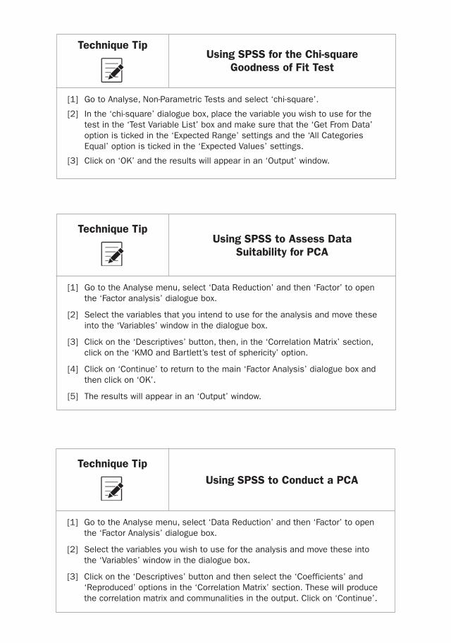
Technique TipUsing SPSS for the Chi-square

Goodness of Fit Test

[1] Go to Analyse, Non-Parametric Tests and select ‘chi-square’.

[2] In the ‘chi-square’ dialogue box, place the variable you wish to use for the test in the ‘Test Variable List’ box and make sure that the ‘Get From Data’ option is ticked in the ‘Expected Range’ settings and the ‘All Categories Equal’ option is ticked in the ‘Expected Values’ settings.

[3] Click on ‘OK’ and the results will appear in an ‘Output’ window.

Technique TipUsing SPSS to Assess Data

Suitability for PCA

[1] Go to the Analyse menu, select ‘Data Reduction’ and then ‘Factor’ to open the ‘Factor analysis’ dialogue box.

[2] Select the variables that you intend to use for the analysis and move these into the ‘Variables’ window in the dialogue box.

[3] Click on the ‘Descriptives’ button, then, in the ‘Correlation Matrix’ section, click on the ‘KMO and Bartlett’s test of sphericity’ option.

[4] Click on ‘Continue’ to return to the main ‘Factor Analysis’ dialogue box and then click on ‘OK’.

[5] The results will appear in an ‘Output’ window.

Technique TipUsing SPSS to Conduct a PCA

[1] Go to the Analyse menu, select ‘Data Reduction’ and then ‘Factor’ to open the ‘Factor Analysis’ dialogue box.

[2] Select the variables you wish to use for the analysis and move these into the ‘Variables’ window in the dialogue box.

[3] Click on the ‘Descriptives’ button and then select the ‘Coefficients’ and ‘Reproduced’ options in the ‘Correlation Matrix’ section. These will produce the correlation matrix and communalities in the output. Click on ‘Continue’.

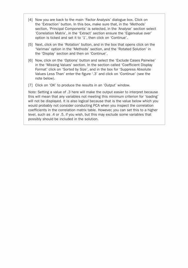
[4] Now you are back to the main ‘Factor Analysis’ dialogue box. Click on the ‘Extraction’ button. In this box, make sure that, in the ‘Methods’ section, ‘Principal Components’ is selected, in the ‘Analyse’ section select ‘Correlation Matrix’, in the ‘Extract’ section ensure the ‘Eigenvalue over’ option is ticked and set it to ‘1’, then click on ‘Continue’.

[5] Next, click on the ‘Rotation’ button, and in the box that opens click on the ‘Varimax’ option in the ‘Methods’ section, and the ‘Rotated Solution’ in the ‘Display’ section and then on ‘Continue’.

[6] Now, click on the ‘Options’ button and select the ‘Exclude Cases Pairwise’ in the ‘Missing Values’ section. In the section called ‘Coefficient Display Format’ click on ‘Sorted by Size’, and in the box for ‘Suppress Absolute Values Less Than’ enter the figure ‘.3’ and click on ‘Continue’ (see the note below).

[7] Click on ‘OK’ to produce the results in an ‘Output’ window.

Note: Setting a value of .3 here will make the output easier to interpret because this will mean that any variables not meeting this minimum criterion for ‘loading’ will not be displayed. It is also logical because that is the value below which you would probably not consider conducting PCA when you inspect the correlation coefficients in the correlation matrix table. However, you can set this to a higher level, such as .4 or .5, if you wish, but this may exclude some variables that possibly should be included in the solution.