analisis triulanan peremangan moneter … santoso, shinta r.i. soekro, darmansyah, hilde d. sihaloho...
TRANSCRIPT

1ANALISIS TRIWULANAN: Perkembangan Moneter, Perbankan dan Sistem Pembayaran, Triwulan II - 2007
BULLETIN OF MONETARY ECONOMICS AND BANKING
Center for Central Banking Research and EducationBank Indonesia
PatronDewan Gubernur Bank Indonesia
Board of Editor
Prof. Dr. Anwar NasutionProf. Dr. Miranda S. Goeltom
Prof. Dr. InsukindroProf. Dr. Iwan Jaya Azis
Prof. Iftekhar HasanProf. Dr. Masaaki Komatsu
Dr. M. SyamsuddinDr. Perry Warjiyo
Dr. Iskandar Simorangkir Dr. Solikin M. JuhroDr. Haris Munandar
Dr. Andi M. Alfian ParewangiDr. M. Edhie Purnawan
Dr. Burhanuddin AbdullahDr. Andi M. Alfian Parewangi
Editorial Chairman
Dr. Perry Warjiyo
Managing EditorDr. Darsono
Dr. Siti AstiyahDr. Andi M. Alfian Parewangi
SecretariatIr. Triatmo Doriyanto, M.S
Nurhemi, S.E., M.ATri Subandoro, S.E
This bulletin is published by Bank Indonesia, Center for Central Banking Research and Education. Contents and results research in the writings in this bulletin entirely the responsibility of the authors and not an official view of Bank Indonesia.
We invite all parties to write in this bulletin paper delivered in the form files to Center for Central Banking Research and Education, Bank Indonesia, Tower Sjafruddin Prawiranegara Floor 21; Jl. M.H. Thamrin No. 2, Central Jakarta, email: [email protected]
The Bulletin is published quarterly in April, July, October and January, for who wish to obtain this publication can contact the Dissemination Unit - Dissemination Division Statistics and Management Intern, Department of Statistics, Bank Indonesia, Tower Sjafruddin Prawiranegara floor 2; Jl. M.H. Thamrin No. 2, Central Jakarta, tel. (021) 2981-8206. For request subscribe: tel. (021) 2981-6571, fax. (021) 3501912.

Quarterly Outlook on Monetary, Banking, and Payment System In Indonesia:
Quarter III, 2014
TM. Arief Machmud, Syachman Perdymer, Muslimin Anwar, Nurkholisoh Ibnu Aman,
Tri Kurnia Ayu K, Anggita Cinditya Mutiara K, Illinia Ayudhia Riyadi
The Determining Factors Of Currency Redenomination Success:
Experimental And Historical Aproach
Andika Pambudi, Bambang Juanda, D.S. Priyarsono
Foreign Exchange Expectations in Indonesia: Regime Switching Chartists &
Fundamentalists Approach
Ferry Syarifuddin, Noer Azam Achsani, Dedi Budiman Hakim, Toni Bakhtiar
Asset Securitization and the Real Sector Performance:
An Alternative Source of Financing for SME’s
Wijoyo Santoso, Shinta R.I. Soekro, Darmansyah, Hilde D. Sihaloho
Determinant Of Non Performing Loan: The Case Of Islamic Bank In Indonesia
Irman Firmansyah
BULLETIN of moNETary EcoNomIcsaNd BaNkINg
Volume 17, Number 2, October 2014
153
221
133
183
251

This page intentionally left blank

133Quarterly Outlook On Monetary, Banking, And Payment System In Indonesia: Quarter III, 2014
1 Authors are researcher on Monetary and Economic Policy Department (DKEM). TM_Arief Machmud ([email protected]); Syachman Perdymer ([email protected]); Muslimin AAnwar ([email protected]); Nurkholisoh Ibnu Aman ([email protected]); Tri Kurnia Ayu K ([email protected]); Anggita Cinditya Mutiara K ([email protected]); Illinia Ayudhia Riyadi ([email protected]).
Indonesia’s economy in the third quarter of 2014 indicate that macroeconomic stability and the
financial system maintained and supported by a process of economic adjustment towards more balanced.
This condition is reflected in a declining current account deficit, subdued inflation and well managed
domestic demand, despite growth in the domestic economy which is expected to slow down. Meanwhile,
the stability of the financial system remains solid, sustained by the resilience of the banking system and
the relatively subdued performance of the financial markets. The national payment system continues to
run smoothly in supporting the economy.
Keywords: macroeconomy, monetary, economic outlook.
JEL Classification: C53, E66, F01, F41
Abstract
QUARTERLY OUTLOOK ON MONETARY, BANKING, AND PAYMENT
SYSTEM IN INDONESIA:QUARTER III, 2014
TM. Arief Machmud, Syachman Perdymer, Muslimin Anwar, Nurkholisoh Ibnu Aman, Tri Kurnia Ayu K,
Anggita Cinditya Mutiara K, Illinia Ayudhia Riyadi1
134 Bulletin of Monetary, Economics and Banking, Volume 17, Number 2, October 2014
I. GLOBAL DEVELOPMENT
The world economic recovery continues, although not in a balanced manner. Global economic recovery is still supported by the US economy which continues to improve. This is reflected in the indicators of increased production and decreased unemployment rate. US developments have strengthened the forecasts of the normalization of the Fed’s policy to mid 2015. Meanwhile, the economies of Europe and Japan slowed. China’s economy also indicates a signs of slowing. With these developments, global commodity prices would continue to decline, including the decline in world oil prices by increasing supply amid weakening demand. Regarding trade, global economic development will affect the export performance of Indonesia, with continued improvement in manufacturing exports in the midst of continued retention of primary commodities. Concerning the financial channels, the inflow of foreign capital into Indonesia is predicted to continue in spite of the volatility that is still quite high in relation to the normalization of the Fed’s policy. Bank Indonesia will continue to be aware of the various external risks to remain conducive to the Indonesian economy.
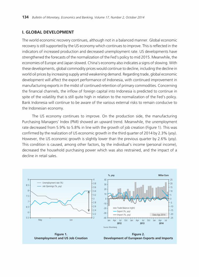
The US economy continues to improve. On the production side, the manufacturing Purchasing Managers’ Index (PMI) showed an upward trend. Meanwhile, the unemployment rate decreased from 5.9% to 5.8% in line with the growth of job creation (Figure 1). This was confirmed by the realization of US economic growth in the third quarter of 2014 by 2.3% (yoy). However, the US economic growth is slightly lower than the previous quarter by 2.6% (yoy). This condition is caused, among other factors, by the individual’s income (personal income), decreased the household purchasing power which was also restrained, and the impact of a decline in retail sales.
Figure 1.Unemployment and US Job Creation
Figure 2. Development of European Exports and Imports
������������������������������������������
���
��
�
���
�
���
���
��
��
���
�
���
��
��
���
���� ��� ��� ��� ��� ��� ��� ��� ��� ��� ��� ��� ���
���� ���� ����
���
���
���
���
�
��
��
��
��
������ �����������
���
���
���
���
��
�
�
��
��
��
��
��������������
�����������
�������������������������� ����������� ����

135Quarterly Outlook On Monetary, Banking, And Payment System In Indonesia: Quarter III, 2014
The European economy is slowing as external pressure, weakened production, and potential deflation continues. External pressure is evident by declining export growth as the Chinese economy is slowing (Figure 2). In addition, deflationary pressures and the continuing geopolitical problems of Russia still suppresses the production. This is indicated by developments in the manufacturing PMI which is in a downward trend.
The Japanese economy also experienced a slowdown driven by a weakening of production. This is indicated by the continued contraction of the production index, while at the end of the third quarter, the Japanese PMI was lower than the previous quarter. This condition is driven by the depreciation of the yen which has led to a weakening of output due to high import prices amidst limited export growth. On the other hand, demand has not improved, as indicated by department store sales that are still negative. Meanwhile, a Reuter’s survey revealed that there is deteriorating sentiment against large companies, both in manufacturing and non-manufacturing sectors. The negative sentiments are in line with the increase in the consumption tax, the increase in input prices due to the depreciation of the exchange rate, and a weakening global economy, especially China and Europe.
China’s economy is still indicating slow growth. On the demand side, the slowdown came mainly from a decline in consumption and investment growth (Figure 3). Meanwhile, in terms of production, the decline in growth mainly came from the real estate sector (tertiary industry). With these developments, the Central Bank of China (CBC) responded through a relaxation of the application rules for home loans by lowering the percentage of second home mortgages with a down payment of 30% to 60%of the house value, which came into effect the beginning of October 2014.
The Indian economy expanded and grew more than previous forecasts. The increase was driven by production activities, as indicated by the Indian PMI at a level of expansion, while the growth index showed stable production. In addition, the infrastructure index was also in an upward trend. On the domestic front, the economy indicated increasing domestic car sales and imports continue to grow. Improvements of the Indian economy are in line with the positive sentiment after the election of a new government which for example encourages the implementation of structural reforms, among others measures, in the fields of energy, infrastructure development and increase direct investment.
International trade activity decreased with the development of the global economic slowdown by major countries of the world. This is indicated by the volume of world trade which is lower than previous forecasts as well as global commodity prices that are still declining. The low growth in the world trade volume is driven by geopolitical issues and the impact of the extreme cold weather in the US in the first half that continued into the third quarter. Also, global commodity prices are still declining. The coal price decline is driven by an abundant supply and weak demand, especially from China. The weakening of the Chinese economy also decreased the price of nickel, tin, aluminum and rubber. Meanwhile, oil prices continue to decline, in line

136 Bulletin of Monetary, Economics and Banking, Volume 17, Number 2, October 2014
with the increased supply amid weak global demand. The weakening of oil prices is due to several factors, particularly fundamental factors of competition between oil producing countries and geopolitics. The fundamental factors are related to the increasing positions of the world’s oil over supply. Meanwhile, there is competition between oil producing countries encouraged by the attitude of Saudi Arabia which has no intention to reduce production amid slowing demand in order to maintain market share. Factors associated with the easing of geopolitical tensions in the Middle East and North Africa have led to a return to operation for several oil refineries in Iraq and Libya.
The global financial markets experienced a correction due to strong forecasts of implementation for the Fed’s normalization policy mid-2015. The pressure on the global financial markets was also derived from a release of the IMF related to the decline in the global economic growth which encouraged negative sentiment. Meanwhile, a majority of the global currencies weakened against the US dollar, especially Asian emerging market (EM) currencies, including the Indonesian Rupiah, which was in line with rising investor concern over global geopolitical turmoil. With these developments, the Asian stock markets continued to move up although the volume of non-resident net inflows into Asian stock markets continued to decline (Figure 4).
Figure 3.China’s Economic Growth
Figure 4.Global Stock Market Performance
��� ��� ��� ��� ��� ��� ��� ��� ��� ��� ������ ��� ��� ��� ��� ��� ��� ��� ��� ������� ���� ���� ���� ���� ����
��
�
�
��
��
����������
����� ��������������
����� ������������
��� ��� ��� ��� ��� ��� ��� ��� ��� ������� ���� ���� ���� ����
�����
��
��
���
���
���
���
���
���
���
�������
�����
���
���
���
���
��
��
����� ������ ��
� ���
����������
II. THE DYNAMICS OF Indonesia’S MACROECONOMY
2.1. Economic Growth
Along with the weak global demand, domestic economic growth tends to be moderated. Economic growth in the third quarter of 2014 is 5.01% (yoy), lower than the economic growth in the second quarter 2014 at 5.12% (yoy) (Table 1). Increased consumption is sustained by strong
137Quarterly Outlook On Monetary, Banking, And Payment System In Indonesia: Quarter III, 2014
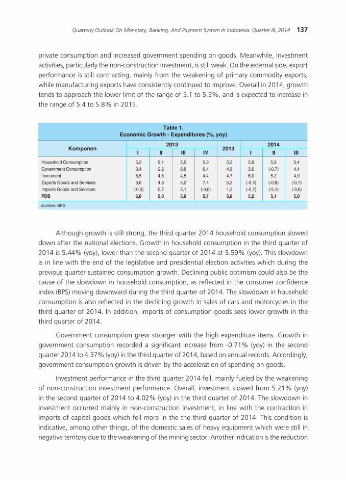
private consumption and increased government spending on goods. Meanwhile, investment activities, particularly the non-construction investment, is still weak. On the external side, export performance is still contracting, mainly from the weakening of primary commodity exports, while manufacturing exports have consistently continued to improve. Overall in 2014, growth tends to approach the lower limit of the range of 5.1 to 5.5%, and is expected to increase in the range of 5.4 to 5.8% in 2015.
Although growth is still strong, the third quarter 2014 household consumption slowed down after the national elections. Growth in household consumption in the third quarter of 2014 is 5.44% (yoy), lower than the second quarter of 2014 at 5.59% (yoy). This slowdown is in line with the end of the legislative and presidential election activities which during the previous quarter sustained consumption growth. Declining public optimism could also be the cause of the slowdown in household consumption, as reflected in the consumer confidence index (BPS) moving downward during the third quarter of 2014. The slowdown in household consumption is also reflected in the declining growth in sales of cars and motorcycles in the third quarter of 2014. In addition, imports of consumption goods sees lower growth in the third quarter of 2014.
Government consumption grew stronger with the high expenditure items. Growth in government consumption recorded a significant increase from -0.71% (yoy) in the second quarter 2014 to 4.37% (yoy) in the third quarter of 2014, based on annual records. Accordingly, government consumption growth is driven by the acceleration of spending on goods.
Investment performance in the third quarter 2014 fell, mainly fueled by the weakening of non-construction investment performance. Overall, investment slowed from 5.21% (yoy) in the second quarter of 2014 to 4.02% (yoy) in the third quarter of 2014. The slowdown in investment occurred mainly in non-construction investment, in line with the contraction in imports of capital goods which fell more in the the third quarter of 2014. This condition is indicative, among other things, of the domestic sales of heavy equipment which were still in negative territory due to the weakening of the mining sector. Another indication is the reduction
Table 1.Economic Growth - Expenditures (%, yoy)
Komponen2013
I II III IV I II III
20142013
Household Consumption 5,2 5,1 5,5 5,3 5,3 5,6 5,6 5,4Government Consumption 0,4 2,2 8,9 6,4 4,9 3,6 (-0,7) 4,4Invesment 5,5 4,5 4,5 4,4 4,7 6,0 5,2 4,0Exports Goods and Services 3,6 4,8 5,2 7,4 5,3 (-0,4) (-0,8) (-0,7)Imports Goods and Services (-0,0) 0,7 5,1 (-0,6) 1,2 (-0,7) (-5,1) (-3,6)PDB 6,0 5,8 5,6 5,7 5,8 5,2 5,1 5,0
Sumber: BPS

138 Bulletin of Monetary, Economics and Banking, Volume 17, Number 2, October 2014
in the production capacity utilization rates in the industry that shows a lack of incentives for businesses to invest. As the non-construction investment slowed down, similarly construction investment also slowed. In accordance with the historical trend, this condition is caused by the behavior of “wait-and-see” by investors during the election. Indications of a slowdown in construction investment is also reflected in slowing sales of cement and building materials imports in the third quarter 2014.
On the external side, export performance is still contracting. Exports in the third quarter of 2014 record a growth of -0.70% (yoy), slightly better than growth in the previous quarter at -0.76% (yoy). Export performance is still contracted, particularly in the export of primary commodities, due to weak global demand (Figure 5). Though still contracting, exports recorded improvement. This was driven by manufacturing exports which are still positive and the beginning realization of natural resources (mining) exports, in particular mineral concentrate exports (Figure 6).
The response of the limited performance of exports and non-construction investment is a third quarter 2014 import contraction. Imports again experience a smaller contraction from -5.05% (yoy) in the second quarter of 2014 to -3.63% (yoy) in the third quarter of 2014. On closer examination, the contraction occurred in the group of capital goods imports in line with the weakening of non-construction investments. Meanwhile, imports of consumer goods still contracted due to reduced imports of passenger cars, durable goods, and nondurable goods. In contrast, imports of raw materials grew positively, among others, in the form of foodstuffs (raw and processed) for industry, raw materials for industry, and fuel for industrial machinery.
Figure 5.World Trade Volume (Imports)
Figure 6.Real non-oil export growth
����
��������������������������� ���
� � �� ������ ���� ����
������
��
�
�
�
�
�
�
������������ �����
��������� ������� ���������
� � �� �� � � �� �� � � �� �� �� �� ���� ������ ����
�����������
���
���
���
���
�
��
��
��
��
��
���� ����
������
����
�����������
�����
�� �� ��

139Quarterly Outlook On Monetary, Banking, And Payment System In Indonesia: Quarter III, 2014
By sector, the slowing economic growth in the third quarter of 2014 is derived from lower growth in the manufacturing sector and nontradables sectors. The manufacturing sector growth slowed with weakening domestic demand and limited export performance. The slowdown is mainly in the sub-sectors of food, beverages and tobacco, chemical subsector, and the cement subsector. The building sector also contracted due to the behavior of wait-and-see businessmen to invest during the election. Trade, hotels and restaurants slowed due to the retention of international trade activity and the reduced effects of the election of previous quarter. Although growth is still high, the transport and communications sector grew less than the previous quarter at the close of the election campaign. Meanwhile, the slowdown in the financial sector, leasing, and services occurred with slowing credit growth. On the other hand, agriculture and mining growth increased compared to the previous quarter. An increase in the agricultural sector comes from the increasing growth of the food crops subsector mainly corn and soybeans. The mining sector contracted in the first quarter and the second in 2014 due to delays in mineral exports, however it bounced back with positive growth with the implementation of the Mining Law.
Regional and national economic slowdown came mainly from the weakening of economic growth in Sumatra. In addition to Sumatra, the national economic slowdown is driven by the economic slowdown that occurred in Jakarta and a contraction in NTB. The economic slowdown in Sumatra, is driven by a decline in commodity exports. Jakarta’s economy also slowed due to a slowdown in the construction sector. Meanwhile, NTB contracted significantly due to a decline in mining sector performance. On the other hand, economic growth in the region increased
Picture 1.Map of Regional Economic Growth Third Quarter 2014
gPDRB > 7% 5% < gPDRB < 6% 4% < gPDRB < 5% gPDRB Negative6% < gPDRB < 7% gPDRB < 4%
ACEH2.7
SUMUT5.3
RIAU1.7
KEP. BABEL4.6
DKI JAKARTA6 JATENG
5.4
SULTENG6.6
KALTIM3.2
KALBAR4.5
SULUT7
MALUT5.9
PAPBAR6.4
PAPUA4.1
BALI6.5 NTT
KEP. RIAU6.9
LAMPUNG5.6
BENGKULU5.1
BANTEN5
SULSEL6.2
SULBAR10
JABAR5.6 JATIM
5.9NTB
KALTENG5.5
KALSEL4.8
GORONTALO7.8
MALUKU7.3
SULTRA7.7
SUMSEL4.3
JAMBI6.6
DIY4.0
SUMBAR5.0
SUMATERA
I II III I II IIIIV2013 2014
4.54.95.4
876543
%, yoy
JAKARTA
I II III I II IIIIV2013 2014
4.04.14.0
876543
%, yoy
JAWA (Excl. Jkt)
I II III I II IIIIV2013 2014
5.65.65.7
876543
%, yoy
KTI
I II III I II IIIIV2013 2014
5.14.94.7
876543
%, yoy
NASIONAL
I II III I II IIIIV2013 2014
5.05.15.2
876543
%, yoy

140 Bulletin of Monetary, Economics and Banking, Volume 17, Number 2, October 2014
in line with the East Region of Indonesia’s (KTI) export of mineral commodities. Meanwhile, the economy of the Java (besides Jakarta) remained relatively high and with stable growth in line with the continued improvement in manufacturing exports as a result of the US economic recovery (Picture 1).
In line with the slowdown of economic growth, the unemployment rate in August 2014 increased. In August 2014, the unemployment rate stood at 5.94%, higher than in February 2014 which amounted to 5.70%. This increase was driven by a decrease in the employment rate. This decreased uptake corresponds with the slowdown in the manufacturing sector, transport and communications, finance and services sector, among others. Meanwhile, the absorption of labor in the agricultural sector tends to be stable, even uptake in the building sector and trade actually increased.
2.2. Indonesia’s Balance of Payments
Indonesia’s balance of payments (BOP) showed better performance in line with a process towards a more balanced and sustainable economic adjustment. Overall, the balance of payments in the third quarter of 2014 has a surplus of 6.5 billion US dollars, an increase of 4.3 billion dollars in the previous quarter (Figure 7). An improved balance of payments surplus is mainly driven by a decreased current account deficit compared to the previous quarter. An increase in the balance of payments surplus in turn pushed up the foreign exchange reserve from 107.7 billion US dollars at the end of the second quarter of 2014 to 111.2 billion US dollars by the end of the third quarter of 2014. The amount of the reserve is sufficient to finance payments for imports and government foreign debt for 6.3 months, and is adequate by international standards (Figure 8).
Figure 7.Indonesia’s Balance of Payments
Figure 8.Development of Reserves
�����������
�� �� �� �� �� �� �� �� �� �� �� �� ���� ���� ����������
������
������
�����
����
����
�����
�����
���� ���� ����� ����
���������� �����������������������������������������������
��� ��� ��� ��� ��� ��� ��� ��� ��� ��� ��� ��� ��� ��� ��� ��� ��� ��� ��� ������ ��� ���
�����������
���� ���� ���� ����
��
��
���
���
� �
���
�
�
�
�
������������������������������������ ��������������� ���������
141Quarterly Outlook On Monetary, Banking, And Payment System In Indonesia: Quarter III, 2014
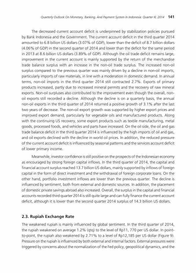
The decreased current account deficit is underpinned by stabilization policies pursued by Bank Indonesia and the Government. The current account deficit in the third quarter 2014 amounted to 6.8 billion US dollars (3.07% of GDP), lower than the deficit of 8.7 billion dollars (4.06% of GDP) in the second quarter of 2014 and lower than the deficit for the same period in 2013 at 8.6 billion US dollars (3.89% of GDP). Although the oil trade deficit remains large, improvement in the current account is mainly supported by the return of the merchandise trade balance surplus with an increase in the non-oil trade surplus. The increased non-oil surplus compared to the previous quarter was mainly driven by a decline in non-oil imports, particularly imports of raw materials, in line with a moderation in domestic demand. In annual terms, non-oil imports in the third quarter 2014 still contracted 2.7%. Exports of primary products increased, partly due to increased mineral permits and the recovery of raw mineral exports. Non-oil surpluses also contributed to the improvement even though the overall, non-oil exports still recorded a decline. Although the decline is on a quarterly basis, the annual non-oil exports in the third quarter of 2014 returned a positive growth of 3.1% after the last two years of decrease. The non-oil export growth was supported by higher export prices and improved export demand, particularly for vegetable oils and manufactured products. Along with the continuing US recovery, some export products such as textile manufacturing, metal goods, processed foods, and vehicles and parts have increased. On the oil side, the oil and gas trade balance deficit in the third quarter 2014 is influenced by the high imports of oil and gas, and oil exports declined with the decline in world oil prices. In addition, the reduced pressure of the current account deficit is influenced by seasonal patterns and the services account deficit of lower primary income.
Meanwhile, investor confidence is still positive on the prospects of the Indonesian economy as encouraged by strong foreign capital inflows. In the third quarter of 2014, the capital and financial account surplus reached 13.7 billion US dollars, mainly supported by inflows of foreign capital in the form of direct investment and the withdrawal of foreign corporate loans. On the other hand, portfolio investment inflows are lower than the previous quarter. The decline is influenced by sentiment, both from external and domestic sources. In addition, the placement of domestic private savings abroad also increased. Overall, the surplus in the capital and financial accounts recorded third quarter 2014 is still quite large and can fully finance the current account deficit, although it is lower than the second quarter 2014 surplus of 14.3 billion US dollars.
2.3. Rupiah Exchange Rate
The weakened rupiah is mainly influenced by global sentiment. In the third quarter of 2014, the rupiah weakened on average 1.2% (qtq) to the level of Rp11, 770 per US dollar. In point-to-point, the rupiah also weakened by 2.71% to a level of Rp12,185 per US dollar (Figure 9). Pressure on the rupiah is influenced by both external and internal factors. External pressures were triggered by concerns about the normalization of the Fed policy, geopolitical dynamics, and the

142 Bulletin of Monetary, Economics and Banking, Volume 17, Number 2, October 2014
2.4. Inflation
Inflation maintained its downward trend that is supported by the prospect of achieving the 2014 inflation target of 4.5 ± 1%. Inflation in the third quarter of 2014 is 4.53% (yoy), down from 6.70% (yoy) in the previous quarter. Inflation is maintained and supported by the control of the core inflation and foods volatility. Unbridled core inflation was supported by a decline in global commodity prices, moderate demand and subdued inflation expectations. Meanwhile, volatile food inflation is also relatively low, due to a sufficient food supply. By contrast, inflation in administered prices increased, mainly driven by increases in the TTL RT and LPG of 12 kg.
The downward trend in inflation in the third quarter of 2014, is supported by, among others things, a relatively low volatile food inflation rate. The volatile food inflation in the third quarter 2014 is 4.21% (yoy), lower than the second quarter of 2014 which was 6.74% (yoy) (Figure 11). The drop in inflation is mainly driven by high enough food supplies and relatively smooth distribution. The commodity price corrections of onion varieties eased inflation, as a result of a harvest supply glut that took place at a variety of production centers. Meanwhile, the price of rice in this quarter is relatively restrained, in line with the forecasts of a sufficient
global economic slowdown. The external pressures also affected the currencies of countries in the region, including Indonesia (Figure 10). The weakening rupiah was influenced by internal factors to Indonesia, such as the behavior of investors who awaited the formation of the new cabinet and the government work program. Depreciation pressure in the third quarter 2014 is reflected on some external indicators such as the VIX Index and CDS that increased. However, the volatility of the rupiah is still controlled, and lower than the Turkish lira, Brazilian real and South African rand. Looking ahead, Bank Indonesia will continue to maintain the stability of the exchange rate in accordance with fiscal fundamentals.
Figure 9.Rupiah Exchange Rate
Figure 10.Regional Exchange Rates
� � ������ � � ���� �� � ��� �� �� � ��� ���� � � ���� ���� � ������ � � �� ���� ����� �� ��� � ������
�������
��� ��� ��� �� ��� �� � � ���
������
������
������
������
������
������
������ ������
������
������������ ������
������
������
������������
������
�������������������������� ����������� �������������
������ ������ ����� ����� ����� ����� ���� �����
���
���
���
���
� �
���
��
��
���
���
������������������
�������������� ������
����
����
����
����
�����
�����
�����
�����
�����
�����
�����
�����
�����
�����
�����
�����
�����
�����
�����
����

143Quarterly Outlook On Monetary, Banking, And Payment System In Indonesia: Quarter III, 2014
supply of rice at the end of the harvest season. In addition, a weakened El Nino in the fourth quarter also contributed in controlling volatile food inflation in the third quarter of this year.
Decline in inflation in the third quarter 2014 is also supported by control of the core inflation in line with the decrease of external and domestic pressures. Core inflation in the third quarter 2014 is recorded at 4.04% (yoy), down compared to the previous quarter at 4.81% (yoy). Reduced external pressure is primarily driven by a decrease in global prices, amid pressure of a weakening rupiah at the end of the third quarter of 2014. Domestically, despite an increased seasonal demand due to the Muslim Holiday of Eid and the new school year, the pressure of demand is fundamentally slowed with declining economic activity. In addition, inflation expectations in the third quarter is still restrained.
There are indications of rising inflationary expectations related to oil price hikes. This is reflected in higher inflation expectations by retailers by the end of 2014 in line with the increasing concern of rising fuel prices (Figure 12). In addition, an indication of rising inflation expectations is also reflected in the financial sector.
Meanwhile, inflationary pressures from administered prices increased mainly driven by higher TTL RT. The impact of rising TTL Household group (R-2 and R-1) Phase I (July 1, 2014) and Phase II (1 September 2014) as well as the adjustment of rates for group R-3 (> 6600VA) encouraged high inflation as contributed by the electricity rates reaching 0.25%. In addition, the increase in seasonal demand ahead of the Muslim Holiday Eid pushes up rates of transportation groups such as inter-city transport and air transport.
Spatially, the inflation pressure in the third quarter in the various regions is relatively restrained. It is powered by low volatile food inflation with adequate food supplies amid rising
Figure 11Annual Inflation
Figure 12Retailer Price expectations
����
� � � � ���� � � � ���� � � � ���� � � � ���� � � � ���� � � � ���� � � �
������
���� ���� ���� ���� ���� ���� ����
���
��
�
�
��
��
����
����
����
��������� ��� ����������������������
����������
�����
� �� � ���� �� � ���� �� � ���� �� � ��� � �� � ��� � �� � ���� �� � ��� � �� � ��� � �� � ���� �� � �
���� ���� ���� ���� ���� ���� ���� ���� ��������
���
���
���
���
���
��� ��
��
��
�
�
��� �
�������� ������������������ �������������������������������������� �� �������������������������������������� ��

144 Bulletin of Monetary, Economics and Banking, Volume 17, Number 2, October 2014
demand for the religious festivities. However, some areas such as West Sumatra, Bengkulu, Bangka Belitung, Banten, and West Kalimantan noted high inflation, in the range of 6% (yoy), as a result of a rise in TTL and LPG 12 kg (Figure 13).
III. THE DYNAMICS OF MONETARY, BANKING, AND PAYMENT SYSTEM
3.1. Monetary
The interest rates and money supply development is still in accordance with the direction of the monetary policy adopted by Bank Indonesia. During the third quarter of 2014, interbank rates were relatively stable while bank interest rates still maintained an upward trend. An increase in interest rates occurred amid slowing economic growth in the third quarter of 2014, and its effect on the dynamics of liquidity in the economy is relatively stable even though liquidity in the interbank market tended to increase.
The Interbank Money Market in the third quarter 2014 is marked by a relatively stable the interbank O/N rate, while the average total volume of the Interbank Money Market is in relative decline. This indicates that the liquidity conditions in the overnight Interbank Money Market is relatively stable. The weighted average interbank rate in the third quarter 2014 amounted to 5.86% which is relatively the same compared to the previous quarter. Relatively stable interest rate movements of the Interbank Money Market triggered an overnight spread effect to stabilize the overnight deposit facility at 11bps, while having a similar effect on the BI rate which also stabilized at 164bps, indicating an absence of the liquidity crunch on the interbank money market. While the average total volume of Interbank Money Market showed a relative decrease from Rp12.1 trillion to Rp11.8 trillion, the average volume of the overnight
Picture 2.Distribution maps of Consumer Price Index (CPI) Inflation (%, yoy)
Inf > 6.2% 4.1% < Inf < 5.0% Inf < 4.1%5.0% < Inf < 6.2%
ACEH5.4
SUMUT4.4
RIAU5.5
KEP. BABEL5.4
DKI JAKARTA5.2 JATENG
5
SULTENG7.3
KALTIM4.6
KALBAR5.4
SULUT6.4
MALUT5.9
PAPBAR5.1
PAPUA4.7
BALI5.1 NTT
4.6
KEP. RIAU4.5
LAMPUNG4.5
BENGKULU5.8
BANTEN6.7
SULSEL4.7
SULBAR4.4
JABAR4 JATIM
4.6NTB4.7
KALTENG5.2
KALSEL5.6
GORONTALO3.7
MALUKU6
SULTRA3.3
SUMSEL3.4
JAMBI4.1
DIY4.4
SUMBAR6.3
National: 4.83% (yoy)
145Quarterly Outlook On Monetary, Banking, And Payment System In Indonesia: Quarter III, 2014
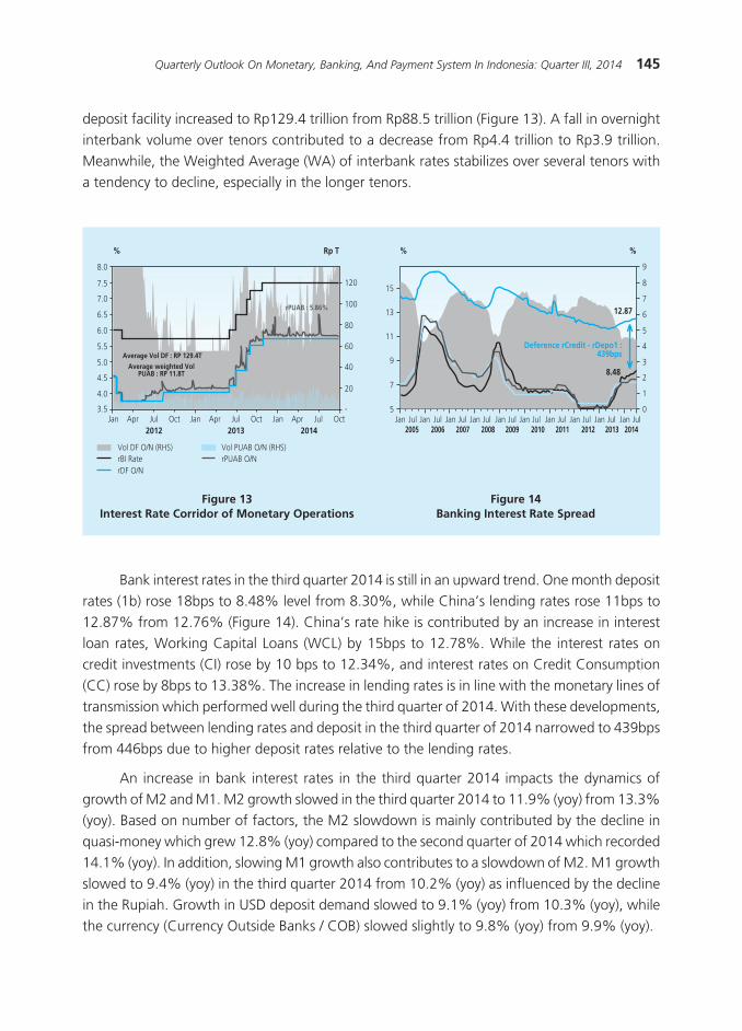
Bank interest rates in the third quarter 2014 is still in an upward trend. One month deposit rates (1b) rose 18bps to 8.48% level from 8.30%, while China’s lending rates rose 11bps to 12.87% from 12.76% (Figure 14). China’s rate hike is contributed by an increase in interest loan rates, Working Capital Loans (WCL) by 15bps to 12.78%. While the interest rates on credit investments (CI) rose by 10 bps to 12.34%, and interest rates on Credit Consumption (CC) rose by 8bps to 13.38%. The increase in lending rates is in line with the monetary lines of transmission which performed well during the third quarter of 2014. With these developments, the spread between lending rates and deposit in the third quarter of 2014 narrowed to 439bps from 446bps due to higher deposit rates relative to the lending rates.
An increase in bank interest rates in the third quarter 2014 impacts the dynamics of growth of M2 and M1. M2 growth slowed in the third quarter 2014 to 11.9% (yoy) from 13.3% (yoy). Based on number of factors, the M2 slowdown is mainly contributed by the decline in quasi-money which grew 12.8% (yoy) compared to the second quarter of 2014 which recorded 14.1% (yoy). In addition, slowing M1 growth also contributes to a slowdown of M2. M1 growth slowed to 9.4% (yoy) in the third quarter 2014 from 10.2% (yoy) as influenced by the decline in the Rupiah. Growth in USD deposit demand slowed to 9.1% (yoy) from 10.3% (yoy), while the currency (Currency Outside Banks / COB) slowed slightly to 9.8% (yoy) from 9.9% (yoy).
����������������������� ��
��� �������� ��� ������ ��� ��� ������ ��� ��� ������
���
���
���
���
���
���
���
���
���
��
�������������������������������� ��
��������� ���
�����
�
��
��
��
�
��
��
������������������������������
��� ������������� ������
��� ��� ��� ��� ��� ��� ��� ��� ��� ��� ��� ��� ��� ��� ��� ��� ��� ��� ��� ����
�
�
��
��
��
�
�
�
�
�
�
�
�
�
�
�
�
�����
����������������������� ������ �
���
���� ���� ���� ���� ���� ���� ���� ���� ��� ���
deposit facility increased to Rp129.4 trillion from Rp88.5 trillion (Figure 13). A fall in overnight interbank volume over tenors contributed to a decrease from Rp4.4 trillion to Rp3.9 trillion. Meanwhile, the Weighted Average (WA) of interbank rates stabilizes over several tenors with a tendency to decline, especially in the longer tenors.
Figure 13Interest Rate Corridor of Monetary Operations
Figure 14Banking Interest Rate Spread

146 Bulletin of Monetary, Economics and Banking, Volume 17, Number 2, October 2014
Based on the above factors, the decline of Net Foreign Assets (NFA) is a major factor for the decline in M2 amidst an increase in Net Domestic Assets (NDA). NFA growth slowed to 14.6% (yoy) from 29.2% (yoy), while the NDA increased from 8.1% (yoy) to 10.5% (yoy). The NFA decrease is influenced by a decrease in foreign exchange reserves of the central bank and increased (net) liabilities of commercial banks to non-residents (NR); whereas the increase in NDA is due to increased bills to the central government.
3.2. Banking Industry
The stability of the financial system remains solid sustained by the resilience of the banking system and the relatively subdued performance of the financial markets. The resilience of the banking industry remains strong although credit risk and market liquidity is fairly maintained, as well as strong capital backing. A relatively stable financial market performance is supported by relatively good capital market performance during the third quarter 2014 and an increase in yield of government securities in all tenors on a quarterly basis.
The pace of credit growth slowed contributed by Working Capital Loans (WCL). As of the third quarter of 2014, credit growth slowed to 13.2% (yoy) from 17.2% (yoy); yet grew 8.2% (ytd). Slowing the rate of credit is still contributed by Credit for Working Capital (CWC) that has a share of 48.0%, (whereas the share of CI and CC is 24.5% and 27.5%, respectively). Based on its use; the CWC type of credit growth and CI fell to 13.3% (yoy) and 16.4% (yoy) from 17.3% (yoy) and 22.5% (yoy), respectively compared to the second quarter of 2014. Similarly, credit growth of CC types also fell to 10.1% (yoy) from 12.7% (yoy) (Figure 15). By sector, the trade sector still has the largest share of total loans which reached 22%, and is followed by the processing industry with a share of 18%. Slowing credit expansion is contributed by
Figure 15.Loan Growth by Expenditure
Figure 16.Growth in Deposits
��� ��� ��� ��� ��� ��� ��� ��� ��� ��� ��� ��� ��� ��� ��� ��� ��� ��� ���
������������������
���� �������� ���� ����
�����
��
�
��
�
�
��
��
���
��
�������������
�������
��
��
�
�
�
�
���� ��� ��� ��� ��� ��� ��� ��� ��� ��� ��� ��� ��� ��� ��� ��� ��� ��� ���
������
���� ���� ���� ���� ����
�
�
��
��
��
��
�� �� ���������������������������
��������������������������������� ����
��
�
�
��
��
��
147Quarterly Outlook On Monetary, Banking, And Payment System In Indonesia: Quarter III, 2014
manufacturing and trade. The manufacturing sector growth slowed to 16.1% (yoy) from 24.9% (yoy), while the trade sector credit growth also slowed to 13.9% (yoy) from 18.3% (yoy).
Deposit growth slowed slightly, triggered by a decrease in the Current Account Savings Account (CASA), which consists of current and savings accounts. In the third quarter of 2014, the demand for deposits and savings growth slowed to 7.0% (yoy) and 7.1% (yoy) from 10.2% (yoy) and 9.5% (yoy), respectively. Actual deposit growth increased to 21.4% (yoy) from 18.5% (yoy). Thus, the slowdown in deposit growth is contributed by the decline in the CASA, which fell to 53.1% in the third quarter 2014 from 54.2% in the previous quarter (Figure 17). Although lower than the second quarter of 2014, growth in deposits in September 2014 increased compared to the previous month and stood at 13.32% (yoy). This is in line with the government’s financial operations which were expansionary. Further, the bank liquidity in the third quarter of 2014 is maintained.
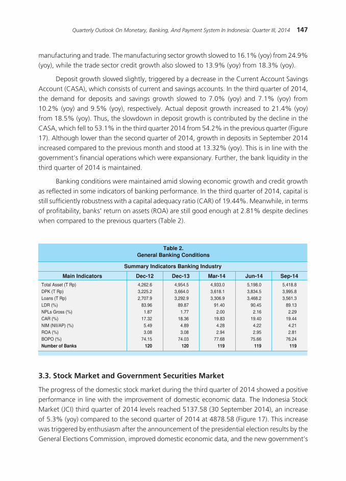
Banking conditions were maintained amid slowing economic growth and credit growth as reflected in some indicators of banking performance. In the third quarter of 2014, capital is still sufficiently robustness with a capital adequacy ratio (CAR) of 19.44%. Meanwhile, in terms of profitability, banks’ return on assets (ROA) are still good enough at 2.81% despite declines when compared to the previous quarters (Table 2).
3.3. Stock Market and Government Securities Market
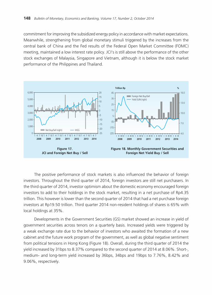
The progress of the domestic stock market during the third quarter of 2014 showed a positive performance in line with the improvement of domestic economic data. The Indonesia Stock Market (JCI) third quarter of 2014 levels reached 5137.58 (30 September 2014), an increase of 5.3% (yoy) compared to the second quarter of 2014 at 4878.58 (Figure 17). This increase was triggered by enthusiasm after the announcement of the presidential election results by the General Elections Commission, improved domestic economic data, and the new government’s
Table 2.General Banking Conditions
Summary Indicators Banking Industry
Main Indicators Dec-12 Dec-13 Mar-14 Jun-14 Sep-14
Total Asset (T Rp) 4,262.6 4,954.5 4,933.0 5,198.0 5,418.8DPK (T Rp) 3,225.2 3,664.0 3,618.1 3,834.5 3,995.8Loans (T Rp) 2,707.9 3,292.9 3,306.9 3,468.2 3,561.3LDR (%) 83.96 89.87 91.40 90.45 89.13NPLs Gross (%) 1.87 1.77 2.00 2.16 2.29CAR (%) 17.32 18.36 19.83 19.40 19.44NIM (NII/AP) (%) 5.49 4.89 4.28 4.22 4.21ROA (%) 3.08 3.08 2.94 2.95 2.81BOPO (%) 74.15 74.03 77.68 75.66 76.24Number of Banks 120 120 119 119 119
148 Bulletin of Monetary, Economics and Banking, Volume 17, Number 2, October 2014
The positive performance of stock markets is also influenced the behavior of foreign investors. Throughout the third quarter of 2014, foreign investors are still net purchasers. In the third quarter of 2014, investor optimism about the domestic economy encouraged foreign investors to add to their holdings in the stock market, resulting in a net purchase of Rp4.35 trillion. This however is lower than the second quarter of 2014 that had a net purchase foreign investors at Rp19.50 trillion. Third quarter 2014 non-resident holdings of shares is 65% with local holdings at 35%.
Developments in the Government Securities (GS) market showed an increase in yield of government securities across tenors on a quarterly basis. Increased yields were triggered by a weak exchange rate due to the behavior of investors who awaited the formation of a new cabinet and the future work program of the government, as well as global negative sentiment from political tensions in Hong Kong (Figure 18). Overall, during the third quarter of 2014 the yield increased by 31bps to 8.37% compared to the second quarter of 2014 at 8.06%. Short-, medium- and long-term yield increased by 36bps, 34bps and 19bps to 7.76%, 8.42% and 9.06%, respectively.
� � � �� � � � �� � � � �� � � � �� � � � �� � � � �� � � ����� ���� ���� ���� ���� ���� ����
���
�
�
��
��
��
��
���
���
���
�
�����
�����
�����
�����
�����
�����
�������� ������������
� �� ��� �� � �� ��� �� � �� ��� �� � �� ��� �� � �� ��� �� � �� ��� �� � �� ������� ���� �������� ���� ���� ����
����
����
���
�
��
��
��
��
���
���
����
����
��������� ������������
����������� �
������������ ��
commitment for improving the subsidized energy policy in accordance with market expectations. Meanwhile, strengthening from global monetary stimuli triggered by the increases from the central bank of China and the Fed results of the Federal Open Market Committee (FOMC) meeting, maintained a low interest rate policy. JCI’s is still above the performance of the other stock exchanges of Malaysia, Singapore and Vietnam, although it is below the stock market performance of the Philippines and Thailand.
Figure 17.JCI and Foreign Net Buy / Sell
Figure 18. Monthly Government Securities and Foreign Net Yield Buy / Sell

149Quarterly Outlook On Monetary, Banking, And Payment System In Indonesia: Quarter III, 2014
Weakening GS prices followed an increase in GS yield utilized by non-residents who continued to add to their holdings in the government securities market. During the third quarter of 2014, the net purchase of foreign investors was Rp43.79 trillion, higher than the second quarter of 2014 at Rp42.68 trillion. During the same period, ownership of government securities by banks, foreign insurance and pension funds also increased, so that the proportion of government securities holdings by BI decreased. Foreign investors were buyers of government securities throughout the tenor, so that the amount of foreign ownership in government securities in the third quarter of 2014 increased to 36.17% compared to 34.51% of the previous quarter.
3.4. Payment System Developments
Payment system developments in the cash group is generally in line with the development of the domestic economy, especially the household consumption sector. The daily average currency in circulation in the third quarter 2014 amounted to Rp491.3 trillion and grew 12.6% (yoy), down from the previous growth quarter of 13.9% (yoy), and likewise down for the same quarter of the previous year at 11.1% (yoy). The currency in circulation is in line with the slowing growth in household consumption and GDP of quarterly reports.
In the middle of the currency in circulation growth trend, Bank Indonesia continued to improve the feasibility of the money supply. During the third quarter of 2014, some 1.3 billion pieces / chips of Money-Not-Fit for-Circulation (MNFC) worth Rp29.7 trillion was destroyed and replaced with money fit for circulation. Total destruction of MNFC was higher than the second quarter of 2014 totaling 1 billion pieces / chips or Rp22.6 trillion worth of currency. The increased MNFC destruction was due to the increased amount of money in conditions not fit for circulation that were deposited by banks to Bank Indonesia.
The fixed payment transactions system ran smoothly during the third quarter of 2014. In the third quarter 2014 the non-cash payment system transactions increased both in terms of value and volume of transactions. The increased value of transactions stood at Rp8, 742.8 trillion (QtQ rise by 26.97%), and an increase in the volume of transactions stood at 36.12 million transactions (QtQ rise by 3.16%) when compared to the previous quarter (Table 3). In the reporting period, the increase in the value of the transactions occurred in all groups, especially monetary transactions. On the other hand, the increase in the volume of transactions caused by increasing public transactions through non-cash instruments was in line with the celebrations of the Muslim Eid Festivities and the Presidential general election of 2014.

150 Bulletin of Monetary, Economics and Banking, Volume 17, Number 2, October 2014
In harmony with the increase in the value and volume of the non-cash payment system transactions in the third quarter of 2014, payment transactions settled through the Bank Indonesia Real Time Gross Settlement (BI-RTGS) also increased both in terms of value and volume. The BI-RTGS is the fund settlement system. The Bank Indonesia-Scripless Securities Settlement System (BI-SSSS), as well as the Funds Transfer and Scheduled Clearing by Bank Indonesia (SKNBI) reached 100% in the third quarter of 2014. The value of transactions of settled payments through the BI-RTGS increased by Rp5, 716.17 trillion (QtQ rose by 23.67%) to reach Rp Rp29, 866.56 trillion compared to the previous quarter was at Rp24, 150.39 trillion. The volume of payment transactions settled through the BI-RTGS increased by 48.60 thousand (QtQ rose by 1.09%) to reach 4.52 million transactions, compared with the previous quarter at 4.47 million transactions.
IV. ECONOMIC OUTLOOK
Bank Indonesia expects the economy will still experience an adjustment while macroeconomic stability is maintained. Economic growth in 2014 is estimated to be at the lower limit of 5.1 to 5.5% projection. It is affected by the growth of the world GDP that is not as strong as earlier forecasted and budget savings for the State Budget Year 2014. The projected growth in the world economy is expected to be weak resulting from export performance that is not as strong as previously expected, while the government’s austerity budget pushes a slowdown in government consumption. By 2015, economic growth is expected to bounce back and be in the range of 5.4 to 5.8%. Improvement is in line with global economic forecasts of conditions that would be better than a year earlier. This would contribute to export growth which is also forecasted to increase.
In line with the moderation of economic growth, inflation in 2014 is estimated to be lower than inflation in 2013 and will be heading towards the 2015 inflation target of 4 + 1%. In quarter IV-2014, inflation is expected to increase again in line with the assumption
Table 3.Non-Cash Payment System Developments
Non-Cash PaymentSystem Transaction
2013
Q1 Q2 Q3 Q4 Q1 Q2 Q3
2014
BI-RTGS 18,778.31 21,410.40 26,369.50 24,403.80 23,817.80 24,150.40 29,866.56 BI-SSSS 4,939.05 5,299.70 8,259.90 8,233.40 7,173.60 6,396.90 9,366.77Clearance 547.87 605.70 680.80 708.00 667.80 710.70 716.36APMK 901.67 989.60 1,039.40 1,073.90 1,082.20 1,158.52 1,208.91Credit Card 51.09 55.23 57.08 59.62 59.78 63.65 64.41ATM Card & ATM/Debit 850.58 934.38 982.36 1,014.28 1,022.42 1,094.87 1,144.50Electronic Money 0.59 0.68 0.90 0.74 0.73 0.83 0.86Total 25,167.48 28,306.07 36,350.55 34,419.79 33,860.26 32,417.39 41,159.47

151Quarterly Outlook On Monetary, Banking, And Payment System In Indonesia: Quarter III, 2014
that the exchange rate would further depreciate and air freight rates would increase. With such developments, inflation in 2014 is estimated upwards. Meanwhile, inflation for 2015 is expected to rise related to the adjustment of some administered prices, such as the upper limit air freight rates and the price of LPG (March and August 2015), as well as the projection of the high pressures on volatile foods and further exchange rate depreciation. However, inflation in 2015 is estimated to be in the target range of 4.0 ± 1%
Bank Indonesia will keep a close watch some of the risks shadowing the economic adjustment process going forward. Globally, among other risks associated with the normalization of the Fed’s policy plans, is the economic vulnerability of emerging markets and economic weakness in a number of countries. On the domestic front, the risk that requires attention is the potential for inflationary pressures due to adjustments in administered prices such as subsidized fuel prices and electricity tariffs. In addition to inflation, domestic risks also arise from the potential reversal of capital flows (capital reversal) with the normalization of the Fed’s policy and high foreign debt position.

152 Bulletin of Monetary, Economics and Banking, Volume 17, Number 2, October 2014
This page intentionally left blank
153The Determining Factors Of Currency Redenomination Success: Experimental And Historical Aproach
THE DETERMINING FACTORS OF CURRENCY REDENOMINATION SUCCESS:
EXPERIMENTAL AND HISTORICAL APROACH
Andika Pambudi1
Bambang Juanda2
D.S. Priyarsono2
Redenomination is a simplification of nominal value of currency by reducing digit (zero number)
without reducing the real value of the currency. The main objective of this research was to examine
whether the economic conditions at the time of redenomination may affect the success of currency
redenomination. The methods used were regression analysis on historical data of 30 countries which
are involved in redenominating their currencies, economic experiments with t-test, and survey of people’
perspective.Based on regression analysis, inflation will decrease and economic growth will rise higher
after redenomination, if previously a country have experienced high economic growth as well. Based on
experimental research, when inflation was high, redenomination could increase the selling price. Otherwise,
when inflation was low, redenomination could decrease the selling price. Changes in selling price after
redenomination was not affected significantly by differences in economic growth conditions. In different
economic conditions, redenomination policy did not significantly affect the changes number of transactions
and total value of transactions in the market. From the survey results, public did not believe government
can control inflation after redenomination. Redenomination also will not affect consumption pattern.
Abstract
Keywords: Redenomination, Inflation, Economic Growth, Experiment
JEL Classification: C91, E31, E42, E58,
1 Peneliti di Center for Public Policy Transformation (www.transformasi.org).2 Departemen Ilmu Ekonomi, Fakultas Ekonomi dan Manajemen IPB – Penulis Korespondensi ([email protected]).
154 Bulletin of Monetary, Economics and Banking, Volume 17, Number 2, October 2014
I. INTRODUCTION
Redenomination is a simplification of nominal value of a currency by reducing digits (zero number) without reducing the real value of the currency. Bank Indonesia (BI) has planned the redenomination of Rupiah by reducing three zero digits of the currency value, goods prices as well as wages. Too big nominal value of a currency reflects that in the past, a country had encountered high inflations or it had experienced a pretty bad economic fundamental condition (Kesumajaya, 2011). Moreover, if a country constantly encounters a high inflation every year, the value of the currency towards the goods will be lower (Amir, 2011). 55 countries have redenominated, some of them result in success and some result in failure. One of the indicators of the redenomination application success is the inflation rate after the redenomination being applied. It will be considered a failure if a high inflation or a hyperinflation happens after the implementation.
Nowadays, Indonesia, that plans to perform redenomination, has encountered some turmoil and instabilities in its both currency value and inflation rate. Before its independence, in 1944 the value of Rupiah was almost as valuable as USD; Rp 1,88 per USD. Then on March 7th 1946 the value crash of Rupiah happened for the first time as much as 30 percent, so it was Rp 2,65 per USD. In 1950 the government performed sanering of Rp 5 and above so the value became only half of the previous value. The government then performed the second sanering on 25th August 1959 by cutting the value of Rupiah.
The high rate of inflation results in the weakening of currency value. This can be seen that in 1960s, Indonesia encountered an extremely high hyperinflation that hit its peak in 1966 as much as 1136 percent. Subsequently, in 1971 the value of Rupiah was depreciated and it reached the value of Rp 415 per USD (World Bank, 2012). After 68 years of independence, the value of Rupiah now is about Rp 9.700 per USD. That more depreciated value becomes one of the government’s reasons to have determination to boost Rupiah’s prestige. This moment is considered right because Indonesia’s current inflation rate is relatively stable in the last few years. Even, it can be declared that the inflation is creeping (creeping inflation) in type or occurs in around one digit every year. This constant inflation reflects price stability for some goods that form consumers’ price level.
The government aims at increasing Rupiah’s credibility is a positive effect of redenomination, yet its implementation also has negative effects. One of them is the people’s misperception that they think it is a sanering. Sanering is a policy of omitting zeros in a currency, yet this cutting is not done to the goods price so the people’s purchasing power decreases. This people’s misconception of redenomination may cause a state of panic resulting in economic situation turmoil. In addition, redenomination will increase companies and banking operational expenses because they have to replace their information and technology system. They certainly need some time to implement new accounting technology to adjust to nominal simplification. Bank Indonesia will also spend high expense to issue new redenominated money as well as public

155The Determining Factors Of Currency Redenomination Success: Experimental And Historical Aproach
dissemination. Redenomination will also cause other social effects in terms of public distrust to Rupiah (Kesumajaya, 2011).
According to Wibowo (2013), an effect that will come into view because of this currency nominal change is the emergence of psychological bias so called money illusion. Most people will assume that goods price is cheaper because of the omission of zeros from the previous currency. For instance, there is an escalation of goods price as much as of Rp 7.000, consumers will find this very hard. However, after redenomination the escalation is only Rp 7 and they will find it trouble-free whereas they have exactly the same value. Consumers pay less attention to the re- scaling process of the old Rupiah nominal value to the new one. Money Illusion will affect the consumers more when they review the real value of goods they have bought because of the simultaneous nominal change. Redenomination drives into bigger consumption behavior. New prices are perceived cheaper because of money illusion and consumers’ willingness to pay increases. By seeing this people’s behavior, producers will escalate the price up to consumers’ tolerated limit.
Pros and cons of redenomination policy scheme reflect a public speculation about unpredictability of consequence that might happen if redenomination of Rupiah is implemented at the moment. Research on probable effects needs to be scientifically investigated through experimental method. According to Juanda (2010) the data of experiment results will be more easily interpreted in the effort of concluding causal relationship compared to data of survey result or secondary data. This investigation is aimed at noticing contributing factors to the success of the currency redenomination. The factors are economic condition when redenomination policy is implemented. The condition covers among others inflation rate. The success of redenomination can be seen through the change of inflation rate and the economic growth after redenomination being implemented.
The scope of this study is divided into three sections. First, it gives identification of contributing factors to the success of redenomination policy in a country through a study to secondary data that come from some historical information of countries that have redenominated. Second, it analyzes the impacts of Rupiah redenomination policy on the behaviors of economic subjects (pelaku ekonomi). The behaviors effects of the subjects will be further investigated to see the economic performance (kinerja perekonomian). Third, it records people’s perspective as producers and consumers on the currency redenomination policy. In the effort of investigating the second section of this study, the data used will be gathered through experimental method. The economic performance being investigated, like inflation rate and economic growth will be viewed based on the change of the number of transaction and the average prices after redenomination generated from the responses of experiment simulation. The term redenomination in this paper refers to the policy of three zeros reduction in the value of Rupiah, price unit, wage unit (unit harga, unit upah) and everything valued by the currency.

156 Bulletin of Monetary, Economics and Banking, Volume 17, Number 2, October 2014
II. THEORETCAL REVIEW
2.1. The Linkage of Redenomination and Economic Performance
There are relatively not many studies investigating the role of redenomination in economic performance. Yet, there are some opinions stating that a country’s decision to redenominate is strictly influenced by the prior economic condition. Additionally, the change of economic indicators in a country can also be influenced by the implementation of currency redenomination policy.
Suhendra and Handayani (2012) investigated the connection between redenomination policy and the inflation rate, exchange rate, economic growth and export value (nilai ekspor). The data on the economic indicators of 27 countries redenominated showed that inflation and economic growth were two variables significantly influenced by currency redenomination. Meanwhile, the high inflation rate was the most dominant driving factor for a country to decide to redenominate its money value. This finding is in line with what Mosley (2005) says that the current and the past inflation are the most important predictors whether or not to redenominate.
Iona (2005) investigated long-term advantages of redenomination, reasons of redenomination implementation timing, their influence to the price. The result of the study revealed that the long- term impacts of redenomination were: 1) public trust establishment to domestic currency; 2) the increase of saving in domestic currency; and 3) the money saved out of national monetary system will flow to market. Redenomination will be successfully implemented if it meets the two requirements as follow: 1) low inflation rate with decreasing tendency; and 2) the success of economic reformation and reconstruction program, like the high growth of real GDP (Gross Domestic Product). If those two requirements are met, redenomination will be useful. Iona (2005) also says that indicators that have to be monitored to assess the impacts of redenomination are Consumer Price Index, purchasing power, exchange rate, 1- month deposit average ( rata-rata deposito 1-bulan), Consumer Trust Index, Business Trust Index. (Indeks Kepercayaan Konsumen, dan Indeks Kepercayaan Bisnis).
2.2. The Relation between Redenomination and Economic Subjects’ Behaviors
Some impacts that might occur in the implementation of redenomination are the emergence of psychological bias called money illusion (Wibowo, 2013). This illusion can come into view because of the nominal change of goods price resulted from redenomination. Most people will perceive cheaper goods price due to the value omission of zero from the previous currency. Hobijn et al (2006) point out that money illusion has occurred in some European country changing their currency into Euro. Euro whose fewer nominals (nominal yang lebih sedikit) compared to the prior currency is perceived cheaper by the people. Hobijn et al (2006)

157The Determining Factors Of Currency Redenomination Success: Experimental And Historical Aproach
thinks that the escalation of the price after redenomination can be explained by the general model of menu cost price, by inputting companies’ decision when they adopt new currency.
Furthermore, consumers will re-evaluate their financial strategy management to adapt to new currency especially when the new and the old currency are used in concert, waiting for the old to disappear. Marques and Dehaene (2004) state that there are two major processes that can take place when a country adapt a new currency : rescaling (changing all prices in old currency into the new money values all at once) or re-learning ( remembering new price of the consumers’ good one at a time). The first process is predicted to experience effortless adjustment to the new currency; meanwhile the latter will encounter more complex and longer adjustment.
In the meantime, Money/Euro Illusion shows that the price perception in new denomination is smaller and lower currency than when it is stated in the previous currency if it has higher nominal (Gamble et al. 2002). This demonstrates that individuals adjust themselves to the new currency with its smaller nominal value, at least, they encounter difficulty in understanding the real value of goods and services. Money illusion’s effect can also happen to cheap goods or when the escalation of the price is only few cents. If the availability of cents (coins) is not fulfilled by the government, consumers will tend to allow the escalation of the price without demanding change from the seller. This phenomenon is called trivialization.
Trivialization case can be observed in Ghana whose inflation rate increases as much as 5% per year after redenomination. One of the factors causing the redenomination failure is that 70% of money circulating in Ghana is out of banking system. Ghana’s cash transactions are more dominant than its banking transaction. To make things worse, the government hasn’t been able to change the new currency into the old currency after two years of redenomination. Mehdi and Reza (2012) also state that the reduction of the currency nominal value will invite psychological and social impacts. When a currency has a low nominal value, then the people will think that the currency has a strong value.
Lianto and Suryaputra (2012) did a research to identify the impacts of redenomination implementation in Indonesia based on Indonesian’s perspective. The data gathered through surveying 100 people who have knowledge on redenomination and the data were then analyzed by employing Structural Equation Modelling. It could be seen that the most influential impact of redenomination was that it could increase the credibility of Indonesia in front of other countries. The other finding was that the Indonesian considered redenomination to be beneficial for them. If it was implemented successfully, Rupiah would be stronger and it would boost the people’s trust to their currency.

158 Bulletin of Monetary, Economics and Banking, Volume 17, Number 2, October 2014
2.3. The Experiment in the Study of Economic Policy
Economic experiment can be used to study an economic policy as well as to review an economic theory. One of the illustrations is what Juanda et al (2011) did in studying and comparing systemic impacts resulted from the policy of Century Bank rescue effort and its closure policy issued by the government. The result of the study showed that Century Bank closure resulted in a relatively very low impact. A sufficiently huge systemic impact would emerge if the closure in that critical time was done to an immense bank. In a normal situation (in the absence of turmoil), the closure of a small problematic bank like Century will not cause systemic impacts. Bank pressure and failure potential were extremely low since the economic stability was maintained. Thus, there was no decrease in the trust of the customers to banking.
Another research investigating a policy through experimental method is a study of tax compliance rate in the self- assessment tax collection system implemented in Indonesia (Juanda, 2010). The study looked into the influence of assessment chance impacts, fine, and educational level to the compliance of taxpayers in reporting Letter of Notification (Surat Pemberitahuan (SPT)), by controlling other factors, they were arranged to be the same (ceteris paribus). Factors that influenced taxpayers’ compliance rate were difficult to do through survey design because of environmental influences or objects of the study. Study result confirmed that the higher the tax assessment change and the bigger the fine would positively influence the taxpayers’ compliance in doing tax liabilities. Additionally, Juanda (2010) observed the tax compliance rate of “experiment subject” undergraduate students was higher compared to graduate students whose relatively higher knowledge. Moreover, the higher the taxpayers’ income, the lower their compliance was.
III. METHODOLOGY
3.1. Kinds and Data sources
The data used in this study were both primary and secondary data. Primary data were gathered through experiment. The primary data gathered were the responses of the subjects (simulation subjects) as the economic subjects in the experiment could be observed from the decisions they took. Additionally, the primary data were also collected through a survey to 168 respondents consisted of 86 lecturers of IPB, 27 IPB students, and 55 of the general public to see their perspectives on redenomination policy impacts on the national economy. This survey was intended to gain judgements, opinions and perspectives about the redenomination policy that would be implemented by the government.

159The Determining Factors Of Currency Redenomination Success: Experimental And Historical Aproach
Table 1.Countries that Have Redenominated Their Currency
No
1 Finland 1963 2 2 Iceland 1981 2 3 Israel 1985 3 4 Bolivia 1987 6 5 Uganda 1987 2 6 Nicaragua 1988 3 7 Peru 1991 6 8 Argentina 1992 4 9 The Sudan 1992 1 10 Latvia 1993 2 11 Letonia 1993 200 Rublu = 1 Lats 12 Macedonia 1993 2 13 Mexico 1993 3 14 Moldova 1993 3 15 Uruguay 1993 3 16 Brazil 1994 2,750 Cruzeiros Reais = 1 Real 17 Croatia 1994 3 18 Georgia 1995 6 19 Poland 1995 4 20 Ukraine 1996 5 21 Russia 1998 3 22 Angola 1999 6 23 Bulgaria 1999 3 24 Belarus 2000 3 25 Romania 2005 4 26 Turkey 2005 6 27 Azerbaijan 2006 1 28 Mozambique 2006 3 29 Ghana 2007 4 30 Venezuela 2008 3
Source: Iona (2005)
Countries Redenomination time Omitted Zeroes
In the interim, the secondary data employed in this study were the historical data of 30 countries that had redenominated their currency since 1963 until 2008 and they are presented in Table 1. The historical data consisted of some macro-economy indicators in the year, in which redenomination was implemented in a certain country and a year after that. The variables used were inflation rate, economic growth, exchange rate, the growth of money in circulation and the government form. The secondary data were collected from the publications of World Bank, International Monetary Fund, and Center for Systemic Peace. Information about the resources of the employed variables in the analytical model is presented as follow.

160 Bulletin of Monetary, Economics and Banking, Volume 17, Number 2, October 2014
3.2. Multiple Regression Model
The estimation method that was used to study influential factors to the implementation of redenomination employed multiple regressions. Exogenous variables or independent variables in this study were inflation rate, economic growth, exchange rate, the growth of money in circulation and the government form. Meanwhile, observed variables (endogenous) or dependent variable was the success or failure of the redenomination implementation that was measured through inflation rate and economic growth a year after redenomination was implemented in each country.
In this study, regression process was done by regressing independent variables in form of economic performance of a country that was influential to the success or the failure of redenomination (dependent variables). Dependent variable (Y) or influenced variable was economic performance indicators that reflected the success of redenomination implementation. Thus, this variable used economic performance accomplishment a year after the policy. In the meantime, independent variables (X) or the influential variables was a country economic performance when redenomination was implemented for the first time. This model had never been applied before in its relation to currency redenomination. And, the linier regression model in this study was as follow.
(1)
Inflation rate (%) World Bank, 2012, World Development Indicators 2012. (http://data.worldbank.org/indicator/FP.CPI.TOTL.ZG)
Economic growth (%) World Bank, 2012, World Development Indicators 2012. (http://data.worldbank.org/indicator/NY.GDP.MKTP.KD.ZG)
Exchange rate to USD ($ US) World Bank, 2012, World Development Indicators 2012. (http://data.worldbank.org/indicator/PA.NUS.FCRF)
The growth of money in World Bank, 2012, World Development Indicators 2012. circulation (%) (http://data.worldbank.org/indicator/FM.LBL.BMNY.ZG)
The government form index The Center for Systemic Peace, 2012, Polity IV Project (http://www.systemicpeace.org/polity/polity4.htm)
Indicator Source

161The Determining Factors Of Currency Redenomination Success: Experimental And Historical Aproach
where:
β0 = Intercept
β1,... β9 = Parameter
Yafter redenoi = Success indicator of currency redenomination for country number-i:
a) Low inflation a year after redenomination (percent)
b) Economic growth a year after redenomination (percent)
Dlowinflation- i = Dummy condition low inflation rate in the year of redenomination implantation for country number-i, with the value of:
1 = low inflation (< 10%) and 0 = high inflation (≥10%)
GROi = Economic growth in the year of redenomination implementation for country number-i (percent)
LnEXRi = Natural Logarithm of currency exchange rate to dollar in the year in which redenomination is implemented for country number -i ($ US/ Domestic Currency)
MONi = The growth of money in circulation in the year of redenomination implementation for country number -i (percent)
POLi = The government form index in the year of redenomination implementation for country number -i (percent), with the value of
min = -10 (very autocratic); max = 10 (very democratic)
Some assumptions underlying the model are: (i) dependent variable is a non- stochastic (fixed) variable, it means that it has been specified or not a random variable; (ii) there is no perfect linier relationship between independent variables or there is no collinear problem; (iii) a residual component εi has expectation value equal zero or E(εi) = 0; (iv) constant variance for all observations or var(εi) = σ2; (v) there is no relation or correlation between residue εi or cov(εi, εj) = 0 for i ≠ j; and, (vi) residual component is normally distributed.
Hypothesis Testing of Regression Parameter
Subsequently, to partially see the influence of the independent variables, t-test was used. This test will be useful if variance analysis test shows, at least, one independent variable influence the dependent one. This t-test employment is advantageous to show which independent variable is the most influential to the dependent variable. The partial hypothesis could be formulated as follow.

162 Bulletin of Monetary, Economics and Banking, Volume 17, Number 2, October 2014
H0 : βi= 0
H1 : βi ≠ 0; (i=1,2,3,4)
While the statistical test could be formulated as follow.
(2)
Null hypothesis is accepted if the absolute value of t is bigger than the t-table or if the p-value is smaller than level level of significance (α) as big as 10 percent, then null hypothesis is rejected or in other words H1 is accepted. It means that independent variable i is influential to dependent variable if other factors are constant (cateris paribus). Value-p is a probability (risk) of error in drawing conclusion of H1.
3.3. Experiment Simulation Design
This experiment was a simulation of economic activity to see the influence or response of currency redenomination towards producers and consumers behavioral change. The response to economic behavior change could be seen from the percentage of selling price change after redenomination as a proxy of inflation rate, the percentage of number of transaction change after redenomination as well as the percentage of transaction value change after redenomination as a proxy of the economic growth rate.
The economic experiment in this study involved 48 undergraduate students of IPB Economy and Management Faculty as experimental subjects. They were divided into four treatment combinations, so each combination consisted of 10 or 14 students. In the group of high growth economy treatment, 5 people acted as sellers and 5 others as buyers. In the other group of high-growth economy treatment, both buyers and sellers were seven people. The choice of respondents acting as buyers or sellers was done through drawing system. Factors that would be observed to see their influences were:
1. Economic growth, consisted of two levels: 1) high- economy growth (seven sellers and seven buyers); and 2) low-growth economy (five sellers and five buyers).
2. Inflation rate consisted of two levels: 1) high inflation (the unit cost of seller is big); and 2) low inflation (the unit cost of seller was small).
Each seller of each group was given a unit cost to goods they were going to sell. At the same time, each buyer was also given a unit value for goods they were going to buy. The sellers acted as two producers by offering two kinds of product and so did the subject. Each one of experiment subject acting as buyers also became two consumers, thus they had two different unit values. The first unit value and the second couldn’t be accumulated because they
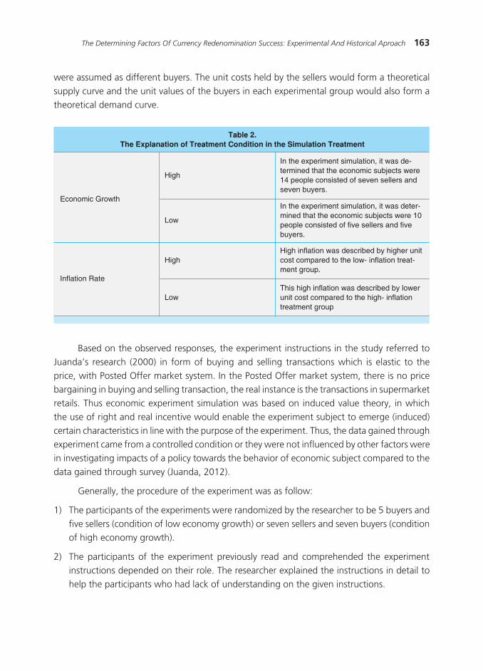
163The Determining Factors Of Currency Redenomination Success: Experimental And Historical Aproach
were assumed as different buyers. The unit costs held by the sellers would form a theoretical supply curve and the unit values of the buyers in each experimental group would also form a theoretical demand curve.
Based on the observed responses, the experiment instructions in the study referred to Juanda’s research (2000) in form of buying and selling transactions which is elastic to the price, with Posted Offer market system. In the Posted Offer market system, there is no price bargaining in buying and selling transaction, the real instance is the transactions in supermarket retails. Thus economic experiment simulation was based on induced value theory, in which the use of right and real incentive would enable the experiment subject to emerge (induced) certain characteristics in line with the purpose of the experiment. Thus, the data gained through experiment came from a controlled condition or they were not influenced by other factors were in investigating impacts of a policy towards the behavior of economic subject compared to the data gained through survey (Juanda, 2012).
Generally, the procedure of the experiment was as follow:
1) The participants of the experiments were randomized by the researcher to be 5 buyers and five sellers (condition of low economy growth) or seven sellers and seven buyers (condition of high economy growth).
2) The participants of the experiment previously read and comprehended the experiment instructions depended on their role. The researcher explained the instructions in detail to help the participants who had lack of understanding on the given instructions.
Table 2.The Explanation of Treatment Condition in the Simulation Treatment
Economic Growth
Inflation Rate
High
Low
High
Low
In the experiment simulation, it was de-termined that the economic subjects were 14 people consisted of seven sellers and seven buyers.
In the experiment simulation, it was deter-mined that the economic subjects were 10 people consisted of five sellers and five buyers.
High inflation was described by higher unit cost compared to the low- inflation treat-ment group.
This high inflation was described by lower unit cost compared to the high- inflation treatment group

164 Bulletin of Monetary, Economics and Banking, Volume 17, Number 2, October 2014
3) The participants were given a decision sheet based on their own role. Every participant had to jot down every transaction they did during the experiment period on the decision sheet for every repetition.
4) The sellers and the buyers got their own unit value and cost value.
5) In the first repetition, the buyers would be separated with the sellers in which the buyers would leave the room. The sellers had to determine the selling price above the unit cost for the condition before redenomination, then the sellers directly decided the selling price for the condition after redenomination in which the selling price could stay the same, more than or less than the price before redenomination.
6) The order of the buyers was drown then they entered the seller room to buy something one by one. The buyers had to buy goods with the price below their unit value.
7) Every seller and buyer had to note the result of their transaction on the available decision sheet.
8) Every experiment participant had the same procedure for every repetition, but the initial condition was determined randomly by the researcher in the initial repetition.
9) At the end of the experiment (repetition), the participants submitted their decision sheet to the researcher.
10) The revenue gained by each participant was then calculated based on the transaction attached on the participants’ decision sheet.
3.4. Uji Beda ( Mean Difference Testing for two independent populations)
The primary data resulted from economy experiment design would be analyzed by using Mean Difference Testing for two independent populations where they were two treatment combination groups or different economic conditions. Two groups are considered independent to each other if the choice of first example units doesn’t depend on how the second example units are chosen and vice versa (Matjik and Sumertajaya, 2002). Before comparing the two populations, firstly, we had to pay attention to the homogeneity condition of the populations that would be compared.
According to Matjik and Sumertajaya (2002), data homogeneity of the two populations can be divided into two, homogenous or σ1
2 = σ22 = σ2 and heterogeneous or σ1
2 ≠ σ22 ≠ σ2 . The
two aforementioned conditions will actually determine the accuracy of the gained conclusion. Thus, the right decision method is needed for every condition. The hypotheses for the two conditions were the same as follow.
1. H0 : μ1 – μ2 ≥ 0
H1 : μ1 – μ2< 0; or

165The Determining Factors Of Currency Redenomination Success: Experimental And Historical Aproach
2. H0 : μ1 – μ2 ≤ 0
H1 : μ1 – μ2> 0
Although the hypotheses for the two homogenous conditions were the same, the standard error that was used in the calculation of statistik uji (statistic test) was different. This could be shown as follow:
If it is proven to have the same variance (σ12 = σ2
2 = σ2) then the statistical test is as follow.
(3)
(4)
(5)
With the degree of freedom n1 + n2 – 2. In this case, Sg was stated as combined of the example 1 variance and the example 2 variance. Meanwhile if the variances were different (σ1
2 ≠ σ2
2 ≠ σ2) , the statistical test was as follow.
where,
= mean of the units in the first example
= mean of the units in the first example
μ1 = mean of the first population
μ2 = mean of the second population
s21 = variance of the first example
s22 = variance of the first example
n1 = the number of the first example units
n2 = the number of the second example unit
To determine the critical region to reject null hypotheses, it extremely depends on three things namely the form of research hypothesis (H1), statistical test that is used and the size of

166 Bulletin of Monetary, Economics and Banking, Volume 17, Number 2, October 2014
level of significance (α). The direction of null hypotheses rejection is in the same direction with the research hypothesis, as follow.
If H1 : μ1 – μ2< 0 then the critical region Tcalc< - Tα, db
If H1 : μ1 – μ2> 0 then the critical region Tcalc> Tα, db
Besides employing Tcalc , the rule in deciding whether it is significant or not in the conditions being compared is if the value of probability (p-value) is smaller than the significance level or level of significance is 10% (α=0.1). If so, thus between those two different conditions, the observed responses is significant or significantly different.
IV. RESULT AND ANALYSIS
4.1. Factors Determining the Success of Currency Redenomination: Historical Data Approach to 30 Countries
Based on the hypothesis formulated by Mosley (2005) it is mentioned that there are three reasons why a country redenominates its currency: 1) stopping or eliminating a high inflation rate; 2) economy stabilization; and 3) improving the currency’s credibility. A country is considered successful if those three purposes of redenomination are achieved, for instance inflation rate is low, economic growth is high and exchange rate is strong. Thus, this study investigated those economic variables after the redenomination in a country by doing a multiple regression analysis to the inflation rate, economic growth, and exchange rate as the variables. The variable used as a success indicator of redenomination implementation was the economic condition after the implementation.
The countries analyzed in this study were countries that had redenominated since 1963 until 2008. The result of the multiple regressions of those 30 countries is presented in the following table. The table gives information on how the economic condition in the year of the redenomination implementation influenced the economic condition a year after the redenomination.
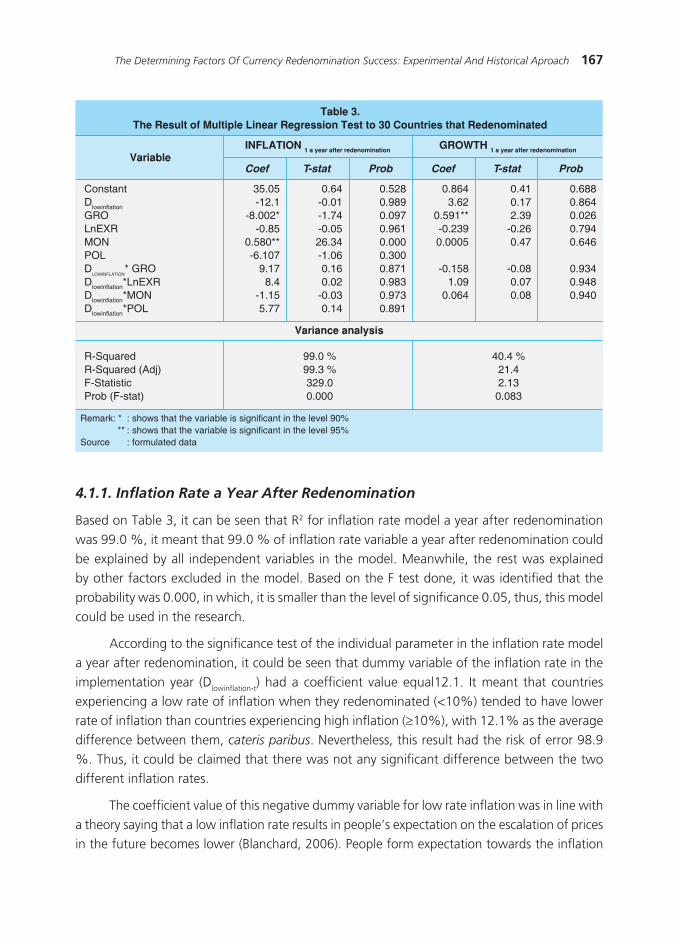
167The Determining Factors Of Currency Redenomination Success: Experimental And Historical Aproach
4.1.1. Inflation Rate a Year After Redenomination
Based on Table 3, it can be seen that R2 for inflation rate model a year after redenomination was 99.0 %, it meant that 99.0 % of inflation rate variable a year after redenomination could be explained by all independent variables in the model. Meanwhile, the rest was explained by other factors excluded in the model. Based on the F test done, it was identified that the probability was 0.000, in which, it is smaller than the level of significance 0.05, thus, this model could be used in the research.
According to the significance test of the individual parameter in the inflation rate model a year after redenomination, it could be seen that dummy variable of the inflation rate in the implementation year (Dlowinflation-t) had a coefficient value equal12.1. It meant that countries experiencing a low rate of inflation when they redenominated (<10%) tended to have lower rate of inflation than countries experiencing high inflation (≥10%), with 12.1% as the average difference between them, cateris paribus. Nevertheless, this result had the risk of error 98.9 %. Thus, it could be claimed that there was not any significant difference between the two different inflation rates.
The coefficient value of this negative dummy variable for low rate inflation was in line with a theory saying that a low inflation rate results in people’s expectation on the escalation of prices in the future becomes lower (Blanchard, 2006). People form expectation towards the inflation
Table 3.The Result of Multiple Linear Regression Test to 30 Countries that Redenominated
Variable
Variance analysis
Coef T-stat Prob Coef T-stat Prob
INFLATION 1 a year after redenomination GROWTH 1 a year after redenomination
Constant 35.05 0.64 0.528 0.864 0.41 0.688Dlowinflation -12.1 -0.01 0.989 3.62 0.17 0.864GRO -8.002* -1.74 0.097 0.591** 2.39 0.026LnEXR -0.85 -0.05 0.961 -0.239 -0.26 0.794MON 0.580** 26.34 0.000 0.0005 0.47 0.646POL -6.107 -1.06 0.300 D
lowinflation* GRO 9.17 0.16 0.871 -0.158 -0.08 0.934
Dlowinflation*LnEXR 8.4 0.02 0.983 1.09 0.07 0.948Dlowinflation*MON -1.15 -0.03 0.973 0.064 0.08 0.940Dlowinflation*POL 5.77 0.14 0.891
R-Squared 99.0 % 40.4 %R-Squared (Adj) 99.3 % 21.4F-Statistic 329.0 2.13Prob (F-stat) 0.000 0.083
Remark: * : shows that the variable is significant in the level 90% ** : shows that the variable is significant in the level 95%Source : formulated data

168 Bulletin of Monetary, Economics and Banking, Volume 17, Number 2, October 2014
based on the inflation being observed or the previous year inflation ( ), Mankiw (2003) label this as adaptive expectations. Past inflation influences future inflation expectation, Solow in Mankiw (2003) states that “we encounter inflation because we expect it, and we expect inflation because we encounter it”. To put it in other words, the escalation of past inflation influences the escalation of inflation expectation and eventually, it can cause actual inflation in the following year.
In countries that are implementing redenomination, they even tend to encounter money illusion where people make mistake in perceiving the nominal change or real. The policy of currency nominal value change along with high inflation rate will compound people to compare the previous real value and after the policy implementation. Blanchard (2006) also categorizes money illusion as the cost of inflation. Because of that, if there is a policy to change currency nominal when the inflation rate is high, sellers will take advantage of it to escalation the selling price because the people’s expectation on inflation has already been high due to the inflation rate currently happening and the escalation of those prices will be deceived by money illusion resulted from currency redenomination.
The significant variables influence inflation rate a year after redenomination with probability value below level of significance 10% were the economic growth in the year of redenomination implementation (GRO) and the growth of money in circulation in the same year (MON). The better the economic growth in the year of implementation is, the lower the rate of inflation in the following year will be. Meanwhile, the positive MON coefficient shows that the more money is circulating, so after redenomination, the inflation rate tends to increase. Other variables in the model, like the interaction between dummy condition low inflation rate and other variables didn’t have a significant influence. The result of this analysis could explain why some countries achieved low and stable inflation rate after redenominated their currency while others achieved different rate. The role of economic condition at the moment of redenomination becomes a very important thing to be taken into account because it can influence the economic condition after redenomination being implemented.
4.1.2. Economic Growth a Year After Redenomination
Regression model for the economic growth a year after redenomination had R2 value equal to 40.4%, meaning that the total variance in the data was explained 40.4% while the rest was explained by factors outside the model. F statistical test in this model could be seen from Prob (F-stat) equal to 0.083, it meant that the four independent variables significantly influenced the economic growth in the year after redenomination simultaneously in the 10% trust level.
In the regression model of the economic growth in the year after redenomination, dummy variable of inflation rate (Dlowinflation) had coefficient value equal to 3.62. It meant that a country with low inflation when redenomination was being implemented tended to have higher economic growth in the year after redenomination compared to countries with high
169The Determining Factors Of Currency Redenomination Success: Experimental And Historical Aproach
inflation. Yet, in this model Dlowinflation variable was not significant since it had 86.4% the risk of error or above 10% level of significance. The only significant variable influenced the economic growth in the year after redenomination was the growth of the year when redenomination was implemented. The higher the economic growth was, the higher the growth in the following year would be. In the mean time, other variables did not significantly influence the economic growth a year after the implementation. Again, this result presented that expectation played an important role in determining economic condition achievement of a country, especially the 30 countries that had redenominated.
4.2. Experiment Simulation Result of Posted Offer Market Transaction System
Causality direction between currency redenomination and economic condition is hard to determine, one of the ways of determining it is by doing an experiment or controlled trial. The experiment was done to see the responses towards redenomination policy, i.e. the omission of 3 zero digits in the nominal value of Rupiah towards the selling price, the number of transaction and the total number of transaction in rice commodity market with posted offer buying and selling system. The responses of that experiment also compared different influences of redenomination in some different economic conditions, like the inflation rate and the economic growth. This experiment simulation was done with the procedures explained earlier in the methodology section.
4.2.1. The Implication of Redenomination Policy Towards the Change of Selling Price in the Posted Offer Market System
Based on the experience of the countries that had redenominated, there are two possibilities that might happen after this policy implementation. The first is the goods price is controlled and stable and the second is that the price increases. The experiment simulation conducted showed that redenomination without considering economic conditions didn’t have a significant influence to the selling price. Before redenomination, the average of selling prices of all experimental group was Rp 7 498.2 and after redenomination, the average was Rp (new) 7.529 or Rp 7 529. This can be seen in Figure 8 below. Although they were not far different, there was a tendency of price escalation after redenomination. Nevertheless, for commodities whose elastic demands to prices, like car, after redenomination the selling price tends to decrease (Astrini, 2014).

170 Bulletin of Monetary, Economics and Banking, Volume 17, Number 2, October 2014
Figure 1. The Average of the Selling Price of Rice Commodity Before and After Redenomination
���������������������
����
����
����
����
�������������� ������� ������������ �������
���� �����
Nonetheless, it was necessary to see the price change difference after redenomination in different economic conditions like inflation rate and economic growth. This was intended to see whether different conditions resulted in different results or not regarding the price change resulted from redenomination. This difference was tested with Mean difference test, and the results are presented in Table 4. The table shows that redenomination had various effects to the price change, it depended on the economic condition accompanying it.
In the table it can be generally sees that from all different conditions, the selling price after redenomination in the low inflation condition either when it was combined with economic growth or when it was not, decreased or the change was negative in value. Meanwhile, the
Table 4. Mean Difference Test of the Change Percentage of Selling Price After Redenomination in Various Conditions
ConditionsPrice Change
percentage after redenomination (%)
variance(σ2)
T-Value P-Value
Low inflation and low growth -0.4559High inflation and low growth 1.259Low Growth and low growth 0.19594High Growth and low growth 0.60719Low inflation and Low Growth -0.5126High inflation and Low Growth 0.9045Low inflation and High Growth -0.3992High inflation and High Growth 1.6136Low inflation and Low Growth -0.5126Low inflation and High Growth -0.3992High inflation and Low Growth 0.9045High inflation and High Growth 1.6136
The same 1.44 0.090* The same 0.32 0.379 The same 0.69 0.263 The same 1.21 0.147 The same 0.06 0.478 The same 0.39 0.359
Ket: * significant in the level of level of significance 10% Source: formulated data
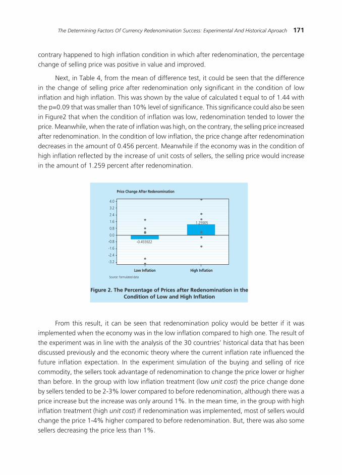
171The Determining Factors Of Currency Redenomination Success: Experimental And Historical Aproach
Figure 2. The Percentage of Prices after Redenomination in the Condition of Low and High Inflation
contrary happened to high inflation condition in which after redenomination, the percentage change of selling price was positive in value and improved.
Next, in Table 4, from the mean of difference test, it could be seen that the difference in the change of selling price after redenomination only significant in the condition of low inflation and high inflation. This was shown by the value of calculated t equal to of 1.44 with the p=0.09 that was smaller than 10% level of significance. This significance could also be seen in Figure2 that when the condition of inflation was low, redenomination tended to lower the price. Meanwhile, when the rate of inflation was high, on the contrary, the selling price increased after redenomination. In the condition of low inflation, the price change after redenomination decreases in the amount of 0.456 percent. Meanwhile if the economy was in the condition of high inflation reflected by the increase of unit costs of sellers, the selling price would increase in the amount of 1.259 percent after redenomination.
���������������������������������
���������
�������
���
���
���
���
���
���
����
����
����
����
������������������������
������� ������������
From this result, it can be seen that redenomination policy would be better if it was implemented when the economy was in the low inflation compared to high one. The result of the experiment was in line with the analysis of the 30 countries’ historical data that has been discussed previously and the economic theory where the current inflation rate influenced the future inflation expectation. In the experiment simulation of the buying and selling of rice commodity, the sellers took advantage of redenomination to change the price lower or higher than before. In the group with low inflation treatment (low unit cost) the price change done by sellers tended to be 2-3% lower compared to before redenomination, although there was a price increase but the increase was only around 1%. In the mean time, in the group with high inflation treatment (high unit cost) if redenomination was implemented, most of sellers would change the price 1-4% higher compared to before redenomination. But, there was also some sellers decreasing the price less than 1%.

172 Bulletin of Monetary, Economics and Banking, Volume 17, Number 2, October 2014
Meanwhile, if we compare the high economic growth and the low one, the price change after redenomination in those two conditions was not significantly different3. This can be seen in Table 4 above that the value of p was 0.379 (more than 10% level of significance). Nevertheless, it needs to be observed here that in either low or high growth, currency redenomination resulted in the selling price of rice commodity kept increasing, 0.195 and 0.607 % for each.
3 In the experiment simulation, the economic growth was reflected by the total number of sellers and buyers involving in the market of rice commodity. In the high economic growth, the economic subject in the market is 40% higher compared to the low growth.
Figure 3.Post-Redenomination Price Change percentage in different
inflation conditions and economic growths
����������������������������������
��������
��������� ���������
�
�
�
�
�
��
��
��
��������� ���������
�������
������� ���������� ����
������������ ���������
The highest price escalation after redenomination is experienced by a combination group of high inflation rates in high economic growths. In that group, redenomination causes the price of goods to rise as much as 1.61%. Compared to the percentage of price change in low inflation and similar economic growth, this change has the risk of failing as much as 14.7% (p-value=0.147) or less significant. This is shown in Figure 3 above. Nevertheless, this fact indicate that if redenomination is applied while experiencing high inflation and high economic growth at the same time, there is a tendency for sellers to raise the price in hop for perception bias or money illusion in the buyers. So the sellers will recieve higher income from the redenomination.
The experiment result shows that if sellers only have small profit margin, this happens when the inflation rate is high or seller’s unit cost is large, so the seller will raise the price post-redenomination in hope to get bigger profit than before. The sellers think that by raising the price they will get higher profit as well. On the contrary, if the seller had already got sufficiently large profit margin, with the relatively small unit cost, the seller will lower the price post-redenomination so that the goods will sell out more on the market. This is dine to avoid

173The Determining Factors Of Currency Redenomination Success: Experimental And Historical Aproach
unsold goods due to the high price. It can be stated that the redenomination policy has different influence for each sellers, depending on their characteristics pre-redenomination, whether they belong in the high inflation or low inflation group.
The result goes along with the research done by Hobijn et al. (2006) and Gamble et al.
(2002) where the Euro redenomination case, people had already percieve that the prices will get lower due to the removal of some digits from their previous currency although the real value of the goods itself is actually rising. The study done by Shafir et al. (1997) also shows the mistake people have done in counting the real value in economic transaction, due to only viewing the nominal value itself. These studies and the result shows that money illusion is common on economic subjects. The median difference analysis can also be used as benchmark of the difference in redenomination influence towards price change in different economic conditions, especially the inflation rate. So it can be seen how redenomination policy could bring a currency to a better or even worse state.
4.2.2. The Redenomination Policy Implication Towrds Transaction ammount change in Posted Offer Market System
Without concerning the economic condition, the amount of average transaction tends to decrease as much as 0.33 litre compared to the previous one. The decrease in total number of transaction response goes along with the increasing response of selling price post-redenomination. This fact suits the demand law in economic theory where the amount of goods request will decrease if there are any rising price. (Lipsey et al., 1995). Furthermore, in any economic condition, redenomination doesn’t have any different influence to the response
Table 5. The median test of Post-redenomination total number of transaction change percentage in different economic conditions.
ConditionsPost-redenomination total
number of transaction change percentage (%)
Manner(σ2)
T-Value P-Value
Low Inflation -4.2328High Inflation -3.3796Low Growth -1.8254High Growth -5.787Low Inflation and Low Growth -4.7619High Inflation and Low Growth 1.1111Low Inflation and High Growth -3.7037High Inflation and High Growth -7.8704Low Inflation and Low Growth -4.7619Low Inflation and High Growth -3.7037High Inflation and Low Growth 1.1111High Inflation and High Growth -7.8704
Similar 0.14 0.446 Similar 0.67 0.260 Similar 0.51 0.320 Similar 0.77 0.242 Similar 0.18 0.435 Similar 0.79 0.236
Source: Developed data
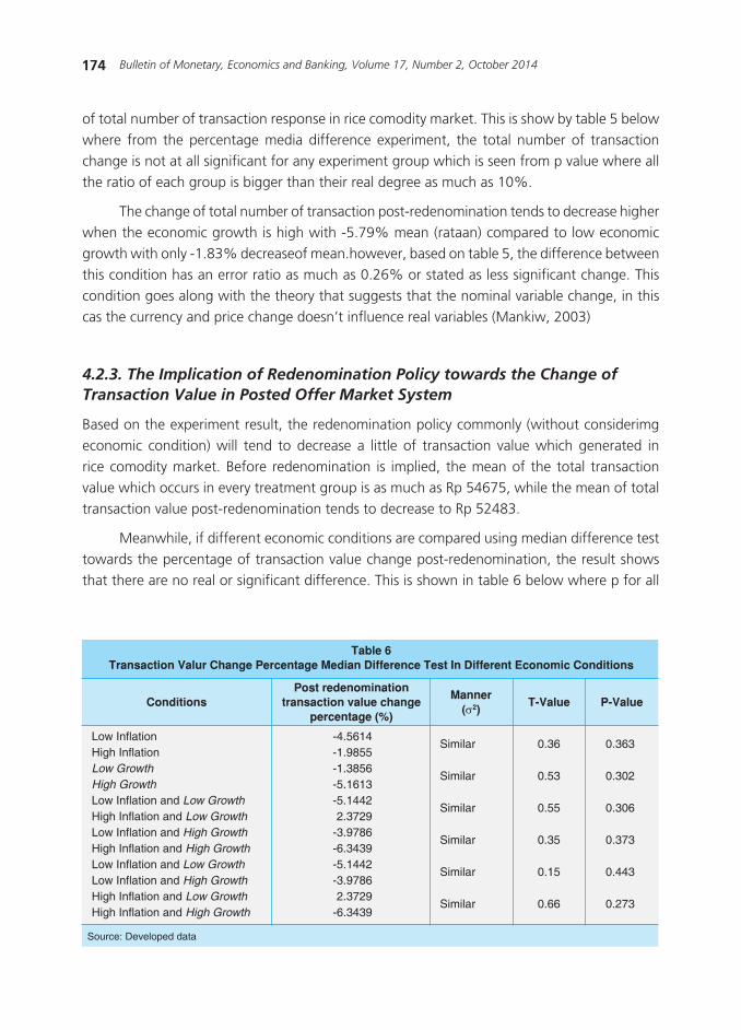
174 Bulletin of Monetary, Economics and Banking, Volume 17, Number 2, October 2014
of total number of transaction response in rice comodity market. This is show by table 5 below where from the percentage media difference experiment, the total number of transaction change is not at all significant for any experiment group which is seen from p value where all the ratio of each group is bigger than their real degree as much as 10%.
The change of total number of transaction post-redenomination tends to decrease higher when the economic growth is high with -5.79% mean (rataan) compared to low economic growth with only -1.83% decreaseof mean.however, based on table 5, the difference between this condition has an error ratio as much as 0.26% or stated as less significant change. This condition goes along with the theory that suggests that the nominal variable change, in this cas the currency and price change doesn’t influence real variables (Mankiw, 2003)
4.2.3. The Implication of Redenomination Policy towards the Change of Transaction Value in Posted Offer Market System
Based on the experiment result, the redenomination policy commonly (without considerimg economic condition) will tend to decrease a little of transaction value which generated in rice comodity market. Before redenomination is implied, the mean of the total transaction value which occurs in every treatment group is as much as Rp 54675, while the mean of total transaction value post-redenomination tends to decrease to Rp 52483.
Meanwhile, if different economic conditions are compared using median difference test towards the percentage of transaction value change post-redenomination, the result shows that there are no real or significant difference. This is shown in table 6 below where p for all
Table 6Transaction Valur Change Percentage Median Difference Test In Different Economic Conditions
ConditionsPost redenomination
transaction value change percentage (%)
Manner(σ2)
T-Value P-Value
Low Inflation -4.5614High Inflation -1.9855Low Growth -1.3856High Growth -5.1613Low Inflation and Low Growth -5.1442High Inflation and Low Growth 2.3729Low Inflation and High Growth -3.9786High Inflation and High Growth -6.3439Low Inflation and Low Growth -5.1442Low Inflation and High Growth -3.9786High Inflation and Low Growth 2.3729High Inflation and High Growth -6.3439
Similar 0.36 0.363 Similar 0.53 0.302 Similar 0.55 0.306 Similar 0.35 0.373 Similar 0.15 0.443 Similar 0.66 0.273
Source: Developed data

175The Determining Factors Of Currency Redenomination Success: Experimental And Historical Aproach
comparisons between (economic conditions) groups are bigger compared to 10% real degree (taraf nyata).
4.3. People’s Perspective Towards The Redenomination Policy
To find out the people’s opinions towards the impact from the policy of rupiah’s redenomination in Indonesia, thus executed surveys in form of interviews and polls with questionnaires to 168 respondents in Bogor during May-June 2013.
4.3.1. Redenominasi The Governmen’s Ability to Control Inflation Post-Redenomination
Based on the simulation of economic experiments result, a tendency occured where the prices of goods will increase after redenomination. The survey data based on people’s perspective shows similar result with the previously mentioned experiment result, it is seen that most of the respondents or as many as 53% are not sure that the government could control the inflation steadily post-redenomination. These respondents have several reasons, mostly because they believe that the prices, mainly basic needs(kebutuhan pokok) will rise post-redenomination. This is based on the experience where prices tend to rise during economic fluctuations or major events such as religious holidays, or national disasters. The redenomination policy could also be included as one of the major events that will change people’s behavior especially in purchases and sells transactions. However, as many as 32% respondents still believe that the government still can control the inflation post-redenomination, and the last 15% admitted that they are unaware. The result can be seen in the Figure below.
Figure 4.People’s Trust Level In Government’sControl Ability Post Redenomination
����������
���������
�������
��������������������

176 Bulletin of Monetary, Economics and Banking, Volume 17, Number 2, October 2014
This survey result shows that the inflation expectation post-redenomination is quite high. According to Dornbusch et al. (2004) only a credible policy could change the inflation expectation to be appropriate with what the government targeted. The respondents who don’t believe the government in controlling the inflation post-redenomination argued that Indonesia’s economic condition is not yet ready to face the redenomination policy due to the lack of public dissemination and education regarding the policy and the lack of introduction to the new type of currency to society. Meanwhile, the uncertainty of redenomination policy will also give psychological effect, especially the low trust to the government in economic improvement. While the respondents who believe that the government can control the inflation post-redenomination argued that rupiah’s redenomination will not significantly impact Indonesia’s economy, namely in the inflation rate. The argued that the controllable inflation rate by the government has no relation to redenomination policy. While those who are unaware, mostly haven’t know anything about the redenomination policy yet.
4.3.2. Consumption Pattern Change Post-Redenomination
The anxiety of high inflation post-redenomination, will surely impact the consumption pattern change in society. Namely buying more real assets than before,with the hope of the wealth owned does not decrease due to the inflation. Nevertheless, from the survey to 168 respondents, it is revealed that only 38.10 percent thinks that it is better to buy real assets post-redenomination as shown in Figure 5 below. While the majority of 59.52% tend to choose not to change their consumption pattern, this is due to the fact that redenomination will only change the nominal writing of a currency, so that the prices of goods will not significantly change. Many respondents understood that redenomination will not change the real value of goods, money, wealth, and people’s purchase force (daya beli). While they also argued that there will be no influence between the policy and inflation rate change.
Several respondents who chose to buy more real asset post-redenomination stated that the price of real assets like gold psychologically will look cheaper. Besides, the real assets price will rise in the near future anyway, so they feel it safer to store their wealth in the form of real asstes. While the respondents who chose to buy more consumption good post-redenomination are as many as 2.38%, they stated that the prices will become a lot cheaper so their consumption rate will increase. They consider that redenomination will reduce the value of money so the money they have will be better spent than store. Based on this survey, it can be seen that most respondents are not affected by the money illusion from redenomination, only 2.38% are affected by it.

177The Determining Factors Of Currency Redenomination Success: Experimental And Historical Aproach
4.3.3. Rupiah’s Exchange Rate Reinforcement Post-Redenomination
The redenomination policy by removing 3 digits in rupiah’s currency mainly aim to give an impact of rupiah being equal or even stronger than other currencies, concidering rupiah is now the third country with the highest exchange rate. The interview result to 168 respondents shows that 37 respondents answered that the redenomination policy will not strengthen the value of rupiah since the exchange rate (apreciation and depreciation) will be influenced more by other factors outside the change of nominal value of the currency, mainly by remittance scale (neraca pembayaran). This can be seen in Figure 6 below.
Figure 5.Consumption Pattern Change Post-Redenomination
�����
�
�����
�����
�������������������
��� �������������������
������������� ����������������������
�����
������
������
Figure 6. People’s Perspective Towards Rupiah’s Exchange Rate Amplification Post-Redenomination
����
����
����
��������������������

178 Bulletin of Monetary, Economics and Banking, Volume 17, Number 2, October 2014
Meanwhile, as many as 33% percent of respondents answered that the redenomination policy will strengthen rupiah’s nominal calue, the reason is because th rupiah’s nominal value will approach that of US dollars so that rupiah will seem stronger than before and will improve the society’s trust in keeping rupiah. While 30% of the respondents answered unaware about the connection between redenomination and rupiah’s exchange rate.
V. CONCLUSION
Based on several analysis results which have been done using historical data approach, economic experiments, and interviews along with the discussion explained earlier regarding redenomination policy, therefore this research concludes:
If the success of the implication od redenomination policy is measured by the low inflation rate and the high economic growth, the success of redenomination tends to be influenced by economic condition of the country when it applies redenomination. Countries which applies redenomination during low inflation rate (<10%), they will have lower inflation rate after a year compared to other countries that applies redenomination while having high inflation rate (≥10%). Meanwhile, the economic growth post-redenomination could escalate if the economic growth is high wile apllying redenomination.
Based on the result of experiment regarding rice transaction in posted-offer market system, the rise or fall of price post-redenomination significantly influenced by the inflation rate condition along with it. During high inflation, redenomination policy will excalate selling price. On the contrary, the selling price will decrease when redenomination is applied during low inflation. Meanwhile, the economic growth does not affect the selling price change post-redenomination. From the result, it can be concluded that with different economic conditions, the redenomination policy does not significantly affect the change of total number of transaction and the total transaction which occured in the market. However, if the economic condition is ignored, redenomination will commonly cause selling price excalation, total number of transaction decrease, and transaction value decrease. The survey revealed most of the respondents do not believe that the government could control the inflation post-redenomination. Redenomination will neither influence the society’s consumption pattern and they do not believe that redenomination will strengthen the rupiah’s exchange rate.
Seen from the research result, the important factor in the implementation of redenomination is the economic condition during that time. It will be better if the redenomination is applied during a steady and good economic condition, like low inflation rate and high economic growth. The public dissemination of the redenomination policy to society should be done previously intensively and consistently to give clear information to the public regarding the policy.

179The Determining Factors Of Currency Redenomination Success: Experimental And Historical Aproach
In addition, the author suggests that further research needs to be done which focused on the impact of redenomination directly to economic condition. Other than that, further research with similar economic experiment needs to be done to other transaction systems besides posted-
offer which are decentralization and double auction. That research should preferably use different experiment subjects for every repetition and treatmen, so that the experiment subject does not go through the same encounter as before. This is meant to get relatively better experiment results. The next researches is expected to expand the coverage of response influence and add other factors, so they can give more vivid image regarding the redenomination policy towards economy. The experiment simulation will be better if connected computers are used between experiment subjects, to minimize the influence of other factors outside the treatment.

180 Bulletin of Monetary, Economics and Banking, Volume 17, Number 2, October 2014
REFERENCES
Amir, A. “Redenominasi Rupiah dan Sistim Keuangan”, Jurnal Paradigma Ekonomika. Vol. 1, No. 4 Oktober 2011.
Astrini, Danti. “Kajian Dampak Redenominasi terhadap Perekonomian dengan Metode
Percobaan Ekonomi”, Tesis, Sekolah Pascasarjana, Institut Pertanian Bogor, 2014.
Blanchard, O, (2006), Macroeconomics Fourth Edition, Pearson Prentice Hall.
Dornbusch, R, Fischer S, dan Startz R, (2004), Macroeconomics Ninth Edition, McGraw Hill, New York.
Gamble, A, Garling T, Charlton J, & Ranyard R. “Euro Illusion”, European Psychologist 7, 2002, 4: 302-31.
Hobijn, Bart, F. Ravena, dan A. Tambalotti. “Menu Costs at Work: Restaurant Prices and the Introduction of the Euro”,The Quarterly Journal of Economics, 2006, 121 (3): 1103-1131.
Iona, D. “The National Currency Re-denomination Experience in Several Countries: A Comparative
Analysis”, International Multidisciplinary Symposium Universitaria Simpro, 2005.
Juanda, B. “Percobaan Ekonomi untuk Mengkaji Pengaruh Informasi Serta Jumlah Penjual dan Pembeli dalam Transaksi Pasar”, November 2000, Jurnal Ekonomi Vol. 7, III, Universitas Borobudur.
_______________. “Ekonomi Eksperimental untuk Pengembangan Teori Ekonomi dan Pengkajian Suatu Kebijakan”,Di dalam: Orasi Guru Besar IPB, 25 September 2010.
_______________. “Experimental Economics in Indonesia: Lesson Learned and Best Practices”, Di dalam: Workshop on Experimental Economics, Bogor 6 September 2012.
Juanda, B, N. Fitri, F. Fardilah, dan M.P.D. Manik, (2011),“Analisis Perbandingan Dampak Kebijakan Menyelamatkan Bank Century dengan kebijakan Menutup Bank Century dengan Metode Eksperimen”, Departemen Ilmu Ekonomi, FEM-IPB, Bogor.
Kesumajaya, I.W.W. “Redenominasi Mata Uang Rupiah Merupakan Bagian dari Tugas Bank Indonesia untuk Mengatur dan Menjaga Kelancaran Sistim Pembayaran di Indonesia”,GaneC Swara Vol. 5 No.1, Pebruari 2011.
Lianto, J dan Ronald Suryaputra. “The Impact of Redenomination in Indonesia from Indonesian Citizens’ Perspective”, Procedia - Social and Behavioral Sciences 40 (2012): 1 – 6.
Lipsey, R.G, P.N Courant, D.D Purvis, dan P.O Steiner,(1995),Pengantar Mikroekonomi Jilid Satu
Edisi Kesepuluh. Binarupa Aksara. Jakarta. Terjemahan dari: Economics 10th ed.

181The Determining Factors Of Currency Redenomination Success: Experimental And Historical Aproach
Mankiw, N.G,(2003),Teori Makroekonomi Edisi Kelima. Erlangga. Jakarta. Terjemahan dari: Macroeconomics 5th Edition.
Matjik, A.A, dan I.M. Sumertajaya, (2002), Perancangan Percobaan dengan Aplikasi SAS dan
MINITAB Jilid I Edisi Kedua. IPB Press. Bogor.
Marques, J.F dan Dehaene, S.“Developing Intuition for Price in Euros”, Journal of Experimental Psychology 10, 2004, 3: 148-155.
Mehdi, S dan Motiee Reza. “An investigating Zeros Elimination of the National Currency and Its Effect on National Economy (Case study in Iran)”, European Journal of Experimental Biology, 2012, 2 (4):1137-1143.
Mosley, L. “Dropping Zeros, Gaining Credibility? Currency Redenomination in Developing Nations”, 2005 Annual Meeting of The American Political Science Association, Washington DC.
Shafir, E, P. Diamond, dan A. Tversky. “Money Illusion”, The Quarterly Journal of Economics (May 1997) 112 (2): 341-374.
Suhendra, E dan S.W. Handayani. “Impacts of Redenomiantion on Economics Indicators”, International Conference on Eurasian Economies, 2012.
The World Bank. “World Development Indicators 2012”, 2012.
Wibowo. B. “Ilusi Nilai Uang Redenominasi”, Harian Bisnis Kontan, Kamis 21 Februari 2013.

182 Bulletin of Monetary, Economics and Banking, Volume 17, Number 2, October 2014
This page intentionally left blank
197Foreign Exchange Expectations in Indonesia: Regime Switching Chartists & Fundamentalists Approach
Foreign exchange expectations in indonesia: regime switching chartists & Fundamentalists approach
Ferry Syarifuddin1
Noer Azam AchsaniDedi Budiman Hakim
Toni Bakhtiar
This paper investigates the effect of central bank intervention using a heterogeneous expectations
exchange rate model. We apply Markov switching approach on daily USD/IDR exchange rate, intervention
data of Bank Indonesia, from 2006 to 2012. The results support both chartists and fundamentalist regimes,
and confirm the two regimes to be persistent. Moreover, the intervention of Bank Indonesia on foreign-
exchange is capable to drive the USD/IDR to its fundamentalist rule. However, on Bank Indonesia efforts
to exert a stabilizing effect of foreign exchange interventions, the result is inconclusive.
abstract
Keywords: Exchange rates, foreign-exchange intervention, switching regression
JEL Classification: F31, E52, C24
1 Post-graduate student, Bogor Agricultural University, Graduate Program of Business & Management, (Corresponding author, [email protected]). Noer Azam Achsani ([email protected]), Dedi Budiman Hakim ([email protected]), Toni Bakhtiar ([email protected]) are lecturer in Bogor Agricultural University, Graduate Program of Business & Management.

198 Bulletin of Monetary, Economics and Banking, Volume 17, Number 2, October 2014
I. INTRODUCTION
According to the postulate of impossible trinity, a free floating exchange rate regime will be adapted by a country with free capital mobility and independent monetary policy. Indonesia is one of country that adapts it. With the free floating exchange rate and a size of small open economy, the fluctuation of Rupiah’s rate depends strongly on the capital flows particularly the short run. In foreign exchange market, the capital flows is a reaction of the buy or sell activities from the market players, which is categorized in two groups. The first group is fundamentalists who buy or sell foreign exchange based on their exchange rate expectation following the fundamental economic condition. The second group is chartist who buys or sells foreign exchange based on their exchange rate expectation following the previous exchange-rate behavior. These two groups determine the market exchange-rate.
Sometimes the exchange rate moves beyond their fundamental value, and this requires the central bank to intervene to drive the exchange rate back to its long-run fundamental value. Many empirical literatures including Almekinders and Sylvester (1996), Frenkel (2004), Ito and Yabu (2007), and Neely and Weller (2001) suggested the foreign-exchange intervention policy was to reduce the exchange rate misalignment or undesired fluctuations.
We can distinguish two types of forex intervention; first is a non-sterilized foreign-exchange intervention where the decision of monetary authority to buy or to sell foreign exchange affects the monetary base, interest rates, market expectations and the exchange rate. Secondly, a sterilized-foreign-exchange intervention is policy by monetary authorities to “defend” the value of their currency or the domestic money supply despite external shocks or other changes, including the flow of capital out of the relevant area.
With central bank policy, we expect the exchange rates to stay in desired level and stable. Nevertheless, besides relying on central bank policy to stabilize the exchange rate, financial agents are sometimes actively hedging the exchange rate in order to avoid losses due to exchange rate fluctuations. Röthig, Semmler, and Flaschel (2005) argued that the negative effect of exchange rate on the balance sheet can be eliminated by risk management like hedging. Hedging generally conducts by forward transactions, swaps, NDF etc.
This paper analyzes the microstructure of foreign exchange market players (fundamentalists and chartists) in determining exchange rate. We expect this approach will be able to overcome failures of numerous empirical studies based on asset market approach on explaining the short term movements of exchange rate (Lewis, 1995 and Taylor, 1995. This paper adopts the exchange-rate microstructure approach called ‘noise trading’ channel pioneered by Hung (1997) and the coordination channel Reitz and Taylor (2008), and Taylor (2004), (2005). Ahrens and Reitz (2003) perform empirical study regarding to this issue and their result provide evidence that the heterogeneous expectations exchange rate model is able to explain daily German-US forward rates. Further research by Maatoug, Fatnassi, Omri (2010) finds that both regimes (fundamentalists and chartists) are persistent in Australia. However he finds that the

199Foreign Exchange Expectations in Indonesia: Regime Switching Chartists & Fundamentalists Approach
fundamentalist’s regime is riskier and when the RBA was not active in the foreign exchange, the fundamentalists were disappeared. Other study using Markov switching approach by Brunetti, Mariano, Scotti (2007) in Southeast Asia, finds that real effective exchange rates, money supply, stock index returns, are important variables to identify turbulence and ordinary periods.
To investigate different forecasting strategies by the players, the impact of central bank intervention is investigated by applying a heterogeneous expectations exchange rate model. The approach is also evaluated by including central bank intervention policy to drive exchange rate to its long-run fundamental value. Foreign-exchange interventions may influence the forecasting rules of chartists and fundamentalists, thereby altering the proportion of the two groups in the foreign exchange market. A central bank intervening in the foreign exchange market is considered effective if the exchange rate is driving closer to its fundamental value. Generally, foreign-exchange intervention may as well improve the performance of expectations based on fundamentals, especially when central banks try to correct current exchange rate misalignments. Following Frankel and Froot (1986) the excess demand/supply for foreign currency is assumed to be a function of the relative success of chartist and fundamentalist forecasting techniques. As is stated above the performance of chartist or fundamentalist predictions is expected to be temporarily improved by central bank intervention.
This research furthermore re-examines the effects of foreign-exchange intervention on exchange rate volatility within the heterogeneous groups in the foreign exchange market. These studies suggested new channels through which sterilized intervention may be transmitted: the noise trading channel (Hung, 1997), which assume that the noise traders will determine the exchange rate by flow of market equilibrium, and that the central bank should intervene in highly volatile market periods and keep its interventions secret (Reitz, 2002).
This empirical research is done by applying the Markov regime-switching approach originally proposed by Hamilton (1989) to daily Bank Indonesia data from 2006 to 2012. Considering the results of Neely and Weller (2001) intervention data is used only to construct a dummy variable distinguishing between intervention and no-intervention periods. Statistically significant estimates of dummy coefficients lead to the conclusion that an impact of central bank intervention on exchange rate expectation cannot be rejected.
The remainder of the paper is organized as follow. Section 2 describes the theory and literature study, followed by Research Methodology in section3. Our main empirical results concerning intervention effectiveness are reported in Section 4, before the final section (5) concludes.

200 Bulletin of Monetary, Economics and Banking, Volume 17, Number 2, October 2014
II. THEORY
2.1. The Microstructure of the Forex Market and Monetary Policies
In macro perspective, foreign exchange level should reflect the fundamental economy condition. As described so far, the determinants of the exchange rate like inflation, productivity, interest rate, etc. categorized as fundamental factors which significantly affect long-run exchange-rate. Furthermore, news related to the fundamental factors such as statistic announcements of money supplies, trade balances, or fiscal policies is received by the market, and the exchange rates will also change to reflect this news. However, there is also significant issue regarding foreign-exchange microstructure which also determines exchange rates. Understanding the “market microstructure” allows us to explain the evolution of the foreign exchange market, in which foreign exchange traders adjust their foreign-exchange purchase or sale. In addition to macroeconomic indicators news, there also exists private information from which some traders know more than others about the current state of the market.
As illustrated in Figure 1, exchange rate is determined by two groups according to different approaches of expectations; the fundamental analysis and the chartist analysis. The classification was proposed previously by Frankel and Froot (1986, 1990), and has been enhanced among others by Ahrens and Reitz (2003), Reitz (2002), Westerhoff (2003), Wieland and Westerhoff (2005). In this diagram, the market exchange-rate is built by combining fundamentalists and chartist’s exchange-rate expectation adjusted by their own proportion in the foreign-exchange market. In the period of misaligned exchange-rate from desired value, central bank will enter the market to re-adjust the exchange rate to its desired level or mitigate the short-term fluctuations.
Figure 1.Fundamentalist-Chartist FX Expectation Mechanism
Source: Own Elaboration
Central Bank’sFX Intervention
FX Supply FX Demand
FX Domestic Market
FX EquilibriumUSD/IDR
Fundamentalist-ChartistFX Expectation
201Foreign Exchange Expectations in Indonesia: Regime Switching Chartists & Fundamentalists Approach
The global financial market has been pushing the financial market in emerging countries to integrate. As return of assets offered is often higher than ones in advanced financial market, the asset return including the exchange rate becomes more volatile. This condition is not accepted by most central banks as it will ignite greater uncertainty in their financial market. Some reasons include that a large movements in the real exchange rate away from medium-run equilibrium are costly, and secondly, there is imperfect capital mobility/asset substitutability. To overcome this phenomenon, most central banks in emerging market economies implement various monetary policies. The most popular ones are sterilized intervention and short-term policy rate. This opens up the fortuitous possibility that policymakers may be operating in a two-target, two-instrument world.
Lesson learned from previous financial crises, push central banks to maintain stable consumer prices if they are to achieve sustained and stable growth. Therefore, the central banks need more policies than just the policy interest rate such as foreign-exchange interventions. Lesson from crises taught that significant balance-sheet mismatches caused by exchange-rate misalignment, is not optimal. Thus, it is not wise to ignore possibly large deviations of the exchange rate from its medium-run equilibrium, even in an Inflation Target which requires floating exchange-rate system. The undesired exchange rate fluctuations might be response shortly by foreign-exchange intervention. On the contrary, reacting to such changes can deliver better economic outcomes under IT than benign neglect of the exchange rate (Stone, Roger, Shimizu, Nordstrom, Kisinbay, Restrepo, 2009). In this regard, beside two instruments (i.e. short-term policy interest rate and foreign-exchange intervention), there are potentially two policy targets: inflation and the exchange rate to be implemented in order to achieve sustainable economic growth.
Volatility in foreign exchange rates can disrupt domestic economy through deteriorating imports and exports performance, decreasing cross-border investment and funding, and threaten the stability of domestic prices through changes in prices for imported or exported goods (passed-through power of exchange rate to inflation). As a result, this could affect the domestic economy and even the economies of trading partners abroad. Therefore, the monetary authority even with ITF should manage the exchange rate to support the achievement of domestic price stability and domestic economy by applying monetary policies such as foreign exchange intervention. While many central banks objectives are to set the optimal level of foreign-exchange that support price stability achievement as well as to mitigate exchange-rate volatility, however, others prefer to limit exchange rate volatility rather than to meet a specific target for the level of the exchange rate. Beyond on that, most central banks admit that domestic interest is still the main reason why they enter the foreign-exchange market in a sustained basis. For example as summarized in BIS publication (2006), major emerging central banks in Asia perform selling intervention to halt the continuing their currency appreciation between the end of 2001 and the end of 2004. As a consequence, global foreign exchange reserves grew by over US$ 1600 billion, reflecting reserve accumulation by emerging market

202 Bulletin of Monetary, Economics and Banking, Volume 17, Number 2, October 2014
economies. This phenomenon shows the emerging central banks was actively enter the foreign exchange market to avoid their undesired appreciation of their currencies as it would harm their export competitiveness/domestic economy.
On the other hand, some central banks have different views on exchange rate. They conversely prefer to stay behind from the foreign exchange intervention such as few developed countries have actively intervened within the last decade. There are some reasons behind that decision. One of them suggests foreign exchange intervention policy is not good for the economy where unbalances exist. Letting the exchange rate fluctuate freely is a sign of economic rebalancing is working. In this case, the dynamics of the exchange rate is a functioned as automatic stabilizer for the economy. This argument is elaborated in the studies by Calvo and Reinhart (2000) which concludes the foreign exchange intervention is a kind of fear of floating phenomenon. BIS (2006) summarize the reasons why developed countries no longer intervenes their foreign-exchange market actively. BIS suggest that the instrument is only effective if regarded as additional policy interest rate. Another reason implied that large-scale intervention can undermine the stance of monetary policy independence. The last reason is that private financial markets have enough capacity to absorb and manage shocks - so let the market determine the exchange rate.
Many economists are interested to see the effectiveness of the exchange rate intervention conducted by the central bank to stabilize the exchange rate. However, the existing views differ about the effectiveness of this intervention on stabilizing the exchange rate. Taylor (2004) examines the effectiveness of the exchange rate intervention by using Markov switching model on dollar-mark data during the period of 1985-98. In his conclusion, Taylor shows that the intervention increase the probability of stability when the rate is misaligned, and that its influence grows with the degree of misalignment. However, intervention within a small neighborhood of equilibrium will result in a greater probability of instability.
Beine, Grauwe, and Grimaldi (2009) investigated the effect of sterilized intervention in a noise trading channel with two states Markov switching model. Using biweekly data, they found that interventions increase the weight of fundamentalists in the foreign exchange market and therefore exert stabilizing influence on the exchange rate. The fundamentalist behavior tends to stabilize the market while the presence of chartists may cause destabilization. Other study by Dominguez (1998) explored the effect of foreign exchange intervention by the G-3 central banks (US, German, and Japanese) on the behavior of exchange rates over the 1977-1994 periods. The results indicate that intervention operations generally increase exchange rate volatility.
As discussed previously, the microstructure approach of exchange rate studies suggested two new channels through which sterilized intervention may be transmitted. In this regards, foreign-exchange intervention influence the expectations of foreign-exchange traders which are defined as fundamentalist and chartists. In this case, Frankel and Froot (1988) developed a model incorporate both players which is used to forecast the exchange rate expectations by

203Foreign Exchange Expectations in Indonesia: Regime Switching Chartists & Fundamentalists Approach
them. The fundamentalist approach forecasts exchange rate expectation by the fundamentalists based upon economic fundamentals, whereas the chartist approach forecasts exchange-rate expectation by chartists based upon the past behavior of the exchange rate. Furthermore, this model is developed by Vigfusson (1996) by implementing the Markov regime-switching model, in which explains the Chartist and Fundamentalists (C&F). He also suggests that using MA chartist model appears to do much better the AR chartist model. In this approach there are two rules in which two forecasting equations of both chartist and fundamentalist set up to estimate foreign exchange expectations. In each equation, C&F model placed the time-varying weight.
Further research from Reitz (2002) analyzed the exchange rate market player’s behavior and also investigated the impact of central bank intervention to their exchange rate expectations. Reitz propose a generalization of the noise trader transmission mechanism to examine the impact of central bank intervention on exchange rates. Within heterogeneous exchange rate expectations model, the policy intervention suppose to support either the chartist or the fundamentalist forecasts, which drive the portfolio managers to adjust their foreign currency positions. He tests the model by applying daily US-dollar/DEM forward rates and intervention data of the Deutsche Bundesbank and the Federal Reserve from 1979 to 1992. He finds the performance of the simple chartist trading rules was strong whenever the central bank intervened on the foreign exchange market. Instead, the result of fundamentalist approach was worse.
In Australia, the RBA’s approach to foreign exchange market intervention has evolved since the floating of Australian dollar in 1983. This is particulary because the foreix market in Australia has developed and on the other hand, the market participants are better equipped on managing their foreign exchange risk. Over time, the intervention on foreign exchange market becomes much less frequent and targets specific period when the market disfunction occur. Infact, during the 2008 crisis, the RBA has suspended the foreign exchange intervention.
2.2. A Basic Chartist-Fundamentalist Model for the Exchange Rate
In this paper, the foreign exchange equilibrium is determined by the interactions of two market players; the fundamentalist and the chartist, both with their own expectation on exchange rate. The chartists use technical analysis by exploring the historical data to forecast the exchange rate in the future. On the other hand, the fundamentalists base their forecasts on the assumption that the exchange rate will move around and will converge to its fundamental value.
We construct basic model following Maatoug, Fatnassi, Omri (2010: 30-34) and Reitz (2002: 3-7). Fundamentalists forecasting rules and Chartists forecasting rules can be expressed, respectively, as follow:
(1)
(2)

204 Bulletin of Monetary, Economics and Banking, Volume 17, Number 2, October 2014
where: r
f,t = the forecasted value of the exchange rate return rt by fundamentalists
θ = a speed of adjustment for fundamental rulef
t-1 = lagged fundamental exchange rater
c,t = the forecasted value of the exchange rate return rt by chartistsψ = speed of adjustment for the chartists forecasting ruleЄ
c,t = the error term of chartists
Єf,t = the error term of fundamentalists
To solve the model, one can apply the Markov regime-switching technique initially introduced by Hamilton (1989: 357-384) and later developed by, among others, Engel (1994: 151–165) and Dewachter (1996: 405-407). In Markov switching model, the dynamics of the exchange rate is governed by unobserved state variable or a latent variable l
t (l
t = c for chartist regime lt = f for fundamentalists). The indicator regime l
t is parameterized as a first order Markov
process and is driven by first-order transition probabilities. The transition probabilities across the two regimes could be expressed as:
(3)
(4)
(5)
(6)
These probabilities are constant over time. In this specification, p is the probability to remain in the fundamentalist regime, and q in the chartist regime.
III. METHODOLOGY
3.1. Markov Switching Approach
As is stated in Clarida, Sarno, Taylor, Valente (2001: 61-83) the Markov regime - switching model is a natural candidate to characterize exchange rate behavior. In this model, the conditional mean of the exchange rate (µ
t), the conditional variance (h
t), changes of exchange rate (∆et) are
allowed to follow two different regimes–a chartist and a fundamentalist regime-represented by an unobservable state variable S
t. The regime indicator S
t is parameterized as a first-order
Markov process, where the transition probabilities (P for fundamental regime and Q for chartist regime), follow the typical Markov structure:

205Foreign Exchange Expectations in Indonesia: Regime Switching Chartists & Fundamentalists Approach
Thus, under conditional normality, an observed realization ∆et is presumed to be drawn
from a N(µ0t,h
0t) distribution if S
t = 0, whereas ∆e
t is distributed N(µ
1t,h
1t). The evolution of the
log first differences of exchange rates can there for be written as
(7)
(8)
Where εt is an i.i.d. standard normal variable. The parameter estimation of the mean (µ
t)
and variance (ht) equations in the regime switching model are derived from maximization of
the log-likelihood function
p1t = Pr (S
t = 1 | Φ
t-1) is the probability that the analyzed process is in regime 1 at time
t and is updated by means of Bayesian inference using information available at time t-1. Therefore, p
1t and (1-p
1t) can be regarded as weights assigned to regime dependent forecasts
resulting from a rational learning process as outlined in the theoretical exchange rate model. For comparison purposes, this research first specifies the mean equations without taking into account foreign exchange market activities of central banks. However, the important results of the study are derived from mean equations that include intervention dummies as it is done in the second specification.
3.2. The Chartist-Fundamentalist (C & F) Model Specification
This paper applies the Markov-switching approach on exchange rate expectation by fundamentalists and chartists in Indonesia as suggested by Reitz (2002). This paper will augment the basic model with some contemporaneous variables beside exchange-rate return and exchange-rate intervention with other variables such as NDF return and CDS. These augmented variables are used as they may have significant impact on exchange-rate behavior.
In the standard chartist and fundamentalist (C&F) model originally suggested by Frankel and Froot (1986: 24–38), the (log of the) exchange rate S
t is driven by the decisions of portfolio
(9)

206 Bulletin of Monetary, Economics and Banking, Volume 17, Number 2, October 2014
(10)
(11)
(12)
(13)
managers. In his model, foreign-exchange players buy and sell foreign currency in response to changes in their expected rate of changes and a set of contemporaneous variables included in a vector z
t. Thus, the exchange rate is written as:
where the vector of elasticity of the contemporaneous variables (β) and the elasticity of exchange rate expectation (a) should be constant overtime. Regarding to Frankel and Froot (1986: 24–38), it is assumed that portfolio managers generate their exchange rate expectations using a mixture of chartist and fundamentalist forecasts:
The parameter ωt, denoting the weight given to fundamentalist views at date t, is
dynamically updated by the portfolio managers in a rational Bayesian manner:
With:
Where ω*t-1 is the ex-post calculated weight that must have been assigned to fundamentalist
forecast in order to predict the current exchange rate change accurately. The value of δ reflects the extent to which portfolio managers enclose new information in this adaptive process and proves responsible for the exchange rate dynamics. Since portfolio managers always maintain a positive weight for both chartist and fundamentalist forecasts, ∆ω has to be restricted so that stays in the range between 0 and 1. To make sure that the empirical analysis remains tractable, another feedback rule is introduced. Similar to Lewis (1989: 79–100), portfolio managers are supposed to optimize the weight assigned to fundamentalist forecasts by means of a Bayesian learning process:
Where and i s dens i t y funct ion of forex return, both for chartists and fundamentalists respectively. Concerning the
207Foreign Exchange Expectations in Indonesia: Regime Switching Chartists & Fundamentalists Approach
expectation formation fundamentalists have in mind some kind of long-run equilibrium , to which the exchange rate reverts with a given speed θ over time, i.e.:
According to fundamentalist, foreign-exchange expectation by the exchange-rate traders can be moved as distributed symmetrically around its fundamental value . Although several research uses PPP as proxy of exchange-rate fundamental value, this paper uses that the fundamental value as described by uncovered interest parity (UIP). The model above explains that market exchange-rate will converge to its fundamental value in the long run. A study using PPP by Takagi (1991) provides evidence there is a valid relationship between market exchange-rate and fundamental exchange rate only in the long run implying low values for θ. This view is also supported by Taylor and Peel (2000) and Taylor (2001) showing that due to its nonlinear dynamics the exchange rate reverts to the PPP level, but only in the long run. Furthermore, PPP or UIP as a measure of the fundamental exchange rate e
t seems to be
suitable for the investigation of central bank intervention, because monetary authorities have used it as a target level (Dominguez and Frankel, 1993).
If market exchange rate does not converge to its fundamental value in the long run, central banks will enter the foreign exchange market. The efforts of the central banks on foreign exchange markets can be called effective, if the adjustment of the exchange rate (θ) to its long run equilibrium is accelerated.
This implies that the observed reversion of the exchange rate to PPP or UIP – denoted by - is driven by fundamentalist speculation, central bank intervention, NDF rate and CDS rate.
Denoting the influence of foreign exchange intervention/monetary policy by , NDF by and CDS by ωθ, this research can formulate as a function of a 0,1- Exchange-rate Intervention dummy I
t, NDF
t and CDSt as follows:
(14)
(15)
(16)
Adopted from Reitz (2002), chartists are defined as market participants who believe that market exchange rate will move to its long-run average value measured by technical trading rules (ma200,t). Chartists are supposed to expect that a future exchange rate increases predicted by the proportion ψ of the positive difference between the 3 day moving average (ma3) and 200 day moving average (ma200) and vice versa. Hence, their exchange rate expectation at t is:
As is stated in the noise trader hypothesis (Hung,1997), central bank will implement a leaning against the wind-strategy to change the trader’s expectation back to chartist exchange

208 Bulletin of Monetary, Economics and Banking, Volume 17, Number 2, October 2014
rate fundamental value ma200,t. Subsequent changes in noise trader’s positions magnify the initial impact of intervention operations. This research assumes that this kind of trend establishing intervention can be formalized by means of a moving average specification very similar to speculation based on chartist analysis. This implies that a given trend in the exchange rate (ηt) is due to chartist speculation, central bank intervention and NDF rate. Denoting the influence of foreign exchange intervention/monetary policy by δψ, NDF by αψ and CDS by ωψ this research can formulate ηt as a 0,1-intervention dummy I
t, NDF
t and CDS
t as follows:
(17)
(18)
(19)
where
When applying the C&F model with exchange rate data, the econometric approach should be able to describe the conditional distribution of the exchange rate change by a mixture of (normal) distributions.
Clearly, if the foreign exchange intervention of the central bank had an impact on the forecasting performance of chartists and fundamentalists, a change of coefficients represented by significant estimates of the various should be observed. By introducing intervention dummies, NDF rate, and CDS rate in the specification of second moment, the conditional variance becomes:
for the fundamental regime, and
for the chartist regime. Thus, this paper is able to re-examine the relationship between central bank intervention, NDF, CDS and exchange rate volatility.
3.3. Data
The data are daily for the sample period 2006 – 2012. All variables are in logarithms except for the interest rate variables, which are in annual terms. The foreign variable is US Federal Funds Rate. The Indonesian variables are domestic o/n interbank interest rate, the underlying consumer price index, NDF USD/IDR Rate, and the USD/IDR spot exchange rate. The microstructure of foreign exchange in Indonesia is still limited as few traders exist in foreign exchange market. Even though there are 72 foreign exchange banks in Indonesia, only about 22 to 38 banks actively trade in the foreign exchange market. However, Bank Indonesia state that the microstructure of the domestic foreign exchange market also influences the effectiveness of intervention. The net supplier of foreign exchange is still dominated by domestic state-owned banks, while foreign

209Foreign Exchange Expectations in Indonesia: Regime Switching Chartists & Fundamentalists Approach
banks’ supply or demand depends on capital inflow/outflow. The volume of transactions tends to be larger during periods of heavy portfolio inflows. Most foreign-exchange transactions are spot accompanied by swap, although forward transactions are developing. There are counter-party transaction limits, especially for smaller banks. Foreign-exchange transactions must have underlying and are limited to domestic players only (Warjiyo, 2013).
VI. RESULT AND ANALYSIS
The models described above were estimated by maximum likelihood. Parameter estimates were obtained using the BFGS algorithm, and the reported t-statistics are based on heteroscedastic-consistent standard errors (White, 1982). The estimates are derived from the daily USD/IDR spot exchange rate series provided by the Bloomberg. The UIP was constructed using daily O/N Interbank rate of IDR and USD. The intervention dummy series is based on intervention data kindly provided from the Bank Indonesia. The foreign exchange intervention series only includes active foreign-exchange interventions made by Bank Indonesia to influence foreign exchange rates. Foreign exchange interventions by BI are reported whenever they changed their net foreign assets. The sample extends from January 2006 to June 2012. The series of the spot exchange rate, the UIP relation, the 200 day moving average, and Bank Indonesia purchases and sales of Dollars against IDR are provided below.
Figure 2.USD/IDR spot rate,UIP, 200d MA and BI FX Intervention
%
25
20
15
10
5
0
15,000.00
14,000.00
13,000.00
12,000.00
11,000.00
10,000.00
9,000.00
8,000.00
2-Ja
n-06
12-A
pr-0
621
-Jul-0
629
-Oct
-06
6-Fe
b-07
17-M
ay-0
725
-Aug
-07
3-De
c-07
10-F
eb-1
021
-May
-10
29-A
ug-1
07-
Dec-
10
12-M
ar-0
820
-Jun-
0828
-Sep
-08
17-M
ar-1
125
-Jun-
11
11-Ja
n-12
20-A
pr-1
2
3-O
ct-1
1
6-Ja
n-09
16-A
pr-0
925
-Jul-0
92-
Nov-
09
BIDUMMY IDR NDF MA200 UIP

210 Bulletin of Monetary, Economics and Banking, Volume 17, Number 2, October 2014
������������������������
�����������������������������
����� ��������� ������������� �����������������
�
��
��
��
�
��
��
��
� �
�� �
� �
�� �
�
�
��������
�������
�������������
���
��������������
�������������
�����������
�� ����
����������
��������
����� �������
��������������
�����
��� �
����
����
� �����
��������������
����� �������
������ �������
���� �� �������
����������
�������� ����������
�����������������
���������� ��������
����������
������������ �
� �������
�����
�����
����
�����
�������
��� ����
��������������
����� �������
����������
�������� ����
����� �����������
��������
�� �������
�������� ����������
������
�����������
�������������������
�����������
� ������������
��������
�����
�����
����
����
��� ���
���������
�������������
����� �������
������������
������������
��������� �
�������������������
�����������
�������������������
�������� ����������
�������� ����������
�����������������
�������������������
����������
��������������
���������
�����
�����
���
����
�������
��������
Table 1 contains the estimates of the RS-CF, the RS-CF-INT, RS-CF-INT-NDF and RS-CF-INT-NDF-CDS models. As regards the smoothed transition probabilities, all models differ slightly. The P and Q range above 0.78 thereby indicating a high persistence of the regimes. The unconditional probability of the fundamentalist regimes P is lower than the one assigned to chartist regime. This is also reflected in the expected duration of regimes.

211Foreign Exchange Expectations in Indonesia: Regime Switching Chartists & Fundamentalists Approach
In the RS-CF model (a), the (first) fundamentalist regimes are expected to last up (1-P)-1 to 8.9 trading days where as the (second) chartist regimes (1-Q)-1 have a longer duration of at least 14.5 trading days. Meanwhile, the fundamentalist rule USD/IDR expectation share ( ) is about 38% smaller than the chartist rule USD/IDR expectation ( ) is 62% in performing USD/IDR market rate. Significant estimates of variances, point to regime dependent heteroscedasticity, which capture the periods of high and low volatility. The variance in the second regimes in these conditional regimes is lower than the variance in the first regimes . The estimates of chartist and fundamentalist coefficients ψ and θ, are statistically significant and of the correct sign.
Figure 3.Smoothed Probabilities of USD/IDR, Reitz Model
In the RS-CF-INT model (b), the (first) fundamentalist regimes are expected to last up (1-P)-1 to 9 trading days where as the (second) chartist regimes (1-Q)-1 have a longer duration of at least 13.5 trading days. Even it is better that model (a) because of BI exchange rate intervention, the fundamentalist rule USD/IDR expectation share is about 40% still smaller than the chartist rule USD/IDR expectation (60%) in performing USD/IDR market rate. Significant estimates of variances point to regime dependent heteroscedasticity capturing periods of high and low volatility: the variance in the second regimes in these conditional regimes is still lower than the variance in the first regimes even though for chartist it gets smaller variance. The estimates of chartist and fundamentalist coefficients ψ and θ, are also statistically significant and of the correct sign.
1-Jan-07 1-Jan-08 1-Jan-09
Indonesia Reitz RS-CF
1-Jan-10 1-Jan-11 1-Jan-12
1
0,8
0,6
0,4
0,2
0
9,5
9,4
9,3
9,2
9,1
9
8,9
8,8
smoothed fundamentalist regime probabilities
Source: Author’s Calculations
Log USD/IDR

212 Bulletin of Monetary, Economics and Banking, Volume 17, Number 2, October 2014
In the RS-CF-INT-NDF model (c), the (first) fundamentalist regimes are expected to last up (1-P)-1 to 5.4 trading days where as the (second) chartist regimes (1-Q)-1 have a longer duration of at least 9.4 trading days. Because of BI exchange rate intervention and NDF rate variable, the fundamentalist rule USD/IDR expectation share decreases to about 37% which is even smaller than the chartist rule USD/IDR expectation (63%) in performing USD/IDR market rate. Significant estimates of variances point to regime dependent heteroscedasticity capturing periods of high and low volatility: the variance in the second regimes in these conditional
Figure 4. Smoothed Probabilities of USD/IDR, Model with augmented BI intervention
Figure 5. Smoothed Probabilities of USD/IDR in the model with augmented BI intervention and NDF
1-Jan-07 1-Jan-08 1-Jan-09
Indonesia Reitz RS-CF-Int
1-Jan-10 1-Jan-11 1-Jan-12
1
0,8
0,6
0,4
0,2
0
9,5
9,4
9,3
9,2
9,1
9
8,9
8,8
smoothed fundamentalist regime probabilities
Source: Author’s Calculations
Log USD/IDR
1-Jan-07 1-Jan-08 1-Jan-09
Indonesia Reitz RS-CF-Int-NDF
1-Jan-10 1-Jan-11 1-Jan-12
1
0,8
0,6
0,4
0,2
0
9,5
9,4
9,3
9,2
9,1
9
8,9
8,8
smoothed fundamentalist regime probabilities
Source: Author’s Calculations
Log USD/IDR

213Foreign Exchange Expectations in Indonesia: Regime Switching Chartists & Fundamentalists Approach
regimes is still lower than the variance in the first regimes even though for chartist it gets smaller variance. The estimates of chartist and fundamentalist coefficients ψ and θ, are also statistically significant and of the correct sign.
In the RS-CF-INT-NDF-CDS model (d), the regime switching is getting faster than those in previous models meaning of increasing exchange rate uncertainty, the (first) fundamentalist regimes are expected to last up (1-P)-1 to 3.8 trading days where as the (second) chartist regimes (1-Q)-1 have a longer duration of at least 6.8 trading days. Because of BI exchange rate intervention, augmented with NDF rate, and CDS 1mth, the fundamentalist rule USD/IDR expectation share decreases to about 36% which is even smaller than the chartist rule USD/IDR expectation (64%) in performing USD/IDR market rate. Significant estimates of variances point to regime dependent heteroscedasticity capturing periods of high and low volatility: the variance in the second regimes in these conditional regimes is still lower than the variance in the first regimes even though for chartist it gets smaller variance. The estimates of chartist and fundamentalist coefficients ψ and θ, are also statistically significant and of the correct sign.
Figure 6. Smoothed Probabilities of USD/IDR in the basic model augmented with BI intervention, NDF, and CDS.
1-Jan-07 1-Jan-08 1-Jan-09
Indonesia Reitz RS-CF-Int-NDF-CDS
1-Jan-10 1-Jan-11 1-Jan-12
1
0,8
0,6
0,4
0,2
0
9,5
9,4
9,3
9,2
9,1
9
8,9
8,8
smoothed fundamentalist regime probabilities
Source: Author’s Calculations
Log USD/IDR
The most important results from these Markov switching procedures are the significant estimated parameter both for the chartist and the fundamentalist forecasting techniques within the heterogeneous expectations framework. As has been outlined in the theoretical section of the paper, central bank interventions are supposed to affect exchange rates by influencing chartist and fundamentalist forecasting success. Because the standard RS-CF model is nested in the more general RS-CF-INT-NDF-CDS model, the hypothesis can be examined by the values of the log-likelihood functions, the likelihood ratio test (LRT) statistic and the estimates of the various δs, αs, ωs, in Table 1.

214 Bulletin of Monetary, Economics and Banking, Volume 17, Number 2, October 2014
As the LRT statistic suggests, the consideration of intervention dummies, NDF, and CDS, explain a significant improvement in the log-likelihood function. Hence, the hypothesis that exchange rate expectations are not affected by central bank interventions, NDF, and CDS has to be rejected. Particularly, the results of parameter estimates give rise to the conclusion that foreign exchange activities of Bank Indonesia, NDF and CDS, could have supported fundamentalist and chartists rules. The dummy exchange-rate intervention coefficient δθ of the central bank is significant and reports a significant increase of whenever It = 1. In the case of addition of new variable ‘NDF’ and ‘CDS’, respectively the coefficient αθ
of the central bank is significant, while ωθ is not. However, in total there is a large increase of , showing that the speed of adjustment for the exchange rate back to its long-run value is increasing when the fundamentalists dominated the market and the central banks intervene.
In model (b), the significant decrease of implies that the adjustment of the exchange rate back to its long run equilibrium decelerates when the chartists dominated the market and central banks intervene. Adding variable ‘NDF’ and ‘CDS’ to the chartist model shows that the coefficient of the central bank intervention (αψ and ωψ) are significant, and there is also a large increase of . Again, this implies that the speed of adjustment for the exchange rate back to its long-run value is increasing, but the intervention will be insignificant when the chartists dominate the market.
However, the results must be interpreted cautiously in another case when exchange-rate intervention is not effective. Before quickly concluding that the contributions of central banks to bring back exchange rates to the UIP level or long-term moving average are deniable, a particular property of the model has to be considered: Due to the construction of chartist and fundamentalist expectations, forecasts of equal sign are generated, when the exchange rate reverts to its equilibrium value. Obviously, central banks could also made use of the noise trader channel and provided support to chartist speculation when the exchange rate already moved into the ‘right’ direction. If this is the empirically relevant case, this research would expect only a small number of intervention operations within the chartist regime whenever the exchange rate deviates from long-term MA exchange-rate (MA200).
Regarding to volatility in relation with central bank’s FX Intervention, this research finds that this is confirmed by the finding that the FX intervention dummy (especially in fundamentalist regime) in the model RS_CF_INT, identified periods in which the volatility is a bit increase except in chartist regime which is not significant, as shown in Figure 3. It has also same conclusion when using model (d) while model (c) reports contradiction. However, the result should be very careful before quickly concluding that exchange rate volatility increase in fundamental regime is due to intervention operations. Disorderly markets’, i.e. high volatility, may have challenged central bank activities. But as long as this reserve causality is not confirmed, central bank intervention remains an ambiguous policy tool in influencing exchange rates. This is confirmed in a study by Baillie and Osterberg (1997a) that find evidence that foreign-exchange interventions by US,

215Foreign Exchange Expectations in Indonesia: Regime Switching Chartists & Fundamentalists Approach
German, and Japanese central banks have tended to increase foreign-exchange volatility in the USD/JPY forward market when JPY/USD is under pressure.
V. CONCLUSION
In this paper, the effect of central bank’s intervention within a heterogeneous expectations exchange-rate model is investigated. The results are supporting both chartists and fundamentalist regimes. It is shown that the two regimes are persistent as the LRT statistic suggest, the consideration of intervention dummies explain a significant improvement in the log-likelihood function. Hence, the hypothesis that exchange rate expectations are not affected by central bank interventions has been to be rejected. Particularly, the result of parameter estimates give rise to the conclusion that foreign exchange activities of BI could have supported fundamentalist (UIP) & chartist (Moving Average) trading rules but in opposite direction. The dummy BI FX Interventions coefficient in the fundamentalist period δθ is positive whereas in the chartist period δψ is negative; but only the coefficient of fundamentalist is highly significant in the complete model (d).
When looking at the link between BI FX Intervention within both fundamentalist/chartist exchange rate expectations, this study recognizes very significant change of ζ
t and
but in opposite direction. This implies that the adjustment of the exchange rate to its long run (fundamental) equilibrium ‘UIP’ has been accelerated in the periods when fundamentalists dominated the market and central bank intervenes. Apart from providing the rationale for the application of trading rules, intervention may as well improve the performance of expectations based on fundamentals, especially when central banks try to correct current exchange rate misalignments. On the other hand, the adjustment of the exchange rate to its long run (fundamental) chartist’s equilibrium ‘MA200’ has been decelerated in the periods when chartists dominated the market and central bank intervenes.
In the case of Indonesia, it is shown that the predictive power of sophisticated fundamentalist forecasting techniques approximated by the deviation of the current exchange rate from the UIP level and simple chartist approach, were enhanced whenever the Bank Indonesia intervened on the foreign exchange market. There is evidence that within this framework, central bank operations on foreign exchange market is considered to be effective, as the adjustment of the exchange rate to its long run (fundamental) equilibrium is accelerated when fundamentalists dominated the market and central bank intervenes. In this regards, Bank Indonesia’s foreign-exchange intervention has been able to drive the USD/IDR to long-run/fundamental ‘UIP’ (presumed in fundamentalist rule).
With regard to exchange-rate volatility, however, the effectiveness of Bank Indonesia to stabilize the rate is inconclusive. The possible limitations which lead to this conclusion are the under estimate of the effect of intervention, and may even be perverse. Practically, as the goal

216 Bulletin of Monetary, Economics and Banking, Volume 17, Number 2, October 2014
of intervention has evolved toward addressing instances of disorderly market, it has become less clear that such specifications are still well-suited for assessing the effectiveness of foreign exchange intervention in Indonesia. Furthermore, excessive exchange rate volatility may have becoming an obstacle for Bank Indonesia in achieving price stability. As these objectives are not clear enough and causality is not confirmed, the central bank foreign exchange intervention policy remains an ambiguous policy tool in influencing exchange rates.
Those conclusions above imply the central bank should pay attention more to the foreign-exchange market player, especially the fundamentalist and chartist as they have a significant role in determining market exchange rate. The central bank should drive exchange rate expectation to the fundamentalist’s rule as it is relevant with monetary objective in achieving targeted inflation. Furthermore, foreign-exchange intervention is proven effective when exchange rate expectation is dominated by fundamentalist. As consequence, the central bank should implement optimal monetary policy with appropriate strategy especially in determining optimal interest rate and exchange rate intervention as well as implement governance aspects of monetary policy.
For a small open economy like Indonesia, exchange rate movement does not always reflect fundamental value. Increasing USD/IDR exchange rate volatility often occurs as a result of rising uncertainty of global economic condition which ignites sudden massive capital flows, irrational behavior of market players, the microstructure conditions of the market, and offshore market influence. Furthermore, relying solely on Bank Indonesia’s interest rate policy to achieve the inflation target and maintain stability is not always sufficient. The central bank’s strategy is to include exchange rate policy in the monetary and macro-prudential policy in order to achieve its goal more effectively.

217Foreign Exchange Expectations in Indonesia: Regime Switching Chartists & Fundamentalists Approach
reFerences
Ahrens, R., &Reitz, S. (2003). Heterogeneous Expectations in the Foreign Exchange Market Evidence from the Daily Dollar/DM Exchange Rate. CFS Working Paper. No 2003/11. German.
Almekinders, G. J., & Sylvester, C. W. (1996). A Friction Model of Daily Bundesbank and Federal Reserve Intervention. Journal of Banking and Finance 20, 1365-1380.
Baillie, R., & Osterberg, W. (1997a). Central Bank Intervention and Risk in the Forward Market . Journal of International Economics, Vol. 43, 483– 497.
Baillie, R., & Osterberg, W. (1997b). Why Do Central Banks Intervene?. Journal of International
Money and Finance Vol 16 , 909–919.
Beine, M., Grauwe, P. D., Grimaldi,M.(2009). The Impact of FX Central Bank Intervention in a Noise Trading Framework. Journal of Banking & Finance,33(7, 1187–1195.
Brunetti C, Mariano R. S., Scotti, C. (2007). Markov Switching GARCH Models of Currency Turmoil in Southeast Asia. Emerging Markets Review, Elsevier. 9(2):104-128.
Calvo, G. A., & Reinhart, C. M. (2000). Fear of Floating . Quarterly Journal Economics 117 , 379-408.
Clarida, R. H., Sarno, L., Taylor, M. P., Valente, G. (2001). The Out-of-Sample Success of Term Structure Models as Exchange Rate Predictors: A Step Beyond, Mimeo.
Dewachter, H. (1996). Charts as Signals in Markov Switching World. Applied Economics Letters,
Taylor and Francis Journals, 3 (6), 405-407.
Dewachter, H. (2001). Can Markov Switching Models Replicate Chartist Profits in the Foreign Exchange Market?. Journal of International Money and Finance, Vol.20,25-41.
Dominguez, K. M. (1998). Central Bank Intervention and Exchange Rate Volatility. USA: Journal of International Money and Finance, 17.
Dominguez, K. M., & Frankel, J. A. (1993). Does Foreign-Exchange Intervention Matter? the Portfolio Effect . The American Economic Review, 83 (5), 1356–1369.
Engel, C. H. (1994). Can the Markov Switching Model Forecast Exchange Rates?. Journal of
International Economics, Vol. 36, 151 – 165.
Engel, C. H., & Hamilton, J. (1990). Long Swings in the Dollar: Are They in the Data and Do Markets Know It? . American Economic Review Vol. 80, 689 – 713.
Frankel, J. A., & Froot, K. A. (1990). Chartist, Fundamentalists, and Trading in the Foreign Exchange Market. The American Economic Review, Vol. 80, No. 2 Papers and Proceedings of
the Hundred and Second Annual Meeting of the American Economic Association, 181-185.

218 Bulletin of Monetary, Economics and Banking, Volume 17, Number 2, October 2014
Frankel, J. A., & Froot, K. A. (1989). Chartists, Fundamentalists, and Trading in the Foreign Exchange Market. American Economic Review Papers and Proceedings, Vol.80,181-185.
Frankel, J. A., & Froot, K. A. (1988). Forward Discount Bias: Is It an Exchange Risk Premium? Barkeley, California: Working Paper 8874 Department of Economics.
Frankel, J. A., & Froot, K. A. (1986). Understanding the US Dollar in the Eighties: The Expectations of Chartists and Fundamentalists. The Economic Record, 24 – 38.
Frankel, J. A., Schmukler, S. L., & Serven, L. (2004). Global Transmission of Interest Rates: Monetary Independence and Currency Regime. Journal of International Money and Finance
Volume 23, Issue 5, 701-733.
Hamilton, J. D. (1989). A New Approach to the Economic Analysis of Nonstationary Time Series and the Business Cycle . Econometrica .
Hung, J. (1997). Intervention Strategies and Exchange Rate Volatility: A Noise Trading Perspective. Journal of International Money and Finance, Vol. 16 , 779 – 793.
Ito, T., & Yabu, T. (2007). What Prompts Japan to Intervence in the Forex Market? A New Approach to A Reaction Function. Journal of International Money and Finance Volume 26,
Issue 2, 193-212.
Lewis, K. (1989). Can Learning Affect Exchange-Rate Behavior? – The Case of the Dollar in the Early 1980‘s. Journal of Monetary Economics, 79 – 100.
Maatoug, A. B., Fatnassi, I., Omri, A. (2010). Central Bank Intervention Within a Chartist-Fundamental Exchange Rate Model: Evidence from the RBA Case. Journal of Economic and
Financial Modelling. 1(1):30-34.
Neely, C., & Weller, P. (2001). Technical Analysis and Central Bank Intervention . Journal of
International Money and Finance, Vol. 20, 949 – 970.
Reitz, S. (2002). Central Bank Intervention and Exchange Rate Expectations – Evidence from the Daily DM/US-Dollar Exchange Rate. Discussion Paper 17/02. Economic Research Centre
of the Deutsche Bundesbank.
Reitz, S., & Taylor, M. P. (2008). The Coordination Channel of Foreign Exchange Intervention: A Nonlinear Microstructural Analysis. European Economic Review. 52 (1), 55 – 76.
Röthig, A., Semmler, W., Flaschel, P. (2005). Corporate Currency Hedging and Currency Crises. Publications of Darmstadt Technical University, Institute of Economics (VWL) 27194,
Darmstadt Technical University, Department of Business Administration, Economics and
Law, Institute of Economics (VWL).
Stone, M., Roger, S., Shimizu, S., Nordstrom, A., Kisinbay, T., Restrepo, J. (2009). The Role of
the Exchange Rate in Inflation-Targeting Emerging Economies. Washington: IMF Occasional Paper 267 (Washington: International Monetary Fund).

219Foreign Exchange Expectations in Indonesia: Regime Switching Chartists & Fundamentalists Approach
Takagi, S. (1991). Exchange Rate Expectations, A Survey of Survey Studies. IMF Staff Papers,
Vol. 38 (1).
Taylor, J. B. (2001). The Role of the Exchange Rate in Monetary-Policy Rules. American Economic
Review. 91 (2) , 263-267.
Taylor, M. P. (2004). Is Official Exchange Rate Intervention Effective? . Economica, 71. The
London School of Economics and Political Science, 1-11.
Taylor, M. P. (2000). Nonlinear Adjustment, Long Run Equilibrium and Exchange Rate Fundamentals . Journal of International Money and Finance, 19 , 33-53.
Taylor, M. P. (2005). Official Foreign Exchange Intervention as A Coordinating Signal in the Dollar-Yen Market . Pacific Economic Review, 10 (1), 73–82.
Taylor, M. P. (1995). The Economics of Exchange Rates . Journal of Economic Literature
Vigfusson, R. (1996). Switching Between Chartists and Fundamentalists: A Markov Regime-Switching Approach. Working Paper 96-1. Bank of Canada.
Warjiyo, P. 2013. Indonesia: Stabilizing the Exchange rate along Its Fundamental. BIS Paper no.
73. Bank for Internatioanal Settlements.
Westerhoff, F. (2003). Speculative Markets and the Effectiveness of Price Limits. Journal of
Economic Dynamics and Control, 28, 493-508.
White, H. (1982). Maximum Likelihood Estimation of Misspecified Models . Econometrica, Vol.
50, 1–25.
Wieland, C., & Westerhoff, F. (2005). Exchange Rate Dynamics, Central Bank Interventionand Chaos Control Methods. Journal of Economics Behavior and Organization, 58, 117-132.

220 Bulletin of Monetary, Economics and Banking, Volume 17, Number 2, October 2014
This page intentionally left blank
221Asset Securitization and the Real Sector Performance: An Alternative Source of Financing for SME’s
Asset securitizAtion And the reAl sector PerformAnce: An AlternAtive source of
finAncing for sme’s
Wijoyo SantosoShinta R.I. Soekro
DarmansyahHilde D. Sihaloho1
This paper analyzes the asset securitization as a source of financing for small and medium scale
enterprise. We use field survey and focus group discussion in Jabodetabek, Bandung, Yogyakarta, Denpasar,
Medan, and Banjarmasin, covering 149 samples in total. This paper found the banks generally are in excess
liquidity condition, therefore face difficulty on obtaining the minimum of Loan to Deposit Ratio (LDR). For
this reason, those banks are not interested to sell the SME’s loan though they are quite interested on the
asset securitization concept. For the banks, the major motive to invest in asset securitization program is
a high yield. In addition, they expect this portfolio to increase the LDR. Prior the implementation of this
program, this paper underlines the necessity to overcome some obstacles including non-bankable SME’s,
liquidity and human resource of the banks, and limited information of the asset securitazion program
(EBA-UMKM).
Abstract
Keywords: asset securitization, SME’s, banking.
JEL Classification: D24, L6, E32
1 Researcher on Center for Central Banking Research and Education, Bank Indonesia. The views on this paper are soley of the authors and do not necessarily represent the views of Bank Indonesia. E-mail: [email protected], [email protected], [email protected], and [email protected].
First submission: April 2014/ Fist revision: September 2014/ Accepted: October 2014/ Revision: August 2015

222 Bulletin of Monetary, Economics and Banking, Volume 17, Number 2, October 2014
I. INTRODUCTION
The Government of Indonesia encourages the growth of micro, small and medium enterprises (SMEs). SMEs are considered the driving force of the economy to support economic growth and prosperity, as well as a major source of employment for communities. Data from 2010 shows that the contribution of SMEs to the GDP was 56.22%, which was higher than the contribution large businesses to GDP at 43.78%. In terms of employment, the SME sector absorbed almost the entire workforce in Indonesia (97.27%), of which micro enterprises amounted to 90.83% of the SME workforce. Despite a high absorptive capacity for employment, the contribution of SMEs to total exports was only 15.81% (Central Bureau of Statistics, 2010).
In a 2011 survey by Bank Indonesia on banking and related parties (commercial banks, regional development banks, rural banks, and investors) showed substantial interest in securitization / asset-backed securities. However, the understanding (awareness) about securitization varied among the relevant parties. Investors had a very inadequate understanding of aspects of securitization, while the understanding of most commercial banks and regional development banks as well as nearly half of rural banks was still lacking. The SME sector has the potential for securitization in the financial sector, trade, mining, and agriculture in the broadest of sense. For the implementation of SME asset securitization there is needed improvement or development of SMEs in terms of management and improved performance of Good Corporate Governance (GCG).
Financing for SMEs through the securitization of assets has been applied by some countries such as Italy, South Korea, Malaysia, Spain, Japan, and Germany. Commercial banks in German had success in running the securitization of SME loans, both individually and government assisted by agencies such as KfW’s PROMISE (Promotional Mitterland Securities Loan). Japan implemented policy for the purchasing of SME-related Asset-Backed Securities (ABS) as led by the Bank of Japan (BOJ). Direct purchases by the BOJ were intended to improve the monetary transmission mechanism by means of diversifying risk in the financial sector.
As in other countries such as Indonesia, securitization of assets has also been made in the form of the Home Ownership Loan (HOL). In 2008, the State Savings Bank (BTN2) for the first time embarked on the securitization market through schemes like the Asset-backed
Security Collective Investment Contract (CIC-ABS). By 2010, CIC-ABS total costs were Rp. 1.2 trillion. The purpose of BTN securitization of property assets was to push down interest rates on housing loans over the long term. In this case, PT. Sarana Multigriya Finansial (SMF) acted as a regulator (arranger).
2 Bank Tabungan Negara

223Asset Securitization and the Real Sector Performance: An Alternative Source of Financing for SME’s
This paper examines the conditions of the parties involved in the issuing and managing of ABS for SME loans. Explicitly, the first objective of this paper is to analyze the implementation of asset securitization as an alternative method of the real and financial sector, which is in line with Bank Indonesia’s efforts in financial deepening. The second objective, is to outline a development strategy of asset securitization financing for SMEs in Indonesia.
The first section of this paper introduces and outlines the objectives of this research. The second section reviews the theory and relevant literature. The third section outlines the data and methods used, while the fourth section presents the results and analysis. The fifth section of this paper presents the conclusions.
II. THEORY
Asset securitization is the transformation of illiquid assets into liquid, by way of purchase of financial assets from the original creditors and the issuers of the Asset-Backed Securities (ABS). The Bank Indonesia definition says, asset securitization is the issuance of securities by the issuer of the ABS which is based on the transfer of financial assets from the original creditor followed by a payment from the proceeds of sale of the asset-backed securities to investors. In addition, the Bank for International Settlement further adds that “securitization can transform a pool of ordinarily illiquid and risky assets into larger assets that can be more liquid, less risky, and more marketable”.
The Capital Market Supervisory Agency Regulation No. IX.K.1 states that the ABS are securities issued by an ABS collective investment contract (CIC-ABS) that consists of a portfolio of financial assets in the form of claims arising from commercial paper, credit card bills, bills which arise in the future (future receivables), lending including ownership of homes or apartments (mortgages), and debt securities guaranteed by the government. These securities are seen as a means for increase in credit (credit enhancement) / cash flow (cash flow enhancement), as well as equivalent financial assets and other related financial assets. CIC-ABS is an agreement between the investment manager (IM) and the bank custodian which binds holders of ABS. In this case IM is authorized to manage the collective investment portfolio and the bank custodian is authorized to carry out collective custody.
The principles of the Bank Indonesia Regulation Number 7/4/2005 concerning Housing Loan Asset Securitization are shown in more detail in Table 1:

224 Bulletin of Monetary, Economics and Banking, Volume 17, Number 2, October 2014
������������������������������������������������������������� ��������
�� ������� �����������
��������������������
������������������������������
����������������������� �
��������������
�����������������������
�������������
����������������������
� ����������� ����������
� ��������������������������
������������������������ �
��������� ���
� ��������������
��������������
����������������������
��������������
���������
���������
��
��
��
��
�
�
��
��
������������������������������������������������������������������������ ��������
��� � �� ������� �������� ������������� ���� �� ��� ����������� ���������� �������
�������������������������������������������������������������������������������������
���������� ����� �� ����������� ��������� ��� ����� �������� ������������
������������������������������������������������������� ������������� ��
����������������������
�������������������������������������� ������������������������ �������������������
� ����������� ����������������� ������������
��������������������������������������������� ���������
������������� ����������������������������������������� �����������������������
����������� ���������������������������������������������������������������
������������������������
���������� ������������������������������������� �����������������������������
������������������������������ ������������ �������������������������������
�������������������������������������������� �������� �����������������������������
����������������������������������������������������������������������������������
���� ���������� ����������������������������� ��������������������������������������
���� �� ������� ��� � �� ������������� ��� � �� ���������� ������ ���������
����������� ��� ������� �� ���������� �������� ���� ����� ������� �����������
To gain a deeper understanding of the securitization of assets, there are some things that need to be elaborated regarding the types and mechanisms of asset-backed securitization transactions (ABS). ABS’ are generally divided into ABS with the cash flow that is non-fixed, and the ABS with fixed cash flows. ABS’ with non-fixed cash flow are asset-backed securities that promises income to the holder that is uncertain, such as equity securities. Conversely, ABS’ with fixed cash flow are asset-backed securities that promises income to the holder that is certain, such as bonds.
The ABS mechanism in Indonesia includes four steps,
(i) a company transfers financial assets to the IM who registers it on behalf of the custodian bank for the benefit of the holders of the ABS;
(ii) the CIC-ABS portfolio is restructured by the IM then rated by a Rating Agency. It can be given a means for improving credit / cash flow if a public offering is done to investors. The IM should be assisted by an underwriter;
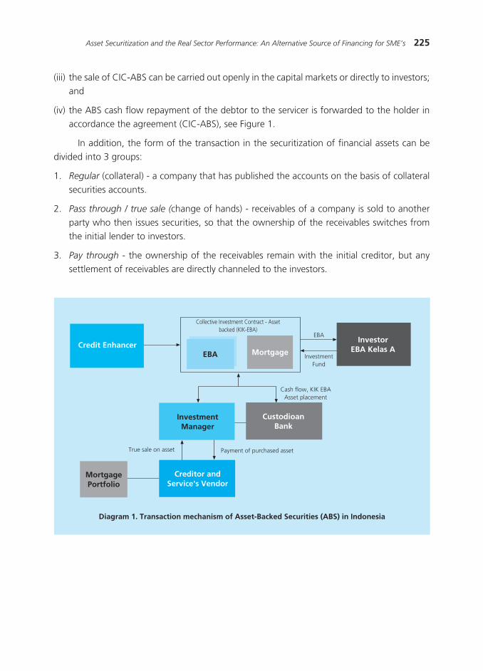
225Asset Securitization and the Real Sector Performance: An Alternative Source of Financing for SME’s
Diagram 1. Transaction mechanism of Asset-Backed Securities (ABS) in Indonesia
(iii) the sale of CIC-ABS can be carried out openly in the capital markets or directly to investors; and
(iv) the ABS cash flow repayment of the debtor to the servicer is forwarded to the holder in accordance the agreement (CIC-ABS), see Figure 1.
In addition, the form of the transaction in the securitization of financial assets can be divided into 3 groups:
1. Regular (collateral) - a company that has published the accounts on the basis of collateral securities accounts.
2. Pass through / true sale (change of hands) - receivables of a company is sold to another party who then issues securities, so that the ownership of the receivables switches from the initial lender to investors.
3. Pay through - the ownership of the receivables remain with the initial creditor, but any settlement of receivables are directly channeled to the investors.
���������������
����������������������������������������� ���������
���
��
�������� ��������������
�� ���������������
������������������������������
�������������
�� ��������������
��������������������������
��������������� ������������
������������������
����������������

226 Bulletin of Monetary, Economics and Banking, Volume 17, Number 2, October 2014
From Table 2, the calculation of interest rates can be obtained as described below:
��������������������������������������� ������������������������������
������������������������������ ����������������������
�� ���������������� �
�� �������� �������� ���������� �����������
�� ���� ������������ ����������������
� � �� � �� �� ��������� ����������������
�� ���������������������� ��������� ��������
� ����
�� ��� ���� ��� ������������������
�� ��� ���� ������ �� ��� ������� ��������������
�� ��������
�� ��� ���� ���������� ��������� �������������� �����
� ������������� ������������
� ���� ��� ��������������������������� ������ �
�� ���� ��� �� ������������������������������ �������
� ������
�� ����� ������������������ �������� �������������
���������������� ��������� �������� �����������
��� ����������� ��������� �����
Research conducted in 2011 showed that the securitization of assets to provide benefits to the relevant parties involved and to the economy. Banks can improve their Capital Adequacy Ratio (CAR) and increase liquidity, which in turn would increase their capacity to lend. Securitization of assets would also increase the money supply (M2) mainly through the process of doubling the money. Loans and purchases of assets by a Special Purpose Vehicle (SPV) has the potential to increase the money supply through increased liquidity so that banks can increase the credit granted.
When viewed from each of the parties involved, the benefits derived from the application of asset securitization is as follows:
Table 2 (below) illustrates the calculation of costs and returns in asset securitization transactions.

227Asset Securitization and the Real Sector Performance: An Alternative Source of Financing for SME’s
���������������������������������� �����
����� �������
�������������������������� ���� � � �������������������������������������� ������������������������������� ����������������������� �������������������������������������� ��������������������������������������������������������
����������� �������������������������������������������� ����������������������������������
������������������������ ��� � ���������������������������������������������������������������� � ������ ���������������������������������������������������������������������� � ���������������������������������������� �������������������������������������������� � �������������������������������������������������������������
������������� � ��������������������������������
� �������������������������������� � �������������� ������������������������������������������
��������������������� ���������������������������������������
Based on the results of a 2011 study, SME asset securitization models are recommended to be applied in Indonesia as a model that has a guarantee. Guarantee given by the Government or external institutions is expected to increase the interest of investors to buy SME-ABS because of the guarantee of investment (safe investment). This is expected to accelerate the development of SME securitization of assets, because it would encourage banks to participate in the development of SME asset securitization.
This mechanism requires the government to provide funds in the event of default of payment by SMEs, as well as forming a guarantors using non-governmental organizations or empowering existing institutions of such guarantora, e.g. ASKRINDO and JAMKRINDO.
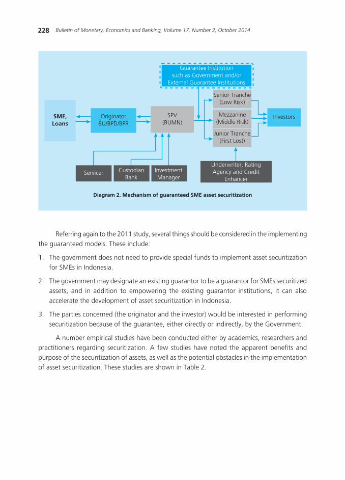
228 Bulletin of Monetary, Economics and Banking, Volume 17, Number 2, October 2014
Diagram 2. Mechanism of guaranteed SME asset securitization
����������������������������������������������
������������������������������
����������������������
����������������������
�������������������������
��������������� �
�������������������
���������
������� �������������
�����������������
������������������������������������
�������
Referring again to the 2011 study, several things should be considered in the implementing the guaranteed models. These include:
1. The government does not need to provide special funds to implement asset securitization for SMEs in Indonesia.
2. The government may designate an existing guarantor to be a guarantor for SMEs securitized assets, and in addition to empowering the existing guarantor institutions, it can also accelerate the development of asset securitization in Indonesia.
3. The parties concerned (the originator and the investor) would be interested in performing securitization because of the guarantee, either directly or indirectly, by the Government.
A number empirical studies have been conducted either by academics, researchers and practitioners regarding securitization. A few studies have noted the apparent benefits and purpose of the securitization of assets, as well as the potential obstacles in the implementation of asset securitization. These studies are shown in Table 2.

229Asset Securitization and the Real Sector Performance: An Alternative Source of Financing for SME’s
������������������������������������ �����������
�� ������ ������������������������
�
�
�
�
�
��������������������� �������������������������������
��������������������������������� �������� ������������������������������������������������������������ �������
������������������������� ������������������������������������������� �������������������������������������������������������� �������������������� ����������������������������������������������������������������������������
������������ �������������� ��������������������������������� ��
���������������������������� �������������������������������������������������������������������������������������������������������������������
����������������������������������� ����������������������������������������������������������� ��������������������������������������������������������� ����������������� �������������������� ��������������� ����������������������������������������������� ���������������� ����������������������������������������������������� ������������������� ��������������������������������� �������� ��������������������������������������������������������������������������������������������������������������������������������������������������� ������������������������������������������������������������������������������������������������� ���������������������������������������������������������������������������������������������� ���������������������������������������������������� �������������������������������� ������� ������������������������������������������������������� �������������� ����������������������������������������������������� ������������������������������������������� ���������������������������������������������������������������������������������������������� ������������������������������������������ �� �������������������������������������������������������������������� ���������������� ��������������������� ������������������������������������������������������������������ ��������������������������������������������������������������������������������������������������� ����� ������������������������������������������������������������������������������������������������������������������������������ ������������������������ ����������
���������������������������������������������������������������������������������������������������������������������������������������������������������������������������������������������� ���������������������������� ���������������������������������������������������������������������������������������������������� ���������������������������������������������������������������������������� ������������������������������������������������������� �������������� ��
����������������� ��������� ����������������������������������������
�������������������������������� �������������������������������������������������������������������� �������������������������������������������������������������������������������������������������������� ������������������� ������������������������������������������������������������������������������������������������������������������������

230 Bulletin of Monetary, Economics and Banking, Volume 17, Number 2, October 2014
The Capital Market Supervisory Agency and Financial Institution (BAPEPAM-LK) together with the Ministry of Finance in 2003 examined the level of stakeholder understanding of asset securitization in Indonesia. The findings from this study showed that most people (57.14% of respondents) quite understood asset-backed securities. Yet only a small percentage who had experience related to the securitization process conducted this abroad, i.e. only the securities rating and legal consultants. Potential investors in the process of asset securitization included companies involved in pension funds, insurance, banking, non-bank financial institutions, and mutual funds, among other large companies. It was argued that ABS could be used as a means of hedging. In the study, major constraints were presented in issuing ABS. Such constraints include:
a. A lack of understanding of the ABS instrument by the issuer and / or potential investors.
b. Disclosure obligations by candidate issuers were feared to lead to a misuse of information.
c. The relevant parties involved considered the existing legislation inadequate (ranging from accounting, taxation, and calculation methods)
d. The need for guidelines governing the accounting for CIC-ABS, such as expectations for granting tax exemption for CIC-ABS.
III. METHODOLGY
3.1. Data and Respondents
The data collection methods in this study used surveys and focus group discussions (FGD). A structured questionnaire was used for the survey and the sample of respondents was selected by purposive sampling. The survey was conducted in Greater Jakarta, Bandung, Yogyakarta, Denpasar, Medan, and Banjarmasin. The sample of respondents consisted of Commercial Banks (CB), Regional Development Banks (RDB), and Rural Banks (RB), all of which were categorized as ‘ABS Issuer’. Pension funds, insurers, and foundations were categorized as an ‘Investor’. SMEs, and the Guarantor Institution are the other categories. A total of 149 respondents were sampled. The following table shows the distribution of the respondent survey by city.
��
����������� �� � �� �� � � �������� � � � � � � ���� ����� � � � � � � ��������� � � � � � � ������� � � � � � � ������������ � � � � � � ������� �� � �� �� �� � ���
�������������������������������� ��������������
��� ��
��� �������� ������� ��� �������� ���������� �����

231Asset Securitization and the Real Sector Performance: An Alternative Source of Financing for SME’s
Respondents (issuers, investor and SMEs) who participated in the survey are noted in Table 5:
�
�
�
�������������������������� ��������
�� ���������������� �������� ����������������������
��������������������������������� ������������������������������������� ������������������������������������������������������������������������������������������������������
����� ���������������������
�������������������������������� ���������� ����������������� �������� ���� �������������������������������������
��������������������������������������������������������
��������������������������������������������������������
�������������
3.2. Data Processing
Surveys in this study used Maximum difference scaling (MaxDiff) technique (see Cohen and Markowitz, 2002). Selection of this method aimed to improve the validity of the data collected, especially data relating to the preferences or the use of this type of investment (asset securitization vs. other types of SME investments). Based on experience, measuring the level of preference or usage with the ranking of data would be difficult for respondents, especially in rating on large amounts of data (5 upwards). By using MaxDiff, the process was straight-forward in which respondents were only asked to choose from a small group of data that was ‘most needed’ and ‘not needed’. The MaxDiff measurement and analysis developed by Jourdan Louviere was used where each alternative had a certain probability to be selected.
Where i is the alternative choice while k is the total of all alternative choices.
Alternative j will be selected only after compared with other alternatives. The alternatives have the greatest value p. The approach taken to obtain the alleged parameter v is the Maximum Likelihood (ML) or with Hierarchical Bayes (HB). For this survey, the parameter estimation approach was based on the HB method. This method, according to Louviere, does not require a high number of samples, in contrast to the ML.

232 Bulletin of Monetary, Economics and Banking, Volume 17, Number 2, October 2014
The advantages of the HB parameter estimation method is in guessing an individual result, where a segment estimate would “add up” data from each individual. This differs from the method in which each segment requires a different estimation process. The analysis results collected using the MaxDiff method was used to obtain conjectures related to demand for ABS investment to attract investors.
This paper also applied SWOT analysis. This analysis can be understood as a system to test an organization’s internal strengths, weaknesses and the external environment opportunities and threats to the organization. SWOT analysis is a method designed for use in the early stages of decisión-making and as a basis for strategic planning of the various situations (Johnson et al., 1989; Bartol et al., 1991).
Gap analysis was also used to examine ABS implementation in Indonesia. Gap analysis examines the differences between the current state and ideal condition, and how to address these differences to improve current state in moving towards the ideal condition/situation. More specifically for this research, gap analysis was used to examine the current situation of the relevant parties involved in asset securitization, including government policies, which were then compared to the expected conditions for the implementation of SME asset securitization.
IV. RESULTS AND ANALYSIS
To recap, the first section of this paper reviewed the dynamics of lending and business development especially SMEs in Indonesia. The actual conditions for lending will be analyzed more in depth based on the survey results and the SWOT and GAP analysis mentioned earlier.
From 2010 - 2012, the realization of increased lending growth among banks was quite encouraging, especially among RDBs. However RBs saw contraction in 2011 due to increasing competition among RBs in lending and the vigorous commercial bank offerings of credit to consumers. The commercial business sector and the manufacturing sector were the sectors most targeted by banks for lending.
Commercial bank (CB) lending increased by approximately 20%, while RDB lending saw a surge in average growth, from 16% in 2010 to 81% in 2011. In contrast, RB lending saw setbacks in growth, from an average of 27% in 2010 to an average of 8% in 2011. This was due to increased competition among RBs in lending.
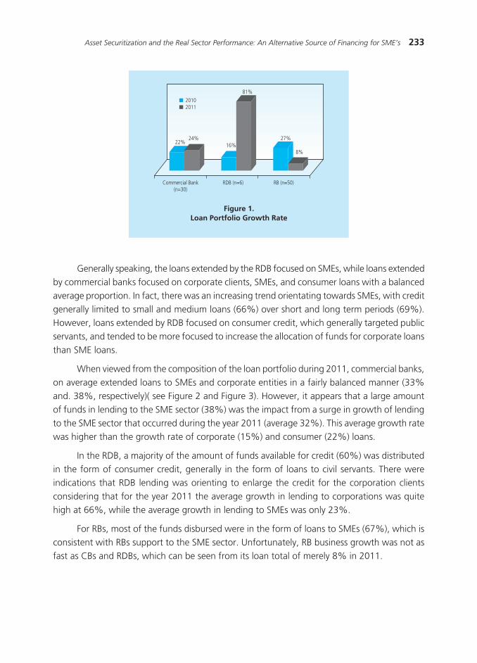
233Asset Securitization and the Real Sector Performance: An Alternative Source of Financing for SME’s
Generally speaking, the loans extended by the RDB focused on SMEs, while loans extended by commercial banks focused on corporate clients, SMEs, and consumer loans with a balanced average proportion. In fact, there was an increasing trend orientating towards SMEs, with credit generally limited to small and medium loans (66%) over short and long term periods (69%). However, loans extended by RDB focused on consumer credit, which generally targeted public servants, and tended to be more focused to increase the allocation of funds for corporate loans than SME loans.
When viewed from the composition of the loan portfolio during 2011, commercial banks, on average extended loans to SMEs and corporate entities in a fairly balanced manner (33% and. 38%, respectively)( see Figure 2 and Figure 3). However, it appears that a large amount of funds in lending to the SME sector (38%) was the impact from a surge in growth of lending to the SME sector that occurred during the year 2011 (average 32%). This average growth rate was higher than the growth rate of corporate (15%) and consumer (22%) loans.
In the RDB, a majority of the amount of funds available for credit (60%) was distributed in the form of consumer credit, generally in the form of loans to civil servants. There were indications that RDB lending was orienting to enlarge the credit for the corporation clients considering that for the year 2011 the average growth in lending to corporations was quite high at 66%, while the average growth in lending to SMEs was only 23%.
For RBs, most of the funds disbursed were in the form of loans to SMEs (67%), which is consistent with RBs support to the SME sector. Unfortunately, RB business growth was not as fast as CBs and RDBs, which can be seen from its loan total of merely 8% in 2011.
Figure 1.Loan Portfolio Growth Rate
Commercial Bank(n=30)
RDB (n=6)
22%24%
16%
20102011
81%
27%
8%
RB (n=50)

234 Bulletin of Monetary, Economics and Banking, Volume 17, Number 2, October 2014
Although SME were predominantly financed by the banks, the banks generally had difficulty in mentioning the type of businesses they financed. By triangulation of the date, it was found that a large portion of bank lending to SMEs was in retail trade enterprises, with the proportion varying fro 15% to 80% of the total amount of credit. After the retail trade sector, the SMEs sectors that received the most loans from banks were those engaged in the processing industry (75%), such as garment, furniture and food processing with the proportion of loans disbursed between 9% to 40%. The third largest was agriculture and plantations (51%) with a proportion of loans disbursed between 6% to 35%.
Figure 2.Composition of Loans Disbursed
Figure 3.Cross-scale User Credit Growth
31%
20% 20% 60%
33% 38% 28%
67%2%BPR (n=50)
BPD (n=6)
Bank Umum (n=30)
SME LoansKredit Korporasi Consumer Loans
Corporate LoansCorporate LoansCorporate Loans
Commercial Bank (n=30)
15%
32%
22%
66%
23%17% 17%
5% 7%
RDB (n=6) RB (n=50)
����� ���������������������� ��������������������������������� �������������������������������������� ����������� ����������������������������������������� �������� �������������� ���������������� ��� ������������������������������������������ �������� �������������������������������������������������� ����������� ���
�������������������������� ����������������
��������������� �����������
Examination of the credit plan and its realization showed that the respondents were not able to meet their targets. It is assumed that the main obstacle was intense competition between banks (59%) to the capture eligible customers as the size of the customer base

235Asset Securitization and the Real Sector Performance: An Alternative Source of Financing for SME’s
remained relatively unchanged with only minor variations from year to year. As for RBs, the competition was more difficult because the interest rate charged by RBs was higher than the rate set by conventional banks. Also, the business conditions of SMEs might have been seen as less favorable due to its low purchasing power since a) SMEs are often businesses of low- to middle-income communities, b) government protection against SME businesses tends to be minimal, and c) it is difficult for SMEs to expand their business.
4.1. Issuers
The survey results showed that issuers’ understanding of securitization varied. Commercial banks and regional development banks had a higher level of awareness than rural banks. Of the rural banks, 25% had never heard the term securitization. Overall understanding of securitization among the issuers was inadequate.
Although the concept of SME-ABS was considered quite attractive by the issuers, there were several factors that influenced interest for issuers to offer SME loans in the form low SME-ABS. For issuers, limitations in lending to SMEs was not because of a shortage of funds, although in the last few years commercial banks and RDBs typically experience excess liquidity. Barriers to increase lending to SMEs were more due to highly competitive conditions in a small less developed SME market. Despite a relatively stagnant market niche, SMEs were still bankable. Moreover, banks were likely to implement a vigorous acquisition strategy that included take-over offers of credit with low interest.
Furthermore, lending to SMEs required a labor force large enough and with adequate support technology. SME loans are big volume and low value which required adequate assistance to SME customers so that the level of NPLs can be maintained. These conditions led to a perception of SME-ABS, that although considered quite attractive, the interest to sell SME loans in the form SME-ABS was low.
The biggest concern for the issuer in implementing a SME-ABS is the risk of failing in the management. Lending to SMEs should be accompanied by good observation and coaching, such as regular visits or consultations. When the SME receivables are sold, then the focus of attention would shift to address new customers who are funded from the sale of these assets. So there was concern that they will not be able to guarantee or maintain the performance of the receivables sold.
Concerns were related to the unpreparedness of the human resources that have difficulties in handling the administration of a special nature. To be able to increase lending to SMEs a labor force large enough and adequate assistive technologies are needed since lending to SMEs are high volume and low value.

236 Bulletin of Monetary, Economics and Banking, Volume 17, Number 2, October 2014
Another concern was the risk that SMEs make early payment while investors have chosen the payment system of fixed cash flows (pay through), especially considering that the practice of take-over SME loans in the banking sector is quite high. And in this regard it was feared that ultimately it would be an additional burden of having to replace the administrative work of SME receivables that have been securitized with other receivables.
The problem of legal uncertainty / rules were also a concern for others, especially with the pe-rating criteria as well as the performance of the agencies ‘pe-rating’ itself. Therefore, the issuer generally assumed that the securitization of SMEs receivables can not be done as easily as the securitization of housing loans. There is a growing niche market for housing loans commensurate with population growth, while the actual SME credit niche market is growing very slowly (due to the slow growth of bankable SMEs). Therefore, when the securitization is to be done, the majority of respondents (59%) were only willing to release the receivables of poor / very poor quality. Even for those banks willing to release the receivables of SMEs with good / very good quality, 33% of them stated that they would feel real disappointment in releasing these receivables for securitization in considering that the profits are not commensurate with the efforts that have been made and the risks involved in SME lending. Thus, the majority of respondents (65%) refused to buy the ABS. The whole concern is exacerbated by the lack of a clear understanding of SME-ABS due to inadequate education and awareness raising.
Indeed, the main attraction of the securitization concept of the SME-ABS product is (i) it can be used as an instrument to control credit risk, (ii) to address the shortage of funding,
������������������������������������������������� ������������������������������ ������������������������������������������������������ ������������������ ��������������������� �������������������������������������������������������������������� ���������������������� ������������������������������� ����������������������������������������������������������������������������������������������������������������������������������� ��������� ������������������������������������������������������������������ ���������������� ����������������������������������������� ���������������������������������������������������������������������������������������� ������� ���������������������������������� � ����������
���������������������������� �������� ���������������������
���
���
���
���
��
������
��
��
���
���
��
���
������
��
���
��
���
���
��
������
��
���
��
���
���
��
������
��
������� ���������������
���� �� �
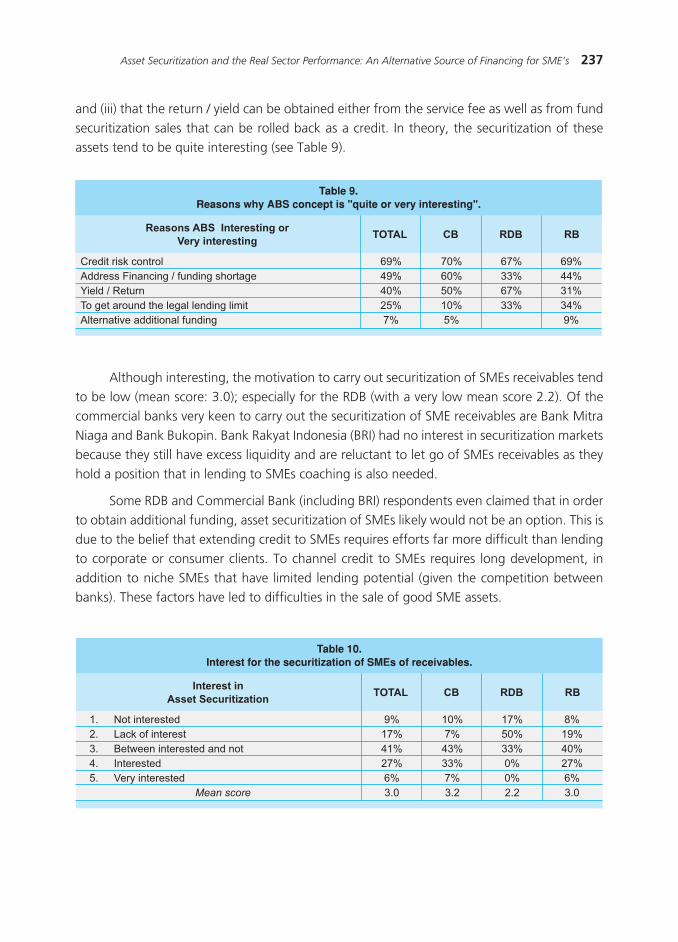
237Asset Securitization and the Real Sector Performance: An Alternative Source of Financing for SME’s
and (iii) that the return / yield can be obtained either from the service fee as well as from fund securitization sales that can be rolled back as a credit. In theory, the securitization of these assets tend to be quite interesting (see Table 9).
������������������� ��� ��� ��� ��� ������������������������������� ��� ��� ��� ���������������� ��� ��� ��� ������������������������������������� ��� ��� ��� ��� ���������������������������� �� �� � ��
������������������������ �� �����������������������������
�������������������������������������������
� ��� ��� ���
Although interesting, the motivation to carry out securitization of SMEs receivables tend to be low (mean score: 3.0); especially for the RDB (with a very low mean score 2.2). Of the commercial banks very keen to carry out the securitization of SME receivables are Bank Mitra Niaga and Bank Bukopin. Bank Rakyat Indonesia (BRI) had no interest in securitization markets because they still have excess liquidity and are reluctant to let go of SMEs receivables as they hold a position that in lending to SMEs coaching is also needed.
Some RDB and Commercial Bank (including BRI) respondents even claimed that in order to obtain additional funding, asset securitization of SMEs likely would not be an option. This is due to the belief that extending credit to SMEs requires efforts far more difficult than lending to corporate or consumer clients. To channel credit to SMEs requires long development, in addition to niche SMEs that have limited lending potential (given the competition between banks). These factors have led to difficulties in the sale of good SME assets.
�� �������������� �� ��� ��� ���� ������������� ��� �� ��� ����� �������������������������� ��� ��� ��� ����� ���������� ��� ��� �� ����� ��������������� �� �� �� ��
���������� ��� ��� ��� ���
����������������������������� ��������������������������������
�������������������������������
����� �� ��

238 Bulletin of Monetary, Economics and Banking, Volume 17, Number 2, October 2014
For the implementation of SME-ABS, 21% of banks stated that asset securitization is feasible to run immediately within a period of one year to the next. Most RBs (75%) felt this way, and they in general had very inadequate knowledge about securitization of SME-ABS. Overall, 41% of respondents thought it was only feasible to carry out for 2-5 years, while 23% felt it was feasible after more than 5 years, and 16% gave no time of certainty.
4.2. Investor
There are various forms of investment made by the investor. Each investor generally allocates the investment in 2 to 4 forms. The allocation of investment funds is generally done at a maximum of 25%. The most commonly used investment are bonds (60% of respondents), Bank Indonesia Certificates (BIC) (52% of respondents, the majority commercial banks), and deposits (52% of respondents). In all three forms of investments, respondents invested more than 75% their investment funds.
In general, BIC seems to be the most preferred form of investment - especially by commercial banks, since 20% of the total of 25 respondents invested more than 75% of funds, while 12% of respondents invested between 51% - 75% of investment funds that are owned.
Assuming that there are nine (9) kinds of investments that can be made and the investor may only select one (1) type of investment, the share of preference for BIC is the highest (i.e. 21%, in other words, the average propensity to invest funds in BIC products amounted to 21% of the total funds held); while SME-ABS ranked second (19%), on condition of an 11% minimum interest rate, which is higher than the share of interest bonds or deposits that have always been a form of investment other than BIC. The preference for SME-ABS at 19% reinforces the findings that the amount of money available to invest in the SME-ABS product is equivalent to 10% - 15% of the total investment fund (Figure 6).
Figure 4.Preference of Funds Placement by Banks
2%Valas
Reksadana
Emas
Saham
Sukuk
Obligasi
Deposito
EBA
SBI
4%
4%
9%
11%
14%
n = 25
16%
19%
21%
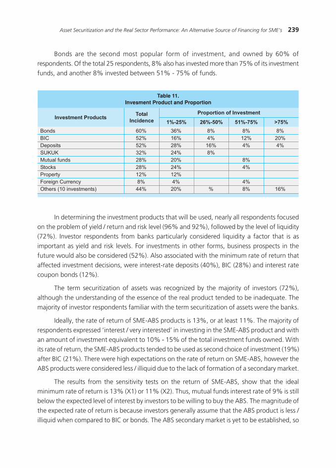
239Asset Securitization and the Real Sector Performance: An Alternative Source of Financing for SME’s
Bonds are the second most popular form of investment, and owned by 60% of respondents. Of the total 25 respondents, 8% also has invested more than 75% of its investment funds, and another 8% invested between 51% - 75% of funds.
In determining the investment products that will be used, nearly all respondents focused on the problem of yield / return and risk level (96% and 92%), followed by the level of liquidity (72%). Investor respondents from banks particularly considered liquidity a factor that is as important as yield and risk levels. For investments in other forms, business prospects in the future would also be considered (52%). Also associated with the minimum rate of return that affected investment decisions, were interest-rate deposits (40%), BIC (28%) and interest rate coupon bonds (12%).
The term securitization of assets was recognized by the majority of investors (72%), although the understanding of the essence of the real product tended to be inadequate. The majority of investor respondents familiar with the term securitization of assets were the banks.
Ideally, the rate of return of SME-ABS products is 13%, or at least 11%. The majority of respondents expressed ‘interest / very interested’ in investing in the SME-ABS product and with an amount of investment equivalent to 10% - 15% of the total investment funds owned. With its rate of return, the SME-ABS products tended to be used as second choice of investment (19%) after BIC (21%). There were high expectations on the rate of return on SME-ABS, however the ABS products were considered less / illiquid due to the lack of formation of a secondary market.
The results from the sensitivity tests on the return of SME-ABS, show that the ideal minimum rate of return is 13% (X1) or 11% (X2). Thus, mutual funds interest rate of 9% is still below the expected level of interest by investors to be willing to buy the ABS. The magnitude of the expected rate of return is because investors generally assume that the ABS product is less / illiquid when compared to BIC or bonds. The ABS secondary market is yet to be established, so
����� ��� ��� �� �� ����� ��� ��� �� ��� ����� ����� ��� ��� ��� �� ���� ��� ��� �� ������������� ��� ��� � ������� ��� ��� � ����� ���� ��� ��� � ����������������� �� �� � �� ��������������������� ��� ��� � �� ���
����������������������� ����������������
������������������������
��������� ��� ����� ���� ���
������������������������

240 Bulletin of Monetary, Economics and Banking, Volume 17, Number 2, October 2014
it is feared it will be difficult to resell the ABS. Investors need to invest in a high compensation EBA with a low level of liquidity.
Preferable SME-ABS issuers are commercial banks, i.e. CB state-owned enterprises (92%), although only 68% of respondents were willing to invest in SME-ABS products issued by CB national private banks.
��������������������� � �������������������������������� ���������������������������������� ������ � ��� ��
�������������������������� ��
���������� ������������
Three main criteria expected of a bank to became an ABS issuer include, i) the bank must have a good reputation in the eyes of the public or a bank that is actually healthy (56%), ii) has assets large enough (28%), and iii) experienced in the distribution SME loans (28%). The main business sector with a demand for ABS products is the trade and processing industry sectors. The preferred guarantor is a guarantor institution owned by the Government.
����� ��������������������� �������������������������������� ��������� ����������� ��������������� ��������� ���
����������������������� �������� ���������� �����
��������������� ������������
Most investors believe that when implemented within 3-4 years to come, SME-ABS will be able to run well. Based on the questions concerning the plan of ABS implementation, most respondents investors (56%) doubt that the securitization of SMEs receivables can be run properly implemented within 1-2 years, even 8% stated unequivocally that it cannot be implemented in 1- 2 years’ time. Only 36% were convinced that the securitization of receivables of SMEs could work well if implemented within 1-2 years.

241Asset Securitization and the Real Sector Performance: An Alternative Source of Financing for SME’s
It is interesting to observe that the respondents who doubted or firmly reject the implementation of SME-ABS were few, as it turns out the vast majority (75%) felt confident that when implemented within 3-4 years to come, it could run well. This reinforces the idea that in order for the SME-ABS interest, there should be an established secondary market developed.
Only 24% of respondents (6 of the total 25 respondents) felt very pessimistic about the successful implementation of SME-ABS, arguing that preparing the market and its supporting institutions would not be easy and requires hard work and a long time, at least 10 years. The important factors to be considered in the implementation of SME-ABS are noted in Table 16.
���������������������������������������������������������������� ����������������������� ������������������������������ ����������� ��������������������� �������������������������������������������� ����������������������������������� ������������ ���������������������������������������� ������������������������������� ��� ������������������������������������������ �
���������������������������� ��� ���������
������� �����������������������
Most investors (56%) believe that the SME-ABS will be able to run properly if it is implemented in the medium term, i.e. 3-4 years to come. While most other investors (24%) are pessimistic towards the successful implementation of SME-ABS, by reason of preparing the market as well as supporting institutions that will be difficult and require hard work over a very long time. There are several important factors that must be considered when implementing SME-ABS, namely: (i) clear rules about the structure of the transaction and the parties involved in the transaction EBA (52%); (ii) government support through legislation (20%), (iii) the execution of a clear guarantee that is fully protected by law (16%); (iv) the existence of guarantor institutions that can be trusted (16%); (v) the ratification of proper rules (12%); fulfillment of legal regulations (8%), and (vi) the support of regulators such as BI and BAPEPAM LK.
4.3. Insurance / Insurance Agency
Guarantor institutions or insurance companies that provide guarantees on loans still do not seem to be sufficiently developed in Indonesia. This is evident from the difficulties faced to get target respondents from segments of guarantor institutions and credit company guarantee institutions, most of which are owned by the central government or local governments. But even so, there are indications of business growth of guarantor agencies, as seen from the growth
242 Bulletin of Monetary, Economics and Banking, Volume 17, Number 2, October 2014
in the number of permanent employees absorbed in this industry to accompany the reduction in the number of contract employees.
The government gave attention to guarantor institution belonging to the central and local governments with a capital injection in 2011 between 5% -35%. Credit guarantors for SMEs are not a new thing for company guarantor institutions. In general, SME loans are considered more risky than corperate credit and mortgages. This can be seen from the higher fee charged by the guarantor institution and lower underwriting value. The level of risk and business prospects in the foreseeable future is the main thing to be considered in giving a guarantee for an investment product.
For a guarantee / insurance on corporate credit, the proportion recorded for a guarantee on corporate credit products ranged from 5% - 87% of the total business value. Loading costs were generally less than 4% and ranged from 1.5% - 3.8%. The guarantee covers between 75% - 100% of the value of the credit. While for other products including SME loans, the proportion of product guarantee loans ranged from 5% - 100% of the overall value of the business. The loading charge (fee) is the same which ranged from 1.5% - 3.8%, and the guarantee covered between 70% - 100% of the value of the credit.
Most institutional guarantor (6 of 8 respondents), expressed ‘interest / very interested’ to become a guarantor institution for SME-ABS products. Those less interested were ACA Insurance and Askrindo, because they thought SME NPLs were quite high, and they were not interested in any further information about the SME-ABS product with all the potential risks and benefits.
In offering insurance, there is general practice of reinsurance or company-backed by a guarantor institution / other insurance. Examples of companies that are commonly used for this purpose are Marein and ReINDO. In running the daily business and in expanding their reach, the main obstacles is the lack of capital and limited human resources, both for the purposes of marketing their products and expertise in the management of insurance.
SME-ABS are less known by most company guarantor institutions, and SME-ABS products are considered as an investment product with moderate to high level of risk. This assessment is based on the assumption that SMEs generally have more traditional business management with irregular management practices of a limited track record, and located in places susceptible to fire. There is also the presumption that SME NPL is high.
Nonetheless, most guarantor institutions were ‘interested / very interested’ to become a guarantor for SME-ABS products, in particular for SME-ABS issued / sold to the trade sector by the state-owned commercial banks with charges (fee) ranging from 2.5% - 5%. The next attractive sector was the the financial sector, real estate and business services, construction, manufacturing and tourism, and with charges greater than 1% with an average coverage guarantee to a maskimal of 73.8%.
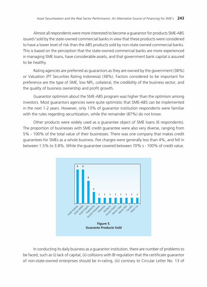
243Asset Securitization and the Real Sector Performance: An Alternative Source of Financing for SME’s
Almost all respondents were more interested to become a guarantor for products SME-ABS issued / sold by the state-owned commercial banks in view that these products were considered to have a lower level of risk than the ABS products sold by non-state owned commercial banks. This is based on the perception that the state-owned commercial banks are more experienced in managing SME loans, have considerable assets, and that government bank capital is assured to be healthy.
Rating agencies are preferred as guarantors as they are owned by the government (38%) or Valuation (PT Securities Rating Indonesia) (38%). Factors considered to be important for preference are the type of SME, low NPL, collateral, the credibility of the business sector, and the quality of business ownership and profit growth.
Guarantor optimism about the SME-ABS program was higher than the optimism among investors. Most guarantors agencies were quite optimistic that SME-ABS can be implemented in the next 1-2 years. However, only 13% of guarantor institution respondents were familiar with the rules regarding securitization, while the remainder (87%) do not know.
Other products were widely used as a guarantee object of SME loans (6 respondents). The proportion of businesses with SME credit guarantee were also very diverse, ranging from 5% - 100% of the total value of their businesses. There was one company that makes credit guarantees for SMEs as a whole business. Fee charges were generally less than 4%, and fell in between 1.5% to 3.8%. While the guarantee covered between 70% s - 100% of credit value.
Figure 5.Guarante Products Sold
Kredit K
opera
si
Kredit U
MKM
Kredit P
ropert
i
Engin
eerin
g
Asuran
si Kary
awan
Perba
nkan
Multigu
na
Asuran
si Exp
ort
Marine
Cargo
Marine
HUU
Casualit
y
Motor C
ar
6 6
4
2
1 1 1 1 1 1 1 1
In conducting its daily business as a guarantor institution, there are number of problems to be faced, such as (i) lack of capital, (ii) collisions with BI regulation that the certificate guarantor of non-state-owned enterprises should be in-rating, (iii) contrary to Circular Letter No. 13 of

244 Bulletin of Monetary, Economics and Banking, Volume 17, Number 2, October 2014
2011 regarding the ATM Care in circular: ATM Care point for the Bank is 20% while the rating is adjusted for private sector; (iv) the difficulty to convince the market about the importance of the guarantee, (v) lack of human resources in each area, (vi) lack of investment options from the regulator; (vii) the banks often include SMEs that are not qualified which sometimes runs a risk; (viii) enterprises have not been listed officially as a partner guarantor institution, so that the bank preference goes to SOEs; and (ix) risks of global trade, and competition between insurance agencies.
Meanwhile, to expand the range, the biggest obstacle is the perceived problem of capital as well as limited human resources, both for the purposes of marketing products and expertise in the management of insurance. In providing guarantee for an investment product, the most important consideration is the level of risk and future business prospects.
SME sectors with guarantors willing to guarantee ABS products, are the trade sector, followed by the financial sector, real estate and business services, construction, manufacturing and tourism with an average coverage of the guarantee willing to be borne at 73.8%. However, the desired fee was greater than 1%. With a fee of 1%, only part of the institution was willing to be a guarantor for SME-ABS products. This is understandable considering that the fee received is between 1.5% - 5%. The survey also showed that in general a guarantor for SME-ABS products expect a fee between 2.5% - 5%.
4.4. SMEs
SME business development has been quite good. In 2010 and 2011, all SMEs had fairly stable business turnover, which tended to increase in 2012. Over the years, some had increased profits. But even so, still quite a number of SMEs (with a business turnover of at least Rp. 300 million / year) did not have legal status and only the status of individual property (30%). Many operated only by relying on the Business License from the village. In fact, most SMEs (57%) still used manual financial records for financial management.
Loans obtained from the Bank were generally used for working capital and investment. But some SMEs were using it for the welfare of employees (3%), generally with medium credit period (1 s / d 3 years). BRI was of the most accessible banks (27%), followed by Bank Mandiri (17%) and rural banks (13%), with a common interest rate ranging between 12% - 14%. The SMEs generally assumed that a reasonable interest rate is 10% - 12%, or 2% lower than the prevailing interest rate.
Most SMEs (83%) said they never have problems meeting re-payment obligations on loans obtained from the Bank. Only 17% (or 5 SMEs) encountered some problems, which was generally caused by delays in payments made by the customer, the decreased number of customers, uncertain weather that inhibits the production processes, interest deemed too burdensome, stoppage of activity due to earthquake (as occurred in Jogjakarta). Banks turned
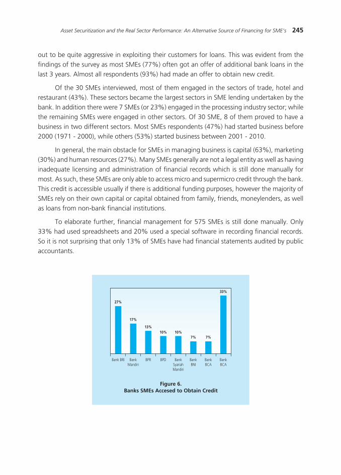
245Asset Securitization and the Real Sector Performance: An Alternative Source of Financing for SME’s
out to be quite aggressive in exploiting their customers for loans. This was evident from the findings of the survey as most SMEs (77%) often got an offer of additional bank loans in the last 3 years. Almost all respondents (93%) had made an offer to obtain new credit.
Of the 30 SMEs interviewed, most of them engaged in the sectors of trade, hotel and restaurant (43%). These sectors became the largest sectors in SME lending undertaken by the bank. In addition there were 7 SMEs (or 23%) engaged in the processing industry sector; while the remaining SMEs were engaged in other sectors. Of 30 SME, 8 of them proved to have a business in two different sectors. Most SMEs respondents (47%) had started business before 2000 (1971 - 2000), while others (53%) started business between 2001 - 2010.
In general, the main obstacle for SMEs in managing business is capital (63%), marketing (30%) and human resources (27%). Many SMEs generally are not a legal entity as well as having inadequate licensing and administration of financial records which is still done manually for most. As such, these SMEs are only able to access micro and supermicro credit through the bank. This credit is accessible usually if there is additional funding purposes, however the majority of SMEs rely on their own capital or capital obtained from family, friends, moneylenders, as well as loans from non-bank financial institutions.
To elaborate further, financial management for 575 SMEs is still done manually. Only 33% had used spreadsheets and 20% used a special software in recording financial records. So it is not surprising that only 13% of SMEs have had financial statements audited by public accountants.
Figure 6.Banks SMEs Accesed to Obtain Credit
27%
17%
13%10% 10%
7% 7%
33%
Bank BRI BankMandiri
BPR BPD BankSyariahMandiri
BankBNI
BankBCA
BankBCA
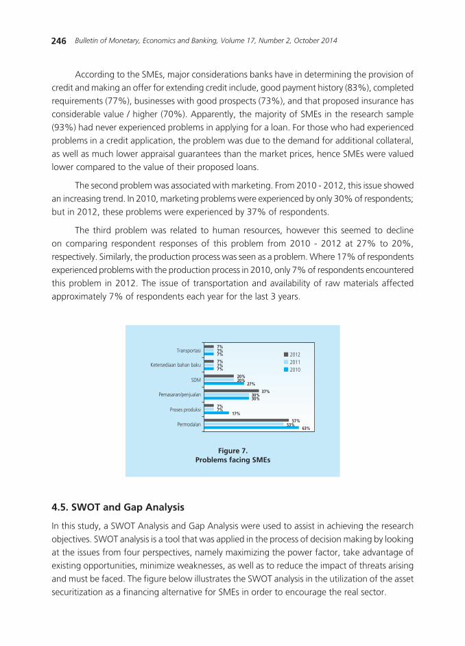
246 Bulletin of Monetary, Economics and Banking, Volume 17, Number 2, October 2014
According to the SMEs, major considerations banks have in determining the provision of credit and making an offer for extending credit include, good payment history (83%), completed requirements (77%), businesses with good prospects (73%), and that proposed insurance has considerable value / higher (70%). Apparently, the majority of SMEs in the research sample (93%) had never experienced problems in applying for a loan. For those who had experienced problems in a credit application, the problem was due to the demand for additional collateral, as well as much lower appraisal guarantees than the market prices, hence SMEs were valued lower compared to the value of their proposed loans.
The second problem was associated with marketing. From 2010 - 2012, this issue showed an increasing trend. In 2010, marketing problems were experienced by only 30% of respondents; but in 2012, these problems were experienced by 37% of respondents.
The third problem was related to human resources, however this seemed to decline on comparing respondent responses of this problem from 2010 - 2012 at 27% to 20%, respectively. Similarly, the production process was seen as a problem. Where 17% of respondents experienced problems with the production process in 2010, only 7% of respondents encountered this problem in 2012. The issue of transportation and availability of raw materials affected approximately 7% of respondents each year for the last 3 years.
Figure 7.Problems facing SMEs
Transportasi
SDM
Permodalan
Proses produksi
Pemasaran/penjualan
Ketersediaan bahan baku
7%7%7%
7%7%7%
7%7%
17%
57%53%
63%
20%20%
27%
37%30%30%
201220112010
4.5. SWOT and Gap Analysis
In this study, a SWOT Analysis and Gap Analysis were used to assist in achieving the research objectives. SWOT analysis is a tool that was applied in the process of decision making by looking at the issues from four perspectives, namely maximizing the power factor, take advantage of existing opportunities, minimize weaknesses, as well as to reduce the impact of threats arising and must be faced. The figure below illustrates the SWOT analysis in the utilization of the asset securitization as a financing alternative for SMEs in order to encourage the real sector.

247Asset Securitization and the Real Sector Performance: An Alternative Source of Financing for SME’s
Figure 8.SWOT Analysis of ABS in Indonesia
Gap analysis, according to businessdictionary.com3, as applied to businesses is a technique to “determine what steps are need to be taken in order to move from its current state to its desired, future state. It is also called need-gap analysis, needs analysis, and needs assessment.” For this research, gap analysis was used to examine the current situation of the relevant parties involved in the securitization of assets, including the policies of the government, which was then compared to the expected conditions for SME asset securitization to idenitify gaps to be filled or addressed. Figure 9 shows the gap analysis approach for SME-ABS in Indonesia.
������������
����������������������������������������� ������������������������������������������������������������������������������������������������������������ ����������������������������������������� ������������������������ ����������������������������������
�������������������������� ���������������������������������������������������������� ������������������������������������������������������������������������������������������ ����������������������������������� ���������������������������������������������������������
��������������������������������������������������������������������������������������������������������������������������� �����������������������������������������������������������������������������������������������������������������
��������������������������������������������������������������������������������������������������������������������������������������������������������������� ������������������������������������������������������������ ������������������������������������������������������������������
��������
�������
������
�����
�������
�����
3 http://www.businessdictionary.com/definition/gap-analysis.html

248 Bulletin of Monetary, Economics and Banking, Volume 17, Number 2, October 2014
Figure 9.Implementation SME-ABS Gap Analysis in Indonesia
From the Figure 9, it appears that in order to close the gaps between the current state and ideal state, there are five things that must be done SME-ABS to be more effectively implemented in Indonesia:
1. As the understanding of SME-ABS is relatively low amongst the relevant parties, it is necessary to increase the understanding of SME-ABS mechanisms and processes through improved the education and dissemination of information to the relevant parties, namely: issuer, investor, and the guarantor institution.
2. There is a need to strengthen the capacity of SMEs which can be done through the support by technical ministries and agencies for effective SME management and good corporate governance (GCG).
3. The provision of supporting regulations followed by its socialization would assist in the implementation of SME asset securitization.
4. There is a need to provide incentives to banks (issuers) for implementing SME asset securitization as the banks have not been keen to securitize SME assets due to the high liquidity of banks.
5. Strengthen and improve the quality of human resources in the banking management of SME loans and credit asset securitization for more effective SME asset securitization.
���������������������������� ������������ ������
�������������������������������������������� �����������������������������������
���������������������������������������������������������������������������������
�������������������������������������������������������������������������������������
����������������������������������������������������������������������������������������
�����������������������������������������������������������������������������
������������������������������������������������ �����������������������������������������������������������
������������������������������������������������������������������������������������������������������������������������������������
��������������������������������������������������������������������������������������������
���������������������������������������������������������������������������������������
�������������������������������������������������� ����������������������������������������������������������������
������������������������������������
�����������������������������������������������������������������������������������������
����������������������������������������������������������������������������������������
����������������������������������������������������������������������������������
249Asset Securitization and the Real Sector Performance: An Alternative Source of Financing for SME’s
V. CONCLUSIONS
The research outlined in this paper involved an array of respondents over a wide scope with focus on the parties involved in securitization as a financing alternative for SMEs. The study concluded that based on the results of surveys and focus group discussions, the implementation of asset securitization as an alternative financing for the real sector and SMEs is not likely to occur in the near future.
Some of the reasons behind this conclusion include among others;
(i) An understanding of the asset securitization businesses of SMEs in Indonesia is not maximized;
(ii) Most of the banks are still not interested in becoming an issuer (original creditor) because a. Liquidity would be in excess, the LDR would still be low;b. There is relative difficulty of finding new SMEs customers;c. The general lack of information and dissemination about the concept of SME asset
securitization; andd. Most banks tend to want to be an investor rather than be an issuer;
(iii) A strong legal basis regarding the preparation of SME asset securitization is still needed, in addition to the need for further integration with provisions concerning CIC-ABS that already exist today;
(iv) The need for incentives for banks when acting as an issuers, such as benefits/reward in taking on risk-weighted assets;
(v) SME asset securitization schemes should be supported by a rating agency in charge of rating SMEs;
(vi) Implementing the model for SME-ABS in the context of Indonesia requires strengthen coordination with relevant agencies; and
(vii) Needed improvements / strengthening of SMEs in terms of management to improve overall performance for good corporate governance.

250 Bulletin of Monetary, Economics and Banking, Volume 17, Number 2, October 2014
references
Bartol, K. M. dan Martin, D. C. 1991, Management, international edition, McGraw-Hill, New York.
Cohen, Steven H. and Paul Markowitz (2002) “Renewing market segmentation: Some new tools to correct old problems.” ESOMAR 2002 Congress Proceedings, 595-612, ESOMAR: Amsterdam, The Netherlands.
Tim Studi Perdagangan Efek Beragun Aset, 2003, Studi tentang Perdagangan Efek Beragun Efek, Departemen Keuangan RI dan Badan Pengawas Pasar Modal, tidak dipublikasikan.
Gan, Yingjin Hila dan Christopher Mayer, 2006, Agency Conflict, Asset Substitution, and Securitization, National Bureau of Economic Research, Cambridge.
Johnson, G., Scholes, K., & Sexty, R. W. (1989). Exploring strategic management. Scarborough, Ontario: Prentice Hall.
Joseph Norton J, et.al., (1993), International Finance in the 1990s. USA: Blackwell Publisher.
Kimborough, Robert T., (1974), Summary of American Law. Lederman Jass 1996, The Hand Book of Asset Backed Securities. Cleveland Ohio., pada Syafaruddin Harahap (2010), Tinjauan Yuridis Kontrak Investasi Kolektif Efek Beragun Aset di Bank BTN, Tesis, Program Studi Magister Kenotariatan, Program Pascasarjana Universitas Diponegoro.

251Determinant of Non Performing Loan: The Case of Islamic Bank In Indonesia
DETERMINANT OF NON PERFORMING LOAN: THE CASE OF ISLAMIC BANK IN INDONESIA
Irman Firmansyah1
This paper analyzes the non-performing loan and its determinant. Using the monthly data of
Islamic banks during 2010-2012, this paper found that size and efficiency of the banks do not affect the
non-performing loan. On the other hand, GDP and inflation negatively affect the non-performing loan,
while the liquidity of the bank positively affects the non-performing loan. The liquidity of also does not
mediate the relationship between the size of the bank, their efficiency, the GDP and the inflation to the
non-performing loan.
Abstract
Keywords: non-performing loan, liquidity, bank size, efficiency, sobel test, Islamic bank.
JEL Classification: C12, G21
1 Lecturer at Department of Economic University of Siliwangi Tasikmalaya, and a consultant at Smart Consulting, email: [email protected].

252 Bulletin of Monetary, Economics and Banking, Volume 17, Number 2, October 2014
I. INTRODUCTION
Banks are important financial institutions affecting the both micro and macro economies. It functions as financial intermediaries between the parties with surplus funds and the parties that need funds or face deficits. In running its business as a financial institution that sells trust and services, each bank attempts to attract as many new customers as possible, increase their revenues, and increase its lending and services (Simorangkir, 2004). According to the Banking
Act No. 10 of 1998, the types of banks in Indonesia consists of commercial banks and rural credit banks (RCB). RCB Islamic banking is represented by the Syariah Rural Credit Banks (SRCBs).
Most banks in Indonesia still rely on credit as a main income of finance to its operations. According to Siamat (2005), one of the reasons the bank business is concentrated on lending is the nature of the business of banks as an intermediary between surplus units to deficit units, and the main source of bank revenue is from the public, so morally an argument can be made that banks should channel back funds to the community in the form of credit. Like other developing countries, bank lending is still a main source for financing business in Indonesia, and it is expected to drive economic growth. Lending is the primary activity of most banks for making a profit, but the greatest risk to the bank is also derived from the provision of credit. Therefore, the provision of credit must be accompanied by rigorous risk management (InfoBankNews.com 2007 in Pratt, 2010).
At banks that operate according to Islamic principles such as SRCBs, the term credit is not used but replaced with the term ‘financing’ as it carries different principles. Unlike credit, financing has more priority elements in the form of agreement and transparency so that the values of Islam are maintained. In general, much of the financing provided to the public is classified as unhealthy category, meaning such financing is of poor quality or problematic. Such unhealthy financing is called Non Performing Finance (NPF) which is prevalent in Islamic and non-Islamic banking. Problems of NPF that go beyond limits unchecked or unresolved, will cause serious problems that will interfere with the profitability of Islamic banks and lead to the cessation of operations, particularly as Islamic banks have small assets compared to the other banking institutions. It is therefore necessary to identify the factors that lead to financing problems in early efforts to address or avoid the situation of NPF, especially for the SRCBs in Indonesia.
Some research about the factors that influence or cause financing problems, both internal and external factors, has been carried out as noted in the following:
From the internal aspect, Adisaputra (2012) found that a positive Operating Expense to
Operating Income (OEOI) effects non-performing loans (NPLs). Altunbas et al. (2000), Hughes and Mester (1993) and Girardone et al. (2004) found that there was a negative relationship between banks that were inefficient with NPLs. Likewise Misra and Dhal (2009) and Diyanti (2012) found that the OEOI has a positive effect on NPLs. Another factor is the size of the bank. The research of Misra and Dhal (2010) suggested that the size of a bank has positive effect on

253Determinant of Non Performing Loan: The Case of Islamic Bank In Indonesia
NPLs. While the research conducted by Ranjan and Dhal (2003) and Kurnia (2013) suggested a negative influence between the bank size and the NPL.
Externally, the cause of financing problems is represented by Gross Domestic Product (GDP) and inflation. Salas and Saurina (2002) indicated a relationship between GDP by NPLs. The results were confirmed by Jimenez and Saurina (2005) suggesting that the NPL is influenced by GDP. Wu et. al. (2003) in their study showed that GDP had a significant negative effect on problem loans. While the resarch of Rahmawulan (2008), and Ahmed (2006) indicated otherwise, i.e., the GDP had a significant positive effect on problem loans. Another study by Soebagia (2005), Nasution and Williasih (2007), noted that GDP did not have a significant effect on problem loans. While studies such as Soebagio (2005), Rahmawulan (2008), and Faiz (2010), showed that inflation had a significant positive effect on problem loans. The study of Wu et al. (2003) and Ihsan (2011) stated there was no significant effect of inflation on NPLs.
In addition to some of the above factors, Islamic bank liquidity conditions may also account for some of the financing problems. If conditions allow for Islamic banks to be more liquid, then it would suggest that Islamic banks are more flexible in channelling financing even amidst rising levels of financial congestion. This would also suggest that Islamic banks are more active in dealing with financing problems in unfavorable liquidity conditions. In the world of Islamic banking, liquidity is measured by the Finance to Deposit Ratio (FDR), whereas in conventional banking, liquidity is measured by the Loan to Deposit Ratio (LDR). The research results of Adisaputra (2012) found that the LDR had a positive effect on NPLs. Although research was on conventional banks, it showed that the liquidity of bad loans was good. However, there are also results showing a negative effect of LDR on NPL (Faiz, 2010). So it is necessary to examine the situation closer, particularly for the SRCBs in Indonesia.
As seen from empirical studies, internal factors (such as the size of the bank and OEOI) and external factors (inflation and GDP) influences the bank’s liquidity as measured by the FDR / LDR. Research results of Ahmed et al. (2011) and Iqbal (2012) showed that the size of banks was positively related to liquidity. Pramod (2006) showed OEOI to negatively affect the LDR. Nandadipa (2010) showed that inflation negatively affected the LDR. While the GDP (the amount of product produced) will have an impact on savings in the bank. These savings would increase the third party deposits (TPD) and automatically increase the liquidity of banks. So it is predicted that GDP would have a positive effect on liquidity.
Therefore, liquidity in this case FDR, mediates the relationship between the size of the bank, OEOI, inflation and GDP to financing problems. However, this needs to be re-examined in order to find a certainty of factors that influence the financing problems of SRCBs. Whether it is the size of the bank, OEOI, inflation and GDP affecting first liquidity or directly causing the financing problems, the findings will be a basis for policy-making for concerned parties such bank managers, communities and government.

254 Bulletin of Monetary, Economics and Banking, Volume 17, Number 2, October 2014
Based on the above, research was conducted on both conventional banks and Islamic banks, whether committed in-country or abroad, about the factors that influence the financing problems, particularly the need to examine these factors for SRCBs in Indonesia. Furthermore, liquidity variables were used as intermediate variables (intervening / mediation) to prove the liquidity conditions of intermediary factors affecting financing problems of SRCBs in Indonesia.
The reason for this research on SRCB is that most Islamic banks are closer to the lower-/middle-income people in addressing the needs of Micro, Small Enterprises (MSMEs) and Small and Medium Enterprises (SMEs). While the MSME/SME community represents a majority of economic activity in Indonesia, it is certainly in dire need of support from financial institutions, especially in terms of funding. So it is expected that the presence of SRCB would be able to assist in improving the economy of Indonesia, and therefore it is important to do research related to factors that affect the financing problems of the SRCB in Indonesia.
II. FRAMEWORK ANALISIS
Business banking continuity is closely related to its productive assets, therefore the bank’s management demands to be able to monitor and analyze the quality of its assets owned. The asset quality reviewed showed that asset quality connected with credit risk faced by banks was in the form of lending and bank investment funds. Productive assets valued as quality assets include the investment of funds in rupiah and foreign currency, in the form of loans and securities (Siamat, 2005).
Bank credit risk is one of the accepted risks of business banking, usually resulting from nonpayment of loans granted by the bank to the debtor. Therefore, credit management capabilities are urgently needed by the bank concerned (Sinungan, 2000). In this study, the NPF ratio is used as an indicator of management’s ability to manage financing problems in SRCB.
NPF is a financial ratio of trouble for a bank. When financing problems increase, the risk of a decline in profitability increases. With declining profitability, the bank’s ability to finance expansion is reduced, and the rate of financing comes down. Risks received through bank financing result from nonpayment on loans or investments made by the bank (Muhammad, 2005: 359).
NPF is very influential on cost control, and at the same time also affects the financing policy of the bank itself. NPF can bring adverse impact, especially if the NPF is in large quantities. Increasing the number of NPF will increase the number of Productive Asset Allowance (PAA) that is need to be formed by the bank. If NPF continues, it will reduce the bank’s capital. Therefore management financing capabilities is indispensable for Islamic banks, in particular the SRCB.
The size of the bank is one factor predicted to affect financing problems. The size of a bank is likely seen from its total assets in considering its main product is financing and investment. Large banks with assets have the potential to generate greater profits when followed by positive
255Determinant of Non Performing Loan: The Case of Islamic Bank In Indonesia
results of its activities. But according to Misra and Dhal (2010) large banks are more likely to have higher levels of bad debts due to balance sheet constraints, while small banks can show a more managerial efficiency than the major banks in terms of loan screening and monitoring of post-lending, which would lead to a lower rate of failure. This statement is confirmed by research conducted by Kurnia (2013) which found results that measured a positive effect on the NPL. However, research conducted by Ranjan and Dhal (2003) in Kurnia (2013) stated that there is a negative influence between the size and NPL. Based on the theory and research results which refer to the statement of Misra and Dahl (2010), the first hypothesis to be tested is that the size of the bank has a positive effect on financing problems.
One measure of efficiency is the ratio OEOI (.e.g., Operating Expenses, Operating Income), which is the ratio of operating expenses incurred to generate operating income. OEOI ratio is closely related to the operational activities of SRCB, namely fund raising and the use of funds. SRCB operational costs that are too high or equal to operating income would not be profitable for the SRCB. SRCB high income with low operating costs that can suppress the OEOI ratio at a healthy level, which would minimize the occurrence of bad credit.
The smaller the ratio, the more efficient operational costs are incurred by the bank concerned. According Dendawijaya (2009: 98) the ratio of operating expenses is used to measure the efficiency and ability of banks to carry out operations. According to Bank Indonesia regulation, OEOI operating efficiency is measured by the maximum limit of 90% OEOI.
Research results of Altunbas et. al. (2000) found that there was a negative relationship between banks that are inefficient and have non-performing loans. Results of this study are consistent with Hughes and Mester (1993), Girardone et al. (2004), as well as some research nationally by Adisaputra study (2012) that showed the OEOI has a positive effect on the NPL - this is the second hypothesized to be tested.
Other factors, such as macroeconomic variables like the GDP, can be used to predict the effect of financing problems. According to McEachern (2000) and Diyanti (2012), the GDP measures the market value of final goods and services produced by the resources in a country during a certain period, usually one year. Sukirno (2004), states that economic growth is GDP growth, and can be expressed by the GDP growth rate in a given year compared with the previous year. Increased consumption together with decreasing investment, and the level of real GDP would indicate a decrease in the production of goods and services (Soebagio, 2005). This will affect the level of business results obtained by the company which is the source of funds in payment of loans from banking institutions. Hence the third hypothesis constructed is, the GDP negatively affects NPL.
Another macroeconomic variable is inflation. According to the Dictionary of Bank Indonesia, inflation is the state of the economy as characterized by a rapid rise in prices, which impacts on the declining purchasing power, often followed by a decreased level of savings and or investment due to increased consumption and only a little long-term savings.
256 Bulletin of Monetary, Economics and Banking, Volume 17, Number 2, October 2014
According Martono and Harjito (2008) and Diyanti (2012), inflation will affect economic both macro and micro activities including investment activities. Inflation also causes a decrease in purchasing power resulting in a decline in sales. The decline in sales that occurrs can lower the return to a company. Decreased returns will affect the company’s ability to pay their loan installments. Late installment payments increasingly worsen the credit quality of loans (Taswan, 2006) which will increase the value of NPF.
The research of Soebagio (2005) and Greenidge & Grosvenor (2010) concluded that the higher the inflation rate, the higher the level of NPL; and this is the fourth hypothesis tested in this paper.
In addition to the above four factors, SRCB liquidity conditions gives a sense of flexibility in dealing with financing problems. Liquidity as measured by the FDR is used to measure the amount of third party funds distributed in the form of financing. A high FDR ratio indicates that the SRCB has lent all its funds (loan-ups) or that it is relatively not liquid (illiquid). To put another way, the more funds expended in financing, the higher the FDR, and the possibility of higher risk with financing problems / stoppage in the flow of funds.
The research results of Misra and Dhal (2009) and Diyanti (2012) supported by Adisaputra (2012) showed a positive effect of the LDR on the NPL. However, contrary to the research of Faiz (2010) and Soebagio (2005), the LDR showed a negative effect on the NPL. Referring to the theory and from the results of the above studies, the fifth hypothesis constructed is that liquidity has a positive effect on financing problems.
Empirical studies on the liquidity of both conventional and Islamic banks as measured by the LDR / FDR proved that all four of the above variables are variables that are predicted to affect the financing problems and are also predicted to affect liquidity. The following are the relationships of each of these variables:
Bank size measured by total assets. The greater the assets, it is expected that the company’s operating results would be greater (Syafitri, 2011). Studies that have been conducted by Akhtar et al. (2011) regarding liquidity risk management between Islamic banks and conventional banks in Pakistan resulted in the findings that the Size of the firm has a positive relationship but not significant to the liquidity variable of conventional banks and Islamic banks. Further, the research by Ahmed et. al. (2011) and Iqbal (2012) obtained the result that the size of the bank has a positive and significant effect related to liquidity. From the above, the fifth hypothesis is that liquidity has a positive effect on financing problems. While the first hypothesis mentioned the size of the bank’s positive effect on the financing problems, it is therefore expected that liquidity mediates the relationship between the size of banks with financing problems of the SRCBs (sixth hypothesis).
OEOI or Operating Expense to Operating Income is calculated using the ratio between Operating Expenses to Operating income or commonly abbreviated with OEOI in Indonesia

257Determinant of Non Performing Loan: The Case of Islamic Bank In Indonesia
(Siamat, 2003). The OEOI shows the level of efficiency of a bank, where the smaller the ratio is, the more efficient a bank is operating. With efficiency, a bank can maximize profits, which would certainly have an impact on bank liquidity. It has been demonstrated previously by Pramod (2006) that the OEOI has a negative effect on the LDR. This means that the smaller the OEOI, there is increasingly greater liquidity. While in the fifth hypothesis liquidity is predicted to affect financing problems, and the second hypothesis states that OEOI has a positive effect on financing problems; therefore liquidity is alleged to mediate the relationship between OEOI with financing problems to the SRCB (seventh hypothesis).
Gross Gross Domestic Product (GDP) is the value of goods and services produced within a country by the factors of production that belong to the citizens of a country and foreign countries. GDP reflects the activity of the population in a country in producing a product within a certain time (Sukirno, 1998). Therefore, an increase in GDP shows a good condition in a country, and it is connected to the public revenue that will be recorded in Islamic banks including SRCB as a source of third-party funds. If the third party funds increases, which indicates SRCB liquidity, then the SRCB is in good condition. This is what predicts that GDP’s positive effect on liquidity. But the fifth hypothesis states a GDP has a positive effect on the liquidity of financing problems, and the third hypothesis mentioned GDP negatively affecting financing problems. So it is alleged that liquidity mediates the effect of GDP to financing problems in the SRCB (eighth hypothesis).
Inflation can be defined as continuous price increases resulting in declining purchasing power. Ultimately, people are not able to maintain savings in the bank. This can result in a decline in third party deposits (TPD) to Islamic banks. By decreasing the elements of TPD, the liquidity of Islamic banks can be reduced, in particular SRCB. Research results of Nandadipa (2010) proved that inflation negatively affects bank liquidity. While in the fifth hypothesis liquidity is predicted to have a positive effect on financing problems, and the fourth hypothesis is inflation has a positive effect on financing problem, therefore it is alleged liquidity mediates the relationship between inflation and financing problems in SRCB (ninth hypothesis).
III. DATA AND VARIABLES
The population used in this study included all SRCBs in Indonesia from 2010 through 2012 with data drawn from the Islamic banking statistics. The data obtained was averaged data for all SRCB in Indonesia. Period data taken was from the monthly data over a 3-year period of observation totaling 36 observations obtained. As for the macroeconomic variables, namely GDP and inflation, it was taken from the Statistics Indonesia (SI).
The analysis techniques used are of two kinds. The first is multiple regression analysis with least squares equation (ordinary least squares / OLS) to answer the hypotheses 1, 2, 3, 4 and 5 with the following basic models:

258 Bulletin of Monetary, Economics and Banking, Volume 17, Number 2, October 2014
(1)
(2)
(3)
(4)
(5)
Where the NPF = Non Performing Finance, BS = Bank Size, OEOI = Operating Expenses to Operating Income, GDP = Gross Domestic Product, INF = Inflation, FDR = Finance to Deposit
Ratio and e = error
The dependent variable in this study is problematic financing that is calculated from all backlogged financing (the natural logarithm). The independent variables include (i) the size of the bank as measured by the SRCB total assets; the natural logarithm; (ii) OEOI (Operating Expenses to Operating Income), which is a ratio that measures the level of bank efficiency in managing operating costs to produce operating income; (iii) GDP (Gross Domestic Product), and (iv) inflation.
Variable mediation, which is the intermediate variables (intervening), include liquidity as measured by the finance-to-deposit ratio (FDR). The formula used to calculate FDR is as follows:
FDR X 100%amount of financing disbursed
Total Deposit
While the second analysis used the Sobel test with bootstrapping or path analysis developed by Ghazali (2013) by the following equation:
The hypothesis of this study is influenced by the significant value of the relevant variable coefficients after testing. Hypothetical conclusions 1 to 5 were based on the t-test to test the significance of the independent variables on the dependent variable, while the F-test was used to test the accuracy of the model equation OLS. While the hypothetical conclusions 6 to 9 were based on the value of significance of the indirect effect output Sobel test. Hypothesis testing was done if it met the data quality test through the classical assumption test consisting of a test of normality, heteroscedasticity test, autocorrelation test, and multi-collinearity test.

259Determinant of Non Performing Loan: The Case of Islamic Bank In Indonesia
IV. DISCUSSION
Before analyzing the hypothesis on the data collected, the quality of the data was first tested to ensure data was feasible for hypothesis testing. Testing was done with the classical assumption test consisting of normality test, autocorrelation, heteroscedasticity test and the multicollinearity test. The data quality processing results are presented in Table 1.
The first data quality test is a test of data normality. Good regression models are those that have normal or near-normal distribution. The normality test is intended to test whether the independent variable (free) and the dependent variable (dependent) in the regression model have a normal distribution. The normal distribution test was done using the Kolmogorov-Smirnov test. If the value of Asymp. Sig (2-tailed) was greater than 0.05, then the data was expressed in normal distribution. The results of the normality test (Kolmogorov-Smirnov) can be seen in Table 1 where the value of Asymp. Sig (2-tailed) was 0.910. This value is greater than 0.05 or 5%. Hence, it can be concluded that the data expressed a normal distribution.
The autocorrelation test aims to test whether the linear regression model has no correlation between errors in period t with the error period t-1 (previously). If there is correlation, then there is a problem called autocorrelation. Autocorrelation can arise because successive observations over time are related to each other. A good regression model is free of autocorrelation (Ghozali, 2006). Based on the regression analsyis results of the autocorrelation test in Table 1, the value of Durbin Watson (DW) is 1.456. While based on the Durbin Watson (DW) table with k=5 and n=36, then the value of dL=1,176 and dU=1,799, then 4-dU= 2,201 and 4-dL= 2,824. Therefore, the value of DW is in between dL and dU - this area is an area without a conclusion and not in the area where autocorrelation can occur.
The next test is heteroscedasticity. This test is used to determine whether there is inequality of residual variance in the regression model (Priyatno, 2008). Prerequisites that must be met
��������������������������� �����
����������������������������
�����������������������������������
�������������������� ��������������������� ����� ����������� ����������������� ������ ������������ � � ������������ ���� ������������ � � ����������� ������� ���������������������������� �������������������� ����� ������������������� �������������� � ����������� ����� � ���������� ������������� ����������� ����� ����������� �������������� � ����������� ����� � ���������� ��������������� ���������� ����� ���������� �����

260 Bulletin of Monetary, Economics and Banking, Volume 17, Number 2, October 2014
in this test is the absence of a heteroscedasticity problem. To detect the presence or absence heteroscedasticity the Glejser Test was used. From Table 1 it can be seen that the significant value of all independent variables is greater than 0.05. This means that there were no symptoms of heteroscedasticity in the regression models.
Further data quality testing continued with the multicollinearity test. In the multicollinearity test, data in a correlation matrix is examined for the value variance inflation factor (VIF) and tolerance. A regression model that is free of multicollinearity has VIF numbers less than the number 10, and a tolerance greater than 0.1. Table 1 shows that the VIF of each independent variable is less than the 10 and the value of tolerance (TOL) obtained more than 0.1. From these results it can be seen that the regression model is free of multicollinearity between the independent variables. Thus, from the results of all the data quality tests (assuming a classic), the data was fit for use.
After the classical assumptions testing was completed and the quality of the data was determined to be good, further testing of hypotheses 1 to 5 continued with the first test, the accuracy of the model (F-test).
Based on the results of Table 2 the significant value was less than the significant value limit (α = 0,05) at 0.000. This would indicate that the model is quite good, and that the independent variables can be used jointly to explain the dependent variable.
The estimation results obtained by analysis of the significant value of the size of the bank variable resulted in 0.276 with a negative coefficient. As such, it can be concluded that the size of the banks did not affect the NPF. Thus the first hypothesis is rejected. Bank size does not affect the NPF, which means the size of the total assets of the SRCBs does not have an impact on the amount of financing problems. This means that financing problems are more determined by factors relating to the management of bank operations in managing and analyzing the funding, and is not determined by the amount of assets held. This proved to be the case in the SRCBs rather than Islamic banks or Islamic business units.
������������������������������� ����������������
������
���������������������������������������
�� ���� ������� �� ���
������� ��� ��� ������������ � � ��� ���� �
� ����
������ �����
� ����

261Determinant of Non Performing Loan: The Case of Islamic Bank In Indonesia
The second variable OEOI, with significant value equal to 0.952 and a negative coefficient value, means that the OEOI has no effect on the NPF. Thus the second hypothesis is rejected. OEOI is an indicator of efficiency of the bank, and is not necessarily intended to reduce financing problem backlog, this is because addressing the financing backlog is an external affair of the SRCB that has a direct connection with the community in their payment obligations which is not dependent on the operational efficiency of the SRCB. So the efficiency of SRCBs is not a benchmark of management in making policy concerning the management of financing problems.
The third variable is GDP with significant value of 0.033 and negative coefficient, shows that the GDP has a negative effect on financing problems. Thus, the third hypothesis is accepted. GDP is an indicator that shows the advancement of the community’s economy as demonstrated by the ability to pay its obligations to the SRCB. Therefore, with an increase in GDP, the more people are capable in meeting their repayment obligations; and vice-versa, with a decline in GDP, this would likely increase the amount of financing payments in arrears. Statistically, a high and low GDP, which is a macroeconomic indicator, would have an impact on the level of financing problems in the SRCB, and would indirectly also affect the profit.
The fourth variable, inflation, with a significance value of 0.020 and a negative coefficient, shows that inflation negatively affects financing problems. Thus, the fourth hypothesis is rejected. Rejection of this hypothesis certainly has a reason. Inflation is a macroeconomic indicator that does not necessarily bring concern to the SRCB, because it is statistically shown that when people have a decline of purchasing power, it does not reduce their obligation to repay their financing debt. This realization is relatively new in the banking world, because in theory, if the power of a community’s economy is weakened, people would be expected to be increasingly incapable of paying their obligations. However, this phenomenon proves that inflation would not damage the quality of financing, so it clearly demonstrates that SRCB can help people in a time of need of capital for business.
The fifth variable liquidity, as measured by FDR, has a significance value of 0.002 with a positive coefficient, shows that the FDR has a positive effect on financing problems. Thus the fifth hypothesis is accepted. This means that the more liquid the financing of the SRCB, the more flexible the SRCB would be in channelling financing with more frequency in building its finance portfolio. The actual impact is a higher risk of financing backlog. The financing provided by the SRCB has higher risk of congestion compared to the number of fund distributions. It will be of special concern for the SRCB to analyze the distribution of funding from the standpoint of liquidation.
The next step was testing hypothesis is 6 to 9 in order to test liquidity as a mediating variable between the independent variables on the dependent variables. This was done using the Sobel test and bootstrapping. Using IBM SPSS ver. 21 the test results obtained are presented in Table 3:

262 Bulletin of Monetary, Economics and Banking, Volume 17, Number 2, October 2014
��������������������������������������
����������������������������������� �������
���������������������������������������
���� ������� ����������
����� ���� ������� ����������������� ���� ������ �������� ������� ���� ������ ���������������
Table 3 is a summary of the processed output of the Sobel test and bootstrapping the research data regarding the testing of mediating variables that can be seen by the value of significance to answer the hypotheses that were previously proposed. Significant value is taken from the output “Indirect Effect And Significance Using Normal Distribution”. If the significant value is less than 0.05, then the liquidity variable is a mediating variable and vice-versa.
The first test was the relationship between the size of the bank and the NPF. The value of significance of the mediating variables (FDR) was 0.1495 with a negative coefficient. This value is greater than 0.05, which means that liquidity does not mediate the relationship between the size of the banks with financing problems. This provides statistical evidence that the size of the bank or the size of the SRCB has no effect on the poor quality of financing either directly or indirectly through liquidity. Therefore, the management of SRCB in policy-making for managing financing problems is not seen from the aspect asset ownership size because it is unable to become a variable that can predict financing congestion channeled to the public.
The second test was the relationship between OEOI with NPF. The value of significance of the mediating variables (FDR) was 0.1260 with a negative coefficient. Because this value is greater than 0.05, liquidity does not mediate the relationship between OEOI with financing problems. Linkages with the results of previous tests that produce OEOI do not affect financing problems, hence, this mediation testing proved that either directly or indirectly through liquidity, that efficiency (OEOI) does not affect financing problems. This means that efficiencies generated by the SRCB in running operations are unable to effect the financing problems due to the financing problems being associated with external parties, i.e. the customer rather than the efficiency of operations internal to the SRCB. Further, the variable OEOI is also not a management point of the SRCB in analyzing financing problems.

263Determinant of Non Performing Loan: The Case of Islamic Bank In Indonesia
The third test was the relationship between GDP by NPF. The value of significance of the mediating variables (FDR) was 0.2065 with a positive coefficient. Due to the significant value greater than 0.05, it can be concluded liquidity does not mediate the relationship between GDP with financing problems. Relating to the third hypothesis results that indicated the GDP negatively affects financing problems, this mediation test strengthens the hypothesis that the GDP directly affects the financing problems without first going through liquidity. This means that as the GDP rises, it will have a direct impact on the decline in the quality of financing so that an increased GDP would be a positive signal that the public will be able to settle its obligations to the SRCB.
The fourth test of mediating variables, namely the relationship between inflation on the NPF, showed that the FDR value of significance was 0.1459 with a positive coefficient. Because this value is greater than 0.05, the liquidity does not mediate the relationship between inflation and financing problems. Connected to the fourth hypothesis that inflation has a positive effect on financing problems, this test confirms that inflation directly affects the financing problems without having to go through the liquidity first. The macroeconomic indicators of inflation are certainly related to the community’s ability to pay-off its financing debt obligations that would have an impact on the size of the financing problems without first affecting liquidity conditions of SRCBs. If inflation rises, this state of inflation will have an impact on raising the financing problems; so the SRCB management should be aware of the state of inflation in their policies to minimize the financing problems.
V. SUMMARY
This paper analyzed financing problems at the Syariah Rural Credit Bank(s) (SRCBs) in Indonesia. Results of the analysis provides some empirical findings; first, GDP negatively affect financing problems. This means that if the economy is rising, the financing problems in the SRCB will be reduced so that the GDP a positive signal for the SRCB. Second, inflation negatively affects financing problems. This means that inflation is an indicator of economic weakness / purchasing power that should not necessarily worry the SRCB because the public/communties have demonstrated priority in honoring its obligations to pay / pay off the debt financing. Third, liquidity has a positive effect on financing problems. This means that liquidity is an indicator of the micro / internal financial management of the SRCB and has an impact on the increasing financing problems. The more liquid the SRCB, the more flexible the finance portfolio, but there is a high risk to increase financing problems, which warrants close attention from management.
This paper also found that the size of the bank and the ratio of operating expenses to operating income (OEOI) does not affect the financing problems in the SRCB. This provides statistical evidence that the size of the total assets and the efficiency of the SRCB had no effect on their non-performing loans.
264 Bulletin of Monetary, Economics and Banking, Volume 17, Number 2, October 2014
In addition, based on the analysis using the Sobel test by bootstrapping the data it was found that the liquidity as measured by the SRCB Finance to Deposit Ratio (FDR), did not mediate the effect of bank size, OEOI, GDP and inflation on financing problems.
Based on this research, the authors make the following recommendations: 1) This study only used four (4) independent variable and a mediating variable, so one should consider other variables in order to know other causes of financing problems in the SRCB in Indonesia; 2) variables that are predicted to be an intermediary for the independent variable on the dependent variable can be replaced with other variables in order to know whether there are other variables that mediate the relationship; 3) The period of investigation was only 3 years, so as to increase the confidence the results of the research study period may be extended.

265Determinant of Non Performing Loan: The Case of Islamic Bank In Indonesia
REFERENCES
Adisaputra, Iksan. 2012. “Analisis Faktor-Faktor Yang Mempengaruhi Non Performing Loan pada PT. Bank Mandiri (PERSERO)”. Skripsi UNHAS Makasar, tidak dipublikasikan
Ahmed, Neveed., et al. 2011. “Risk Management Practices and Islamic Banks: An Empirical Investigation from Pakistan”. Interdisciplinary Journal of Research in Business, Vol. 1, No. 6, pp. 50-57.
Ahmed, Syeda Zabeen. 2006. An Investigation of The Relationship between Non-Performing
Loans, Macroeconomic Factors, and Financial factors in Context of Private Commercial Bank
in Bangladesh. Independent University, Bangladesh
Akhtar, et al. 2011. “Liquidity Risk Management: A Comparative Study Between Conventional and Islamic Bank of Pakistan”. Interdisciplinary Journal of Research in Business, Vol. 1, No. 1, pp. 35-44.
Altunbas, Y., Liu, M. H., Molyneux, P., Seth, R. 2000. “Effi ciency and Risk in Japanese Banking.” Journal of Banking and Finance, Vol. 24, pp.1605-1628
Bank Indonesia. 2012. Statistik Perbankan Syariah
_______. 2011. Statistik Perbankan Syariah
_______. 2010. Statistik Perbankan Syariah
Dendawijaya, Lukman. 2009. Kredit Bank. Jakarta, PT. Mutiara Sumber Widya
Diyanti, Anin. 2012. “Analisis Pengaruh Faktor Internal Dan Eksternal Terhadap Terjadinya Non-Performing Loan”. Skripsi UNDIP
Faiz, Ihda A. 2010. “Ketahanan Kredit Perbankan Syariah Terhadap Krisis Keuangan Global”. Jurnal ekonomi Islam La Riba. Vol 4, No. 2
Ghozali, Imam, 2006. Aplikasi Analisis Multivariate Dengan Program SPSS. Semarang: Badan Penerbit Universitas Diponegoro
______. 2013. Aplikasi Multivariate Dengan Program IBM SPSS. Badan Peneribit Undip, Semarang
Girardone, C., Molyneux, P., dan Gardener, E. P. 2004. “Analysing the Determinants of Bank Effi ciency: The Case of Italian Banks.” Applied Economics, 36, pp. 215-227.
Greenidge, Kevin dan Tiffany Grosvenor. 2010. Forecasting Non-Performing Loans in Barbados. Research Department, Central Bank of Barbados, Tom Adams Financial Centre, Bridgetown, Barbados

266 Bulletin of Monetary, Economics and Banking, Volume 17, Number 2, October 2014
Hughes, J. P., dan Mester, L. J. 1993. “A Quality and Risk-adjusted Cost Function for Banks: Evidence on the ‘Too-Big-to-Fail’ Doctrine.” Journal of Productivity Analysis, 4, pp. 293-315
Ihsan, Muntoha. 2011. “Pengaruh Gross Domestic Product Inflasi, dan Kebijakan Jenis Pembiayaan terhadap Rasio Non Performing Financing Bank umum Syariah di Indonesia periode 2005 Sampai 2010”. Skripsi UNDIP
InfoBankNews.com. Bank Asing Bakal Smackdown Bank BUMN pada 2007?. 21 Maret 2007
Iqbal, Anjum. 2012. “Liquidity Risk Management: A Comparative Study Between Conventional and Islamic Bank of Pakistan”. Global Journal of Management and Business Research, Vol. 12, No. 5, 54-64.
Jimenez, Gabriel dan Jesus Saurina 2005. “Credit cycles, credit risk, and prudential regulation.” Banco de Espana, January.
Kurnia, Dwi Jayanti. 2013. “Analisis Faktor-Faktor Yang Mempengaruhi Non-Performing Loan
(Studi Pada Bank Umum Konvensional yang Go Public di Indonesia Periode 2008-2012)”. Skripsi UNDIP
Martono dan Agus Harjito. 2008. Manajemen Keuangan. Yogyakarta : EKONISIA.
McEachern, William. 2000. Ekonomi Makro - Pendekatan Kontemporer. Terj. Sigit Triandaru. Jakarta: Salemba Empat.
Misra, B.M. dan Sarat Dhal. 2010. “Pro-cyclical management of non-performing loans by the Indian public sector banks”. BIS Asian Research Papers, Juni
Muhammad. 2005. Manajemen Bank Syariah. UPPAMP YKPN, Yogyakarta
Nasution E, Mustafa dan Wiliasih, 2007. “Profit Sharing dan Moral Hazard Dalam Penyaluran Dana Pihak Ketiga Bank Umum Syariah di Indonesia”. Jurnal Ekonomi dan Pembangunan
Indonesia, Vol. 8I, No. 02, pp. 105-129
Pramono, Widi. 2006. “Analisis Pengaruh Likuiditas, Modal, dan Efisiensi Bank Terhadap Pemberian Kredit (Studi Kasus Pada PT. Bank Rakyat Indnesia, Tbk.). Skripsi UNDIP Semarang, tidak dipublikasikan.
Pratama, Billy Arma. 2010. ”Analisis Faktor - Faktor Yang Mempengaruhi Kebijakan Penyaluran Kredit Perbankan”. Tesis UNDIP Semarang, tidak dipublikasikan
Rahmawulan, Yunis, 2008. “Perbandingan Faktor Penyebab Timbulnya NPL dan NPF Pada Perbankan Konvensional dan Syariah di Indonesia”. Tesis Universitas Indonesia, tidak dipublikasikan
Salas, Vincente dan Jesus Saurina. 2002. “Credit Risk in Two Institutional Regimes: Spanish Commercial and Savings Banks”. Journal of Financial Services Research, 22:3, pp. 203-224.
Siamat, Dahlan. 2003. Manajemen Bank Umum. Balai Pustaka, Jakarta

267Determinant of Non Performing Loan: The Case of Islamic Bank In Indonesia
_______. 2005. Manajemen Lembaga Keuangan : Kebijakan Moneter dan Perbankan. Jakarta : FE UI
Simorangkir O.P. 2004. Seluk beluk Bank Komersial, cetakan kelima, Jakarta : Persada Indonesia
Sinungan, Muchdarsyah. 2000. Manajemen Dana Bank. Edisi Kedua. Jakarta : PT. Bumi Aksara
Soebagio, Hermawan. 2005. “Analisis Faktor-Faktor yang Mempengaruhi terjadinya Non Performing Loan (NPL) pada Bank Umum Komersil”. Tesis UNDIP Semarang, tidak dipublikasikan
Sukirno, Sadono. 1998. Teori Pertumbuhan Ekonomi : Pengantar Ekonomi Makro. Jakarta : Rajawali Pers
_______. 2004. Makro Ekonomi Teori Pengantar. Edisi-3. PT. Raja Grafindo Persada, Jakarta
Syafitri, Erlina Dwi. 2011. Pengaruh CAR, NPL, LDR, NIM, dan Size terhadap Risiko Bisnis Bank. Skripsi Universitas Diponegoro. http://eprints.undip.ac.id/. Diakses tanggal 15 Juli 2012.
Undang-Undang Perbankan No. 10 Tahun 1998
UU Perbankan No. 7 tahun 1992
Wu, Chang dan Selvili. 2003. “Banking System, Real Estate Markets and Non Performing Loans. International Real Estate”. Review. Vol 6 No 1, pp. 43-62

268 Bulletin of Monetary, Economics and Banking, Volume 17, Number 2, October 2014
This page intentionally left blank

MANUSCRIPT TERMS OF DELIVERY
1. The manuscript must be an original work of the author (individuals, groups or institutions) that do not infringe copyright. The submitted manuscript has never been published and is not being sent to other publishers at the same time. The copyright of the received manuscript is the author’s.
2. Each approved manuscript will receive Rp 5.000.000,- financial compensation.
3. The manuscript template can be downloaded at www.journalbankindonesia.org/index.php/BEMP
4. Manuscripts can be submitted in softcopy (file). We strongly suggest to send your softcopy to:
[email protected] (Cc. to: [email protected].)
5. Manuscripts can also be sent via www.journalbankindonesia.org
6. Mathematical equations and symbols are written using Microsoft Equation.
7. Each manuscript should include abstract, a maximum of one (1) page size A4. For Indonesian manuscript, the abstract should be in English and vice versa.
8. The manuscript must include keywords and two-digit classification numbers of the Journal of Economic Literature (JEL). Please refer to JEL classification, http://www.aeaweb.org/journal/jel_class_system.html.
9. The manuscript must include author’s bio (address, phone number, bank account and e-mail). It is suggested to write the biographical data in the form of a complete CV (curriculum vitae).

270 Bulletin of Monetary, Economics and Banking, Volume 17, Number 2, October 2014
This page intentionally left blank