An Ultrasonic Device for Measuring the Oil Concentration in Flowing Liquid Refrigerant

ACRC TR-24

For additional information:

Air Conditioning and Refrigeration Center University of Illinois Mechanical & Industrial Engineering Dept. 1206 West Green Street Urbana,IL 61801

(217) 333-3115

J. J. Meyer and J. M. S. Jabardo

September 1992

Prepared as part of ACRC Project 05 Measurement of Oil Concentration in Liquid Refrigerant/Oil Mixtures

1. M. S. labardo, Principal Investigator

The Air Conditioning and Refrigeration Center was founded in 1988 with a grant from the estate of Richard W. Kritzer, the founder of Peerless of America Inc. A State of Illinois Technology Challenge Grant helped build the laboratory facilities. The ACRC receives continuing suppon from the Richard W. Kritzer Endowment and the National Science Foundation. Thefollowing organizations have also become sponsors of the Center.

Acustar Division of Chrysler Allied-Signal, Inc. Amana Refrigeration, Inc. Bergstrom Manufacturing Co. Caterpillar, Inc. E. I. du Pont de Nemours & Co. Electric Power Research Institute Ford Motor Company General Electric Company Harrison Division of GM ICI Americas, Inc. Johnson Controls, Inc. Modine Manufacturing Co. Peerless of America, Inc. Environmental Protection Agency U. S. Army CERL Whirlpool Corporation

For additional information:

Air Conditioning & Refrigeration Center Mechanical & Industrial Engineering Dept. University of Illinois 1206 West Green Street Urbana IL 61801

2173333115

An Ultrasonic Device for Measuring the Oil Concentration in Flowing Liquid Refrigerant

John J. Meyer and Jose M. Saiz J abardo

Air Conditioning and Refrigeration Center, University of lllinois at Urbana-Champaign

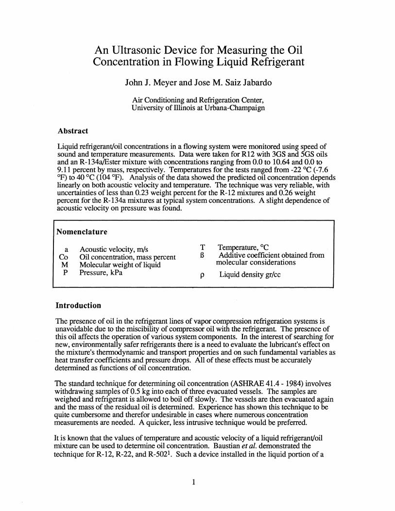
Abstract

Liquid refrigerant/oil concentrations in a flowing system were monitored using speed of sound and temperature measurements. Data were taken for R12 with 3GS and 5GS oils and an R-134a/Ester mixture with concentrations ranging from 0.0 to 10.64 and 0.0 to 9.11 percent by mass, respectively. Temperatures for the tests ranged from -22°C (-7.6 OF) to 40 °C (104 OF). Analysis of the data showed the predicted oil concentration depends linearly on both acoustic velocity and temperature. The technique was very reliable, with uncertainties ofless than 0.23 weight percent for the R-12 mixtures and 0.26 weight percent for the R-134a mixtures at typical system concentrations. A slight dependence of acoustic velocity on pressure was found.

Nomenclature

a Acoustic velocity, mls Co Oil concentration, mass percent M Molecular weight of liquid

T Temperature, °C B Additive coefficient obtained from

molecular considerations P Pressure, kPa p Liquid density gr/cc

Introduction

The presence of oil in the refrigerant lines of vapor compression refrigeration systems is unavoidable due to the miscibility of compressor oil with the refrigerant The presence of this oil affects the operation of various system components. In the interest of searching for new, environmentally safer refrigerants there is a need to evaluate the lubricant's effect on the mixture's thermodynamic and transport properties and on such fundamental variables as heat transfer coefficients and pressure drops. All of these effects must be accurately determined as functions of oil concentration.

The standard technique for determining oil concentration (ASHRAE 41.4 - 1984) involves withdrawing samples of 0.5 kg into each of three evacuated vessels. The samples are weighed and refrigerant is allowed to boil off slowly. The vessels are then evacuated again and the mass of the residual oil is determined. Experience has shown this technique to be quite cumbersome and therefor undesirable in cases where numerous concentration measurements are needed. A quicker, less intrusive technique would be preferred.

It is known that the values of temperature and acoustic velocity of a liquid refrigerant/oil mixture can be used to determine oil concentration. Baustian et al. demonstrated the technique for R-12, R-22, and R-5021. Such a device installed in the liquid portion of a

1

test loop would measure oil concentration in real time without the need to withdraw a sample. The purpose of this study was to improve accuracy of the technique so it could be implemented in existing refrigerant test stands, and used to monitor transient migration of oil during cycling operation of a vapor-compression system.

Theory of Operation

If the transit time of a pressure wave which travels across a known path length is measured, the acoustic velocity can be calculated. This was accomplished in the liquid portion of a refrigerant test loop in the following way: A pulser/receiver sent a voltage to a 5 MHz ultrasonic transducer, which generated and detected pressure waves. These waves traveled through the flowing refrigerant/oil mixture, reflected off a polished surface, and returned to the transducer. This occurred within a brass housing device designed and constructed for this purpose (Figure 1). The pulser/receiver then conditioned the output voltage for an oscilloscope and a 225 MHz counter/timer. The counter/timer measured the time between the initial signal and the fIrst echo. Built-in mathematic functions converted this directly to acoustic velocity. The oscilloscope was used to monitor the signals and to watch for any abrupt changes. Two phase flow or immiscible oil attenuated the signal greatly, thereby alerting that the concentration of oil in solution was not representative of the overall concentration.

The housing device was designed to have replaceable transducers. Because the acoustic path length varies slightly with each transducer installation, the device must be recalibrated after each replacement. The calibration procedure consisted of immersing the housing device in distilled water within a constant temperature bath. Transit time measurements were taken at temperatures from 3 °C (37.4 OF) to 30°C (86.0 OF). Any effect of dissolved air was neglected2. From this data and a curve fit for the speed of sound in pure water a least squares fIt gave the best path length and associated uncertainty3. The device was then mounted in the test loop and measurements were taken. The accepted curve and predicted values are shown graphically in Figure 2. For the R-12 data the path length was 0.03379 meters. Installation of a new transducer for the R -134a data resulted in a path length of 0.03810 meters. After data were taken the housing device was recalibrated. The path length showed no signifIcant change.

Experimental Set-Up and Procedure

Major design considerations when constructing the test stand were control and measurement of pressure and temperature. A pressure regulator connected to a nitrogen tank was used to set the pressure within a bladder accumulator, and thus within the system. Pressure measurements were made with a pressure transmitter which utilized a variable capacitance technique. Because the loop was single phase liquid everywhere, large volume changes were avoided.

The temperature was adjusted with a chiller and a two kilowatt electric heater. Power to the heater was controlled with a variac. To avoid small temperature fluctuations due to heater or chiller cycling, most measurements were made with the heater and chiller operating, maintaining an energy balance at the desired temperature. The temperature was measured with type T thermocouples just upstream and downstream of the housing device. When a data point was taken these temperatures never differed by more then 0.2 °C (0.36 DC) and were almost always identical to 0.1 °C (0.18 OF) precision.

The upstream and downstream temperatures were monitored via a data acquisition system which showed both a digital value a plot of the temperature versus time. Mter adjusting the

2

temperature controls the refrigerant temperature at the test location was observed to approach the desired value asymptotically. Once the temperature curve was flat (± less than 0.1 °C) for approximately one minute, data was taken and new temperature adjustments made.

A positive displacement pump with variable speed control was used to control the flow rate. At several temperatures and concentrations the flow rate was varied to check for an effect on acoustic velocity. No effect was found. Due to heat transfer effects associated with the heater and chiller and pressure drop considerations in the mass flow meter the flow rate was maintained near 2000 gr/min.

Once the housing device was calibrated and the loop charged with pure refrigerant, acoustic velocity data were obtained across the temperature range. A small amount of oil and refrigerant were then added to the loop. Mter allowing for thorough mixing, measurements across the temperature span were repeated. ASHRAE Standard 41.4 - 1984 was used to determine the actual oil concentration for each repetition. The above procedure was repeated for several oil concentrations. The resulting data showed straight lines on an acoustic velocity versus temperature graph, with each line representing the corresponding measured oil concentration (Figure 3).

Transit time measurements

The transit time, which was on the order of 50 to 80 IlS, was represented on an oscilloscope screen by the time between voltage peaks corresponding to the initial signal and the following echoes. Baustian used this measuring procedure to determine the transit timel. This technique was attempted, but a simple propagation of error calculation showed it to be responsible for a large majority of the ±1.0 weight percent uncertainty reported.

Two alternative time measuring devices were then considered: A sing-around technique and a high accuracy timer/counter. The sing-around procedure consists of hardware which sends a voltage to the transducer every time it receives a voltage (previous signal echo). By monitoring the frequency of outgoing signals the period, and thus the transit time can be calculated4. The other option, a counter/timer, measures and displays digitally the time between two events. The counter/timer was chosen because of its off-the-shelf availability, accuracy, and ease of use.

Pressure Effects

Some difficulty was experienced in maintaining a constant amount of subcooling. For this reason the effect of pressure on acoustic velocity was investigated. Speed of sound measurements were made at a constant temperature as the pressure was varied from close to saturation to 1.4 MPa above saturation. This was done for temperatures ranging from -20°C (-4.0 OF) to 30°C (86.0 OF). For this range of subcooling, acoustic velocity was found to change linearly with pressure at a given temperature (Figure 4). A least squares analysis provided the slopes of the constant temperature lines as a function of temperature. When the value of this slope is multiplied by the pressure above saturation the increase in acoustic velocity relative to its saturation value is obtained. Effects on saturation pressure due to the presence of oil were neglected5. In his work Grebner showed the saturation pressure of R-12/paraffinic oil mixtures was unchanged from that of pure R-12 for oil concentrations below 11 %. The same trend was found for other refrigerant/oil mixtures. From this analysis it was determined that the acoustic velocity in liquid R-12 changed as a

3

function of temperature and pressure as follows:

a - asat = (0.00789 + 0.0000974*T)(P-Psat) (1)

The following similar expression was found for R-134a:

a - asat = (0.00830 + 0.000118*T)(P-Psat) (2)

As expected the acoustic velocity increases slightly with pressure. The above corrections were included when fitting the data. For typical subcooling in an actual vapor-compression system the correction term is negligible.

Results

Initial graphs of the data showed lines of constant oil concentration on an acoustic velocity versus temperature graph. As mentioned earlier, however, this technique is to be used for determining oil concentration. For this reason a single curve fit was developed to predict oil concentration as a function of temperature and acoustic velocity.

The initial correlation tested, Co=f(T(OC),asat(m!s)), included only three terms: a constant and two linear terms. Quadratic terms were then added one at a time until a complete quadratic model was attained. For each model a least squares technique found the best coefficients, a 95 percent confidence interval for each coefficient, and the associated model variance. From statistical F tests for the four correlations it was determined that the linear fit was sufficient with all three parameters being significant. The resulting linear correlation for a R-12/3GS mixture is:

Co = -75.63 + 0.1241asat + 0.4955T (3)

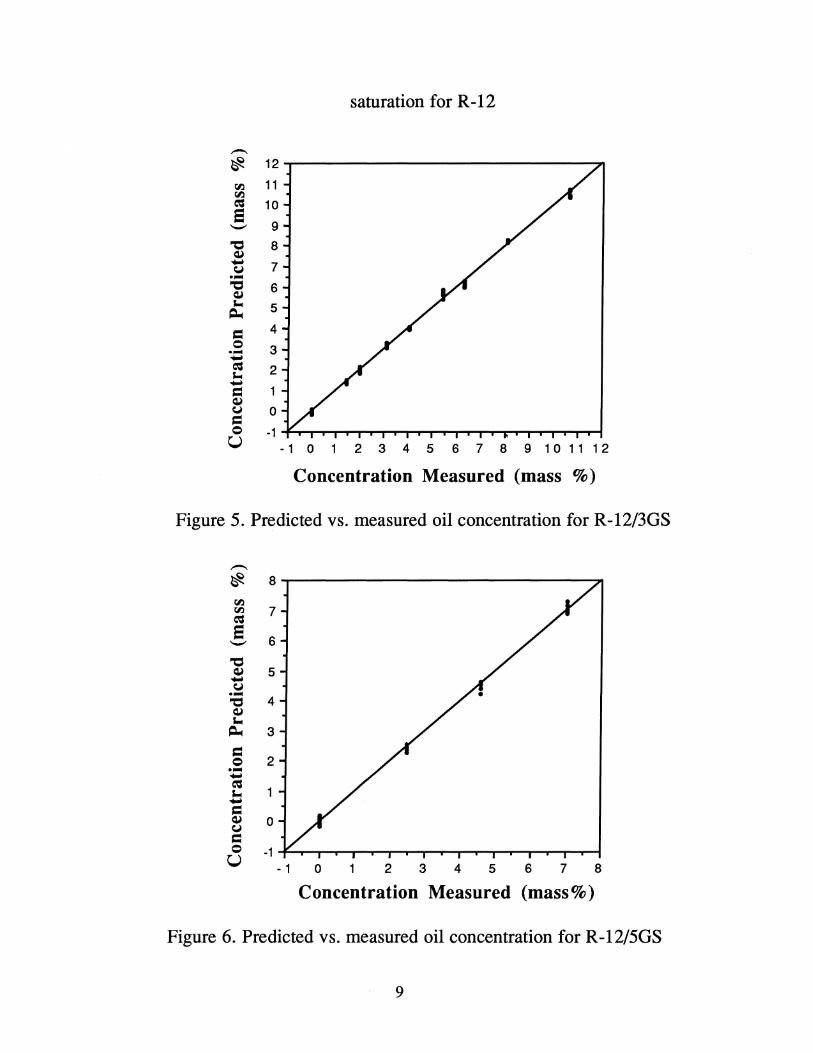
Predicted versus measured concentrations are shown in Figure 5. The uncertainty, based on a 95% confidence interval, in the above correlation is less than 0.23 weight percent for concentrations less than four percent and 0.42 weight percent for concentration between 4% and 10.64%. It is believed the higher uncertainty at concentrations greater than four percent is associated with the refrigerant/oil sampling procedure and not degradation of the speed of sound measurements. For this reason the uncertainty in the technique is most likely less than 0.42 weight percent for the higher concentrations. Due to the linear nature of the curve fit, it may be accurate for concentrations higher than 10.64% as well.

The same measurements and analysis were done for R-12 and 5GS oil. For this case, due to the linear nature of the correlation, fewer concentrations were investigated. It was hoped the same fit could be used for 3GS and 5GS oil. However, for R-12/5GS mixtures the obtained correlation was:

Co = -82.84 + 0.1361asat + 0.5447T (4)

The predicted versus measured concentrations for R12/5GS are shown in Figure 6. The uncertainty associated with the above fit is 0.26 weight percent based on a 95% confidence interval. This is close to the R-12/3GS fit, but generates errors of approximately two standard deviations at low concentrations and as much as ten standard deviations at 10.64% concentration if applied to the 3GS data.

The analysis was repeated for an R-134a/Ester mixture with the following result:

Co = -109.15 + 0.1762asat + 0.811OT (5)

4

Predicted and measured concentrations are shown in Figure 7. The uncertainty associated with the correlation is 0.26 weight percent based on a 95% confidence interval.

Discussion of Results

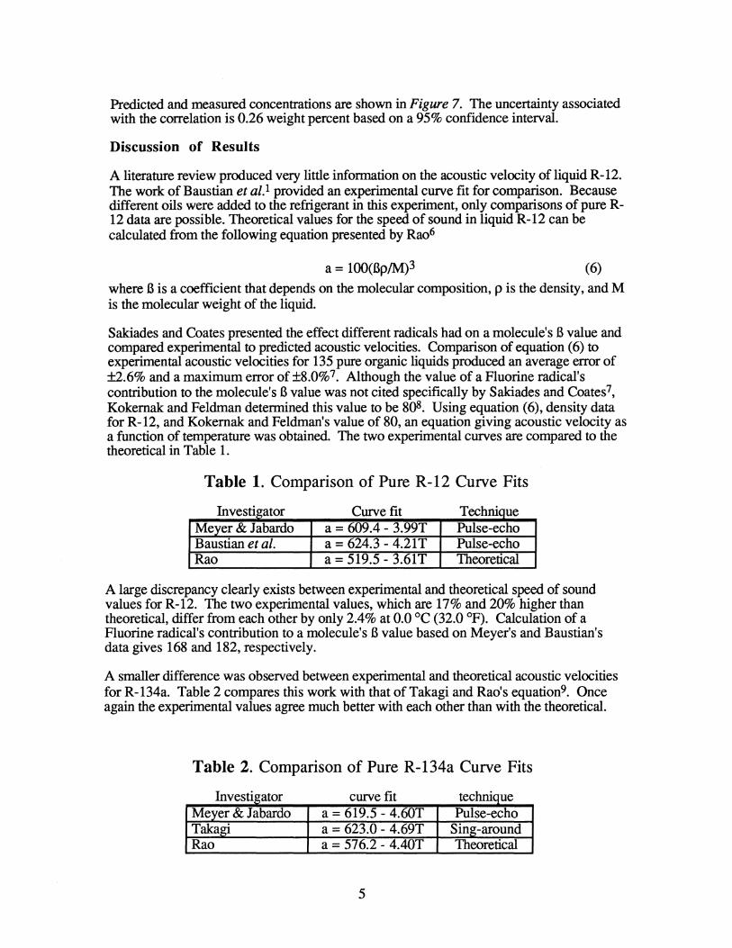
A literature review produced very little information on the acoustic velocity of liquid R-12. The work of Baustian et al. l provided an experimental curve fit for comparison. Because different oils were added to the refrigerant in this experiment, only comparisons of pure R-12 data are possible. Theoretical values for the speed of sound in liquid R-12 can be calculated from the following equation presented by Ra06

a = lOO(BplM)3 (6)

where B is a coefficient that depends on the molecular composition, p is the density, and M is the molecular weight of the liquid.

Sakiades and Coates presented the effect different radicals had on a molecule's B value and compared experimental to predicted acoustic velocities. Comparison of equation (6) to experimental acoustic velocities for 135 pure organic liquids produced an average error of ±2.6% and a maximum error of ±8.0% 7. Although the value of a Fluorine radical's contribution to the molecule's B value was not cited specifically by Sakiades and Coates7, Kokernak and Feldman determined this value to be 80s. Using equation (6), density data for R-12, and Kokernak and Feldman's value of 80, an equation giving acoustic velocity as a function of temperature was obtained. The two experimental curves are compared to the theoretical in Table 1.

Table 1. Comparison of Pure R-12 Curve Fits

In vestlgator C fi urve It T h . ec mque Me~er & labardo a = 609.4 - 3.99T Pulse-echo Baustian et al. a = 624.3 - 4.21 T Pulse-echo Rao a = 519.5 - 3.61T Theoretical

A large discrepancy clearly exists between experimental and theoretical speed of sound values for R-12. The two experimental values, which are 17% and 20% higher than theoretical, differ from each other by only 2.4% at 0.0 °C (32.0 OF). Calculation of a Fluorine radical's contribution to a molecule's B value based on Meyer's and Baustian's data gives 168 and 182, respectively.

A smaller difference was observed between experimental and theoretical acoustic velocities for R-134a. Table 2 compares this work with that of Takagi and Rao's equation9. Once again the experimental values agree much better with each other than with the theoretical.

Table 2. Comparison of Pure R-134a Curve Fits

I nvestlgator fi curve It tec hni Ique Meyer & 1 abardo a = 619.5 - 4.60T Pulse-echo Takagi a = 623.0 - 4.69T Sing-around Rao a = 576.2 - 4.40T Theoretical

5

In this case the two experimental values differ from the theoretical by 7.6% and from each other by 0.6% at 0.0 °C (32.0 oF). Calculation of a Fluorine radical's contribution to R-134a's B value based on Meyer's and Takagi's data gives 99 and 100, respectively. These data show that further investigation of the contribution from Fluorine radicals to B values is warranted.

Conclusion

The pulse-echo technique has been shown to be a practical and accurate technique to determine oil concentration in refrigerant flow. Small uncertainties along with online measurement capability makes the procedure very attractive. Although the procedure is limited to the liquid line where oil is completely dissolved, this technique for determining oil concentration may be useful for investigating the effect of oil on the performance of vapor-compression systems.

References

1 Baustian, J. J.; Pate, M. B.; and Bergles, A. E. Measuring the Concentration of a Flowing Oil-Refrigerant Mixture with an Acoustic Velocity Sensor ASH RAE Transactions (1988) 94 Part 2 602

2 Greenspan, M. and Tschiegg, C. Effect of Dissolved Air on the Speed of Sound in Water Journal of the Acoustical Society of America (1959) 28 501

3 Del Grosso, v. A. and Mader, C. W. Speed of sound in Pure Water Journal of the Acoustical Society of America (1972) 52 1442

4 Cedrone, N. P. and Curran, D. R. Electronic Pulse Method for Measuring the Velocity of Sound in Liquids and Solids Journal of the Acoustical Society of America (1954) 26963

5 Grebner, J. J. The Effects of Oil on the Thermodynamic Properties if Dichlorodifluoromethane (R-12) and Tetrafluoroethane (R-134a) ACRC TR-13 Air Conditioning and Refrigeration Center, University of Illinois at Urbana­Champaign, 1992.

6 Rao, M. R. Velocity of Sound in Liquids and Chemical Constitution Journal of Chemical Physics (1941) 9 682

7 Sakiadis, B. C. and Coates, J. Studies of Thermal Conductivity of Liquids A.l.Ch.E. Journal (1955) 1 275

8 Kokernak, R. P. and Feldman, C.L. The Velocity of Sound in Liquid R12ASHRAE Journal (1971) 13 59

9 Takagi, T. Personal communication 1991, cited in Thermophysical properties of Environmentally Acceptable Fluorocarbons Japanese Association of Rtfrigeration (1991)

6

.---GROVES FOR O-RINGS

Figure 1. Transducer Housing

1520

r:I.l 1500

e -= 1480

= = 0 00 1460 - Actual "-0

o Predicted

-= 1440 QJ QJ

c-oo

1420

1400 0 5 10 15 20 25 30 35

Temperature °C

Figure 2. Predicted and accepted acoustic velocity for water

7

800

A 10.64% 750 c 8.08%

t"I.l .. 5.22% -e 700 .6 3.10%

"0 • 1.41% CI 0 0.00% = 650 0

00 ~

600 0

"0 CIJ CIJ 550 C.

00

500

450 -30 -20 -10 0 1 0 20 30 40

Temperature °C

Figure 3. Constant oil concentration lines for R-12/3GS mixtures

12

10

,-.. 8 t"I.l -e '-'

= 6

<l

4 + 29.8°C c 22.0°C 0 -0.4 °C

2 0 -10.3°C .6 -20.3°C

0 0 200 400 600 800 1000 1200 1400

P-Psat (kPa)

Figure 4. Change in acoustic velocity vs. pressure above

8

saturation for R -12

.-~ 12

rI.l 11 rI.l = 10 E!

9 '-'

"0 8 ~ ....- 7 c:.J ....

"0 6 ~

'"" 5 ~

= 4 0 3 .... ....-= 2 '"" ....-= ~ c:.J 0

= 0 -1 U - 1 0 1 2 3 4 5 6 7 8 9 10 1112

Concentration Measured (mass %)

Figure 5. Predicted vs. measured oil concentration for R-12/3GS

.-~ 8

rI.l rI.l 7 = E! 6 '-'

"0 ~ ....- 5 c:.J ....

"0 4 ~

'"" ~ 3

= 2 0 .... ....-= '"" ....-= ~ 0 c:.J

= 0 -1 U - 1 0 1 2 3 4 5 6 7 8

Concentration Measured (mass%)

Figure 6. Predicted vs. measured oil concentration for R -12/5GS

9

~ 10

o -1~rT~~-r~~~~~~~~~-r~

-1 0 1 2 3 4 5 6 7 8 9 10

Concentration Measured (mass %)

Figure 7. Predicted vs. measured oil concentration for R -134a/Ester

10