an r package to process lc/ms metabolomic data: mait ... · allows users to perform end-to-end...

An R package to process LC/MS metabolomic data:

MAIT (Metabolite Automatic Identification Toolkit)

Francesc Fernandez-AlbertPolytechnic University

of CataloniaUniversity

ofBarcelona

Rafael LlorachUniversity

ofBarcelona

Cristina Andres-LacuevaUniversity

ofBarcelona

Alexandre PereraPolytechnic University

of Catalonia

Abstract

Processing metabolomic liquid chromatography and mass spectrometry (LC/MS) datafiles is time consuming. Currently available R tools allow for only a limited numberof processing steps and online tools are hard to use in a programmable fashion. Thispaper introduces the metabolite automatic identification toolkit MAIT package, whichallows users to perform end-to-end LC/MS metabolomic data analysis. The package isespecially focused on improving the peak annotation stage and provides tools to validatethe statistical results of the analysis. This validation stage consists of a repeated randomsub-sampling cross-validation procedure evaluated through the classification ratio of thesample files. MAIT also includes functions that create a set of tables and plots, suchas principal component analysis (PCA) score plots, cluster heat maps or boxplots. Toidentify which metabolites are related to statistically significant features, MAIT includesa metabolite database for a metabolite identification stage.

Keywords: Metabolomics, Peak Aggregation Measures, LC/MS.

1. Introduction

Liquid Chromatography and Mass Spectrometry (LC/MS) is an analytical instrument widelyused in metabolomics to detect molecules in biological samples (Theodoridis, Gika, Want,and Wilson 2012). It breaks the molecules down into pieces, some of which are detectedas peaks in the mass spectrometer. Metabolic profiling of LC/MS samples basically con-sists of a peak detection and signal normalisation step, followed by multivariate statisticalanalysis such as principal components analysis (PCA) and univariate statistical tests such asANOVA (Theodoridis et al. 2012; Tulipani, Llorach, Jauregui, Lopez-Uriarte, Garcia-Aloy,Bullo, Salas-Salvado, and Andres-Lacueva 2011).

2 MAIT (Metabolite Automatic Identification Toolkit)

As analysing metabolomic data is time consuming, a wide array of software tools are available,including commercial tools such as Analyst® software. There are programmatic R packages,such as XCMS (Smith, Want, O’Maille, Abagyan, and Siuzdak 2006; Tautenhahn, Bottcher,and Neumann 2008; Benton, Want, and Ebbels 2010) to detect peaks or CAMERA package(Kuhl, Tautenhahn, and Neumann 2011) and AStream (Alonso, Julia, Beltran, Vinaixa, Dıaz,Ibanez, Correig, and Marsal 2011), which cover only peak annotation. Another category offree tools available consists of those having online access through a graphical user interface(GUI), such as XCMS Online (http://xcmsonline.scripps.edu) or MetaboAnalyst (Xia,Psychogios, Young, and Wishart 2009), both extensively used.These online tools are difficult to use in a programmable fashion. They are also designedand programmed to be used step by step with user intervention, making it difficult to setup metabolomic data analysis workflow. These R packages involve only a part of the entiremetabolomic analysis process. Although there are specific R packages whose objective is peakannotation, this is still an issue in analysing LC/MS metabolomic data.

We introduce a new R package called metabolite automatic identification toolkit (MAIT) forautomatic LC/MS analysis. The goal of the MAIT package is to provide an array of toolsfor programmable metabolomic end-to-end analysis. It consequently has special functions toimprove peak annotation through the processes called biotransformations. Specifically, MAITis designed to look for statistically significant metabolites that separate the classes in the data.

2. Methodology

The main processing steps for metabolomic LC/MS data include the following stages: peakdetection, peak annotation and statistical analysis. In the peak detection stage, the objectiveis to detect the peaks in the LC/MS sample files. The peak annotation stage identifies themetabolites in the metabolomic samples better by increasing the chemical and biologicalinformation in the data set. A statistical analysis step is essential to obtain significant samplefeatures. All these 3 steps are covered in the MAIT workflow (see Figure 1).

2.1. Peak Detection

Peak detection in metabolomic LC/MS data sets is a complex issue for which several ap-proaches have been developed. Two of the most well established techniques are matched filter(Danielsson, Bylund, and Markides 2002) and the centWave algorithm (Tautenhahn et al.2008). MAIT can use both algorithms through the XCMS package.

2.2. Peak Annotation

The MAIT package uses 3 complementary steps in the peak annotation stage.

• The first annotation step uses a peak correlation distance approach and a retentiontime window to ascertain which peaks come from the same source metabolite, followingthe procedure defined at (Kuhl et al. 2011). The peaks within each peak group areannotated following a reference adduct/fragment table and a mass tolerance window.

• The second step uses a mass tolerance window inside the peak groups detected in the

http://xcmsonline.scripps.edu

Francesc Fernandez-Albert, Rafael Llorach, Cristina Andres-Lacueva, Alexandre Perera-Lluna 3

first step to look for more specific mass losses called biotransformations. To do this,MAIT uses a predefined biotransformation table where the biotransformations we wantto find are saved. A user-defined biotransformation table can be set as an input followingthe procedure defined in Section (4.6).

• The third annotation step is the metabolite identification stage, in which a predefinedmetabolite database is mined to search for the significant masses, also using a toler-ance window. This database is the Human Metabolome Database (HMDB) (Wishart,Knox, Guo, Eisner, Young, Gautam, Hau, Psychogios, Dong, Bouatra, and et al. 2009),2009/07 version.

2.3. Statistical Analysis

The objective of analysing metabolomic profiling data is to obtain the statistically sig-nificant features that contain the highest amount of class-related information. To gatherthese features, MAIT applies standard univariate statistical tests (ANOVA or Student’st-test) to every feature and selects the significant set of features by setting up a user-defined threshold P-value. Bonferroni multiple test correction can be applied to theresulting P-values.

We propose a validation test to quantify how well the data classes are separated by thestatistically significant features. The separation is validated through a repeated randomsub-sampling cross-validation using partial least squares and discriminant analysis (PLS-DA), support vector machine (SVM) with a radial Kernel and K-nearest neighbours(KNN) (Hastie, Tibshirani, and Friedman 2003). Overall and class-related classificationratios are obtained to evaluate the class-related information of the significant features.

2.4. Support for Peak Aggregation Techniques

MAIT optionally supports peak aggregation techniques that might lead to better featureselection (Fernandez-Albert, Llorach, Andres-Lacueva, and Perera 2011) through thecommercial pagR package.

3. MAIT workflow

MAIT accepts LC/MS files in the open formats mzData and netCDF. Sample filesshould be placed in a folder having a set of subfolders, each of which is going to be aclass in the data (see function sampleProcessing() in Section 4 for details).

The package centrepiece consists of the S4 MAIT-class objects. In terms of traceability,objects belonging to this class are designed to contain all the information related to theprocessing steps already run. The reason for this design is that using a single R objectthroughout the workflow improves the traceability of the analysis. The contents of aMAIT-class object are shown below. The slots of the MAIT-class objects are:

Formal class 'MAIT' [package "MAIT"] with 5 slots

..@ FeatureInfo:Formal class 'MAIT.FeatureInfo' [package "MAIT"] with

3 slots


.. .. ..@ biotransformations: logi [1, 1] NA

.. .. ..@ peakAgMethod : chr ""

.. .. ..@ metaboliteTable : logi [1, 1] NA

..@ RawData :Formal class 'MAIT.RawData' [package "MAIT"] with 2 slots

.. .. ..@ parameters:Formal class 'MAIT.Parameters' [package "MAIT"] with

9 slots

.. .. .. .. ..@ signalProcessing : list()

.. .. .. .. ..@ peakAnnotation : list()

.. .. .. .. ..@ peakAggregation : list()

.. .. .. .. ..@ sigFeatures : list()

.. .. .. .. ..@ biotransformations : list()

.. .. .. .. ..@ identifyMetabolites: list()

.. .. .. .. ..@ classification : list()

.. .. .. .. ..@ plotPCA : list()

.. .. .. .. ..@ plotHeatmap : list()

.. .. ..@ data : list()

..@ Validation :Formal class 'MAIT.Validation' [package "MAIT"] with 3

slots

.. .. ..@ ovClassifRatioTable: logi [1, 1] NA

.. .. ..@ ovClassifRatioData : list()

.. .. ..@ classifRatioClasses: logi [1, 1] NA

..@ PhenoData :Formal class 'MAIT.PhenoData' [package "MAIT"] with 3 slots

.. .. ..@ classes : logi(0)

.. .. ..@ classNum : logi(0)

.. .. ..@ resultsPath: chr ""

..@ FeatureData:Formal class 'MAIT.FeatureData' [package "MAIT"] with 7

slots

.. .. ..@ scores : logi [1, 1] NA

.. .. ..@ featureID : logi(0)

.. .. ..@ featureSigID : logi(0)

.. .. ..@ LSDResults : logi [1, 1] NA

.. .. ..@ models : list()

.. .. ..@ pvalues : logi(0)

.. .. ..@ pvaluesCorrection: chr ""

A MAIT-class object is built of 5 different S4 classes:

– FeatureInfo-class: The information regarding the peak annotation is saved inthis class.

– RawData-class: This class contains the data imported from the metabolomicLC/MS (xcmsSet-class object or xsAnnotate-class object depending on the lastfunction run)

– Validation-class: This contains the results of the cross-validation classificationstage.

– PhenoData-class: All the class-related information and the results path is con-tained in this class.


– FeatureData-class: This class contains the information related to the features,its P-values and the mathematical models used.

Figure 1 shows the flowchart of the main functions of the MAIT package, their outputfiles and their functionality. Table 1 shows the specific outputs of each function shownin Figure 1.

The MAIT package uses the wrapper function sampleProcessing() to call the re-quired XCMS functions to perform the peak detection step. These functions includexcmsSet(), group(), retcor() and fillPeaks(). The peaks detected are saved as axcmsSet-class object inside a MAIT-class object.


The default tables used to perform all the peak annotation steps are provided in MAITas an R Data object called MAITtables.RData. When this file is loaded, the followingobjects can be found:

– posAdducts: The possible annotations for the first annotation step when the po-larisation mode in the sample acquisition is set to positive.

– negAdducts: The possible annotations for the first annotation step when the po-larisation mode in the sample acquisition is set to negative.

– biotransformationsTable: This table contains the specific biotransformationsfor the second annotation step.

– Database: The metabolite database table to perform the metabolite identificationstage (third peak annotation step). This database is the Human MetabolomeDatabase (HMDB)(Wishart et al. 2009), 2009/07 version.

The MAIT package uses a CAMERA package wrapper function called peakAnnotation()

to perform the first step in the peak annotation stage. CAMERA groups the peaks us-ing a retention time window followed by a correlation cut-off approach. An adduct tableis required to launch this step. A user-defined adduct table or a MAIT default adducttable (posAdducts or negAdducts) can be selected. The user-defined table should becreated following the CAMERA adduct table layout, which is:

name nmol charge massdiff oidscore quasi ips

1 [M+H]+ 1 1 1.007276 1 1 1.0

2 [M+Na]+ 1 1 22.989218 8 1 1.0

3 [M+K]+ 1 1 38.963158 10 1 1.0

4 [M+NH4]+ 1 1 18.033823 16 1 1.0

5 [M+2Na-H]+ 1 1 44.971160 34 0 0.5

6 [M+2K-H]+ 1 1 76.919040 60 0 0.5


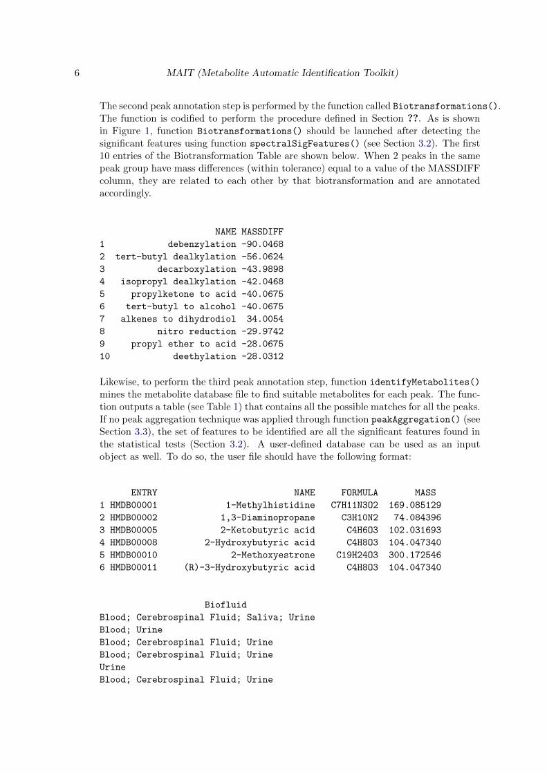
The second peak annotation step is performed by the function called Biotransformations().The function is codified to perform the procedure defined in Section ??. As is shownin Figure 1, function Biotransformations() should be launched after detecting thesignificant features using function spectralSigFeatures() (see Section 3.2). The first10 entries of the Biotransformation Table are shown below. When 2 peaks in the samepeak group have mass differences (within tolerance) equal to a value of the MASSDIFFcolumn, they are related to each other by that biotransformation and are annotatedaccordingly.

NAME MASSDIFF

1 debenzylation -90.0468

2 tert-butyl dealkylation -56.0624

3 decarboxylation -43.9898

4 isopropyl dealkylation -42.0468

5 propylketone to acid -40.0675

6 tert-butyl to alcohol -40.0675

7 alkenes to dihydrodiol 34.0054

8 nitro reduction -29.9742

9 propyl ether to acid -28.0675

10 deethylation -28.0312

Likewise, to perform the third peak annotation step, function identifyMetabolites()

mines the metabolite database file to find suitable metabolites for each peak. The func-tion outputs a table (see Table 1) that contains all the possible matches for all the peaks.If no peak aggregation technique was applied through function peakAggregation() (seeSection 3.3), the set of features to be identified are all the significant features found inthe statistical tests (Section 3.2). A user-defined database can be used as an inputobject as well. To do so, the user file should have the following format:

ENTRY NAME FORMULA MASS

1 HMDB00001 1-Methylhistidine C7H11N3O2 169.085129

2 HMDB00002 1,3-Diaminopropane C3H10N2 74.084396

3 HMDB00005 2-Ketobutyric acid C4H6O3 102.031693

4 HMDB00008 2-Hydroxybutyric acid C4H8O3 104.047340

5 HMDB00010 2-Methoxyestrone C19H24O3 300.172546

6 HMDB00011 (R)-3-Hydroxybutyric acid C4H8O3 104.047340

Biofluid

Blood; Cerebrospinal Fluid; Saliva; Urine

Blood; Urine

Blood; Cerebrospinal Fluid; Urine


Urine



Each of these 3 annotation steps is implemented through a function. These 3 functionsall have an input parameter where a user-defined table can be used instead of the MAITdefault tables. In particular, in function peakAnnotation() there is the argumentadductTable, in function Biotransformations(), the argument is called bioTable

and the input argument for function identifyMetabolites() is called database.


spectralSigFeatures() performs a univariate statistical test on each feature to gatherthe statistically significant variables that separate the classes in the data. The results ofthese statistical tests are saved in the MAIT-class object and are easily retrieved fromit by applying function sigPeaksTable(). The validation procedure defined in Section2.2 is launched using function Validation(). The overall and class-related classificationratios are saved in boxplots and tables (see Table 1) in the folder called ”Validation”.The confusion matrices for each iteration and classifier are saved in the folder named”Confusion Tables”.

3.3. Support for Peak Aggregation Techniques

The peak aggregation techniques, optional in MAIT workflow, are applied throughfunction peakAggregation(). This function allows the use of several different methodsto obtain the peak aggregation measures. If the chosen method is None, no otherpackages are required and no peak aggregation technique is applied. Any other validchoice (Mean, Single, PCA, NMF) requires the additional commercial package pagR(see Figure 1).

3.4. Statistical Plots

The package also contains functions that create statistical plots to evaluate analysisresults. These plots include 2D PCA score plots and an interactive 3D PCA scoreplot through function plotPCA(). The interactive 3D PCA score plot is generatedby the package rgl (Adler and Murdoch 2012). Function plotHeatmap() produces anarray of heat maps using different thresholds for the P-values and hierarchical clusteringdistances (Euclidean and Pearson’s; see Table 1), whereas Function plotBoxplot()

makes it possible to create a boxplot for each significant feature found. As is shown inFigure 1, all 3 functions require the significant features to be found to run the functionscorrectly and create the plots.


sampleProcessing

peakAnnotation

MAIT Functions FunctionalityOutput Files

peakAggregationOptional throughpagR package

spectra.csv

significantFeatures.csv

Peak Annotation

Peak Detection

Statistical Analysis

Peak Annotation

metaboliteTable.csv

Validation folder

PCA Scoreplots

Boxplots

Heatmaps

Peak Annotation

Statistical Analysis

Visualisation

Visualisation

Visualisation

spectralSigFeatures

Biotransformations

identifyMetabolites

Validation

plotPCA

plotBoxplot

plotHeatmap

Figure 1: Flowchart showing the main MAIT functions. Each box refers to a function andeach circle points to the output files created in the workflow. Dashed arrows show the outputfiles or plots generated by the functions; solid arrows refer to the possible metabolomic dataprocessing paths.


Tab

le1:

Tab

lesh

owin

gth

eoutp

ut

file

sge

ner

ated

by

the

mai

nMAIT

funct

ions

show

nin

Fig

ure

1.

MAIT

Function

Outp

utFileNam

eOutp

utty

pe

Desc

rip

tion

peakAnnotation

Sp

ectr

a.c

svT

ab

leT

his

tab

lesu

mm

ari

ses

the

corr

esp

ond

ence

bet

wee

np

eaks

an

dsp

ectr

a

spectralSigFeatures

sign

ifica

ntF

eatu

res.

csv

Tab

le

Inth

ista

ble

the

resu

lts

of

the

un

ivari

ate

test

sp

erfo

rmed

for

ever

yfe

atu

reand

the

info

rmati

on

of

the

pea

kan

nota

tion

are

saved

.

identifyMetabolites

met

ab

olite

Tab

le.c

svT

ab

le

This

table

sum

mari

ses

the

resu

lts

of

all

the

pre

vio

us

fun

ctio

ns

inth

ew

ork

flow

(see

Fig

ure

1),

incl

ud

ing

peakAnnotation,

spectralSigFeatures

and

Biotransformations.

The

poss

i-b

lem

etab

olite

iden

tifi

cati

on

matc

hes

are

als

oin

clud

edin

the

tab

le.

Sco

replo

tP

C12.p

ng

Plo

tT

his

file

conta

ins

the

PC

Asc

ore

plo

tfo

rP

rin

cipalC

om

pon

ent

1vs

Pri

nci

pal

Com

pon

ent

2

plotPCA

Sco

replo

tP

C13.p

ng

Plo

tT

his

file

conta

ins

the

PC

Asc

ore

plo

tfo

rP

rin

cipalC

om

pon

ent

1vs

Pri

nci

pal

Com

pon

ent

3

Sco

replo

tP

C23.p

ng

Plo

tT

his

file

conta

ins

the

PC

Asc

ore

plo

tfo

rP

rin

cipalC

om

pon

ent

2vs

Pri

nci

pal

Com

pon

ent

3

plotHeatmap

XD

ista

nce

Hea

tmap

pY

.pn

gP

lots

This

set

of

file

sco

nta

inth

eh

eat

maps

aft

erap

ply

ing

ah

ier-

arc

hic

al

clu

ster

ing

usi

ng

Xd

ista

nce

(X=

Eu

clid

ean

or

Corr

e-la

tion

)an

dY

P-v

alu

e(Y

=0.0

5,

0.0

1,

0.0

01,

1e-

4,

1e-

5)

plotBoxplot

Boxplo

tsp

ectr

aX

.png

Plo

tsT

his

set

of

file

sco

nta

ina

boxp

lot

for

each

sign

ifica

nt

featu

refo

und

inth

eanaly

sis.

Con

fusi

on

Tab

les

Fold

erF

old

erw

her

eth

eC

onfu

sion

matr

ices

for

ever

yit

erati

on

step

are

saved

Boxplo

tC

lase

sC

lass

ifica

tion

.png

Plo

tB

oxplo

tsh

ow

ing

the

class

ifica

tion

rati

ofo

rea

chcl

ass

an

dcl

as-

sifier

Validation

Boxplo

tO

ver

all

Cla

ssifi

cati

on

.png

Plo

tB

oxplo

tsh

ow

ing

the

class

ifica

tion

rati

ofo

rcl

ass

ifier

regard

less

of

the

class

es.

Cla

ssifi

cati

on

Tab

leC

lass

X.c

svT

ab

les

Tab

lesh

ow

ing

the

class

ifica

tion

rati

os

for

each

class

ifier

an

dfo

rcl

ass

X.T

her

eon

eof

thes

eta

ble

sfo

rea

chcl

ass

inth

edata

.

Cla

ssifi

cati

on

Tab

le.c

svT

ab

leT

ab

lesh

ow

ing

the

over

all

class

ifica

tion

rati

os

for

each

class

ifier

regard

less

of

the

class

es.


Figure 2: Example of the correct sample distribution for MAIT package use. Each samplefile has to be saved under a folder with its class name.

4. Using MAIT

The data files for this example are a subset of the data used in reference (Saghatelian,Trauger, Want, Hawkins, Siuzdak, and Cravatt 2004), which are freely distributedthrough the XCMS package. In these data there are 2 classes of mice: a group wherethe fatty acid amide hydrolase gene has been suppressed (class knockout or KO) anda group of wild type mice (class wild type or WT). There are 6 spinal cord samples ineach class. In the following, the MAIT package will be used to read and analyse thesesamples using the main functions discussed in Section 3. The significant features relatedto each class will be found using statistical tests and analysed through the different plotsthat MAIT produces.

4.1. Data Import

Each sample class file should be placed in a directory with the class name. All the classfolders should be placed under a directory containing only the folders with the files tobe analysed. In this case, 2 classes are present in the data. An example of correct filedistribution using the example data files is shown in Figure 2.

4.2. Peak Detection

Once the data is placed in 2 subdirectories of a single folder, the function sampleProcessing()

is run to detect the peaks, group the peaks across samples, perform the retention timecorrection and carry out the peak filling process. As function sampleProcessing() usesthe XCMS package to perform these 4 processing steps, this function exposes XCMSparameters that might be modified to improve the peak detection step. A project nameshould be defined because all the tables and plots will be saved in a folder using thatname. For example, typing project = "project_Test", the output result folder willbe "Results_project_Test".

By choosing "MAIT_Demo" as the project name, the peak detection stage can be launched


by typing:

R> MAIT <- sampleProcessing(dataDir = "Dataxcms", project = "MAIT_Demo",

snThres=2,rtStep=0.03)

ko15: 215:366 230:680 245:1014 260:1392 275:1766 290:2120 305:2468 320:2804

335:3150 350:3468 365:3846 380:4182 395:4486 410:4804 425:5110 440:5444

455:5778 470:6136 485:6504 500:6892 515:7296 530:7742 545:8138 560:8620

575:9048 590:9526

ko16: 215:344 230:662 245:1018 260:1378 275:1728 290:2090 305:2434 320:2722

335:3030 350:3352 365:3680 380:4006 395:4310 410:4640 425:4966 440:5276

455:5618 470:6010 485:6370 500:6818 515:7230 530:7662 545:8108 560:8608

575:9110 590:9654

...

wt22: 215:304 230:568 245:872 260:1202 275:1536 290:1838 305:2150 320:2444

335:2758 350:3030 365:3306 380:3576 395:3848 410:4140 425:4420 440:4712

455:5018 470:5364 485:5692 500:6060 515:6472 530:6912 545:7326 560:7786

575:8302 590:8792

Peak detection done

262 325 387 450 512 575

Retention Time Correction Groups: 7

Warning: Span too small, resetting to 0.8

Retention time correction done

262 325 387 450 512 575

Peak grouping after samples done

ko15

Peak missing integration done

After having launched the sampleProcessing function, peaks are detected, they aregrouped across samples and their retention time values are corrected. A short summaryin the R session can be retrieved by typing the name of the MAIT-class object.

R> MAIT

A MAIT object built of 12 samples. No peak aggregation technique has been

applied

The object contains 6 samples of class KO

The object contains 6 samples of class WT


The result is a MAIT-class object that contains information about the peaks detected,their class names and how many files each class contains. A longer summary of the datais retrieved by performing a summary of a MAIT-class object. In this longer summaryversion, further information related to the input parameters of the whole analysis isdisplayed. This functionality is especially useful in terms of traceability of the analysis.

A MAIT object built of 12 samples. No peak aggregation technique has been

applied



Parameters of the analysis:

Value

dataDir "Dataxcms"

snThres "2"

Sigma "2.12332257516562"

mzSlices "0.3"

retcorrMethod "loess"

groupMethod "density"

bwGroup "3"

mzWidGroup "0.25"

filterMethod "matchedFilter"

rtStep "0.03"

nSlaves "0"

project "MAIT_Demo"

ppm "10"


The next step in the data processing is the first peak annotation step, which is per-formed through the peakAnnotation(). If the input parameter adductTable is notset, then the default MAIT table for positive polarisation will be selected. However, ifthe adductTable parameter is set to ”negAdducts”, the default MAIT table for negativefragments will be chosen instead. peakAnnotation function also creates an output table(see Table 1) containing the peak mass (in charge/mass units), the retention time (inminutes) and the spectral ID number for all the peaks detected. A call of the functionpeakAnnotation may be:

R> MAIT <- peakAnnotation(MAIT.object = MAIT,corr = 0.7, perfwhm = 0.6)


WARNING: No input adduct/fragment table was given.

Selecting default MAIT table for positive polarity...

Set adductTable equal to negAdducts to use the default MAIT table for

negative polarity

Start grouping after retention time.

Created 1037 pseudospectra.

Spectrum build after retention time done

Start grouping after correlation.

Generating EICs ..

Calculating peak correlations in 1037 Groups...

% finished: 10 20 30 40 50 60 70 80 90 100

Calculating peak correlations across samples.

% finished: 10 20 30 40 50 60 70 80 90 100

Object contains no isotope or isotope annotation!

Calculating graph cross linking in 1037 Groups...

% finished: 10 20 30 40 50 60 70 80 90 100

New number of ps-groups: 2402

xsAnnotate now has 2402 groups, instead of 1037

Spectrum number increased after correlation done

Generating peak matrix!

Run isotope peak annotation

% finished: 10 20 30 40 50 60 70 80 90 100

Isotopes found: 9

Isotope annotation done

Generating peak matrix for peak annotation!

Found and use user-defined ruleset!

Calculating possible adducts in 2402 Groups...

% finished: 10 20 30 40 50 60 70 80 90 100

Adduct/fragment annotation done

Because the parameter adductTable was not set in the peakAnnotation call, a warningwas shown informing that the default MAIT table for positive polarisation mode wasselected. The xsAnnotated object that contains all the information related to peaks,spectra and their annotation is stored in the MAIT object. It can be retrieved by typing:

R> rawData(MAIT)

$xsaFA

An "xsAnnotate" object!

With 2402 groups (pseudospectra)

With 12 samples and 2640 peaks

Polarity mode is set to: positive

Using automatic sample selection

Annotated isotopes: 9


Annotated adducts & fragments: 32

Memory usage: 9.21 MB


Following the first peak annotation stage, we want to know which features are different be-tween classes. Consequently, we run the function spectralSigFeatures().

R> MAIT <- spectralSigFeatures(MAIT.object = MAIT,pvalue=0.05,bonferroni=FALSE,

scale=FALSE)

It is worth mentioning that by setting the scale parameter to TRUE, the data will be scaledto have unit variance. A summary of the statistically significant features is created and savedin a table called significantFeatures.csv (see Table 1). It is placed inside the Tables subfolderlocated in the project folder. This table shows characteristics of the statistically significantfeatures, such as their P-value, the peak annotation or the expression of the peaks acrosssamples. This table can be retrieved at any time from the MAIT-class objects by typing theinstruction:

R> signTable <- sigPeaksTable(MAIT.object = MAIT, printCSVfile = FALSE)

R> head(signTable)

mz mzmin mzmax rt rtmin rtmax npeaks KO WT ko15 ...

610 300.2 300.1 300.2 56.36 56.18 56.56 17 6 3 4005711.4 ...

762 326.2 326.1 326.2 56.92 56.79 57.00 9 5 2 3184086.4 ...

885 348.2 348.1 348.2 56.95 56.79 57.15 14 4 2 320468.2 ...

1760 495.3 495.2 495.3 56.93 56.82 57.05 11 3 4 110811.4 ...

935 356.2 356.1 356.3 63.77 63.58 63.92 9 4 4 962224.6 ...

1259 412.2 412.1 412.3 68.61 68.44 68.81 16 4 3 113096.3 ...

isotopes adduct pcgroup P.adjust p

610 27 1 0.01748294 ...

762 [M+H]+ 325.202 31 1 0.01991433 ...

885 [M+Na]+ 325.202 31 1 0.16856322 ...

1760 31 1 0.96828618 ...

935 74 1 0.03310409 ...

1259 81 1 0.02240898 ...

The number of significant features can be retrieved from the MAIT-class object as follows:

R> MAIT

A MAIT object built of 12 samples and 2640 peaks.

No peak aggregation technique has been applied

106 of these peaks are statistically significant




4.5. Statistical Plots

Out of 2,402 features, 106 were found to be statistically significant. At this point, severalMAIT functions can be used to extract and visualise the results of the analysis. FunctionsplotBoxplot, plotHeatmap and plotPCA automatically generate boxplots, heat maps andPCA score plot files in the project folder when they are applied to a MAIT object (see Table1).

R> plotBoxplot(MAIT)

R> plotHeatmap(MAIT)

R> plotPCA(MAIT)

All the output figures are saved in their corresponding subfolders contained in the projectfolder. The names of the folders for the boxplots, heat maps and score plots are Boxplots,Heatmaps and PCA Scoreplots respectively. Figures 3 and 4 depict a heat map and a scoreplot created when functions plotHeatmap and plotPCA were launched. Inside the R session,the project folder is recovered by typing:

R> resultsPath(MAIT)

4.6. Biotransformations

Before identifying the metabolites, peak annotation can be improved using the functionBiotransformations to make interpreting the results easier. The MAIT package uses adefault biotransformations table, but another table can be defined by the user and introducedby using the bioTable function input variable. The biotransformations table that MAIT usesis saved inside the file MAITtables.RData, under the name biotransformationsTable.

R> MAIT <- Biotransformations(MAIT.object = MAIT, peakPrecision = 0.005)

WARNING: No input biotransformations table was given.

Selecting default MAIT table for biotransformations...

% Annotation in progress: 10 20 30 40 60 70 80 90 100

Building a user-defined biotransformations table from the MAIT default table or adding anew biotransformation is straightforward. For example, let’s say we want to add a new adductcalled ”custom biotrans” whose mass loss is 105.

R> data(MAITtables)

R> myBiotransformation<-c("custom_biotrans",105.0)

R> myBiotable<-biotransformationsTable

R> myBiotable[,1]<-as.character(myBiotable[,1])

R> myBiotable<-rbind(myBiotable,myBiotransformation)

R> myBiotable[,1]<-as.factor(myBiotable[,1])

R> tail(myBiotable)


Figure 3: Heat map created by the function plotHeatmap. Row numbers refer to spectranumbers.


Figure 4: PCA score plot generated by the function plotPCA. Classes are separated throughthe PC1 direction.

NAME MASSDIFF

45 glucuronide conjugation 176.0321

46 hydroxylation + glucuronide 192.0270

47 GSH conjugation 305.0682

48 2x glucuronide conjugation 352.0642

49 [C13] 1.0034

50 [IDEM] 0.0000

51 custom_biotrans 105.0

To build an entire new biotransformations table, you only need to follow the format of thebiotransformationsTable, which means writing the name of the biotransformations as factorsin the NAME field of the data frame and their corresponding mass losses in the MASSDIFF field.

4.7. Metabolite Identification

Once the biotransformations annotation step is finished, the significant features have beenenriched with a more specific annotation. The annotation procedure performed by theBiotransformations() function never replaces the peak annotations already done by otherfunctions. MAIT considers the peak annotations to be complementary; therefore, when newannotations are detected, they are added to the current peak annotation and the identifica-tion function may be launched to identify the metabolites corresponding to the statisticallysignificant features in the data.

R> MAIT <- identifyMetabolites(MAIT.object = MAIT, peakTolerance = 0.005)


WARNING: No input database table was given.

Selecting default MAIT database...

Metabolite identification initiated

% Metabolite identification in progress: 10 20 30 40 50 60 70

80 90 100

Metabolite identification finished

By default, the function identifyMetabolites() looks for the peaks of the significant fea-tures in the MAIT default metabolite database. The input parameter peakTolerance de-fines the tolerance between the peak and a database compound to be considered a possiblematch. It is set to 0.005 mass/charge units by default. To check the results easily, functionidentifyMetabolites creates a table containing the significant feature characteristics andthe possible metabolite identifications. Such a table is recovered from the MAIT-class objectusing the instruction:

R> metTable <- metaboliteTable(MAIT)

R> head(metTable)

Query Mass Database Mass (neutral mass) rt Isotope Adduct

1 300.2 Unknown 56.36

2 588.2 Unknown 46.65

3 537.4 Unknown 64.41

4 451.2 450.193634 61.88

5 325.2 Unknown 60.95

6 395.1 Unknown 51.19

Name spectra Biofluid ENTRY p.adj (Bonferroni)

1 Unknown 27 unknown unknown 1



4 Geranylgeranyl-PP 1895 Not Available HMDB04486 0.393337



p Fisher KO_WT_NA_WT KO WT ko15 ko16 ko18 ko19 ko21

1 0.017482939 <NA> 6 3 4005711 3115028 2726906 2812957 57169

2 0.193607894 <NA> 2 4 0 0 0 0 2837

3 0.024657677 <NA> 1 3 0 0 0 0 0

4 0.003172073 <NA> 5 0 10878 1943 12670 9634 8338

5 0.019582285 <NA> 5 6 9563 7485 3538 11418 6814

6 0.025496645 <NA> 0 4 0 1801 3595 0 3386

ko22 wt15 wt16 wt18 wt19 wt21 wt22

1 832330 192385 94036 48410 137248 213369 85318

2 9154 40379 0 0 6697 13370 113071

3 3132 3307 0 4256 1844 4196 5967

4 9654 1671 3877 0 0 4226 0

5 7867 17010 18557 27223 7556 11949 18616

6 0 4896 9046 11105 5371 0 8033


This table provides useful results about the analysis of the samples, such as the P-value ofthe statistical test, its adduct or isotope annotation and the name of any possible hit in thedatabase. Note that if no metabolite has been found in the database for a certain feature, itis labelled as "unknown" in the table.

4.8. Validation

Finally, we will use the function Validation() to check the predictive value of the significantfeatures. All the information related to the output of the Validation() function is saved inthe project directory in a folder called ”Validation”. Two boxplots showing the overall andper class classification ratios are created, along with every confusion matrix corresponding toeach iteration (see Table 1).

R> MAIT <- Validation(Iterations = 20, trainSamples= 3, MAIT.object = MAIT)

Iteration 1 done

Iteration 2 done

Iteration 3 done

...

Iteration 19 done

Iteration 20 done

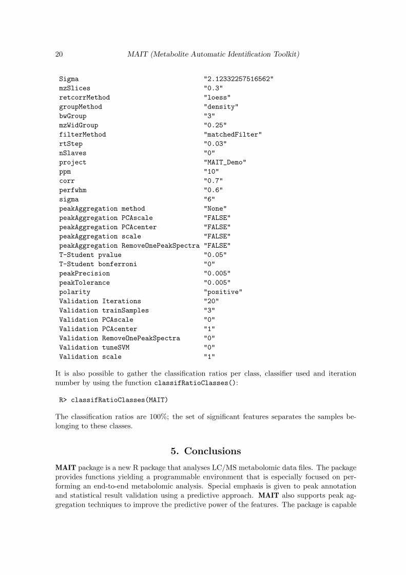
A summary of a MAIT object, which includes the overall classification values, can be accessed:

R> summary(MAIT)

A MAIT object built of 12 samples and 2640 peaks. No peak aggregation

technique has been applied

106 of these peaks are statistically significant



The Classification using 3 training samples and 20 Iterations gave

the results:

KNN PLSDA SVM

mean 1 1 1

standard error 0 0 0

Parameters of the analysis:

Value

dataDir "Data"

snThres "2"


Sigma "2.12332257516562"

mzSlices "0.3"

retcorrMethod "loess"

groupMethod "density"

bwGroup "3"

mzWidGroup "0.25"

filterMethod "matchedFilter"

rtStep "0.03"

nSlaves "0"

project "MAIT_Demo"

ppm "10"

corr "0.7"

perfwhm "0.6"

sigma "6"

peakAggregation method "None"

peakAggregation PCAscale "FALSE"

peakAggregation PCAcenter "FALSE"

peakAggregation scale "FALSE"

peakAggregation RemoveOnePeakSpectra "FALSE"

T-Student pvalue "0.05"

T-Student bonferroni "0"

peakPrecision "0.005"

peakTolerance "0.005"

polarity "positive"

Validation Iterations "20"

Validation trainSamples "3"

Validation PCAscale "0"

Validation PCAcenter "1"

Validation RemoveOnePeakSpectra "0"

Validation tuneSVM "0"

Validation scale "1"

It is also possible to gather the classification ratios per class, classifier used and iterationnumber by using the function classifRatioClasses():

R> classifRatioClasses(MAIT)

The classification ratios are 100%; the set of significant features separates the samples be-longing to these classes.

5. Conclusions

MAIT package is a new R package that analyses LC/MS metabolomic data files. The packageprovides functions yielding a programmable environment that is especially focused on per-forming an end-to-end metabolomic analysis. Special emphasis is given to peak annotationand statistical result validation using a predictive approach. MAIT also supports peak ag-gregation techniques to improve the predictive power of the features. The package is capable


of producing a set of post-processing plots, such as PCA score plots, and summary tablesto evaluate the results of the analysis. In short, MAIT is an easy, quick-to-use package forperforming a complete automatic analysis of LC/MS metabolomic data files.

6. Acknowledgements

This research was supported by Spanish national grants AGL2009-13906-C02-01/ALI, AGL2010-10084-E, the CONSOLIDER INGENIO 2010 Programme and FUN-C-FOOD (CSD2007-063)under the MICINN, as well as Merck Serono 2010 Research Grants (Fundacion Salud 2000).R. Llorach thanks the MICINN and The European Social Funds for their financial contri-bution to the R. L. Ramon y Cajal contract (Ramon y Cajal Programme, MICINN-RYC).This work has been partially supported by the Spanish Ministerio de Ciencia y Tecnologıathrough the TEC2010-20886-C02-02 and TEC2010-20886-C02-01 grants, and the Ramon yCajal programme. A. Perera is part of the 2009SGR-1395 consolidated research group ofthe Generalitat de Catalunya, Spain. CIBER-BBN is an initiative of the Spanish ISCIII. F.Fernandez-Albert thanks EVALXARTA-UB and Agencia de Gestio d’Ajuts Universitaris I deRecerca, AGAUR (Generalitat de Catalunya) for their financial support.

References

Adler D, Murdoch D (2012). rgl: 3D visualization device system (OpenGL). R package version0.92.894, URL http://CRAN.R-project.org/package=rgl.

Alonso A, Julia A, Beltran A, Vinaixa M, Dıaz M, Ibanez L, Correig X, Marsal S (2011).“AStream: an R package for annotating LC/MS metabolomic data.” Bioinformatics, 27(9),1339–1340. URL http://www.ncbi.nlm.nih.gov/pubmed/21414990.

Benton HP, Want EJ, Ebbels TMD (2010). “Correction of mass calibration gaps in liquidchromatography-mass spectrometry metabolomics data.” Bioinformatics, 26(19), 2488–2489. URL http://www.ncbi.nlm.nih.gov/pubmed/20671148.

Danielsson R, Bylund D, Markides KE (2002). “Matched filtering with background sup-pression for improved quality of base peak chromatograms and mass spectra in liquidchromatography-mass spectrometry.” Analytica Chimica Acta, 454(2), 167–184. URLhttp://linkinghub.elsevier.com/retrieve/pii/S0003267001015744.

Fernandez-Albert F, Llorach R, Andres-Lacueva C, Perera A (2011). “Un nuevo algoritmopara el analisis de estudios de nutrimetabolomica basados en LC-MS.” In Libro de actas:CASEIB 2011: XXIX Congreso Anual de la Sociedad Espanola de Ingenierıa Biomedica.

Hastie T, Tibshirani R, Friedman JH (2003). The Elements of Statistical Learning. Correctededition. Springer. ISBN 0387952845. URL http://www.worldcat.org/isbn/0387952845.

Kuhl C, Tautenhahn R, Neumann S (2011). “LC-MS Peak Annotation and Identification withCAMERA.” Camera, pp. 1–14.

Saghatelian A, Trauger SA, Want EJ, Hawkins EG, Siuzdak G, Cravatt BF (2004). “Assign-ment of endogenous substrates to enzymes by global metabolite profiling.” Biochemistry,43(45), 14332–14339. URL http://www.ncbi.nlm.nih.gov/pubmed/15533037.

http://CRAN.R-project.org/package=rgl

http://www.ncbi.nlm.nih.gov/pubmed/21414990


http://linkinghub.elsevier.com/retrieve/pii/S0003267001015744

http://www.worldcat.org/isbn/0387952845



Smith CA, Want EJ, O’Maille G, Abagyan R, Siuzdak G (2006). “XCMS: process-ing mass spectrometry data for metabolite profiling using nonlinear peak alignment,matching, and identification.” Analytical Chemistry, 78(3), 779–787. ISSN 00032700.doi:10.1021/ac051437y. URL http://pubs3.acs.org/acs/journals/doilookup?in_

doi=10.1021/ac051437y.

Tautenhahn R, Bottcher C, Neumann S (2008). “Highly sensitive feature detection for highresolution LC/MS.” BMC Bioinformatics, 9(1), 504. URL http://www.ncbi.nlm.nih.

gov/pubmed/19040729.

Theodoridis Ga, Gika HG, Want EJ, Wilson ID (2012). “Liquid chromatography-mass spec-trometry based global metabolite profiling: a review.” Analytica chimica acta, 711, 7–16.ISSN 1873-4324. doi:10.1016/j.aca.2011.09.042.

Tulipani S, Llorach R, Jauregui O, Lopez-Uriarte P, Garcia-Aloy M, Bullo M, Salas-SalvadoJ, Andres-Lacueva C (2011). “Metabolomics Unveils Urinary Changes in Subjects withMetabolic Syndrome following 12-Week Nut Consumption.” Journal of Proteome Research.ISSN 15353907. doi:10.1021/pr200514h. URL http://www.ncbi.nlm.nih.gov/pubmed/

21905751.

Wishart DS, Knox C, Guo AC, Eisner R, Young N, Gautam B, Hau DD, Psychogios N, DongE, Bouatra S, et al (2009). “HMDB: a knowledgebase for the human metabolome.” NucleicAcids Research, 37(Database issue), D603–D610. URL http://www.pubmedcentral.nih.

gov/articlerender.fcgi?artid=2686599&tool=pmcentrez&rendertype=abstract.

Xia J, Psychogios N, Young N, Wishart DS (2009). “MetaboAnalyst: a web server formetabolomic data analysis and interpretation.” Nucleic Acids Research, 37(suppl 2),W652–W660. doi:10.1093/nar/gkp356. http://nar.oxfordjournals.org/content/

37/suppl_2/W652.full.pdf+html, URL http://nar.oxfordjournals.org/content/

37/suppl_2/W652.abstract.

Affiliation:

Francesc Fernandez-Albert and Alexandre PereraDepartment d’Enginyeria de Sistemes, Automatica i Informatica IndustrialUniversitat Politecnica de CatalunyaBarcelona, SpainE-mail: [email protected]@upc.edu

Francesc Fernandez-Albert, Rafael Llorach and Cristina Andres-LacuevaNutrition and Food Science Department, XaRTA INSA, INGENIO-CONSOLIDER Program,FUN-C-Food CSD2007-063Avinguda Joan XXIII sn, 08028 BarcelonaPharmacy SchoolUniversity of Barcelona, SpainBarcelona, Spain

http://dx.doi.org/10.1021/ac051437y

http://pubs3.acs.org/acs/journals/doilookup?in_doi=10.1021/ac051437y

http://pubs3.acs.org/acs/journals/doilookup?in_doi=10.1021/ac051437y



http://dx.doi.org/10.1016/j.aca.2011.09.042

http://dx.doi.org/10.1021/pr200514h



http://www.pubmedcentral.nih.gov/articlerender.fcgi?artid=2686599&tool=pmcentrez&rendertype=abstract

http://www.pubmedcentral.nih.gov/articlerender.fcgi?artid=2686599&tool=pmcentrez&rendertype=abstract

http://dx.doi.org/10.1093/nar/gkp356

http://nar.oxfordjournals.org/content/37/suppl_2/W652.full.pdf+html

http://nar.oxfordjournals.org/content/37/suppl_2/W652.full.pdf+html

http://nar.oxfordjournals.org/content/37/suppl_2/W652.abstract

http://nar.oxfordjournals.org/content/37/suppl_2/W652.abstract

mailto:[email protected]



E-mail: [email protected]@ub.edu



an r package to process lc/ms metabolomic data: mait ... · allows users to perform end-to-end...

Documents