an overview of geographically discontinuous …

AN OVERVIEW OF

GEOGRAPHICALLY

DISCONTINUOUS TREATMENT

ASSIGNMENTS WITH AN

APPLICATION TO CHILDREN’S

HEALTH INSURANCE$

Luke Keelea, Scott Lorchb, Molly Passarellab,

Dylan Smallc and Rocı́o Titiunikd

aGeorgetown University, Washington, DC, USAbThe Children’s Hospital of Philadelphia and School of Medicine,University of Pennsylvania, Philadelphia, PA, USAcDepartment of Statistics, University of Pennsylvania, Philadelphia,PA, USAdDepartment of Political Science, University of Michigan, Ann Arbor,MI, USA

Regression Discontinuity Designs: Theory and Applications

Advances in Econometrics, Volume 38, 147�194

Copyright r 2017 by Emerald Publishing Limited

All rights of reproduction in any form reserved

ISSN: 0731-9053/doi:10.1108/S0731-905320170000038007

147

$Authors are in alphabetical order.

ABSTRACT

We study research designs where a binary treatment changes discontinu-ously at the border between administrative units such as states, counties,or municipalities, creating a treated and a control area. This type of geo-graphically discontinuous treatment assignment can be analyzed in astandard regression discontinuity (RD) framework if the exact geo-graphic location of each unit in the dataset is known. Such data, how-ever, is often unavailable due to privacy considerations or measurementlimitations. In the absence of geo-referenced individual-level data, twoscenarios can arise depending on what kind of geographic information isavailable. If researchers have information about each observation’s loca-tion within aggregate but small geographic units, a modified RD frame-work can be applied, where the running variable is treated as discreteinstead of continuous. If researchers lack this type of information andinstead only have access to the location of units within coarse aggregategeographic units that are too large to be considered in an RD framework,the available coarse geographic information can be used to create a bandor buffer around the border, only including in the analysis observationsthat fall within this band. We characterize each scenario, and also dis-cuss several methodological challenges that are common to all researchdesigns based on geographically discontinuous treatment assignments.We illustrate these issues with an original geographic application thatstudies the effect of introducing copayments for the use of the Children’sHealth Insurance Program in the United States, focusing on the borderbetween Illinois and Wisconsin.

Keywords: Geographic discontinuity; natural experiment

1. INTRODUCTION

We study a form of research designs based on geography, where a treat-

ment changes discontinuously at the border between administrative units

such as states, counties, or municipalities. The opportunity to use designs

of this type is frequent given that policies often vary with the borders of

government or administrative units that are themselves based on geogra-

phy. Indeed, the extant literature contains numerous examples studying

148 LUKE KEELE ET AL.

the effect of pollution (Chen, Ebenstein, Greenstone, & Li, 2013), foreclo-sure laws (Pence, 2006), collective bargaining (Magruder, 2012), nationbuilding, governance and ethnic relations in Africa (Asiwaju, 1985; Berger,2009; Dell, 2010; Laitin, 1986; Michalopoulos & Papaioannou, 2014;Miguel, 2004; Miles, 1994; Miles & Rochefort, 1991; Posner, 2004), mediaeffects in Europe and the United States (Huber & Arceneaux, 2007;Kearney & Levine, 2014; Kern & Hainmueller, 2008; Krasno & Green,2008), local policies in U.S. cities (Gerber, Kessler, & Meredith, 2011),mosquito eradication (Salazar, Maffioli, Aramburu, & Agurto Adrianzen,2016), population shocks (Schumann, 2014), the effects of tax rates on resi-dential mobility (Young, Varner, Lurie, & Prisinzano, 2014), the effect ofprivate police forces (MacDonald, Klick, & Grunwald, 2016), and mobili-zation and polarization in the American electorate (Middleton & Green,2008; Nall, 2015.).

We discuss the general features of research designs based on a treatmentassignment that is geographically discontinuous, in particular how theimplementation of such designs is closely linked to the availability of geo-referenced information at the appropriate level. When the exact geographiclocation of each unit of analysis is available, the geographically discontinu-ous treatment assignment can be analyzed in a standard regression discon-tinuity (RD) setup (Hahn, Todd, & van der Klaauw, 2001; Imbens &Lemieux, 2008; Lee & Lemieux, 2010) with a two-dimensional runningvariable. However, the availability of this kind of information is limitedin many applications, often because of confidentiality or measurementreasons.

When geo-referenced data at the individual level is not available, thestandard RD framework cannot be readily applied. When this happens,there are at least two ways to proceed with the analysis. If researchers haveinformation about each observation’s location within aggregate but smallgeographic units, a modified RD framework can be applied, where the run-ning variable is treated as discrete instead of continuous. If insteadresearchers only have access to the location of units within coarse aggregategeographic units that are too large to be considered in an RD framework,the coarse geographic information can be used to create a band or bufferaround the border that contains observations within a maximum distancefrom the border; the analysis then only includes observations within thebuffer. In this scenario, the identification assumptions must be modifiedaccordingly.

In what follows, we discuss these issues in detail, and also review otherchallenges that arise in the study of geographically discontinuous treatment

149An Overview of Geographically Discontinuous Treatment Assignments

assignments such as multiple treatments that coincide at the border of

interest; the enhanced ability of subjects to sort very precisely around the

border; the possibility of interference between treated and control units due

to their spatial proximity; and the potential heterogeneity in treatment

effects along the border. Our discussion draws on Keele and Titiunik

(2015b), Keele and Titiunik (2016), and Keele, Titiunik, and Zubizarreta

(2015), where we explored in detail several types of geographic designs. The

geographic regression discontinuity (GRD) is a special case of an RD

design with multiple running variables (e.g., Dell, 2010), which is discussed

in general by Imbens and Zajonc (2011), Papay, Willett, and Murnane

(2011), Reardon and Robinson (2012), and Wong, Steiner, and Cook

(2013).We illustrate with an original geographic application that studies the

effect of introducing copayments for the use of the Children’s Health

Insurance Program (CHIP), a public health insurance program in the United

States that covers children in families with modest incomes. Specifically, we

study whether the introduction of copayments in Wisconsin’s CHIP in 2008

led to a decrease in the usage of health services, relative to a control group

of Illinois residents who live just across the state border and whose CHIP

program did not introduce copayments in the period under study.

2. EMPIRICAL APPLICATION: COPAYMENTS

IN THE CHIP

Approximately, 8.1 million or 11% of all children in the United States have

health insurance through the CHIP (Kaiser Family Foundation 2016). This

program provides health coverage for uninsured children in families with

modest incomes that are not low enough to qualify for Medicaid coverage.

Faced with a combination of serious budgetary crises and rapid growth in

health care spending over the years, many states have adopted cost-

containment strategies used in the private insurance sector, most predomi-

nantly the implementation of copayments. Between 2003 and 2012, only 1

state had instituted deductibles, but 20 states had made 65 copayment

changes, with 12 states instituting 23 new copayment policies for one or

more medical services such as inpatient stays, emergency department visits,

nonpreventive outpatient visits, and prescription drugs (Heberlein, Brooks,

Alker, Artiga, & Stephens, 2013).


Extant research shows that copayments tend to reduce overall healthspending in a limited number of studies in pediatrics (Haggerty, 1985;Leibowitz et al., 1985; Lohr et al., 1986; Valdez et al., 1985), but may alsoreduce potentially beneficial items such as medications (Campbell, Allen-Ramey, Sajjan, Maiese, & Sullivan, 2011). For example, in Alabama, theincrease in copayments in 2004 was associated with a 2.4% reduction in theuse of brand name drugs, a 1.4% decrease in generic drugs, and a 2.5%decrease in outpatient visits to physicians (Sen et al., 2012). Preventivehealth visits and inpatient visits temporarily declined after these copaymentchanges, but the effects did not persist over time, unlike the changes toother more discretionary services. Investigators found that demand forinpatient services was less price sensitive compared to demand for otherservices such as medications and outpatient visits (Sen et al., 2012).However, it is not known whether copayments for one type of service willchange the use of other health care services which are substitutes or com-plements. Moreover, this study relied on a single-state, before-and-afterdesign. The lack of a robust control group raises questions about the valid-ity of its estimated effects of copayment increases.

In February 2008, Wisconsin expanded its CHIP program, known asBadgerCare, to create a new program known as BadgerCare Plus (BCþ).BCþ operates as a single program with two insurance products. The first,known as the Standard Plan, operates as Wisconsin’s traditional Medicaidplan for enrollees with incomes less than the Federal Poverty Level. Thesecond insurance product, known as the Benchmark Plan, is for enrolleeswith incomes above 200% of the Federal Poverty Level. Premiums are sub-sidized until incomes exceed 300% of the Federal Poverty Level. Under theBenchmark Plan, enrollees cannot have been offered employer-sponsoredinsurance in the last 12 months or have the opportunity to gain employer-based coverage in the next 3 months. BCþ simplified eligibility rules andenrollment processes and included a marketing and outreach program.Finally, BCþ also added payments for many services for some enrollees,specifically those children under age 18 whose family income was at orbelow 100% of the Federal Poverty Line plus all enrollees in theBenchmark Plan (Department of Health and Family Services 2008b).

The new copayment amounts ranged from $1 for acute care visits; $3 forinpatient services; $1�5 for prescription drugs, typically $1�5 for generic andcompound drugs, $3 for brand name drugs, and $0.50 for over-the-counterdrugs; to $3 for emergency department visits that did not result in a hospitaladmission (Department of Health and Family Services, 2008a; Ross &Marks,2009). Copays were not added to well child visits, which are designed to


administer preventative care. Copayments have continued to be modifiedsince the enactment of this legislation, such that by January of 2011, the maxi-

mum copayment was increased to $15 for a nonpreventive outpatient visit

and $100 for an inpatient visit, but had dropped to $0 for emergency depart-ment visits (Heberlein, Brooks, Guyer, Artiga, & Stephens, 2011).

The BCþ program is emblematic of many changes in U.S. health policy.

These policy changes occur at the state level and may have significanteffects on target populations. Many such policy changes do not have a ran-

domized component to aid evaluation � but see Baicker et al. (2013) for an

exception. The standard research strategy for studying such policy changesis differences-in-differences (DID), but geography-based designs are a natu-

ral alternative.We use this policy change as a case study. Since Wisconsin did not enact

other legislation that may affect the use of health care, we seek to understandwhether the addition of copayments to the Wisconsin CHIP program chan-

ged health care utilization. During this period, states that border Wisconsinleft their CHIP programs intact and did not add copayments. While these

states are relatively similar to Wisconsin, one can readily imagine reasons

why health care utilization may differ across these states other than the addi-tion of copays in Wisconsin. Differences in health care usage may arise from

differences in health care training that may influence the type and quality of

care delivered by practitioners; differential access to inpatient or outpatientcare, particularly in the large urban centers in the two states; and differences

in the care quality available to children in different regions of each state

(Asch, Nicholson, Srinivas, Herrin, & Epstein, 2009).We treat the change in insurance copays as a treatment that changes

discontinuously at the Wisconsin state border. In our application, we use

residents from Illinois as the control group. With a geographic design, wecan compare families living close to the state border. This provides a more

similar control population than if we used larger state populations, as we

will demonstrate through a comparison of Wisconsin and Illinois childrenreceiving CHIP insurance.

3. DISCONTINUOUS ASSIGNMENT OF TREATMENT

AT A GEOGRAPHIC BOUNDARY

We focus on the general problem of studying the effect of a binary inter-

vention or treatment that (i) is given to all units in a geographic area, and


(ii) is withheld from all units who are located on the other side of this area’s

geographic boundary. In other words, the border between the treated and

control areas marks the boundary where the treatment assignment changes

discontinuously from zero to one. Under certain circumstances, this setup

can be analyzed by directly applying a generalization of the standard RD

framework. In other cases, typically when geo-located data is not available,

the standard RD machinery cannot be applied, and a natural experimental

framework may be used instead.We denote the binary treatment of interest by T, and assume we have a

random sample of n subjects or units, indexed by i ¼ 1, 2,…, n, from a larger

population. The treatment is assigned based on geography, so that all units

who are located in area At have Ti ¼ 1, and all units located in area Ac have

Ti ¼ 0. For example, in our health care usage application the treated area At

is Wisconsin, while the control area Ac is Illinois. Thus, Ti ¼ 1 if i resides in

Wisconsin and is subject to insurance copays, and Ti ¼ 0 if i resides in Illinois

and does not have copays. Note that the setup assumes that there are no

compliance problems, so that the treatment assignment and the actual treat-

ment received are identical for every unit.We adopt the potential outcomes framework and let each individual

have two potential outcomes, Yi1 and Yi0, which correspond to levels

of treatment Ti ¼ 1 and Ti ¼ 0, respectively. The observed outcome is

Yi ¼ TiYi1 þ (1�Ti)Yi0. We also assume that the Stable Unit Treatment

Value Assumption or SUTVA holds (Cox, 1958; Rubin, 1986). SUTVA is

comprised of two parts: there are no hidden forms of treatment, which

implies that for unit i under Ti ¼ t, we have Yit ¼ Yi; and the potential out-

comes of one unit do not depend on the treatment of other units. As we

outline later, the validity of both parts of SUTVA may be questionable in

geographic designs.Under this framework, the treatment is a deterministic function of the

unit’s geographic location. The analysis of this type of designs will there-

fore depend on whether the exact location of each individual in the sample

is known. We now consider the different types of parameters that can be

defined and estimated with and without this form of geo-located data.

3.1. GRD Designs When Data Is Geo-Located

If researchers have access to the exact geographic location of each unit, the

discontinuous treatment assignment based on geography can be analyzed

in a standard RD setup, with the only modification that the running


variable or score that determines treatment has two dimensions instead of

one (see Imbens & Zajonc, 2011; Papay et al., 2011; Wong et al., 2013).To consider this case, which we discussed in more detail in Keele and

Titiunik (2015b), we assume that each unit’s geographic location is

known and given by a pair of geographic coordinates such as longitude

and latitude. We define the two-dimensional score Si ¼ (Si1, Si2), which

records the geographic location of individual i given by the two geo-

graphic coordinates. We call the set that collects the locations of all

boundary points B, and denote a single point on the boundary by b, with

b ¼ S1; S2ð Þ∈B. Thus, At and Ac are sets that collect all the locations

that receive treatment and control, respectively. The treatment assignment

is Ti ¼ T(Si), with T(s) ¼ 1 for s ∈ At and with T(s) ¼ 0 for s ∈ Ac.

This assignment has a discontinuity at the known boundary B. We

assume that the density of Si, f(s), is positive and continuous in a neigh-

borhood of the boundary B � an assumption that is often particularly

restrictive in geographic contexts.Under this setup, a natural parameter of interest is τ(b) ≡ E[Yi1 � Yi0∣Si ¼

b], for b∈B. Since there is a (possibly different) treatment effect τ(b) for everypoint b on the boundary, this defines a treatment effect curve. Alternatively,

these effects can be averaged across all boundary points, leading to the

parameter τ ¼ E τ bð Þ∣b∈B½ �.Identification of τ(b) follows from generalizing the standard RD identifi-

cation results in Hahn et al. (2001) to a two-dimensional running variable.

Thus, the main assumption required for identification is continuity of con-

ditional regression functions E[Yi1∣s] and E[Yi0∣s], at all points on the

boundary. In the context of our application, this assumption implies that

the average potential health care utilization under a copayment regime for

a unit located near a point b on the Wisconsin�Illinois boundary is very

similar to the average utilization that would be observed exactly at this

boundary point, regardless of the direction in which we approach the

boundary. Thus, when data is geo-located, this design may be deemed a

GRD design, and it is a particular case of an RD design with two running

variables (Keele & Titiunik, 2015b). For example, the GRD design is math-

ematically equivalent to an RD design where students take two exams and

receive a treatment only if each of their two exam scores exceeds a known

(and possibly different) cutoff.When the relevant continuity conditions hold, the average treatment

effect at the cutoff can be identified as the limit of two regression functions

on the observed outcomes. In other words, letting superscripts t and c

denote locations in the treated and control areas, respectively, we have


τ bð Þ ¼ limst →bE Yi∣Si ¼ st½ � � limsc → bE Yi∣Si ¼ sc½ � for all b∈B, which isanalogous to the single-dimensional standard RD result.

The availability of geo-located data together with a continuous two-dimensional running variable and the assumption of continuity of the con-ditional regression functions means that standard smoothness-based RDmethods for estimation and inference can be applied directly to this prob-lem. In essence, geo-located data allows us to approximate the regressionfunctions arbitrarily close to any boundary point (assuming data density ispositive everywhere).

In particular, local polynomial methods (Fan & Gijbels, 1996) are nowstandard in the analysis of RD designs, and can be applied with appropri-ate modifications to the geographic setup we are considering here. For agiven point b on the boundary, we calculate a distance measure betweenthe location Si of unit i and the boundary point b. For every unit i in thesample, we define this distance as dib :¼ d(b, Si). For example, if Euclidean

distance is used, dib ¼ffiffiffiffiffiffiffiffiffiffiffiffiffiffiffiffiffiffiffiffiffiffiffiffiffiffiffiffiffiffiffiffiffiffiffiffiffiffiffiffiffiffiffiffiffiffiffiffib1 � Si1ð Þ2 þ b2 � Si2ð Þ2

q. Note that d(b, b) ¼ 0 by

definition.Letting

μ bð Þc ≡ limsc →b

E Yi0∣dib ¼ d b; scð Þ½ �;

μ bð Þt ≡ limst →b

E Yi1∣dib ¼ d b; stð Þ½ �;

we can estimate these functions by local linear regression. In order to doso, we solve

bαcb;bβc

b

� �¼ arg min

αcb;βcb

Xi∈Ac

Yi � αcb � βcbdib� �2

wib;

bαtb;bβ t

b

� �¼ arg min

αtb;βtb

Xi∈At

Yi � αtb � βtbdib� �2

wib;

where

wib ¼1

hbK

dib

hb

�

are spatial weights with K (⋅) representing a kernel weighting function and hba bandwidth. Note that the bandwidth is specific to each boundary point b;


thus, for implementation, a different bandwidth should be chosen at every b.Given these solutions, the GRD treatment effect is estimated as

bτðbÞ ¼ dμtðbÞ � dμcðbÞ ¼ bαtb � bαc

b:

Inference procedures must be implemented with care, as the standard

asymptotic distribution of the least-squares estimator and robust standard

errors ignore the asymptotic bias of the nonparametric local polynomial

estimator and lead to invalid inferences in general. The most common pro-

cedure of bandwidth selection is based on asymptotic mean-squared error

(MSE) minimization (see, e.g., Imbens & Kalyanaraman, 2012), a method

which leads to bandwidth choices that are too large for conventional confi-

dence intervals to be valid. In order to obtain valid inferences, researchers

may select a smaller bandwidth to undersmooth, a procedure that is ad hoc

and leads to power loss. An automatic, data-driven alternative is to esti-

mate the asymptotic bias ignored by conventional inference, and correct

the standard errors appropriately to produce robust confidence intervals

that are valid even for large bandwidths, including those selected by MSE

minimization (Calonico, Cattaneo, & Titiunik, 2014b). These methods are

implemented in the rdrobust software � see Calonico, Cattaneo, and

Titiunik (2014a) and Calonico, Cattaneo, Farrell, and Titiunik (2017) for

details on the STATA implementation, and Calonico, Cattaneo, and

Titiunik (2015) for details on the R implementation.1

In practice, since the boundary B is an infinite collection of points, we

can select a grid of G points along the boundary for estimation, b1, b2, …,

bG. For this grid of points, we define a series of treatment effects τ(bg) forg ¼ 1, 2, …, G. In this case, the estimation procedure leads to a collection

of G treatment effects that can vary along the boundary that separates the

treatment and control areas, and in fact leads to a treatment effect curve,

where each effect can then be mapped in its specific location, bg.

3.2. Geographic Treatment Assignments in the Absence of Geo-LocatedIndividual Data

When geo-located data is not available, the smoothing methods described

above cannot be applied, as there is no way to estimate the relevant regres-

sion functions arbitrarily close to the boundary. The unavailability of geo-

coded data is common in applications, typically caused by measurement


limitations or confidentiality restrictions. For example, in our application,

any information that allows the precise identification of individual patients

is removed from the data, and this naturally includes the exact address of

their residence.We now discuss two scenarios that may arise when the geo-location of

each individual observation is absent. In the first, the dataset contains geo-

graphic information for a sufficiently small unit, and an RD analysis can

proceed with some modifications. In the second, the geographic informa-

tion is too coarse; in this case, the analysis loses some of the distinctive RD

features.

3.2.1. Scenario 1: Geo-Location of Small Aggregate UnitsIn the first scenario, the researcher has information about each observa-

tion’s location within aggregate geographic units that are still sufficiently

small. For example, the data may contain information on each observa-

tion’s census block, the geo-location of which is often readily available.

Armed with this information, the researcher can then assign the census

block coordinates to each observation in the dataset, and treat those coor-

dinates as the RD running variable. The aggregation step in this strategy,

however, creates some complications because it causes all units in the same

aggregate unit to share the same coordinates and leads to mass points in

the running variable. This renders the standard RD methods discussed

above inapplicable, since such methods rely on the assumption of a contin-

uous score.An appropriate analysis of this scenario would involve RD methods that

allow for discrete running variables. One alternative is to use a randomization-

based RD framework, where instead of continuity one assumes that there is

a neighborhood or window around the cutoff where the treatment is as-if

randomly assigned. Implementation requires choosing the window where this

assumption plausibly holds, which can be done based on observable charac-

teristics of the units. These methods have been developed for standard RD

designs with a single score (see Cattaneo, Frandsen, & Titiunik, 2015;

Cattaneo, Titiunik, & Vazquez-Bare, 2017), but can be extended straightfor-

wardly to accommodate scores with two dimensions, and in particular to geo-

graphic RD applications where the window would be a geographic region.

This randomization-based method requires assumptions that are stronger

than the usual continuity assumptions invoked in the standard RD frame-

work � see Sekhon and Titiunik (2017) for an in-depth discussion of the local

randomization interpretation of RD designs.


An alternative strategy to deal with a discretized score is to approximatethe unknown regression function connecting the mass points in the runningvariable, and model the deviation between the expected and predicted out-come as a random specification error, as proposed by Lee and Card (2008).In practice, this strategy involves fitting a polynomial model of the outcomeon the score and clustering the standard errors by the discrete values of thescore. This can be adapted to the geographic case with a two-dimensionalscore; the implementation would include a polynomial on both dimensionsof the score and would cluster the standard errors by indicators corre-sponding to the aggregate geographic units where the mass points occur.Unlike the randomization-based method described above, this methodrequires a global fit and relies on the strong assumption that the specifica-tion errors are orthogonal to the score values.

3.2.2. Scenario 2: Geo-Location of Few Coarse Geographic UnitsThe second scenario occurs when the data contains information aboutaggregate geographic units that are simply too large to be considered in anRD framework. This occurs when researchers have coarse geographic infor-mation, and can only classify observations into a few categories accordingto their maximum distance to the boundary. Our application falls into thiscategory. For confidentiality reasons, we are unable to access patients’addresses or census block locations; instead, the smallest geographic unitcontained in the data is zip code. Aggregating the information to the zipcode level, however, is undesirable for various reasons. First, such aggrega-tion would dramatically reduce the sample size, as there are only 71 treatedzip codes contiguous to the segment of the Illinois�Wisconsin border weanalyze. Second, it would force us to conduct the analysis at an arbitrarylevel of aggregation, introducing the possibility of seeing a modifiable arealunit problem (MAUP) (Openshaw, 1984). MAUP refers to the fact thatareal units such as zip codes have borders that are relatively arbitrarywith respect to the spatial variation of the units measured. In this case,aggregate measures will not accurately reflect individual level phenomenaunless those phenomena are spatially constant with respect to the areal unit.Naturally, the biases caused by the MAUP would be avoided if we couldgeo-locate every observation in the dataset and use more spatially informa-tive measures.

What, then, is the appropriate strategy for analysis in this scenarioof coarse geographic information? One possibility is to treat the geographicallydiscontinuous treatment assignment as a natural experiment, and use thecoarse geographic information available to focus the analysis on treated and


control areas along the border that are sufficiently close to each other. Insome applications, geographically proximate treated and control areas are

similar to each other in other relevant dimensions, increasing the plausibility

of the analysis relative to a treated�control comparison that does not rely ongeographic information.

In this second scenario, the available geographic information can be

used in at least two ways. First, it can be used to select segments along theborder where the treated and control populations are comparable. This is

most relevant in cases where the boundary is long and contains some

segments that are, for example, unpopulated or overlapping with rivers ormountains that drastically separate and differentiate the treated and

control populations. For example, in our application, our treated area of

Wisconsin borders four states that do not have CHIP copayments, butonly the border with Illinois has enough population density to conduct the

analysis.The other way in which coarse geographic information can be used is

by only including in the analysis observations that are within a maximumdistance from the border. For example, we might only use units in zip

codes that are within 5 miles from the Wisconsin�Illinois border.Researchers can then invoke the assumption that, conditional on being in

this buffer around the boundary, potential outcomes and treatment

assignment are unrelated to each other, as we also discussed in Keele andTitiunik (2016). We can formalize this assumption by defining, for each

unit i in the dataset, the point on the border that is closest to i’s location

Si; we call this point b⋆i . We denote the distance between b⋆i and Si by

d⋆i :¼ d b⋆i ; Si�

; thus, d⋆i is the perpendicular distance between i’s location

and the border. The assumption that the comparison of treated andcontrol observations close to the border leads to valid inferences can be

formalized as follows:

Assumption 1 (Geographic Mean Independence). The potentialoutcomes Yi0, Yi1 are mean independent of the treatment assignmentTi within a buffer of length D > 0 around the border:

E½Yi1∣d⋆i <D; Ti� ¼ E½Yi1∣d⋆i <D�;E½Yi0∣d⋆i <D; Ti� ¼ E½Yi0∣d⋆i <D�:

In other words, by focusing on units that are close together, the preexist-

ing confounding differences between treated and control units can be


eliminated. This assumption is invoked often in applications that studythe effects of geographically discontinuous interventions, either formallyor informally (e.g., Card & Krueger, 1994; Lavy, 2010; Posner, 2004).2

Naturally, Assumption 1 is untestable, but researchers can nonethelessprovide some indirect empirical evidence consistent with its plausibility.Analogous to experimental settings, this assumption suggests that treatedand control units within the selected band should be similar in thoseobservable characteristics that are likely to be related to the potentialoutcomes. Thus, researchers should provide evidence that treated andcontrol units within the buffer are comparable in terms of relevantobservable characteristics that are determined before the treatment isassigned.

It is not uncommon, however, to encounter applications where, evenin a small band around the border, treated and control units differsignificantly in observable characteristics, questioning the plausibility ofAssumption 1. In this case, researchers must decide how to interpret thesedifferences. One alternative is to view the observable differences as a symp-tom of unsolvable differences between the groups, differences that are dueto “endogeneity” or “sorting” around the border and are likely to be pres-ent not only in observable but also in unobservable characteristics. In thiscase, the treatment effects estimated based on the geographically discontin-uous treatment assignment would lack credibility.

The other alternative is to assume that the predetermined observablecharacteristics available to the investigator capture enough of the treatmentassignment mechanism, so that conditioning on them would suffice tomake valid treated�control comparisons. Collecting in the vector Xi theavailable observable characteristics for each unit, this interpretationinvokes a weaker version of Assumption 1:

Assumption 2 (Conditional Geographic Mean Independence). Thepotential outcomes Yi0, Yi1 are conditionally mean independent ofthe treatment assignment Ti within a buffer of length D > 0 aroundthe border:

E Yi1∣d⋆i <D;Xi;Ti� � ¼ E Yi1∣d⋆i <D;Xi

� �;

E Yi0∣d⋆i <D;Xi;Ti� � ¼ E Yi0∣d⋆i <D;Xi

� �:

By invoking Assumption 2, which we also discussed in Keele et al.(2015), the researcher admits that focusing on a narrow band aroundthe border is not enough to create comparable groups, but she assumes


that a valid comparison can be made after one conditions on observablecharacteristics within this band. Following the terminology introduced by

Galiani, McEwan, and Quistorff (2017), we refer to research designs based

on assumptions such as 1 or 2 as geographic quasi-experiments (GQE).We use a GQE design in our health care utilization application, where we

find persistent observable differences between the populations on either sideof the Illinois�Wisconsin border. That is, we assume that the treatment is

as-if randomly assigned for those who live near the Illinois�Wisconsin

border, after conditioning on a set of pretreatment covariates. We address

the need to condition on covariates in more detail in the next section.

4. PARTICULARITIES OF TREATMENT

ASSIGNMENTS BASED ON GEOGRAPHY

In the previous section, we discussed the different scenarios that can arise

when geographically discontinuous treatment assignments are studied,focusing on the availability of geo-referenced information and how such

availability affects researchers’ ability to implement a pure RD framework.

In this section, we discuss some common challenges that arise in the analy-

sis of geographically discontinuous treatments that are common to all thescenarios discussed above. As we note, many of these challenges are specific

to geographically discontinuous treatments, as they rarely arise in nongeo-

graphic RD designs with two running variables.

4.1. Compound Treatments

When studying treatment assignments that change discontinuously at a

geographic border, it is common for multiple administrative or political

borders to perfectly overlap. When each of the overlapping borders inducesa change that can separately affect the outcome of interest, we face the

problem of “compound” treatments � a situation where two or more treat-

ments affect the outcome of interest simultaneously. Although this phe-

nomenon can also occur in standard RD designs (as when a person whoturns 65 becomes simultaneously eligible to multiple social programs), it is

more frequent in geographic treatment assignments because the border that

induces the change in the intervention is often an administrative border

that serves as a border for multiple units. For example, county borders


tend to coincide with the border of other relevant units such as school dis-tricts, congressional districts, media markets, and cities. In our application,the discontinuity of interest is the state border, which overlaps perfectlywith a city and county border.

Since the researcher is typically interested in the effect of a single inter-vention, compound treatments often pose a serious challenge and consti-tute a violation of the consistency component of SUTVA. When multipleborders overlap, absent any restrictions or assumptions, it will not be possi-ble to separate the effect of the treatment of interest on the outcome fromthe effect of all other simultaneous “irrelevant” treatments. In our currentapplication, we are unable to separate the effect of the new copays inWisconsin from any other treatments that change at the state border andalso affect health care utilization.

Keele and Titiunik (2015b) introduce the assumption of compoundtreatment irrelevance to address applications with compound treat-ments. To restate this assumption, we assume there are K binary treat-ments that coincide at the same geographic border. We denote thesetreatments as Tij, j ¼ 1, 2, …, K, for each individual i, with Tij ¼ {0, 1}.Only the kth treatment, Tik, is of interest. The potential outcomes nota-tion can be generalized to allow all K versions of treatment to possiblyaffect the potential outcomes of each individual: we let YiTi

be i’s poten-tial outcome, with Ti ¼ (Ti1, Ti2, …, Tik, …, TiK)

0. In order to isolate the

effect of Tik on the outcome of interest, we can invoke the followingassumption:

Assumption 3 (Compound Treatment Irrelevance). Assume the treat-ment of interest is the kth treatment. For each i and for all possiblepairs of treatment vectors Ti and T0

i, YiTi¼ YiT0

iif Tik ¼ T 0

ik.

When Assumption 3 holds, the potential outcomes are only a functionof the treatment of interest, so YiTi

¼ YiTikand we can go back to the origi-

nal notation, with Yi1 and Yi0 the potential outcomes corresponding,respectively, to Tik ¼ 1 and Tik ¼ 0. In many cases, potential outcomes willbe affected by each of these simultaneously occurring treatments, and iso-lating the effect of Tik will not be possible. The ideal situation occurs whenAssumption 3 can be avoided altogether because only the treatment ofinterest changes at the border. In some instances, analysts may also be ableto exploit variation in other dimensions such as time to disentangle thecompounded effects.

In our example, we must assume that there is no separate county effecton health care utilization, so that the county treatment can be exactly


reduced to the state treatment. Another alternative is to define the estimandas a compound treatment effect that includes both a state effect and acounty effect � but this is unsatisfactory, because our substantive interestis on isolating the effect of copays. That is, a compound treatment effectwill be of little use to a policymaker who wishes to isolate the effect of onetreatment in particular.

4.2. Geographically Discontinuous Treatment Assignmentsand Internal Validity

RD designs are generally assumed to have high levels of internal validity(Lee, 2008). One indication that an RD design may be internally valid iswhen the design passes a series of falsification tests. Under one form of fal-sification test, the investigator examines whether treated and control unitsare similar on predetermined covariates near the cutoff, and tests thehypothesis that there are no RD effects on these covariates. The falsifica-tion test is “passed” if these hypotheses cannot be rejected. The same typeof falsification test can be applied to GRD and GQE designs. The unitsclose to either side of the boundary are expected to be similar, which sug-gests testing for differences in observable covariates at the border.

Unfortunately, it is not uncommon to see applications where treatedand control units differ in observable characteristics even very close to theborder. In practice, we have often found that while covariate imbalancesdecrease as we move closer to the border, such imbalances are not entirelyeliminated even when units are very close to the border (Keele & Titiunik,2015a, 2016; Keele et al., 2015). Galiani, McEwan, and Quistorff (2017)note the same problem: balance improves as distance to the borderdecreases, but a few key imbalances remain. In our application, we findthat urban areas along the Wisconsin�Illinois border are more comparablethan the two states are in general, but we find that significant imbalancesremain even restricting our comparison to residents close to the border. Inour experience, such imbalances are also found when the data is preciselygeo-located (Keele & Titiunik, 2015a, 2016). As such, it is likely that thesedifferences are not simply a consequence of our inability to geo-locate indi-vidual observations, but are instead symptomatic of an “endogenous” or“confounding” selection process.

We believe the threats to the internal validity of geographic researchdesigns result from the special nature of their treatment assignment rule.As noted by Lee and Lemieux (2010), RD designs work best when a known


treatment assignment rule is imposed on participants � a rule over whichparticipants have no precise control. This generally does not happen in geo-graphically discontinuous treatment assignments. For most geographicallyassigned treatments, the treatment is assigned based on an existing borderaround which residents may have been sorting for years, decades, or evenlonger.3 In all likelihood, geographic designs would have higher internalvalidity if a border was drawn for the purpose of treatment assignmentrather than treatment assignment being based on an already-existingborder.

Most importantly, in evaluating the plausibility of research designsbased on geographically discontinuous treatments, it is crucial to rememberthat most units of interest in the social and biomedical sciences are oftenable to very precisely select which side of a border will affect them. In aGQE, researchers focus on treated and control units that are close to oneanother because proximity reduces differences in important observed vari-ables, and there is some reason to believe that proximity also reduces differ-ences in unobserved variables, possibly after conditioning on observables.However, as also discussed by Galiani, McEwan, and Quistorff (2017), theability of agents to choose the location of their residences means that therequired assumptions are less plausible in the typical GQE than in the typi-cal nongeographic RD design. The reason is simply that, in most nongeo-graphic RD designs, precise manipulation of the score (also known as“sorting around the threshold”) is considerably more difficult and constitu-tes aberrant behavior rather than the norm. For example, score manipula-tion in RD designs based on vote shares or test scores requires engaging infraud or a post-treatment appeal process. In contrast, many firms andhouseholds routinely choose the precise location of their residence tooptimize access to education, transportation, tax rates, etc. In natural sci-ence applications, such sorting may be less prevalent (see, e.g., Wonkka,Rogers, & Kreuter, 2015), making the GQE potentially more promising.4

Given these difficulties, whenever faced with geographically discontinu-ous treatments, researchers might be tempted to adopt a simple selection-on-observables strategy that ignores distance to the border altogether. Wewould argue against such a strategy. If balance on observables is improvingas the distance to the border decreases, it is possible that geographic prox-imity is also capturing some unobservable differences as well. In otherwords, failure to include geography in the conditioning set may, in someapplications, make the selection-on-observables assumption less plausible.

The difficulty with invoking an assumption such as Assumption 2 isthat, like for any other selection-on-observables assumption, a falsification


test is less readily available. Since covariates must be conditioned on beforeunits can be compared, falsification tests cannot rest on covariate balancetests but must instead rely on other forms of evidence. For example, ana-lysts may wish to use other types of falsification tests such as outcomes“known to be unaffected by treatment” or negative controls (Angrist &Krueger, 1999; Lipsitch, Tchetgen, & Cohen, 2010; Rosenbaum, 2002). Inaddition, investigators might apply a sensitivity analysis for bias from unob-served confounders (Rosenbaum, 2005). Below, we evaluate the design bytesting the null hypothesis that, after conditioning on the relevant covariates,there is no treatment effect on pretreatment outcomes. For designs wheretime-varying outcomes are available, placebo tests on past outcomes can bea very fruitful falsification test. Importantly, the effect on past outcomesmust be evaluated in the same way as the actual outcome is analyzed � thatis, within the same band and conditioning on the same covariates.

In sum, researchers employing geographically discontinuous treatmentassignments must scrutinize their assumptions with extra care. Mostdesigns based on geographically discontinuous treatment assignments inthe social sciences will be more accurately characterized and analyzed asGQE designs than as pure RD designs with two-dimensional (geographic)scores.

4.3. Interference

Thus far, we have assumed that the no interference component of SUTVAholds, which implies that treated units cannot interfere with control unitsin a way that causes the treatment to spill over and affect the control units.In the nongeographic RD with two scores, SUTVA violations of this typewould seem rare. For students taking two exams, it is relatively harder toimagine how a student who barely passes the two exams might interferewith other students who barely fail both exams. In geographically discon-tinuous treatment assignments, however, interference may be more com-mon. The reason is that the analysis relies on the comparison of spatiallyproximate subjects who may be likely to interact in various ways. Thus, theevaluation of possible forms of interference is a key part of any researchdesign based on a geographically discontinuous treatment.

How might interference arise in our current application? If we expect thatthe addition of copays reduces health care utilization, the question we mustask is whether less care among residents in Wisconsin can make residents inIllinois sicker � which could occur, for example, if sicker Wisconsin residents


started spreading contagious diseases. There are a few reasons why this maynot be a serious concern in this case. First, the main mechanism of interfer-ence in our application is contagious illnesses, and vaccinations are includedin preventative care which still does not require a copay in Wisconsin. Tominimize concerns of interference, we could test that preventative visits donot decrease after the addition of copays. Moreover, school districts do notoverlap at the border, so a main form of illness transmission among childrenis precluded. We could also restrict our analysis to chronic conditions wheretransmission from treated to controls is unlikely or impossible.

Of course, the likelihood of interference varies from application to appli-cation. In our application, we would argue that interference is not impossible,but is probably not a first-order concern. In contrast, consider the study bySalazar et al. (2016), who examine the effects of a fruit fly eradication pro-gram in coastal areas of Peru on agricultural outcomes. The treatment con-sisted of both the release of sterile male fruit flies as well as the application ofinsecticides. The treatment was applied to some geographic regions but notothers, and the analysis rests on the comparison of units that are spatiallyproximate. In this case, it is easy to imagine that fruit fly eradication solutionssuch as spraying insecticide could affect the control areas.

If interference occurs, analysts need not (and should not) ignore it.Progress can be made if analysts make assumptions about the spatial conta-gion (Gerber & Green, 2012, chapter 8). For example, Keele and Titiunik(2015a) discuss a framework for thinking about interference with geographi-cally discontinuous treatments. Their approach amounts to adoption of a“doughnut hole” design, where the most spatially proximate units aredropped and less spatially proximate, but comparable, units are used. Thevalidity of this method depends heavily on the underlying treatment assign-ment mechanism.

4.4. Local Nature of Effects

Treatment effect estimates in the standard RD design are often said to belocal because they capture the effect of treatment at the cutoff. The same istrue in most designs based on geographically discontinuous treatments,because such designs focus on treatment effects for units that reside withinsome short distance from the border of interest. In our application, the esti-mates are local since they apply to residents of both states that live 3�6miles from the border. This population may or may not be representativeof the larger population of either state. In their Honduras study, Galiani,McEwan, and Quistorff (2017) find that the population that resides near


the border is systematically different from the population located at thegeographic center.

The effect estimates in geographically discontinuous treatment assign-ments tend be local in nature on another dimension as well. It is often thecase that we do not estimate treatment effects using the entire length of theborder of interest. For example, we will be unable to estimate treatmenteffects along the entire Wisconsin�Illinois border. This is true for two rea-sons. First, most of the border is composed of rural areas with little to anydata density. Second, it is often the case that the design is validated by falsi-fication tests along only some parts of the border. For example, in ourapplication, our falsification analysis is successful in Area 3 but not inArea 4. If our estimates are confined to only Area 3, our treatment effectestimates may not generalize to even other parts of the border, much lessthe entire state.

We note, however, that in applications where a GQE design seems validand the border is long, the heterogeneity in the population along the bordercan allow us to estimate treatment effects for relevant subgroups based ondemographic, socioeconomic, or other characteristics. This can prove valu-able in understanding and possibly predicting the likely effect of the policyin new populations.

4.5. Spatial Treatment Effects

We note one final important feature of designs based on geographically dis-continuous treatments. In both the GRD and GQE design, the estimatedeffects can be spatially located. This is most evident in the geographic RD,where the analysis leads to a curve or set of treatment effects along the bor-der that separates the treated and control areas. This leads to estimatedeffects that are spatially located, and these treatment effects can be hetero-geneous. Multiple spatially located treatment effects can also arise indesigns that focus on a band around the border, if the border is dividedinto different segments that are analyzed separately, as we do in ourapplication.

Thus, using the type of geographic designs we are considering, treatmenteffects can be mapped to their specific geographic locations to observewhether the treatment effect varies along the geographic border of interest.In other words, we can uncover interesting patterns of geographic treat-ment effect heterogeneity that may have, for example, important policyimplications. Analysts should either outline whether they can identify a


pattern in the treatment effects, or treat such heterogeneity as an explor-

atory analysis.

5. APPLICATION

We now turn to our application and study whether the addition of copays

altered health care utilization in Wisconsin. While Wisconsin borders four

different states that did not add copays for services, only the border with

Illinois has enough population density to carry out the analysis. Even

along this border, there were only a few areas with adequate population

density. The first area is the border between Lake County in Illinois and

Kenosha county in Wisconsin. The second area is the border between

McHenry county in Illinois and Walworth county in Wisconsin. The third

area is the border between Winnebago county in Illinois and Rock

County, Wisconsin. Fig. 1 highlights the counties of interest along the

Wisconsin�Illinois border. We refer to the area surrounding the border

between Lake and Kenosha counties as Area 1; the area surrounding the

border between McHenry and Walworth counties as Area 2; and the area

surrounding the border between Winnebago and Rock counties as Area 3.

Areas 1 and 2 are each comprised of seven separate zip codes, with four

zip codes in the treated area of Wisconsin and three zip codes in the con-

trol area of Illinois. In Area 3, there is just a single zip code on each side

of the state border.This third area is, we think, the most promising. Areas 1 and 2 are

at the edges of the Chicago metropolitan area. As such, residents in

Wisconsin may be wealthier as they reside on the fringes of ex-urban

Chicago. However, in Area 3, the state border splits the small urban area

of Beloit. Fig. 2 displays the Beloit area, which is partially split by the

Wisconsin�Illinois state border.

5.1. Data

As we noted above, due to privacy constraints, we are unable to obtain

geographic information about respondents below the zip code level. This

poses two challenges. First, we are unable to rely on a geographic RD, and

instead have to rely on the analysis of a band around the border. Second,

the need to rely on aggregate data also affects our ability to perform falsifi-

cation tests. Since we do not have individual geographic information,

observed covariate imbalances in a small band around the border may


either be a function of differences in the populations on either side or dif-ferences induced by the MAUP discussed above. That is, differences in zipcode level means may reflect either actual differences in covariate distribu-tions or bias introduced by aggregation.

While we are restricted by zip code aggregates in the main dataset, wecan use other data with more precise geographic information to avoid theissues of aggregation outlined above. One such source of data in theUnited States is property sales records. Housing prices are often veryimportant in geographic applications. While housing prices may not reflectall neighborhood characteristics (there is some evidence that racial differ-ences are not reflected in house prices, see Bayer, Ferreira, & McMillan,2007), in general house prices should capture many aspects of local geogra-phy. This is because, under hedonic pricing theory, housing prices reflect awide variety of neighborhood characteristics, including the quality of localservices, and school quality (Malpezzi, 2002; Sheppard, 1999). Thus,among all pretreatment covariates, property prices are often one of

Fig. 1. Map of Counties along the Wisconsin and Illinois Border. Note: Counties

in darker grey are in Wisconsin, and counties in lighter grey in Illinois.


the most useful to falsify designs based on geographically discontinuoustreatments. Moreover, these data are almost always available in an unag-gregated form. Individual property records can be geocoded to allow theanalyst to understand whether there is variation in property prices as afunction of geographic distance to the border. As such, in our application,we can avoid the bias caused by MAUP by using housing price data.Naturally, in some applications, property sales data may be of limited use.In rural areas, property sales may be too sparse. In some counties, salesrecords may be unreliable or unavailable. However, when such data isavailable, it provides an important summary.

Next, we provide details on our primary data source on health care utili-zation. Our data is based on the Medicaid Analytics Extracts. For individ-ual level patients, we have covariates on sex, three age categories (1�5,6�14, 15�20), and race. Furthermore, we applied a validated algorithm tothe billing codes to classify whether patients have any nonchronic condi-tions, noncomplex chronic conditions, or complex chronic conditions(Simon et al., 2014). For outcomes, we measure whether patient visited

Fig. 2. The Beloit Municipal Area Split by the Wisconsin and Illinois State

Border.


the emergency department, was hospitalized, required acute care, had awell child visit, and usage and type of medications. Since well child visitsdo not have copayment because they fall under the category of preventivecase, they serve as a placebo outcome because they should not change inthe post-treatment period. As we noted above, the only geographic infor-mation we have for each respondent is his or her zip code.

5.2. Analysis Plan

Next, we outline the steps we implemented to first evaluate our design, andthen later estimate the treatment effect for copayments. We begin our anal-ysis using the housing data to evaluate the design, comparing housingprices along the border in all three areas. Since this analysis reveals impor-tant differences between treated and control areas, we decide to invokeAssumption 2 � that is, we assume that a comparison of treated and con-trol units is valid only after we restrict our analysis to a narrow bandaround the border and we condition on a set of observable characteristics.Moreover, we split the long Illinois�Wisconsin border into several areas,each of which we analyze separately � one way to characterize this strategyis to consider border segment indicators as covariates included in the condi-tioning set.

For areas where the housing data validate the design, we further adjustfor patient level covariates. We adjust for differences in patient level covari-ates using matching. We implemented matching via an integer program-ming using the R package designmatch (Zubizarreta, 2012; Zubizarreta &Kilcioglu, 2016). Matching based on integer programming achieves covari-ate balance directly by minimizing the total sum of distances whileconstraining the measures of imbalance to be less than or equal to certaintolerances. This allows us to directly set a target level of imbalance beforematching. This type of matching also allows us to impose constraints forexact and near-exact matching, and near and near-fine balance for nominalcovariates. We perform separate matches for each area along the border.Statistical inferences are based on conventional least-squares methodsapplied to the matched dataset.

As we noted above, for both treated and control subjects, we have out-come data from before the intervention was put into place in Wisconsin.We could use these covariates in two ways. We could treat them as baselinecovariates and match on them along with the other baseline covariates.Alternatively, we could use them as outcomes in a falsification test. That is,


we could perform the match on a more limited set of covariates that

excludes past outcomes, and then use this past or pretreatment outcomes as

outcomes in a placebo analysis. We should find that treated and control

subjects do not differ on these placebo outcomes. We opt for this second

approach because it allows us to further assess the similarity of Wisconsin

and Illinois patients prior to the policy change. That is, using these mea-

sures as placebo outcomes allows us to understand whether balancing

observable covariates is enough to remove differences in pretreatment out-

comes. As we discussed above, this can be an effective falsification strategy

when the design relies on Assumption 1. Finally, using the matched data,

we analyzed true outcomes. Given that we have pretreatment outcomes, we

estimate treatment effects using the method of DID rather than simply

report average differences from the post-treatment time period. We report

DID estimates based on linear regression models with standard errors clus-

tered at the individual level.

5.3. Falsification Test: Housing Prices

We start by conducting a falsification test using housing sales data. We

expect to find no differences in housing prices at the Wisconsin�Illinois

border. It is important to note, however, that the expectation that house

prices should be equal on either side of the border rests on the assumption

that property tax rates are not considerably different. If, for example,

property tax rates were higher in the treated than in the control area, a

finding that average house prices are similar in both areas would mask a

difference in “effective” prices. State-level property tax rates are very

similar in Illinois and Wisconsin and therefore we decided not to adjust

the raw house prices.5 But such adjustment may be necessary in other

applications.Falsification tests for geographic treatments vary according to whether

continuity or local mean independence assumptions are invoked. When

geo-referenced data is available for individual observations or small units

and we can implement a pure RD framework, there are two different forms

of falsification tests that investigators can employ. First, we can test the

hypothesis that there is no treatment effect on observed pretreatment char-

acteristics at each boundary point b, using the same local polynomial

(or other smoothing methods) used to estimate treatment effects on the

outcome.


Alternatively, analysts can apply a geographic balance-test approach tofalsification tests. Keele and Titiunik (2015b) outline an algorithm for

assessing covariate balance in a geographic context as follows:

• For treated unit i, calculate the geographic distance between it and allcontrol units.

• Match unit i to the nearest control unit (or set of control units) in termsof this geographic distance.

• Break ties randomly, so that each treated unit i is matched to a singlecontrol unit.

• Repeat for all treated units.• Apply standard balance tests such as KS tests or t-tests to the spatially

matched data.

First, note that the algorithm above is simply a greedy nearest neighbor

matching algorithm; however, it is only applied to distance, so the endresult is a set of spatially proximate of pairs. Once the spatially proximate

pairs have been formed, standard balance tests can be applied to the data.

The advantage of this geographic balance-test approach is that one neednot select specific points on the border and need not select a bandwidth.

When data availability prevents the implementation of RD methods and

researchers invoke local mean independence assumptions instead, the falsi-fication tests must be modified accordingly. When the design is based on

Assumption 1, treated and control units within the chosen band D around

the border � that is, units with d⋆i <D � should have indistinguishable

average observable characteristics. This serves as an indirect falsification

test on the assumption of mean independence within D.We acquired property records for all houses sold in these counties in

both states from January 2007 to January 2010. Using this data, we per-

formed three different comparisons for each of the areas. First, we esti-

mated the difference in house prices for the counties in each area. Next, werestricted our comparison to the zip codes in each area that are contiguous

with the state border. Finally, we performed a third comparison where we

performed balance tests using the matching algorithm outlined above.Table 1 contains the results for all three areas.

Based on the balance tests, the evidence for the validity of the design is

good in one case, mixed in another, and poor in the last one. First, in Area 1,

we see that when we compare the counties, home prices in the treated areaare, on average, $150,000 more expensive than in Illinois. However, when

we compare adjacent zip codes, the difference shrinks to just under $8,000.

However, once we match, the difference increases to just under $100,000.


Why does this difference shrink and then grow again after we match? The

difference is driven by the fact that we restricted the matched analysis to

only those zip codes that are contiguous with the state border. For these

two zip codes, the treated area tends to contain homes that are more

expensive than the control area. This is even true when one excludes house

prices that are more than $500,000. However, when we include homes in

all the zip codes around the border, prices in Illinois housing prices actu-

ally increase such that the imbalance is removed.

Table 1. Covariate Balance across Wisconsin and Illinois HousingMarkets as a Function of Distance.

County Comparison Border Zip Codes Geographic Match

Area 1

Average price difference $154,864 $7,624 $92,647

Median price difference �$88,400 $550 $54,600

Standardized difference �0.65 0.05 0.54

KS-test p-value 0.000 0.378 0.000

Tr sample size 8,387 1,276 1,276

Co sample size 19,302 1,694 1,276

Area 2

Average price difference $38,620 $115,163 �$28,518

Median price difference �$48,000 $55,000 �$51,500

Standardized difference �0.25 0.52 �0.21

KS-test p-value 0.000 0.002 0.00

Tr sample size 74 50 50

Co sample size 9,240 528 50

Area 3

Average price difference �$15,231 �$11,197 $2,811

Median price difference $15,000 �$14,000 $8,950

Standardized difference 0.19 �0.16 �0.04

KS-test p-value 0.000 0.027 0.146

Tr sample size 836 71 71

Co sample size 8,587 349 71

Note: The standardized difference is the difference-in-means divided by the pooled standard

deviation.


Given this mixed evidence, how should our analysis proceed? Since weare treating this application as a GQE, the results are consistent with whatwe should expect there: balance holds within a band of zip codes adjacentto the border. However, while balance holds in this band, it clearly doesnot hold when we pair the most proximate units as we would expect in aGRD design. The balance results for housing in Area 1 illustrate the chal-lenges and complications that may arise in geographic-based identificationstrategies. Falsification test results are rarely as clean as might be expectedunder a standard nongeographic RD design.

In Area 2, houses also tended to be more expensive for the first twocomparisons and less expensive after matching. However, in every compari-son there is little reason to believe that these two areas are particularlycomparable with differences in housing prices that range from $25,000 to$115,000. In Area 3, we find the best results. While the difference is statisti-cally significant at the county level, the difference is a much smaller$15,000. Once we match houses, we find the average difference is less than$3,000 and not statistically significant, while the median difference is lessthan $9,000. This difference might be explained by differential property taxrates � see the appendix for more details on property tax rates. Based onthis evidence, we discard Area 2 as a possible area of analysis.

5.4. Balance Results and Placebo Tests

Next, we adjust for differences in the subject level covariates via matching.The results before and after matching for Area 1 are in Table 2. Aftermatching, we have 224 matched pairs in Area 1. We measure the discrep-ancy between treated and control areas using a measure known as the stan-dardized difference, which is the difference-in-means divided by the pooledstandard deviation before matching. Ideally, the standardized differenceafter matching should be less than 0.10. In Area 1, we find that in generalthe treated and control populations are fairly similar with one exception.The treated area contains a substantially larger fraction of Hispanics thanthe control area: this part of Illinois is 51% Hispanic, while this area ofWisconsin is 22% Hispanic. We cannot rule out that this is an importantconfounder. But we note that, in terms of medical conditions, the twopopulations are quite similar, with standardized differences of less than0.10. While racial disparities in pediatric care are well documented(Bindman, Chattopadhyay, Osmond, Huen, & Bacchetti, 2005; Eberly,Davidoff, & Miller, 2010; Fisher-Owens, Isong, Soobader, Gansky,


Weintraub, Platt, & Newacheck, 2013; Hakmeh, Barker, Szpunar, Fox, &

Irvin, 2010; Rose, Parish, Yoo, Grady, Powell, & Hicks-Sangster, 2010),

race or ethnicity is often used a proxy for socioeconomic status in the study

of health disparities. Here, both treated and control have similar incomes

by design. As such, the differences in the racial make-up across areas might

be less consequential if the health status is similar across the two areas.Table 3 contains the same information for Area 3, where after matching

we have 52 matched pairs. Here, we observe a similar disparity in racial

and ethnic makeup, but in reverse. In Area 3, the treated area tends to

contain more Hispanic and African-American residents. Once we match

those disparities are reduced. However, even after we match, there are

notable discrepancies in the standardized differences for several covariates.

For example, there are notable differences in medical conditions. Next, we

further evaluate both areas using placebo tests.

Table 2. Balance Table for Area 1.

Before Matching After Matching

Mean

T

Mean

C

Std

Diff.

p-value Mean

T

Mean

C

Std

Diff.

p-value

% White 0.51 0.29 0.47 0.00 0.51 0.35 0.34 0.00

% African-American 0.16 0.12 0.11 0.21 0.16 0.14 0.04 0.69

% Hispanic 0.22 0.51 �0.61 0.00 0.22 0.40 �0.39 0.00

% Other 0.11 0.09 0.06 0.48 0.11 0.10 0.02 0.88

Age 1�5 0.00 0.01 �0.04 0.68 0.00 0.00 0.00 1.00

Age 6�14 0.80 0.85 �0.11 0.22 0.80 0.83 �0.07 0.46

Age 15�20 0.19 0.15 0.12 0.18 0.19 0.17 0.07 0.46

Male 0.54 0.48 0.11 0.22 0.54 0.49 0.10 0.30

Nonchronic condition 0.78 0.78 �0.01 0.93 0.78 0.79 �0.04 0.65

Noncomplex chronic

condition

0.19 0.17 0.04 0.66 0.19 0.16 0.07 0.46

Complex chronic

condition

0.04 0.05 �0.06 0.51 0.04 0.04 �0.04 0.63

Notes: “T” denotes treated observations in Wisconsin, “C” denotes control observations

in Illinois, and “Std Diff.” denotes standardized difference, that is, the treated�control

difference-in-means divided by the prematching pooled standard deviation. The p-value

columns report the p-value associated with the test of the hypothesis that the treated�control

difference-in-means is zero. Sample size before matching: IL=273, WI=224, analysis above is

based on 224 matched pairs.


For all children enrolled in CHIP, we observe several measures of healthcare utilization in 2007 before the copayments were added to BCþ. As wenoted above, we chose not to match on these outcomes. Instead, knowingthese measures must be unaffected by the treatment, we use them as pla-cebo outcomes after matching to evaluate whether our treated and controlpopulations are comparable. Ideally, we would like to see, conditional onthe matched covariates, that levels of health care utilization are highly com-parable before the addition of copays. The outcomes are observed as rawcounts of health care utilization. For example, we observe the number ofhospitalizations for each enrollee. However, not all patients have a full yearof data, since people may enroll at any time in the program. Therefore, weexpress the outcome as a rate: the average level of usage per month. Alloutcomes in Tables 4 and 5 are expressed as average monthly rates ofusage.

Table 3. Balance Table for Area 3.


Mean

T

Mean

C

Std

Diff.

p-value Mean

T

Mean

C

Std

Diff.

p-value

% White 0.48 0.72 �0.49 0.01 0.48 0.60 �0.24 0.24


% Hispanic 0.19 0.07 0.35 0.06 0.19 0.12 0.23 0.28

% Other 0.10 0.07 0.08 0.66 0.10 0.10 0.00 1.00

Age 1�5 0.02 0.01 0.05 0.76 0.02 0.02 0.00 1.00

Age 6�14 0.79 0.84 �0.13 0.47 0.79 0.83 �0.10 0.62

Age 15�20 0.19 0.15 0.12 0.52 0.19 0.15 0.10 0.61

Male 0.67 0.54 0.27 0.13 0.67 0.63 0.08 0.68

Nonchronic condition 0.69 0.77 �0.16 0.36 0.69 0.75 �0.13 0.52

Noncomplex chronic

condition

0.23 0.17 0.14 0.43 0.23 0.15 0.19 0.32

Complex chronic

condition

0.08 0.06 0.06 0.74 0.08 0.10 �0.08 0.73

Notes: “T” denotes treated observations in Wisconsin, “C” denotes control observations in

Illinois, and “Std Diff.” denotes standardized difference, that is, the treated�control






Table 4 contains these placebo test results for Area 1. Unfortunately, the

placebo test results demonstrate that treated and control enrollees have dif-

ferent patterns of health care utilization in the pretreatment period. Children

in Wisconsin tend to use the emergency room at higher rates, and use a larger

number of medications. However, one pattern in the table is reassuring. The

pattern of differences switches for each outcome. In some cases, the treated

use more health care, in others, the controls use more. This, at least, does not

suggest that one area displays a pattern of systematically higher or lower

health care usage. Given the results from the placebo tests, we rematched

units from Area 1, this time including the outcomes from 2007 in the condi-

tioning set. This helps further remove differences in the treated�control

populations � but it is only a “solution” to the lack of comparability between

treatment and control units under the assumption that, after these placebo

outcomes are conditioned on, no systematic differences remain.

Table 4. Effect of Copays on “Placebo” Health Care Utilization(Outcomes Measured before Copay Adoption), Area 1.

Wisconsin Illinois Difference 95% CI p-value

Emergency Department Visit 0.38 0.30 0.07 [�0.01, 0.16 ] 0.110

Hospitalization 0.004 0.04 �0.04 [�0.06, �0.003] 0.032

Acute Visit 1.68 1.41 0.27 [�0.007, 0.54] 0.056

Well Child Visit 0.36 0.54 �0.17 [�0.24, �0.11] 0.000

Any Outpatient Medication 0.43 0.27 0.16 [0.061, 0.26] 0.002

Notes: Sample size before matching: IL=273, WI=224, analysis above is based on 224

matched pairs. Outcome is scaled as average counts per month.

Table 5. Effect of Copays on “Placebo” Health Care Utilization(Outcomes Measured before Copay Adoption), Area 3.


Emergency department visit 0.29 0.08 0.21 [0.012, 0.41] 0.033

Hospitalization 0.04 0.02 0.02 [�0.05, 0.09] 0.569

Acute visit 2.0 1.6 0.48 [�0.46, 1.42] 0.311

Well child visit 0.35 0.5 �0.15 [�0.40, 0.09] 0.209

Any outpatient medication 0.54 0.47 0.07 [�0.21, 0.35] 0.628




Table 5 contains the same results for Area 3. In Area 3, the treated and

control have much more similar patterns of pretreatment health care utili-

zation. Here, only the difference in emergency room visits is statistically

significant. For the other variables, while the treated area does tend to have

higher usage rates, the differences tend to be small. While the validation of

the design has serious issues in Area 1, Area 3 shows much better compara-

bility around the state border. The additional balance results are in the

appendix.

5.5. Outcome Estimates

We now turn to outcome estimates. As we noted in the analysis plan, we

use DID for impact estimates. Of course, under DID, we must assume that

without the increase in copayments, the average level of health care utiliza-

tion in Wisconsin would have followed the same path from 2007 to 2010 as

the path of health care utilization in Illinois. To the best of our knowledge,

no other policy changes relating to health care occurred during this period.

However, we plot the average monthly usage by quarter from 2007 to 2008

for each outcome in the appendix.Table 6 contains the DID estimates for Area 1. If we examine the overall

pattern of effects, the evidence in favor of a causal effect is weak. First,

while the sign of the effect is in the expected direction for ER visits, hospi-

talizations, and acute care visits, none of these estimates are statistically

significant. Moreover, the magnitude of the estimates for ER visits and

Table 6. Effect of Copays on Health Care Utilization:Differences-in-Differences Estimates for Area 1.

DID Estimate p-value

Emergency department visit �0.003 0.638

Hospitalization �0.0003 0.929

Acute visit �0.04 0.062

Well child visit 0.02 0.005

Any outpatient medication 0.14 0.075

Notes: Standard errors adjusted for individual level clustering. Sample size before matching:

IL=273, WI=224, analysis above is based on 224 matched pairs. Outcome is scaled as average

counts per month.


hospitalizations is quite small, �0.003 and �0.0003, respectively. Second,

well child visits are a placebo outcome, since no additional copay was

added for these visits. However, the point estimate for well child visits

shows a statistically significant increase. For medications, the sign of the

estimate is in the unexpected direction.Table 7 contains the DID estimates for Area 3. The pattern is remark-

ably similar to Area 1. Again, the point estimates for ER visits and hospita-

lizations are very small, �0.005 and �0.002, respectively. The estimate for

acute care visits is in the expected negative direction and is statistically sig-

nificant at the 0.05 level, but again the treatment effect estimate for well

child visits is in the unexpected positive direction and clearly statistically

significant. Finally, the point estimate for medications is positive but statis-

tically indistinguishable from zero. In sum, in both areas, there is little evi-

dence that the addition of copays changed health care usage for CHIP

enrollees. Importantly, the copay “effects” on an outcome that is known

not to be affected by the treatment � well child visits � raises doubts about

the credibility of the design.

6. DISCUSSION

The credibility revolution in the social sciences has been led by an emphasis

on research design (Angrist & Pischke, 2010), and the RD design has been

an important part of that revolution. A key advantage of RD designs over

Table 7. Effect of Copays on Health Care Utilization:Differences-in-Differences Estimates for Area 3.

DID Estimate p-value

Emergency department visit �0.005 0.830

Hospitalization �0.002 0.492

Acute visit �0.12 0.014

Well child visit 0.07 0.001

Any outpatient medication 0.04 0.796

Notes: Standard errors adjusted for individual level clustering. Sample size before matching:

IL=81, WI=52, analysis above is based on 52 matched pairs. Outcome is scaled as average

counts per month.


other research strategies is that a known treatment assignment rule isdesigned and enforced, giving researchers an objective basis to at leastpartly assess the plausibility of the assumptions invoked.

As we have discussed, however, research designs based on geographi-cally discontinuous treatment assignments often fall short of the promise ofthe best RD designs. This is true for several reasons. First, the lack of avail-ability of geo-referenced data at the individual level prevents researchersfrom using the RD framework because it is impossible to identify theobservations arbitrarily close to the boundary. This is why in many appli-cations, including ours, researchers are forced to rely on ignorabilityassumptions in some band around the border. Second, borders tend to becreated temporally prior to treatment assignment. That is, while treatmentschange at borders, it is rare for policymakers to draw borders and thenassign treatments based on these newly drawn borders. Instead, borderstend to be divisions of long-standing importance. This, together withpeople’s and organizations’ ability to sort very precisely around existingborders, can lead to systematic differences in the populations on either sideof them.

We do not believe these obstacles invalidate all research designs basedon discontinuous geographic treatment assignments, but the existence ofsuch challenges does imply that these designs need careful evaluation. Onthis aspect, geographic designs are like many other natural experimentaldesigns. For example, good instrumental variable designs can provide con-vincing evidence for causal effects, especially in the context of randomizeddesigns with noncompliance. Many instrumental variables designs fall wellshort of that ideal, but can still provide important evidence about causaleffects. Geographic designs are similar in this regard: many (perhaps most)fall short of the ideal design, but some of them can provide plausible anduseful evidence about causal effects.

Our application illustrated many of the challenges that are common inresearch designs based on geographically discontinuous treatment assign-ments. In Area 1, significant demographic differences between treated andcontrol units near the border remain even after matching, and the “effects”of copays on placebo outcomes � various measures of health care utiliza-tion before copays were adopted � are also statistically significant. In Area3, the preexisting treated�control differences are less severe, and the effectson most placebo outcomes are indistinguishable from zero. But in bothArea 1 and Area 3, copays seem to significantly affect well child visits, anoutcome that is known not to be affected by the treatment. Taken together,the results from these falsification tests raise doubts about the credibility of


the design, and suggest that we should interpret the effects on the actual

outcomes with caution.

NOTES

1. Software available at https://sites.google.com/site/rdpackages/home2. Note that the notation we have used so far suggests that the potential out-

comes do not depend on the unit’s specific geographic coordinates other thanthrough the treatment indicator. This exclusion restriction may be plausible withina narrow band, but it is important to note that it is not implied by mean indepen-dence assumptions such as Assumptions 1 and 2. See Sekhon and Titiunik (2017)for a discussion of the important role of exclusion restriction assumptions in thelocal randomization interpretation of RD designs.3. For an exception, see MacDonald et al. (2016), where the treatment is assigned

based on a newly drawn border.4. In the study by Wonkka et al. (2015), researchers use the geographic variation

in statutory reforms to study the impact of less stringent liability standards on theuse of prescribed fires. In this case, focusing on spatially proximate units is likely tobe effective, because proximate areas have similar weather, vegetation, topography,etc., all of which are crucial determinants of both spontaneous and prescribedburning.5. A report by the Tax Foundation based on U.S. Census Bureau data estimated

a median 2009 property tax rate (as a percentage of home value) of 1.73% forIllinois and 1.76% for Wisconsin (The Tax Foundation, 2010), placing both statesin the top ten states in the country with highest property tax rates (Wisconsin ranksnumber 4 and Illinois ranks number 6). However, we note that, looking at county-level tax rates in the 2006�2008 period, we find somewhat higher property tax ratesin the Illinois counties than in the Wisconsin counties in our sample; see the appen-dix for details.

ACKNOWLEDGMENTS

For helpful comments and suggestions we thank Matias Cattaneo,

Sebastian Galiani, Patrick McEwan, two anonymous reviewers, and parti-

cipants at the Advances in Econometrics conference held in May 2016 at

the Department of Economics at the University of Michigan. Titiunik

gratefully acknowledges financial support from the National Science

Foundation (SES 1357561).


REFERENCES

Angrist, J. D., & Krueger, A. B. (1999). Empirical strategies in labor economics. In O.

Ashenfelter & D. Card (Eds.), Handbook of labor economics (Vol. 3, pp. 1277–1366).

Amsterdam: Elsevier Science.

Angrist, J. D., & Pischke, J.-S. (2010). The credibility revolution in empirical economics: How

better research design is taking the con out of econometrics. Journal of Economic

Perspectives, 24(2), 3�30.

Asch, D. A., Nicholson, S., Srinivas, S., Herrin, J., & Epstein, A. J. (2009). Evaluating obstet-

rical residency programs using patient outcomes. Jama, 302(12), 1277�1283.

Asiwaju, A. I. (1985). Partitioned Africa: Ethnic relations across Africa’s International

Boundaries, 1884-1984. London: C. Hurst.

Baicker, K., Taubman, S. L., Allen, H. L., Bernstein, M., Gruber, J. H., Newhouse, J. P., …

Finkelstein, A. N. (2013). The Oregon experiment � Effects of Medicaid on clinical

outcomes. New England Journal of Medicine, 368(18), 1713�1722. PMID: 23635051.

Bayer, P., Ferreira, F., & McMillan, R. (2007). A unified framework for measuring preferences

for schools and neighborhoods. Journal of Political Economy, 115(4), 588�638.

Berger, D. (2009). Taxes, Institutions and Local Governance: Evidence from a Natural

Experiment in Colonial Nigeria. Unpublished manuscript.

Bindman, A. B., Chattopadhyay, A., Osmond, D. H., Huen, W., & Bacchetti, P. (2005). The

impact of Medicaid managed care on hospitalizations for ambulatory care sensitive

conditions. Health Services Research, 40(1), 19�38.

Calonico, S., Cattaneo, M. D., & Titiunik, R. (2014a). Robust data-driven inference in the

regression-discontinuity design. Stata Journal, 14(4), 909�946.

Calonico, S., Cattaneo, M. D., & Titiunik, R. (2014b). Robust nonparametric confidence inter-

vals for regression-discontinuity designs. Econometrica, 82(6), 2295�2326.

Calonico, S., Cattaneo, M. D., & Titiunik, R. (2015). Rdrobust: An R package for robust non-

parametric inference in regression-discontinuity designs. R Journal, 7(1), 38�51.

Calonico, S., Cattaneo, M. D., Farrell, M. H., & Titiunik, R. (2017). rdrobust: Software for

regression discontinuity designs. Stata Journal, forthcoming.

Campbell, J. D., Allen-Ramey, F., Sajjan, S. G., Maiese, E. M., & Sullivan, S. D. (2011).

Increasing pharmaceutical copayments: Impact on asthma medication utilization and

outcomes. American Journal of Managed Care, 17(10), 703�710. Retrieved from http://

www.ncbi.nlm.nih.gov/entrez/query.fcgi?cmd¼Retrieve&db¼PubMed&dopt¼Citation

list_uids¼ 22106463

Card, D., & Krueger, A. B. (1994). Minimum wages and employment: A case study of the

fast-food industry in New Jersey and Pennsylvania. The American Economic Review,

84(4), 772�793.

Cattaneo, M. D., Frandsen, B., & Titiunik, R. (2015). Randomization inference in the regres-

sion discontinuity design: An application to party advantages in the U.S. Senate.

Journal of Causal Inference, 3(1), 1�24.

Cattaneo, M. D., Titiunik, R., & Vazquez-Bare, G., (2017). Comparing inference approaches

for RD designs: A reexamination of the effect of head start on child mortality. Journal

of Policy Analysis and Management, forthcoming.

Chen, Y., Ebenstein, A., Greenstone, M., & Li, H. (2013). Evidence on the impact of sustained

exposure to air pollution on life expectancy from China’s Huai River policy.

Proceedings of the National Academy of Sciences, 110(32), 12936�12941.


Cox, D. R. (1958). Planning of experiments. New York, NY: Wiley.

Dell, M. (2010). The persistent effects of Peru’s mining Mita. Ecometrica, 78(6), 1863�1903.

Department of Health and Family Services. (2008a). BadgerCare plus information for mem-

bers. Retrieved from https://www.dhs.wisconsin.gov/forwardhealth/customerhelp/

memberupdate-01-2008-pharmacy.pdf. Accessed on April 2016.

Department of Health and Family Services. (2008b). Wisconsin Medicaid and Badgercare

recipient update. Retrieved from https://www.dhs.wisconsin.gov/forwardhealth/

customerhelp/memberupdate-01-2008-bcplus.pdf. Accessed on April 2016.

Eberly, T., Davidoff, A., & Miller, C. (2010). Managing the gap: Evaluating the impact of

Medicaid managed care on preventive care receipt by child and adolescent minority

populations. Journal of Health Care for the Poor and Underserved, 21(1), 92�111.

Fan, J., & Gijbels, I. (1996). Local polynomial modelling and its applications. Boca Raton, FL:

Chapman & Hall.

Fisher-Owens, S. A., Isong, I. A., Soobader, M.-J., Gansky, S. A., Weintraub, J. A., Platt, L. J., &

Newacheck, P. W. (2013). An examination of racial/ethnic disparities in children’s oral

health in the United States. Journal of Public Health Dentistry, 73(2), 166�174.

Galiani, S., McEwan, P. J., & Quistorff, B. (2017). External and internal validity of a geo-

graphic quasi-experiment embedded in a cluster-randomized experiment. In M. D.

Cattaneo & J. C. Escanciano (Eds.), Regression discontinuity designs: Theory and appli-

cations (Vol. 38). Advances in Econometrics. Bingley: Emerald Publishing Limited.

Gerber, A. S., & Green, D. P. (2012). Field experiments: Design, analysis, and interpretation.

New York, NY: Norton.

Gerber, A. S., Kessler, D. P., & Meredith, M. (2011). The persuasive effects of direct mail: A

regression discontinuity based approach. Journal of Politics, 73(1), 140�155.

Haggerty, R. J. (1985). The Rand Health Insurance Experiment for children. Pediatrics, 75(5),

969�971.

Hahn, J., Todd, P., & van der Klaauw, W. (2001). Identification and estimation of treatments

effects with a regression-discontinuity design. Econometrica, 69(1), 201�209.

Hakmeh, W., Barker, J., Szpunar, S. M., Fox, J. M., & Irvin, C. B. (2010). Effect of race and

insurance on outcome of pediatric trauma. Academic Emergency Medicine, 17(8), 809�812.

Heberlein, M., Brooks, T., Alker, J., Artiga, S., & Stephens, J. (2013). Getting into Gear for

2014: Findings from a 50-State Survey of Eligibility, Enrollment, Renewal, and Cost-

Sharing Policies in Medicaid and CHIP, 2012�2013. Retrieved from https://kaiserfamily

foundation.files.wordpress.com/2013/01/8130.pdf. Accessed on April 2016.

Heberlein, M., Brooks, T., Guyer, J., Artiga, S., & Stephens, J. (2011). Holding steady, look-

ing ahead: Annual findings of a 50-State Survey of Eligibility Rules, Enrollment and

Renewal Procedures, and Cost-Sharing Practices in Medicaid and CHIP, 2010-2011.

Retrieved from https://kaiserfamilyfoundation.files.wordpress.com/2013/01/8130.pdf.

Accessed on April 2016.

Huber, G. A., & Arceneaux, K. (2007). Identifying the persuasive effects of presidential adver-

tising. American Journal of Political Science, 51(4), 957�977.

Imbens, G. W., & Kalyanaraman, K. (2012). Optimal bandwidth choice for the regression

discontinuity estimator. Review of Economic Studies, 79(3), 933�959.

Imbens, G. W., & Zajonc, T. (2011). Regression discontinuity design with multiple forcing

variables. Working Paper. Unpublished manuscript.

Imbens, G., & Lemieux, T. (2008). Regression discontinuity designs: A guide to practice.

Journal of Econometrics, 142(2), 615�635.


Kaiser Family Foundation. (2016). Total number of children ever enrolled in CHIP annually.

Retrieved from http://kff.org/other/state-indicator/annual-chip-enrollment/

Kearney, M. S., & Levine, P. B. (2014). Media influences on social outcomes: The impact of MTV’s

16 and pregnant on teen childbearing. American Economic Review, 105(12), 3597�3632.

Keele, L. J., & Titiunik, R. (2015a). Bounding treatment effects under interference in geographic

natural experiments: An application to all-mail voting in Colorado. Working Paper.

Unpublished manuscript.

Keele, L. J., & Titiunik, R. (2015b). Geographic boundaries as regression discontinuities.

Political Analysis, 23(1), 127�155.

Keele, L. J., & Titiunik, R. (2016). Natural experiments based on Geography. Political Science

Research and Methods, 4(1), 65�95.

Keele, L. J., Titiunik, R., & Zubizarreta, J. (2015). Enhancing a geographic regression discon-

tinuity design through matching to estimate the effect of ballot initiatives on voter turn-

out. Journal of the Royal Statistical Society: Series A, 178(1), 223�239.

Kern, H. L., & Hainmueller, J. (2008). Opium for the masses: How foreign media can stabilize

authoritarian regimes. Political Analysis, 17(2), 377�399.

Krasno, J. S., & Green, D. P. (2008). Do televised presidential ads increase voter turnout?

Evidence from a natural experiment. Journal of Politics, 70(1), 245�261.

Laitin, D. D. (1986). Hegemony and culture: Politics and religious change among the Yoruba.

Chicago, IL: University of Chicago Press.

Lavy, V. (2010). Effects of free choice among public schools. The Review of Economic Studies,

77(3), 1164�1191.

Lee, D. S. (2008). Randomized experiments from non-random selection in U.S. house elec-

tions. Journal of Econometrics, 142(2), 675�697.

Lee, D. S., & Card, D. (2008). Regression discontinuity inference with specification error.

Journal of Econometrics, 142(2), 655�674.

Lee, D. S., & Lemieux, T. (2010). Regression discontinuity designs in economics. Journal of

Economic Literature, 48(2), 281�355.

Leibowitz, A., Jr., Manning, W. G., Keeler, E. B., Duan, N., Lohr, K. N., & Newhouse, J. P.

(1985). Effect of cost-sharing on the use of medical services by children: Interim results

from a randomized controlled trial. Pediatrics, 75(5), 942�951.

Lipsitch, M., Tchetgen, E. T., & Cohen, T. (2010). Negative controls: A tool for detecting

confounding and bias in observational studies. Epidemiology (Cambridge, Mass.),

21(3), 383�388.

Lohr, K. N., Brook, R. H., Kamberg, C. J., Goldberg, G. A., Leibowitz, A., Keesey, J., …

Newhouse, J. P. (1986). Use of medical care in the Rand Health Insurance Experiment.

Diagnosis- and service-specific analyses in a randomized controlled trial. Medical Care,

24(9 Suppl), S1�S87. Retrieved from http://www.ncbi.nlm.nih.gov/entrez/query.fcgi?

cmd¼Retrieve&db¼PubMed&dopt¼Citation&list_uids¼3093785

MacDonald, J. M., Klick, J., & Grunwald, B. (2016). The effect of private police on crime: evi-

dence from a geographic regression discontinuity design. Journal of the Royal Statistical

Society: Series A (Statistics in Society), 3, 831�846.

Magruder, J. R. (2012). High unemployment yet few small firms: The role of centralized

bargaining in South Africa. American Economic Journal: Applied Economics, 4(3), 138�166.

Malpezzi, S. (2002). Hedonic pricing models and house price indexes: A select review. In

K. Gibb & A. O’Sullivan (Eds.), Housing economics and public policy: Essays in Honour

of Duncan Maclennan (pp. 67�89). Oxford: Blackwell Publishing.


Michalopoulos, S., & Papaioannou, E. (2014). National institutions and subnational develop-

ment in Africa. The Quarterly Journal of Economics, 129(1), 151�213.

Middleton, J. A., & Green, D. P. (2008). Do community-based voter mobilization campaigns

work even in battleground states? Evaluating the effectiveness of MoveOn’s 2004

Outreach Campaign. Quarterly Journal of Political Science, 3(1), 63�82.

Miguel, E. (2004). Tribe or nation? Nation building and public goods in Kenya versus

Tanzania. World Politics, 56(3), 327�362.

Miles, W. F. S. (1994). Hausaland divided: Colonialism and independence in Nigeria and Niger.

Ithaca, NY: Cornell University Press.

Miles, W. F. S., & Rochefort, D. (1991). Nationalism versus ethnic identity in Sub-Saharan

Africa. American Political Science Review, 85(2), 393�403.

Nall, C. (2015). The political consequences of spatial policies: How interstate highways caused

geographic polarization. Journal of Politics, 77(2), 394–406.

Openshaw, S. (1984). The modifiable areal unit problem. Norwich, CT: Geo Books.

Papay, J. P., Willett, J. B., & Murnane, R. J. (2011). Extending the regression-discontinuity

approach to multiple assignment variables. Journal of Econometrics, 161(2), 203�207.

Pence, K. M. (2006). Foreclosing on opportunity: State laws and mortgage credit. The Review

of Economics and Statistics, 88(1), 177�182.

Posner, D. N. (2004). The political salience of cultural difference: Why Chewas and Tumbukas

are allies in Zambia and Adversaries in Malawi. The American Political Science Review,

98(4), 529�545.

Reardon, S. F., & Robinson, J. P. (2012). Regression discontinuity designs with multiple

rating-score variables. Journal of Research on Educational Effectiveness, 5(1), 83�104.

Rose, R. A., Parish, S. L., Yoo, J., Grady, M. D., Powell, S. E., & Hicks-Sangster, T. K.

(2010). Suppression of racial disparities for children with special health care needs

among families receiving Medicaid. Social Science & Medicine, 70(9), 1263�1270.

Rosenbaum, P. R. (2002). Observational studies (2nd ed.). New York, NY: Springer.

Rosenbaum, P. R. (2005). Sensitivity analysis in observational studies. In B. S. Everitt &

D. C. Howell (Eds.), Encyclopedia of statistics in behavioral science (Vol. 4,

pp. 1809�1814). Chichester: John Wiley and Sons.

Ross, D. C., & Marks, C. (2009). Challenges of providing health coverage for children and

parents in a recession: A 50 state update on eligibility rules, enrollment and renewal proce-

dures, and cost-sharing practices in Medicaid and SCHIP in 2009. Retrieved from https://

kaiserfamilyfoundation.files.wordpress.com/2013/01/7855.pdf. Accessed on April 2016.

Rubin, D. B. (1986). Which ifs have causal answers. Journal of the American Statistical

Association, 81(396), 961�962.

Salazar, L., Maffioli, A., Aramburu, J., & Agurto Adrianzen, M. (2016). Estimating the

impacts of a fruit fly eradication program in Peru: A geographical regression discontinuity

approach. IDB Working Paper Series, IDB-WP-677. Infrastructure and Environment

Sector. Environment Rural Development Disaster Risk Management Division.

Schumann, A. (2014). Persistence of population shocks: Evidence from the occupation of West

Germany after World War II. American Economic Journal: Applied Economics, 6(3),

189�205.

Sekhon, J. S., & Titiunik, R. (2017). On interpreting the regression discontinuity design as a

local experiment. In M. Cattaneo & J. C. Escanciano (Eds.), Regression discontinuity

designs: Theory and applications (Vol. 38). Advances in Econometrics. Bingley: Emerald

Publishing Limited.


Sen, B., Blackburn, J., Morrisey, M. A., Kilgore, M. L., Becker, D. J., Caldwell, C., &

Menachemi, N. (2012). Did copayment changes reduce health service utilization among

CHIP enrollees? Evidence from Alabama. Health Services Research, 47(4), 1603�1620.

Sheppard, S. (1999). Hedonic analysis of housing markets. In P. Cheshire & E. S. Mills (Eds.),

Handbook of regional and urban economics (Vol. 3, pp. 1595�1635). Springer: Elsevier,

Applied Urban Economic.

Simon, T. D., Cawthon, M. L., Stanford, S., Popalisky, J., Lyons, D., Woodcox, P., …

Mangione-Smith, R. (2014). Pediatric Medical complexity algorithm: A new method to

stratify children by medical complexity. Pediatrics, 133(6), e1647�e1654.

The Tax Foundation. (2010). Property taxes on owner-occupied housing, By State, 2009.

Technical report The Tax Foundation.

The Tax Foundation. (2012). Median effective property tax rates by county, ranked by total

taxes paid, 3-year average, 2008-2010. Technical report The Tax Foundation.

Valdez, R. B., Brook, R. H., Rogers, W. H., Jr., Ware, J. E., Keeler, E. B., Sherbourne, C. A., …

Newhouse, J. P. (1985). Consequences of cost-sharing for children’s health. Pediatrics,

75(5), 952�961.

Wong, V. C., Steiner, P. M., & Cook, T. D. (2013). Analyzing regression-discontinuity designs

with multiple assignment variables: A comparative study of four estimation methods.

Journal of Educational and Behavioral Statistics, 38(2), 107�141.

Wonkka, C. L., Rogers, W. E., & Kreuter, U. P. (2015). Legal barriers to effective ecosystem

management: Exploring linkages between liability, regulations, and prescribed fire.

Ecological Applications, 25(8), 2382�2393.

Young, C., Varner, C., Lurie, I., & Prisinzano, R. (2014). Millionaire migration and the taxa-

tion of the elite: Evidence from administrative data. American Sociological Review,

81(3), 421�446.

Zubizarreta, J. R. (2012). Using mixed integer programming for matching in an observational

study of kidney failure after surgery. Journal of the American Statistical Association,

107(500), 1360�1371.

Zubizarreta, J. R., & Kilcioglu, C. (2016). Designmatch: Construction of optimally matched

samples for randomized experiments and observational studies that are balanced by design.

R package version 0.1.1.


APPENDIX A: ADDITIONAL BALANCE RESULTS

Table A1. Balance Table for Area 1 that Matches on Past Outcomes.


Mean

T

Mean

C

Std

Diff.

p-Value Mean

T

Mean

C

Std

Diff.

p-Value

% White 0.51 0.29 0.47 0.00 0.51 0.35 0.34 0.00


% Hispanic 0.22 0.51 �0.61 0.00 0.22 0.40 �0.39 0.00

% Other 0.11 0.09 0.06 0.48 0.11 0.10 0.02 0.88

Age 1�5 0.00 0.01 �0.04 0.68 0.00 0.00 0.00 1.00

Age 6�14 0.80 0.85 �0.11 0.22 0.80 0.83 �0.07 0.46

Age 15�20 0.19 0.15 0.12 0.18 0.19 0.17 0.07 0.46

Male 0.54 0.48 0.11 0.22 0.54 0.46 0.14 0.13

Non-chronic condition 0.78 0.78 �0.01 0.93 0.78 0.79 �0.03 0.73

Noncomplex chronic

condition

0.19 0.17 0.04 0.66 0.19 0.17 0.06 0.54

Complex chronic

condition

0.04 0.05 �0.06 0.51 0.04 0.04 �0.04 0.63

ED visit 0.38 0.29 0.12 0.21 0.38 0.30 0.10 0.31

IP visit 0.00 0.04 �0.16 0.06 0.00 0.04 �0.18 0.07

Sick visit 1.68 1.32 0.16 0.07 1.68 1.41 0.12 0.19

Well child visit 0.36 0.60 �0.36 0.00 0.36 0.54 �0.26 0.01

Total medications 4.90 2.79 0.27 0.00 4.90 3.10 0.23 0.02

Notes: “T” denotes treated observations in Wisconsin, “C” denotes control observations in

Illinois, and “Std Diff.” denotes standardized difference, that is, the treated�control






APPENDIX

B:TRENDSIN

HEALTH

CAREUTIL

IZATIO

N2007�2

008

Fig.B1.

Trendsin

Outcomes

from

2007to

2008forArea1.(a)ER

Visits,(b)Hospitalization,(c)Acute

Care

Visit,(d)Well

ChildVisit,and(e)AnyOutpatientMedication.


Fig.B2.

Trendsin

Outcomes

from

2007to

2008forArea3.(a)ER

Visits,(b)Hospitalization,(c)Acute

Care

Visit,(d)

WellChildVisit,and(e)AnyOutpatientMedication.


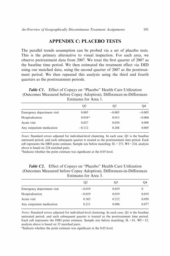
APPENDIX C: PLACEBO TESTS

The parallel trends assumption can be probed via a set of placebo tests.

This is the primary alternative to visual inspection. For each area, we

observe pretreatment data from 2007. We treat the first quarter of 2007 as

the baseline time period. We then estimated the treatment effect via DID

using our matched data, using the second quarter of 2007 as the posttreat-

ment period. We then repeated this analysis using the third and fourth

quarters as the posttreatment periods.

Table C1. Effect of Copays on “Placebo” Health Care Utilization(Outcomes Measured before Copay Adoption), Differences-in-Differences

Estimates for Area 1.

Q2 Q3 Q4

Emergency department visit 0.005 �0.005 �0.005

Hospitalization 0.018* 0.013 �0.004

Acute visit 0.027 0.054 0.098

Any outpatient medication �0.112 0.268 0.005

Notes: Standard errors adjusted for individual-level clustering. In each case, Q1 is the baseline

untreated period, and each subsequent quarter is treated as the posttreatment time period. Each

cell represents the DID point estimate. Sample size before matching: IL=273, WI=224, analysis

above is based on 224 matched pairs.

*Indicate whether the point estimate was significant at the 0.05 level.

Table C2. Effect of Copays on “Placebo” Health Care Utilization(Outcomes Measured before Copay Adoption), Differences-in-Differences

Estimates for Area 3.

Q2 Q3 Q4

Emergency department visit �0.019 0.019 0

Hospitalization �0.019 0.019 0.019

Acute visit 0.365 0.212 0.058

Any outpatient medication 0.211 0.096 0.077

Notes: Standard errors adjusted for individual-level clustering. In each case, Q1 is the baseline

untreated period, and each subsequent quarter is treated as the posttreatment time period.

Each cell represents the DID point estimate. Sample size before matching: IL=81, WI=52,

analysis above is based on 52 matched pairs.

*Indicate whether the point estimate was significant at the 0.05 level.


APPENDIX D: ADDITIONAL OUTCOME RESULTS

In the main text, we report DID estimates. Here, we report the estimated

treated-control mean differences for outcomes in the posttreatment period.

We also include the full results for medication usage by type of medication.

Table D2. Effect of Copays on Health Care Utilization: MeanDifferences, 2008�2010 Medications by Type, Area 1.


Preventive medications 0.03 0.01 0.02 [�0.03, 0.07] 0.468

Acne medications 0.01 0.006 0.006 [�0.004, 0.01] 0.227

Allergy medications 0.04 0.02 0.01 [�0.009, 0.04] 0.191

Topical antibiotics 0.005 0.005 �0.0004 [�0.004, 0.003] 0.816

ADHD medications 0.15 0.02 0.13 [0.01, 0.24] 0.025

Antibiotics 0.06 0.06 �0.005 [�0.02, 0.01] 0.674

Eczema medications 0.01 0.01 0.0007 [�0.012, 0.014] 0.918

Gastrointestinal medications 0.009 0.004 0.005 [�0.003, 0.01] 0.253

Hypertension medications 0.008 0 0.008 [0.001, 0.01] 0.019

Neuro medications 0.01 0.002 0.01 [0.002, 0.023] 0.016

Pain medications 0.02 0.01 0.007 [�0.008, 0.02] 0.352

Psychiatric medications 0.04 0.01 0.03 [0.004, 0.06] 0.023

Reflux medications 0.009 0.005 0.003 [�0.004, 0.01] 0.406

Respiratory medications 0.06 0.04 0.01 [�0.03, 0.05] 0.544

Steroids 0.01 0.003 0.01 [�0.004, 0.02] 0.165

Optional medications 0.06 0.03 0.03 [�0.01, 0.07] 0.188



Table D1. Effect of Copays on Health Care Utilization: MeanDifferences, 2008�2010 Outcomes, Area 1.


Emergency department visit 0.38 0.41 �0.03 [�0.15, 0.09] 0.647

Hospitalization 0.02 0.06 �0.04 [�0.12, 0.03] 0.323

Acute visit 0.52 1.29 �0.77 [�1.04, �0.51] 0.000

Well child visit 0.38 0.47 �0.10 [�0.17, �0.02] 0.014

Any outpatient medication 0.58 0.28 0.29 [0.12, 0.46] 0.000




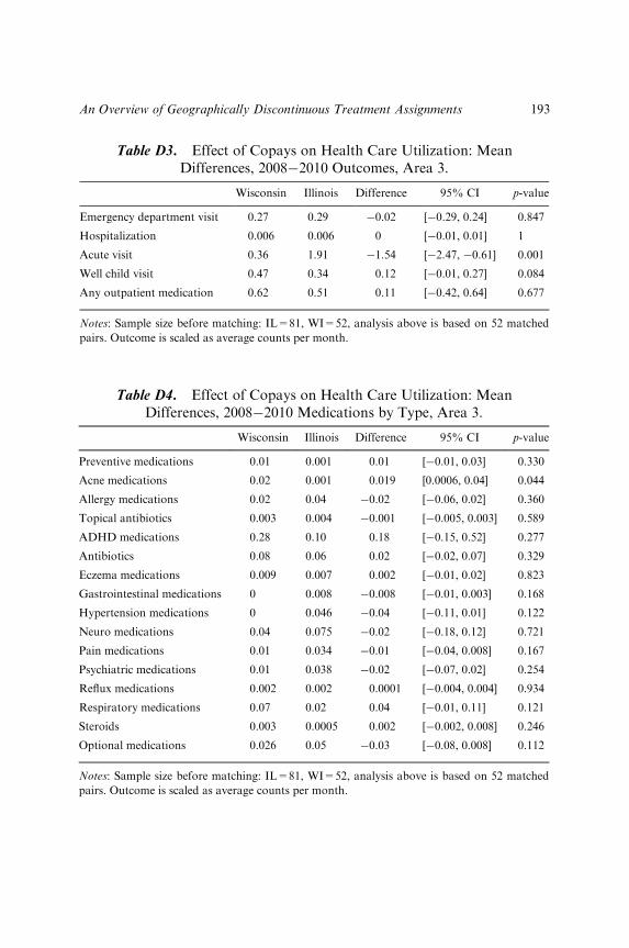
Table D3. Effect of Copays on Health Care Utilization: MeanDifferences, 2008�2010 Outcomes, Area 3.


Emergency department visit 0.27 0.29 �0.02 [�0.29, 0.24] 0.847

Hospitalization 0.006 0.006 0 [�0.01, 0.01] 1

Acute visit 0.36 1.91 �1.54 [�2.47, �0.61] 0.001

Well child visit 0.47 0.34 0.12 [�0.01, 0.27] 0.084

Any outpatient medication 0.62 0.51 0.11 [�0.42, 0.64] 0.677

Notes: Sample size before matching: IL=81, WI=52, analysis above is based on 52 matched

pairs. Outcome is scaled as average counts per month.

Table D4. Effect of Copays on Health Care Utilization: MeanDifferences, 2008�2010 Medications by Type, Area 3.


Preventive medications 0.01 0.001 0.01 [�0.01, 0.03] 0.330

Acne medications 0.02 0.001 0.019 [0.0006, 0.04] 0.044

Allergy medications 0.02 0.04 �0.02 [�0.06, 0.02] 0.360

Topical antibiotics 0.003 0.004 �0.001 [�0.005, 0.003] 0.589

ADHD medications 0.28 0.10 0.18 [�0.15, 0.52] 0.277

Antibiotics 0.08 0.06 0.02 [�0.02, 0.07] 0.329

Eczema medications 0.009 0.007 0.002 [�0.01, 0.02] 0.823

Gastrointestinal medications 0 0.008 �0.008 [�0.01, 0.003] 0.168

Hypertension medications 0 0.046 �0.04 [�0.11, 0.01] 0.122

Neuro medications 0.04 0.075 �0.02 [�0.18, 0.12] 0.721

Pain medications 0.01 0.034 �0.01 [�0.04, 0.008] 0.167

Psychiatric medications 0.01 0.038 �0.02 [�0.07, 0.02] 0.254

Reflux medications 0.002 0.002 0.0001 [�0.004, 0.004] 0.934

Respiratory medications 0.07 0.02 0.04 [�0.01, 0.11] 0.121

Steroids 0.003 0.0005 0.002 [�0.002, 0.008] 0.246

Optional medications 0.026 0.05 �0.03 [�0.08, 0.008] 0.112

Notes: Sample size before matching: IL=81, WI=52, analysis above is based on 52 matched

pairs. Outcome is scaled as average counts per month.


APPENDIX E: COUNTY LEVEL TAX RATES

In the 2006�2008 period, county-level tax rates were higher in the Illinois

counties in our sample than in the Wisconsin counties in our sample.

According to a report by the Tax Foundation (The Tax Foundation 2012),

property tax rates (calculated as median taxes paid as a percent of median

home value) were as follows in our three areas. Area 1: Lake County (IL)

2.19% and Kenosha County (WI) 1.93%; Area 2: McHenry county (IL)

2.09% and Walworth (WI) 1.68%; Area 3: Winnebago County (IL) 2.39%

and Rock County (WI) 1.96%.The highest difference occurs in Area 3, where Winnebago County (IL)

has a 2.39% rate and Rock County (WI) a 1.96% rate, a 0.43 percentage

point difference (in the 2006�2008 period). This means that a house that

sold for $100,000 in Wisconsin would pay roughly the same amount in

property tax as a house that sold for $82,000 in Illinois. Thus, if house

prices fully incorporated the different tax rates in these these two areas, we

would expect to observe lower house prices in Illinois than in Wisconsin in

equilibrium (assuming there is free mobility). This is what we observe when

we compare median prices in our County Comparison column in Areas 1

and 2 (Table 1), although the magnitude of most of the differences reported

for Areas 1 and 2 are too large to be explained solely by difference in tax

rates, which suggests that the imbalances likely reflect other, perhaps more

problematic, differences between the adjacent counties. In contrast, Area 3

is the only area where the Geographic Match column shows a treated-

control difference in house prices that is small, and the magnitude of the

negative differences in the other two columns are consistent with the

county-level property tax differences we report in this area; this reinforces

our decision to focus on Area 3.


an overview of geographically discontinuous …

Documents