0

An Ordered Probit Model of Live Performance

Attendance for 24 EU Countries

Martin Falk and Rahel Falk

Austrian Institute of Economic Research (WIFO)

revised: March 2011

Abstract:

Using EU-SILC data for 24 EU countries, we investigate the determinants of live performance

attendance (i.e. participation and frequency of participation). Ordered probit models with and

without random household effects are estimated for a sample of about 351,000 individuals for

the year 2006. We find that both households’ disposable income and level of education have a

strong and positive impact on the probability of live performance attendance. Pupils and

university students, individuals in highly densely populated areas and, to a lesser extent, women

and part-time workers have a higher probability of attending live performances, while

particularly older and disabled people and, to lesser extent, pensioners, unemployed, people

born in Non-EU countries and persons living in large households all are determinants with

lower probabilities. Finally, there are considerable cross-country differences with respect to the

role of age, gender and degree of urbanisation across EU countries. In contrast, the impact of

education and income does not vary much across countries.

JEL: C25, Z1, D12.

Keywords: ordered probit model, cultural participation, live performance attendance.

*Corresponding author: Martin Falk, WIFO, Arsenal Objekt 20, A-1030 Vienna, Austria; phone: + 43-1-798 26 01 – 226, fax: + 43-1-798 93 86, e-mail: Martin.Falk@wifo.ac.at. Financial support from the European Commission within the framework of the Competitiveness Report is gratefully acknowledged. We would like to thank two anonymous referees for their helpful comments on an earlier draft of the paper. We would also like to thank the participants of two workshops at the EC's Directorate-General for Enterprise and Industry for very helpful comments. Finally, we would like to thank Tyler Schaffner and Noelle Crist-See for excellent proofreading.

1

1 Introduction

Growing empirical literature is finding great disparities in cultural participation among different

socio-economic groups and is coming to a broad consensus on the main reasons behind them.

More specifically, better-educated individuals and those with higher income are more likely to

attend performing arts events (Baumol and Bowen, 1966; Borgonovi, 2004; Gray, 2003).

Scholars generally agree that education is the most important predictor of participation in the

arts and their frequency (see Blaug, 2001; McCarthy, 2001; Seaman 2005, 2006 for surveys of

the literature). Other factors that make for differences in performing arts attendance relate to

age, gender, labour market status, urbanisation, and social status.

Descriptive evidence based on internationally comparable micro data show that participation in

live performances varies substantially across EU countries. The share of people that attend four

or more live performances every year ranges between 8 per cent or less in Italy, Greece and

Poland and 36 per cent in Austria, based on the survey of income and living conditions (SILC)

in the year 2006 (Table 1 in the data section). The Scandinavian countries, the Netherlands,

United Kingdom, Luxembourg and Estonia have higher-than-average attendance rates. Given

the large variation in live performance attendance across countries, it is natural to ask to whether

the cross-country differences remain when socio-economic characteristics such as education,

income and age are controlled for. Another interesting question is to what extent the

determinants of live performance attendance differ across countries and what the common

factors are.

The aim of this paper is to give new empirical insights into the patterns of live performance

attendance (e.g. in plays, concerts, operas, and ballet and other dance performances) in 24 EU

countries, based on internationally comparable individual and household data. We use the EU-

SILC database and the cultural and social participation module for 2006, which contains

information on whether or not people participated in live performances and the frequency of

such visits measured as categories. The data allow us to control for a number of observable

individual and household characteristics. The empirical model will be estimated using the

standard ordered probit model and the random effects ordered probit model accounting for

unobserved random household effects. The latter model is also often applied to ordinal data to

account either for clusters or for random individual effects (Rabe-Hesketh and Skrondal 2008).

This study contributes to the literature on cultural participation in a number of ways. To begin

with, we use comparable micro data on participation in live performances covering all EU

countries. This allows us to investigate cross-country differences and the common patterns in

the characteristics influencing live performance attendance. Previous studies based on nationally

2

representative surveys are mainly based on one country, and there are very few studies

including two or three countries. The results of these studies are difficult to compare across

countries because of differences with respect to the sampling procedure, the reference period,

the specification of participation measures, the coding of answer options, the inclusion of

control factors, et cetera (Schuster 1987; Kawashima 1995). Despite recent progress, there still

aren’t enough international comparisons on determinants of live performance attendance at the

micro level that are based on a large number of countries. To our knowledge, this is the first

micro-level study based on a large and representative body of data including a large number of

countries. From the standpoint of cultural policy, it is particularly interesting to observe the

extent to which countries are successful in evening out income and educational effects. To what

extent the determinants differ across countries is still an open question, and there are numerous

reasons why they do. For instance, education may play a less important role in countries that

already have a labour force with an above-average percentage of post-secondary education.

Furthermore, the income effect may be lower in countries with generous state subsidies to

cultural institutions, such as the Scandinavian and some other Western European countries. The

age effect may also differ across countries. In particular, the age effect may be lower in

countries where there are a large number of specific types of live performances – such as

theatre, opera, and classical music – that are especially popular among older people. Another

contribution of the paper refers to methodology. The structure of the data allows the control for

unobserved heterogeneity using household random effects. One might expect the inclusion of

household random effects to lead to results that area more reliable because the participation

behaviour within households is highly correlated.

The structure of the paper is as follows. Section 2 presents the previous literature. Section

introduces the empirical model and the hypotheses. In Section 4, we present some summary

statistics, and in section 5, the empirical results. Section 6 contains some concluding remarks.

2 Previous literature

There is an increasing number of studies on cultural participation that use discrete-choice

models applied to individual data. For a comprehensive review of more recent literature see

Seaman (2005, 2006) and Petit (2000). A common feature of these studies is that they are based

on representative national surveys. Previous micro level studies determining cultural

participation using discrete-choice models based on individual data can be divided into two

subgroups: one that focuses on the decision to participate, and one that investigates both the

initial participation decision and (if applicable) the frequency of such visits. Examples of the

3

first group include Favaro and Frateschi (2007) on attending musical performances in the

Netherlands, France, and Italy; Andreasen and Belk (1980) for theatre and symphony

attendance; and Hand (2009) for participation in music events. Examples of the second group

include Ateca-Amestoy (2008), Bihagen and Katz-Gerro (2000), Borgonovi (2004), Fisher and

Preece (2003), Lévy-Garboua and Montmarquette (1996), and Masters, Russell, and Brooks

(2011). With respect to the first group, most studies find that education and income are

significantly and positively related to the probability of arts attendance. In contrast, age is

significantly and negatively related to arts attendance, but depends on the type of art

performance (Favaro and Frateschi, 2007). Regarding the second group, the literature agrees

that education, income, age, gender, labour market status, household size, and degree of

urbanisation all play a significant role in determining cultural participation and the number of

such visits. For instance, Borgonovi (2004) investigates the decision to participate in particular

performing arts events and the level of attendance in such events using ordered logistics models.

The author finds that age, occupation, and educational background play an important role in the

frequency of attendance in opera, theatre, and ballet performances. Masters, Russell, and Brooks

(2011) investigate the determinants of attendance rates at art galleries, theatres, and ballet/opera

performances using ordered probit models. The authors find that gender, age, and education are

significant and show the expected sign. Using representative survey data for the United States in

2002, Ateca-Amestoy (2008) studies the determinants of theatre attendance by ascertaining

theatre participation (i.e. probability of never attending) and, when found, determining the

frequency of visits using zero-inflated count data models. The author finds that level of

education, income, age, residence in a metropolitan area, and in part, father’s level of education

are all significant determinants of the number of visits. Household size, however, is not

significant. The probability of never attending is lower for individuals with high incomes, single

people, women, and those who have received higher education.

3 Empirical model and hypothesis

The empirical literature on the determinants of cultural participation concludes that age, income

level, education, gender, leisure time, and degree of urbanisation all play an important role. In

the following analysis, we focus on live performance attendance because it is one of the key

variables among different cultural activities. The choice of the estimation technique is dictated

by the dependent variable. Live performance visits are measured by a number of categories of

4

an ordinal nature. Therefore, we use the ordered probit model (see Greene and Hensher, 2010).1

For each country the ordered probit model is specified as:

,11

*i

H

hhih

K

kkiki uXXY

)1,0(~ Nui ,

where i is the individual. Y takes five possible values: 0 for non-attendance, 1 for attendance of

“1-3” events, 2 for “4-6” events, 3 for “7-12” events, and 4 for “more than 12” instances of

attendance. The dependent variable is expressed as:

.4

3

2

1

0

*4

4*

3

3*

2

2*

1

1*

i

i

i

i

i

i

Yif

Yif

Yif

Yif

Yif

Y

41,.., are the unknown threshold parameters to be estimated. k and h are vectors of

coefficients; and ;iu is the error term, which is assumed to be normally and identically

distributed with mean zero and variance normalised to one. *iY is the latent response variable

ranging from to . kiX includes K variables of individual-specific characteristics (e.g.

gender, age, education, labour market status, and country of birth in non-EU countries). Labour

market status is defined as not in the labour force (i.e. part-time, unemployed, school-age or

university students, retired, permanently disabled, or the individual exhibits some other status).

hiX includes H variables indicating household characteristics, such as household size and

household income, and other properties, such as degree of urbanisation. The ordered response

model can be estimated by the standard ordered probit model or the ordered logit model using

maximum likelihood techniques. Since preliminary estimates show that the results of the two

models are fairly similar, we only report the results of the ordered probit model. The standard

errors are clustered by households, allowing the errors to be correlated across individuals within

the same household. The reason for this is that individuals in the same household may share

similar characteristics. Age and household income are measured as logarithms. We also test

alternative functional forms with or without logarithmic transformations and quadratic forms as

well as piecewise linear forms. However, preliminary estimates show that the quadratic terms of

the log transformed series are never significant, indicating that a linear functional form cannot

be rejected. The same holds true for piecewise linear forms. To give an idea of the magnitude of 1 For a previous application of the ordered probit model in this area, see Masters, Rusell, and Brooks (2011).

5

the estimated effects, we compute the marginal effects of the dummy variables that measure the

impact of the explanatory variables. In addition, we calculate the predicted probabilities for the

two continuous variables age and household income. Note that the marginal effects sum to zero

and the predicted probabilities sum to 1.

For most of the countries, there is information available that indicates when individuals belong

to the same household. Individuals living in the same household share some observed and

unobserved attributes, giving rise to intra-household correlations. Since doing so would violate

the independence assumption that ordinal regression models assume, ignoring this kind of intra-

correlation would lead to inconsistent estimates and misleading inferences. Therefore, we use

the ordered probit model with random household effects (see Rabe-Hesketh and Skrondal, 2008;

Winkelmann 2005; and Nagel, Damen and Haanstra, 2010 for previous applications of this

methodology). The ordered probit model with random household effects estimated for each

country separately is specified as:

,11

*ijj

H

hhijh

K

kkijkij uZXXY

)1,0(~ Nuij ,

where i is the individual and j denotes the household. The dependent and independent variables

are similar except for the inclusion of the household effects jZ . The ordered probit model with

random effects can be estimated using the gllamm command in stata 11.2 (Rabe-Hesketh and

Skrondal, 2008).

4 Data and descriptive results

The data used to estimate the characteristics of live performance attendance comes from the

cultural and social participation module of the EU-SILC survey, which was carried out in the

EU-27 countries plus Iceland and Norway in 2006 (EUROSTAT, 2010). The EU-SILC has

become the reference source on comparative statistics on income distribution, living conditions

and social exclusion in the EU (EUROSTAT, 2008). It contains information for a large number

of individual characteristics such as education, labour market status, country of birth, age,

citizenship, health status, occupation of employed persons and sectoral affiliation. It also

provides information on household characteristics.

The survey contains information on whether or not individuals participate in live art

performances, go to cinemas, visit cultural sites (e.g. archaeological sites, museums etc) and

attend live sport events, and the frequency of such visits are classified into four different

categories. In this analysis, we focus on the number of times the individual goes to live

6

performances (plays, concerts, operas, and ballet and other dance performances). Note that

cultural events can be performed either by professionals or by amateurs (EUROSTAT, 2010).

Information is available for five categories (none, “1-3”, “4-6”, “7-12”, and “13 or more” events

attended), and the reference period covers the last 12 months before the second quarter of the

survey year (2006).

Turning to the explanatory variables one of the key variables is the educational attainment level

reported which is based on ISCED (International Standard Classification of Education). We

construct two dummy variables: one for intermediate education (persons with a vocational

degree belonging to ISCED 3+4), and one for tertiary education including university and

doctoral degrees (ISCED 5+6); the reference category contains persons with no formal

qualification and primary education (ISCED 0-2). Labour market status is measured by a set of

dummy variables indicating whether persons are part-time employees, unemployed, school-age

or university students, retired, permanently disabled, or exhibit some other status, with full-time

work as the reference group. Country of birth is measured as a dummy variable that equals one

for persons born outside of the EU and zero otherwise. The degree of urbanisation of residence

is measured as two dummy variables - one for densely populated areas and the other for

intermediate areas. Rural areas represent the reference category. Eurostat distinguishes three

different types of regions based on population density and total population at the NUTS 5 level

(EUROSTAT, 2008). Densely populated areas are defined as areas with at least 50,000

inhabitants in a contiguous local area with more than 500 inhabitants per square kilometre.

Intermediate urbanized areas are defined as areas with a population density ranging between

100 and 499 inhabitants per square kilometre and a population of at least 50,000 inhabitants.

Thinly populated areas are areas not belonging to either intermediate urbanized areas or densely

populated areas. Household size is measured as a set of dummy variables (i.e. household size =

2, 3, 4 or 5 or more household members), with single households as the reference group.

We select individuals aged 16 years or older. We do not include Bulgaria and Romania since

they joined the EU after the survey year 2006. For 19 out of 24 EU countries, there is

information available that indicates whether individuals belong to the same household. The final

sample for the analysis contains information on about 351,000 individuals in 24 EU countries

(the EU-15 countries, plus the EU-10 countries except for Malta).

Table 1 presents the percentage distribution of individual participation and frequency of

participation in live performances across countries for the year 2006. Based on weighted

percentages for the EU-15 countries, about 55 per cent of individuals do not attend live

performances (such as theatre, concerts, opera, or ballet or other dance performances) at least

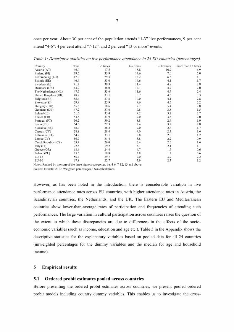
7

once per year. About 30 per cent of the population attends “1-3” live performances, 9 per cent

attend “4-6”, 4 per cent attend “7-12”, and 2 per cent “13 or more” events.

Table 1: Descriptive statistics on live performance attendance in 24 EU countries (percentages)

Country None 1-3 times 4-6 times 7-12 times more than 12 timesAustria (AT) 46.0 17.5 18.8 10.9 6.9Finland (FI) 39.5 33.9 14.6 7.0 5.0Luxembourg (LU) 47.0 29.3 13.2 6.3 4.1Estonia (EE) 46.6 33.0 14.6 4.1 1.7Sweden (SE) 41.7 39.3 11.4 4.8 2.8Denmark (DK) 43.2 38.0 12.1 4.7 2.0The Netherlands (NL) 47.7 33.6 11.6 4.7 2.4United Kingdom (UK) 48.2 33.1 10.7 4.6 3.3Belgium (BE) 55.4 27.8 10.0 4.1 2.8Slovenia (SI) 59.9 23.9 9.6 4.5 2.2Hungary (HU) 65.6 18.6 7.7 5.4 2.8Germany (DE) 47.2 37.6 9.8 3.8 1.5Ireland (IE) 51.5 33.4 9.2 3.2 2.7France (FR) 53.5 31.9 9.0 3.5 2.0Portugal (PT) 56.2 30.2 8.8 2.9 1.9Spain (ES) 64.3 22.3 7.4 3.2 2.8Slovakia (SK) 48.4 38.2 9.0 2.6 1.7Cyprus (CY) 58.8 28.4 9.0 2.3 1.6Lithuania (LT) 54.2 33.1 8.8 2.8 1.2Latvia (LV) 56.7 31.4 8.8 2.2 0.9Czech Republic (CZ) 63.4 26.0 6.4 2.6 1.6Italy (IT) 72.5 19.2 5.1 2.1 1.1Greece (GR) 68.6 24.4 4.7 1.7 0.6Poland (PL) 75.5 18.8 3.8 1.2 0.6EU-15 55.4 29.7 9.0 3.7 2.2EU-10 67.8 22.7 5.9 2.3 1.2

Notes: Ranked by the sum of the three highest categories, i.e. 4-6, 7-12, 13 and above.

Source: Eurostat 2010. Weighted percentages. Own calculations.

However, as has been noted in the introduction, there is considerable variation in live

performance attendance rates across EU countries, with higher attendance rates in Austria, the

Scandinavian countries, the Netherlands, and the UK. The Eastern EU and Mediterranean

countries show lower-than-average rates of participation and frequencies of attending such

performances. The large variation in cultural participation across countries raises the question of

the extent to which these discrepancies are due to differences in the effects of the socio-

economic variables (such as income, education and age etc.). Table 3 in the Appendix shows the

descriptive statistics for the explanatory variables based on pooled data for all 24 countries

(unweighted percentages for the dummy variables and the median for age and household

income).

5 Empirical results

5.1 Ordered probit estimates pooled across countries

Before presenting the ordered probit estimates across countries, we present pooled ordered

probit models including country dummy variables. This enables us to investigate the cross-

8

country variation in cultural participation when socio-economic characteristics are controlled

for. Table 4 in the Appendix shows the parameter estimates for the ordered probit models of live

performance attendance based on pooled data for 24 EU countries. The table contains the ß’s

and the z-values based on clustered standard errors, which are robust to correlation between

individuals within the same household. A positive and significant sign of the coefficients means

that individuals are significantly more likely to fall in the highest category “attendance 13 times

or more” (and significantly less likely to fall in the lowest attendance category “non-

attendance”) when the explanatory variable change. To better interpret the parameter estimates,

Table 3 in the Appendix also provides the marginal effects of the standard ordered probit

estimates. These estimates measure the effect of a unit change in each explanatory variable on

the probability of corresponding to one of the five categories of the dependent variable. The

marginal impact of each independent variable is calculated while holding constant all other

independent variables at their means.

The results of the standard ordered probit model show that household income, household size,

age, gender, education, country of birth in non-EU countries, and different types of labour

market status are all significant and show the expected sign. We find that the probability of live

performance attendance increases with household income and education for all four attendance

categories (“1-3”, “4-6”, “7-12” and “13 & more” times), while the category “no participation”

decreases with household income and education. Age has a negative effect on live performance

attendance, which indicates that the younger the person is, the more likely his or her attendance

at live performances and the higher the frequency thereof will be. Women have a significantly

higher probability of live performance attendance. People born in non-EU countries have a

higher probability of not attending a live performance at all and a lower probability of the

attending more than one. Turning to the effects of labour market status, we find that pensioners,

unemployed and people with disabilities exhibit lower probabilities of live performance

attendance and higher probabilities of non-attendance. In contrast, students and part-time

workers show significantly higher probabilities of attendance and lower probabilities of non-

attendance. This can be explained by the fact that students and part time workers have more

leisure time than other employees do. Household size has a negative effect on cultural

participation. This reflects the fact that the cost of attending a theatre or opera performance (on

a per-seat basis) rises quickly with the size of a household, and leaving dependents at home

often involves babysitting costs.

The marginal effects for level of education, age, income, and some labour market status

variables are quite large. For instance, the marginal effect for tertiary education shows that

9

being a college or university graduate reduces the probability of non-attendance by 32

percentage points compared with less qualified persons. The probability of attendance in the

four categories increases between 12 percentage points in the category “1-3” times and 4

percentage points in the category “13 and more” times. An increase in household income by 10

percent (from €20,000 to €22,000) will decrease the probability of non-attendance by 1.5

percentage points, and increase in the probability of live performance attendance of “1-3” times

by 0.8 percentage points. For the remaining three categories, “4-6”, “7-12” and “13 and more”

times, the increases in the probability are 0.4, 0.2 and 0.1 percentage points respectively.

Furthermore, an increase in age by 10 percent (equal to almost five years given the median age

of 47) increases the probability of non-attendance by 1.4 percentage points and reduces the

probability of attending at least one live performance by a value between 0.7 percentage points

the in the category “1-3” times and 1 percentage point in the category “13 and more”. The

marginal effects of students and disabled are also quite large, with a lower probability of non-

attendance of 22 percentage points and an increase in the probability of attendance in the four

categories ranging between 2 and 9 percentage points, depending on the answer category.

Disabled persons have a 16 percentage-point-higher probability of non-attendance.

The magnitude of the marginal effects of gender and some of the labour market status variables

(i.e. retired and unemployed people and part-time workers) is quite small. For instance, the

marginal effects for women show that being female reduces the probability of non-attendance

by 7 percentage points, whereas the probability of the frequency of attendance for the four

categories increase by 3, 2, 1 and zero percentage points. The marginal effects for people born

in non-EU countries have a range between 7 percentage points for the category “1-3 times” and

1 percentage point for the highest category “13 and more times”.

The country dummy variables show large and significant differences in live performance

attendance across EU countries after controlling for individual and household factors. We find

that the probability of live performance attendance (i.e. “1-3”, “4-6”, “7-12” and “13 and more”)

is highest in the Baltic States, followed by Austria, Portugal, Sweden and Finland. The other

East European countries (Slovakia, Czech Republic, and Slovenia, but not Poland) also exhibit

higher-than-average probabilities of attendance and lower probabilities of non-attendance. The

marginal effects of live performance attendance are lowest in some large European countries

(ES, FR, IT and PL). For United Kingdom and Germany, we find that the probability of

attendance is in the medium range. It is interesting to confront the cross-country variation in live

performance attendance with per capita government expenditures on arts performance. One

might expect the probability of live performance attendance to be higher in countries with high

10

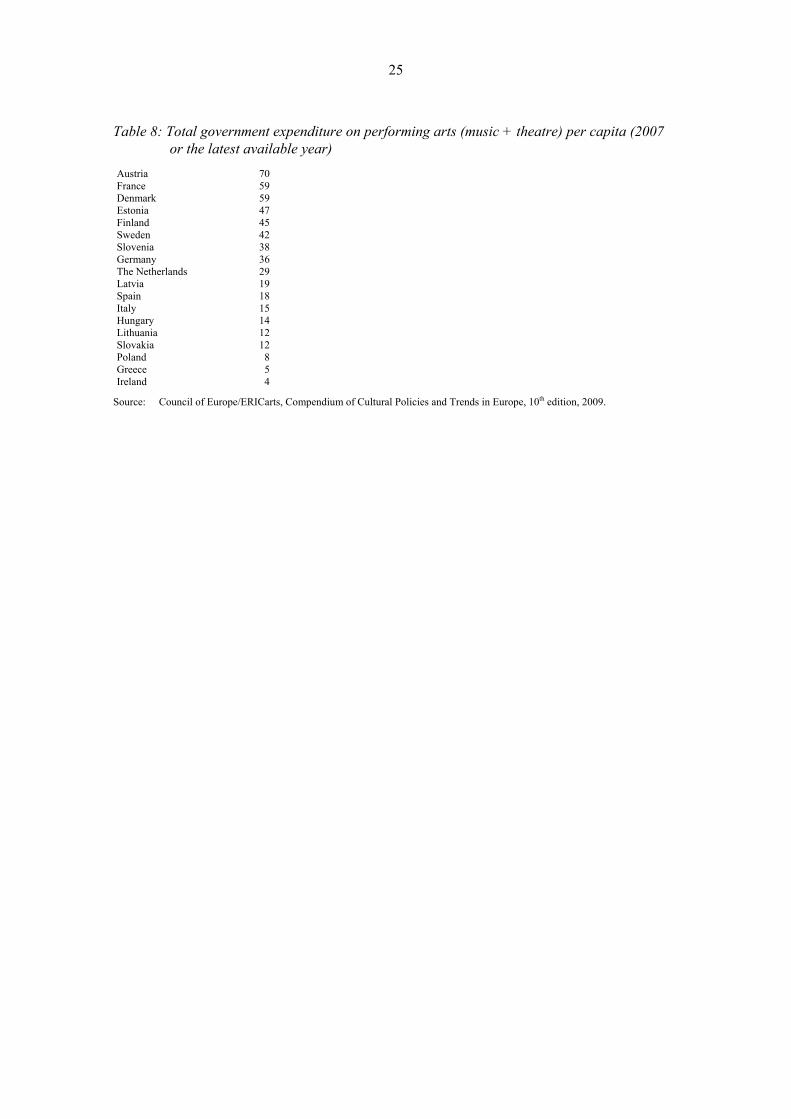
per capita government expenditures on arts performance. In fact, descriptive data show that per

capita government expenditures on arts performance are higher than average in Austria, Sweden

and Finland, based on the sample of countries for which data is available (see Table 8 in

appendix). Estonia and Slovenia also show a relatively high level of government expenditures

on performing arts per capita. Note that the rank of the two countries are even higher when

differences in purchasing power are taken into account. However, France and Germany,

countries that are also characterized by a high level of government expenditures on performing

arts, do not show the expected high probability of live performance attendance when for socio-

economic factors are controlled for. However, one should take into account that international

comparisons of government expenditures are problematic because of differences in the

definition and the problems of measuring indirect support for arts (Throsby, 1994).

5.2 Ordered probit estimates by country

Table 4 shows the results of the standard ordered probit model estimated separately for 24 EU

countries. Standard errors are robust to correlations within the household. Unreported results

show that the threshold parameters are statistically significant in all cases and show the expected

ordering. Tables 6 and 7 (in the Appendix) show the corresponding marginal effects of the

standard ordered probit model for each answer attendance category. Due to space limitations,

we report marginal effects for education, age, household income, gender and degree of

urbanisation.

As a robustness check we provide the results of the ordered probit model with random

household effects for all countries for which information on more than one household member

is available – excluding the Scandinavian countries, the Netherlands and Slovenia (see Table 5

in the Appendix). The estimated variance of the random household/family effect is significant in

all countries, indicating that unmeasured household attributes are, in fact, important. In the

following, the interpretation of the results focuses on the standard ordered probit model, since

household effects cannot be modelled for 5 out of 24 EU countries. When the estimates obtained

from the ordered probit model with random household effects are compared to those from the

standard ordered probit model, we find higher coefficients for income, education, gender, and

age in absolute terms for all countries (see Table 4 and Table 5 in the appendix). In contrast, the

coefficients for school-age and university students are much smaller and no longer significant in

some countries. Surprisingly, we find that the standard errors for the ordered probit model with

random household effects are lower than those obtained from the ordered probit model, ignoring

random household effects. Furthermore, unreported results reveal that the predicted probabilities

11

and the marginal effects for the key variables income, education and age do not differ much

between the standard ordered probit model and that accounting for random household effects.

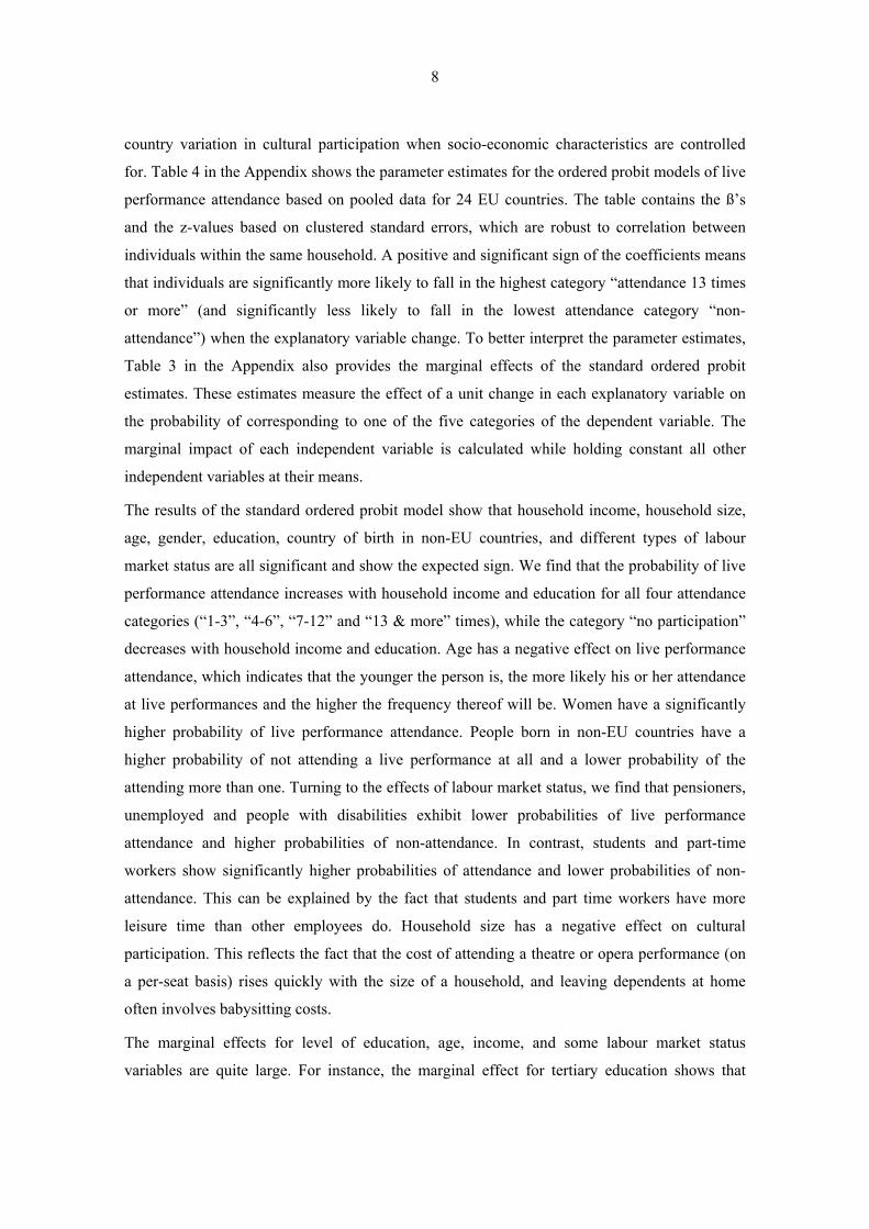
Table 2: Ordered probit model for live performance attendance by country

Log H‘hold

in-come

Log age

Fe-male

Non-EU

born

education Labour market status (ref. employed) Urbanisation Interme-diate

Ter-tiary

part-time

unem-ployed

pupil/stud.

retire-ment

disabled

other status

Den-sely

Inter-me-diate # of obs

AT 0.37 0.01 0.24 -0.85 0.52 0.94 0.09 -0.25 0.61 -0.14 -0.53 -0.12 0.09 0.05 11935(8.62) (0.13) (12.4) (-13.9) (18.4) (23.7) (2.65) (-3.54) (11.1) (-3.86) (-1.81) (-3.06) (2.58) (1.37)

BE 0.43 -0.12 0.10 -0.38 0.30 0.75 0.11 -0.09 0.52 -0.11 -0.23 -0.02 0.21 0.12 10495(11.8) (-2.32) (4.89) (-6.53) (9.62) (20.7) (2.83) (-1.78) (9.02) (-2.31) (-2.76) (-0.33) (2.82) (1.66)

CY 0.42 -0.48 0.22 -0.41 0.39 0.86 0.08 -0.15 0.48 -0.15 -0.57 0.01 -0.11 0.06 8601(12.0) (-9.04) (9.81) (-6.27) (10.6) (18.8) (1.17) (-1.67) (8.85) (-2.34) (-2.38) (0.26) (-2.81) (1.10)

CZ 0.49 -0.41 0.39 -0.34 0.46 1.17 0.00 -0.33 0.75 -0.10 -0.51 -0.47 0.14 0.10 14760(14.4) (-8.43) (21.9) (-2.20) (13.1) (24.2) (0.05) (-5.45) (13.9) (-2.26) (-7.53) (-8.90) (4.65) (3.01)

DE 0.42 0.04 0.25 -0.12 0.24 0.56 0.16 -0.41 0.53 0.14 -0.48 0.01 0.25 0.13 25450(20.6) (1.36) (18.2) (-4.23) (10.2) (21.3) (7.55) (-10.1) (14.3) (5.03) (-7.32) (0.38) (9.40) (4.78)

DK 0.33 -0.14 0.08 -0.40 0.31 0.55 -0.09 -0.19 0.26 -0.26 -0.53 -0.36 0.35 0.11 5549(7.55) (-2.26) (2.64) (-4.03) (7.90) (12.5) (-1.59) (-1.74) (3.78) (-4.52) (-5.70) (-2.87) (9.32) (3.09)

EE 0.42 -0.57 0.38 -0.48 0.44 1.04 0.11 -0.40 0.44 -0.42 -0.66 -0.38 -0.13 n.a 12945(15.6) (-13.3) (20.9) (-12.3) (14.8) (28.2) (1.82) (-6.39) (10.2) (-9.84) (-8.95) (-7.68) (-4.33)

ES 0.26 -0.40 0.11 -0.45 0.43 0.69 0.00 -0.08 0.42 -0.11 -0.37 -0.05 0.07 -0.01 26178(11.4) (-12.9) (7.46) (-8.80) (19.4) (29.6) (-0.09) (-2.34) (12.2) (-3.37) (-5.39) (-1.88) (2.78) (-0.23)

FI 0.29 -0.05 0.31 -0.39 0.29 0.70 0.12 -0.34 0.43 -0.13 -0.28 -0.30 0.41 0.27 10603(9.70) (-1.21) (14.1) (-3.03) (9.83) (22.0) (2.69) (-6.08) (8.47) (-3.12) (-5.05) (-5.19) (14.7) (8.97)

FR 0.43 -0.30 0.14 -0.24 0.33 0.79 0.10 -0.10 0.41 -0.09 -0.21 -0.08 0.14 0.08 18957(15.5) (-7.81) (9.52) (-5.96) (14.7) (27.6) (3.37) (-2.39) (9.76) (-2.67) (-4.06) (-1.95) (4.45) (2.54)

GR 0.35 -0.61 0.11 -0.61 0.45 0.91 0.06 -0.06 0.34 -0.23 -0.71 -0.15 0.05 0.09 12088(11.2) (-11.8) (5.03) (-8.28) (13.6) (21.5) (1.04) (-1.02) (5.92) (-4.93) (-4.13) (-3.57) (1.24) (1.69)

HU 0.47 -0.75 0.15 0.01 0.49 1.18 0.14 -0.20 0.75 -0.13 -0.30 -0.24 0.33 0.17 16395(16.7) (-16.1) (8.82) (0.15) (16.6) (30.2) (2.33) (-3.65) (16.0) (-3.09) (-5.61) (-5.24) (10.4) (4.62)

IE 0.39 -0.04 0.22 -0.25 0.45 0.76 -0.04 -0.30 0.21 -0.23 -0.52 -0.20 0.26 0.06 7503(10.2) (-0.74) (6.53) (-2.35) (11.9) (18.0) (-0.80) (-3.30) (2.36) (-4.28) (-6.04) (-4.06) (6.91) (1.48)

IT 0.33 -0.50 0.09 -0.38 0.45 0.81 -0.03 -0.11 0.32 -0.18 -0.62 -0.17 0.05 0.01 45497(19.2) (-19.1) (7.98) (-8.81) (27.7) (34.7) ( (-0.92) (-3.46) (11.5) (-7.59) (-7.54) (-7.82) (2.46) (0.64)

LT 0.42 -0.65 0.27 -0.24 0.40 0.98 -0.04 -0.17 0.60 -0.34 -0.38 -0.38 -0.09 n.a. 9947(13.0) (-11.0) (12.9) (-4.07) (10.5) (19.2) (-0.56) (-2.49) (9.81) (-6.67) (-5.43) (-5.22) (-2.67)

LU 0.54 0.08 0.12 -0.17 (0.32 0.65 0.17 -0.15 0.71 -0.05 -0.27 -0.02 -0.07 0.02 7707(10.7) (1.37) (4.24) (-2.71) (9.57) (14.6) (3.42) (-1.83) (10.9) (-1.00) (-2.90) (-0.39) (-1.56) (0.49)

LV 0.34 -0.56 0.32 -0.23 0.48 1.07 0.07 -0.22 0.53 -0.30 -0.69 -0.22 -0.31 n.a. 8967(11.0) (-10.9) (13.8) (-5.33) (12.6) (21.4) (0.97) (-3.36) (8.63) (-5.96) (-5.86) (-3.51) (-8.63)

NL 0.45 -0.13 0.11 -0.30 0.35 0.71 0.11 -0.15 0.31 -0.10 -0.60 -0.04 n.a. n.a. 8739(13.0) (-2.49) (3.71) (-4.49) (11.0) (19.8) (3.13) (-1.39) (4.70) (-1.89) (-6.87) (-0.90)

PL 0.43 -0.83 0.10 0.20 0.36 1.02 0.06 -0.08 0.68 -0.11 -0.26 -0.21 0.25 0.07 34771(20.2) (-24.0) (7.75) (1.75) (15.1) (30.6) (1.33) (-2.39) (20.0) (-3.29) (-6.08) (-5.36) (10.8) (2.30)

PT 0.29 -0.88 -0.08 -0.34 0.34 0.53 -0.01 -0.21 0.13 -0.19 -0.58 -0.13 -0.30 -0.15 8531(9.67) (-17.8) (-3.72) (-2.88) (8.46) (10.6) (-0.12) (-3.81) (2.56) (-3.75) (-4.03) (-2.58) (-6.89) (-3.48)

SE 0.25 -0.16 0.02 -0.50 0.24 0.61 0.06 -0.27 0.43 -0.01 -0.52 0.02 0.27 0.10 6362(4.88) (-3.07) (0.65) (-7.49) (6.02) (13.9) (1.59) (-3.07) (6.60) (-0.15) (-6.66) (0.12) (7.42) (2.52)

SI 0.52 -0.09 0.17 -0.19 0.43 1.05 -0.21 -0.07 0.60 -0.22 -0.71 -0.34 n.a. n.a. 9382(8.86) (-1.49) (6.78) (-3.89) (13.2) (19.3) (-1.86) (-1.13) (10.8) (-4.70) (-2.50) (-3.14)

SK 0.32 -0.63 0.23 0.09 0.32 0.82 -0.07 -0.27 0.51 -0.20 -0.35 -0.30 -0.09 -0.03 12576(10.3) (-13.8) (13.7) (0.50) (8.89) (16.9) (-1.01) (-5.76) (10.3) (-4.56) (-3.43) (-3.22) (-2.57) (-0.84)

UK 0.29 0.07 0.15 -0.31 0.45 0.73 0.07 -0.25 0.54 0.00 -0.49 -0.18 0.00 -0.02 16459(12.0) (1.93) (9.52) (-7.54) (16.8) (24.7) (2.67) (-3.07) (9.76) (-0.02) (-8.53) (-4.46) (0.06) (-0.42)

Notes: Z-values are in parentheses. The marginal effects are calculated using the estimation results of the standard ordered probit model with standard errors clustered by households. Dummy variables measuring the household size are included but not shown due to space limitations. Dummy variables measuring the degree of urbanisation are not included because this information is not available for Netherlands and Slovenia.

Tables 6 and 7 show the marginal effects of the standard ordered probit model for each answer

in the attendance category estimated separately for each country. Due to space limitations, we

report marginal effects for education, age, household income, gender and degree of

urbanisation. We find that individuals with a tertiary degree and an intermediate education have

12

a significantly higher propensity of live performance attendance; this holds true for all EU

countries. The marginal effects of the two education dummies are significant at the 1 per cent

level in all EU countries. As expected, the marginal effects are higher for persons with a tertiary

education than those with an intermediate education. This again holds true for all countries.

Furthermore, we find that an increase in household income leads to a decrease in non-

participation and to an increase in the different attendance categories in all countries. The

marginal effects are significant at the 1 per cent level in all EU countries. Furthermore, age has

a significant and negative effect on the probability of person’s attendance in live performances

in 17 out of 24 EU countries. In 22 out of 24 EU countries, we find that that the probability of

live performance attendance is significantly higher for woman than for men. Turning to the

effects of labour market status by country, we find that unemployed people have a significantly

lower probability of live performance attendance and a higher probability of non-attendance in

17 out of 24 EU countries. Students and pupils have a significantly higher probability of live

performance attendance and a lower probability of non-attendance in all of the 24 countries.

Pensioners have a significantly lower probability of live performance attendance in 20 out of 24

countries. The degree of urbanisation (i.e. living in a densely populated area) has a positive

influence on participation, indicating that cultural opportunities and preferences differ greatly

between rural and urban areas.

In order to give an idea of the magnitude of the continuous variables, we calculate the predicted

probabilities for age and income. Graph 1 and Graph 2 in the Appendix show the predicted

probabilities of being in each attendance category with respect to variations in household

income and age. based on the standard ordered probit model estimated separately for each

country and with predicted probabilities pooled across countries.2 The probability of never

attending live performances is lowest for the youngest age group (aged 16-24) and then rises

steadily with age. Those individuals with a household income of €50,000-60,000 have a

predicated probability of never attending live performances of 0.56, while the corresponding

probability for those with an income of €10,000-20,000 is 0.66. Furthermore, the results of the

predicted probabilities show that household income and education are roughly equally important

in determining live performance attendance. For instance, predicted probability of live

performance attendance in the categories “1-3” and “4-6” times for individuals with a very high

household income (€90,000-100,000) is 34 per cent and 13 per cent, respectively. For

individuals in the very low income (€10,000-20,000) bracket, the probability for the categories

“1-3“ and “4-6“ visits is 24 and 6 percent, respectively. The difference between the two income 2 Predicted probabilities have also been calculated for the ordered probit model with random effects. These are not shown here because they are almost similar to that of the standard probit model.

13

groups is, therefore, 10 per cent, and 7 per cent, respectively. For tertiary education, the

marginal effects in the categories “1-3” and “4-6” are 12 and 10 percentage points, respectively,

as reported in Table 3 (in the Appendix).

There are remarkable cross-country differences in the determinants of public participation in

live performance and frequency thereof (see Tables 6 and 7 in the Appendix)). In particular, the

effect of age, gender and degree of urbanisation varies greatly across EU countries when

measured as the coefficient of the variation of the marginal effects.3 Participating in a public

viewing of live performances and the corresponding frequency do not depend on age in Austria,

Germany, Ireland, Luxembourg, Slovenia, or the United Kingdom, but are significantly negative

in the remaining countries. The insignificant relationship between age and the probability of

attending live performances in some countries (e.g. Austria, Finland, Germany and United

Kingdom) may be related to the greater dominance of high arts versus low arts in some

countries. However, this is rather speculative, and further studies are necessary to investigate the

correlation of age to low versus high arts. Furthermore, attending live performances in the EU-

10 countries and the Mediterranean countries is much more age-dependent. The gender effect is

very high in the Czech Republic, the Baltic States, Finland, Germany, and Austria, but low in

Denmark and Sweden and very low in the Mediterranean countries. Urbanisation plays an

important role in the Scandinavian countries (Denmark, Sweden, and Finland), Hungary and

Ireland. In contrast, we find that individuals in densely populated areas in the Baltic States,

Slovakia and Portugal have a lower probability of attending at least one live performance. The

differences in the relationship between urbanisation and live performance attendance across EU

countries could be due not only to demand factors but also supply factors. These include the

different systems of cultural policies across countries ranging from state-driven systems to more

decentralized systems with a higher degree of financial autonomy of local authorities (Van der

Ploeg, 2006). In recent years, there has been a tendency in some EU countries to be more

financially autonomous (Van der Ploeg, 2006; Urrutiaguer, 2005). Therefore, the finding of no

rural/urban gap in live performance attendance might be related to the higher financial

autonomy of local authorities.

Furthermore, there are fewer cross-country differences in the effects of income and education on

live performance attendance. The income coefficient ranges between 0.25 for Sweden and 0.54

for Luxembourg. We find a low income coefficient for Germany, Ireland, the United Kingdom,

and Spain, and a higher-than-average income coefficient for the EU-10 countries. The low

magnitude of the relationship between income and cultural participation in some EU-15

3 The coefficient of variation is not shown here but is available upon request.

14

countries indicates that cultural consumers regard live performances as a necessity good rather

than a luxury good. The effect of tertiary education is also larger for the EU-10 countries than

for the EU-15 countries. This indicates that education plays a more important role in the group

of countries that already have a lower-than-average share of labour force with tertiary education.

The magnitude of the relationship between the probability of live performance attendance and

tertiary education based on the four frequency categories is lowest in the Scandinavian

countries, Germany, Portugal, Luxembourg and the Netherlands. This group of countries is

characterized by a higher-than-average share of tertiary education in the population (except

Portugal).

6 Conclusions and discussion

Using unique comparable micro level data on cultural participation for 24 EU countries, we

investigate the determinants of live performance attendance across countries. Ordered probit

models with and without unobserved household effects are estimated based on the EU-SILC

cultural and social participation module of 2006 with about 351,000 observations. In general,

the results are robust when random household effects are taken into account. We find that

income, age, gender, education, country of birth, and different types of labour market status all

play a significant role in participation and the frequency thereof. Specifically, attendance of

performing arts events increases with higher household income and education, particularly for

individuals with tertiary education and to lesser extent for people with a post-secondary degree.

On average, age is significantly negatively related to live performance attendance, but there are

large differences across countries. We find a lower probability of attendance for men, retired

and unemployed people and people born in non-EU countries. The marginal effects show that

the level of education, age, income, and some labour market status variables (e.g. students and

disabled) are most important in determining live performance attendance. Household income

and education are equally important in determining live performance attendance. Furthermore,

when we control for the socio-economic characteristics such as income, education and labour

market status, we find large differences in live performance attendance across countries. In

particular, attendance of performing arts events is highest in the Baltic States, other central

European countries, and Scandinavian countries (except Denmark) and lower in Southern

European countries, while the large EU countries are in the middle group. Overall, the

differences of cultural participation across EU countries are not surprising given that European

countries not only have different systems of cultural policies but are also characterized by

considerable differences in per capita government expenditures on performing arts.

15

Separate ordered probit estimates for each country show that the role of age and gender in live

performance attendance varies greatly across countries, whereas the impact of household

income and education does not vary much across EU countries. In particular, the negative

relationship between age and live performance attendance is much more pronounced in Eastern

EU countries (EU-10) than in the Western EU countries (EU-15). The effect of age within the

latter group is lower in absolute terms in countries with a high level of GDP per capita as well

as generous government expenditures on performing arts.

The findings on the characteristics of cultural participation are quite relevant from a policy point

of view. They can provide guidance for cultural policy makers who have little knowledge about

the dependence of live performance attendance on age, gender, income and education across

countries. Knowledge of the determinants of participation in live performance attendance is also

important for policy makers aiming to broaden participation in the arts, especially that of

disadvantaged groups such as poor, undereducated, disabled and older people. A clear

understanding of the determinants of cultural participation and attendance could help local and

national policy makers to develop actions in order to raise the demand for cultural activities.

These actions may include measures of cultural education and vouchers to sections of the

population (Van der Ploeg, 2006).

The finding that live performance attendance declines with age in the majority of countries is

important for cultural policy makers. An aging population will lead to lower attendance at live

performances. Therefore, in countries with a high age dependency of arts performance

attendance there is a need to attract older people to attend live performances, by adapting

marketing strategies or by providing vouchers for older people, for instance. The higher

attendance of women as compared to men in Eastern EU countries could be related to

differences in gender role attitudes across EU countries. Higher attendance rates of women in

some countries may reflect the fact that few other leisure activities for women are available.

However, the effect of education and income is lower in the EU-15 countries than in the EU-10

countries, indicating that the former group of countries is more successful in reducing the

disparities in cultural participation between poor and undereducated people on the one hand and

rich and skilled people on the other hand.

Finally, there are some areas of possible future research. It would be interesting to estimate the

determinants of live performance attendance for different types of cultural consumers. The

sociology literature distinguishes between different types of cultural consumers: omnivores,

univores, paucivores and non-consumers or inactives. These groups differ with respect to the

level of consumption and to the demand for different types of cultural forms (e.g. low cultural

16

forms, such as cinema, and high level forms, such as classical music and opera) (see Alderson,

Junisbai and Heacock, 2007). In general, univores and paucivores are characterized by lower

attendance rates, particularly for high cultural forms. The EU-SILC cultural participation

module contains information for some of these different cultural activities. In particular, it

provides information on cinema visits, visits to cultural sites and sport event attendance.

Modelling the cross-country heterogeneity in the characteristics of cinema and cultural site

visits is an important area of research left for future investigation.

A further interesting question is whether the determinants of cultural participation are similar

for the participation decision and the number of such visits measured in categories. Zero

attendance is the most common category in our case. Zero-inflated ordered probit models allow

non-attendance to be generated by two distinct processes. One part describes the decision not to

participate in cultural events (logit or probit part of the model) and the second part describes the

probability of the number of visits (measured in categories) given that the individual is

participating. This model would allow researchers to distinguish inactive non-consumers from

other types of cultural consumers. Furthermore, the national questionnaire of some EU countries

is more detailed with respect to the type of performance. In Austria, for example, there is a

distinction between theatre, dance, classical music, and popular music events. Future work is

needed to detect whether the characteristics of live performance attendance differ between low

and high arts.

17

References

Alderson, A. S., Junisbai A. & Heacock I. (2007). Social status and cultural consumption in the United States. Poetics, 35, 191-212.

Andreasen, A. R., & Belk, R. W. (1980). Predictors of attendance at performing arts. The Journal of Consumer Research, 7(2) 112–120.

Ateca-Amestoy, V. (2008). Determining heterogeneous behavior for theater attendance. Journal of Cultural Economics, 32, 127–151.

Baumol, W., & Bowen, W. (1966). Performing Arts – The economic dilemma. New York: Twentieth Century Fund, 1966,

Bihagen, E., & Katz-Gerro, T. (2000). Culture consumption in Sweden: The stability of gender differences. Poetics, 27(5-6), 327–349.

Blaug, M. (2001). Where are we now on cultural economics. Journal of Economic Surveys, 15(2), 123-143.

Borgonovi, F. (2004). Performing arts attendance: an economic approach. Applied Economics, 36(17), 1871–1885.

Eurostat (2008). Detailed guidelines of EU-SILC (EU-SILC 065 Description of target variables: Cross-sectional and Longitudinal). Luxembourg.

Eurostat (2010). EU-SILC 2006 module for social participation. Luxembourg.

Favaro, D., & Frateschi, C. (2007). A discrete choice model of consumption of cultural goods: the case of music. Journal of Cultural Economics, 31(3), 205–234.

Fisher, T. C. G., & Preece, S. B. (2003). Evolution, extinction, or status quo? Canadian performing arts audiences in the 1990s. Poetics, 31(2), 69–86.

Gray, C. M. (2003). Participation. In: Towse, R. (ed.), A Handbook of Cultural Economics, Edward Elgar, Cheltenham, 356–365.

Greene, W. H., & Hensher, D. A. (2010). Modeling Ordered Choices: A Primer and Recent Developments, Cambridge University Press 1–181.

Hand, C. (2009). Modelling patterns of attendance at performing arts events: the case of music in the United Kingdom. Creative Industries Journal 2(3), 259–271.

Kawashima, N. (1995). Comparing cultural policy: towards the development of comparative study. International Journal of Cultural Policy 1(2), 289–307.

Lévy-Garboua, L., & Montmarquette, C. (1996). A microeconomic study of theatre demand. Journal of Cultural Economics, 20(1), 25–50.

Masters, T., Russell, R., & Brooks, R. (2011). The demand for creative arts in regional Victoria, Australia. Applied Economics 43(5) 619-629.

McCarthy, K. F., Ondaatje, E. H., & Zakaras, L. (2001). Guide to the Literature on Participation in the Arts. Rand Corporation, Santa Monica, CA.

Nagel, I., Damen, M.-L., & Haanstra, F. (2010). The arts course CKV1 and cultural participation in the Netherlands. Poetics 38(4), 365–385.

Pettit, B. (2000). Resources for studying public participation in and attitudes towards the arts. Poetics, 27(5-6), 351–395.

Rabe-Hesketh, S. & Skrondal, A. (2008). Multilevel and Longitudinal Modeling using Stata. 2nd edition. College Station, TX: Stata Press.

Schuster, J. M. D. (1987). Making compromises to make comparisons in cross-national arts policy research. Journal of Cultural Economics 11(2), 1–36.

Seaman, B. A. (2005). Attendance and Public Participation in the Performing Arts: A review of the empirical literature, Working paper 05-03, Georgia State University.

Seaman, B. A. (2006). Empirical Studies of Demand for the Performing Arts, Handbook of the Economics of Art and Culture (Ch. 14), V.A. Ginsburgh & D. Throsby (ed.), North-Holland (Elsevier), 415-472.

Throsby, D. (1994). The production and Consumption of the Arts: A view of Cultural Economics. Journal of Economic Literature 31 (1) 1-29.

Urrutiaguer, D. (2005). French Decentralisation of the performing arts and regional economic disparities. Journal of Cultural Economics, 20(1), 299–312.

18

Van der Ploeg, Frederick (2006), The making of cultural policy: a European perspective. Handbook of the economics of Art and Culture. Ginsburgh V. A. And Throsby D. (eds), Vol 1. Amsterdam: Elsevier/North Holland, 1183-1221.

Winkelmann, R. (2005). Subjective well-being and the family: Results from an ordered probit model with multiple random effects, Empirical Economics, 30(3), 749–761.

19

Appendix:

Table 3: Descriptive statistics of the independent variables (means and percentages)

Median or percentages

disposable household income in € (median) 19867 age in years (median) 47 female 0.53 country of birth: non EU country 0.05Educational attainment: primary education (ISCED 0-2) (reference category) 0.36 intermediate education (ISCED 3+4 ) 0.45 rertiary education (ISCED 5+6) 0.19Labour market status: full time employee (reference category) 0.43 part time employee 0.08 unemployed 0.05 school-age and university students 0.08 retired persons 0.22 disabled 0.03 other status 0.10Household size: household size = 1 (reference category) 0.12 household size = 2 0.29 household size = 3 0.22 household size = 4 0.23 household size = 5 and more 0.14Degree of urbanisation densely populated areas 0.43 intermediate areas 0.29 rural areas (reference category) 0.28# of obs 350,529

Notes: EU SILC 2006 for EU 15 and EU-10 countries (excluding Malta). Unweighted percentages. Own calculations.

20

Table 4: Ordered probit model for live performances

Estimates Marginal effects in percentage points coef. z none 1-3 4-6 7-12 >=13

log disposable household income 0.38 *** 60.9 -0.15 0.08 0.04 0.02 0.01 log age -0.35 *** -40.9 0.14 -0.07 -0.04 -0.02 -0.01 female 0.17 *** 45.8 -0.07 0.03 0.02 0.01 0.00Educational attainment (ref. category: ISCED 0-2) intermediate education: (ISCED 3+4) 0.38 *** 67.9 -0.15 0.08 0.04 0.02 0.01 tertiary education (ISCED 5+6) 0.81 *** 115.0 -0.32 0.12 0.10 0.06 0.04 country of birth: non EU country -0.32 *** -28.4 0.12 -0.07 -0.03 -0.01 -0.01Labour market status (reference category: full time) part time employee 0.05 *** 6.0 -0.02 0.01 0.01 0.00 0.00 unemployed -0.17 *** -15.5 0.06 -0.04 -0.02 -0.01 0.00 school-age and university students 0.55 *** 57.4 -0.22 0.09 0.07 0.04 0.02 retired persons -0.11 *** -14.3 0.04 -0.02 -0.01 -0.01 0.00 disabled -0.43 *** -28.9 0.16 -0.09 -0.04 -0.01 -0.01 other status -0.14 *** -16.3 0.05 -0.03 -0.01 -0.01 0.00 household size =2 (reference category: 1) -0.23 *** -26.4 0.09 -0.05 -0.02 -0.01 -0.01 household size =3 -0.45 *** -44.6 0.17 -0.10 -0.04 -0.02 -0.01 household size =4 -0.49 *** -45.3 0.18 -0.10 -0.05 -0.02 -0.01 household size =5 and more -0.62 *** -50.4 0.22 -0.13 -0.06 -0.02 -0.01Country dummy variables (ref. cat: Germany, DE) Austria (AT) 0.40 *** 23.3 -0.16 0.07 0.05 0.03 0.02 Belgium (BE) -0.14 *** -8.0 0.05 -0.03 -0.01 -0.01 0.00 Cyprus (CY) -0.21 *** -11.5 0.08 -0.05 -0.02 -0.01 0.00 Czech Republic (CZ) 0.08 *** 4.3 -0.03 0.02 0.01 0.00 0.00 Denmark (DK) -0.07 *** -4.3 0.03 -0.02 -0.01 0.00 0.00 Estonia (EE) 0.61 *** 34.9 -0.24 0.09 0.08 0.04 0.03 Spain (ES) -0.05 *** -3.6 0.02 -0.01 -0.01 0.00 0.00 Finland (FI) 0.22 *** 16.2 -0.09 0.04 0.03 0.01 0.01 France (FR) -0.08 *** -5.9 0.03 -0.02 -0.01 0.00 0.00 Greece (GR) -0.29 *** -15.8 0.11 -0.06 -0.03 -0.01 -0.01 Hungary (HU) 0.23 *** 12.3 -0.09 0.04 0.03 0.01 0.01 Ireland (IE) -0.09 *** -5.2 0.03 -0.02 -0.01 0.00 0.00 Italy (IT) -0.39 *** -32.3 0.14 -0.09 -0.04 -0.01 -0.01 Lithuania (LT) 0.51 *** 25.7 -0.20 0.08 0.07 0.03 0.02 Luxembourg (LU) -0.06 *** -3.1 0.02 -0.01 -0.01 0.00 0.00 Latvia (LV) 0.48 *** 22.9 -0.19 0.08 0.06 0.03 0.02 Netherlands (NL) 0.03 ** 2.3 -0.01 0.01 0.00 0.00 0.00 Poland (PL) -0.18 *** -11.3 0.07 -0.04 -0.02 -0.01 0.00 Portugal (PT) 0.39 *** 20.1 -0.15 0.07 0.05 0.02 0.01 Sweden (SE) 0.09 *** 5.9 -0.04 0.02 0.01 0.00 0.00 Slovenia (SI) 0.07 *** 4.5 -0.03 0.01 0.01 0.00 0.00 Slovakia (SK) 0.49 *** 26.6 -0.19 0.08 0.06 0.03 0.02 United Kingdom (UK) 0.00 0.1 0.00 0.00 0.00 0.00 0.00 threshold parameter 1 2.62 ***

threshold parameter 2 3.63 ***

threshold parameter 3 4.23 ***

threshold parameter 4 4.74 ***

# of obs 350592Pseudo R2 0.11

Notes: ***, ** and * denote significance at the 1, 5, 10 level. The marginal effects are calculated using the estimation results of the standard ordered probit model with standard errors clustered by households. Dummy variables measuring the household size and the threshold parameters are not shown due to space limitations. Dummy variables measuring the degree of urbanisation are not included because this information is not available for Netherlands and Slovenia.

21

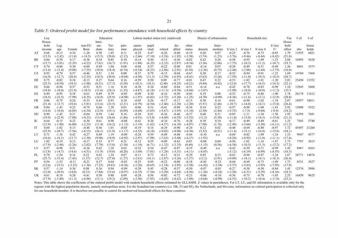
Table 5: Ordered probit model for live performance attendance with household effects by country

Log

Log age Female

non-EU Born

Education Labour market status (ref. employed) Degree of urbanisation Household size Var # of # of House-

hold income

Inter-me-diate

Ter-tiary

part- time

unem-ployed

pupil/stud. retired

dis-abled

other status densely

Inter-mediate h’size 2 h’size 3 h’size 4

h’size 5+

Household effect obs

households

AT 0.68 -0.13 0.34 -1.20 0.58 1.03 0.11 -0.25 0.47 -0.26 -0.60 -0.19 0.20 0.07 -0.25 -0.76 -0.73 -0.85 1.79 11935 6021 (15.5) (-2.42) (11.8) (-14.5) (15.5) (20.0) (2.12) (-2.66) (7.10) (-5.24) (-1.92) (-3.58) (3.74) (1.23) (-3.76) (-9.46) (-8.44) (-8.42) (21.8)

BE 0.86 -0.39 0.17 -0.38 0.34 0.85 0.10 -0.14 0.50 -0.15 -0.36 -0.02 0.42 0.26 -0.58 -0.95 -1.09 -1.25 2.04 10495 5628 (15.7) (-5.81) (5.35) (-4.22) (7.61) (16.7) (1.91) (-1.88) (6.35) (-2.32) (-2.87) (-0.34) (3.36) (2.06) (-7.75) (-10.3) (-11.2) (-10.7) (19.7)

CY 0.74 -0.86 0.30 -0.60 0.49 1.04 0.06 -0.04 0.57 -0.22 -0.80 0.01 -0.14 0.07 -0.28 -0.49 -0.31 -0.49 1.26 8601 3575 (13.6) (-13.4) (9.08) (-7.55) (10.8) (18.4) (0.74) (-0.34) (8.23) (-2.86) (-2.91) (0.10) (-2.36) (0.75) (-2.44) (-3.88) (-2.44) (-3.75) (16.0)

CZ 0.93 -0.79 0.57 -0.46 0.51 1.34 0.00 -0.37 0.79 -0.15 -0.68 -0.67 0.28 0.17 -0.52 -0.94 -0.91 -1.23 1.69 14760 7468 (16.9) (-12.7) (20.4) (-2.35) (10.5) (20.0) (-0.04) (-4.50) (11.3) (-2.59) (-6.93) (-8.41) (5.63) (3.26) (-7.59) (-11.0) (-10.3) (-10.5) (20.7)

DE 0.75 -0.02 0.38 -0.13 0.27 0.64 0.16 -0.59 0.50 0.09 -0.77 -0.01 0.47 0.22 -0.53 -1.02 -1.01 -1.20 2.03 25450 13552 (25.5) (-0.54) (18.5) (-3.08) (8.31) (17.3) (5.58) (-10.1) (10.1) (2.48) (-8.25) (-0.21) (9.84) (4.42) (-12.0) (-17.7) (-16.5) (-14.3) (32.1)

EE 0.66 -0.94 0.57 -0.52 0.51 1.16 0.10 -0.38 0.34 -0.60 -0.84 -0.51 -0.14 n.a -0.42 -0.78 -0.83 -0.99 1.18 12945 5608 (18.8) (-18.0) (21.9) (-10.5) (13.6) (24.3) (1.35) (-4.87) (6.18) (-11.3) (-9.58) (-8.04) (-3.07) (-5.99) (-10.0) (-10.0) (-11.2) (15.5

ES 0.49 -0.95 0.18 -0.61 0.49 0.79 -0.05 -0.09 0.30 -0.16 -0.50 -0.05 0.18 0.00 -0.52 -0.75 -0.86 -1.00 1.74 26178 11612 (18.5) (-23.5) (7.99) (-8.35) (16.9) (25.9) (-0.98) (-1.97) (6.82) (-3.72) (-5.20) (-1.25) (4.70) (-0.09) (-8.36) (-11.6) (-13.1) (-12.9) (28.8)

FR 0.86 -0.75 0.24 -0.33 0.43 0.93 0.10 -0.05 0.26 -0.17 -0.17 -0.13 0.30 0.14 -0.61 -0.98 -1.02 -1.34 2.07 18957 10011 (21.4) (-13.7) (10.4) (-5.81) (13.6) (23.5) (2.21) (-0.79) (4.54) (-3.46) (-2.20) (-2.20) (5.51) (2.46) (-10.7) (-14.0) (-14.1) (-15.8) (26.4)

GR 0.84 -1.43 0.23 -0.79 0.66 1.28 0.01 -0.06 0.31 -0.41 -0.98 -0.34 0.18 0.25 -0.57 -0.88 -1.08 -1.43 2.92 12088 5522 (14.6) (-18.0) (6.05) (-6.34) (12.9) (19.1) (0.09) (-0.68) (3.65) (-5.67) (-3.93) (-5.10) (2.50) (2.44) (-5.33) (-7.5) (-9.04) (-9.9) (18.2)

HU 0.90 -1.42 0.21 -0.04 0.59 1.44 0.16 -0.38 0.81 -0.26 -0.46 -0.37 0.60 0.31 -0.85 -1.11 -1.30 -1.56 1.92 16395 7681 (19.9) (-22.9) (7.88) (-0.33) (13.9) (26.0) (1.86) (-4.91) (13.0) (-4.49) (-6.55) (-5.52) (11.2) (5.30) (-11.4) (-13.0) (-14.3) (-15.0) (21.3)

IE 0.64 -0.15 0.32 -0.30 0.61 0.98 -0.08 -0.41 0.20 -0.34 -0.76 -0.28 0.39 0.10 -0.17 -0.49 -0.49 -0.61 1.25 7503 5740 (12.9) (-1.90) (6.80) (-2.25) (11.4) (16.2) (-1.13) (-3.19) (1.62) (-4.57) (-6.10) (-4.07) (7.08) (1.76) (-2.49) (-5.64) (-5.30) (-6.11) (11.2)

IT 0.60 -1.02 0.13 -0.48 0.56 1.01 -0.05 -0.19 0.16 -0.29 -0.90 -0.24 0.12 0.02 -0.48 -0.69 -0.80 -0.97 1.72 45497 21260 (25.9) (-28.7) (7.56) (-8.13) (26.1) (31.9) (-1.17) (-4.52) (4.18) (-9.02) (-8.08) (-8.20) (3.52) (0.51) (-11.4) (-15.1) (-16.8) (-15.8) (34.1)

LT 0.71 -1.16 0.42 -0.27 0.49 1.19 -0.09 -0.24 0.59 -0.49 -0.48 -0.44 -0.10 n.a -0.69 -0.82 -1.09 -1.24 1.33 9947 4577 (16.6) (-16.1) (13.7) (-3.30) (9.98) (18.9) (-0.92) (-2.97) (7.98) (-7.63) (-5.48) (-4.37) (-1.93) (-8.26) (-8.92) (-11.0) (-11.1) (17.4)

LU 1.02 -0.19 0.13 -0.17 0.35 0.77 0.21 -0.12 0.55 -0.09 -0.43 0.03 -0.08 0.04 -0.56 -1.01 -1.16 -1.47 1.73 7707 3815 (17.9) (-2.48) (3.26) (-2.02) (7.79) (13.8) (3.10) (-1.10) (6.71) (-1.32) (-3.35) (0.44) (-1.15) (0.56) (-6.54) (-10.5) (-11.3) (-12.2) (17.2)

LV 0.57 -0.98 0.51 -0.26 0.62 1.28 0.02 -0.32 0.54 -0.47 -0.97 -0.35 -0.49 n.a -0.43 -0.59 -0.71 -0.99 1.45 8967 4263 (13.8) (-14.7) (14.6) (-4.51) (11.9) (19.0) (0.26) (-3.69) (7.01) (-7.28) (-5.31) (-4.11) (-8.85) (-5.12) (-6.19) (-6.99) (-8.55) (16.3)

PL 0.79 -1.54 0.16 0.22 0.43 1.24 0.07 -0.11 0.73 -0.13 -0.31 -0.29 0.45 0.15 -0.63 -0.94 -0.97 -1.34 1.67 34771 14876 (25.7) (-33.4) (7.45) (1.37) (12.7) (27.0) (1.27) (-2.61) (16.1) (-2.87) (-5.26) (-5.27) (12.2) (2.91) (-9.89) (-14.1) (-14.1) (-18.3) (26.4)

PT 0.54 -1.53 -0.11 -0.21 0.37 0.64 -0.03 -0.25 0.05 -0.22 -0.80 -0.18 -0.45 -0.23 -0.64 -0.69 -0.73 -1.09 1.73 8531 3827 (12.6) (-23.5) (-3.32) (-1.36) (7.23) (9.63) (-0.36) (-3.26) (0.65) (-3.18) (-3.95) (-2.58) (-6.43) (-3.38) (-5.57) (-5.83) (-5.95) (-7.95) (17.9)

SK 0.57 -1.14 0.36 0.08 0.36 0.94 -0.09 -0.38 0.45 -0.28 -0.57 -0.50 -0.07 -0.01 -0.27 -0.58 -0.50 -0.84 1.45 12576 5096 (12.0) (-20.9) (14.0) (0.31) (7.84) (15.6) (-0.97) (-6.35) (7.54) (-5.20) (-4.64) (-4.56) (-1.26) (-0.24) (-3.20) (-6.31) (-5.29) (-8.16) (24.3)

UK 0.61 -0.18 0.28 -0.41 0.50 0.80 0.09 -0.28 0.56 -0.02 -0.72 -0.23 -0.06 -0.10 -0.36 -0.73 -0.78 -1.05 2.25 16459 9625 (17.9) (-3.49) (11.3) (-6.98) (13.1) (19.2) (2.09) (-2.50) (7.85) (-0.45) (-8.62) (-3.89) (-0.68) (-0.99) (-6.52) (-10.2) (-10.4) (-11.0) (25.2)

Notes: This table shows the coefficients of the ordered probit model with random household effects estimated by GLLAMM. Z values in parentheses. For LT, LU, and EE information is available only for the regions with the highest population density, namely metropolitan areas. For the Scandinavian countries (i.e. DK, FI and SE), the Netherlands, and Slovenia, information on cultural participation is collected only for one household member. It is therefore not possible to control for unobserved household effects for these countries.

22

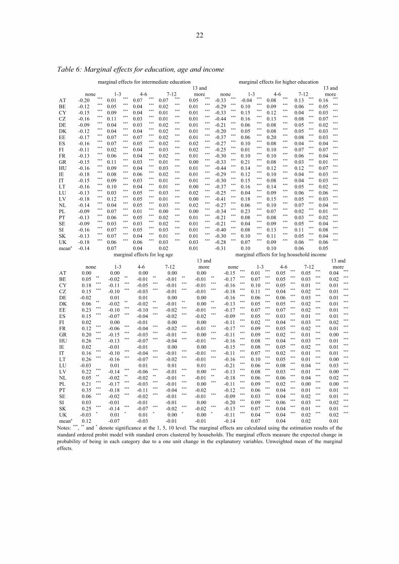
Table 6: Marginal effects for education, age and income

marginal effects for intermediate education marginal effects for higher education

none 1-3 4-6 7-12 13 and more none 1-3 4-6 7-12

13 and more

AT -0.20 *** 0.01 *** 0.07 *** 0.07 *** 0.05 *** -0.33 *** -0.04 *** 0.08 *** 0.13 *** 0.16 ***

BE -0.12 *** 0.05 *** 0.04 *** 0.02 *** 0.01 *** -0.29 *** 0.10 *** 0.09 *** 0.06 *** 0.05 ***

CY -0.15 *** 0.09 *** 0.04 *** 0.01 *** 0.01 *** -0.33 *** 0.15 *** 0.12 *** 0.04 *** 0.03 ***

CZ -0.16 *** 0.11 *** 0.03 *** 0.01 *** 0.01 *** -0.44 *** 0.16 *** 0.13 *** 0.08 *** 0.07 ***

DE -0.09 *** 0.04 *** 0.03 *** 0.02 *** 0.01 *** -0.21 *** 0.06 *** 0.08 *** 0.05 *** 0.02 ***

DK -0.12 *** 0.04 *** 0.04 *** 0.02 *** 0.01 *** -0.20 *** 0.05 *** 0.08 *** 0.05 *** 0.03 ***

EE -0.17 *** 0.07 *** 0.07 *** 0.02 *** 0.01 *** -0.37 *** 0.06 *** 0.20 *** 0.08 *** 0.03 ***

ES -0.16 *** 0.07 *** 0.05 *** 0.02 *** 0.02 *** -0.27 *** 0.10 *** 0.08 *** 0.04 *** 0.04 ***

FI -0.11 *** 0.02 *** 0.04 *** 0.03 *** 0.02 *** -0.25 *** 0.01 *** 0.10 *** 0.07 *** 0.07 ***

FR -0.13 *** 0.06 *** 0.04 *** 0.02 *** 0.01 *** -0.30 *** 0.10 *** 0.10 *** 0.06 *** 0.04 ***

GR -0.15 *** 0.11 *** 0.03 *** 0.01 *** 0.00 *** -0.33 *** 0.21 *** 0.08 *** 0.03 *** 0.01 ***

HU -0.16 *** 0.09 *** 0.04 *** 0.03 *** 0.01 *** -0.44 *** 0.14 *** 0.12 *** 0.12 *** 0.07 ***

IE -0.18 *** 0.08 *** 0.06 *** 0.02 *** 0.01 *** -0.29 *** 0.12 *** 0.10 *** 0.04 *** 0.03 ***

IT -0.15 *** 0.09 *** 0.03 *** 0.01 *** 0.01 *** -0.30 *** 0.15 *** 0.08 *** 0.04 *** 0.03 ***

LT -0.16 *** 0.10 *** 0.04 *** 0.01 *** 0.00 *** -0.37 *** 0.16 *** 0.14 *** 0.05 *** 0.02 ***

LU -0.13 *** 0.03 *** 0.05 *** 0.03 *** 0.02 *** -0.25 *** 0.04 *** 0.09 *** 0.06 *** 0.06 ***

LV -0.18 *** 0.12 *** 0.05 *** 0.01 *** 0.00 *** -0.41 *** 0.18 *** 0.15 *** 0.05 *** 0.03 ***

NL -0.14 *** 0.04 *** 0.05 *** 0.03 *** 0.02 *** -0.27 *** 0.06 *** 0.10 *** 0.07 *** 0.04 ***

PL -0.09 *** 0.07 *** 0.01 *** 0.00 *** 0.00 *** -0.34 *** 0.23 *** 0.07 *** 0.02 *** 0.01 ***

PT -0.13 *** 0.06 *** 0.05 *** 0.02 *** 0.01 *** -0.21 *** 0.08 *** 0.08 *** 0.03 *** 0.02 ***

SE -0.09 *** 0.03 *** 0.03 *** 0.02 *** 0.01 *** -0.21 *** 0.04 *** 0.09 *** 0.05 *** 0.04 ***

SI -0.16 *** 0.07 *** 0.05 *** 0.03 *** 0.01 *** -0.40 *** 0.08 *** 0.13 *** 0.11 *** 0.08 ***

SK -0.13 *** 0.07 *** 0.04 *** 0.01 *** 0.01 *** -0.30 *** 0.10 *** 0.11 *** 0.05 *** 0.04 ***

UK -0.18 *** 0.06 *** 0.06 *** 0.03 *** 0.03 *** -0.28 *** 0.07 *** 0.09 *** 0.06 *** 0.06 ***

meana -0.14 0.07 0.04 0.02 0.01 -0.31 0.10 0.10 0.06 0.05 marginal effects for log age marginal effects for log household income

none 1-3 4-6 7-12 13 and more none 1-3 4-6 7-12

13 and more

AT 0.00 0.00 0.00 0.00 0.00 -0.15 *** 0.01 *** 0.05 *** 0.05 *** 0.04 ***

BE 0.05 ** -0.02 ** -0.01 ** -0.01 ** -0.01 ** -0.17 *** 0.07 *** 0.05 *** 0.03 *** 0.02 ***

CY 0.18 *** -0.11 *** -0.05 *** -0.01 *** -0.01 *** -0.16 *** 0.10 *** 0.05 *** 0.01 *** 0.01 ***

CZ 0.15 *** -0.10 *** -0.03 *** -0.01 *** -0.01 *** -0.18 *** 0.11 *** 0.04 *** 0.02 *** 0.01 ***

DE -0.02 0.01 0.01 0.00 0.00 -0.16 *** 0.06 *** 0.06 *** 0.03 *** 0.01 ***

DK 0.06 ** -0.02 ** -0.02 ** -0.01 ** 0.00 ** -0.13 *** 0.05 *** 0.05 *** 0.02 *** 0.01 ***

EE 0.23 *** -0.10 *** -0.10 *** -0.02 *** -0.01 *** -0.17 *** 0.07 *** 0.07 *** 0.02 *** 0.01 ***

ES 0.15 *** -0.07 *** -0.04 *** -0.02 *** -0.02 *** -0.09 *** 0.05 *** 0.03 *** 0.01 *** 0.01 ***

FI 0.02 0.00 -0.01 0.00 0.00 -0.11 *** 0.02 *** 0.04 *** 0.03 *** 0.02 ***

FR 0.12 *** -0.06 *** -0.04 *** -0.02 *** -0.01 *** -0.17 *** 0.09 *** 0.05 *** 0.02 *** 0.01 ***

GR 0.20 *** -0.15 *** -0.03 *** -0.01 *** 0.00 *** -0.11 *** 0.09 *** 0.02 *** 0.01 *** 0.00 ***

HU 0.26 *** -0.13 *** -0.07 *** -0.04 *** -0.01 *** -0.16 *** 0.08 *** 0.04 *** 0.03 *** 0.01 ***

IE 0.02 -0.01 -0.01 0.00 0.00 -0.15 *** 0.08 *** 0.05 *** 0.02 *** 0.01 ***

IT 0.16 *** -0.10 *** -0.04 *** -0.01 *** -0.01 *** -0.11 *** 0.07 *** 0.02 *** 0.01 *** 0.01 ***

LT 0.26 *** -0.16 *** -0.07 *** -0.02 *** -0.01 *** -0.16 *** 0.10 *** 0.05 *** 0.01 *** 0.00 ***

LU -0.03 0.01 0.01 0.01 0.01 -0.21 *** 0.06 *** 0.08 *** 0.04 *** 0.03 ***

LV 0.22 *** -0.14 *** -0.06 *** -0.01 *** 0.00 *** -0.13 *** 0.08 *** 0.03 *** 0.01 *** 0.00 ***

NL 0.05 ** -0.02 ** -0.02 ** -0.01 ** -0.01 ** -0.18 *** 0.06 *** 0.06 *** 0.04 *** 0.02 ***

PL 0.21 *** -0.17 *** -0.03 *** -0.01 *** 0.00 *** -0.11 *** 0.09 *** 0.02 *** 0.00 *** 0.00 ***

PT 0.35 *** -0.18 *** -0.11 *** -0.04 *** -0.02 -0.12 *** 0.06 *** 0.04 *** 0.01 *** 0.01 ***

SE 0.06 *** -0.02 *** -0.02 *** -0.01 *** -0.01 *** -0.09 *** 0.03 *** 0.04 *** 0.02 *** 0.01 ***

SI 0.03 -0.01 -0.01 -0.01 0.00 -0.20 *** 0.09 *** 0.06 *** 0.03 *** 0.02 ***

SK 0.25 *** -0.14 *** -0.07 *** -0.02 *** -0.02 *** -0.13 *** 0.07 *** 0.04 *** 0.01 *** 0.01 ***

UK -0.03 * 0.01 * 0.01 * 0.00 * 0.00 * -0.11 *** 0.04 *** 0.04 *** 0.02 *** 0.02 ***

meana 0.12 -0.07 -0.03 -0.01 -0.01 -0.14 0.07 0.04 0.02 0.01Notes: ***, ** and * denote significance at the 1, 5, 10 level. The marginal effects are calculated using the estimation results of the standard ordered probit model with standard errors clustered by households. The marginal effects measure the expected change in probability of being in each category due to a one unit change in the explanatory variables. Unweighted mean of the marginal effects.

23

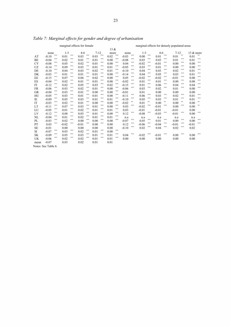
Table 7: Marginal effects for gender and degree of urbanisation

marginal effects for female marginal effects for densely populated areas

none 1-3 4-6 7-12 13 & more none 1-3 4-6 7-12 13 & more

AT -0.10 *** 0.01 *** 0.03 *** 0.03 *** 0.02 *** -0.03 *** 0.00 *** 0.01 *** 0.01 ** 0.01 **

BE -0.04 *** 0.02 *** 0.01 *** 0.01 *** 0.00 *** -0.08 *** 0.03 *** 0.03 *** 0.01 *** 0.01 ***

CY -0.08 *** 0.05 *** 0.02 *** 0.01 *** 0.00 *** 0.04 *** -0.02 *** -0.01 *** 0.00 *** 0.00 ***

CZ -0.14 *** 0.09 *** 0.03 *** 0.01 *** 0.01 *** -0.05 *** 0.03 *** 0.01 *** 0.00 *** 0.00 ***

DE -0.10 *** 0.04 *** 0.03 *** 0.02 *** 0.01 *** -0.10 *** 0.04 *** 0.03 *** 0.02 *** 0.01 ***

DK -0.03 *** 0.01 *** 0.01 *** 0.01 *** 0.00 *** -0.14 *** 0.04 *** 0.05 *** 0.03 *** 0.01 ***

EE -0.15 *** 0.07 *** 0.06 *** 0.02 *** 0.00 *** 0.05 *** -0.02 *** -0.02 *** -0.01 *** 0.00 ***

ES -0.04 *** 0.02 *** 0.01 *** 0.01 *** 0.00 *** -0.02 *** 0.01 *** 0.01 *** 0.00 *** 0.00 ***

FI -0.12 *** 0.02 *** 0.05 *** 0.03 *** 0.02 *** -0.15 *** 0.01 *** 0.06 *** 0.04 *** 0.04 ***

FR -0.06 *** 0.03 *** 0.02 *** 0.01 *** 0.00 *** -0.06 *** 0.03 *** 0.02 *** 0.01 *** 0.00 ***

GR -0.04 *** 0.03 *** 0.01 *** 0.00 *** 0.00 *** -0.01 0.01 0.00 0.00 0.00HU -0.05 *** 0.03 *** 0.01 *** 0.01 *** 0.00 *** -0.11 *** 0.06 *** 0.03 *** 0.02 *** 0.01 ***

IE -0.09 *** 0.05 *** 0.03 *** 0.01 *** 0.01 *** -0.10 *** 0.05 *** 0.03 *** 0.01 *** 0.01 ***

IT -0.03 *** 0.02 *** 0.01 *** 0.00 *** 0.00 *** -0.02 ** 0.01 ** 0.00 ** 0.00 ** 0.00 **

LT -0.11 *** 0.07 *** 0.03 *** 0.01 *** 0.00 *** 0.03 *** -0.02 *** -0.01 *** 0.00 *** 0.00 **

LU -0.05 *** 0.01 *** 0.02 *** 0.01 *** 0.01 *** 0.03 -0.01 -0.01 -0.01 0.00LV -0.12 *** 0.08 *** 0.03 *** 0.01 *** 0.00 *** 0.12 *** -0.08 *** -0.03 *** -0.01 *** 0.00 ***

NL -0.04 *** 0.01 *** 0.02 *** 0.01 *** 0.01 *** n.a n.a n.a n.a n.aPL -0.03 *** 0.02 *** 0.00 *** 0.00 *** 0.00 *** -0.07 *** 0.05 *** 0.01 *** 0.00 *** 0.00 ***

PT 0.03 *** -0.02 *** -0.01 *** 0.00 *** 0.00 0.12 *** -0.06 *** -0.04 *** -0.01 *** -0.01 ***

SE -0.01 0.00 0.00 0.00 0.00 -0.10 *** 0.02 *** 0.04 *** 0.02 *** 0.02SI -0.07 *** 0.03 *** 0.02 *** 0.01 *** 0.00 ***

SK -0.09 *** 0.05 *** 0.03 *** 0.01 *** 0.01 *** 0.04 *** -0.02 *** -0.01 *** 0.00 *** 0.00 ***

UK -0.06 *** 0.02 *** 0.02 *** 0.01 *** 0.01 *** 0.00 0.00 0.00 0.00 0.00mean -0.07 0.03 0.02 0.01 0.01

Notes: See Table 6.

24

Graph 1: Predicted probabilities of live performance attendance with respect to household income (pooled)

Graph 2: Predicted probabilities of live performance attendance with respect to age

Notes: The predicted probabilities are calculated using the standard ordered probit model based on 24 countries.

0.76

0.66

0.62 0.610.58

0.560.54

0.51

0.47

0.43

0.37

0.19

0.240.26 0.26 0.28

0.29 0.300.31

0.320.34 0.34

0.040.06

0.08 0.08 0.09 0.09 0.10 0.11 0.120.13

0.15

0.010.02 0.03 0.03 0.04 0.04 0.04 0.05 0.05 0.06

0.08

0.00 0.01 0.02 0.02 0.02 0.02 0.02 0.03 0.03 0.040.06

0.0

0.1

0.2

0.3

0.4

0.5

0.6

0.7

0.8

<10 10-20k 20-30k 30-40k 40-50k 50-60k 60-70k 70-80k 80-90k 90-100k >100k

pre

dic

ited

pro

bab

ilitie

s o

f liv

e p

erfo

rman

ces

bas

ed o

n th

e o

rder

ed

pro

bit

estim

ates

and

24

EU

co

untr

ies

none

1-3

4-6

7-12

13 and more

0.0

0.1

0.2

0.3

0.4

0.5

0.6

0.7

0.8

16 18 20 22 24 26 28 30 32 34 36 38 40 42 44 46 48 50 52 54 56 58 60 62 64 66 68 70 72 74 76 78 80

pre

dic

ted

pro

bab

ilitie

s o

f liv

e p

erfo

rman

ces

bas

ed o

n th

e o

rder

ed p

rob

it m

od

el a

nd 2

4 co

untr

ies

age in years

none

1-3

4-6

7-12

13 and more

25

Table 8: Total government expenditure on performing arts (music + theatre) per capita (2007 or the latest available year)

Austria 70 France 59 Denmark 59 Estonia 47 Finland 45 Sweden 42 Slovenia 38 Germany 36 The Netherlands 29 Latvia 19 Spain 18 Italy 15 Hungary 14 Lithuania 12 Slovakia 12 Poland 8 Greece 5 Ireland 4

Source: Council of Europe/ERICarts, Compendium of Cultural Policies and Trends in Europe, 10th edition, 2009.