an optimisation-based approach for process plant layout
TRANSCRIPT

AN OPTIMISATION-BASED APPROACH
FOR PROCESS PLANT LAYOUT
Jude O. Ejeh,† Songsong Liu,‡ Mazaher M. Chalchooghi,† and Lazaros G.
Papageorgiou∗,†
†Centre for Process Systems Engineering, Department of Chemical Engineering, University
College London, London WC1E 7JE, UK;
‡ School of Management, Swansea University, Bay Campus, Fabian Way, Swansea SA1
8EN, United Kingdom;
E-mail: [email protected]
Phone: +44 (0)20 7679 2563
Abstract
This paper presents an optimisation-based approach for the multi-�oor process plant
layout problem. The multi-�oor process plant layout problem involves determining
the most e�cient - based on prede�ned criteria - spatial arrangement of a set of pro-
cess plant equipment with associated connectivity. A number of cost and manage-
ment/engineering drivers (e.g. connectivity, operations, land area, safety, construction,
retro�t, maintenance, production organisation) have been considered over the last two
decades in order to achieve potential savings in the overall plant design process.
This work constitutes an extension of the previous work by Patsiatzis and Papageor-
giou 1 to address the multi-�oor process plant layout problem. New features introduced
modelled tall equipment with heights greater than the typical �oor height in chemical
process plants, with connection point at a design-speci�ed height for each equipment.
1

The number of �oors, land area, allocation of each equipment to a �oor and the over-
all layout of each �oor were determined by the optimisation model whilst preventing
overlap of equipment. The connection costs, horizontal and vertical, as well the con-
struction costs were accounted for with an overall objective to minimize the total cost.
The overall problem was formulated as a mixed-integer linear programming (MILP)
model based on a continuous domain representation and its applicability demonstrated
by a number of illustrative examples. Results showed an increase in the number of
equipment handled by the proposed models in modest computational times. Finally,
symmetry breaking constraints were included to increase computational e�ciency, and
their performance tested with the last example.
Keywords
Multi-�oor process plant layout; Mixed integer linear programming(MILP); Optimisation

1 INTRODUCTION 3
1 Introduction
Over the past two decades, the layout of equipment in process plants have gained increasing
relevance, from an economic, safety, operational and maintenance-related point of view.2,3
Layout design generally involves obtaining a suitable arrangement of items and their connec-
tions within a prede�ned area based on pre-speci�ed criteria. These items may be process
vessels and equipment, work centres or departments within an organisation; with connections
by pipes, conveyors, vehicular transport or any suitable material handling equipment.3,4
Layout designs have been found to have a tremendous impact on the costs and productivity
of any system involved2, as such researchers have constantly sought out methods to �nd the
best solution to such design problems - generally referred to as the layout problem. When
concerned with items that are needed for the production of goods or delivery of services, it
has been referred to as the facility layout problem.4 Amidst the classes of the facility layout
problem (see Drira et al. for a detailed review) is the process plant layout problem, on which
this work primarily focuses. Process plant layout problem addresses the layout problem for
items in a typical chemical process plant.5
Previous approaches to process plant layout design were from a practical point of view, where
decisions were made based on engineering judgement6, but especially from the late 90s,
more scienti�c approaches in terms of mathematical modelling have been adopted to solve
the problem1,7�12. Most of the previous research have focused on a cost-reducing objective,
with a varying number of scenarios. Georgiadis and Macchietto9 proposed a mathematical
programming approach with an objective to minimize cost - pumping, pipe connection and
�oor construction - and was formulated as a mixed integer linear programming (MILP) prob-
lem. Results showed the model was computationally e�cient for a small number of units.
Papageorgiou and Rotstein12 further solved the process plant layout problem over a continu-
ous spatial domain whilst introducing more realistic constraints for single-�oor case studies.
Barbosa-Povoa et al.7,8 accounted for di�erent inputs and outputs for each equipment, irreg-
ular shapes, a 3-dimensional representation, allowed for di�erent production sections, and

1 INTRODUCTION 4
safety and operability factors. These problems were all formulated as an MILP giving com-
putationally e�cient solutions for a small number of units.
Formulations to address scenarios with multiple �oors have also been considered. Patsiatzis
and Papageorgiou10 developed an MILP formulation to allow for a multi-�oor layout with
�oor construction costs (�xed and area-dependent) and vertical pumping costs. The model
successfully handled up to 11 units within a modest CPU time. For larger number of units,
Patsiatzis and Papageorgiou 1 proposed a rigorous decomposition approach and an iterative
solution scheme, with the later producing a solution with a higher degree of optimality. An
improvement-type algorithm was proposed by Xu and Papageorgiou13 applicable to a single
�oor.
Apart from a cost minimisation objective, other authors have introduced other criteria to the
objective function. Penteado and Ciric 5 presented a mixed integer non-linear programming
(MINLP) problem not only to minimize piping cost, land allocation cost, but also �nancial
risk and safety costs. Other factors have been the routing and layout of pipes6, safety and
risk assessment11,14�17, long-length equipment17�19, area minimisation20; with varying solu-
tion techniques17,21�25.
This paper proposes a generic model to the multi-�oor process plant layout problem, initially
proposed by Patsiatzis and Papageorgiou 1 (an improvement on Patsiatzis and Papageor-
giou 10) but extended to account for long-length equipment, i.e. equipment typically span-
ning multiple �oors, with connection points at design-speci�ed heights for each equipment.
Ku et al. 18 presented a MINLP model and accounted for tall equipment, minimizing total
layout area with a hybrid optimisation method. This work seeks to propose a more e�cient
MILP model to handle a larger number of units than previously recorded. Symmetry break-
ing constraints are also introduced to reduce solution search over multiple optimal solutions.
The rest of this paper is structured as follows: the problem is described in section 2 with
underlying assumptions; mathematical models are then proposed in section 3 to address the
problem; case studies to show model performance and applicability are presented in section

2 PROBLEM DESCRIPTION 5
4, where additional symmetry breaking constraints are also introduced and tested. Finally,
concluding remarks are given in section 5.
2 Problem Description
The following assumptions are made in the model formulation. Equipment items are de-
scribed by rectangular shapes. In all cases, rectilinear distances are assumed, with connec-
tions between equipment taken from their respective geometrical centres in the x-y plane.
Vertical distances are measured from a design-speci�ed height of each equipment. Each
equipment is allowed to rotate in 90o angles in the x-y plane, and must start from the base
of each available �oor. The �oor height is �xed across all �oors and if an equipment exceeds
such height, it is allowed to extend through available �oors.
The problem description for the process layout problem is as follows.
Given:
• a set of N equipment items and their dimensions (length, breadth and height);
• a set of K potential �oors for layout;
• connectivity network amongst equipment;
• cost data (connection, pumping, land, and construction);
• �oor height;
• space and equipment allocation limitations;
• minimum safety distances between equipment items;
determine:
• the total number of required �oors for the layout;
• the base land area occupied;

3 MATHEMATICAL FORMULATION 6
• the area of �oors;
• spatial equipment allocation to �oors;
so as to: minimise the total plant layout cost.
3 Mathematical Formulation
The mathematical formulation constitutes an extension to the work of Patsiatzis and Papageor-
giou 1. A full description of the model proposed by Patsiatzis and Papageorgiou 1 is available
in the supporting information. Two formulations (A & B) are proposed, primarily di�ering
in the manner tall equipment (which span multiple �oors) are handled. The �rst handles
multi-�oor equipment as is, by a set of constraints as summarised in Table 1 for each of the
three models proposed. The second formulation is a linearised form of the model proposed by
Ku et al. 18 (a direct extension of Patsiatzis and Papageorgiou 1), with multi-�oor equipment
divided into pseudo-single �oor units equivalent to the number of consecutive �oors they
require.
Table 1: Summary of equations adopted in models A.1 - A.3
ConstraintsFormulation A model
A.1 A.2 A.3Floor 1 - 4, 5 - 6 1 - 4, 5 - 6 1 - 4, 5 - 6Equipment orientation 9, 7 - 8 9, 7 - 8 9, 7 - 8Multi-�oor equipment 10-14 15 12, 13 and 16Distance 24,21, 22, 10, 12, 24 and 24,21, 22,
and 23 21, 22, 23, and 23Non-overlapping 17 - 20 17 - 20 17 - 20Area 31 - 36 31 - 36 31 - 36Layout design 30, 25 - 29 30, 25 - 29 30, 25 - 29

3 MATHEMATICAL FORMULATION 7
Nomenclature
Indices
i,j equipment item in models A.1 - A.3
i′,j′ equipment item in model B
k, k′ �oor number
p pseudo units
s rectangular area sizes
Sets
I set of equipment item for models A.1- A.3
I ′ set of equipment item for model B
MF set of multi-�oor equipments
Pi sets of pseudo units for equipment i
Parameters
αi, βi,γi dimensions of item i
Mi number of �oors required by item i
fij 1 if �ow direction between i and j is positive; 0, otherwise
OPij distance between the base and output point on equipment i
IPij distance between the base and input point on equipment j
BM a large number
FH �oor height
LC land cost
FC1 �xed �oor construction cost
FC2 area-dependent �oor construction cost
Ccij connection/piping costs

3 MATHEMATICAL FORMULATION 8
Chij horizontal pumping costs
Cvij vertical pumping costs
Integer variables
NF number of �oors required for layout
Binary variables
Oi 1 if length of item i is equal to αi; 0, otherwise
Wk 1 if �oor k is occupied; 0, otherwise
nijk 1 if items i and j are assigned to �oor k; 0, otherwise
Nij 1 if items i and j are assigned to the same �oor; 0, otherwise
Vik 1 if item i is assigned to �oor k
Qs 1 if rectangular area s is selected for the layout; 0, otherwise
E1ij, E2ij non-overlapping binary, a set of values of which prevents equipment
overlap in one direction in the x-y plane
Ssik 1 if item i spans more than one �oor and begins at �oor k;
0, otherwise
Sfik 1 if item i spans more than one �oor and terminates at �oor k;
0, otherwise
Continuous variables
li length of item i
di breadth of item i
hi height of item i
xi, yi, zi coordinates of the geometrical centre of item i
Rij relative distance in x coordinates between items i and j,

3 MATHEMATICAL FORMULATION 9
if i is to the right of j
Lij relative distance in x coordinates between items i and j,
if i is to the left of j
Aij relative distance in y coordinates between items i and j,
if i is above j
Bij relative distance in y coordinates between items i and j,
if i is below j
Uij relative distance in z coordinates between items i and j,
if i is higher than j
Dij relative distance in z coordinates between items i and j,
if i is lower than j
TDij total rectilinear distance between items i and j
NQs linearisation variable expressing the product of NF and Qs
ARs prede�ned rectangular �oor area s
FA �oor area
Xmax, Y max dimensions of �oor area
3.1 Formulation A
In formulation A, multi-�oor equipments are treated as a single unit starting on one �oor
k, spanning through consecutive �oors and terminating at a higher �oor k′. Floors are
numbered from bottom to top. Three equivalent models - A.1, A.2 and A.3 are described
which only di�er by the sets of constraints used to model the multi-�oor equipment.
3.1.1 Floor constraints
Every equipment i available is assigned to an equivalent number of �oors, Mi.

3 MATHEMATICAL FORMULATION 10
∑k
Vik =Mi ∀ i (1)
where Vik is a binary variable which determines if an equipment i is assigned to �oor k. A
variable, nijk, is introduced to determine if equipment i and j are assigned to �oor k, given
by:
nijk ≥ Vik + Vjk − 1 ∀ i = 1, ..., N − 1, j 6= i, k = 1, ..., K (2)
Nij ≥ nijk ∀ i = 1, ..., N − 1, j 6= i, k = 1, ..., K (3)
The variable Nij takes the value of 1 if and only if items i and j are on any same �oor.
Furthermore, a �oor will only exist if an equipment starts on it. For this, new variables Ssik
and Sfik′ are introduced taking values of 1 if an equipment i starts at �oor k and terminates
at �oor k′ respectively. Thus:
Ssik ≤ Wk ∀ i, k (4)
Also, a �oor should exist only if an equipment is assigned to it, and not just pasing through
it (for multi-�oor equipment), and that the preceding �oor is also occupied. This constraint
is obtained from Patsiatzis and Papageorgiou 1:
Wk ≤ Wk−1 ∀ k = 2, ..., K (5)
The number of �oors required is then determined by equation 61.
NF ≥∑k
Wk (6)

3 MATHEMATICAL FORMULATION 11
3.1.2 Equipment orientation constraints
A 90◦ rotation of equipment orientation is allowed in the x-y plane. This is represented by
equations 7 and 81.
li = αiOi + βi(1−Oi) ∀ i (7)
di = αi + βi − li ∀ i (8)
Rotation in the z-axis is deemed unrealistic as such equipment orientation is �xed for con-
struction in virtually all cases.
hi = γi ∀ i (9)
3.1.3 Multi-�oor equipment constraints
In order for equipment items requiring more than one �oor to span across successive �oors,
the constraints below are introduced. Three alternative models are shown (Models A.1, A.2
and A.3).
Model A.1 includes equations 10 - 14.
−Vik + Vi,k−1 + Ssik ≥ 0 ∀ i, k (10)
−Vik + Vi,k+1 + Sfik ≥ 0 ∀ i, k (11)
Equations 10 and 11 ensures that the binary variables Ssik and Sfik take a value of 1 if an
equipment starts and ends on a particular �oor, with each equipment being restricted to
start and end on only one �oor by:
∑k
Ssik = 1 ∀ i (12)
∑k
Sfik = 1 ∀ i (13)

3 MATHEMATICAL FORMULATION 12
The constraint to restrict equipment to occupy successive �oors is then given as:
k+Mi∑k′=k
Vik′ ≥Mi.Ssik ∀ i, k (14)
Model A.2 models the multi-�oor equipment constraint by the equation below:
Mi−1∑θ=1
Vi,k+θ ≥ (M i − 1).(Vik − Vi,k−1) ∀ i, k (15)
Equation 15 ensures that multi-�oor equipment occupy consecutive �oors, the total number
equalling the required number of �oors Mi.
Model A.3makes use of the binary variables Ssik and Sfik and is described using equations
12, 13 and 16 below.
Vik − Vi,k−1 = Ssik − Sfi,k−1 ∀ i, k (16)
In all cases (models A.1, A.2, and A.3) for the multi-�oor equipment, every equipment
item i spanning more than one �oor starts on a single �oor (Ssik = 1) and terminates on
another �oor (Sfik′ = 1), occupying successive �oors, the sum of which is equal to its required
number of �oors (Mi).

3 MATHEMATICAL FORMULATION 13
3.1.4 Non-overlapping constraints
To prevent two or more equipment to occupy the same space within a �oor, constraints 17
- 20 are introduced1:
xi − xj +BM(1−Ni,j + E1ij + E2ij) ≥li + lj2
∀ i = 1, ..., N − 1, j = 2, ..., N
(17)
xj − xi +BM(2−Ni,j − E1ij + E2ij) ≥li + lj2
∀ i = 1, ..., N − 1, j = 2, ..., N
(18)
yi − yj +BM(2−Ni,j + E1ij − E2ij) ≥di + dj
2∀ i = 1, ..., N − 1, j = 2, ..., N
(19)
yj − yi +BM(3−Nij − E1ij − E2ij) ≥di + dj
2∀ i = 1, ..., N − 1, j = 2, ..., N
(20)
3.1.5 Distance constraints
Distance constraints are described by equations 21, 22 and 231, to determine the relative
distances in the x and y coordinates respectively.
Rij − Lij = xi − xj ∀(i, j) : fij = 1 (21)
Aij −Bij = yi − yj ∀(i, j) : fij = 1 (22)
TDij = Rij + Lij + Aij +Bij + Uij +Dij ∀(i, j) : fij = 1 (23)
Provision is made for connection between equipment i and j at design-speci�ed heights of
either equipment as described by equation 24;
Uij −Dij = FH∑k
(k − 1)(Ssik − Ssjk) + OPij − IPij ∀(i, j) : fij = 1 (24)
where OPij represents the vertical distance from the base of equipment i to its output point,
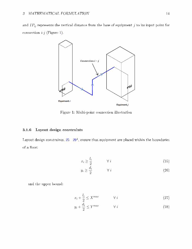
3 MATHEMATICAL FORMULATION 14
and IPij represents the vertical distance from the base of equipment j to its input point for
connection i-j (Figure 1).
Figure 1: Multi-point connection illustration
3.1.6 Layout design constraints
Layout design constraints, 25 - 291, ensure that equipment are placed within the boundaries
of a �oor:
xi ≥li2
∀ i (25)
yi ≥di2
∀ i (26)
and the upper bound:
xi +li2≤ Xmax ∀ i (27)
yi +di2≤ Y max ∀ i (28)

3 MATHEMATICAL FORMULATION 15
The land area is then calculated as:
FA = XmaxY max (29)
An additional layout design constraint is included for the z-coordinates to de�ne its geomet-
rical centre, given by:
zi =hi2
∀ i (30)
Equation 30 also ensures equipment i starts from the base of the �oor k where it is placed.
3.1.7 Area Constraints
In order to avoid bilinear terms in calculating the �oor area, FA (eq. 29), equations 31 - 361
are introduced. The area of each �oor is determined from a set of S prede�ned rectangular
area sizes, ARs, with dimensions (Xs, Y s).
FA =∑s
ARsQs (31)
∑s
Qs = 1 (32)
The �oor length and breadth is selected from the chosen rectangular area size dimensions:
Xmax =∑s
XsQs (33)
Y max =∑s
Y sQs (34)

3 MATHEMATICAL FORMULATION 16
Also, a new term NQs is introduced in order to linearise the cost term associated with the
number of �oors:
NQs ≤ KQs ∀ s (35)
NF =∑s
NQs (36)
3.1.8 Objective function
The objective function is the same for each model - to minimize the total cost associated
with the connection cost, pumping cost, land area cost, �oor construction cost and �oor-area
dependent cost. This is given as:
min∑i
∑j 6=i:fij=1
[CcijTDij + Cv
ijDij + Chij(Rij + Lij + Aij +Bij)]
+FC1 ·NF + FC2∑s
ARs ·NQs + LC · FA(37)
3.2 Formulation B
Formulation B is a linearised model of Ku et al. 18 with adaptations from Patsiatzis and
Papageorgiou 1 as described in the supporting information. The following additional con-
straints are included to account for the multi-�oor equipment and design-speci�ed connection
height.
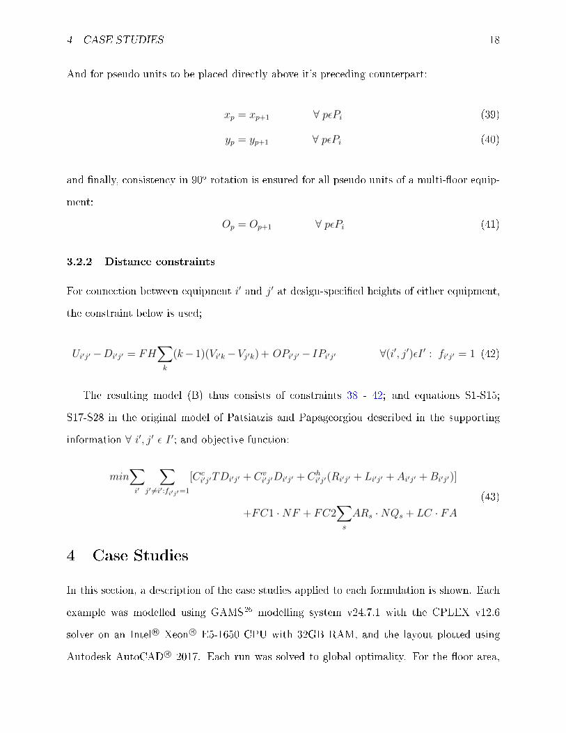
3.2.1 Multi-�oor equipment constraint
Multi-�oor equipment are split into pseudo units equivalent to the number of �oors they
occupy (Figure 2). This approach presents a more accurate representation for multi-�oor
equipment that have varying sizes along its height - due to a range (in type and size) of
auxiliary units placed by such equipment. The drawback, however, is that an increase in
the number of units in the MILP model is realised which can lead to larger computational

3 MATHEMATICAL FORMULATION 17
times.
For all multi-�oor equipment, i ε MF , requiring Mi number of �oors, each is split into Mi
pseudo units. The �rst Mi − 1 units have heights equal to the �oor height, and the last
pseudo unit with the remainder. So, for each i ε MF , there exists pseudo units, p ε Pi; and
the modi�ed set of all equipments, I ′, becomes:
I ′ = (I ∧ (¬MF )) ∨ Pi
Figure 2: Pseudo-unit illustration
Subsequent pseudo units, p + 1, for each pseudo unit set, Pi, are then made to occupy
successive �oors by the constraint:
Vp,k = Vp−1,k−1 ∀ pεPi, k (38)
4 CASE STUDIES 18
And for pseudo units to be placed directly above it's preceding counterpart:
xp = xp+1 ∀ pεPi (39)
yp = yp+1 ∀ pεPi (40)
and �nally, consistency in 90o rotation is ensured for all pseudo units of a multi-�oor equip-
ment:
Op = Op+1 ∀ pεPi (41)
3.2.2 Distance constraints
For connection between equipment i′ and j′ at design-speci�ed heights of either equipment,
the constraint below is used;
Ui′j′ −Di′j′ = FH∑k
(k− 1)(Vi′k−Vj′k)+ OPi′j′ − IPi′j′ ∀(i′, j′)εI ′ : fi′j′ = 1 (42)
The resulting model (B) thus consists of constraints 38 - 42; and equations S1-S15;
S17-S28 in the original model of Patsiatzis and Papageorgiou described in the supporting
information ∀ i′, j′ ε I ′; and objective function:
min∑i′
∑j′ 6=i′:fi′j′=1
[Cci′j′TDi′j′ + Cv
i′j′Di′j′ + Chi′j′(Ri′j′ + Li′j′ + Ai′j′ +Bi′j′)]
+FC1 ·NF + FC2∑s
ARs ·NQs + LC · FA(43)
4 Case Studies
In this section, a description of the case studies applied to each formulation is shown. Each
example was modelled using GAMS26 modelling system v24.7.1 with the CPLEX v12.6
solver on an Intel R© Xeon R© E5-1650 CPU with 32GB RAM, and the layout plotted using
Autodesk AutoCAD R© 2017. Each run was solved to global optimality. For the �oor area,

4 CASE STUDIES 19
�ve alternative sizes (10m, 20m, 30m, 40m and 50m) were used in examples 1 and 2, seven
alternative sizes (10m, 20m, 30m, 40m, 50m, 60m and 70m) in example 3, giving a total
of 25 and 49 possible area sizes respectively, except otherwise stated. Data on connectivity
costs can be obtained from process simulation results of a case study. Pipe sizing values are
obtained from design equations, matched with commercially available pipe sizes and the costs
estimated per unit length for a selected material of construction based on the components in
each stream. Pumping costs are estimated based on current electricity prices and material
�ow rate in each stream, and construction costs are extrapolated from past data on similar
plant design based on structural engineering calculations. For all case studies, data on
equipment dimensions, connectivity and construction costs, and vertical connection points
are included in the supporting information. For all three examples investigated in this work,
both formulations A and B yield equivalent optimal plant layouts and the same objective
value, with main di�erences in layout orientation and re�ection. Thus, only the optimal
layout result for model A.1 is presented for each example. Layout results for the other
models are available in the supporting information.
4.1 Example 1
Example 1 is an Ethylene oxide plant used in the work of Patsiatzis and Papageorgiou 10,
originally presented by Penteado and Ciric 5. The plant consists of 7 units with process
�ow diagram shown in Figure 3. The summary of the model statistics and computational
performance is shown in Table 2 and the optimal layout in Figure 4.
The results obtained gave a total cost of 66,262.0 rmu - 22% connection costs, 44%
pumping costs and 34% construction costs. Each �oor had an area measuring 20mx20m,
totalling two �oors selected for construction out of four provided to the model. Table 2
shows that the models in formulation A are more computationally e�cient. Formulation B
was inherently larger in size for each case study, as a greater number of units needed to be
handled than in formulations A.

4 CASE STUDIES 20
Figure 3: Flow diagram of Ethylene Oxide plant
The layout of equipment in Figure 4 showed that the two multi-�oor equipment (3 and
5) started on the �rst �oor and terminated on the second �oor for all models, as they
require two �oors based on their height. The total cost - 66,262.0 rmu - is also greater
than the value obtained by Patsiatzis and Papageorgiou 1 (50,817 rmu). The 30% increase
in cost is attributed to the additional consideration of the connection points being measured
from the design-speci�ed heights, and the consequent change in equipment layout. Previous
considerations assumed a connection from the mid-point of an equipment height, but current
results show that such assumption is not realistic as re�ected in the cost di�erence.
Table 2: Summary of model statistics and computational performance for Example 1
EO plant (7 units)A.1 A.2 A.3 B
Total Cost (rmu) 66,262.0CPU (s) 1.5 1.4 1.7 3.0Number of binary variables 112 112 112 167Number of continuous variables 225 204 225 130Number of equations 424 381 382 633

4 CASE STUDIES 21
Figure 4: Example 1 layout results
4.2 Example 2
Example 2 is an Urea production plant, simulated with Aspen PLUS R© v8.0. It consists of
8 units, 2 of which exceed the �oor height of 8m. The process �ow diagram of the plant is
shown in Figure 5. A total of 25 possible area sizes were used ranging from 5m - 45m. Each
unit had to be placed a minimum of 4m from another in either direction. The summary of
the model statistics and computational performance is shown in Table 3.
The layout result is shown in Figure 6. All 4 �oors were assigned units, with each �oor
having an area measuring 15mx5m, and a total cost of 117,431.0 rmu - 6% connection, 26%
pumping and 68% construction costs. The two multi-�oor units (units 2 and 4) occupied
successive �oors proportional to their height (�oors 1-4 and 2-3 respectively). Computational
results showed global optimality was achieved by all models in a relatively short time (under
5s). Overall results show that the model is capable of handling process-speci�c conditions
whilst deciding �oor placement even for multi-�oor units.

4 CASE STUDIES 22
Figure 5: Flow diagram of Urea Production
Table 3: Summary of model statistics and computational performance for Example 2
Urea Production (8 units)A.1 A.2 A.3 B
Total Cost (rmu) 117,431.0CPU (s) 4.8 4.9 2.9 4.0Number of binary variables 145 145 1453 281Number of continuous variables 315 283 315 159Number of equations 611 547 547 1,279

4 CASE STUDIES 23
Figure 6: Example 2 layout results

4 CASE STUDIES 24
4.3 Example 3
Example 3 is a Crude Distillation plant with preheating train, simulated with Aspen HYSYS R©
v8.0. It consists of 17 units, with 5 (pre-�ash drum (unit 5), atmospheric distillation tower
(unit 7), �red heaters 1 and 2 (unit 6 and 12), and debutaniser(unit 15)) exceeding the �oor
height of 5m. The process �ow diagram of the plant is shown in Figure 7.
An additional condition that each of the multi-�oor equipment starts from the ground �oor
Figure 7: Flow diagram of Crude Distillation Plant with Preheating train
was imposed, as such represents a realistic representation from a construction point of view.
The summary of the model statistics and computational performance is shown in Table 4
and the optimal layout in Figure 8.
The results obtained gave a total of four(4) possible �oors, out of an available seven (7)
which each �oor measuring 20mx20m. A total cost of 749,691.4 rmu was obtained across all
formulations as seen in Table 4. The higher relative pumping costs (50%) when compared

4 CASE STUDIES 25
with previous examples is attributed to the greater number of units considered. Connection
and construction costs constituted 6% and 44% of the total cost respectively.
Table 4: Summary of model statistics and computational performance for Example 3
CDU Plant (17 units)A.1 A.2 A.3 B
Total Cost (rmu) 749,691.4CPU (s) 292.3 105.0 44.1 131.6Number of binary variables 568 568 568 1,569Number of continuous variables 1,507 1,388 1,507 387Number of equations 3,213 2,993 2,975 11,483
The layout of equipment is shown in Figure 8. As all the multi-�oor equipment (5, 6,
7, 12 and 15) starting �oors were prede�ned, they all started from the �rst �oor through
the number of �oors required based on their height. It is worthy of noting that although
equipment 14 required 5 �oors based on its height, a total of 4 �oors was decided by all
formulations. This is because the construction of a �fth �oor was deemed unnecessary as no
other equipment other than equipment 14 was to be placed on such �oor in order to obtain
an optimal solution, and the additional construction cost for a �fth �oor was eliminated. So,
although a multi-�oor equipment can span a speci�ed number of �oors based on its height,
not every one of those �oors need to be constructed. Practical examples include multi-�oor
layouts about �red heaters with long stacks, distillation columns and �are stacks.
Figure 8: Example 3 layout results

4 CASE STUDIES 26
4.3.1 Symmetry breaking constraints
For each of the case studies solved, it becomes evident from the layout results (presented
above and in supporting information) that there can exist multiple optimal solutions for
each problem. These multiple optimal solutions di�er only in layout orientation/re�ection
and/or translation of equipment on the layout area, resulting in ine�cient CPU usage27,
especially for larger problem instances. In order to increase computational e�ciency and
reduce symmetry, additional constraints, adapted from Westerlund and Papageorgiou 27 are
introduced:
xi + yi − xj − yj ≥ α ·Nij (44)
E1ij = 0 (45)
where α = min(li2, di
2
)+min
(lj2,dj2
). These �x the relative position of i and j as well as one
of the non-overlapping binary variables, E1ij = 0. The latter enforces either of xi−xj ≥ li+lj2
or yi− yj ≥ di+dj2
according to equations 17 - 20, i.e., unit i is relatively locked in a compass
point North East of unit j hence breaking the symmetry.
The above symmetry breaking constraints were applied to example 3 - Crude distillation
plant with pre-heating train - by incorporating equations 44 and 45 in Model A.1 where the
choice of equipment i and j are among multi-�oor units only, based on the following three
criteria27:
a - Equipment i and j having the highest connection cost: units 5 and 6;
b - Two equipment with the largest area: units 7 and 15;
c - Two equipment with the smallest area: units 6 and 12.
The resulting models were solved to global optimality and a solution of 749,691.4 rmu was
obtained in all alternative choices of equipment, the same as model A.1 without these con-
straints. Their computational CPU times are shown in Table 5 - where for each unit selection

5 CONCLUDING REMARKS 27
alternative, the resulting model is named appropriately - model A.1a for model A.1 with sym-
metry breaking constraints with equipment i and j chosen by criterion a, having the highest
connection cost, and so on. The results show that the new symmetry breaking constraints has
improved computational e�ciency by one order of magnitude. Computational improvements
were also found for the other models developed and examples presented in this work.
Table 5: Summary of computational performance for Example 3; Model A.1 with symmetrybreaking contraints
Model CPU (s)A.1 292.3A.1a 31.2A.1b 33.7A.1c 71.2
5 Concluding remarks
An extension of the MILP model by Patsiatzis and Papageorgiou 1 was proposed to address
new concerns in the multi-�oor process plant layout problem. These concerns included the
presence of multi-�oor equipment in certain process plants with design-speci�ed input and
output connection points along the height of an equipment.
A total of four (4) models were proposed, grouped in two broad classes. The �rst class
handled multi-�oor equipment as they were (single tall units) having constraints to ensure
multi-�oor equipment were assigned to consecutive �oors, with three (3) alternative models
resulting. For the second class, multi-�oor equipment were broken up to single-�oor-pseudo-
units and the layout solved based on a linearised model of Ku et al. 18.
Each of the four (4) models were validated with case studies and model performance were
ascertained and compared. All models solved problems of up to 17 units well under 7 minutes,
as compared to previous work1 which only handled a maximum of 11 units simultaneously.
Total cost distribution were consistent with expected values - construction and pumping
costs taken up the larger portion, with connection costs following. All models were able to

5 ACKNOWLEDGEMENT 28
handle multi-�oor equipment, and decide whether a �oor be constructed and used even if a
multi-�oor equipment were assigned to it. In most cases though, formulations A was found
to be more computationally e�cient than B.
Finally, symmetry breaking constraints were introduced reducing the availability of multiple
optimal solutions that lead to greater CPU usage. These constraints �xed the relative
positions of two units i and j. The choice of units i and j were based on three criteria: largest
connection, largest areas or smallest area amongst multi-�oor equipment. A reduction in
computational time up to 31.2s was obtained for example 3, as compared to 292.3s without
symmetry breaking.
Further work will entail model validation with larger case studies and the development of
e�cient computational methods, e.g. decomposition techniques.
Acknowledgement
JOE acknowledges the �nancial support of the Petroleum Technology Development Fund
(PTDF), Nigeria.
Supporting Information Available
A full description of the model proposed by Patsiatzis and Papageorgiou 1, data for the case
studies presented, and layout results for models A.2, A.3 and B is available as supporting
information.
Author Information
Corresponding Author
*Email: [email protected]; Phone: +44 (0)20 7679 2563.

5 AUTHOR INFORMATION 29
ORCID
Songsong Liu: 0000-0001-8412-274X
Lazaros G. Papageorgiou: 0000-0003-4652-6086
Notes
The authors declare no competing �nancial interest.

5 REFERENCES 30
References
(1) Patsiatzis, D. I.; Papageorgiou, L. G. E�cient Solution Approaches for the Multi�oor
Process Plant Layout Problem. Industrial & Engineering Chemistry Research 2003,
42, 811�824.
(2) Anjos, M. F.; Vieira, M. V. C. Mathematical Optimization Approaches for Facility Lay-
out Problems: The State-of-the-Art and Future Research Directions. European Journal
of Operational Research 2017, 261, 1�16.
(3) Mecklenburgh, J. Process plant layout, 2nd ed.; Longman: New York, 1985; p 625.
(4) Drira, A.; Pierreval, H.; Hajri-Gabouj, S. Facility layout problems: A survey. Annual
Reviews in Control 2007, 31, 255�267.
(5) Penteado, F. D.; Ciric, A. R. An MINLP Approach for Safe Process Plant Layout.
Industrial & Engineering Chemistry Research 1996, 35, 1354�1361.
(6) Guirardello, R.; Swaney, R. E. Optimization of process plant layout with pipe routing.
Computers & Chemical Engineering 2005, 30, 99�114.
(7) Barbosa-Povoa, A. P.; Mateusz, R.; Novaisz, A. Q. Optimal two-dimensional layout of
industrial facilities. International Journal of Production Research 2001, 3912, 2567�
2593.
(8) Barbosa-Póvoa, A. P.; Mateus, R.; Novais, A. Q. Optimal 3D layout of industrial
facilities. International Journal of Production Research 2002, 40, 1669�1698.
(9) Georgiadis, M.; Macchietto, S. Layout of process plants: A novel approach. Computers
& Chemical Engineering 1997, 21, S337�S342.
(10) Patsiatzis, D. I.; Papageorgiou, L. G. Optimal multi-�oor process plant layout. Com-
puters & Chemical Engineering 2002, 26, 575�583.

5 REFERENCES 31
(11) Patsiatzis, D. I.; Knight, G.; Papageorgiou, L. G. An MILP approach to safe process
plant layout. Chemical Engineering Research and Design 2004, 82, 579�586.
(12) Papageorgiou, L. G.; Rotstein, G. E. Continuous-domain mathematical models for op-
timal process plant layout. Industrial & Engineering Chemistry Research 1998, 5885,
3631�3639.
(13) Xu, G.; Papageorgiou, L. G. Process plant layout using an improvement-type algorithm.
Chemical Engineering Research and Design 2009, 87, 780�788.
(14) Medina-Herrera, N.; Jiménez-Gutiérrez, A.; Grossmann, I. E. A mathematical program-
ming model for optimal layout considering quantitative risk analysis. Computers and
Chemical Engineering 2014, 68, 165�181.
(15) Huang, C.; Wong, C. K. Optimisation of site layout planning for multiple construction
stages with safety considerations and requirements. Automation in Construction 2015,
53, 58�68.
(16) Jung, S. Facility siting and plant layout optimization for chemical process safety.Korean
Journal of Chemical Engineering 2016, 33, 1�7.
(17) Xin, P.; Khan, F.; Ahmed, S. Layout Optimization of a Floating Lique�ed Natural Gas
Facility Using Inherent Safety Principles. Journal of O�shore Mechanics and Arctic
Engineering 2016, 138, 041602.
(18) Ku, N.-K.; Hwang, J.-H.; Lee, J.-C.; Roh, M.-I.; Lee, K.-Y. Optimal module layout for a
generic o�shore LNG liquefaction process of LNG-FPSO. Ships and O�shore Structures
2013, 9, 311�332.
(19) Hwang, J.; Lee, K. Y. Optimal liquefaction process cycle considering simplicity and
e�ciency for LNG FPSO at FEED stage. Computers and Chemical Engineering 2014,
63, 1�33.

5 REFERENCES 32
(20) Ku, N.; Jeong, S.-Y.; Roh, M.-I.; Shin, H.-K.; Ha, S.; Hong, J.-w. Layout Method of a
FPSO (Floating, Production, Storage, and O�-Loading Unit) Using the Optimization
Technique. Volume 1B: O�shore Technology. 2014; pp 1�11.
(21) Park, P. J.; Lee, C. J. The Research of Optimal Plant Layout Optimization based on
Particle Swarm Optimization for Ethylene Oxide Plant. Journal of the Korean Society
of Safety 2015, 30, 32�37.
(22) Kheirkhah, A.; Navidi, H.; Messi Bidgoli, M. Dynamic facility layout problem: a new
bilevel formulation and some metaheuristic solution methods. IEEE Transactions on
Engineering Management 2015, 62, 396�410.
(23) Navidi, H.; Bashiri, M.; Bidgoli, M. M. A heuristic approach on the facility layout
problem based on game theory. International Journal of Production Research 2012,
50, 1512�1527.
(24) Nabavi, S. R.; Taghipour, A. H.; Mohammadpour Gorji, A. Optimization of Facility
Layout of Tank farms using Genetic Algorithm and Fireball Scenario. Chemical Product
and Process Modeling 2016, 11 .
(25) Furuholmen, M.; Glette, K.; Hovin, M.; Torresen, J. A coevolutionary, hyper heuristic
approach to the optimization of three-dimensional process plant layouts - A comparative
study. 2010 IEEE World Congress on Computational Intelligence, WCCI 2010 - 2010
IEEE Congress on Evolutionary Computation, CEC 2010 2010,
(26) Rosenthal, E. GAMS-A user's guide. GAMS Development Corporation. Washington,
DC, USA, 2008.
(27) Westerlund, J.; Papageorgiou, L. G. Improved Performance in Process Plant Layout
Problems Using Symmetry-breaking constraints. Design 2002, 485�488.

5 REFERENCES 33
Graphical TOC Entry